Estimating ice phenology on large northern lakes - The Cryosphere

The Cryosphere, 6, 235–254, 2012www.the-cryosphere.net/6/235/2012/doi:10.5194/tc-6-235-2012© Author(s) 2012. CC Attribution 3.0 License.

The Cryosphere

Estimating ice phenology on large northern lakes from AMSR-E:algorithm development and application to Great Bear Lake andGreat Slave Lake, Canada

K.-K. Kang 1,2, C. R. Duguay1,2, and S. E. L. Howell3

1Interdisciplinary Centre on Climate Change (IC3), University of Waterloo, Waterloo, Ontario N2L 3G1, Canada2Department of Geography and Environmental Management, University of Waterloo, Waterloo, Ontario N2L 3G1, Canada3Climate Research Division, Environment Canada, 4905 Dufferin Street, Toronto, Ontario M3H 5T4, Canada

Correspondence to:K.-K. Kang ([email protected])

Received: 9 October 2011 – Published in The Cryosphere Discuss.: 14 November 2011Revised: 4 February 2012 – Accepted: 23 February 2012 – Published: 8 March 2012

Abstract. Time series of brightness temperatures (TB) fromthe Advanced Microwave Scanning Radiometer–Earth Ob-serving System (AMSR-E) are examined to determine icephenology variables on the two largest lakes of northernCanada: Great Bear Lake (GBL) and Great Slave Lake(GSL). TB measurements from the 18.7, 23.8, 36.5, and89.0 GHz channels (H- and V- polarization) are comparedto assess their potential for detecting freeze-onset/melt-onsetand ice-on/ice-off dates on both lakes. The 18.7 GHz (H-pol) channel is found to be the most suitable for estimatingthese ice dates as well as the duration of the ice cover and ice-free seasons. A new algorithm is proposed using this channeland applied to map all ice phenology variables on GBL andGSL over seven ice seasons (2002–2009). Analysis of thespatio-temporal patterns of each variable at the pixel levelreveals that: (1) both freeze-onset and ice-on dates occur onaverage about one week earlier on GBL than on GSL (Dayof Year (DY) 318 and 333 for GBL; DY 328 and 343 forGSL); (2) the freeze-up process or freeze duration (freeze-onset to ice-on) takes a slightly longer amount of time onGBL than on GSL (about 1 week on average); (3) melt-onsetand ice-off dates occur on average one week and approxi-mately four weeks later, respectively, on GBL (DY 143 and183 for GBL; DY 135 and 157 for GSL); (4) the break-upprocess or melt duration (melt-onset to ice-off) lasts on aver-age about three weeks longer on GBL; and (5) ice cover dura-tion estimated from each individual pixel is on average aboutthree weeks longer on GBL compared to its more southerncounterpart, GSL. A comparison of dates for several ice phe-nology variables derived from other satellite remote sensingproducts (e.g. NOAA Interactive Multisensor Snow and Ice

Mapping System (IMS), QuikSCAT, and Canadian Ice Ser-vice Database) show that, despite its relatively coarse spatialresolution, AMSR-E 18.7 GHz provides a viable means formonitoring of ice phenology on large northern lakes.

1 Introduction

Lake ice cover is an important component of the terrestrialcryosphere for several months of the year in high-latituderegions (Duguay et al., 2003). Lake ice is not only a sen-sitive indicator of climate variability and change, but it alsoplays a significant role in energy and water balance at lo-cal and regional scales. The presence of an ice cover alterslake-atmosphere exchanges (Duguay et al., 2006; Brown andDuguay, 2010). When energy movement occurs during tem-perature change, heat transfer (thermodynamics) influencesice thickening as well as the timing and duration of freeze-upand break-up processes, which is referred to as ice phenology(Jeffries and Morris, 2007). Lake ice phenology, which en-compasses freeze-onset/melt-onset, ice-on/ice-off dates, andice cover duration, is largely influenced by air temperaturechanges and is therefore a robust indicator of climate condi-tions (e.g. Bonsal et al., 2006; Duguay et al., 2006; Kouraevet al., 2007; Latifovic and Pouliot, 2007; Schertzer et al.,2008; Howell et al., 2009).

The analysis of historical trends (1846–1995) in in situ ob-servations of lake and river ice phenology has provided ev-idence of later freeze–up (ice-on) and earlier break-up (ice-off) dates at the northern hemispheric scale (Magnuson et al.,2000; Brown and Duguay, 2010). In Canada, from 1951 to

Published by Copernicus Publications on behalf of the European Geosciences Union.

236 K.-K. Kang et al.: Estimating ice phenology on large northern lakes from AMSR-E

2000, trends towards earlier ice-off dates have been observedfor many lakes, but ice-on dates have shown few significanttrends over the same period (Duguay et al., 2006). The ob-served changes in Canada’s lake ice cover have also beenfound to be influenced by large-scale atmospheric forcings(Bonsal et al., 2006). Canada’s government-funded histori-cal ground-based observational network has provided muchof the evidence for the documented changes for most of the20th century and for establishing links with variations in at-mospheric teleconnection indices, notably Pacific oscillationpatterns such as Pacific North American Pattern and PacificDecadal Oscillation. Unfortunately, the Canadian ground-based lake ice network has been eroded to the point where itcan no longer provide the quantity of observations necessaryfor climate monitoring across the country. Satellite remotesensing is the most logical means for establishing a globalobservational network as the reduction in the ground-basedlake ice network seen in Canada has been mimicked in manyother countries of the Northern Hemisphere (IGOS, 2007).

From a satellite remote sensing perspective, dates asso-ciated with estimating the freeze-up process (i.e. onset offreeze until a complete sheet of ice is formed) in autumnand early winter are particularly difficult to determine us-ing optical satellite sensors such as the Moderate Resolu-tion Imaging Spectroradiometer (MODIS) and the AdvancedVery High Resolution Radiometer (AVHRR) on high-latitudelakes due to long periods of obscuration by darkness and ex-tensive cloud cover (Maslanik et al., 1987; Jeffries et al.,2005; Latifovic and Pouliot, 2007). QuikSCAT has beenused successfully to derive and map freeze-onset, melt-onsetand ice-off dates on Great Bear Lake (GBL) and Great SlaveLake (GSL) (Howell et al., 2009). Unfortunately, QuikSCATdata are no longer available for lake ice monitoring on largelakes since its nominal mission ended on 23 November 2009.Previous investigations have shown the utility of observ-ing lake ice phenology variables through the visual inter-pretation of brightness temperature (TB) changes from theScanning Multichannel Microwave Radiometer (SMMR) at37 GHz (Barry and Maslanik, 1993) and the Special SensorMicrowave/Imager (SSM/I) at 85 GHz (Walker et al., 1993,2000) on GSL, but identifying spatial variability in thesevariables is difficult due to their coarse resolution (∼25 km).In a recent study, SSM/I has been used in combination withradar altimetry to determine automatically ice phenologyevents on Lake Baikal (Kouraev et al., 2007).

Measurements by the Advanced Microwave ScanningRadiometer–Earth Observing System (AMSR-E) that offerimproved spatial resolution have yet to be assessed for mon-itoring ice phenology. The objectives of this paper are to(i) evaluate the utility of AMSR-ETB measurements for es-timating lake ice phenology, (ii) develop a comprehensivealgorithm for mapping lake ice phenology variables, and(iii) apply the algorithm over both GBL and GSL to investi-gate the spatio-temporal variability of each lakes ice phonol-ogy from 2002 to 2009.

2 Background

2.1 Passive microwave radiometry of lake ice

The discrimination of ice cover characteristics from passivemicrowave brightness temperature (TB) measurements re-quires a good knowledge of the radiometric properties of icein nature (Kouraev et al., 2007). In contrast to the high-loss characteristics of sea ice (due to salinity), one of themajor microwave characteristics of pure freshwater ice is itslow-loss transmission behavior (Ulaby et al., 1986). TheTBat passive microwave frequencies is defined as the productof the emissivity (ε) and physical temperature (Tkin) of themedium:

TB = εTkin (1)

Passive microwave systems can measure, regardless of cloudcoverage and darkness, naturally emitted radiation throughTB. Since emissivity ranges between 0 and 1, theTB islower than the kinetic temperature of the medium. Thelarge change in emissivity from open water (ε = 0.443–0.504 at 24 GHz) to ice covered conditions (ε = 0.858–0.908at 24 GHz) (Hewison and English, 1999; Hewison, 2001)makes the determination of the timing of ice formation anddecay on large, deep lakes, feasible fromTB measurements.The emissivity of ice, and thereforeTB, further increasesfrom its initial formation as the effect of the radiometricallycold water under the ice cover decreases with ice thickening(Kang et al., 2010).

2.2 Definitions of ice phenology variables

The definitions of freeze-up and break-up are opposite: theformer describes the time period between the beginning ofice formation and the formation of a complete sheet of ice,while the latter describes the time period between the onsetof spring melt and the complete disappearance of ice fromthe lake surface. Since the algorithm presented herein oper-ates on a pixel-by-pixel basis and is applied over entire lakesurfaces, it is important to provide clear definitions of the icephenology variables as they relate to individual pixels andover whole lakes (or lake sections) (Table 1). At the levelof the pixel, the freeze-up period encompasses freeze onset(FO), ice-on and freeze duration (FD), while the break-upperiod comprises melt onset (MO), ice off and melt duration(MD). The period between ice-on and ice-off covers an iceseason and is referred to as ice cover duration (ICDp; p forpixel). At the lake or lake section level (third column of Ta-ble 1), complete freeze over (CFO), water clear of ice (WCI)and ice cover duration (ICDe; e for entire lake or lake sec-tions as to avoid land contamination in some AMSR-ETBmeasurements) are the terms used from here onward. CFOcorresponds to the date when all pixels within the lake or lakesection have become ice-covered (i.e. all flagged with havingice-on). WCI corresponds to the date when all pixels have

The Cryosphere, 6, 235–254, 2012 www.the-cryosphere.net/6/235/2012/

K.-K. Kang et al.: Estimating ice phenology on large northern lakes from AMSR-E 237

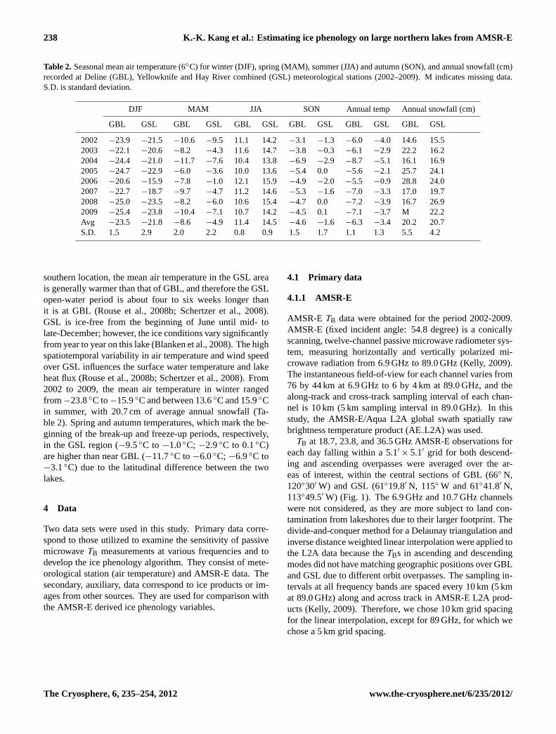
Table 1. Definition of ice phenology variables at per pixel level and for entire lake or lake section.

Pixel level Entire lake or lake section

Freeze-upPeriod

Freeze onset (FO): First day of the year on which thepresence of ice is detected in a pixel and remains untilice-onIce-on: Day of the year on which a pixel becomestotally ice-coveredFreeze duration (FD): number of days betweenfreeze-onset and ice-on dates

Complete freeze over (CFO):Day of the year when all pixels become totally ice-covered

Break-upperiod

Melt onset (MO): First day of the year on which gen-eralized spring melt begins in a pixelIce-off: Day of the year on which a pixel becomestotally ice-freeMelt duration (MD): numbers of days between melt-onset and ice-off dates

Water clear of ice (WCI):Day of the year when all pixels become totally ice-free

Ice season Ice cover duration (ICDp): number of days betweenice-on and ice-off dates

Ice cover duration (ICDe): number of days betweenCFO and WCI

become ice-free (i.e. all flagged with having ice-off). WhileICDp is calculated for each individual pixel from dates ofice-on to ice-off, ICDe is determined as the number of daysbetween CFO and WCI within an ice season.

3 Study area

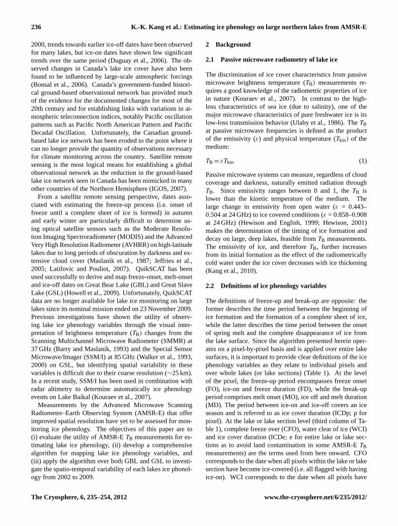
GBL and GSL are two of the largest freshwater lakes in theworld. Located in the Mackenzie River Basin they fall withintwo physiographic regions of Canada’s Northwest Territo-ries: the Precambrian Shield and the Interior Plains (Fig. 1).The eastern parts of both lakes are situated in the Precam-brian Shield. Its undulating topography with bedrock out-crops causes the formation of rounded hills and valleys. Thehigh topography of the western Cordillera and low relief ofthe central and eastern parts of the Mackenzie Basin stronglyinfluence the regional climate (e.g. atmospheric circulationpattern and the advective heat and moisture fluxes) (Woo etal., 2008). Most of GBL and the western/central parts of GSLare located in the flat-lying Interior Plains and underlain bythick glacial, fluvial, and lacustrine deposits; in addition, thePlains are dotted with numerous wetlands and lakes (Wooet al., 2008). GBL and GSL lie between 60◦ to 67◦ N andbetween 109◦ to 126◦ W (Fig. 1), and, respectively, have sur-face areas of 31.3× 103 km2 and 28.6× 103 km2, and aver-age depths of 76 m and 88 m (Rouse et al., 2008a; Woo et al.,2008). The northern extent of GBL is influenced by coldertemperatures than its more southern counterpart (Rouse etal., 2008b).

From 2002 to 2009, the period of analysis of this study, theaverage air temperature recorded at the Deline weather sta-tion (65◦12′ N, 123◦26′ W), near the western shore of GBL,ranged between−25.4◦C and−20.6◦C for winter (DJF) and

Fig. 1. Map showing location of Great Bear Lake (GBL) and GreatSlave Lake (GSL), and their meteorological stations (Deline, Yel-lowknife, and Hay River) within the Mackenzie River Basin. Solidsquares represent 5.1′

× 5.1′ (9.48 km× 9.48 km) of sampling sitesat 18.7 GHz for the development of the ice phenology algorithm.Arrows indicate river flow direction.

from 10.0◦C to 12.1◦C for summer (JJA) with 20.2 cm ofaverage annual snowfall (Table 2). For GBL, complete wa-ter turnover occurs at least in some parts of the lake and nobreak-up occurs until early July (Rouse et al., 2008a).

GSL is part of the north-flowing river system in theMackenzie Basin (Rouse et al., 2008b). Situated at a more

www.the-cryosphere.net/6/235/2012/ The Cryosphere, 6, 235–254, 2012


Table 2. Seasonal mean air temperature (6◦C) for winter (DJF), spring (MAM), summer (JJA) and autumn (SON), and annual snowfall (cm)recorded at Deline (GBL), Yellowknife and Hay River combined (GSL) meteorological stations (2002–2009). M indicates missing data.S.D. is standard deviation.

DJF MAM JJA SON Annual temp Annual snowfall (cm)

GBL GSL GBL GSL GBL GSL GBL GSL GBL GSL GBL GSL

2002 −23.9 −21.5 −10.6 −9.5 11.1 14.2 −3.1 −1.3 −6.0 −4.0 14.6 15.52003 −22.1 −20.6 −8.2 −4.3 11.6 14.7 −3.8 −0.3 −6.1 −2.9 22.2 16.22004 −24.4 −21.0 −11.7 −7.6 10.4 13.8 −6.9 −2.9 −8.7 −5.1 16.1 16.92005 −24.7 −22.9 −6.0 −3.6 10.0 13.6 −5.4 0.0 −5.6 −2.1 25.7 24.12006 −20.6 −15.9 −7.8 −1.0 12.1 15.9 −4.9 −2.0 −5.5 −0.9 28.8 24.02007 −22.7 −18.7 −9.7 −4.7 11.2 14.6 −5.3 −1.6 −7.0 −3.3 17.0 19.72008 −25.0 −23.5 −8.2 −6.0 10.6 15.4 −4.7 0.0 −7.2 −3.9 16.7 26.92009 −25.4 −23.8 −10.4 −7.1 10.7 14.2 −4.5 0.1 −7.1 −3.7 M 22.2Avg −23.5 −21.8 −8.6 −4.9 11.4 14.5 −4.6 −1.6 −6.3 −3.4 20.2 20.7S.D. 1.5 2.9 2.0 2.2 0.8 0.9 1.5 1.7 1.1 1.3 5.5 4.2

southern location, the mean air temperature in the GSL areais generally warmer than that of GBL, and therefore the GSLopen-water period is about four to six weeks longer thanit is at GBL (Rouse et al., 2008b; Schertzer et al., 2008).GSL is ice-free from the beginning of June until mid- tolate-December; however, the ice conditions vary significantlyfrom year to year on this lake (Blanken et al., 2008). The highspatiotemporal variability in air temperature and wind speedover GSL influences the surface water temperature and lakeheat flux (Rouse et al., 2008b; Schertzer et al., 2008). From2002 to 2009, the mean air temperature in winter rangedfrom−23.8◦C to−15.9◦C and between 13.6◦C and 15.9◦Cin summer, with 20.7 cm of average annual snowfall (Ta-ble 2). Spring and autumn temperatures, which mark the be-ginning of the break-up and freeze-up periods, respectively,in the GSL region (−9.5◦C to −1.0◦C; −2.9◦C to 0.1◦C)are higher than near GBL (−11.7◦C to −6.0◦C; −6.9◦C to−3.1◦C) due to the latitudinal difference between the twolakes.

4 Data

Two data sets were used in this study. Primary data corre-spond to those utilized to examine the sensitivity of passivemicrowaveTB measurements at various frequencies and todevelop the ice phenology algorithm. They consist of mete-orological station (air temperature) and AMSR-E data. Thesecondary, auxiliary, data correspond to ice products or im-ages from other sources. They are used for comparison withthe AMSR-E derived ice phenology variables.

4.1 Primary data

4.1.1 AMSR-E

AMSR-E TB data were obtained for the period 2002-2009.AMSR-E (fixed incident angle: 54.8 degree) is a conicallyscanning, twelve-channel passive microwave radiometer sys-tem, measuring horizontally and vertically polarized mi-crowave radiation from 6.9 GHz to 89.0 GHz (Kelly, 2009).The instantaneous field-of-view for each channel varies from76 by 44 km at 6.9 GHz to 6 by 4 km at 89.0 GHz, and thealong-track and cross-track sampling interval of each chan-nel is 10 km (5 km sampling interval in 89.0 GHz). In thisstudy, the AMSR-E/Aqua L2A global swath spatially rawbrightness temperature product (AEL2A) was used.

TB at 18.7, 23.8, and 36.5 GHz AMSR-E observations foreach day falling within a 5.1′ × 5.1′ grid for both descend-ing and ascending overpasses were averaged over the ar-eas of interest, within the central sections of GBL (66◦ N,120◦30′ W) and GSL (61◦19.8′ N, 115◦ W and 61◦41.8′ N,113◦49.5′ W) (Fig. 1). The 6.9 GHz and 10.7 GHz channelswere not considered, as they are more subject to land con-tamination from lakeshores due to their larger footprint. Thedivide-and-conquer method for a Delaunay triangulation andinverse distance weighted linear interpolation were applied tothe L2A data because theTBs in ascending and descendingmodes did not have matching geographic positions over GBLand GSL due to different orbit overpasses. The sampling in-tervals at all frequency bands are spaced every 10 km (5 kmat 89.0 GHz) along and across track in AMSR-E L2A prod-ucts (Kelly, 2009). Therefore, we chose 10 km grid spacingfor the linear interpolation, except for 89 GHz, for which wechose a 5 km grid spacing.



4.1.2 Meteorological station data

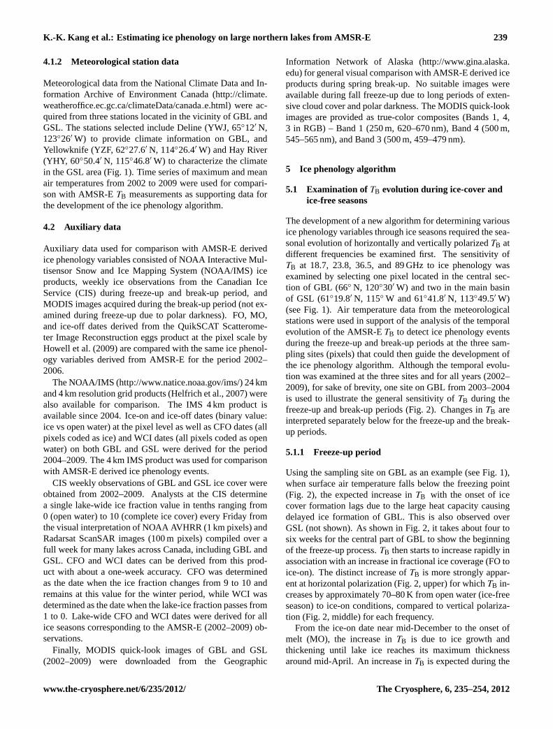
Meteorological data from the National Climate Data and In-formation Archive of Environment Canada (http://climate.weatheroffice.ec.gc.ca/climateData/canadae.html) were ac-quired from three stations located in the vicinity of GBL andGSL. The stations selected include Deline (YWJ, 65◦12′ N,123◦26′ W) to provide climate information on GBL, andYellowknife (YZF, 62◦27.6′ N, 114◦26.4′ W) and Hay River(YHY, 60◦50.4′ N, 115◦46.8′ W) to characterize the climatein the GSL area (Fig. 1). Time series of maximum and meanair temperatures from 2002 to 2009 were used for compari-son with AMSR-ETB measurements as supporting data forthe development of the ice phenology algorithm.

4.2 Auxiliary data

Auxiliary data used for comparison with AMSR-E derivedice phenology variables consisted of NOAA Interactive Mul-tisensor Snow and Ice Mapping System (NOAA/IMS) iceproducts, weekly ice observations from the Canadian IceService (CIS) during freeze-up and break-up period, andMODIS images acquired during the break-up period (not ex-amined during freeze-up due to polar darkness). FO, MO,and ice-off dates derived from the QuikSCAT Scatterome-ter Image Reconstruction eggs product at the pixel scale byHowell et al. (2009) are compared with the same ice phenol-ogy variables derived from AMSR-E for the period 2002–2006.

The NOAA/IMS (http://www.natice.noaa.gov/ims/) 24 kmand 4 km resolution grid products (Helfrich et al., 2007) werealso available for comparison. The IMS 4 km product isavailable since 2004. Ice-on and ice-off dates (binary value:ice vs open water) at the pixel level as well as CFO dates (allpixels coded as ice) and WCI dates (all pixels coded as openwater) on both GBL and GSL were derived for the period2004–2009. The 4 km IMS product was used for comparisonwith AMSR-E derived ice phenology events.

CIS weekly observations of GBL and GSL ice cover wereobtained from 2002–2009. Analysts at the CIS determinea single lake-wide ice fraction value in tenths ranging from0 (open water) to 10 (complete ice cover) every Friday fromthe visual interpretation of NOAA AVHRR (1 km pixels) andRadarsat ScanSAR images (100 m pixels) compiled over afull week for many lakes across Canada, including GBL andGSL. CFO and WCI dates can be derived from this prod-uct with about a one-week accuracy. CFO was determinedas the date when the ice fraction changes from 9 to 10 andremains at this value for the winter period, while WCI wasdetermined as the date when the lake-ice fraction passes from1 to 0. Lake-wide CFO and WCI dates were derived for allice seasons corresponding to the AMSR-E (2002–2009) ob-servations.

Finally, MODIS quick-look images of GBL and GSL(2002–2009) were downloaded from the Geographic

Information Network of Alaska (http://www.gina.alaska.edu) for general visual comparison with AMSR-E derived iceproducts during spring break-up. No suitable images wereavailable during fall freeze-up due to long periods of exten-sive cloud cover and polar darkness. The MODIS quick-lookimages are provided as true-color composites (Bands 1, 4,3 in RGB) – Band 1 (250 m, 620–670 nm), Band 4 (500 m,545–565 nm), and Band 3 (500 m, 459–479 nm).

5 Ice phenology algorithm

5.1 Examination ofTB evolution during ice-cover andice-free seasons

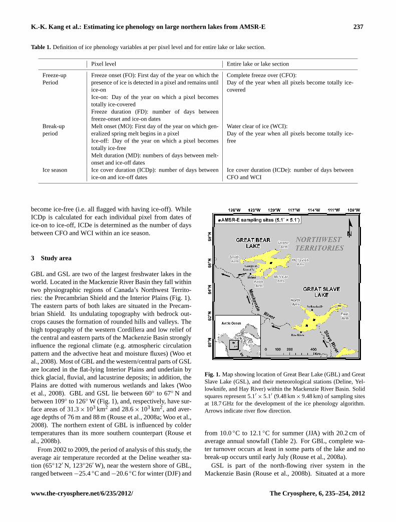
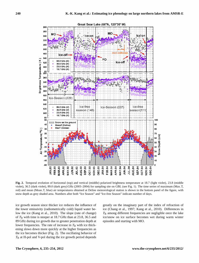
The development of a new algorithm for determining variousice phenology variables through ice seasons required the sea-sonal evolution of horizontally and vertically polarizedTB atdifferent frequencies be examined first. The sensitivity ofTB at 18.7, 23.8, 36.5, and 89 GHz to ice phenology wasexamined by selecting one pixel located in the central sec-tion of GBL (66◦ N, 120◦30′ W) and two in the main basinof GSL (61◦19.8′ N, 115◦ W and 61◦41.8′ N, 113◦49.5′ W)(see Fig. 1). Air temperature data from the meteorologicalstations were used in support of the analysis of the temporalevolution of the AMSR-ETB to detect ice phenology eventsduring the freeze-up and break-up periods at the three sam-pling sites (pixels) that could then guide the development ofthe ice phenology algorithm. Although the temporal evolu-tion was examined at the three sites and for all years (2002–2009), for sake of brevity, one site on GBL from 2003–2004is used to illustrate the general sensitivity ofTB during thefreeze-up and break-up periods (Fig. 2). Changes inTB areinterpreted separately below for the freeze-up and the break-up periods.

5.1.1 Freeze-up period

Using the sampling site on GBL as an example (see Fig. 1),when surface air temperature falls below the freezing point(Fig. 2), the expected increase inTB with the onset of icecover formation lags due to the large heat capacity causingdelayed ice formation of GBL. This is also observed overGSL (not shown). As shown in Fig. 2, it takes about four tosix weeks for the central part of GBL to show the beginningof the freeze-up process.TB then starts to increase rapidly inassociation with an increase in fractional ice coverage (FO toice-on). The distinct increase ofTB is more strongly appar-ent at horizontal polarization (Fig. 2, upper) for whichTB in-creases by approximately 70–80 K from open water (ice-freeseason) to ice-on conditions, compared to vertical polariza-tion (Fig. 2, middle) for each frequency.

From the ice-on date near mid-December to the onset ofmelt (MO), the increase inTB is due to ice growth andthickening until lake ice reaches its maximum thicknessaround mid-April. An increase inTB is expected during the


http://climate.weatheroffice.ec.gc.ca/climateData/canada_e.html

http://climate.weatheroffice.ec.gc.ca/climateData/canada_e.html

http://www.natice.noaa.gov/ims/

http://www.gina.alaska.edu

http://www.gina.alaska.edu


Fig. 2. Temporal evolution of horizontal (top) and vertical (middle) polarized brightness temperature at 18.7 (light violet), 23.8 (middleviolet), 36.5 (dark violet), 89.0 (dark grey) GHz (2003–2004) for sampling site on GBL (see Fig. 1). The time series of maximum (MaxT,red) and mean (MeanT, blue) air temperatures obtained at Deline meteorological station is shown in the bottom panel of the figure, withsnow depth as grey shaded area. Numbers after both “Ice Season” and “Ice-free Season” indicate number of days.

ice growth season since thicker ice reduces the influence ofthe lower emissivity (radiometrically cold) liquid water be-low the ice (Kang et al., 2010). The slope (rate of change)of TB with time is steeper at 18.7 GHz than at 23.8, 36.5 and89 GHz during ice growth due to greater penetration depth atlower frequencies. The rate of increase inTB with ice thick-ening slows down more quickly at the higher frequencies asthe ice becomes thicker (Fig. 2). The oscillating behavior ofTB at H-pol and V-pol during the ice growth period depends

greatly on the imaginary part of the index of refraction ofice (Chang et al., 1997; Kang et al., 2010). Differences inTB among different frequencies are negligible once the lakeice/snow on ice surface becomes wet during warm winterepisodes and starting with MO.



5.1.2 Break-up period

Once the mean air temperature begins to exceed 0◦C, TBincreases rapidly as a result of the higher air temperatureand increasing shortwave radiation absorption (decreasingalbedo) at the ice/snow surface signalling the start of MO.The wetter the snow cover becomes, the more the observedTB also increases due to snow’s high emissivity during thebreak-up period (Jeffries et al., 2005).As shown in Fig. 2,during the break-up period on GBL, melt-refreeze eventslead to fluctuations inTB at 18.7–89 GHz along the generalspring melt trajectory starting with MO. A similar pattern isnoticeable fromTB values analyzed over GSL (not shown).The existence of clear ice causes a rapid break-up process, re-sulting in decreasingTB. First snow, then snow ice (if any),and finally black ice melt sequentially; the H-pol and V-polTB drop rapidly until the ice-off date (Fig. 2). The definitionof black ice (or clear ice) and snow ice are described in Kanget al. (2010). During the middle of July,TB, which is affectedby the radiometrically cold (low emissivity) freshwater, sig-nificantly decreases by about 100–140 K from ice-covered toice-free (open water) conditions.

5.2 Justification of choice of frequency and polarizationfor algorithm

Based on the overall examination of the evolution ofTB dur-ing the ice and ice-free seasons on GBL and GSL at differ-ent frequencies and polarizations, 18.7 GHz H-pol measure-ments appear to be the most suitable for the development ofan ice phenology algorithm. Although H-pol is more sensi-tive than V-pol to wind-induced open water surface rough-ness, it also shows a larger rise inTB from open water toice cover during the later freeze-up and earlier break-up peri-ods. Thus, it is easier to determineTB thresholds (describedin the section below) related to ice phenology variables atH-pol than at V-pol during those periods. Second, 89 GHzis known to be more sensitive to atmospheric contamination(Kelly, 2009) and is also strongly affected by open water sur-face roughness from wind, particularly at H-pol. This latereffect is also apparent at 23.8 and 36.5 GHz. Occasionallyhigh TB values at 23.8 and 36.5 GHz during the open waterseason make it difficult to detect the timing of FO and ice-offdates. Although 89.0 GHz (3.5× 5.9 km) from AMSR-E canbe good for estimating sea ice concentration due to its finerspatial resolution, AMSR-E 18.7 GHz is better for definingice phenology variables such as freeze-onset and melt-onsetbecause this frequency has longer penetration depth, allow-ing less lake ice surface scattering. In addition, brightnesstemperatures (TB) at 89.0 GHz are much more sensitive tosurface roughness induced by winds during the open waterperiod compared to the lower frequency channels. As clearlyshown in Fig. 2, variations inTB at 89 GHz are large dur-ing this period. This makes the estimation of FO and ice-offdates, in particular, difficult with the thresholding approach

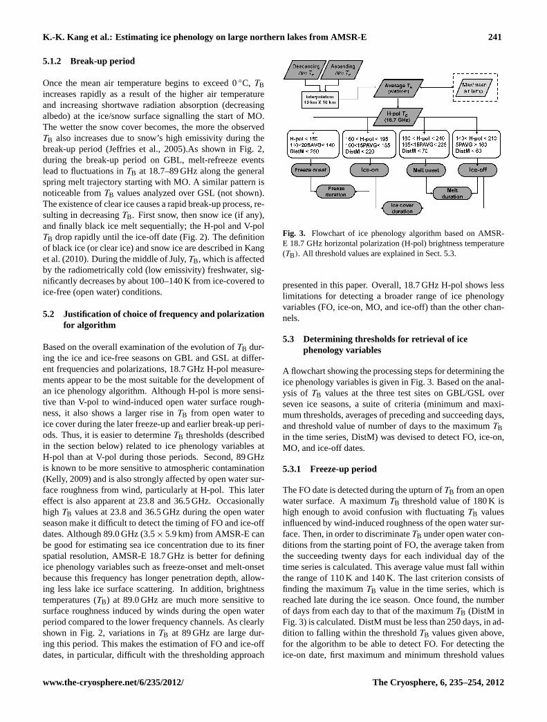
Fig. 3. Flowchart of ice phenology algorithm based on AMSR-E 18.7 GHz horizontal polarization (H-pol) brightness temperature(TB). All threshold values are explained in Sect. 5.3.

presented in this paper. Overall, 18.7 GHz H-pol shows lesslimitations for detecting a broader range of ice phenologyvariables (FO, ice-on, MO, and ice-off) than the other chan-nels.

5.3 Determining thresholds for retrieval of icephenology variables

A flowchart showing the processing steps for determining theice phenology variables is given in Fig. 3. Based on the anal-ysis of TB values at the three test sites on GBL/GSL overseven ice seasons, a suite of criteria (minimum and maxi-mum thresholds, averages of preceding and succeeding days,and threshold value of number of days to the maximumTBin the time series, DistM) was devised to detect FO, ice-on,MO, and ice-off dates.


The FO date is detected during the upturn ofTB from an openwater surface. A maximumTB threshold value of 180 K ishigh enough to avoid confusion with fluctuatingTB valuesinfluenced by wind-induced roughness of the open water sur-face. Then, in order to discriminateTB under open water con-ditions from the starting point of FO, the average taken fromthe succeeding twenty days for each individual day of thetime series is calculated. This average value must fall withinthe range of 110 K and 140 K. The last criterion consists offinding the maximumTB value in the time series, which isreached late during the ice season. Once found, the numberof days from each day to that of the maximumTB (DistM inFig. 3) is calculated. DistM must be less than 250 days, in ad-dition to falling within the thresholdTB values given above,for the algorithm to be able to detect FO. For detecting theice-on date, first maximum and minimum threshold values



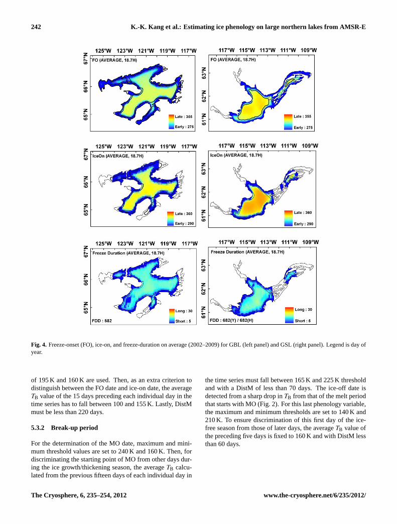
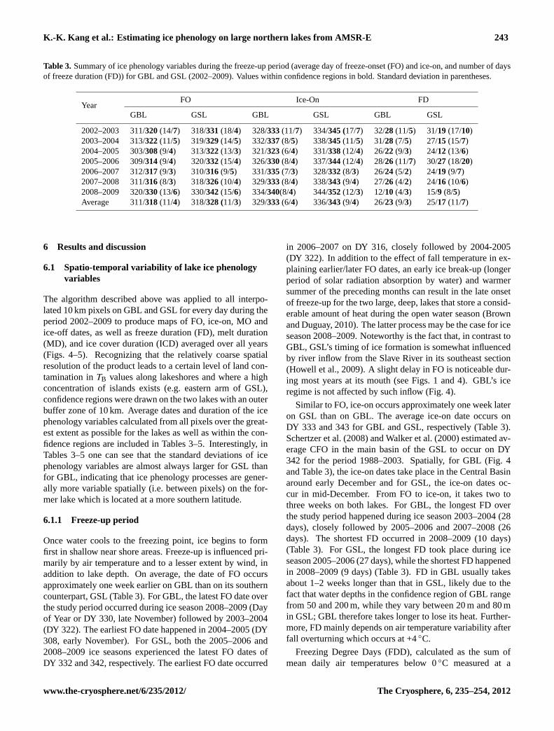
Fig. 4. Freeze-onset (FO), ice-on, and freeze-duration on average (2002–2009) for GBL (left panel) and GSL (right panel). Legend is day ofyear.

of 195 K and 160 K are used. Then, as an extra criterion todistinguish between the FO date and ice-on date, the averageTB value of the 15 days preceding each individual day in thetime series has to fall between 100 and 155 K. Lastly, DistMmust be less than 220 days.


For the determination of the MO date, maximum and mini-mum threshold values are set to 240 K and 160 K. Then, fordiscriminating the starting point of MO from other days dur-ing the ice growth/thickening season, the averageTB calcu-lated from the previous fifteen days of each individual day in

the time series must fall between 165 K and 225 K thresholdand with a DistM of less than 70 days. The ice-off date isdetected from a sharp drop inTB from that of the melt periodthat starts with MO (Fig. 2). For this last phenology variable,the maximum and minimum thresholds are set to 140 K and210 K. To ensure discrimination of this first day of the ice-free season from those of later days, the averageTB value ofthe preceding five days is fixed to 160 K and with DistM lessthan 60 days.



Table 3. Summary of ice phenology variables during the freeze-up period (average day of freeze-onset (FO) and ice-on, and number of daysof freeze duration (FD)) for GBL and GSL (2002–2009). Values within confidence regions in bold. Standard deviation in parentheses.

YearFO Ice-On FD

GBL GSL GBL GSL GBL GSL

2002–2003 311/320(14/7) 318/331(18/4) 328/333(11/7) 334/345 (17/7) 32/28 (11/5) 31/19 (17/10)2003–2004 313/322(11/5) 319/329(14/5) 332/337(8/5) 338/345(11/5) 31/28 (7/5) 27/15 (15/7)2004–2005 303/308(9/4) 313/322(13/3) 321/323(6/4) 331/338(12/4) 26/22 (9/3) 24/12 (13/6)2005–2006 309/314(9/4) 320/332(15/4) 326/330(8/4) 337/344(12/4) 28/26 (11/7) 30/27 (18/20)2006–2007 312/317(9/3) 310/316(9/5) 331/335(7/3) 328/332(8/3) 26/24 (5/2) 24/19 (9/7)2007–2008 311/316(8/3) 318/326(10/4) 329/333(8/4) 338/343(9/4) 27/26 (4/2) 24/16 (10/6)2008–2009 320/330(13/6) 330/342(15/6) 334/340(8/4) 344/352(12/3) 12/10 (4/3) 15/9 (8/5)Average 311/318(11/4) 318/328 (11/3) 329/333(6/4) 336/343(9/4) 26/23 (9/3) 25/17 (11/7)

6 Results and discussion

6.1 Spatio-temporal variability of lake ice phenologyvariables

The algorithm described above was applied to all interpo-lated 10 km pixels on GBL and GSL for every day during theperiod 2002–2009 to produce maps of FO, ice-on, MO andice-off dates, as well as freeze duration (FD), melt duration(MD), and ice cover duration (ICD) averaged over all years(Figs. 4–5). Recognizing that the relatively coarse spatialresolution of the product leads to a certain level of land con-tamination inTB values along lakeshores and where a highconcentration of islands exists (e.g. eastern arm of GSL),confidence regions were drawn on the two lakes with an outerbuffer zone of 10 km. Average dates and duration of the icephenology variables calculated from all pixels over the great-est extent as possible for the lakes as well as within the con-fidence regions are included in Tables 3–5. Interestingly, inTables 3–5 one can see that the standard deviations of icephenology variables are almost always larger for GSL thanfor GBL, indicating that ice phenology processes are gener-ally more variable spatially (i.e. between pixels) on the for-mer lake which is located at a more southern latitude.


Once water cools to the freezing point, ice begins to formfirst in shallow near shore areas. Freeze-up is influenced pri-marily by air temperature and to a lesser extent by wind, inaddition to lake depth. On average, the date of FO occursapproximately one week earlier on GBL than on its southerncounterpart, GSL (Table 3). For GBL, the latest FO date overthe study period occurred during ice season 2008–2009 (Dayof Year or DY 330, late November) followed by 2003–2004(DY 322). The earliest FO date happened in 2004–2005 (DY308, early November). For GSL, both the 2005–2006 and2008–2009 ice seasons experienced the latest FO dates ofDY 332 and 342, respectively. The earliest FO date occurred

in 2006–2007 on DY 316, closely followed by 2004-2005(DY 322). In addition to the effect of fall temperature in ex-plaining earlier/later FO dates, an early ice break-up (longerperiod of solar radiation absorption by water) and warmersummer of the preceding months can result in the late onsetof freeze-up for the two large, deep, lakes that store a consid-erable amount of heat during the open water season (Brownand Duguay, 2010). The latter process may be the case for iceseason 2008–2009. Noteworthy is the fact that, in contrast toGBL, GSL’s timing of ice formation is somewhat influencedby river inflow from the Slave River in its southeast section(Howell et al., 2009). A slight delay in FO is noticeable dur-ing most years at its mouth (see Figs. 1 and 4). GBL’s iceregime is not affected by such inflow (Fig. 4).

Similar to FO, ice-on occurs approximately one week lateron GSL than on GBL. The average ice-on date occurs onDY 333 and 343 for GBL and GSL, respectively (Table 3).Schertzer et al. (2008) and Walker et al. (2000) estimated av-erage CFO in the main basin of the GSL to occur on DY342 for the period 1988–2003. Spatially, for GBL (Fig. 4and Table 3), the ice-on dates take place in the Central Basinaround early December and for GSL, the ice-on dates oc-cur in mid-December. From FO to ice-on, it takes two tothree weeks on both lakes. For GBL, the longest FD overthe study period happened during ice season 2003–2004 (28days), closely followed by 2005–2006 and 2007–2008 (26days). The shortest FD occurred in 2008–2009 (10 days)(Table 3). For GSL, the longest FD took place during iceseason 2005–2006 (27 days), while the shortest FD happenedin 2008–2009 (9 days) (Table 3). FD in GBL usually takesabout 1–2 weeks longer than that in GSL, likely due to thefact that water depths in the confidence region of GBL rangefrom 50 and 200 m, while they vary between 20 m and 80 min GSL; GBL therefore takes longer to lose its heat. Further-more, FD mainly depends on air temperature variability afterfall overturning which occurs at +4◦C.

Freezing Degree Days (FDD), calculated as the sum ofmean daily air temperatures below 0◦C measured at a



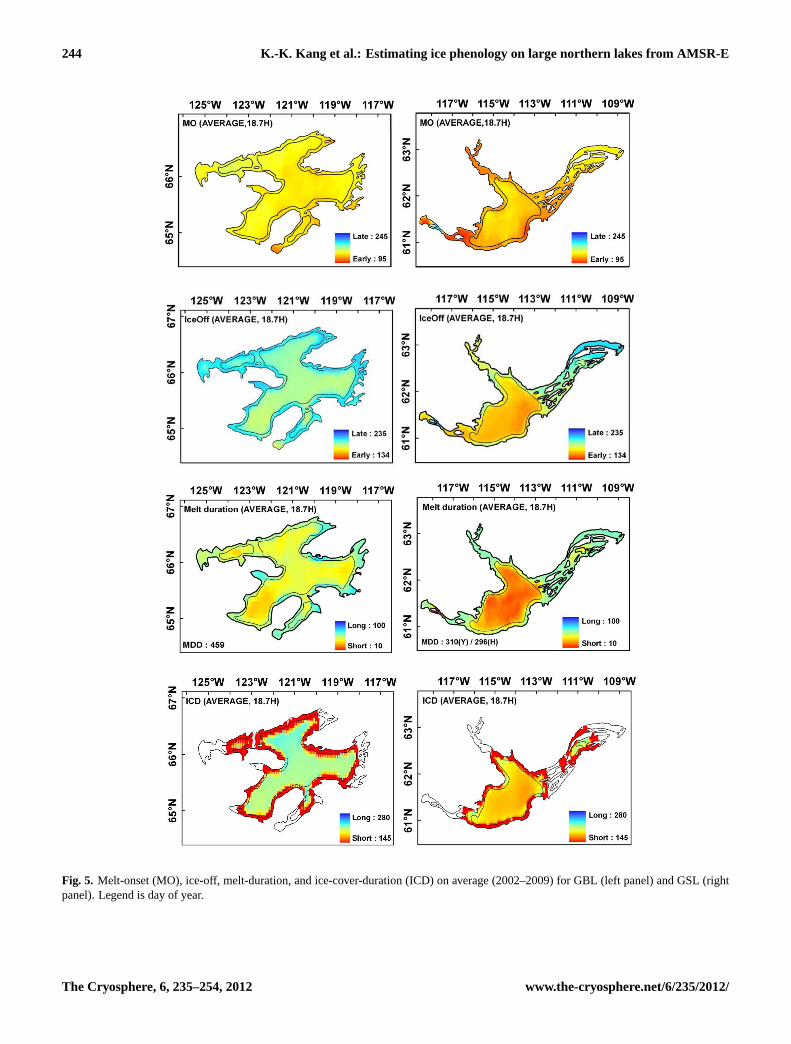
Fig. 5. Melt-onset (MO), ice-off, melt-duration, and ice-cover-duration (ICD) on average (2002–2009) for GBL (left panel) and GSL (rightpanel). Legend is day of year.



Table 4. Summary of ice phenology variables during the break-up period (average day of melt-onset (MO) and ice-off, and number of daysof melt duration (MD)) for GBL and GSL (2002-2009). Values within confidence regions in bold. Standard deviation in parentheses.

YearMO Ice-Off MD


2002–2003 133/127(14/12) 132/137(14/5) 193/183(14/7) 172/157(19/2) 61/55 (15/12) 41/19 (21/4)2003–2004 156/155(3/2) 147/150(16/6) 203/198(7/4) 186/169(20/4) 47/43 (7/4) 39/19 (19/7)2004–2005 133/132(11/7) 124/131(21/17) 193/186(11/4) 168/155(19/4) 60/54 (13/9) 44/24 (20/17)2005–2006 129/128(7/4) 119/122(9/5) 182/169(16/5) 161/140(21/6) 53/41 (16/7) 42/17 (22/7)2006–2007 142/141(10/6) 124/129(17/6) 197/187(12/6) 166/153(19/5) 55/46 (13/10) 42/24 (18/6)2007–2008 149/152(9/9) 133/135(16/10) 187/183(10/4) 170/156(20/2) 38/31 (13/8) 37/20 (20/9)2008–2009 167/168(8/7) 135/137(18/14) 200/197(6/3) 177/167(16/3) 33/28 (10/8) 42/30 (16/12)Average 144/143(6/3) 131/134(12/5) 194/186(9/3) 171/157(17/3) 50/43 (10/5) 41/22 (17/4)

Table 5. Summary of ice cover duration (ICDp) and open water season (OWS) (average number of days) for GBL and GSL (2002–2009).Values within confidence regions in bold. Standard deviation in parentheses. Note that OWS was not calculated for 2009 since it requiresice-on date to be known for fall freeze-up period 2009, which was not determined in this study.

YearICDp

YearOWS

GBL GSL GBL GSL

2002–2003 224/215(19/11) 195/220(28/29) 2003 123/116(23/22) 151/172(28/5)2003–2004 233/226(12/7) 203/223 (22/22) 2004 102/97(13/13) 130/154(28/6)2004–2005 232/229(10/7) 195/218 (20/22) 2005 119/112(16/16) 155/176(27/6)2005–2006 210/203(15/7) 176/201 (26/26) 2006 136/132(21/21) 156/177(26/7)2006–2007 225/217(14/8) 195/214(17/21) 2007 117/113(17/16) 155/172(24/7)2007–2008 219/215(10/6) 184/193(12/14) 2008 134/125(20/20) 162/186(30/6)2008–2009 230/223(11/5) 193/208(18/19)Average 225/218(9/6) 192/211(16/18) Average 122/116(15/14) 152/173(32/5)

meteorological station, and given in the bottom left of Fig. 4provide some indication of the effect of colder/warmer tem-peratures on FD. FDD calculated here between FO and ice-on date in each ice season. One should bear in mind, how-ever, that heat storage during the preceding open water sea-son will also have an impact on FD. Due to this, the relationbetween FDD and FD is not always consistent from year toyear for the two lakes.


The break-up process is primarily influenced by air tempera-ture variability, causing earlier or later MO dates on the twolakes. The MO dates mark the beginning of melt of snow onthe ice surface or the initiation of melt of ice in the case whena bare ice surface is encountered. Differences in the timing ofMO between GBL and GSL can largely be explained due tospring air temperature differences (Table 2). MO dates occurapproximately one week earlier on GSL than on GBL (Ta-ble 4). The average MO date occurs on DY 143 (end May) onGBL and DY 135 (mid May) on GBL (see Fig. 5). For GBL,

the earliest MO dates happened on DY 127 (2002–2003) andthe latest MO dates occurred in 2003–2004 (DY 155, earlyJune) (Table 4). For GSL, the earliest MO date occurred onDY 122 (early May) in 2005–2006 and the latest date tookplace in 2003–2004 (DY 150, early June). Earlier (later) MOdates appears to be related to warm (cool) spring air tem-perature (Table 2). The warmer average spring air tempera-ture (−7.8◦C and−1.0◦C for GBL and GSL, respectively)caused earlier MO dates to occur in ice season 2005–2006,while the colder spring of ice season 2003–2004 (−11.7◦Cand−7.6◦C for GBL and GSL, respectively) resulted in laterMO dates.

In contrast to MO, the average ice-off dates on GSL areabout four weeks earlier (DY 157 – early June) than on GBL(DY 183 – early July) (see Fig. 5). For GBL, the latest ice-offdate occurred during ice season 2003–2004 on DY 198 (midJuly). The earliest ice-off date occurred in 2005–2006 onDY 169 (mid June) (Table 4). For GSL, the 2003–2004 iceseason experienced the latest ice-off dates of DY 169 (midJune). The earliest ice-off date for this lake happened in2005–2006 on DY 140 (mid May) (Table 4). Early ice-off



dates lengthen the open water season during the high solarperiod in spring/summer, resulting in a longer period of solarradiation absorption by the lakes and, subsequently, higherlake temperatures in late summer/early fall due to larger heatstorage. Looking at specific ice cover seasons, the colderspring/early summer climate conditions of 2004 and 2009contributed to later break-up, while the warmest conditionsof 2006 influenced earlier break-up (Table 4). On GSL, ice-off dates are earlier in the majority of years at the mouthof the Slave River which brings warmer water as this riverflows from the south into the lake (see Fig. 5). For GBL,however, ice-off dates are not influenced by similar river in-flow such that melt generally proceeds gradually from themore southern (warmer) to the northern sections of the lake.Unlike MO, the larger difference in ice-off dates between thetwo lakes (about four weeks) can be explained by a combina-tion of thicker ice and colder spring/early summer conditionsat GBL which, as a result, requires a greater number of daysabove 0◦C to completely melt the ice.

The average melt duration (MD), which encompasses theperiod from MO to ice-off, takes two to five weeks longer onGBL than on GSL (Table 4). For GBL, the longest MD was55 days in 2002–2003 but was only 28 days in 2008–2009(Table 4). For GSL, the longest MD lasted 30 days in 2008–2009, whereas the shortest MD took 17 days in 2005–2006(Table 4). The length of the MD is mainly controlled by thecombination of end-of-winter maximum ice thicknesses andspring/early summer temperatures. In general, the thinnerthe ice is before melt begins and the warmer the temperatureconditions are between MO and ice-off, the shorter the MDlasts. One exception is the central basin of GSL, where MDis also influenced by the inflow of water from Slave Riverwhich helps to accelerate the break-up process in this lake.Melting Degree Days (MDD), calculated as the sum of meandaily air temperatures above 0◦C at a meteorological stationfrom MO until ice-off, provide some indication of the ef-fect of colder/warmer temperatures in spring/early summeron MD for each ice season (see bottom left corner of Fig. 5).Visually, a relation appears to exist between long/short MDand low/high MDD for GBL. Such a relation does not seemto be present for GSL, likely as a result of the inflow of waterfrom Slave River.

6.1.3 Ice cover duration

The average ice cover duration (ICD), which is calculatedas the number of days between ice-on and ice-off dates, isone week shorter for GSL than for GBL over the full pe-riod of analysis (DY 218 and 211 on average, respectively).However, the length of the ICD can differ by as much asfour to five weeks between the two lakes in some years. ForGBL, the longest ICD was 229 days in 2004–2005, while theshortest lasted 203 days (2005–2006). For GSL, the longestICD lasted 223 days (2003–2004), while the shortest was 193days (2007–2008) (Table 5). In GBL’s Smith Arm and Dease

Arm (northern section of lake), lake ice stays longer than inthe other arms, up until the middle (or end) of July (Fig. 5),particularly during the two cold winter seasons of 2003–2004and 2008–2009. For GSL, shorter ICD occurs at the mouth ofSlave River and near Yellowknife compared to the east armof the lake (Fig. 5). ICD is influenced by river inflow fromSlave River for the full period of study (2002–2009), as it hasa particularly large influence on ice-off dates (see Fig. 5).

6.2 Comparison of AMSR-E ice phenology variableswith other satellite-derived ice products

While the AMSR-E retrieval algorithm captures well the spa-tial patterns and seasonal evolution of ice cover on GBL andGSL over several ice seasons, estimated dates of the variousice phenology variables should be compared to those deter-mined from other approaches and with different satellite sen-sors whenever possible, as to provide at least a qualitativeassessment of the level of agreement with existing products.A detailed quantification of uncertainty (biases) of the vari-ous ice products is, however, beyond the scope of this paper.This is a topic that merits investigation in a follow-up studyencompassing a larger number of lakes.

6.2.1 Comparison with other pixel-based products

Tables 6–8 present summary statistics of ice phenology vari-ables estimated at the pixel level from AMSR-ETB (2002–2009) against those obtained with daily QuikSCAT (2002–2006; Howell et al., 2009) and NOAA/IMS products (2004–2009). Values in these tables are the averages and standarddeviations calculated from all pixels over the complete lakesand their main basin (confidence regions). IMS ice variablesconsist of ice-on/ice-off dates and ICDp, while QuikSCAT-derived variables are comprised of FO/MO/ice-off dates andICDp calculated from FO to ice-off dates. The complexnature of the freeze-up process has been reported to makethe distinction between FO and ice-on dates difficult fromanalysis of the temporal evolution of backscatter (σ ◦) fromQuikSCAT (Howell et al., 2009). This can be explained bythe fact that QuikSCAT-derived ice phenology variables areinfluenced by deformation features such as ice rafts, wind-roughened water in cracks, and ridge formation during thefreeze-up period, acting to increaseσ ◦. However, time se-ries of AMSR-ETB at 18.7 GHz (H-pol) can differentiate FOfrom ice-on dates (see Fig. 2) asTB is largely controlled bychanges in emissivity progressively from the radiometricallycold open water to the warmer ice-covered lake surface, andnot as much by lake ice surface roughness, during the freeze-up period.

FO dates as determined from AMSR-E are about one weekearlier on average (7–11 days for GBL; 1–8 days for GSL)than those derived with QuikSCAT when considering the two



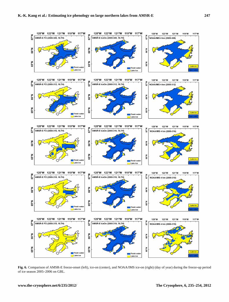
Fig. 6. Comparison of AMSR-E freeze-onset (left), ice-on (center), and NOAA/IMS ice-on (right) (day of year) during the freeze-up periodof ice season 2005–2006 on GBL.



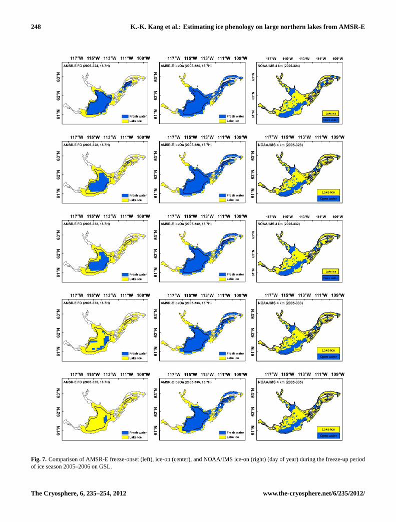
Fig. 7. Comparison of AMSR-E freeze-onset (left), ice-on (center), and NOAA/IMS ice-on (right) (day of year) during the freeze-up periodof ice season 2005–2006 on GSL.



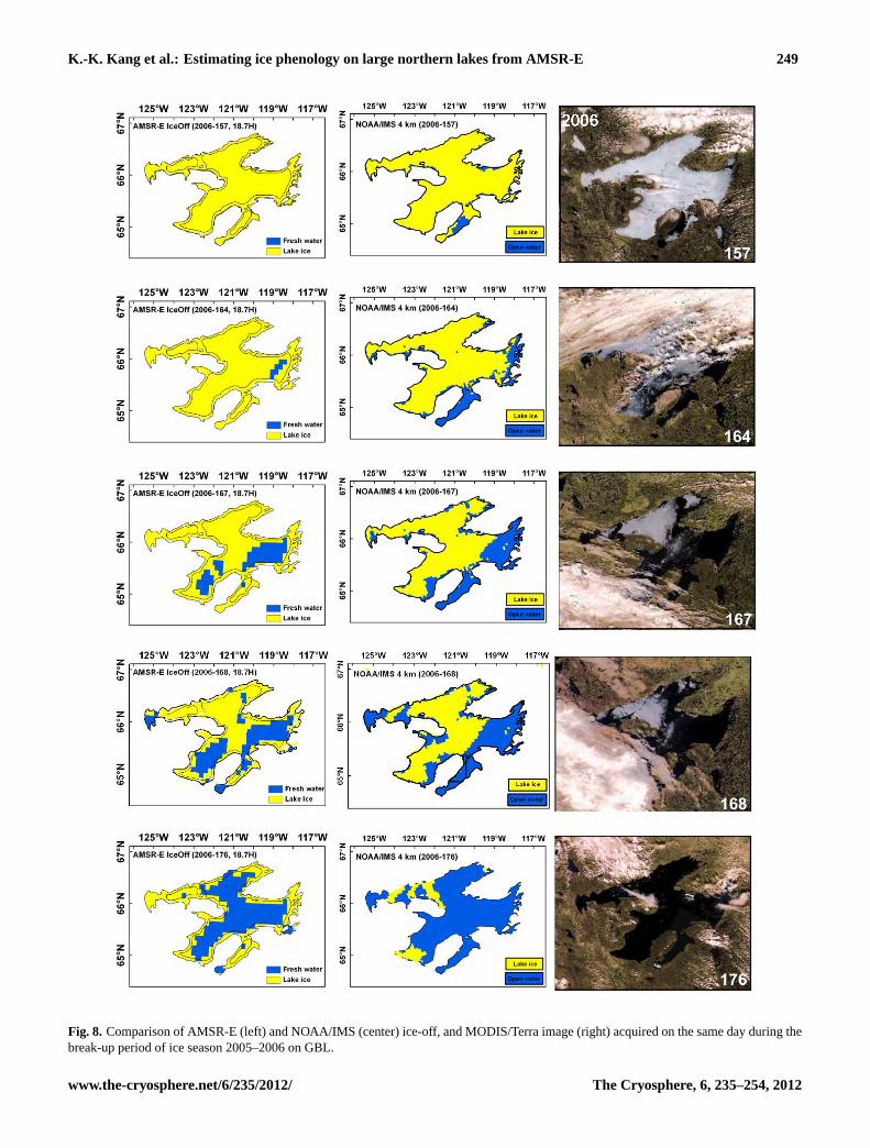
Fig. 8. Comparison of AMSR-E (left) and NOAA/IMS (center) ice-off, and MODIS/Terra image (right) acquired on the same day during thebreak-up period of ice season 2005–2006 on GBL.



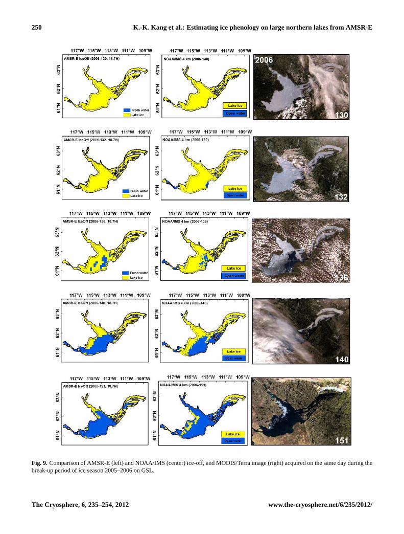
Fig. 9. Comparison of AMSR-E (left) and NOAA/IMS (center) ice-off, and MODIS/Terra image (right) acquired on the same day during thebreak-up period of ice season 2005–2006 on GSL.



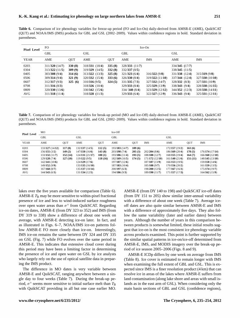
Table 6. Comparison of ice phenology variables for freeze-up period (FO and Ice-On) daily-derived from AMSR-E (AME), QuikSCAT(QUT) and NOAA/IMS (IMS) products for GBL and GSL (2002–2009). Values within confidence regions in bold. Standard deviation inparentheses.

Pixel LevelFO Ice-On

GBL GSL GBL GSL

YEAR AME QUT AME QUT AME IMS AME IMS

0203 311/320(14/7) 330 (8) 318/331 (18/4) 335 (8) 328/333 (11/7) 334/345 (17/7)0304 313/322(11/5) 309 (9) 319/329 (14/5) 332 (8) 332/337(8/5) 338/345 (11/5)0405 303/308(9/4) 314 (6) 313/322 (13/3) 325 (8) 321/323(6/4) 316/322(9/8) 331/338 (12/4) 315/319(9/8)0506 309/314(9/4) 321 (9) 320/332 (15/4) 333 (6) 326/330(8/4) 319/322(11/10) 337/344 (12/4) 327/330(10/10)0607 312/317(9/3) 325 (6) 310/316(9/5) 324 (5) 331/335(7/3) 327/332(14/7) 328/332 (8/3) 327/331(10/9)0708 311/316(8/3) 318/326 (10/4) 329/333(8/4) 325/329(13/9) 338/343 (9/4) 328/338(16/15)0809 320/330(13/6) 330/342 (15/6) 334/340(8/4) 323/329(12/12) 344/352 (12/3) 328/338(14/11)AVG 311/318(11/4) 318/328 (11/3) 329/333(6/4) 322/327(12/9) 336/343 (9/4) 325/331(12/11)

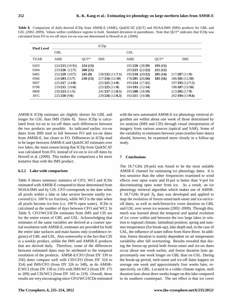
Table 7. Comparison of ice phenology variables for break-up period (MO and Ice-Off) daily-derived from AMSR-E (AME), QuikSCAT(QUT) and NOAA/IMS (IMS) products for GBL and GSL (2002–2009). Values within confidence regions in bold. Standard deviation inparentheses.

Pixel LevelMO Ice-Off

GBL GSL GBL GSL

YEAR AME QUT AME QUT AME QUT IMS AME QUT IMS

0203 133/127(14/12) 117 (8) 132/137(14/5) 112 (5) 193/183(14/7) 189 (6) 172/157(19/2) 163 (6)0304 156/155(3/2) 149 (2) 147/150(16/6) 143 (8) 203/198(7/4) 205 (3) 202/204(8/6) 186/169(20/4) 178 (5) 176/174(17/14)0405 133/132(11/7) 152 (14) 124/131(21/17) 100 (1) 193/186(11/4) 193 (5) 188/188(12/7) 168/155(19/4) 164 (7) 166/160(12/10)0506 129/128(7/4) 127 (10) 119/122(9/5) 118 (16) 182/169(16/5) 174 (5) 171/172(12/10) 161/140(21/6) 151 (11) 148/145(13/10)0607 142/141(10/6) 124/129(17/6) 197/187(12/6) 187/187(13/9) 166/153(19/5) 159/158(14/6)0708 149/152(9/9) 133/135(16/10) 187/183(10/4) 185/188(9/7) 170/156(20/2) 161/159(13/5)0809 167/168(8/7) 135/137(18/14) 200/197(6/3) 198/200(12/5) 177/167(16/3) 175/174(19/7)AVG 144/143(6/3) 131/134(12/5) 194/186(9/3) 189/190(11/7) 171/157(17/3) 164/162(15/9)

lakes over the five years available for comparison (Table 6).AMSR-ETB may be more sensitive to within-pixel fractionalpresence of ice and less to wind-induced surface roughnessover open water areas thanσ ◦ from QuikSCAT. Regardingice-on dates, AMSR-E (from DY 323 to 352) and IMS (fromDY 319 to 338) show a difference of about one week onaverage, with AMSR-E detecting ice-on later. In fact, andas illustrated in Figs. 6–7, NOAA/IMS ice-on patterns fol-low AMSR-E FO more closely than ice-on. Interestingly,IMS ice-on remains the same between DY 324 and DY 335on GSL (Fig. 7) while FO evolves over the same period inAMSR-E. This indicates that extensive cloud cover duringthis period may have been a limiting factor in determiningthe presence of ice and open water on GSL by ice analystswho largely rely on the use of optical satellite data in prepar-ing the IMS product.

The difference in MO dates is very variable betweenAMSR-E and QuikSCAT, ranging anywhere between a sin-gle day to four weeks (Table 7). During the break-up pe-riod, σ ◦ seems more sensitive to initial surface melt thanTBwith QuikSCAT providing in all but one case earlier MO.

AMSR-E (from DY 140 to 198) and QuikSCAT ice-off dates(from DY 151 to 205) show similar inter-annual variabilitywith a difference of about one week (Table 7). Average ice-off dates are also quite similar between AMSR-E and IMSwith a difference of approximately five days. They also fol-low the same variability (later and earlier dates) betweenyears. Although the number of years in this comparison be-tween products is somewhat limited, these initial results sug-gest that ice-on is the most consistent ice phenology variableacross products examined. This point is further supported bythe similar spatial patterns in ice-on/ice-off determined fromAMSR-E, IMS, and MODIS imagery over the break-up pe-riod of ice season 2005–2006 (Figs. 8 and 9).

AMSR-E ICDp differs by one week on average from IMS(Table 8). Ice cover is estimated to remain longer with IMSwhen examining the full extent of GBL and GSL. This is ex-pected since IMS is a finer resolution product (4 km) that canresolve ice in areas of the lakes where AMSR-E suffers fromland contamination (along lake shore and areas with small is-lands as in the east arm of GSL). When considering only themain basin sections of GBL and GSL (confidence regions),



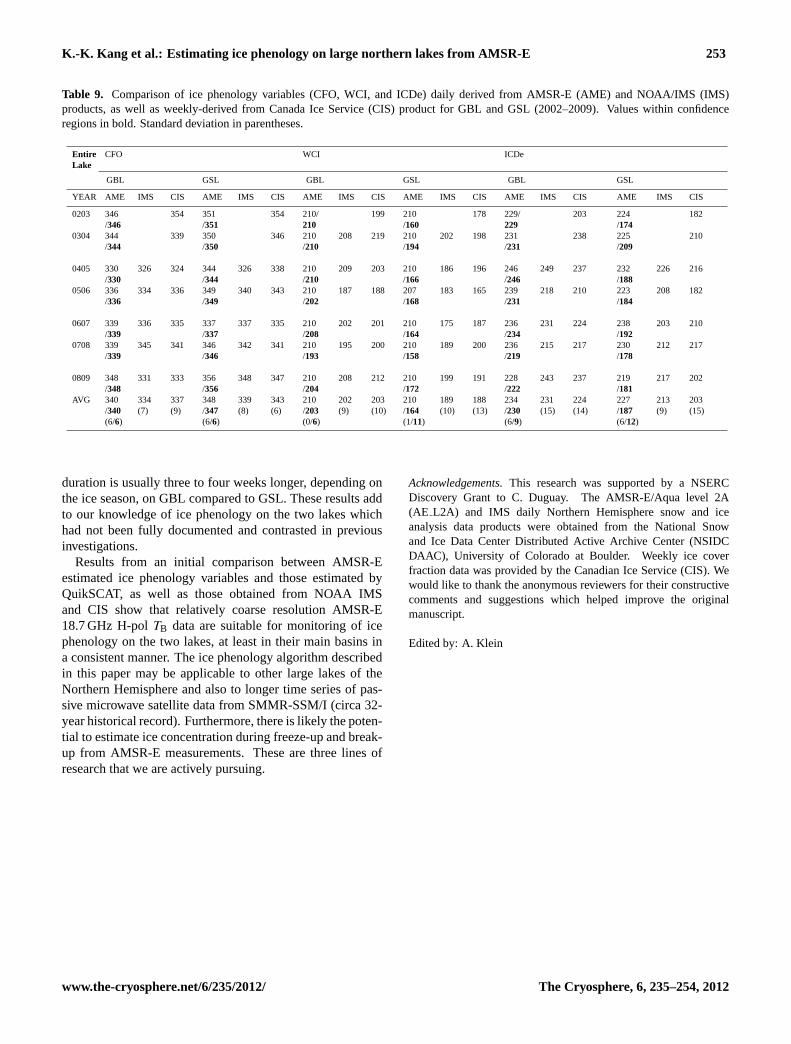
Table 8. Comparison of daily-derived ICDp from AMSR-E (AME), QuikSCAT (QUT) and NOAA/IMS (IMS) products for GBL andGSL (2002–2009). Values within confidence regions in bold. Standard deviation in parentheses. Note that QUT* indicates that ICDp wascalculated from FO to ice-off since ice-on was not determined in Howell et al. (2009).

Pixel LevelICDp

GBL GSL

YEAR AME QUT* IMS AME QUT* IMS

0203 224/215(19/11) 224 (13) 195/220 (28/29) 193 (12)0304 233/226 (12/7) 260 (11) 203/223 (22/22) 211 (12)0405 232/229 (10/7) 245 (9) 238/232(11/7.5) 195/218 (20/22) 205 (14) 217/207(11/9)0506 210/203(15/7) 218 (13) 217/216(12/10) 176/201 (26/26) 183 (16) 186/181(12/10)0607 225/217 (14/8) 225/221(14/8) 195/214 (17/21) 197/193(12/7.5)0708 219/215 (10/6) 225/225(11/8) 184/193 (12/14) 198/187(15/10)0809 230/223(11/5) 241/237(12/8.5) 193/208 (18/19) 213/202(17/9)AVG 225/218(9/6) 229/226(12/8.3) 192/211 (16/18) 202/194(13/9.6)

AMSR-E ICDp estimates are slightly shorter for GBL andlonger for GSL than IMS (Table 8). Since ICDp is calcu-lated from ice-on to ice-off dates such differences betweenthe two products are possible. As indicated earlier, ice-ondates from IMS tend to fall between FO and ice-on datesfrom AMSR-E, but closer to FO. Differences in ICDp tendto be larger between AMSR-E and QuikSCAT estimates overtwo lakes, the main reason being that ICDp from QuikSCATwas calculated from FO, instead of ice-on to ice-off dates byHowell et al. (2009). This makes the comparison a bit moretentative than with the IMS product.

6.2.2 Lake-wide comparison

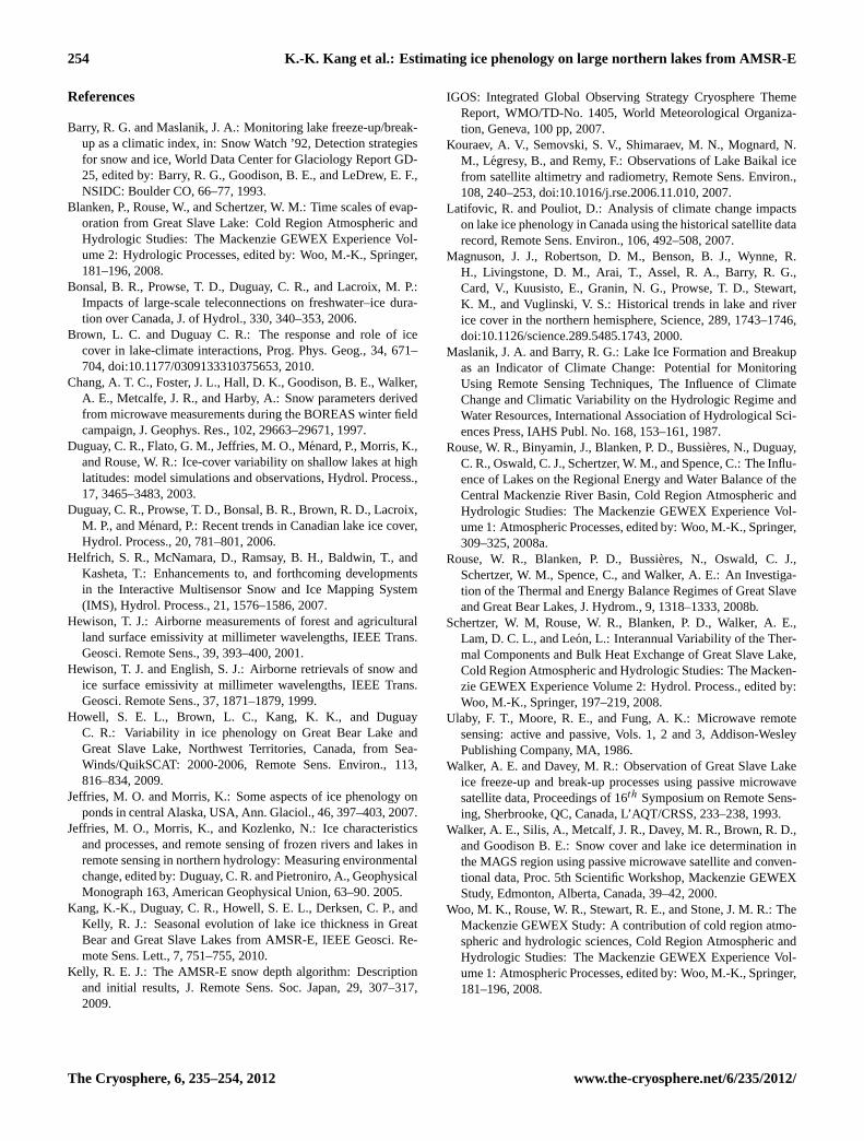
Table 9 shows summary statistics of CFO, WCI and ICDeestimated with AMSR-E compared to those determined fromNOAA/IMS and by CIS. CFO corresponds to the date whenall pixels within a lake or lake section become totally ice-covered (i.e. 100 % ice fraction), while WCI is the date whenall pixels become ice-free (i.e. 100 % open water). ICDe iscalculated as the number of days between CFO and WCI. InTable 9, CFO/WCI/ICDe estimates from IMS and CIS arefor the entire extent of GBL and GSL. Acknowledging thatestimates of the same variables are derived at a coarser spa-tial resolution with AMSR-E, estimates are provided for boththe entire lake surfaces and main basins only (confidence re-gions) of GBL and GSL. Also noteworthy is the fact that CISis a weekly product, unlike the IMS and AMSR-E productsthat are derived daily. Therefore, some of the differencesbetween estimated dates may be attributed to the temporalresolution of the products. AMSR-E/CFO (from DY 330 to356) dates compare well with CIS/CFO (from DY 324 to354) and IMS/CFO (from DY 326 to 348), as do AMSR-E/WCI (from DY 158 to 210) with IMS/WCI (from DY 175to 209) and CIS/WCI (from DY 165 to 219). Overall, theseresults are very encouraging since CFO/WCI/ICDe estimated

with the new automated AMSR-E ice phenology retrieval al-gorithm are within about one week of those determined byice analysts (IMS and CIS) through visual interpretation ofimagery from various sources (optical and SAR). Some ofthe variability in estimates between years (earlier/later dates)should, however, be examined more closely in a follow-upstudy.

7 Conclusions

The 18.7 GHz (H-pol) was found to be the most suitableAMSR-E channel for estimating ice phenology dates. It isless sensitive than the other frequencies examined to windeffects over open water and H-pol is better than V-pol fordiscriminating open water from ice. As a result, an icephenology retrieval algorithm which makes use of AMSR-E 18.7 GHz H-polTB data was developed and applied tomap the evolution of freeze-onset/melt-onset and ice-on/ice-off dates, as well as melt/freeze/ice cover duration on GBLand GSL over seven ice seasons (2002–2009). Through this,much was learned about the temporal and spatial evolutionof ice cover within and between the two large lakes in rela-tion to regional climate, latitudinal position, spring and sum-mer temperature (for break-up), lake depth and, in the case ofGSL, the influence of water inflow from Slave River. In addi-tion, freeze duration is mainly dependent on air temperaturevariability after fall overturning. Results revealed that dur-ing the freeze-up period both freeze-onset and ice-on datesoccur about one week earlier, and freeze duration lasts ap-proximately one week longer on GBL than on GSL. Duringthe break-up period, melt-onset and ice-off dates happen onaverage one week and approximately four weeks later, re-spectively, on GBL. Located in a colder climate region, meltduration lasts about three weeks longer on this lake comparedto its southern counterpart. The net effect is that ice cover



Table 9. Comparison of ice phenology variables (CFO, WCI, and ICDe) daily derived from AMSR-E (AME) and NOAA/IMS (IMS)products, as well as weekly-derived from Canada Ice Service (CIS) product for GBL and GSL (2002–2009). Values within confidenceregions in bold. Standard deviation in parentheses.

EntireLake

CFO WCI ICDe


YEAR AME IMS CIS AME IMS CIS AME IMS CIS AME IMS CIS AME IMS CIS AME IMS CIS

0203 346/346

354 351/351

354 210/210

199 210/160

178 229/229

203 224/174

182

0304 344/344

339 350/350

346 210/210

208 219 210/194

202 198 231/231

238 225/209

210

0405 330/330

326 324 344/344

326 338 210/210

209 203 210/166

186 196 246/246

249 237 232/188

226 216

0506 336/336

334 336 349/349

340 343 210/202

187 188 207/168

183 165 239/231

218 210 223/184

208 182

0607 339/339

336 335 337/337

337 335 210/208

202 201 210/164

175 187 236/234

231 224 238/192

203 210

0708 339/339

345 341 346/346

342 341 210/193

195 200 210/158

189 200 236/219

215 217 230/178

212 217

0809 348/348

331 333 356/356

348 347 210/204

208 212 210/172

199 191 228/222

243 237 219/181

217 202

AVG 340/340(6/6)

334(7)

337(9)

348/347(6/6)

339(8)

343(6)

210/203(0/6)

202(9)

203(10)

210/164(1/11)

189(10)

188(13)

234/230(6/9)

231(15)

224(14)

227/187(6/12)

213(9)

203(15)

duration is usually three to four weeks longer, depending onthe ice season, on GBL compared to GSL. These results addto our knowledge of ice phenology on the two lakes whichhad not been fully documented and contrasted in previousinvestigations.

Results from an initial comparison between AMSR-Eestimated ice phenology variables and those estimated byQuikSCAT, as well as those obtained from NOAA IMSand CIS show that relatively coarse resolution AMSR-E18.7 GHz H-polTB data are suitable for monitoring of icephenology on the two lakes, at least in their main basins ina consistent manner. The ice phenology algorithm describedin this paper may be applicable to other large lakes of theNorthern Hemisphere and also to longer time series of pas-sive microwave satellite data from SMMR-SSM/I (circa 32-year historical record). Furthermore, there is likely the poten-tial to estimate ice concentration during freeze-up and break-up from AMSR-E measurements. These are three lines ofresearch that we are actively pursuing.

Acknowledgements.This research was supported by a NSERCDiscovery Grant to C. Duguay. The AMSR-E/Aqua level 2A(AE L2A) and IMS daily Northern Hemisphere snow and iceanalysis data products were obtained from the National Snowand Ice Data Center Distributed Active Archive Center (NSIDCDAAC), University of Colorado at Boulder. Weekly ice coverfraction data was provided by the Canadian Ice Service (CIS). Wewould like to thank the anonymous reviewers for their constructivecomments and suggestions which helped improve the originalmanuscript.

Edited by: A. Klein



References

Barry, R. G. and Maslanik, J. A.: Monitoring lake freeze-up/break-up as a climatic index, in: Snow Watch ’92, Detection strategiesfor snow and ice, World Data Center for Glaciology Report GD-25, edited by: Barry, R. G., Goodison, B. E., and LeDrew, E. F.,NSIDC: Boulder CO, 66–77, 1993.

Blanken, P., Rouse, W., and Schertzer, W. M.: Time scales of evap-oration from Great Slave Lake: Cold Region Atmospheric andHydrologic Studies: The Mackenzie GEWEX Experience Vol-ume 2: Hydrologic Processes, edited by: Woo, M.-K., Springer,181–196, 2008.

Bonsal, B. R., Prowse, T. D., Duguay, C. R., and Lacroix, M. P.:Impacts of large-scale teleconnections on freshwater–ice dura-tion over Canada, J. of Hydrol., 330, 340–353, 2006.

Brown, L. C. and Duguay C. R.: The response and role of icecover in lake-climate interactions, Prog. Phys. Geog., 34, 671–704,doi:10.1177/0309133310375653, 2010.

Chang, A. T. C., Foster, J. L., Hall, D. K., Goodison, B. E., Walker,A. E., Metcalfe, J. R., and Harby, A.: Snow parameters derivedfrom microwave measurements during the BOREAS winter fieldcampaign, J. Geophys. Res., 102, 29663–29671, 1997.

Duguay, C. R., Flato, G. M., Jeffries, M. O., Menard, P., Morris, K.,and Rouse, W. R.: Ice-cover variability on shallow lakes at highlatitudes: model simulations and observations, Hydrol. Process.,17, 3465–3483, 2003.

Duguay, C. R., Prowse, T. D., Bonsal, B. R., Brown, R. D., Lacroix,M. P., and Menard, P.: Recent trends in Canadian lake ice cover,Hydrol. Process., 20, 781–801, 2006.

Helfrich, S. R., McNamara, D., Ramsay, B. H., Baldwin, T., andKasheta, T.: Enhancements to, and forthcoming developmentsin the Interactive Multisensor Snow and Ice Mapping System(IMS), Hydrol. Process., 21, 1576–1586, 2007.

Hewison, T. J.: Airborne measurements of forest and agriculturalland surface emissivity at millimeter wavelengths, IEEE Trans.Geosci. Remote Sens., 39, 393–400, 2001.

Hewison, T. J. and English, S. J.: Airborne retrievals of snow andice surface emissivity at millimeter wavelengths, IEEE Trans.Geosci. Remote Sens., 37, 1871–1879, 1999.

Howell, S. E. L., Brown, L. C., Kang, K. K., and DuguayC. R.: Variability in ice phenology on Great Bear Lake andGreat Slave Lake, Northwest Territories, Canada, from Sea-Winds/QuikSCAT: 2000-2006, Remote Sens. Environ., 113,816–834, 2009.

Jeffries, M. O. and Morris, K.: Some aspects of ice phenology onponds in central Alaska, USA, Ann. Glaciol., 46, 397–403, 2007.

Jeffries, M. O., Morris, K., and Kozlenko, N.: Ice characteristicsand processes, and remote sensing of frozen rivers and lakes inremote sensing in northern hydrology: Measuring environmentalchange, edited by: Duguay, C. R. and Pietroniro, A., GeophysicalMonograph 163, American Geophysical Union, 63–90. 2005.

Kang, K.-K., Duguay, C. R., Howell, S. E. L., Derksen, C. P., andKelly, R. J.: Seasonal evolution of lake ice thickness in GreatBear and Great Slave Lakes from AMSR-E, IEEE Geosci. Re-mote Sens. Lett., 7, 751–755, 2010.

Kelly, R. E. J.: The AMSR-E snow depth algorithm: Descriptionand initial results, J. Remote Sens. Soc. Japan, 29, 307–317,2009.

IGOS: Integrated Global Observing Strategy Cryosphere ThemeReport, WMO/TD-No. 1405, World Meteorological Organiza-tion, Geneva, 100 pp, 2007.

Kouraev, A. V., Semovski, S. V., Shimaraev, M. N., Mognard, N.M., Legresy, B., and Remy, F.: Observations of Lake Baikal icefrom satellite altimetry and radiometry, Remote Sens. Environ.,108, 240–253,doi:10.1016/j.rse.2006.11.010, 2007.

Latifovic, R. and Pouliot, D.: Analysis of climate change impactson lake ice phenology in Canada using the historical satellite datarecord, Remote Sens. Environ., 106, 492–508, 2007.

Magnuson, J. J., Robertson, D. M., Benson, B. J., Wynne, R.H., Livingstone, D. M., Arai, T., Assel, R. A., Barry, R. G.,Card, V., Kuusisto, E., Granin, N. G., Prowse, T. D., Stewart,K. M., and Vuglinski, V. S.: Historical trends in lake and riverice cover in the northern hemisphere, Science, 289, 1743–1746,doi:10.1126/science.289.5485.1743, 2000.

Maslanik, J. A. and Barry, R. G.: Lake Ice Formation and Breakupas an Indicator of Climate Change: Potential for MonitoringUsing Remote Sensing Techniques, The Influence of ClimateChange and Climatic Variability on the Hydrologic Regime andWater Resources, International Association of Hydrological Sci-ences Press, IAHS Publ. No. 168, 153–161, 1987.

Rouse, W. R., Binyamin, J., Blanken, P. D., Bussieres, N., Duguay,C. R., Oswald, C. J., Schertzer, W. M., and Spence, C.: The Influ-ence of Lakes on the Regional Energy and Water Balance of theCentral Mackenzie River Basin, Cold Region Atmospheric andHydrologic Studies: The Mackenzie GEWEX Experience Vol-ume 1: Atmospheric Processes, edited by: Woo, M.-K., Springer,309–325, 2008a.

Rouse, W. R., Blanken, P. D., Bussieres, N., Oswald, C. J.,Schertzer, W. M., Spence, C., and Walker, A. E.: An Investiga-tion of the Thermal and Energy Balance Regimes of Great Slaveand Great Bear Lakes, J. Hydrom., 9, 1318–1333, 2008b.

Schertzer, W. M, Rouse, W. R., Blanken, P. D., Walker, A. E.,Lam, D. C. L., and Leon, L.: Interannual Variability of the Ther-mal Components and Bulk Heat Exchange of Great Slave Lake,Cold Region Atmospheric and Hydrologic Studies: The Macken-zie GEWEX Experience Volume 2: Hydrol. Process., edited by:Woo, M.-K., Springer, 197–219, 2008.

Ulaby, F. T., Moore, R. E., and Fung, A. K.: Microwave remotesensing: active and passive, Vols. 1, 2 and 3, Addison-WesleyPublishing Company, MA, 1986.

Walker, A. E. and Davey, M. R.: Observation of Great Slave Lakeice freeze-up and break-up processes using passive microwavesatellite data, Proceedings of 16th Symposium on Remote Sens-ing, Sherbrooke, QC, Canada, L’AQT/CRSS, 233–238, 1993.

Walker, A. E., Silis, A., Metcalf, J. R., Davey, M. R., Brown, R. D.,and Goodison B. E.: Snow cover and lake ice determination inthe MAGS region using passive microwave satellite and conven-tional data, Proc. 5th Scientific Workshop, Mackenzie GEWEXStudy, Edmonton, Alberta, Canada, 39–42, 2000.

Woo, M. K., Rouse, W. R., Stewart, R. E., and Stone, J. M. R.: TheMackenzie GEWEX Study: A contribution of cold region atmo-spheric and hydrologic sciences, Cold Region Atmospheric andHydrologic Studies: The Mackenzie GEWEX Experience Vol-ume 1: Atmospheric Processes, edited by: Woo, M.-K., Springer,181–196, 2008.


http://dx.doi.org/10.1177/0309133310375653

http://dx.doi.org/10.1016/j.rse.2006.11.010

http://dx.doi.org/10.1126/science.289.5485.1743

Documents

Estimating ice phenology on large northern lakes - The Cryosphere