Embed Size (px)
Citation preview

Estimating Import Demand and Export Supply Elasticities∗
Hiau Looi Kee†
Alessandro Nicita‡
Marcelo Olarreaga§
January 2004 — Very Incomplete Draft
Abstract
The objective of this paper is to provide estimates of import demand and exportsupply elasticities for around 4200 goods (six digit of the Harmonized System) in 117countries. The empirical methodology follows the GDP function approach of Kohli(1991), which allows sufficient flexibility in terms of functional forms. Patterns foundin the estimated elasticities are discussed. The estimates and their standard errors canbe downloaded from a companion file.JEL classification numbers: F10, F11Keywords: Trade elasticities
∗We are grateful to Paul Brenton, Hadi Esfahani, Rob Feenstra, Joe Francois, Kishore Gawande, CatherineMann, William Martin, Christine McDaniel, Guido Porto, Claudio Sfreddo, Clinton Shiells, Dominique VanDer Mensbrugghe, and participants at a World Bank Seminar and the Empirical Trade Analysis Conferenceorganized by the Woodrow Wilson International Center for helpful comments and discussions. The viewsexpressed here are those of the authors and do not necessarily reflect those of the institutions to which theyare affiliated.
†Development Research Group, The World Bank, Washington, DC 20433, USA; Tel. (202)473-4155; Fax:(202)522-1159; e-mail: [email protected]
‡Development Research Group, The World Bank, Washington DC, 20433, USA; Tel. (202)458-7089; Fax:(202)522-1159; e-mail: [email protected]
§Development Research Group, The World Bank, Washington, DC 20433, USA, and CEPR, London,UK; Tel. (202)458-8021; Fax: (202)522-1159; e-mail: [email protected]

1 Introduction
Import demand and export supply elasticities are crucial inputs into many ex-ante analysis of
trade reform. For example, to evaluate the impact of regional trade agreements on trade flows
or customs revenue, one needs to first answer the question of how trade volumes would adjust
to changes in policies, for which we need both the import and export elasticities. To provide
estimates of overall protection including both tariff and non-tariff barriers one would need
first to transform non-tariff barriers into ad-valorem equivalents, for which import elasticities
are necessary. Moreover, if one needs to compare these overall levels of protection across
different countries to answer questions, for example, related to market access barriers faced
by developing country exporters, one would need to have a consistent set of trade elasticities,
estimated using the same data and methodology.1 These do not exist. The closest substitute
and the one often used by trade economists is the survey of the empirical literature put
together by Stern et al. (1976) more than 25 years ago. More recent attempts to provide
disaggregate estimates of trade elasticities (although not necessarily price elasticities, but
Armington or income elasticities) have been country specific and have mainly focused on
the United States. This include Shiells, Stern and Deardorff (1986), Shiells, Roland-Holst
and Reinert (1993), Blonigen and Wilson (1999), Marquez (1999, 2002, 2003), Broda and
Weinstein (2003) and Gallaway, McDaniel and Rivera (2003).
The objective of this paper is to fill in this gap by providing a set of consistent estimates
of import demand and export supply price elasticities for over 4200 products (at the 6 digit
of the Harmonized System) in more than 100 countries.2 The basic theoretical setup is the
production based GDP function approach as in Kohli (1991) and Harrigan (1997). Imports
and exports are considered as inputs and outputs of domestic production, for given exogenous
world prices, productivity and endowments. This GDP function approach takes into account
1For an attempt to measure these barriers using Anderson and Neary’s (2003) Multilateral Trade Re-strictiveness Index, see Kee, Nicita and Olarreaga (2004).
2To our knowledge the only set of estimates at the 6 digit level of the Harmonized System that exist inthe literature are the one provides by Panagariya et al. (2001) for the import demand elasticity faced byBangladesh exporters of apparel.

general equilibrium effects associated with the reallocation of resources due to exogenous
changes in prices or endowments, and thus has close links to trade theory. Moreover in a
world where a significant share of growth in world trade is explained by vertical specialization
(Yi, 2003), the fact that imports are treated as inputs into the revenue function —rather than
as final consumption goods as in most of the previous literature— seems an attractive feature
of this approach. While Kohli (1991) mainly focuses on aggregate import demand and
export supply functions and Harrigan (1997) on industry level export supply functions, this
paper modifies the GDP function approach to estimate good level import and export price
elasticities.
A total of 363777 import demand elasticities have been estimated (and around a similar
number of export supply elasticities will be estimated). The simple average across all coun-
tries and goods is about -4 and the median is -1.6. We found some interesting patterns in
our estimated import demand elasticities that are consistent with theory. First, homogenous
goods are shown to be more elastic than heterogenous goods. Second, there is evidence
indicating that import demand is more elastic when estimated at the good level rather than
the industry level. In other words, import demand elasticities decrease in magnitude as one
aggregates the level of observation. Third, large countries tend to have more elastic import
demands, due probability to a larger availability availability of domestic substitutes. Fourth,
more developed countries tend to have less elastic import demands, mainly driven by a higher
share of heterogenous goods in developed countries import demand. In sum, the estimated
import demand elasticities exhibit a significant variation across countries and products — a
nice property that has not been found in the existing literature.
Section 2 provides the theoretical framework, whereas section 3 describes the empirical
strategy. Section 4 discuss data sources. Section 5 discusses the results and provides some
patterns of trade elasticities across countries and goods. Section 6 concludes.
2

2 Theoretical Model — GDP Function Approach
The theoretical model follows Kohli’s (1991) GDP function approach for the estimation of
trade elasticities. We also draw on Harrigan’s (1997) treatment of productivity terms in
GDP functions. We will first derive the GDP, export supply and import demand functions
for one country. However, assuming that the GDP function is common across all countries
up to a country specific term —which controls for country productivity differences— it is then
easily generalized to a multi-country setting in the next section.
Consider a small open economy in period t.3 Let St ⊂ RN+M be the strictly convex
production set in t of its net output vector qt = (qt1, qt2, ..., q
tN ) and factor endowment vector
vt = (vt1, vt2, ..., v
tM) ≥ 0. For the elements in the net output vector qt, we adopt the con-
vention that positive numbers denote outputs, which include exports, and negative numbers
denote inputs, which include imported goods. We consider outputs for export as different
products as output for domestic market. This could be motivated by higher product standard
requirements in international markets.
Given the exogenous price vector pt = (pt1, pt2, ..., p
tN) > 0, perfect competition of firms
would lead the economy to produce at a mixed of goods that maximizes its GDP in each
period t :
Gt pt, vt ≡ maxqt
pt · qt : qt, vt ∈ St . (1)
Thus the GDP function, Gt (pt, vt) , is the maximum value of goods the economy can produce
given exogenous prices, its factor endowments and technology in period t. It equals to the
total value of output for exports and domestic consumption, minus the total value of imports
(qtn < 0 for imports).
Assuming that production of each output n in period t is affected by some good specific
(and later on country specific) Hicks-neutral productivity level, Atn, such that we can define
qt = (qt1, qt2, ..., q
tN) as the net output vector in t that is net of any Hicks-neutral productivity
3For a discussion of the relevance of the small country assumption when estimating trade elasticities, seeRiedel (1988), Athukorala and Riedel (1994) and Panagariya et al. (2001).
3

gains:
qtn = Atnqtn, ∀n = 1, ..., N.
Define At = diag {At1, At2, ..., AtN} , a N -dimensional diagonal matrix, then we can re-expressEquation (1) as
Gt ptAt, vt ≡ maxqt
ptAt · qt : qt, vt ∈ St ⇒
Gt pt, vt = maxqt
pt · qt : qt, vt ∈ St (2)
with pt = (pt1, pt2, ..., p
tN) and S
t ⊂ RN+M is the product set that is defined over (qt, vt) .
The advantage to differentiate qtn and qtn is that the latter recognizes that productivity level
is exogenous to the economy.4 One way to interpret the multiplicative relationship of good
prices and the associated productivity level is to define
ptn ≡ ptnAtn (3)
as the productivity augmented price level of good n. This will be a useful addition in our
empirical application as unit prices for the same tariff line will vary across different countries,
which will then be explained by differences in productivity in different countries. In a recent
study, Schott (forthcoming) successfully explains variation in unit value for similar products
in different countries with GDP per capita levels. To the extent that GDP per capita is
a proxy for labor productivity Schott’s finding provides some evidence on our productivity
augmented price level, pt.
GDP function, Gt (pt, vt) , is homogeneous of degree one respect to good prices. Strictly
convexity of St also ensures that the second order sufficient conditions are satisfied, such
that Gt (pt, vt) is twice differentiable and it is convex in pt and concave in vt. By Envelope
Theorem, the gradient of Gt (pt, vt) with respect to pt is the unique output supply functions
4It could depend on past economic activities, such as lagged value of capital investment or R&D activities,but at the moment when firms are facing production choices, it is nevertheless considered as given.
4

of the economy in period t :
∂Gt (pt, vt)
∂ptn= qtn pt, vt , ∀n = 1, ..., N. (4)
Equation (4) implies that an increase in the price of exports would lead to an increase in GDP
in period t, while an increase in import prices would reduce GDP in period t. Given that
Gt (pt, vt) is continuous and twice differentiable, and is convex and homogeneous of degree
one with respect to prices, Euler Theorem also implies that the output supply functions,
Equation (4), are homogenous of degree zero in prices, have non-negative own substitution
effects and have symmetric cross substitution effects:
∂2Gt (pt, vt)
∂ptn∂pti
=
∂qtn(pt,vt)
∂ptn≥ 0, ∀n = i
∂qtn(pt,vt)∂pti
=∂qti(pt,vt)
∂ptn, ∀n = i
. (5)
In other words, for every final good, including exports, an price increase raises output supply;
for every input, including imports, an increase in prices decreases the demand of the input.
In addition, an increase in the price of an imported input causes supply of an exported
output to decrease, and an increase in the price of the exported output would increase the
demand of the imported input in the same magnitude.
Thus with a well defined GDP function we could derive both the export supply functions
and import demand functions, and as long as GDP function is twice differentiable, we could
also derive the own and cross partial effects of exports and imports, and hence the export
supply and import demand elasticities.
To implement the above GDP function empirically, let’s assume, without loss of gener-
ality, that Gt (pt, vt) follows a flexible translog functional form with respect to prices and
5

endowments:
lnGt pt, vt = at00 +N
n=1
at0n ln ptn +
1
2
N
n=1
N
k=1
atnk ln ptn ln p
tk
+M
m=1
bt0m ln vtm +
1
2
M
m=1
M
l=1
btml ln vtm ln v
tl
+N
n=1
M
m=1
ctnm ln ptn ln v
tm, (6)
where all the translog parameters a, b and c s are indexed by t to allow for changes over time.
In order to make sure that Equation (6) satisfies the homogeneity and symmetry properties
of a GDP function, we impose the following restrictions:
N
n=1
at0n = 1,N
k=1
atnk =N
n=1
ctnm = 0, atnk = a
tkn, ∀n, k = 1, ..., N, ∀m = 1, ...,M. (7)
Furthermore, if we assume that the GDP function is homogeneous of degree one in factor
endowments, then we also need to impose the following restrictions:
N
n=1
bt0n = 1,N
k=1
btnk =M
m=1
ctnm = 0, btnk = b
tkn, ∀n, k = 1, ...,N, ∀m = 1, ...,M. (8)
Given the translog functional form and the symmetry and homogeneity restrictions, the
derivative of lnGt (pt, vt) with respect to ln ptn gives us the share in GDP of good n at period
t :
stn pt, vt = at0n +N
k=1
atnk ln ptk +
M
m=1
ctnm ln vtm
= at0n + atnn ln p
tn +
k=n
atnk ln ptk +
M
m=1
ctnm ln vtm, ∀n = 1, ..., N, (9)
with stn > 0 denoting the share of output of good n in GDP at time t, and stn < 0 denotes
share of import of good n in GDP in period t. From the above equation it could be shown
6

that if good n is an exported output, then the export supply elasticity of good n is
εtn ≡∂ ln qtn (p
t, vt)
∂ ln ptn=atnnstn+ stn − 1 ≥ 0, ∀stn > 0, (10)
with atnn ≥ stn (1− stn), ensuring that the price elasticity of export supply is non-negative(i.e., curvature conditions of the GDP function are satisfied to ensure GDP maximization).
Similarly, if good n is an imported good, then the import demand elasticity of good n is
εtn ≡∂ ln qtn (p
t, vt)
∂ ln ptn=atnnstn+ stn − 1 ≤ 0, ∀stn < 0, (11)
with atnn ≥ stn (1− stn), where (−qtn) > 0 denotes the quantity demanded of imports.5 A niceproperty of this import demand elasticities from a trade theory point of view is that they are
estimated keeping import prices and endowments constant —and not income as in the more
usual log linear estimation (see Kohli, 1991, section 5.3 for a thorough discussion). Notice
that for small |stn| , the size of the import elasticity, εtn, depends on the sign of atnn:
εtn
< −1 if atnn > 0,= −1 if atnn = 0,> −1 if atnn < 0.
This result is highly intuitive. If the share of imports in GDP is fixed (atnn = 0) with respect
to the price of import, then the implied import demand is unitary elastic such that an
increase in import price induces an equi-proportional decrease in import quantities and
leaves the value of imports unchanged. If the share of imports in GDP, which is negative
by construction, decreases with import price (atnn < 0) , i.e., −ptnqtn > 0 increases with ptn,then the implied import demand is inelastic, so that an increase in import price induces a
5Let ztn > 0 be the quantity imported of good n in period t, and let qtn = −ztn < 0, then
εtn ≡∂ ln ztn∂ ln ptn
=∂ztn∂ptn
ptnztn=
∂qtn∂ptn
ptnqtn=
∂ ln qtn∂ ln ptn
≤ 0.
7

less than proportionate decrease in import quantities. Finally, if the share of import in GDP
increases with import prices (atnn > 0) , then the implied import demand must be elastic
such that an increase in the price of import induces a more than proportionate decrease in
import quantity.6
Cross-price elasticities for import demand and export supply can be calculated in a similar
fashion:
εtn,k ≡∂ ln qtn (p
t, vt)
∂ ln ptk=atnkstn+ stk, ∀n, k. (12)
Finally, given that the elasticities are linear in the estimated coefficients, it is also possible to
perform hypothesis testing on significance of the elasticities, base on the regression standard
errors of ann :
S.E. εtnc =S.E. (ann)
stnc, ∀n.
Notice that by the design of the model, the estimated elasticities vary by good, country and
year, since stnc varies along all these dimensions.
3 Empirical Strategy
With data on output shares, unit values and factor endowments, Equation (9) is the basis
of our estimation of export and import elasticities, over a panel of countries and years for
each good. In principle, we could first estimate the own substitution effects, atnn, for every
good according to Equation (9) , and apply Equations (10) and (11) to derive the implied
estimated elasticities, since the own price elasticity is a linear function of own partial effects.
However, there are literally thousands of goods traded among the countries in any given year.
Moreover, on top of the thousands of traded commodities, there are even more non-traded
commodities that also utilize countries’ factor endowments and contribute to GDP in each
6Kohli (1991) found an inelastic demand for the aggregate US imports with ann < 0, while highly elasticdemand for the durables and services imports of the US, with the corresponding ann > 0, when the aggregateimport is broken down into 3 disaggregate groups.
8

country. Thus the number of explanatory variables in Equation (9) could easily exhausts
our degrees of freedom or introduce serious collinearity problems.
Given that our objective is to estimate the own price effect, atnn, for every good n, we
re-express the multiple goods GDP function approach into a “two-good economy” producing
goods n and −n :
Gt ptn, pt−n, v
t ≡ maxqt
ptnqtn + p
t−nq
t−n : q
t, vt ∈ St , (13)
where for every good n, we define pt−nqt−n =
N
k=n,k=1
ptkqtk as the part of GDP that is originated
from all other goods the economy produces. Provided that we have knowledge of the price
of good −n, the translog specification of Equation (13) and the implied share equations forgood n could then be applied to estimate the own price effect of every good n in this two good
economy in a strict forward fashion with homogeneity and symmetry constraints imposed:
lnGt ptn, pt−n, v
t = at00 + at0n ln p
tn + a
t0−n ln p
t−n
+1
2atnn ln ptn
2+1
2at−n−n ln pt−n
2+ atn−n ln p
tn ln p
t−n
+M
m=1
bt0m ln vtm +
1
2
M
m=1
M
l=1
btml ln vtm ln v
tl
+M
m=1
ctnm ln ptn ln v
tm +
M
m=1
ct−nm ln pt−n ln v
tm, (14)
stn ptn, pt−n, v
tc = at0n + a
tnn ln
ptnpt−n
+M
m=1,m=k
ctnm lnvtmvtk, ∀n, c, t. (15)
To obtain pt−n, we need to impose more structure to the model. According to Caves,
Christensen and Diewert (1982), if Gt (pt, vt) follows a translog functional form as shown
in Equation (6) or (14)and assuming that all the translog parameters are time invariant,
9

atnk = ank, ∀n, k, t, then a Tornqvist price index,
PT pt, pt−1, vt, vt−1 ≡N
n=1
ptnpt−1n
12(stn+s
t−1n )
, (16)
is the exact price index for Gt (pt, vt) , and is equal to the geometric mean of the theoretical
GDP price index P t (pt, pt−1, vt−1) ≡ Gt−1(pt,vt−1)Gt−1(pt−1,vt−1) and P
t (pt, pt−1, vt) ≡ Gt(pt,vt)Gt(pt−1,vt) . Thus, in
a two-good economy, the overall GDP deflator is the weighted average between the price
changes of good n and the composite good −n :
lnPT pt, pt−1, vt, vt−1 =1
2stn + s
t−1n ln
ptnpt−1n
+1
2st−n + s
t−1−n ln
pt−npt−1−n
. (17)
In other words, with information on the overall GDP deflator and the unit value of good n,
we could infer the underlying price index of good −n, through Equation (17) . Specifically,we can re-write Equation (17) to show that the change in the price index of the composite
good −n is the difference between the change in the overall GDP deflator of period t andthe weighted change in the price of good n :
lnpt−npt−1−n
=1
12st−n + s
t−1−n
lnPT pt, pt−1, vt, vt−1 − 12stn + s
t−1n ln
ptnpt−1n
,
ln pt−n = ln pt−1−n +1
12st−n + s
t−1−n
lnPT pt, pt−1, vt, vt−1 − 12stn + s
t−1n ln
ptnpt−1n
.(18)
Thus, by normalizing prices of all goods, both n and −n, to 1 in the first year of our sample,we would be able to construct both price indexes for good n and −n for each sample countryc.
We estimate Equation (9) across countries and years and assume that the parameters
of the GDP function are time invariant as required by the Tornqvist price index. Country
subscript c is introduced to highlight the panel dimension in the estimation:
stnc ptnc, p
t−nc, v
tc = at0n + a0nc + ann ln
ptncpt−nc
+
M
m=1,m=k
cnm lnvtmcvtkc, ∀n, c, t. (19)
10

Notice that even though we assume that ann is common across all countries, the implied
own price elasticities will still vary across countries, given that stn is good, time and country
specific (see Equations (11) and (10)). Equation (15) allows for country and year specific-
effects for the constant term, which allows us to capture the shift in the GDP function that
is due to productivity. We also impose homogeneity constraints with respect to endowments
by setting m cnm = 1 (i.e., all the endowment variables are measured relative to land
endowment, vk). Notice that in this two-good economy set up, there is a system of two
equations for each good, one for n and one for −n. To avoid singularity in the estimation,we drop the equation for −n such that no cross equation restrictions are necessary, and theestimation procedure is reduced to a single equation estimation. Also, note that separability
is not imposed on the estimation —contrary to much of the existing literature— as the price
of any other good −n affects imports through the Tornqvist price index of −n. As arguedby Winters (1984) separability is rarely observed in the data.7
For Equation (19) to be the first order condition of the GDP maximization program,
second order conditions need to be satisfied (the Hessian matrix needs to be negative semi-
definite). Such conditions are also known as the curvature conditions which ensure that
the GDP function is smooth, differentiable, and convex with respect to output prices and
concave with respect to input prices and endowments. This requires that the estimated
export elasticities are positive and import elasticities are negative for all observations (see
Equation (5)). Note that for a given good n, the estimated import elasticities are all negative,
if the following condition holds:
ann ≥ stnc 1− stnc , ∀c, t.
Given that by construction stnc < 0 for imports and stnc > 0 for exports, the above is true if
ann ≥ sn (1− sn) , (20)
7Note that we do impose non-jointness in production. For a discussion of separability, see chapter 4 inKohli (1991).
11

where sn is the maximum (negative for imports, positive for exports) share in the sample for
good n. Denote all the variables of such an observation (country) with an over-bar. We then
difference Equation (19) with respect to this observation, where the curvature condition is
most likely to be violated:
stnc ptnc, p
t−nc, v
tc = a0n + at0n − at0n + (a0nc − a0n) + ann ln
ptncpt−nc
− ln pnp−n
+M
m=1,m=k
cnm lnvtmcvtkc− ln vm
vk. (21)
Notice that differencing with respect to this observation does not affect the slope coefficients,
ann and cnm, while the estimated constant term, a0n, now has the interpretation of sn, by
construction. In addition, each country-year specific effect represents the differences in the
average import or export share of country c at time t and sn.
To impose a non-negative constraint such as Equation (20) , we reparameterize Equation
(21)as follows;8
ann = τ2nn + a0n (1− a0n) ,
where a0n and τ are the parameters to be estimated nonlinearly. Thus, the final version of
the share equation is:
stnc ptc, v
tc = a0n + at0n − at0n + (a0nc − a0n) + τ 2nn + a0n − a20n ln
ptncpt−nc
− ln pnp−n
+M
m=1,m=k
cnm lnvtmcvtkc− ln vm
vk+ utnc, (22)
where a neoclassical regression error term, utnc, is included to control for measurement error
in the aggregate GDP deflator which is used to construct ln pt−nc. Given that a0n and τ is
nonlinear with respect to utnc, nonlinear estimation techniques are necessary.
8Note that the imposition of the curvature conditions is binding in only 10 percent of the observationsin our sample, but in order to ensure comparability in the estimation procedure we estimate all elasticitiesusing the same methodology.
12

4 Data
The basic data consists of exports and imports data reported by different countries to the
UN Comtrade system at the 6 digit of the Harmonized System (HS —around 4200 products).
This data provides both value and volumes of exports and imports for each country allowing
to calculate unit values. It is available at the World Bank through the World Integrated
Trade System (WITS). The Harmonized System was introduced in 1988, but a wide use of
this classification system only started in the mid 1990s. So the basic data will consist of an
unbalanced panel of exports and imports for around 100 countries at the 6 digit level of the
HS for the period 1988-2002. The number of countries will obviously vary from product to
product depending on how many countries export or import the product and when different
countries started reporting their trade statistics using the HS.
We use year dummies to control for the year specific effects. As for country specific effects,
for the OECD countries in the sample, we employ country dummies, while the developing
countries in the sample are aggregated into the 9 World Bank main geographic regions and
regional dummies are used. This is to save some degree of freedom given the complicated
nature of the nonlinear estimation. In addition, relative GDP per capita (relative to the GDP
per capita of the observation where the curvature condition is more likely to be violated) is
also introduced as additional country controls.
Data on GDP per capita, labor force, agriculture land, and the GDP deflator series are
all from World Development Indicators (WDI, 2003). Data on capital endowments available
in Feenstra and Kee (2004), which is constructed using perpetual inventory method based
on real investment data in WDI (2003).
5 Empirical Results
We first discuss the results obtained for the estimation of import demand elasticities and
then we turn to the estimates of export supply price elasticities.
13

5.1 Import Demand Elasticities
Given the lack of existing estimates on these good level elasticities, we need some guidelines
from theory to judge our results:
1. The import demand for homogenous goods is more elastic than for heterogenous goods.
Rauch (1999) classifies goods into these two categories, which we can use to test this
hypothesis.
2. Import demand is more elastic at the disaggregate level — the substitution effect be-
tween cotton shirts and wool shirts is larger than the substitution effect between shirts
and pants, or garment and electronics. Thus, we expect the HS 6 digit good level im-
port demand elasticities estimates to be larger in magnitude (more negative) than HS
4 digit and HS 2 digit estimates. Broda and Weinstein (2004) uses a similar guideline
for their elasticities of substitution estimates.
3. Import demand is more elastic in large countries. In large countries there is a larger
range of domestically produced goods and therefore the sensitivity to import prices of
import demand is expected to be larger. In other words, it is easier to substitute away
from imports into domestically produced goods in large economies.
4. Import demand is less elastic in more developed countries. The relative demand for
heterogenous goods is probably higher in rich countries. Given that heterogenous goods
are less elastic, we expect the import demand to be less elastic in rich countries.
We will test our estimates against the above hypotheses. At HS 6 digit good level,
we estimate a total of 363,777 import demand elasticities. The simple average across all
countries and goods is -3.96 and the standard deviation is 7.88 suggesting quite a bit of
variance in the estimates. Figure 1 shows the Kernel density estimate of the distribution of
all estimated elasticities. The red line to the left denotes the sample mean (-3.96), and the
line to the right is the sample median (-1.57).
14

All import demand elasticities are quite precisely estimated. The average t-statistics is
around -14.4 which shows that our estimates are highly significant. The median t-statistics
is around -2.7. Around 20 percent of the observations have t-statistics greater than -2,
suggesting that the elasticities have not been very precisely estimated in those cases.
The estimates vary quite significantly across countries. The top three countries with
the highest average elasticity across products are Japan, India and the United States with
average import demand elasticities of -9.15, -7.71 and -7.43, respectively. The three countries
with the lowest average import demand elasticities are Surinam, Maldives and Guyana with
averages of -1.24, -1.54 and -1.60 respectively. Table 1 provides several moments of the
estimated import demand elasticities by country: the simple average, the standard deviation,
the median and the import-weighted average elasticity.
Figure 2 presents the Kernel density estimates of the distributions of import demand
elasticities of Metal (HS 72-83) and Machinery (HS 84-89). Given that Metal products are
expected to be more homogenous than Machinery, we see this as a first test into the ho-
mogeneity vs heterogeneity question (tests based on Rauch, 1999 will follow). The average
import elasticity of Metal is -1.70 while it is —1.58 for Machinery. A simple mean test sup-
ported the hypothesis that Metal import demand is more elastic than that of the Machinery,
with a t-statistics of -4.33. Thus we found support that homogenous goods tend to be more
elastic than heterogenous goods.
Figures 3 and 4 jointly test the last two hypotheses that import demand is more elastic
in large and less developed countries, by regressing the median import elasticities on log of
GDP and log of GDP per capita. It is clear that both hypotheses cannot be rejected.
Finally, we estimated import demand elasticities, but aggregating our data at the 4 and
2 digit level of the Harmonized System, as well as at the aggregate level. Table 3 illustrates
the average elasticities obtained at different levels of aggregation. Note that in principle the
aggregated import demand elasticities should be equal to the import-weighted averages. We
therefore also calculated the aggregate elasticities using import-weights at the 4 and 2 digit.
We correlated the calculated and estimated series and obtained the following correlation
15

coefficients XX, YY, ZZ.
5.2 Export supply price elasticities
...................
6 Concluding Remarks
This paper provides a methodology to estimate import demand and export supply price
elasticities for a wide variety of countries at the six digit level of the Harmonized System
(more than 4200 tariff lines), that can be implemented with existing trade data.
Sample average of the estimated import demand elasticities at HS 6 digit is about -4,
while the sample median is about -1.6. Our estimates exhibit some interesting patterns.
First, we found that the import demand elasticities are larger for homogenous goods. Sec-
ond, the average estimated elasticities decrease as we increase the level of aggregation at
which we estimate them. Third, large countries tend to have more elastic import demands.
Fourth, more developed countries tend to have less elastic import demand. To conclude,
the estimated import demand elasticities exhibit significant variation across countries and
products.
SOMETHING ON EXPORT SUPPLY ELASTICITIES.
The estimated elasticities and their standard errors are provided in a companion STATA
file.
.....
References
[1] Anderson, James and Peter Neary (2003), “The Mercantilist index of trade policy”,
International Economic Review 44(2), 627-649.
16

[2] Athukorola, P. and J. Riedel (1994), “Demand and supply factors in the determination
of NIE exports: a simultaneous error-correction model for Hong Kong: a comment,”
Economic Journal 105, 1411-1414.
[3] Blonigen, Bruce and Wesley Wilson (1999), “Explaining Armington: What determines
substitutability between home and foreign goods”, Canadian Journal of Economics
32(1), 1-21.
[4] Broda, Christian and David Weinstein (2003), “Globalization and the gains from vari-
ety”, mimeo.
[5] Caves, Douglas W., Laurits R. Christensen, and Erwin Diewert (1982), “Multilateral
Comparisons of Output, Input, and Productivity using Superlative Index Numbers,”
Economic Journal 92, 73-86.
[6] Feenstra, Robert (1995), “Estimating the effects of trade policy”, in Gene Grossman
and Kenneth Rogoff, eds., Handbook of International Economics, vol. 3, Elsevier, Ams-
terdam.
[7] Feenstra, Robert and Hiau Looi Kee (2004), “Product Variety and Country Productiv-
ity,” University of California, Davis and the World Bank.
[8] Gallaway, Michael, Christine McDaniel and Sandra Rivera (2003), “Short-run and long-
run industry-level estimates of US Armington elasticities”, North American Journal of
Economics and Finance 14, 49-68.
[9] Harrigan, James (1997), “Technology, Factor Supplies, and International Specialization:
Estimating the Neoclassical Model,” The American Economic Review 87 (4), 475-494.
[10] Kee, Hiau Looi, Alessandro Nicita and Marcelo Olarreaga (2004), “Estimating Multi-
lateral Trade Restrictiveness Indices”, mimeo, The World Bank.
[11] Kohli, Ulrich (1991), Technology, Duality, and Foreign Trade: The GNP Function Ap-
proach to Modeling Imports and Exports, The University of Michigan Press, Ann Arbor.
17

[12] Leamer, Edward (1974), “National tariff averages with estimated weights”, Southern
Economic Journal 41(1), 34-46.
[13] Marquez, Jaime (1999), “Long-period stable trade elasticities for Canada, Japan, and
the United States”, Review of International Economics 7, 102-116.
[14] Marquez, Jaime (2002), Estimating trade elasticities, Kluwer, Boston.
[15] Marquez, Jaime (2003), “US imports”, mimeo, presented at the AEA meetings in Jan-
uary 2004.
[16] Panagariya, Arvind, Shekhar Shah and Deepak Mishra (2001), “Demand elasticities
in international trade: are they really low?” Journal of Development Economics 64,
313-342.
[17] Rauch, James (1999), “Network versus markets in international trade”, Journal of In-
ternational Economics 48, 7-35.
[18] Riedel, J. (1988), “The demand for LDC exports of manufactures: estimates for Hong
Kong,” Economic Journal 98, 138-148.
[19] Schott, Peter (forthcoming), “Across-Product versus Within-Product Specialization in
International Trade,” Quarterly Journal of Economics.
[20] Shiells, Clinton, Robert Stern and Alan Deardorff (1987), “Estimates of the elas-
ticities of substitution between imports and home goods for the United States,”
Weltwirtschtarchives, 122, 497-519.
[21] Shiells, Clinton, David Roland-Holst and Kenneth Reinert (1993), “Modeling a North
American Free Trade Area: Estimation of flexible functional forms”,Welwirtschaftliches
Archiv 129, 55-77.
[22] Stern et al (1976), Price elasticities in international trade : an annotated bibliography,
London.
18

[23] Winters, Alan (1984), “Separability and the specification of foreign trade functions,”
Journal of International Economics 17, 239-263.
[24] Kei-Mu Yi (2003), “Can vertical specialization explain the growth of world trade?”,
Journal of Political Economy 111, 52-102.
19

Figure 1: Distribution of HS 6-Digit Import Demand Elastities
0.1
.2.3
.4.5
Den
sity
-10 -8 -6 -4 -2 0Import Demand Elasticity
20
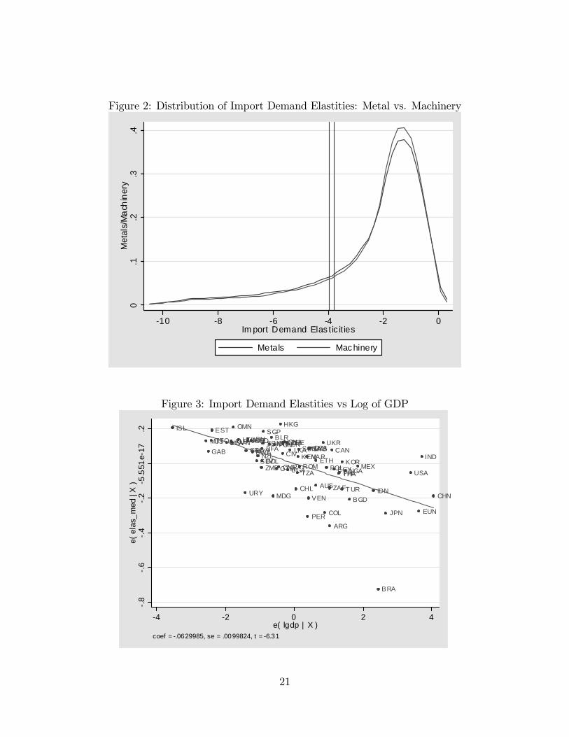
Figure 2: Distribution of Import Demand Elastities: Metal vs. Machinery
0
.1.2
.3.4
Met
als/
Ma
chin
ery
-10 -8 -6 -4 -2 0Im port Demand Elas t ic it ies
Metals Mac hinery
Figure 3: Import Demand Elastities vs Log of GDP
ISL
MUS
GAB
TTO
EST
LVAALBSVN
OMN
LTU
URY
CRI
JORLBNHND
RWAPRY
SLVNZL
ZMBBOL
BFASEN
SGP
NORBLR
MDG
T UN
GTMCMR
HKG
HUN
CIV
CZEGHACHE
UGA
LKA
CHL
TZA
KENSDN
ROM
MAR
PER
VEN
SAUMYSDZA
AUS
ETH
UKR
COL
POL
ZAF
ARG
CAN
EGYTHAPHL
T UR
KORNGA
BGD
MEX
IDN
BRA
JPN
USA
EUN
IND
CHN
-.8
-.6
-.4
-.2
-5.5
51e-
17.2
e( e
las_
med
| X
)
-4 -2 0 2 4e( lgdp | X )
coef = -.0629985, se = .0099824, t = -6.31
21

Figure 4: Import Demand Elastities vs Log of GDP per Capita
IND
CHNETHNGA
BGD
T ZAIDN
SDN
KEN
MDG
UGA
PHL
UKR
BFA
GHA
EGY
RWA
ZMB
BRA
CMR
LKACIV
MEXMARTHA
DZA
TUR
SEN
COL
ROM
HND
PER
BOLEUNZAF
POL
GTM
BLR
VEN
USA
ALB
MYST UN
ARG
SLV
PRY
JOR
KORSAU
CHLJPN
CZEHUN
LT ULBN
CAN
LVACRI
AUS
URY
OMN
EST
MUS
GAB
T TO
HKG
NZLSVN
SGPCHE
NORISL
-.6
-.4
-.2
-5.5
51e-
17.2
e( e
las_
med
| X
)
-4 -2 0 2 4e( lgdppc | X )
coef = .03168769, se = .01290625, t = 2.46
22

Figure 5: Estimated elasticities: sample moments
Country Simple Average
Standard Deviation
Median Import-weighted Average
Country Simple Average
Standard Deviation
Median Import-weighted Average
Country Simple Average
Standard Deviation
Median Import-weighted Average
ARE -3.84 7.51 -1.55 -1.59 FRA -4.18 7.93 -1.75 -2.31 MWI -2.52 4.44 -1.34 -1.39
ARG -6.31 11.57 -2.47 -3.41 GAB -4.02 7.5 -1.82 -1.8 MYS -3.19 7.02 -1.34 -1.36
ARM -3.01 4.88 -1.47 -1.34 GBR -4.02 7.77 -1.77 -2.08 NER -3.79 6.64 -1.74 -1.71
AUS -5.23 9.82 -2.06 -2.73 GEO -3.98 6.03 -1.98 -1.77 NGA -5.16 9.5 -1.99 -1.96
AUT -3.47 6.76 -1.49 -1.8 GHA -3.69 7.2 -1.56 -1.49 NIC -2.31 4.36 -1.29 -1.33
AZE -4.19 7.51 -1.66 -1.81 GIN -4.53 8.49 -1.88 -1.85 NLD -3.37 6.94 -1.44 -1.67
BDI -2.31 3.15 -1.33 -1.56 GMB -1.77 2.47 -1.17 -1.22 NOR -4.48 8.94 -1.72 -2.04
BEL -2.74 6 -1.29 -1.46 GRC -3.82 7.44 -1.75 -2.07 NZL -4.16 8.17 -1.72 -2.02
BEN -4.04 7.5 -1.68 -1.54 GTM -4.54 9.08 -1.81 -1.85 OMN -4.32 8.76 -1.48 -1.35
BFA -3.5 6.41 -1.59 -1.59 GUY -1.6 3.43 -1.09 -1.16 PAN -3.83 7.39 -1.57 -1.77
BGD -6.01 10.65 -2.23 -2.04 HKG -2.89 6.47 -1.21 -1.19 PER -5.21 9.46 -2.17 -2.38
BGR -3.32 6.41 -1.48 -1.63 HND -2.89 5.53 -1.39 -1.41 PHL -4.02 7.66 -1.7 -1.59
BLR -3.22 6.49 -1.33 -1.42 HRV -2.91 5.86 -1.4 -1.65 POL -3.45 7.18 -1.52 -1.83
BLZ -1.69 2.08 -1.2 -1.24 HUN -2.76 5.26 -1.37 -1.49 PRT -3.17 6.49 -1.51 -1.77
BOL -4.09 7.44 -1.83 -1.86 IDN -4.76 9.18 -1.75 -2.11 PRY -3.99 7.29 -1.67 -1.73
BRA -7.27 12.18 -2.82 -4.11 IND -7.71 12.81 -2.92 -3.67 ROM -3.27 6.07 -1.57 -1.76
BRB -2.65 5.58 -1.32 -1.52 IRL -3.44 7.08 -1.46 -1.6 RWA -3.82 6.35 -1.68 -1.97
CAF -2.72 3.5 -1.47 -1.61 IRN -5.28 10.13 -2.04 -1.98 SAU -4.53 8.54 -1.78 -1.97
CAN -4.47 8.8 -1.76 -2.02 ISL -3.9 7.87 -1.54 -1.79 SDN -5.92 10.69 -2.09 -1.86
CHE -3.97 8.55 -1.52 -1.89 ISR -2.11 1.65 -1.51 -1.46 SEN -3.52 6.18 -1.63 -1.55
CHL -4.15 8.35 -1.7 -1.99 ITA -4.33 7.83 -1.91 -2.38 SGP -2.49 5.75 -1.21 -1.2
CHN -5.04 9.3 -1.91 -2.43 JAM -3.27 6.78 -1.43 -1.41 SLV -4.19 8.39 -1.68 -1.81
CIV -5.3 9.28 -2.09 -1.87 JOR -3.23 6.65 -1.44 -1.4 SUR -1.24 0.76 -1.04 -1.06
CMR -5.65 9.59 -2.33 -2.2 JPN -9.15 14.7 -3.38 -4.14 SVK -2.69 5.14 -1.32 -1.46
COG -3.23 5.59 -1.5 -1.51 KEN -4.46 8.31 -1.79 -1.73 SVN -2.78 5.7 -1.29 -1.48
COL -5.01 9.11 -2.02 -2.49 KOR -4.41 8.17 -1.68 -2.05 SWE -4.09 8.37 -1.62 -1.95
COM -1.86 2.38 -1.23 -1.27 LBN -3.94 7.92 -1.57 -1.54 TGO -2.83 5.1 -1.46 -1.43
CRI -3.61 7.06 -1.55 -1.63 LKA -4.12 8.34 -1.54 -1.55 THA -4.09 8.78 -1.52 -1.7
CYP -3.19 6.29 -1.44 -1.54 LTU -3.3 6.78 -1.44 -1.52 TTO -3.36 7.42 -1.45 -1.57
CZE -2.65 5.27 -1.3 -1.47 LVA -3.05 6.63 -1.4 -1.54 TUN -3.39 7.14 -1.44 -1.5
DEU -4.17 7.82 -1.82 -2.2 MAR -4.24 8.33 -1.7 -1.87 TUR -4.4 8.34 -1.84 -2.3
DNK -3.95 8.2 -1.63 -1.93 MDG -3.77 6.7 -1.85 -2.28 TZA -4.72 8.91 -1.9 -2.03
DZA -4.75 8.41 -1.94 -1.95 MDV -1.54 2.17 -1.13 -1.18 UGA -5.17 9.32 -2 -2.14
EGY -5.15 9.48 -1.96 -2.05 MEX -4.02 7.93 -1.72 -2.05 UKR -4.64 8.86 -1.81 -1.7
ESP -4.02 7.61 -1.82 -2.33 MKD -2.79 5.32 -1.44 -1.56 URY -4.84 9.2 -1.96 -2.21
EST -2.22 4.51 -1.2 -1.27 MLI -4.17 7.88 -1.67 -1.48 USA -7.44 12.38 -2.8 -3.33
ETH -3.94 7.07 -1.69 -1.79 MLT -2.51 5.14 -1.29 -1.35 VEN -5.07 9.47 -2.08 -2.51
FIN -4.09 7.85 -1.71 -2.13 MNG -2.13 3.56 -1.22 -1.26 ZAF -4.85 9.38 -1.87 -2.37
MUS -2.85 5.91 -1.38 -1.43 ZMB -3.1 5.06 -1.56 -1.62
23