Estimating larval fish growth under size-dependent mortality: a numerical analysis of bias

Tian Tian, Øyvind Fiksen, and Arild Folkvord

Abstract: The early larval phase is characterized by high growth and mortality rates. Estimates of growth from bothpopulation (cross-sectional) and individual (longitudinal) data may be biased when mortality is size-dependent. Here,we use a simple individual-based model to assess the range of bias in estimates of growth under various size-dependentpatterns of growth and mortality rates. A series of simulations indicate that size distribution of individuals in the popu-lation may contribute significantly to bias in growth estimates, but that typical size-dependent growth patterns haveminor effects. Growth rate estimates from longitudinal data (otolith readings) are closer to true values than estimatesfrom cross-sectional data (population growth rates). The latter may produce bias in growth estimation of about0.03 day–1 (in instantaneous, specific growth rate) or >40% difference in some situations. Four potential patterns ofsize-dependent mortality are tested and analyzed for their impact on growth estimates. The bias is shown to yield largedifferences in estimated cohort survival rates. High autocorrelation and variance in growth rates tend to increase growthestimates and bias, as well as recruitment success. We also found that autocorrelated growth patterns, reflecting envi-ronmental variance structure, had strong impact on recruitment success of a cohort.

Résumé : Le début de la phase larvaire se caractérise par des taux élevés de croissance et de mortalité. L’estimationde la croissance à l’aide de données provenant de la population (transversales) et des individus (longitudinales) peutêtre faussée lorsque la mortalité est dépendante de la taille. Nous utilisons ici un modèle simple basé sur l’individuafin d’évaluer l’étendue de l’erreur dans les estimations de croissance sous divers patrons de taux de croissance et demortalité reliés à la taille. Une série de simulations indique que la distribution en taille des individus dans la popula-tion peut contribuer significativement à l’erreur des estimations de croissance, mais que les patrons typiques de crois-sance dépendant de la taille n’ont que des effets mineurs. Les estimations de la croissance à partir de donnéeslongitudinales (lectures d’otolithes) sont plus près des valeurs réelles que les estimations à partir de données transversa-les (taux de croissance de la population). Ces dernières peuvent générer une erreur dans l’estimation de la croissanced’environ 0,03 jour–1 (taux spécifique instantané de croissance) ou une différence de >40 % dans certains cas. Noustestons quatre patrons potentiels de mortalité taille dépendante et analysons leur impact sur les estimations de crois-sance. Nous montrons que cette erreur produit d’importantes différences dans les estimations de taux de survie de lacohorte. Une autocorrélation et une variance importantes des taux de croissance ont tendance à faire augmenter lesestimations de la croissance, l’erreur ainsi que le succès du recrutement. Nous observons également que les patrons decroissance autocorrélés, qui représentent la structure de la variance environnementale, ont un fort impact sur le succèsdu recrutement d’une cohorte.

[Traduit par la Rédaction] Tian et al. 562

Introduction

The early life history of fish is characterized by high ratesof mortality (Cushing 1975; Bailey and Houde 1989;Leggett and Deblois 1994). Survival of marine pelagic or-ganisms (e.g., eggs and larvae) change with size: larger indi-viduals typically have lower risk of mortality (Peterson andWroblewski 1984; McGurk 1986). The “growth–mortality”hypothesis argues that faster-growing and -developing larvaeare more likely to pass through each stage rapidly, therebylowering the cumulated mortality during early stages (Bailey

and Houde 1989). Many fish species have allometric, dome-shaped specific growth rates, increasing during early ontog-eny, leveling off, and eventually decreasing with size (Fondset al. 1992; Folkvord 2005). The interaction between size-dependent growth and mortality affects the size distributionof larval survivors (Huston et al. 1988) and necessitates adistinction between population growth rates and true meangrowth rates of individual fish (Ricker 1975), but it isknown that bias is introduced when using mean values ofpopulation data under high mortality rates (e.g., Otterå1992).

Can. J. Fish. Aquat. Sci. 64: 554–562 (2007) doi:10.1139/F07-031 © 2007 NRC Canada

554

Received 22 June 2006. Accepted 13 December 2006. Published on the NRC Research Press Web site at http://cjfas.nrc.ca on14 April 2007.J19381

T. Tian,1,2 Ø. Fiksen, and A. Folkvord. Department of Biology, University of Bergen, P.O. Box 7800, 5020 Bergen, Norway.

1Corresponding author (e-mail: tian.tian@gkss.de).2Present address: Institute for Coastal Research, GKSS Research Center, Max Planck Street 1, Building 11 (KOE), 21502Geesthacht, Germany.

One way to estimate growth is to group discrete popula-tion samples and compare mean size of surviving fish at suc-cessive ages. This is termed “cross-sectional” data analysisfor population growth rate. Such analysis assumes no size-biased sampling or mortality between sampling intervals(Ricker 1975). Alternatively, “longitudinal” data from otolithreadings use individual growth trajectories of sampled larvae(Chambers and Miller 1995). However, longitudinal growthestimates of survivors from the same cohort sampled at dif-ferent times will differ under significant size-dependent mor-tality as some size fractions are less likely to be included insubsequent samples. The classical example is when biasemerges as a result of size selection by a fishery (“Lee’sphenomenon”; Ricker 1975).

Given the absence of correction for size-dependent mor-tality in larval fish growth estimates, it is instructive to knowunder which conditions bias occurs. Both growth and mor-tality are highly nonlinear processes and the interactionsbetween them are far from trivial. Huston and DeAngelis(1987) listed four critical factors responsible for changes insize distributions as individuals develop: (i) the initial sizedistribution; (ii) the distribution of growth rates among theindividuals; (iii) the size and time dependence of the growthrate of each individual; and (iv) size-dependent mortality.Furthermore, short-term, small-scale environmental variabil-ity are expected to affect cohort survival rate (Letcher andRice 1997; Pitchford and Brindley 2001; Pitchford et al.2005), and thus the mean properties from population datamay not accurately predict development and survival of fishpopulations (Rice et al. 1993; Gallego et al. 1996; Pepin2004).

The many advantages of individual-based models (IBMs)in ecology have been discussed by various authors (Hustonet al. 1988; DeAngelis and Gross 1992; Grimm and Rails-back 2005). Here we use an IBM to trace growth and sur-vival of a larval cohort through early life stages undervarious scenarios of size-dependent growth and mortalityrates. Knowing the growth rates of survivors, we then esti-mate daily growth rates of the developing population withcross-sectional or longitudinal methods (Ricker 1975;Chambers and Miller 1995). The biases are obtained bycomparing average growth rates of individuals at successiveages with the average growth rates of final survivors. Thepotential magnitudes and patterns of bias are evaluated ac-cording to three patterns or mechanisms of size-dependentmortality rate: (i) decreasing with size (Peterson andWroblewski 1984; McGurk 1986); (ii) increasing with size(visual predation); and (iii) threshold size dependence inescape (e.g., gape-limited intracohort cannibalism). Two spe-cies with different allometric growth patterns (larval Atlanticcod (Gadus morhua) and Atlantic herring (Clupeaharengus)) are chosen as model organisms. Cod larvae havea dome-shaped growth potential with size (Otterlei et al.1999), whereas growth rate in larval herring is relatively in-dependent of size (Fiksen and Folkvord 1999). We also in-vestigate bias under variable and autocorrelated growthrates, which is anticipated for patchy environments, and howthis environmental structure affects cohort survival in themodel. In summary, we wish to determine (i) the magnitudeof bias induced by using mean values of population data;(ii) how potential bias of growth varies with larval size, ini-

tial size distribution, and the allometric patterns of growth-and size-dependent mortality regimes; and (iii) the effects ofenvironmental variability on larval survival and growth esti-mates.

Materials and methods

The individual-based model is initialized with a cohort of2-day-old yolk-sac larval cod. Population size declines dra-matically as the result of size-dependent mortality, thereforethe “super-individual” concept (Scheffer et al. 1995) is ap-plied (grouping together many individuals with identical at-tributes). We let 104 super-individuals represent the larvalcohort. Four attributes characterize each super-individuali over time: dry weight (DWi , mg), standard length(SLi , mm), probability of survival (Psi), and the number ofidentical individual survivors (Ni) represented by each super-individual. (Appendix A defines all symbols used for growthestimates in the IBM.) Age is implicit as only a single co-hort is traced. Simulations run until larvae reach an age of60 days posthatch (DPH) in time steps of 1 h. Data of allsuper-individuals are stored once each day and comparedwith population assessments.

Larval growth modelsDaily growth (SGR, %·day–1) of larval Norwegian coastal

cod (Gadus morhua) under optimal conditions in the lab is afunction of dry body mass (DW, mg) and water temperature(T, °C) (Otterlei et al. 1999; Folkvord 2005):

(1) SGR DW 1.20 1.80 0.078 DW( , ) (ln )T T T= + −− +0.0946 DW 0.0105 DW2 3T T(ln ) (ln )

Here, we keep the temperature fixed at 6 °C, and then thistranslates to a specific instantaneous growth rate gc,i(DWi)of larval cod i with body mass DWi:

(2) g i ii

c DWSGR 6,DW

1001, ( ) ln

( )= +

For herring-like species, instantaneous growth rate gh,i isindependent of size, and because temperature is fixed at6 °C, growth is a constant (Fiksen and Folkvord 1999):

(3) gh i, = − + × =0.024 0.012 6 0.048

Environmental stochasticity in growth ~,g ic (DWi, t) was mod-

eled as an autocorrelated process (Ripa and Lundberg 1996):

(4)~ ( , ) ( ) ( ) ( )

( ) (

, , ,g t g e t g

e t e t

i i i i i i i

i i

c c cDW DW DW= +

= ⋅ −α 1 0,1) 1 2) (+ ⋅ ⋅ −σ αn

where t is time in hours (ei was reset once each day), n(0,1) isa random number drawn from a standard normal distribution,α is the autocorrelation coefficient (0 ≤ α ≤ 1), and σ is stan-dard deviation (variance = σ2). The growth rate ~

,g ic (DWi ,t)was not allowed to exceed 50% of the expected growth rateat any age, or to be less than 0. Equation 4 is practical ingenerating variability into individual growth trajectories,with no (α = 0) or high autocorrelation (α approach 1) intime. For larval fish, this mimics a situation where growthrates of individuals are influenced by a patchy environmentresulting from patchy prey, temperature, or other environ-

© 2007 NRC Canada

Tian et al. 555

mental factors affecting growth. Low autocorrelation wouldsimulate a fine-grained environment in which the likelihoodof switching between good and bad environments on shorttime scales is high. High autocorrelation mimics morecoarse-grained environments, so that a larva in a good orbad environment is likely to remain in this condition forsome time. The structure of the environment may have im-plications for emerging size distributions of larval cohortsthrough distribution of growth rates among individuals and,consequently, their survival probabilities and bias of growthestimates.

Larval mortality ratesMortality or predation rates of larval fish are typically

highly size-dependent. If invertebrate predators are the dom-inating predators, risk of predation tends to decrease withsize, but if visual predators are important, risk of predationmay increase with size (Bailey and Houde 1989). Here, wehave applied four basic models of changes in mortality rateswith size, two empirical models in which mortality dropswith size, one in which risk increases, and one that chops offthe smaller fraction of the cohort every week.

The daily natural mortality rates MP (day–1) of pelagic or-ganisms are observed to be dependent on body mass (Peter-son and Wroblewski 1984):

(5) MP3 3 0.255.3 10 10 DW= × − − −( )

McGurk (1986) found mortality rates MM (day–1) of fisheggs and larvae to be even more size-dependent:

(6) MM4 3 0.852.2 10 10 DW= × − − −( )

Predation rate from fish Mf (day–1) is assumed to be an in-creasing function of larval SL if other factors such as light,larval behavior, or depth of occurrence are held constant(Fiksen et al. 2002):

(7) Mf4 25.5 10 SL= × −

In some situations, such as during intensive cannibalism orpredation from an abundant gape-limited predator, all larvae be-low a given size may be removed from the population. In somesituations, this could generate strong bias in growth estimates(Folkvord 1997). We remove larvae shorter than the averagebody length from the population at weekly intervals and refer tothis mortality as Mc. SL (mm) as a function of body mass isSL = exp[2.296 + 0.277(lnDW) – 0.005128(lnDW)2] for lar-val cod (Folkvord 2005) and SL = 4.76[ln(103 DW) – 2.9] forlarval herring (Fiksen and Folkvord 1999).

Given a size-dependent mortality rate M[DWi(t)] (i.e., MP,MM, Mf , or Mc), the probability Psi(t) of surviving one day(∆t) for each super-individual i depends on body mass andsize dependency in mortality:

(8) Ps tiM t ti( ) [ ( )]= −e DW ∆

The number of individual survivors represented by eachsuper-individual Ni will decrease with Psi(t), such that eachsuper-individual i represents fewer individuals over time.Super-individuals (104 individuals) are followed (60 days),each initially representing 106 (cod-like growth pattern) or108 individuals (herring-like growth pattern).

Estimating population growth and defining biasPopulation growth rate gcs(t) at time t (= age of cohort)

from cross-sectional methods is estimated by using meanweight of individual larvae at successive days (Folkvord1997):

(9) g tt t

tcs

DW DW 1( )

ln ( ) ln ( )= − −∆

where DW( )t and DW 1( )t − are the mean body sizes (mg dryweight) of all individuals at days t and t – 1 (time interval∆t = 1 day) from

(10) DW

DW 1

( )

( ) ( ) ( )

(

t

t N t Ps t

N t

ii

i i

ii

=⋅ − ⋅

−

=

=

∑

∑1

10000

1

10000

1) ( )⋅Ps ti

The total abundance N tii=∑

1

10000

( ) at t differs from that at t – 1 as

some individuals die during this time interval as a result ofsize-dependent mortality. However, estimates of true meangrowth rates (as defined by us) require initial and final meanweights from the same individuals (Fig. 1a). To follow thegrowth rates of survivors only, we first ran the model for-ward for 60 days, stored the size development of the finalsurviving larvae, and calculated what we defined as truedaily mean growth rate gTMG:

(11) g t

N g t

N

ii

i i

ii

TMG

60 DW

60

( )

( ) ( , )

( )

=⋅

=

=

∑

∑1

10000

1

10000

With longitudinal data, the use of otoliths can yield infor-mation about individual growth trajectories that reflect truegrowth rates of survivors from samples at time t + 1:

(12) g t

N t g t

N t

ii

i i

ii

lon

c1 DW

( )

( ) ( , )

(

,

=+ ⋅

+

=

=

∑

∑1

10000

1

10000

1)

However, a sample of individuals from any time (or co-hort age) t (2 < t < 60 DPH in the model) will give differentgrowth histories compared with the final cohort under size-dependent mortality. This is because the final sample willconsist of a size-biased subsample of all previous samples.We define bias inherent in longitudinal estimates as the dif-ference in growth at age between a sample of survivors at 60DPH and any sample from t < 60 DPH. Technically, the biasfrom cross-sectional εcs or longitudinal εlon data (Fig. 1b) isgiven by

(13) ε εcs cs TMG lon lon TMGand= − = −g g g g

Note that there will be no bias in any estimate if mortality isnot dependent on larval size (constant mortality rate).

© 2007 NRC Canada

556 Can. J. Fish. Aquat. Sci. Vol. 64, 2007

Overview of simulationsUnless specified otherwise, the initial dry weight of each

super-individual is a normal deviate from a size distributionwith mean dry weight (± standard deviation, SD) of 0.034 ±0.006 mg (restricted downwards to 0.02 mg) as in the rear-ing experiment of Otterlei et al. (1999). As a standard, thegrowth pattern is dome-shaped with size (eq. 1), temperatureis fixed at 6 ºC, the mortality rate MM from McGurk (1986)is used, and bias is given from cross-sectional assessment,with sampling intervals of 1 day.

We investigated the following potential candidates for biasin growth estimates.

Experiment 1: initial size distributionWe simulated growth estimates using initial body sizes

from a normal (0.034 ± 0.006 mg) and a uniform (0.034 ±0.01 mg) distribution with a fixed coefficient of variation

(CV) of 17%. Cohort variance in weight distribution devel-ops naturally from growth and mortality processes.

Experiment 2: initial body size and size variabilityWe initiated 10 cohorts with increasing mean weights

(i.e., 0.034, 0.05, 0.1, 0.3, 0.5, 1.0, 3.0, 5.0, 10.0, and30.0 mg). The cohorts were given CVs either fixed at 17%(populations were regenerated at each size category) oremerging naturally from a developing cohort. The estimatedemergent CVs for each cohort in this case were 17%, 24%,32%, 39%, 41%, 41%, 38%, 35%, 31%, and 24%, respec-tively. In this case, bias is obtained by comparing the popu-lation growth rate at 1-week intervals, and each cohort isassessed only once to mimic discrete sampling in the field.

Experiment 3: growth patternWe simulated one cohort with dome-shaped growth rates

(gc, eq. 2) and one with constant specific growth rates (gh,eq. 3) starting from the same initial population.

Experiment 4: size-dependent mortality rateEach mortality model (MM, MP, Mf , and Mc) was assessed

for effects on bias.

Experiment 5: demographic and environmentalstochasticity

The stochasticity parameters α and σ (eq. 4) were variedand both bias and recruitment success were compared withdeterministic simulations.

Results

Experiment 1: initial size distributionBias decreases near exponentially with age for both nor-

mal and uniform initial size distributions (Fig. 2a). A uni-formly distributed larval cohort is more biased initially, butthe normally distributed cohort becomes more biased afterabout 1 week. The maximal bias of 0.027 day–1 is about40% of the true mean growth rate of 0.06 day–1, but the biasdecreases to less than 0.01 day–1 within 10 days.

Experiment 2: initial body size and size variabilityFor initial populations of increasing average weight but

constant CV of 17%, bias peaks at 0.024 day–1 and de-creases exponentially with weight (Fig. 2b). For initial popu-lations with varying CVs, bias peaks at around 0.1 mg(0.03 day–1). The size variation increases from 17% of thefirst initial population (smallest average size) to 32% of thethird initial population owing to the dome-shaped growthpattern. The CV peaks (41%) at 0.5~1.0 mg, but the bias ofgrowth estimates declines before this because mortality ratedrops with weight and supersedes the effect of increasingvariance. The mean body size of the initial population hassome influence owing to the size-specific mortality functionMM, but the main factor generating biased estimates isweight variability of initial population (i.e., CV).

Experiment 3: growth patternWhen applying a size-independent growth rate (Fig. 2c),

the constant CV of the size distribution will be preserved (asin experiment 2) and growth estimates are biased only by

© 2007 NRC Canada

Tian et al. 557

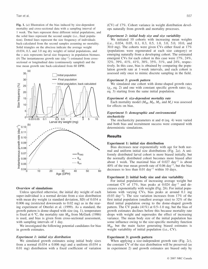
Fig. 1. (a) Illustration of the bias induced by size-dependentmortality and cross-sectional data with a sampling interval of1 week. The bars represent three different initial populations, andthe solid lines represent the second sample (i.e., final popula-tion). Dotted lines represent the size frequency of individualsback-calculated from the second samples assuming no mortality.Solid triangles on the abscissa indicate the average weight(0.034, 0.3, and 3.0 mg dry weight) of initial populations, andthe y axis represents larval size frequency in population biomass.(b) The instantaneous growth rate (day–1) estimated from cross-sectional or longitudinal data (continuously sampled) and thetrue mean growth rate back-calculated from 60 DPH.

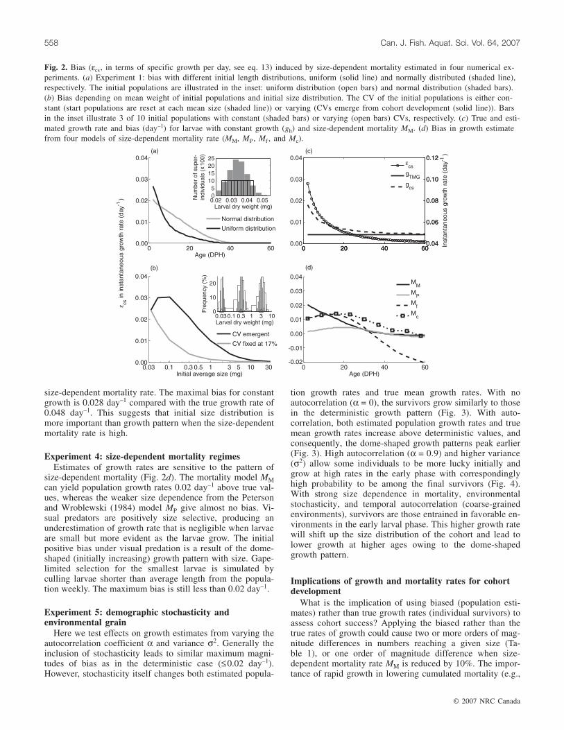
size-dependent mortality rate. The maximal bias for constantgrowth is 0.028 day–1 compared with the true growth rate of0.048 day–1. This suggests that initial size distribution ismore important than growth pattern when the size-dependentmortality rate is high.

Experiment 4: size-dependent mortality regimesEstimates of growth rates are sensitive to the pattern of

size-dependent mortality (Fig. 2d). The mortality model MMcan yield population growth rates 0.02 day–1 above true val-ues, whereas the weaker size dependence from the Petersonand Wroblewski (1984) model MP give almost no bias. Vi-sual predators are positively size selective, producing anunderestimation of growth rate that is negligible when larvaeare small but more evident as the larvae grow. The initialpositive bias under visual predation is a result of the dome-shaped (initially increasing) growth pattern with size. Gape-limited selection for the smallest larvae is simulated byculling larvae shorter than average length from the popula-tion weekly. The maximum bias is still less than 0.02 day–1.

Experiment 5: demographic stochasticity andenvironmental grain

Here we test effects on growth estimates from varying theautocorrelation coefficient α and variance σ2. Generally theinclusion of stochasticity leads to similar maximum magni-tudes of bias as in the deterministic case (≤0.02 day–1).However, stochasticity itself changes both estimated popula-

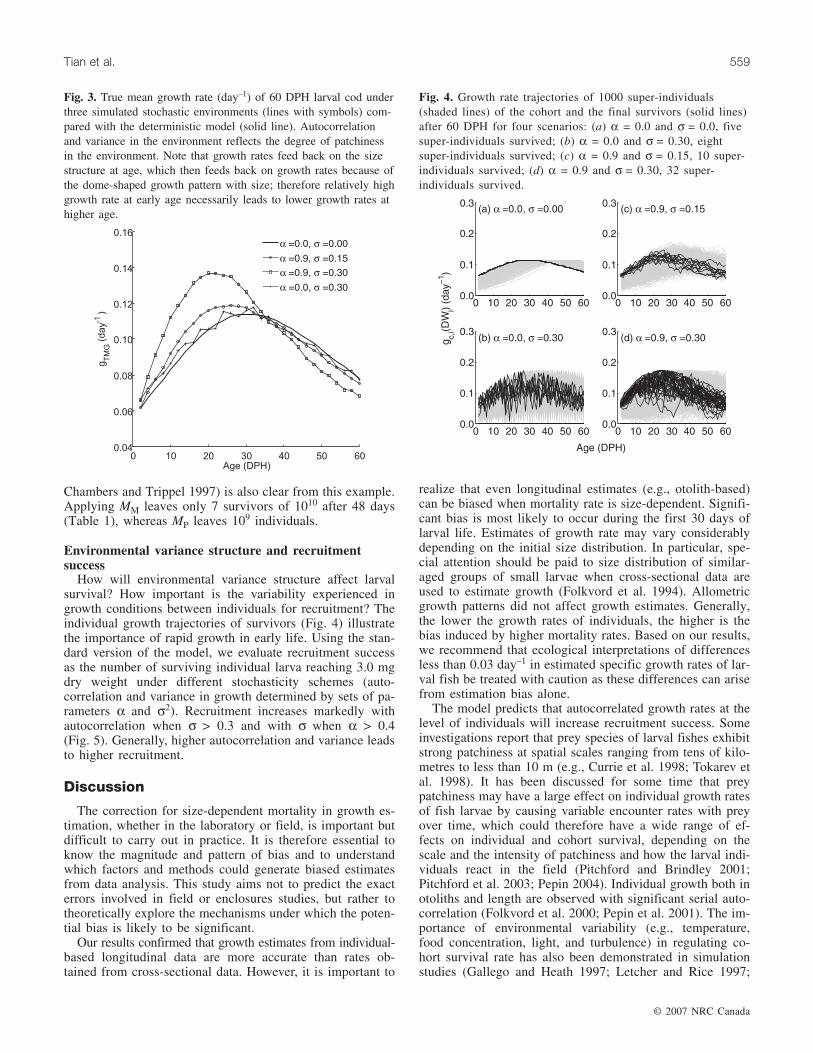
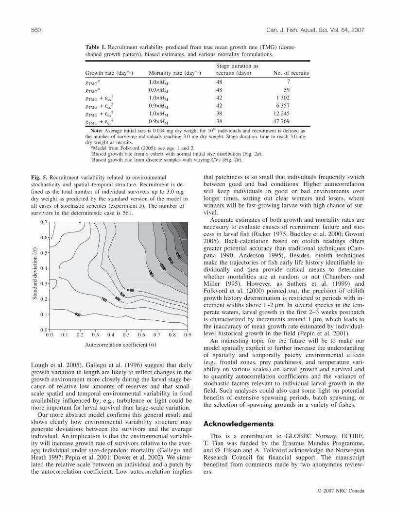
tion growth rates and true mean growth rates. With noautocorrelation (α = 0), the survivors grow similarly to thosein the deterministic growth pattern (Fig. 3). With auto-correlation, both estimated population growth rates and truemean growth rates increase above deterministic values, andconsequently, the dome-shaped growth patterns peak earlier(Fig. 3). High autocorrelation (α = 0.9) and higher variance(σ2) allow some individuals to be more lucky initially andgrow at high rates in the early phase with correspondinglyhigh probability to be among the final survivors (Fig. 4).With strong size dependence in mortality, environmentalstochasticity, and temporal autocorrelation (coarse-grainedenvironments), survivors are those entrained in favorable en-vironments in the early larval phase. This higher growth ratewill shift up the size distribution of the cohort and lead tolower growth at higher ages owing to the dome-shapedgrowth pattern.

Implications of growth and mortality rates for cohortdevelopment

What is the implication of using biased (population esti-mates) rather than true growth rates (individual survivors) toassess cohort success? Applying the biased rather than thetrue rates of growth could cause two or more orders of mag-nitude differences in numbers reaching a given size (Ta-ble 1), or one order of magnitude difference when size-dependent mortality rate MM is reduced by 10%. The impor-tance of rapid growth in lowering cumulated mortality (e.g.,

© 2007 NRC Canada

558 Can. J. Fish. Aquat. Sci. Vol. 64, 2007

Fig. 2. Bias (εcs, in terms of specific growth per day, see eq. 13) induced by size-dependent mortality estimated in four numerical ex-periments. (a) Experiment 1: bias with different initial length distributions, uniform (solid line) and normally distributed (shaded line),respectively. The initial populations are illustrated in the inset: uniform distribution (open bars) and normal distribution (shaded bars).(b) Bias depending on mean weight of initial populations and initial size distribution. The CV of the initial populations is either con-stant (start populations are reset at each mean size (shaded line)) or varying (CVs emerge from cohort development (solid line)). Barsin the inset illustrate 3 of 10 initial populations with constant (shaded bars) or varying (open bars) CVs, respectively. (c) True and esti-mated growth rate and bias (day–1) for larvae with constant growth (gh) and size-dependent mortality MM. (d) Bias in growth estimatefrom four models of size-dependent mortality rate (MM, MP , Mf , and Mc).

Chambers and Trippel 1997) is also clear from this example.Applying MM leaves only 7 survivors of 1010 after 48 days(Table 1), whereas MP leaves 109 individuals.

Environmental variance structure and recruitmentsuccess

How will environmental variance structure affect larvalsurvival? How important is the variability experienced ingrowth conditions between individuals for recruitment? Theindividual growth trajectories of survivors (Fig. 4) illustratethe importance of rapid growth in early life. Using the stan-dard version of the model, we evaluate recruitment successas the number of surviving individual larva reaching 3.0 mgdry weight under different stochasticity schemes (auto-correlation and variance in growth determined by sets of pa-rameters α and σ2). Recruitment increases markedly withautocorrelation when σ > 0.3 and with σ when α > 0.4(Fig. 5). Generally, higher autocorrelation and variance leadsto higher recruitment.

Discussion

The correction for size-dependent mortality in growth es-timation, whether in the laboratory or field, is important butdifficult to carry out in practice. It is therefore essential toknow the magnitude and pattern of bias and to understandwhich factors and methods could generate biased estimatesfrom data analysis. This study aims not to predict the exacterrors involved in field or enclosures studies, but rather totheoretically explore the mechanisms under which the poten-tial bias is likely to be significant.

Our results confirmed that growth estimates from individual-based longitudinal data are more accurate than rates ob-tained from cross-sectional data. However, it is important to

realize that even longitudinal estimates (e.g., otolith-based)can be biased when mortality rate is size-dependent. Signifi-cant bias is most likely to occur during the first 30 days oflarval life. Estimates of growth rate may vary considerablydepending on the initial size distribution. In particular, spe-cial attention should be paid to size distribution of similar-aged groups of small larvae when cross-sectional data areused to estimate growth (Folkvord et al. 1994). Allometricgrowth patterns did not affect growth estimates. Generally,the lower the growth rates of individuals, the higher is thebias induced by higher mortality rates. Based on our results,we recommend that ecological interpretations of differencesless than 0.03 day–1 in estimated specific growth rates of lar-val fish be treated with caution as these differences can arisefrom estimation bias alone.

The model predicts that autocorrelated growth rates at thelevel of individuals will increase recruitment success. Someinvestigations report that prey species of larval fishes exhibitstrong patchiness at spatial scales ranging from tens of kilo-metres to less than 10 m (e.g., Currie et al. 1998; Tokarev etal. 1998). It has been discussed for some time that preypatchiness may have a large effect on individual growth ratesof fish larvae by causing variable encounter rates with preyover time, which could therefore have a wide range of ef-fects on individual and cohort survival, depending on thescale and the intensity of patchiness and how the larval indi-viduals react in the field (Pitchford and Brindley 2001;Pitchford et al. 2003; Pepin 2004). Individual growth both inotoliths and length are observed with significant serial auto-correlation (Folkvord et al. 2000; Pepin et al. 2001). The im-portance of environmental variability (e.g., temperature,food concentration, light, and turbulence) in regulating co-hort survival rate has also been demonstrated in simulationstudies (Gallego and Heath 1997; Letcher and Rice 1997;

© 2007 NRC Canada

Tian et al. 559

Fig. 3. True mean growth rate (day–1) of 60 DPH larval cod underthree simulated stochastic environments (lines with symbols) com-pared with the deterministic model (solid line). Autocorrelationand variance in the environment reflects the degree of patchinessin the environment. Note that growth rates feed back on the sizestructure at age, which then feeds back on growth rates because ofthe dome-shaped growth pattern with size; therefore relatively highgrowth rate at early age necessarily leads to lower growth rates athigher age.

Fig. 4. Growth rate trajectories of 1000 super-individuals(shaded lines) of the cohort and the final survivors (solid lines)after 60 DPH for four scenarios: (a) α = 0.0 and σ = 0.0, fivesuper-individuals survived; (b) α = 0.0 and σ = 0.30, eightsuper-individuals survived; (c) α = 0.9 and σ = 0.15, 10 super-individuals survived; (d) α = 0.9 and σ = 0.30, 32 super-individuals survived.

Lough et al. 2005). Gallego et al. (1996) suggest that dailygrowth variation in length are likely to reflect changes in thegrowth environment more closely during the larval stage be-cause of relative low amounts of reserves and that small-scale spatial and temporal environmental variability in foodavailability influenced by, e.g., turbulence or light could bemore important for larval survival than large-scale variation.

Our more abstract model confirms this general result andshows clearly how environmental variability structure maygenerate deviations between the survivors and the averageindividual. An implication is that the environmental variabil-ity will increase growth rate of survivors relative to the aver-age individual under size-dependent mortality (Gallego andHeath 1997; Pepin et al. 2001; Dower et al. 2002). We simu-lated the relative scale between an individual and a patch bythe autocorrelation coefficient. Low autocorrelation implies

that patchiness is so small that individuals frequently switchbetween good and bad conditions. Higher autocorrelationwill keep individuals in good or bad environments overlonger times, sorting out clear winners and losers, wherewinners will be fast-growing larvae with high chance of sur-vival.

Accurate estimates of both growth and mortality rates arenecessary to evaluate causes of recruitment failure and suc-cess in larval fish (Ricker 1975; Buckley et al. 2000; Govoni2005). Back-calculation based on otolith readings offersgreater potential accuracy than traditional techniques (Cam-pana 1990; Anderson 1995). Besides, otolith techniquesmake the trajectories of fish early life history identifiable in-dividually and then provide critical means to determinewhether mortalities are at random or not (Chambers andMiller 1995). However, as Suthers et al. (1999) andFolkvord et al. (2000) pointed out, the precision of otolithgrowth history determination is restricted to periods with in-crement widths above 1~2 µm. In several species in the tem-perate waters, larval growth in the first 2~3 weeks posthatchis characterized by increments around 1 µm, which leads tothe inaccuracy of mean growth rate estimated by individual-level historical growth in the field (Pepin et al. 2001).

An interesting topic for the future will be to make ourmodel spatially explicit to further increase the understandingof spatially and temporally patchy environmental effects(e.g., frontal zones, prey patchiness, and temperature vari-ability on various scales) on larval growth and survival andto quantify autocorrelation coefficients and the variance ofstochastic factors relevant to individual larval growth in thefield. Such analyses could also cast some light on potentialbenefits of extensive spawning periods, batch spawning, orthe selection of spawning grounds in a variety of fishes.

Acknowledgements

This is a contribution to GLOBEC Norway, ECOBE.T. Tian was funded by the Erasmus Mundus Programme,and Ø. Fiksen and A. Folkvord acknowledge the NorwegianResearch Council for financial support. The manuscriptbenefited from comments made by two anonymous review-ers.

© 2007 NRC Canada

560 Can. J. Fish. Aquat. Sci. Vol. 64, 2007

Growth rate (day–1) Mortality rate (day–1)Stage duration asrecruits (days) No. of recruits

gTMG* 1.0×MM 48 7

gTMG* 0.9×MM 48 59gTMG + εcs

† 1.0×MM 42 1 302gTMG + εcs

† 0.9×MM 42 6 357gTMG + εcs

‡ 1.0×MM 38 12 245gTMG + εcs

‡ 0.9×MM 38 47 769

Note: Average initial size is 0.034 mg dry weight for 1010 individuals and recruitment is defined asthe number of surviving individuals reaching 3.0 mg dry weight. Stage duration: time to reach 3.0 mgdry weight as recruits.

*Model from Folkvord (2005); see eqs. 1 and 2.†Biased growth rate from a cohort with normal initial size distribution (Fig. 2a).‡Biased growth rate from discrete samples with varying CVs (Fig. 2b).

Table 1. Recruitment variability predicted from true mean growth rate (TMG) (dome-shaped growth pattern), biased estimates, and various mortality formulations.

Fig. 5. Recruitment variability related to environmentalstochasticity and spatial–temporal structure. Recruitment is de-fined as the total number of individual survivors up to 3.0 mgdry weight as predicted by the standard version of the model inall cases of stochastic schemes (experiment 5). The number ofsurvivors in the deterministic case is 561.

References

Anderson, C.S. 1995. Calculating size-dependent relative survivalfrom samples taken before and after selection. In Recent devel-opments in fish otolith research. Edited by D.H. Secor, J.M.Dean, and S.E. Campana. University of South Carolina Press,Columbia, S.C. pp. 455–466.

Bailey, K.M., and Houde, E.D. 1989. Predation on eggs and larvaeof marine fishes and the recruitment problem. Adv. Mar. Biol.25: 1–83.

Buckley, L.J., Lough, R.G., Peck, M.A., and Werner, F.E. 2000.Comment: larval Atlantic cod and haddock growth models, me-tabolism, ingestion, and temperature effects. Can. J. Fish. Aquat.Sci. 57: 1957–1960.

Campana, S.E. 1990. How reliable are growth back-calculationsbased on otoliths. Can. J. Fish. Aquat. Sci. 47: 2219–2227.

Chambers, R.C., and Miller, T.J. 1995. Evaluating fish growth bymeans of otolith increment analysis: special properties ofindividual-level longitudinal data. In Recent developments infish otolith research. Edited by D.H. Secor, J.M. Dean, and S.E.Campana. University of South Carolina Press, Columbia, S.C.pp. 155–175.

Chambers, R.C., and Trippel, E.A. 1997. Early life history and re-cruitment in fish populations. Chapman and Hall Ltd., London,UK.

Currie, W.J.S., Claereboudt, M.R., and Roff, J.C. 1998. Gaps andpatches in the ocean: a one-dimensional analysis of planktonicdistributions. Mar. Ecol. Prog. Ser. 171: 15–21.

Cushing, D.H. 1975. Marine ecology and fisheries. Cambridge Uni-versity Press, Cambridge, UK.

DeAngelis, D.L., and Gross, L.J. 1992. Individual based modelsand approaches in ecology: concepts and models. Routledge,Chapman and Hall, New York.

Dower, J.F., Pepin, P., and Leggett, W.C. 2002. Using patch studiesto link mesoscale patterns of feeding and growth in larval fish toenvironmental variability. Fish. Oceanogr. 11: 219–232.

Fiksen, Ø., and Folkvord, A. 1999. Modelling growth and inges-tion processes in herring Clupea harengus larvae. Mar. Ecol.Prog. Ser. 184: 273–289.

Fiksen, Ø., Aksnes, D.L., Flyum, M.H., and Giske, J. 2002. The in-fluence of turbidity on growth and survival of fish larvae: a nu-merical analysis. Hydrobiologia, 484: 49–59.

Folkvord, A. 1997. Ontogeny of cannibalism in larval and juvenilefish with special emphasis on Atlantic cod, Gadus morhua L. InEarly life history and recruitment in fish populations. Edited byR.C. Chambers and E.A. Trippel. Chapman and Hall Ltd., Lon-don, UK. pp. 251–278.

Folkvord, A. 2005. Comparison of size-at-age of larval Atlanticcod (Gadus morhua) from different populations based on size-and temperature-dependent growth models. Can. J. Fish. Aquat.Sci. 62: 1037–1052.

Folkvord, A., Øiestad, V., and Kvenseth, P.G. 1994. Growth pat-terns of three cohorts of Atlantic cod larvae (Gadus morhua L.)studied in a macrocosm. ICES J. Mar. Sci. 51: 325–336.

Folkvord, A., Blom, G., Johannessen, A., and Moksness, E. 2000.Growth-dependent age estimation in herring (Clupea harengus L.)larvae. Fish. Res. 46: 91–103.

Fonds, M., Cronie, R., Vethaak, A.D., and Van der Puyl, P. 1992. Me-tabolism, food consumption and growth of plaice (Pleuronectesplatessa) and flounder (Platichthys flesus) in relation to fish sizeand temperature. Neth. J. Sea Res. 29: 127–143.

Gallego, A., and Heath, M. 1997. The effect of growth-dependentmortality, external environment and internal dynamics on larval

fish otolith growth: an individual-based modelling approach. J.Fish Biol. 51(Suppl. A): 121–134.

Gallego, A., Heath, M.R., McKenzie, E., and Cargill, L.H. 1996.Environmentally induced short-term variability in the growthrates of larval herring. Mar. Ecol. Prog. Ser. 137: 11–23.

Govoni, J.J. 2005. Fisheries oceanography and the ecology of earlylife histories of fishes: a perspective over fifty years. Sci. Mar.69: 125–137.

Grimm, V., and Railsback, S.F. 2005. Individual-based modelingand ecology. Princeton Univeristy Press, Princeton, N.J.

Huston, M.A., and DeAngelis, D.L. 1987. Size bimodality in mono-specific populations: a critical review of potential mechanisms.Am. Nat. 129: 678–707.

Huston, M.A., DeAngelis, D.L., and Post, W. 1988. New computermodels unify ecological theory. Bioscience, 38: 682–691.

Leggett, W.C., and Deblois, E. 1994. Recruitment in marinefishes — is it regulated by starvation and predation in the eggand larval stages. Neth. J. Sea Res. 32: 119–134.

Letcher, B.H., and Rice, J.A. 1997. Prey patchiness and larval fishgrowth and survival: inferences from an individual-based model.Ecol. Model. 95: 29–43.

Lough, R.G., Buckley, L.J., Werner, F.E., Quinlan, J.A., and Ed-wards, K.P. 2005. A general biophysical model of larval cod(Gadus morhua) growth applied to populations on GeorgesBank. Fish. Oceanogr. 14: 241–262.

McGurk, M.D. 1986. Natural mortality of marine pelagic fish eggsand larvae: role of spatial patchiness. Mar. Ecol. Prog. Ser. 34:227–242.

Otterlei, E., Nyhammer, G., Folkvord, A., and Stefansson, S.O. 1999.Temperature- and size-dependent growth of larval and early juve-nile Atlantic cod (Gadus morhua): a comparative study of Norwe-gian coastal cod and northeast Arctic cod. Can. J. Fish. Aquat. Sci.56: 2099–2111.

Otterå, H. 1992. Bias in calculating growth rates in cod (Gadusmorhua L.) due to size selective growth and mortality. J. FishBiol. 40: 465–467.

Pepin, P. 2004. Early life history studies of prey–predator interac-tions: quantifying the stochastic individual responses to environ-mental variability. Can. J. Fish. Aquat. Sci. 61: 659–671.

Pepin, P., Dower, J.F., and Benoet, H.P. 2001. The role of measure-ment error on the interpretation of otolith increment width in thestudy of growth in larval fish. Can. J. Fish. Aquat. Sci. 58:2204–2212.

Peterson, I., and Wroblewski, J.S. 1984. Mortality rate of fishes inthe pelagic ecosystem. Can. J. Fish. Aquat. Sci. 41: 1117–1120.

Pitchford, J.W., and Brindley, J. 2001. Prey patchiness, predatorsurvival and fish recruitment. Bull. Math. Biol. 63: 527–546.

Pitchford, J.W., James, A., and Brindley, J. 2003. Optimal foragingin patchy turbulent environments. Mar. Ecol. Prog. Ser. 256: 99–110.

Pitchford, J.W., James, A., and Brindley, J. 2005. Quantifying theeffects of individual and environmental variability in fish re-cruitment. Fish. Oceanogr. 14: 156–160.

Rice, J.A., Miller, T.J., Rose, K.A. Crowder, L.B., Marschall, E.A.,Trebitz, A.S., and DeAngelis, D.L. 1993. Growth rate variation andlarval survival: inferences from an individual-based size-dependentpredation model. Can. J. Fish. Aquat. Sci. 50: 133–142.

Ricker, W.E. 1975. Computation and interpretation of biologicalstatistics of fish populations. Bull. Fish. Res. Board Can.No. 191.

Ripa, J., and Lundberg, P. 1996. Noise colour and the risk of popu-lation extinctions. Proc. R. Soc. Lond. B, 263: 1751–1753.

© 2007 NRC Canada

Tian et al. 561

Scheffer, M., Baveco, J.M., Deangelis, D.L., Rose, K.A., and Vannes,E.H. 1995. Super-individuals: a simple solution for modeling largepopulations on an individual basis. Ecol. Model. 80: 161–170.

Suthers, I.M., van der Meeren, T., and Jorstad, K.E. 1999. Growthhistories derived from otolith microstructure of three Norwegian

cod stocks co-reared in mesocosms: effect of initial size andprey size changes. ICES J. Mar. Sci. 56: 658–672.

Tokarev, Y.N., Williams, R., and Piontkovski, S.A. 1998. Small-scale plankton patchiness in the Black Sea euphotic layer. Hydro-biologia, 376: 363–367.

Appendix A

© 2007 NRC Canada

562 Can. J. Fish. Aquat. Sci. Vol. 64, 2007

Symbols Value and unit Description

DWi mg dry weight Dry weightSLi mm Standard lengthPsi — Probability of survivalNi Individuals The number of identical individual survivors represented by each super-individual. Initially 106

and 108 for cod- or herring-like speciesSGRi %·day–1 Size-specific growth rate of larval Norwegian coastal cod (Gadus morhua)gi (gc,i or gh,i) day–1 Instantaneous growth rate for cod- or herring-like species~

,gc i day–1 Instantaneous growth rate with environmental stochasticity for cod-like speciesei Error termα [0, 1] Autocorrelation coefficientσ [0, 0.7] Standard deviationMP(DWi) day–1 Mortality rate dependent on body mass (Peterson and Wroblewski 1984)MM(DWi) day–1 Mortality rate dependent on body mass (McGurk 1986)Mf (SLi) day–1 Predation rate increasing with standard lengthMc(SLi) week–1 Cannibalism predation rate dependent on relative standard length among the cohortgcs day–1 Instantaneous population growth rate from cross-sectional dataglon day–1 Instantaneous population growth rate from longitudinal datagTMG day–1 True mean growth rate of 60 DPH larvaeDW mg dry weight Mean body mass of a cohortεcs day–1 Bias from cross-sectional dataε lon day–1 Bias from longitudinal data

Table A1. Symbols used for growth estimates in the individual-based model.