ESTIMATING MARGINAL UTILITIES WITHOUT AGGREGATION · ESTIMATING MARGINAL UTILITIES WITHOUT AGGREGATION ETHAN LIGON Contents 1. Introduction 1 2. A Wrong urnT 2 3. An Alternative Approach

ESTIMATING MARGINAL UTILITIES WITHOUT

AGGREGATION

ETHAN LIGON

Contents

1. Introduction 12. A Wrong Turn 23. An Alternative Approach 64. Model of Household Behavior 85. Choosing Subsets of Goods and Services with which to

Estimate Marginal Utilities 106. The Variable Elasticity System of Demand 127. Estimation 148. Conclusion 199. References 20

20Appendix A. Application in Uganda 22

1. Introduction

The models economists use to describe dynamic consumer behav-ior almost invariably boil down to a description of how consumers'marginal utilities evolve over time. A central example involves thecanonical Euler equation, which describes how consumers smooth con-sumption over time when they have access to credit markets (Bewley,1977; Hall, 1978) or some more general set of asset markets (Hansenand Singleton, 1982); this same Euler equation tells us how to priceassets using the mechanics of the Consumption Capital-Asset PricingModel (Lucas, Jr., 1978; Breeden, 1979).So, taking dynamic models of consumption to the data means mea-

suring marginal utilities. But marginal utilities are not directly ob-servable. The usual approach to measuring these indirectly involves

Date: March 21, 2014.This is an incomplete draft of a paper describing research in progress. Please do

not distribute without �rst consulting the author.1

2 ETHAN LIGON

constructing measures of consumers' total consumption expenditures,and then plugging these total expenditures into a parametric utilityfunction, where marginal utilities may (Hansen and Singleton, 1982;Ogaki and Atkeson, 1997) or may not Hall (1978) also depend on un-known parameters which have to be estimated.There are problems with this approach, both in principle and in

practice. In principle this plugging of total expenditures into a directutility function only makes sense if Engel curves are all linear, andwe know that they are not (Engel, 1857). In practice the exercise ofcollecting the necessary data on quantities and prices of all consumptiongoods and services is extremely di�cult, and even well-�nanced e�ortsby well-trained, ingenious economists and statisticians have yielded lessthan satisfactory results.In this paper we describe an alternative approach to measuring

consumers' marginal utilities which can completely avoid aggregationacross di�erent commodities. Avoiding aggregation allows us to alsoavoid the most serious of the problems described above. Our ap-proach is principled, in the sense that our approach allows us to imposemuch less structure on consumer preferences, and we can accommodatedesiderata such as Engel's Law. Indeed, the key to our approach is totake advantage of the variation in the composition of di�erent con-sumers' consumption bundles; this is the very variation the existenceof which is either denied or ignored by the usual approach. Our ap-proach is also practical: we simply don't need to use data on goodsor services for which data or prices are suspect; and we entirely avoidthe di�culties of constructing comprehensive aggregate; and it's simplyunnecessary to construct price indices to recover �real� expenditures;nominal prices and expenditures are all that we need.

2. A Wrong Turn

In the standard case in which utility takes a von Neumann-Morgenstern form and is thought to be separable across periods, theEuler equation for a consumer j might be written

(1) u′(cjt) = βjEtRt+1u′(cjt+1),

where u is a momentary utility function, βj is the discount factor for thejth consumer, Rt are returns to some asset realized at time t, and wherecjt is a measure of total expenditures or consumption by consumer jat time t, so that u′(cjt) is the marginal utility of consumption for thejth household at time t.

ESTIMATING MARGINAL UTILITIES WITHOUT AGGREGATION 3

These same marginal utilities are often used to characterize notonly intertemporal behavior of a representative consumer often fea-tured in the macroeconomic literature, but also tests of risk sharingacross households in the US (Mace, 1991; Cochrane, 1991), other highincome countries (Deaton and Paxson, 1996), and low income countries(Townsend, 1994; Ligon, 1998; Ligon et al., 2002; Angelucci and Giorgi,2009).Estimating or testing models using the kinds of restrictions of which

(1) is an example requires one to take a stand on just what u′(c) is. Thevery notation seems to imply that u′ : R → R; that is that marginalutility depends only on a scalar quantity. To construct measures of mar-ginal utilities, empirical papers of the sorts mentioned above typicallybegin by constructing a consumption aggregate, which is typically de-signed to capture total expenditures on non-durable goods and servicesover some period of time; and then plug that consumption aggregateinto some parametric direct momentary utility function. For example,Hall (1978) substitutes annual per capita US consumption into a qua-dratic utility function; Runkle (1991) substitutes household-level non-durable expenditures into the Constant Relative Risk Aversion (CRRA)power utility function; Townsend (1994) substitutes household-level�adult-equivalent� consumption into an exponential utility function;and Ogaki and Zhang (2001) use household-level measures of consump-tion expenditures into a power utility function, but with a translationto allow for the possibility that relative risk aversion might vary withwealth.

2.1. Expenditure Data. What data is collected to support the con-struction of a consumption aggregate? Expenditures (or consumptions)are better than income, because they're a better measure of permanentincome or wealth than is realized income in a particular year.Careful surveys of consumer expenditures are conducted occasionally

in many countries, often with the aim of collecting the data necessaryto calculate consumer price indices of some sort (which typically relyon estimates of the composition of consumption bundles). Such surveysare, however, in particularly widespread use in low income countries. Ofparticular note are the Living Standards Measurement Surveys (LSMS)�rst designed and introduced by researchers at the World Bank in 1979(Deaton, 1997). These surveys typically feature quite comprehensivemodules designed to collect data on expenditures of nondurable con-sumption and services. The World Bank has had great success in usingexpenditures over time using its LSMS family of surveys. The maincomplaints about these are simply that there aren't enough of them,

4 ETHAN LIGON

and that too seldom do they form a panel. Both of these complaintspresumably have a great deal to do with the associated costs; Lanjouwand Lanjouw (2001) report that the cost of �elding a single round ofan LSMS survey ranges from $300,000 to $1,500,000, or about $300 perhousehold.The LSMS expenditure modules typically collect data on expendi-

tures on dozens or even hundreds of di�erent goods and services. How-ever, it's unusual for these disaggregate data to feature directly in anyintertemporal analysis. Instead, the usual practice is to use these dis-aggregated data to construct a comprehensive expenditure aggregate(Deaton and Zaidi, 2002). This is intended to be a measure of allcurrent consumption expenditures (including all goods and services).There is nothing wrong with these consumption aggregates in prin-

ciple: to the contrary, theory suggests that period-by-period total ex-penditures on non-durables and services are exactly the object that weought to think intertemporally-maximizing households are making de-cisions about. However, in practice constructing such aggregates maybe rather like making sausage. It's not that the issues, both practicaland theoretical haven't been carefully considered: Deaton and Zaidi(2002) provide what amounts to an instruction manual. The probleminstead is simply that the data demands of this exercise are extreme.To indicate just a couple of the challenges: Even when the list of goodsand services is comprehensive, it may be extremely di�cult to backout the value of services from assets. The value of housing services isa particular problem, particularly since in many low income countrieshouses may be sold or exchanged very infrequently, but in general �nd-ing the right prices to go with di�erent consumption items may be verychallenging.

2.2. From Direct to Indirect Utility. For the moment, let us setaside the problem of constructing a consumption aggregate. In whatworld does it even make sense to model consumer preferences in thisway? The assumption that momentary utility depends only on thequantity of total expenditures (perhaps adjusted for household size orcomposition) is, on its face, an odd one. Nobody really thinks con-sumers are just consuming a single num\'eraire good, denominated insome currency units. Instead, we should think of u as an indirect utilityfunction.Provided preferences time separable, we can think of u : Rn → R,

and of indirect utility:

v(x, p) = maxc∈Rn

u(c) such that p′c ≤ x.


Now, if one knows (or can estimate) v, then it's possible to swap in∂v/∂x for u′ in intertemporal restrictions such as (1), which gives some-thing with greater logical consistency; e.g.,

∂v

∂x(xjt, pt) = βEtRt+1

∂v

∂x(xjt+1, pt+1).

But now a problem with using the indirect utility function emerges:one needs not only data on total expenditures, but also informationabout (all) prices. However, for many datasets (including most sur-veys in the LSMS family) data on prices is collected, sometimes botha the community and at the household level. Further, the same ana-lysts who constructed the consumption aggregate are also likely to haveconstructed a price index, say π(p), which we assume to be a contin-uously di�erentiable function of prices, and which is further assumednot to depend on an individual's expenditures x. Then to completeour justi�cation for using a consumption aggregate, we merely requirethat

v(x, p) ≡ v(x/π(p), 1),

substituting a measure of real expenditures for nominal expenditures.Now, when will using a simple price index like this be valid, so that

v(x, p) ≡ v(x/π(p), 1) hold? And in particular, what restrictions doesthis place on the underlying direct utility function? Roy's identity tellsthat we can write the Marshallian demand for good i as

ci(x, p) =∂v/∂pi∂v/∂x

=v′(x/π)xπi

π

v′(x/π) 1π

= xπiπ,

where πi is the partial derivative of the price index with respect to theprice of the ith good. This tells us that demands are all linear in totalexpenditures x, and pass through the origin. And this is the case ifand only if the utility function is homothetic.

2.3. The Dead End. The scenario we've described (homothetic, time-separable preferences) is the only scenario in which it is correct to usede�ated expenditure aggregates in dynamic consumer analysis. If util-ity is in fact homothetic, then Engel curves must be linear, and thelinear expenditure system is the correct way of describing consumerdemand. But the �rst fact implies unitary income (expenditure) elas-ticities for all goods, and is thus at odds with Engel's Law, while thesecond �ies in the face of decades of empirical rejections of the linearexpenditure system.Of course, though the assumptions an empirical researcher must

make to use the usual de�ated consumption aggregates in dynamicanalysis seem implausible, unrealistic assumptions on their own needn't

6 ETHAN LIGON

deter a dedicated economist (Friedman, 1953). And even if those as-sumptions seem to lead to predictions that are sharply at odds withone set of stylized empirical facts (e.g., Engel's Law), they may never-theless allow the researcher to explain other empirical facts (Kydlandand Prescott, 1996).However, it's far from clear that homothetic utility and aggregating

consumption is important for explaining any of the important facts.And for all the convenience they may o�er the econometrician (onlya single random variable needs to measured), the construction of real-ization of that random variable is extremely di�cult, expensive, andinvolves some intractable measurement problems. The household sur-veys and analysis necessary to collect comprehensive data on expendi-tures are very complicated and are hard to systematize across di�erentenvironments. Heroic assumptions are typically required to value �owsof services (Deaton and Zaidi, 2002), or deal with variation in quality(Deaton and Kozel, 2005). Additional heroics are required to constructprice indices (Boskin et al., 1998).Is there a better way? In this paper I'll argue that by starting with

aggregated consumption we've taken a serious wrong turn, and thatby simply backing up and making disaggregated data the center of ouranalytical focus we can make important progress without complicatingour dynamic analysis.

3. An Alternative Approach

In the rest of this paper we'll describe an alternative approachto measuring marginal utilities which which is theoretically consis-tent; which uses Engel-style facts about the composition of di�erently-situated consumers consumption bundles; which has comparativelymodest data requirements; which allows us to simply ignore expen-ditures on goods and services which are too di�cult or expensive tomeasure well; and which completely avoids the price index problemby simply avoiding the need to construct price indices. The approachdoesn't require (though it permits) (quasi-)homothetic utility; avoidsthe usual sausage factory from which consumption aggregates are ex-truded; should allow for much less expensive data collection; and di-rectly yields measures of the marginal utilities that theory tells us wewant.The basic approach we take involves using disaggregated data from

one or more rounds of a household expenditure survey to estimate a


Frischian demand system (demands which depend on prices and mar-ginal utilities). Estimating such a system allows us to more or less di-rectly recover estimates of households' marginal utilities in each round,which in turn can be used as an input to a dynamic analysis.1

There is, of course, a vast literature on di�erent approaches to esti-mating demand systems, so it's been surprising to discover that noneof these approaches seems well-suited to our problem. The �rst issueis simply that almost all existing approaches are aimed at estimat-ing Marshallian demands, rather than Frischian.2 Related, demandsystems which are nicely behaved (e.g., linear in parameters,) in aMarshallian setting are typically ill-behaved in a Frischian. This in-cludes essentially all of the standard demand systems based on a dualapproach (e.g., the AIDS system).Other existing demand systems can be straight-forwardly adapted to

estimating Frischian demand systems, such as the Linear ExpenditureSystem (LES), which can be derived from the primal consumer's prob-lem when that consumer has Constant Elasticity of Substitution (CES)utility. But as we've already noted, such systems are too restrictive,imposing a linearity in demand which is sharply at odds with observeddemand behavior.Accordingly, this paper introduces some thoughts regarding the use

of what we call the Variable Elasticity of Substitution (VES) demandsystem for drawing inferences regarding household welfare. This de-mand system is essentially a generalization of the well known ConstantElasticity of Substitution (CES) demand system, but unlike the CES,it allows for di�erent curvatures of sub-utility functions.There are various reasons to be interested in such a demand system.

First, as the name suggests, if consumers' actual behavior suggeststhat elasticities of substitution are not constant, then the VES demandsystem o�ers a possible description.Second, the CES demand system not only puts restrictions on the

substitution matrix, but also on the income elasticity of demand; asalready noted, this demand system essentially requires that all Engelcurves be linear. There is evidence against such linearity.

1It would, of course, also be possible to estimate the demand system and thedynamic model jointly. But since we so often are able to reject the dynamic modelswe estimate, joint estimation seems likely to result in a mis-speci�ed system; here,we prefer to not impose any dynamic restrictions on the expenditure data so asto allow ourselves to remain comfortably agnostic about what the `right' dynamicmodel ought to be.

2Notable exceptions include Browning et al. (1985); Kim (1993) and Blundell(1998)

8 ETHAN LIGON

Third, but of central importance for our present problem, with the(possibly) non-linear Engel curves of the VES demand system it's pos-sible to develop parsimonious direct methods for drawing inferencesregarding consumer's marginal utilities of income. Among other ap-plications, this may allow us to identify people or households who are�needy,� and to also see when and how neediness changes over time.So, the approach considered here involves three main, interlocking

elements. First, we provide a simple description of aspects of the VESsystem. Second, we provide computational methods for computing de-mands and related elements. Such methods are necessary, since Mar-shallian demands in the VES system have a closed form solution onlyin very special cases. Third, we o�er remarks and procedures whichmay be useful for estimating VES demand systems from di�erent sortsof datasets.

4. Model of Household Behavior

In this section we give a simple description of a Frischian functionλ, which at the same time maps prices and resources into a welfarefunction (higher values mean that the household is in greater need), andwhich also serves as the central object for making predictions regardingfuture welfare.

4.1. The household's one-period consumer problem. To �x con-cepts, suppose that in a particular period t a household faces a vectorof prices for goods pt and has budgeted a quantity of the numerairegood xt to spend on contemporaneous consumption, from which itderives utility via an increasing, concave, continuously di�erentiableutility function U . Within that period, the household uses this budgetto purchase non-durable consumption goods and services c ∈ X ⊆ Rn,solving the classic consumer's problem

(2) V (pt, xt) = max{ci}ni=1

U(c1, . . . , cn)

subject to a budget constraint

(3)n∑i=1

pitci ≤ xt.

The solution to this problem is characterized by a set of n �rst orderconditions which take the form

(4) Ui(c1, . . . , cn) = λtpit


(where Ui denotes the ith partial derivative of the momentary util-ity function U), along with the budget constraint (3), with which theKarush-Kuhn-Tucker multiplier λt is associated.So long as U is strictly increasing the solution to this problem delivers

a set of demand functions, the Marshallian indirect utility function V ,and a Frischian measure of the marginal value of additional resourcesto the household λt = λ(pt, xt).It is this last object which is of central interest for the purposes of

this note. By the envelope theorem, the quantity λt = ∂V/∂xt; it'sthus positive but decreasing in xt, so that `neediness' decrease as thetotal value of per-period expenditures increase.

4.2. The household's intertemporal problem. Of course, we're in-terested in the welfare of households in a stochastic, dynamic environ-ment. But it turns out to be simple to relate the solution to the staticone-period consumer's problem to a multi-period stochastic problem;at the same time we introduce a simple form of (linear) production.We assume that households have time-separable von Neumann-

Morgenstern preferences, and that households discount future utilityusing a common discount factor β. As above, within a period t, ahousehold is assumed to assumed to allocate funds for total expendi-tures in that period obtaining a total momentary utility described bythe Marshallian indirect utility function V (pt, xt), where pt are time tprices, and xt are time t expenditures.The household brings a portfolio of assets with total value Rtbt into

the period, and realizes a stochastic income yt. Given these, the house-hold decides on investments bt+1 for the next period, leaving xt forconsumption expenditures during period t. More precisely, the house-hold solves

max{bt+1+j}T−tj=1

Et

T−t∑j=0

βjV (pt+j, xt+j)

subject to the intertemporal budget constraints

xt+j = Rt+jbt+j + yt+j − bt+1+j

and taking the initial bt as given.The solution to the household's problem of allocating expenditures

across time will satisfy the Euler equation

∂V

∂x(pt, xt) = βjEtRt+j

∂V

∂x(pt+j, xt+j).

But by de�nition, these partial derivatives of the indirect utility func-tion are equal to the functions λ evaluated at the appropriate prices

10 ETHAN LIGON

and expenditures, so that we have

(5) λ(pt, xt) = βjEtRt+jλ(pt+j, xt+j).

This expression tells us, in e�ect, that the household's neediness ormarginal utility of income λt satis�es a sort of martingale restriction,so that the current value of λt play a central role in predicting futurevalues λt+j.When we estimate Frisch demands, we will typically also directly

obtain estimates of the consumer's λt. And notice that once we havethese estimated {λt} in hand restrictions such as (5) are linear in thesevariables. This can simplify estimation, and perhaps also make dealingwith measurement error a comparatively straight-forward procedure.

5. Choosing Subsets of Goods and Services with which to

Estimate Marginal Utilities

If what we're interested in is household resources, why not simply tryto measure total expenditures xt directly? This is an approach whichhas long been pursued by researchers, and the World Bank Living Stan-dards Measurement Surveys (LSMS) were designed quite explicitly totry and construct estimates of xt (Deaton, 1997). However, capturingall expenditures on nondurables and services is extremely demand-ing. Services in particular may be hired or may �ow from consumerdurables, or physical assets such as housing, and while the LSMSs tryto collect these data, doing so is expensive and the calculation of thesedi�cult (Deaton and Zaidi, 2002).

5.1. Separability and Incomplete Demand Systems. An alterna-tive is to attempt to carefully measure only expenditures on particularkinds of goods or services. When the momentary utility function is(strongly) separable, e.g., when it can be written as U(c1, c2 . . . , cn) =U1(c1) + U2(c2, . . . , cn) for some functions U1 and U2, then the �rstorder condition corresponding to the choice of c1 in the consumer'sproblem becomes simply

λt = U1′(c1t)/p1t.

Then, provided that one knows the form of the function λ, measuringλ becomes as simple as measuring the price of and expenditures on thesingle good c1t; it's now longer necessary to measure all expenditures.Economists often suppose that food is a good of this sort; indeed, En-gel's �second law� asserts that the share of food in total expendituresis in fact �is the best measure of the material standard of living (Engel,


1857). But regardless of whether one accepts Engel's assertion regard-ing food, the assumption of separability allows one to make statementsabout household welfare solely on the basis of demand for a particular(category of) goods (e.g., Pollak, 1969; Blackorby et al., 1978).However, treating food (or any other expenditure category) this way

involves making two problematical assumptions: �rst, that di�erentkinds of food are perfect substitutes; and second, that food overall isneither a substitute for nor a complement with other goods or services.We consider two di�erent ways of addressing this problem; the �rst

involving the imposition of a hierarchical structure on the commodityspace, and the second an �apologize later� approach which involvessimply ignoring `di�cult' goods or groups for which separability canbe rejected. We discuss each of these in turn.

5.1.1. Utility trees. Our �rst idea to address problems of separabil-ity follows the approach of Brown and Heien (1972), and involveschoosing a particular hierarchical description of the commodity space.This essentially allows us to group di�erent goods so as eliminate de-pendence between the groups. In our example, instead of suppos-ing that a single good c1 is separable, we �nd some group which isseparable; i.e., that the utility function can be written in the formU(c1, c2 . . . , cn) = F (U1(c1, c2, . . . , cm) +U2(cm+1, . . . , cn)) for some or-dering of goods and for some monotonically increasing function F . The�rst order conditions associated with the �rst m goods then take theform

∂U1

∂ci(c1, . . . , cm) = λpi, i = 1, . . . ,m.

Note that the Frisch demands for goods in the �rst group depend onlyon prices in that �rst group. Thus, to measure λt it su�ces to observeprices and quantities of just (say) the �rst group, leaving us with asystem of m equations which can be jointly solved to compute λ.This idea can be further elaborated to form what Brown and Heien

call an �s-branch utility tree,� with conditional demands for goods on aparticular branch which depend only on the prices of goods which ap-pear on that same branch. For example, within-period utility might beexpressed as U(U1(U11(c1, c2), U12(c3, c4, c5)), U2(c6, . . . , cn)), so thatdemand for the groups (c1, c2, c3, c4, c5) and (c6, . . . , cn) are (weakly)separable from each other, and further groups (c1, c2) and (c3, c4, c5)have demands which are separable conditional on total expendituresallocated to the goods which appear in U1.

12 ETHAN LIGON

Because the set of possible �trees� is large, organizing the commodityspace into such a tree may require some prior knowledge, but very oftenexpenditure data has a naturally hierarchical form in any case.

5.1.2. Ignoring `di�cult' goods. For this approach we suppose thatcommodities (or groups, by an obvious extension) are either stronglyseparable or not. We then estimate demands for all the goods (groups)we have, without imposing any cross-equation restrictions (such as thefact that λ ought to be the same across goods). We then conduct oneor more speci�cation tests. For example, if our demand equations arecorrectly speci�ed, then the residuals from these equations ought notto vary with prices of other goods, or with total expenditures. Further,the values of λ obtained (perhaps up to a factor of proportionality)ought not to vary across any correctly speci�ed separable demands fora particular individual/household in a particular period.This, this approach suggests a simple, practical recipe: (i) separately

estimate all demands under the null hypothesis of separability; (ii) sub-ject each estimated demand to a battery of speci�cation tests, settingaside any goods or groups where the null hypothesis of a correct spec-i�cation can be rejected; and (iii) using only the demands that remainto draw inferences regarding λ.

6. The Variable Elasticity System of Demand

The discussion to this point has avoided the fact that we're un-likely to know the marginal functions Ui, and our approach here is toadopt a simple parameterization. However, existing well-known pa-rameterizations such as the constant elasticity of substitution (CES)or other demand systems such as AIDS or translog which rely on so-called �PIGLOG� preference structures (Muellbauer, 1976) form aren'tsuitable, as they impose unwanted structure on the income elasticitiesof demands.Accordingly, we work with a richer parameterization of utility func-

tions than is usual in applied work, and one which is neither necessarilyPIGLOG nor Gorman-aggregable. In particular, let a household's pref-erences over n di�erent consumption goods depend on a momentaryutility function

(6) U(c1, . . . , cn) =n∑i=1

αi(ci + φi)

1−γi − 1

1− γi.

Here, the parameters {γi} govern the curvature of the n sub-utilityfunctions associated with consumption of the various n goods (andthus the household's risk preferences over variation in consumption of


these goods). We assume that γi ≥ 0, and in the usual way use the fact

that limγi↘1(xi+φi)

1−γi−11−γi = log xi to interpret values of γi = 1 as though

the corresponding sub-utility function is logarithmic. The parameters{αi} govern the weight of the n sub-utilities in total momentary utility,and the parameters {φi} `translate' the commodity space in such a wayto make it simple to accomodate subsistence levels for some goods, ormore generally to control the marginal utility of consumption near zerofor any of the goods.

6.1. Frischian Demands. An important feature of these preferencesis that if di�erent goods are associated with curvature parameters (i.e.,there exists an (i, j) such that γi 6= γj) then the preferences are notGorman-aggregable; indeed, while Marshallian demand functions existfor these preferences, except for some special cases these Marshalliandemands won't have closed form solutions.However, a more general approach to characterizing the demand sys-

tem is available to us. Instead of deriving the Marshallian demands,we'll instead work with the Frisch demand system. Instead of express-ing demands as a function of income and prices, as in the Marshalliandemand system, the Frisch system expresses demands as a function ofprices and the marginal utility of income. Though the result is stan-dard, it's not as well known as it might be, and so we give it here inthe form of the following proposition.

Proposition 1. Let V (p, x) denote the indirect utility function as-sociated with the problem of choosing consumption goods so as tomaximize (6) subject to a budget constraint

∑ni=1 pici ≤ x, and let

λ(p, x) = ∂V∂x

(p, x). Then the Frisch demand for good i can be writtenas some function ci(p, λ), which is related to the Marshallian demandvia the identity cmi (p, x) ≡ ci(p, λ(p, x)).

For the particular case at hand, Frisch demands are

(7) ci(p, λ) =

(αiλpi

)1/γi

− φi

for i = 1, . . . , n, and the Frischian counterpart to the indirect utilityfunction (which we'll unimaginatively call the `Frischian indirect utilityfunction') is given by

(8) V(p, λ) =n∑i=1

1

1− γiα

1/γii

(1

λpi

)1/γi−1

−n∑i=1

αi1− γi

,

or V(p, λ) = λ∑n

i=1pi

1−γi

(αipiλ

)1/γi−∑n

i=1αi

1−γi .

14 ETHAN LIGON

7. Estimation

Here we describe a recipe for estimating marginal utilities from lim-ited data. Our recipe uses three main ingredients. The �rst of these is aFrisch demand system, which speci�es consumer demands as functionsof prices and of the marginal utility of income. Working with Frisch de-mands not only puts the focus of the analysis on the marginal utilitieswhich are our central interest, but also allows us to estimate theoreti-cally consistent incomplete demand systems. This is critical wheneverour data don't include quantities and prices for all goods and servicesthat the household might consume. Second is a recursive descriptionof the commodity space. This ingredient is important for being able tospecify a demand system in which the quantities and prices of goods weobserve are plausibly independent of the prices of the goods we don'tobserve. And third is a new sort of demand system which I'll call theVariable Elasticity of Substitution (VES). This ingredient is critical toidentifying the particular goods or services which are most responsiveto changes in the marginal utility of income�previous demand systemssuch as the LES, CES, or AIDS all imply that all goods are equallyresponsive.The approach to estimation necessarily relies on the sort of data

available; we discuss several possible cases.

7.1. Estimation Using a Cross-Section and Price Data. Supposewe have cross-sectional data on prices and household or individual-level quantities consumed for m ≤ n commodities. By taking the basicexpression for Frisch demands, and taking the logarithm of both sides,we obtain

(9) log(cji + φji ) =1

γilogαji −

1

γilog λj − 1

γilog pi,

where j indexes the consumer (be it household or individual). We'reimplicitly assuming here that prices are the same for all consumers�ifthis is not the case and consumer-speci�c prices are observed, then wewould want to replace the last term with − 1

γilog pji .

We'd like to use this equation as the basis of our approach to esti-mation. The �rst term, 1

γilogαji introduces too many parameters into

the demand system to estimate in a cross-section without additionalstructure. However, the interpretation of the parameters αji have to dowith the importance of the commodity to the household (if all the γiwere equal across commodities and all the subsistence parameters φjiwere equal to zero, then the αji would be simple expenditure shares),and it seems reasonable to suppose that these are in turn importantly


related to observable household characteristics, such as household sizeand composition.Accordingly, assume for our present purposes that the terms involv-

ing αji are equal to

1

γilogαji = dᵀ

iZj +

1

γiεji ,

where Zj is a vector of observable characteristics, di is a (commodity-speci�c) vector of unknown parameters, and εji is a residual term re�ect-ing the e�ect of unobserved characteristics on demand. As a specialcase of this structure, if αi doesn't vary across households, then weobtain a simple set of good-speci�c constants ci.The second term on the right-hand side of (9) involves the consumer's

marginal utility of expenditures, λj. Though in the absence of full in-surance this quantity will vary across time, within a period it will becommon across the demands for all m observed consumption. Accord-ingly, we can replace this second term with a household ��xed e�ect�multiplied by a parameter bi which can vary by commodity, so that wehave − 1

γilog λj = biη

j.

This brings us to the third term on the right-hand side of (9); a terminvolving the price of the commodity. This is perhaps the most straight-forward term to deal with, as it simply involves a single parameter (sayci) multiplied by the logarithm of the observed price.Putting this all together, we obtain a `reduced form' system of equa-

tions

(10) log(cji + φji ) = ai log pi + biηj + dᵀ

iZj + ciε

ji .

This is very nearly something that could be estimated by using ordinaryleast squares, but for two issues which we tackle in turn.First, the parameters φji a�ect the left-hand side of the equation in

a non-linear way, and there are a large number of them. One way todeal with this is to treat the φji in a manner similar to our treatment ofthe αjj parameters; namely, to assume that these are linear function of

observables, and to replace each φji with some gᵀi Z

j. Then conditionalon the value of the vector gi, the remaining parameters can be estimatedusing least squares. This will yield a collection of residuals which aredependent on the value of di, namely

eji (gi) = log(cji + gᵀi Z

j)− dᵀiZ

j − biηj − ai log pi.

Using these residuals along with a conditional moment restriction ofthe form

E(eji (di)|Zj, pi) = 0

16 ETHAN LIGON

suggests a simple GMM estimator.Using GMM would also allow us to address the second problem with

using the OLS estimator: namely, that the residuals associated withthe equation for one commodity may include useful information forestimating the parameters in another equation. This is an issue thatcan be addressed through a sensible choice of weighting matrix for theGMM estimator.

7.2. Estimation Using a Cross-Section Without Price Data. Itmay often happen that though we have reliable data on expenditures,we lack data on prices and quantities. In this case we can choose a ref-erence good (say good 1), and use the observation that the consumer'smarginal rate of substitution between good 1 and good i will be equalto the ratio of prices of these goods. Exploiting our assumed functionalform for utility, taking the logarithm of this necessary condition yields(11)logαji−γi log(xji +piφ

ji )−γi log pi = logαj1−γ1 log(xj1 +p1φ

j1)−γ1 log p1

This implies(12)

log(xji+piφji ) = (a1−ai)ᵀZj+

γ1

γilog(p1x

j1+p1φ

j1)+

[γ1

γilog p1 − log pi

]+

1

γi(εj1−ε

ji ).

Because the right-hand side term involving prices doesn't vary acrosshouseholds j, it can be treated as a good-speci�c latent variable πi,yielding an estimating equation

(13) log(xji+piφji ) = (a1−ai)ᵀZj+

γ1

γilog(xj1+p1φ

j1)++πi+

1

γi(εj1−ε

ji ).

Here, we can identify the key parameter 1/γi only up to a factor of pro-portionality. Nevertheless, this speci�cation can tell us something im-portant about the relative importance of di�erent goods in the demandsystem. Further, it can serve as the basis of tests of the adequacy of thevariable elasticity demand system for a given set of expenditure data.By formulating a regression along the lines of (13) and then addingadditional terms which are functions of expenditures on the numerairegood (e.g., the square of the log of expenditures on the numeraire),one can test the null hypothesis that the coe�cients associated withthese additional terms ought to be zero, and reject (or fail to reject)the underlying speci�cation of the demand system accordingly.

7.3. Estimation Using a Panel. Suppose we have data on expendi-tures at two di�erent periods (but lack data on prices). We want to


use these data to estimate the parameters of

xjit = pit

(αjitpit

)1/γi

− pitφjit.

Note the considerable �exibility we allow in the α parameters, whichmay vary by household, time, and good. We obviously need somerestrictions on these parameters to achieve identi�cation, so we assumethat

αjit = αieδᵀi zjt+εjit ,

so that we're assuming a time-invariant set of population parametersαk, which individual households deviate because of observables zjt (dueto, e.g., household composition) and unobservables εjit.Now, let xj∗it = xjit + pitφ

jit. Taking logarithms of the expression for

the Frischian demand gives us

log xj∗it =

(1− 1

γi

)log pit +

1

γilog αi +

1

γiδᵀi z

jt −

1

γilog λjt +

1

γiεjit;

then di�erencing this over periods gives

∆ log xj∗it =

(1− 1

γi

)∆ log pit +

1

γiδᵀi ∆z

jt −

1

γi∆ log λjt +

1

γi∆εjit.

In reduced form we express this as

∆ log xj∗it = ait + dᵀi∆z

jt − cib

jt + ci∆ε

jit.

Here the ait are latent variables re�ecting the e�ect of price changes ondemand across periods, while the term cib

jt is an interaction between a

good-speci�c dummy and a household-time speci�c e�ect (which we'dinterpret as being due a change in its wealth or neediness).Now, it's fairly obvious that this reduced form is not quite identi�ed,

because the vector space spanned by the cibjt terms also spans the dᵀ

i∆zjt

terms. Four ways forward suggest themselves.

7.3.1. Use restrictions from a dynamic model. Households solving theintertemporal problem described above will try to smooth λt over time(and states). Indeed, if there's full insurance then these will be con-stant, and the cib

jt term will fall out of the regression (Townsend, 1994).

More generally, λt will vary over time, but its evolution will be re-stricted in a way which depends on the markets for insurance, credit,or storage available to the household. When there are (even imperfect)credit markets, for example, λt will satisfy a martingale restriction im-plied by the Euler equation, and these restrictions may allow us to

18 ETHAN LIGON

separately identify both ci and di in the reduced form estimating equa-tion above.

7.3.2. Assume that only �xed household observables a�ect demand. Ifzjt = zj, then we allow households to have systematically di�erent pref-erences from each other; one household might particularly like beansrather than rice, for example, but we don't allow time-varying observ-ables to in�uence demand. With this assumption ∆zjt = 0, so while diisn't identi�ed, ci is.

7.3.3. Assume that δi = δ. An alternative allows time-varying observ-ables to a�ect demand, but requires those observables have a similarin�uence on demand for all goods. This may make sense, for example,as a way of modeling the e�ects of household size on demand. In thiscase (adding a constant to ∆zjt ) we fold identi�cation of the γi intothe di vector, so that cib

jt = 0. Then we can estimate ratios of the

curvature parameters, since

γiγk

=dᵀk∆z

jt

dᵀi∆z

jt

.

This allows us to construct an n× n matrix of these ratios.Because we can only construct ratios of the γi, we can only identify

these individually up to a factor of proportionality (this is a place wheretime series restrictions on λt would help). However, we can still orderthe γi, which may be of use.

7.3.4. Using Singular Value Decomposition (SVD). An elegant andgeneral approach involves the use of a singular value decompositionof variation in ∆ log xjit which can't be accounted for by variation in(common) prices. We take as our starting point the di�erenced versionof our demand equation,

(14) ∆ log xj∗it =

(1− 1

γi

)∆ log pit +

1

γiδᵀi ∆z

jt −

1

γi∆ log λjt +

1

γi∆εjit.

Let 1N

∑Nj=1 ∆ log λjt = ηt. Then, summing over households, we have

(1− 1

γi

)∆ log pit =

1

N

N∑j=1

∆ log xj∗it +1

γiηt −

1

γiN

N∑j=1

∆εjit.


Substituting this into (14) and arranging in matrix form yields thefollowing:

∆ log xj∗it −1

N

N∑j=1

∆ log xj∗it =1

γi

(ηt −∆ log λjt

)+δᵀi

γi∆zjt +

1

γi

(∆εjit −

1

N

N∑j=1

∆εjit

)Y

n×N(T−1)= g

n×1wᵀ

1×N(T−1)+ dn×`

Zᵀ

`×N(T−1)+ e.

The �rst term in this matrix equation captures the role that variationin λ plays in explaining variation in expenditures. Because it's com-puted as the outer product of two vectors, this �rst term is at most ofrank one. The second term captures the further role that changes inhousehold observables play in changes in demand; if there are ` suchobservables, then this second term is of at most rank ¯= min(`, n−1).We proceed by considering the singular value decomposition of

Y = UΣVᵀ, where U and V are unitary matrices, and where Σis a diagonal matrix of the singular values of Y, ordered from thelargest to the smallest. Then the rank one matrix that depends onλ is gwᵀ = σ1u1v

ᵀ1, while the second matrix (of at most rank ¯) is

dZᵀ =∑¯

k=2 σkukvᵀk, where σk denotes the kth singular value of Y,

and where the subscripts on u and v indicate the column of the corre-sponding matrices U and V. The sum of these matrices is the optimal1 + ¯ rank approximation to Y, in the sense that by the Eckart-Youngtheorem this is the solution to the problem of minimizing the Frobe-nius distance between Y and the approximation; accordingly, this isalso the least-squares solution (Golub and Reinsch, 1970).A representative element of gwᵀ is simply 1/γi(ηt − ∆ log λjt). The

parameters γi and the factors (ηt−∆ log λjt) are each identi�ed only upto scale factors (r, s). Presuming that the (1,1) element of this matrixis non-zero, let r be the absolute value of the reciprocal of the �rstelement of g, and let s be the absolute value of the reciprocal of the�rst element of w. Then rs times the �rst column of gwᵀ is equal to[γ1/γi], while rs times the �rst row of gwᵀ is s[(ηt −∆ log λjt)].

8. Conclusion

In these notes we've outlined some of the key methodological ingredi-ents needed in a recipe to measure marginal utilities in a manner whichis theoretically coherent, which lends itself to straightforward statisti-cal inference and hypothesis testing, and which is very parsimonious inits data requirements.Our goal is to devise procedures to easily measure and monitor

households' marginal utilities over both di�erent environments and

20 ETHAN LIGON

across time. To this end, we've described an approach which involvesestimating an incomplete demand system of a new sort which featuresvariable elasticities of income and substitution across goods.

9. References

Angelucci, M. and G. D. Giorgi (2009, March). Indirect e�ects of an aidprogram: How do cash transfers a�ect non-eligibles' consumption.The American Economic Review 99 (1), 486�508.

Bewley, T. (1977). The permanent income hypothesis: A theoreticalformulation. Journal of Economic Theory 16, 252�92.

Blackorby, C., D. Primont, and R. Russell (1978). Duality, Separability,and Functional Structure: Theory and Economic Applications. NewYork: North Holland.

Blundell, R. (1998). Consumer demand and intertemporal allocations:Engel, slutsky, and frisch. ECONOMETRIC SOCIETY MONO-GRAPHS 31, 147�168.

Boskin, M. J., E. R. Dulberger, R. J. Gordon, Z. Griliches, and D. W.Jorgenson (1998). Consumer prices, the consumer price index, andthe cost of living. Journal of Economic Perspectives 12 (1), 3�26.

Breeden, D. T. (1979). An intertemporal asset pricing model withstochastic consumption and investment opportunities. Journal ofFinancial Economics 7 (3), 265�296.

Brown, M. and D. Heien (1972). The s-branch utility tree: A gen-eralization of the linear expenditure system. Econometrica 40 (4),737�747.

Browning, M., A. Deaton, and M. Irish (1985). A pro�table approachto labor supply and commodity demands over the life cycle. Econo-metrica 53, 503�543.

Cochrane, J. H. (1991). A simple test of consumption insurance. Jour-nal of Political Economy 99, 957�976.

Deaton, A. (1997). The Analysis of Household Surveys. Baltimore:The John Hopkins University Press.

Deaton, A. and V. Kozel (2005). Data and dogma: The great Indianpoverty debate. Oxford University Press 20, 177�199.

Deaton, A. and C. Paxson (1996). Economies of scale, household size,and the demand for food. manuscript.

Deaton, A. and S. Zaidi (2002). Guidelines for Constructing Consump-tion Aggregates for Welfare Analysis. World Bank Publications.


Engel, E. (1857). Die productions-und consumtionsverhaltnisse deskönigreichs sachsen. Zeitschrift des Statistischen Biireaus desKoniglich Sachsischen Ministeriums des Innern (8 & 9), 1�54.

Friedman, M. (1953). The methodology of positive economics. InEssays on Positive Economics, pp. 3�43. Chicago: University ofChicago Press.

Golub, G. H. and C. Reinsch (1970). Singular value decomposition andleast squares solutions. Numerische Mathematik 14 (5), 403�420.

Hall, R. E. (1978). Stochastic implications of the life cycle�permanentincome hypothesis: Theory and evidence. Journal of Political Econ-omy 86, 971�987.

Hansen, L. P. and K. J. Singleton (1982). Generalized instrumen-tal variables estimation of nonlinear rational expectations models.Econometrica 50, 1269�1286.

Kim, H. Y. (1993). Frisch demand functions and intertemporal substi-tution in consumption. Journal of Money, Credit and Banking 25 (3),pp. 445�454.

Kydland, F. E. and E. C. Prescott (1996). The computational experi-ment: An econometric tool. Journal of Economic Perspectives 10 (1),69�85.

Lanjouw, J. O. and P. Lanjouw (2001). How to compare apples andoranges: poverty measurement based on di�erent de�nitions of con-sumption. Review of Income and Wealth 47 (1), 25�42.

Ligon, E. (1998). Risk-sharing and information in village economies.Review of Economic Studies 65, 847�864.

Ligon, E., J. P. Thomas, and T. Worrall (2002). Informal insurancearrangements with limited commitment: Theory and evidence fromvillage economies. The Review of Economic Studies 69 (1), 209�244.

Lucas, Jr., R. E. (1978). Asset prices in an exchange economy. Econo-metrica 46, 1429�1446.

Mace, B. J. (1991). Full insurance in the presence of aggregate uncer-tainty. Journal of Political Economy 99, 928�956.

Muellbauer, J. (1976). Community preferences and the representativeconsmer. Econometrica 44 (5), 979�999.

Ogaki, M. and A. Atkeson (1997). Rate of time preference, intertem-poral elasticity of substitution, and level of wealth. Review of Eco-nomics and Statistics 79 (4), 564�572.

Ogaki, M. and Q. Zhang (2001). Decreasing relative risk aversion andtests of risk sharing. Econometrica 69 (2), 515�526.

Pollak, R. (1969). Conditional demand functions and consumptiontheory. Quarterly Journal of Economics 83, 60�78.

22 ETHAN LIGON

Runkle, D. E. (1991). Liquidity constraints and the permanent-incomehypothesis: Evidence from panel data. Journal of Monetary Eco-nomics 27, 73�98.

Townsend, R. M. (1994, May). Risk and insurance in village India.Econometrica 62 (3), 539�591.

Appendix A. Application in Uganda

To illustrate some of the methods and issues discussed above, we usedata from two rounds of surveys conducted in Uganda (in 2005�06 and2009�10).3

Excluding durables, taxes, fees & transfers, there are 99 categoriesof expenditure in the data, of which 61 are di�erent food items orcategories, and 38 are nondurables or services.Figure 1 paints a picture of aggregate expenditure shares across these

categories. A glance reveals that shares of aggregates is fairly stableacross the two rounds, with an increase in the share of housing from8% to 10% the most notable change.

A.1. Shares for All Expenditure Categories.

3Data on expenditures was provided by Thomas Pavehson, and on income andhousehold characteristics by Jonathan Kaminski. My thanks to them both forsharing their work.


Table 1. Shares of Aggregate Expenditures in Uganda,(2005 and 2010) for all goods with shares greater than1%.

Agg. Shares Mean SharesExpenditure Item 2005 2010 2005 2010Imputed rent of owned house 0.078 0.100 0.060 0.067Matoke (Bunch) 0.050 0.054 0.044 0.050Sweet potatoes (Fresh) 0.042 0.045 0.051 0.056Maize (�our) 0.040 0.038 0.052 0.049Medicines etc 0.038 0.041 0.034 0.038Water 0.033 0.030 0.044 0.033Food (restaurant) 0.033 0.033 0.030 0.031Beef 0.033 0.033 0.027 0.028Sugar 0.031 0.029 0.030 0.029Beans (dry) 0.031 0.033 0.040 0.044Taxi fares 0.027 0.023 0.020 0.016Firewood 0.027 0.030 0.040 0.042Hospital/ clinic charges 0.026 0.020 0.021 0.018Cassava (Fresh) 0.024 0.026 0.029 0.034Fresh Milk 0.022 0.024 0.018 0.021Air time & services fee for owned �xed/mobile phones 0.022 0.035 0.011 0.023Cassava (Dry/ Flour) 0.020 0.024 0.028 0.032Rent of rented house 0.019 0.017 0.017 0.015Rice 0.015 0.015 0.012 0.013Fresh Fish 0.013 0.012 0.012 0.012Para�n (Kerosene) 0.013 0.011 0.016 0.015Cooking oil 0.012 0.011 0.015 0.013Washing soap 0.012 0.012 0.016 0.015Charcoal 0.012 0.014 0.010 0.011Barber and Beauty Shops 0.011 0.011 0.008 0.008Tomatoes 0.011 0.010 0.012 0.011Petrol, diesel etc 0.011 0.015 0.003 0.006

24 ETHAN LIGON

Figure 1. Aggregate expenditure shares in 2005 and2010, using all expenditure items.

Table 1 describes the share of aggregate expenditures on di�erentconsumption items in each of the two rounds of the survey, for goodswith an expenditures share greater than 1% in 2005.

A.2. Shares for All Food Categories.


Figure 2. Ratio of mean shares to aggregate shares.Items on the left form a disproportionately large shareof the budget of the rich; items on the right a dispropor-tionately large budget share of the needy.

26 ETHAN LIGON

Figure 3. Changes in mean shares across surveyrounds, using all expenditure categories.


Table 2. Aggregate expenditure shares in 2005 and2010, using all food items.

Agg. Shares Mean SharesExpenditure Item 2005 2010 2005 2010Matoke (Bunch) 0.086 0.095 0.072 0.080Sweet potatoes (Fresh) 0.072 0.079 0.079 0.084Maize (�our) 0.069 0.067 0.084 0.075Food (restaurant) 0.057 0.058 0.050 0.053Beef 0.057 0.057 0.043 0.044Sugar 0.054 0.051 0.051 0.048Beans (dry) 0.053 0.057 0.065 0.069Cassava (Fresh) 0.041 0.045 0.046 0.052Fresh Milk 0.039 0.042 0.030 0.035Cassava (Dry/ Flour) 0.035 0.042 0.041 0.046Rice 0.026 0.026 0.021 0.021Fresh Fish 0.023 0.021 0.020 0.019Cooking oil 0.022 0.020 0.024 0.021Tomatoes 0.019 0.018 0.020 0.019Chicken 0.018 0.020 0.012 0.015Dry/ Smoked �sh 0.018 0.018 0.020 0.018Other Alcoholic drinks 0.016 0.015 0.019 0.020Millet 0.015 0.012 0.016 0.013Matoke (Cluster) 0.015 0.003 0.013 0.003Bread 0.014 0.019 0.010 0.013Beer 0.014 0.009 0.007 0.006Ground nuts (pounded) 0.014 0.016 0.014 0.016Other Fruits 0.013 0.008 0.011 0.008Other foods 0.013 0.003 0.019 0.004Maize (cobs) 0.013 0.015 0.013 0.014Beans (fresh) 0.011 0.017 0.012 0.020Irish Potatoes 0.010 0.009 0.009 0.009

28 ETHAN LIGON

Figure 4. Aggregate expenditure shares in 2005 and2010, using all food items.

A.3. Shares for All Non-food Non-durable Categories.


Figure 5. Ratio of mean shares to aggregate shares,using all food items. Items on the left form a dispropor-tionately large share of the budget of the rich; items onthe right a disproportionately large budget share of theneedy.

30 ETHAN LIGON

Figure 6. Changes in mean shares across surveyrounds, using all food items.


Table 3. Aggregate expenditure shares in 2005 and2010, using all nondurable items.

Agg. Shares Mean SharesExpenditure Item 2005 2010 2005 2010Imputed rent of owned house 0.184 0.233 0.162 0.186Medicines etc 0.090 0.095 0.085 0.099Water 0.079 0.070 0.129 0.092Taxi fares 0.064 0.052 0.046 0.036Firewood 0.064 0.071 0.127 0.139Hospital/ clinic charges 0.062 0.046 0.047 0.042Air time & services fee for owned �xed/mobile phones 0.052 0.083 0.022 0.057Rent of rented house 0.044 0.040 0.040 0.032Para�n (Kerosene) 0.031 0.026 0.050 0.050Washing soap 0.028 0.028 0.049 0.053Charcoal 0.028 0.034 0.024 0.026Barber and Beauty Shops 0.027 0.024 0.021 0.021Petrol, diesel etc 0.025 0.035 0.006 0.011Tires, tubes, spares, etc 0.021 0.016 0.019 0.015Maintenance and repair expenses 0.021 0.011 0.012 0.012Others (Health and Medical Care) 0.021 0.001 0.016 0.002Boda boda fares 0.020 0.022 0.016 0.020Electricity 0.019 0.020 0.009 0.010Imputed rent of free house 0.017 0.017 0.018 0.016Cosmetics 0.017 0.014 0.023 0.020

32 ETHAN LIGON

Figure 7. Aggregate expenditure shares of nondurablesin 2005 and 2010.

A.4. Shares for Food in Slightly Aggregated Groups.


Figure 8. Ratio of mean shares to aggregate shares, us-ing all nondurable items. Items on the left form a dispro-portionately large share of the budget of the rich; itemson the right a disproportionately large budget share ofthe needy.

34 ETHAN LIGON

Figure 9. Changes in mean shares across surveyrounds, using all nondurable items.


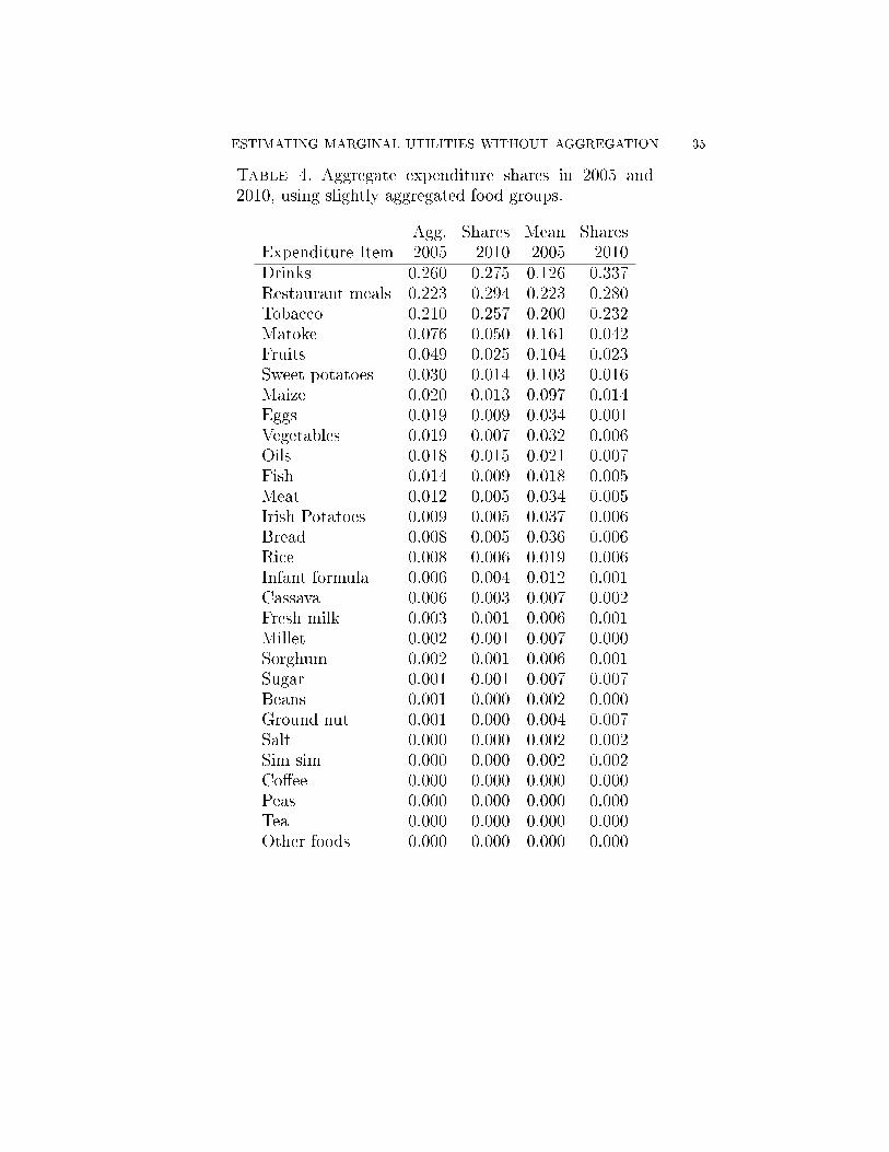
Table 4. Aggregate expenditure shares in 2005 and2010, using slightly aggregated food groups.

Agg. Shares Mean SharesExpenditure Item 2005 2010 2005 2010Drinks 0.260 0.275 0.126 0.337Restaurant meals 0.223 0.294 0.223 0.280Tobacco 0.210 0.257 0.200 0.232Matoke 0.076 0.050 0.161 0.042Fruits 0.049 0.025 0.104 0.023Sweet potatoes 0.030 0.014 0.103 0.016Maize 0.020 0.013 0.097 0.014Eggs 0.019 0.009 0.034 0.001Vegetables 0.019 0.007 0.032 0.006Oils 0.018 0.015 0.021 0.007Fish 0.014 0.009 0.018 0.005Meat 0.012 0.005 0.034 0.005Irish Potatoes 0.009 0.005 0.037 0.006Bread 0.008 0.005 0.036 0.006Rice 0.008 0.006 0.019 0.006Infant formula 0.006 0.004 0.012 0.001Cassava 0.006 0.003 0.007 0.002Fresh milk 0.003 0.001 0.006 0.001Millet 0.002 0.001 0.007 0.000Sorghum 0.002 0.001 0.006 0.001Sugar 0.001 0.001 0.007 0.007Beans 0.001 0.000 0.002 0.000Ground nut 0.001 0.000 0.004 0.007Salt 0.000 0.000 0.002 0.002Sim sim 0.000 0.000 0.002 0.002Co�ee 0.000 0.000 0.000 0.000Peas 0.000 0.000 0.000 0.000Tea 0.000 0.000 0.000 0.000Other foods 0.000 0.000 0.000 0.000

36 ETHAN LIGON

Figure 10. Aggregate expenditure shares in 2005 and2010, using slightly aggregated food groups.

Table 5. Aggregate expenditure shares in 2005 and2010, using more aggregated food groups.

Agg. Shares Mean SharesExpenditure Item 2005 2010 2005 2010Drinks 0.260 0.275 0.126 0.337Restaurant meals 0.223 0.294 0.223 0.280Stimulants 0.210 0.257 0.058 0.226Staples 1 0.145 0.087 0.418 0.082Fruits & Vegetables 0.067 0.032 0.137 0.029Proteins 0.046 0.023 0.087 0.011Oils, Salt, Sugar 0.020 0.016 0.030 0.016Staples 2 0.018 0.010 0.056 0.012Diary 0.010 0.005 0.018 0.002Legumes, etc. 0.002 0.001 0.008 0.009Other foods 0.000 0.000 0.000 0.000Total 1.001 1.0 1.161 1.004

A.5. Shares for Food in More Aggregated Groups.


Figure 11. Ratio of mean shares to aggregate shares,using slightly aggregated food groups. Items on the leftform a disproportionately large share of the budget ofthe rich; items on the right a disproportionately largebudget share of the needy.

38 ETHAN LIGON

Figure 12. Changes in mean shares across surveyrounds, using slightly aggregated food groups.


Figure 13. Aggregate expenditure shares in 2005 and2010, using more aggregated food groups.

Table 6. Aggregate expenditure shares in 2005 and2010, using CIOCOP groups.

Agg. Shares Mean SharesExpenditure Item 2005 2010 2005 2010Food 0.419 0.406 0.466 0.382Alcohol & Tobacco 0.371 0.462 0.578 0.498Housing & Utilities 0.116 0.078 0.224 0.071Health 0.043 0.022 0.062 0.022Other non-food 0.027 0.014 0.056 0.015Communication 0.014 0.013 0.012 0.010Transport 0.005 0.003 0.008 0.002Furnishing & ? 0.003 0.002 0.002 0.001Year 0.001 0.000 0.002 0.005Recreation 0.001 0.000 0.001 0.000Clothing & Footwear 0.000 0.000 0.000 0.000Education 0.000 0.000 0.000 0.000

A.6. Shares for Using COICOP Categories.

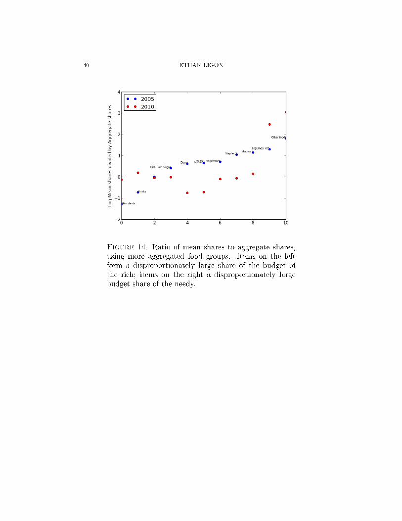
40 ETHAN LIGON

Figure 14. Ratio of mean shares to aggregate shares,using more aggregated food groups. Items on the leftform a disproportionately large share of the budget ofthe rich; items on the right a disproportionately largebudget share of the needy.


Figure 15. Changes in mean shares across surveyrounds, using more aggregated food groups.

42 ETHAN LIGON

Figure 16. Aggregate expenditure shares in 2005 and2010, using CIOCOP groups.


Figure 17. Ratio of mean shares to aggregate shares,using CIOCOP groups. Items on the left form a dispro-portionately large share of the budget of the rich; itemson the right a disproportionately large budget share ofthe needy.

44 ETHAN LIGON

Figure 18. Changes in mean shares across surveyrounds, using CIOCOP groups.

Documents

ESTIMATING MARGINAL UTILITIES WITHOUT AGGREGATION · ESTIMATING MARGINAL UTILITIES WITHOUT AGGREGATION ETHAN LIGON Contents 1. Introduction 1 2. A Wrong urnT 2 3. An Alternative Approach