Embed Size (px)
Citation preview

ESTIMATING PANEL DATA DURATION
MODELS WITH CENSORED DATA
Sokbae Lee
THE INSTITUTE FOR FISCAL STUDIES
DEPARTMENT OF ECONOMICS, UCL
cemmap working paper CWP13/03

Estimating Panel Data Duration Models with
Censored Data
Sokbae Lee ∗
Centre for Microdata Methods and PracticeInstitute for Fiscal Studies
andDepartment of EconomicsUniversity College LondonLondon, WC1E 6BT, UK
First Draft: September 2003
Revision: July 2005
Abstract
This paper presents a method for estimating a class of panel data duration models,under which an unknown transformation of the duration variable is linearly related tothe observed explanatory variables and the unobserved heterogeneity (or frailty) withcompletely known error distributions. This class of duration models includes a paneldata proportional hazards model with fixed effects. The proposed estimator is shownto be n1/2-consistent and asymptotically normal with dependent right censoring. Thepaper provides some discussions on extending the estimator to the cases of longer panelsand multiple states. Some Monte Carlo studies are carried out to illustrate the finite-sample performance of the new estimator.
Key words: Dependent censoring; frailty; panel data; recurrent events; survivalanalysis; transformation models.
∗I would like to thank Richard Blundell, Hide Ichimura, Roger Koenker, Bruce Meyer, Jeffrey Wooldridge(co-editor), two anonymous referees, and seminar participants at the 2003 Econometric Society North Amer-ican Summer Meeting, the CAM Workshop on Nonlinear Dynamic Panel Data Models, the LSE Joint Econo-metrics and Statistics Workshop, the Iowa Alumni Workshop, the department seminar at the University ofMannheim, and the UCL Econometrics Lunch Seminar for many helpful comments and suggestions. Anearlier version of the paper was circulated under the title “Semiparametric estimation of panel data durationmodels with fixed effects”.
1

Estimating Panel Data Duration Models with CensoredData
1 Introduction
Panel durations consist of multiple, sequentially observed durations of the same kind of
events on each individual. In a large number of applications across different scientific fields,
these panel durations are observed along with possible explanatory variables. Examples
of panel durations include recurrences of a given illness (Wei, Lin, and Weissfeld (1989)),
unemployment spells and job durations (Heckman and Borjas (1980), Topel and Ward
(1992)), birth intervals (Newman and McCullogh (1984)), car insurance claim durations
(Abbring, Chiappori, and Pinquet (2003)) and household inter-purchase times of a give
product (Jain and Vilcassim (1991)). This paper is concerned with estimating a class of
panel data duration models that can be viewed as panel data transformation models.
One econometric model that has been widely used in duration analysis is the mixed
proportional hazards model. This model is often defined in terms of the hazard function
of a positive random variable T (duration variable) conditional on a vector of observed
explanatory variables X (covariates) and an unobserved random variable U (the unobserved
heterogeneity or frailty). One form of this model is
λ(t|x, u) = λ0(t) exp(x′β + u), (1)
where λ(t|x, u) is the hazard that T = t conditional on X = x and U = u, the function λ0 is
the baseline hazard function, and β is the vector of unknown parameters. Here, x′ denotes
the transpose of x.
It is well known (see, for example, Section 4 of Van der Berg, 2001) that the mixed
proportional hazards model (1) can be written as the linear transformation model
log Λ0(T ) = −X ′β − U + ε, (2)
where Λ0(t) ≡∫ t0 λ0(u)du is the integrated baseline hazard function, and ε is an unob-
served random variable that is independent of X and U and has the type 1 extreme value
distribution function. The model (2) belongs to a class of linear transformation models
H(T ) = −X ′β − U + ε, (3)
2

where H(·) is an unknown strictly increasing function, and ε has a completely specified
distribution function F (·). If F is the type 1 extreme value distribution F (u) = 1−exp(−eu),
model (3) is the mixed proportional hazards model in (2). If F is the logistic distribution
F (u) = eu/(1+eu), model (3) can be called a mixed proportional odds model. For example,
see Cheng, Wei, and Ying (1995) and Horowitz (1996, 1998 Chap. 5) for detailed discussions
of applications of the transformation models.
This paper considers a panel data version of (3):
Hi(Tij) = −X ′ijβ − Ui + εij , (i = 1, . . . , n, j = 1, . . . , J), (4)
where i denotes an individual and j denotes a duration. For example, Tij denotes the i-th
individual’s j-th duration. It is assumed here that duration variables are successive and
observed sequentially. That is, Ti1 is followed by Ti2, which is followed by Ti3, and so on.
The observed covariates Xij are assumed to be constant within each spell but vary over
spells, whereas the unobserved heterogeneity Ui is assumed to be identical over spells. Thus,
Ui represents unobserved, permanent attributes of the i-th individual. Covariates that are
constant over spells are not included explicitly. They can be included in Ui, and their β
coefficients are not identified. We allow Ui to be arbitrarily correlated with Xij and do
not impose any distributional assumptions on Ui, and therefore, Ui is a fixed effect. Panel
data structure allows unobserved heterogeneity to have a very general form, compared to
unobserved heterogeneity in the single-spell duration models (e.g., Murphy, 1995).
It is also assumed that the unknown link function Hi(·) is strictly increasing but can be
different across individuals. Therefore, the model (4) allows for unobserved heterogeneity
in the shape of the link function as well. Finally, it is assumed that εij are independent of
Xij and independently and identically distributed (i.i.d.) across individuals and durations
with a completely specified distribution. As in the cross-sectional transformation model
(3), model (4) includes a panel data mixed proportional hazards model as a special case.
The focus of this paper is on estimating β in (4) when Tij is censored.1 It is well known
(see, e.g., Kalbfleisch and Prentice (1980, 8.1.2), Chamberlain (1985), Ridder and Tunalı
(1999), and Lancaster (2000)) that β can be estimated by a “stratified” partial likelihood
approach when Tij is uncensored or independently censored and F (u) = 1 − exp(−eu).1In this paper, we regard β as parameters of interest while we treat Hi nuisance parameters. To give a
specific example where β is of interest, consider a recent empirical work by Abbring, Chiappori, and Pinquet(2003). They test for moral hazard by checking whether car insurance claim intensities show negativeoccurrence dependence. This can be modelled semiparametrically in our setup by using dummy variablesfor panel durations of claims as part of X. A very general form of individual heterogeneity can be allowedby not specifying Hi.
3

The usefulness of the stratified partial likelihood approach for panel duration data would
be limited since dependent right censoring is almost inevitable in the analysis of panel
duration data. The standard independent censoring assumption is likely to be violated if
panel durations Tij are correlated. For example, see Visser (1996), Wang and Wells (1998),
and Lin, Sun, and Ying (1999) for discussions of the dependent censoring problem in terms
of estimating survivor functions without covariates.
The contribution of this paper is on developing an estimator of β when Tij is dependently
censored and F is known, not necessarily the type 1 extreme value distribution. Therefore,
this paper extends the transformation regression approach of Cheng, Wei, and Ying (1995)
to panel duration data and provides alternatives to the marginal regression approach of
Wei, Lin, and Weissfeld (1989). In a related paper, Horowitz and Lee (2004) developed an
estimator of β (among other things) when Tij is dependently censored, Hi(·) is the same
across individuals, and F (u) = 1 − exp(−eu). The proposed estimator in this paper is
based on a simple idea that the effect of censoring can be taken into account by using some
proper weights. The use of weighting is widespread in many contexts, and there are many
estimators based on weighting to deal with censoring. See for example, Koul, Susarla, and
Van Ryzin (1981) and Cheng, Wei, and Ying (1995) among many others.2
The paper is organized as follows. The next section describes the duration model and
gives an informal description of the estimator of β. Asymptotic properties of the proposed
estimator are given in Section 3. Extensions are discussed in Section 4. Section 5 presents
results of some Monte Carlo studies. Concluding remarks are in Section 6. The proof of
the main theorem is in Appendix.
2 Estimation of the Panel Data Duration Model
It is useful to begin with a description of the censoring mechanism. It is assumed in this
section that the number of durations J = 2. Let T1 and T2 be the duration variables of two
consecutive and adjacent events. For J = 2, the model (4) has the form
H(T1) = −X ′1β − U + ε1 and H(T2) = −X ′
2β − U + ε2. (5)
Censoring is an inevitable part of modelling in duration analysis. To describe a censoring
mechanism for successive durations T1 and T2, we assume that T1 and T2 are observed2See equations (3.51) and (3.52) of Powell (1994, p.2505) for a concise explanation of the idea behind the
estimator of Koul, Susarla, and Van Ryzin (1981).
4

consecutively over a time period C, where C is random with an unknown probability distri-
bution. As discussed in Visser (1996) and Wang and Wells (1998), there are three possible
cases:
(1) if C ≥ T1 + T2, both T1 and T2 are uncensored;
(2) if T1 ≤ C < T1 + T2, T1 is uncensored but T2 is censored;
(3) if C < T1, T1 is censored and T2 is unobserved.
Notice that T1 is censored by C1 ≡ C and that T2 is censored by C2 ≡ (C1 − T1)1(T1 ≤C1), where 1(·) is the usual indicator function. Under this censoring mechanism, C2 is
correlated with T2 because T1 and T2 are correlated by unobserved heterogeneity. This
indicates that it would be quite difficult to estimate a (cross-sectional) duration model for
T2 in separation from T1 with censored data. However, we will show below that β in (4)
can be estimated consistently.
To do so, we assume that one observes a pair of (Yj , ∆j) not Tj , where Yj = min(Tj , Cj)
and ∆j = 1(Tj ≤ Cj) for j = 1, 2. The observed data consist of i.i.d. realizations
(Yi1, Yi2, Xi1, Xi2, ∆i1,∆i2) : i = 1, . . . , n from (Y1, Y2, X1, X2, ∆1,∆2). Let G(c) denote
the survivor function of C, that is G(c) = Pr(C ≥ c), and let ∆X = X1 − X2. Assume
that C is independent of (T1, T2, X1, X2, U). Let L(u) = Pr[(ε1− ε2) > u] for any real value
u. Also, let l(u) = −dL(u)/du, that is l(·) is the probability density function of (ε1 − ε2).
Then if we assume that ε1 and ε2 are independently and identically distributed with the
common distribution function F ,
L(u) =∫ ∞
−∞[1− F (u + v)]dF (v). (6)
Assume further that ε1 and ε2 are independent of X1 and X2. Notice that under these
assumptions made above,
E
[∆1∆2
G(Y1 + Y2)
1(Y1 > Y2)− L(∆X ′β)
∣∣∣∣X1, X2
]
= E
[E
[1(T1 + T2 ≤ C)
G(T1 + T2)
1(T1 > T2)− L(∆X ′β)
∣∣∣∣T1, T2, X1, X2
]∣∣∣∣X1, X2
]
= E[1(T1 > T2)− L(∆X ′β)
∣∣X1, X2
]
= E[1H(T1) > H(T2) − L(∆X ′β)
∣∣X1, X2
]
= Pr[(ε1 − ε2) > (X1 −X2)′β
∣∣X1, X2
]− L(∆X ′β)
= 0. (7)
5

This implies that β satisfies the moment condition
E
wh(∆X ′β)∆X
∆1∆2
G(Y1 + Y2)
[1(Y1 > Y2)− L(∆X ′β)
]= 0, (8)
where wh(·) is a weight function.3
Our estimation strategy in this paper is to solve the sample analog of the population
moment condition (8). In other words, our estimator bn of β is the solution to the following
estimating equation
n−1n∑
i=1
wh(∆X ′
ib)∆Xi∆i1∆i2
Gn(Yi1 + Yi2)
[1(Yi1 > Yi2)− L(∆X ′
ib)]
= 0, (9)
where Gn is an estimator of G. Since C is censored independently by T1 + T2, we will use
the Kaplan-Meier estimator of G for Gn. Specifically, Gn is estimated based on the data
(Yi1 + Yi2, 1−∆i1∆i2) : i = 1, . . . , n.4We end this section by mentioning some connection to well-known estimation methods.
If wh(·) = l(·)/L(·)[1−L(·)], the estimator defined in (9) can be thought of as a weighted
maximum-likelihood type estimator, meaning that bn is the solution to
maxb
n−1n∑
i=1
∆i1∆i2
Gn(Yi1 + Yi2)
1(Yi1 > Yi2) log[L(∆X ′
ib)] + 1(Yi1 ≤ Yi2) log[1− L(∆X ′ib)]
.
When F is the type 1 extreme value distribution function, it can be seen that the proposed
estimator is a weighted logit estimator with weight equal to the inverse of the probability
that T1 and T2 are uncensored.
3 Asymptotic Properties of the Estimator
This section establishes the n−1/2-consistency and asymptotic normality of bn. To do so,
we make the following assumptions:
Assumption 1. β is an interior point of the parameter space B, which is a compact subset
of Rd.3Obviously there are other moment conditions that can be derived from (7). It may be useful to develop
a more efficient GMM-type estimator using a set of possible moment conditions; however, it is beyond thescope of this paper to investigate the issue of efficiency.
4Since C is also censored independently by T1, the Kaplan-Meier estimator Gn could be estimated basedon the data (Yi1, 1−∆i1) : i = 1, . . . , n as well.
6

Assumption 2. The data (Yi1, Yi2, Xi1, Xi2,∆i1, ∆i2) : i = 1, . . . , n are i.i.d. realizations
from (Y1, Y2, X1, X2,∆1, ∆2) in (5).
It is possible that Xi1 and Xi2 are missing when durations of interest are censored,
especially when Xi1 and Xi2 are observed characteristics of durations. This does not cause
any problem for the estimation procedure in Section 2 because the estimating equation (9)
mainly uses observations corresponding to complete durations (that is, ∆i1 = ∆i2 = 1).
Observations with incomplete durations are only used to obtain an estimator of G to take
into the account of the effect of dependent right censoring. Since C is independent of X1
and X2, it is unnecessary to observe X1 and X2 when durations are censored.
Assumption 3. (1) ε1 and ε2 have the same distribution function F (·), which is com-
pletely specified. (2) There exists a corresponding probability density function f(·), which is
bounded, continuous, and positive everywhere along the real line. (3) Furthermore, ε1 and
ε2 are independent of each other and independent of (X1, X2).
As already discussed, this condition is satisfied by the panel data proportional hazards
model with unobserved heterogeneity.
Assumption 4. The function H(·) is strictly increasing.
It can be seen from (7) that the link function H(·) can be different across individuals.
This allows for arbitrary heterogeneity in the shape of the link function. As a matter of fact,
U is not identified from H(·) since H(·) can vary over individuals. However, the model is
expressed in the form of (4) to emphasize connections between our model (4) and duration
models with unobserved heterogeneity.5
Assumption 5. The weight function wh(·) is bounded and positive everywhere along the
real line and has a bounded, continuous derivative.
A simple choice of wh would be to set wh ≡ 1. As suggested by Cheng, Wei, and Ying
(1985), one might use wh(·) = l(·)/L(·)[1− L(·)] to mimic the quasi-likelihood approach.
Let ‖‖ denote the Euclidean norm.
Assumption 6. E ‖∆X‖4 < ∞ and E[∆X∆X ′] is nonsingular.5The stratified partial likelihood approach also allows the baseline hazard function to vary over individ-
uals. See, for example, Chamberlain (1985) and Ridder and Tunalı (1999) for details.
7
This condition requires that covariates vary over spells, thereby excluding the constant
term and spell-constant covariates.6
Assumption 7. (1) The censoring variable C is random with an unknown continuous
probability distribution. In addition, C is independent of (T1, T2, X1, X2, U).
(2) The survivor function of C, G(c) ≡ Pr(C ≥ c) is positive for every c ∈ R.
Assumption 7 (1) is a convenient assumption under which we utilize results of counting
process and martingale methods for the Kaplan-Meier estimator of G(·).7 Assumption 7
(2) is a rather strong condition and especially it excludes the case of fixed censoring.8 The
same condition is assumed in Koul, Susarla, and Van Ryzin (1981, Assumption A1).
To present our main result, define π(s) = Pr(Y1 + Y2 ≥ s) and
Mi(s) = 1(Yi1 + Yi2 ≤ s,∆i1∆i2 = 0)−∫ s
01(Yi1 + Yi2 ≥ c) dΛC(c),
where ΛC is the cumulative hazard function of C. In addition, define
Ω = E[wh(∆X ′β)l(∆X ′β)∆X∆X ′]
and
ϕ(Yi1, Yi2, Xi1, Xi2, ∆i1, ∆i2)
= wh(∆X ′iβ)∆Xi
∆i1∆i2
G(Yi1 + Yi2)
[1(Yi1 > Yi2)− L(∆X ′
iβ)]
+∫ ∞
0
Γ(s)π(s)
dMi(s),
where
Γ(s) = E
wh(∆X ′β)∆X
∆1∆2
G(Y1 + Y2)
[1(Y1 > Y2)− L(∆X ′β)
]1(Y1 + Y2 ≥ s)
.
The following theorem provides the main result of the paper.6As is common among fixed-effects estimators, if regression coefficients of spell-constant covariates vary
over spells, then the difference between two coefficients can be identified and estimated using the methoddeveloped in this paper.
7See, for example, Assumption 6.2.2 of Fleming and Harrington (1991, p.232). In principle, one couldallow C to depend on X1 and X2. This would make the estimator and asymptotic theory more complicatedsince the conditional Kaplan-Meier estimator is then needed. See, e.g., Dabrowska (1989) for details of theconditional Kaplan-Meier estimator.
8Roughly speaking, this assumption requires that there is a chance of observing a complete spell nomatter how large the spell is. This might not be palatable in some applications, so that we carry out MonteCarlo experiments that investigate how the proposed estimator performs when Assumption 7 (2) is violated.
8

Theorem 1. Let Assumptions 1-7 hold. Then
n1/2(bn − β) = −n−1/2n∑
i=1
Ω−1ϕ(Yi1, Yi2, Xi1, Xi2, ∆i1, ∆i2) + op(1).
In particular, n1/2(bn − β) is asymptotically normal with mean zero and covariance matrix
Vβ ≡ Ω−1ΦΩ−1, where
Φ = E
[[wh(∆X ′β)]2∆X∆X ′ ∆1∆2
[G(Y1 + Y2)]2L(∆X ′β)[1− L(∆X ′β)]
]−
∫ ∞
0
Γ(s)Γ(s)′
π(s)dΛC(s).
Notice that the covariance matrix Vβ is smaller (in the matrix sense) than one that would
be obtained with a true G(·) instead of an estimated Gn(·).9 It is straightforward to obtain
a consistent estimator of the covariance matrix Vβ. Define π(s) = n−1∑n
i=1 1(Yi1 +Yi2 ≥ s)
and
Γ(s) = n−1n∑
i=1
wh(∆X ′
ibn)∆Xi∆i1∆i2
Gn(Yi1 + Yi2)
[1(Yi1 > Yi2)− L(∆X ′
ibn)]1(Yi1 + Yi2 ≥ s)
.
One can estimate Vβ by its sample analog estimator Vβ = Ω−1ΦΩ−1, where
Ω = n−1n∑
i=1
wh(∆X ′ibn)
∆i1∆i2
[Gn(Yi1 + Yi2)]l(∆X ′
ibn)∆Xi∆X ′i,
and
Φ = n−1n∑
i=1
[wh(∆X ′ibn)]2∆Xi∆X ′
i
∆i1∆i2
[Gn(Yi1 + Yi2)]2L(∆X ′
ibn)[1− L(∆X ′ibn)]
− n−1n∑
i=1
(1−∆i1∆i2)Γ(Yi1 + Yi2)Γ(Yi1 + Yi2)′
[π(Yi1 + Yi2)]2.
Notice that the second term of Φ is a sample analog of the second term of Φ using the
Nelson cumulative hazard estimator of ΛC .10
9This result is not surprising; see, for example, Koul, Susarla, and Van Ryzin (1981), Srinivasan andZhou (1994) and Cheng, Wei, and Ying (1995) for cases of smaller asymptotic variances with estimated Gn.See, also, Wooldridge (2002) for similar results in the context of inverse probability weighted M-estimationfor general selection problems.
10One could estimate Ω using Ω, where Ω is the same as Ω without the weighting term ∆i1∆i2/Gn(Yi1 +Yi2). Instead we decide to use Ω because it is expected that due to the use of weighting, Ω might have asmaller variance than Ω. This conjecture was confirmed by a small Monte Carlo experiment, although wedid not calculate the asymptotic variances of Ω and Ω.
9
4 Extensions
4.1 Estimation with Longer Panels
The estimation method in Section 2 easily extends to the case of longer panels. To consider
estimation when J > 2, it is important to notice that panel durations Tij in (4) are censored
by Cij , where Ci1 = Ci and Cij = (Ci −∑j−1
k=1 Tik)1(Ti,j−1 ≤ Ci,j−1) for j = 2, . . . , J . As
before, one observes Yij = min(Tij , Cij) and ∆ij = 1(Tij ≤ Cij) together with covariates
Xij for j = 1, . . . , J and i = 1, . . . , n. Using the fact that the sum of Tij ’s is censored
independently by C, the estimating equation (9) can be extended to longer panels. To do
so, let S be a set of pairs of indices such that S = (j, k) : j < k, j = 1, . . . , J, k = 1, . . . , J,∆ijk = Xij −Xik, and Wij =
∑jk=1 Yik, that is the sum of the first j observed spells. Then
an estimator of β is the solution to the following estimating equation
n−1n∑
i=1
∑
(j,k)∈S
wh(∆X ′
ijkb)∆Xijk∆ij∆ik
Gn(Wik)
[1(Yij > Yik)− L(∆X ′
ijkb)]
= 0. (10)
As in Section 2, the effect of censoring is adjusted by multiplying the inverse of the estimates
Gn(Wik) of the probability that Yij and Yik are uncensored for j < k. It is straightforward
to obtain asymptotic properties of this estimator.
4.2 Estimation with Multiple States
This subsection shows how the estimation method in Section 2 can be extended to the
case of multiple-state duration models. The censoring mechanism described in Section 2
considers a pure renewal process in the sense that T1 and T2 are the durations of the same
kind and there is no time spent on other states. This pure renewal process assumption
might be implausible in some applications, for example, employment and unemployment
durations in labor economics. Fortunately, it is easy to extend the estimation method in
Section 2 to multiple-state duration models.
Assume now that there is a different type of duration between two durations of interest,
say T . For example, T1 may be the duration of the first job, T the duration of being
unemployed or out of labor force, and T2 the duration of the second job. Assume that C
is independent of T1, T2, X1, X2, and T . One observes uncensored durations of T1 and
T2 when C ≥ T1 + T + T2. Hence, ∆i1∆i2 = 1(Ci ≥ Ti1 + Ti + Ti2). Then a consistent
estimator of β can be obtained by solving the same estimating equation as (9), except that
Gn(Yi1 + Yi2) is now replaced with Gn[min((Ti1 + Ti + Ti2), Ci)].
10

Basically, the estimation method in Section 2 can be extended to any censoring mecha-
nism, provided that the probability of at least two durations of interest being uncensored is
positive and can be estimated consistently. The main idea behind the estimation method
is to use only observations corresponding to complete durations and to correct for the in-
duced selection bias by using proper weights, namely the inverse of the probability of two
durations being uncensored.
5 Monte Carlo Studies
This section presents the results of some simulation studies that illustrate the finite-sample
performance of the estimator. For each Monte Carlo experiment, 1,000 samples were gen-
erated from the following model with J = 2:
H(T1) = −X11β1 −X12β2 −X13β3 − U + ε1,
H(T2) = −X21β1 −X22β2 −X23β3 − U + ε2,
where H is the natural log function, X11 and X21 were independently drawn from a uniform
distribution on [0,1], X12 and X22 were independent dummy variables with being equal to
one with probability 0.5, X13 and X23 were also dummy variables such that X31 = 0 and
X32 = 1, and ε1 and ε2 were independently drawn from the type 1 extreme value dis-
tribution. The unobserved heterogeneity U was generated by U = (X11 + X21)/2 and is
the only source of correlation between T1 and T2. The true parameters are (β1, β2, β3) =
(−1,−1,−1). Finally, we experiment with two types of distributions for the censoring mech-
anism. Firstly, the censoring threshold C was generated from the exponential distribution
with mean µ, and secondly, C was from the uniform distribution with support [0, ν], where
different µ’s and ν’s were chosen to investigate the effects of censoring. Assumption 7 (2)
is satisfied by the exponential distribution, but not by the uniform distribution. The lat-
ter distributed is considered to see how the estimator performs when Assumption 7 (2)
is violated. The simulations used sample sizes of n = 100, 200, 400 and 800, and all the
simulations were carried out in GAUSS using GAUSS pseudo-random number generators.
Throughout the simulations, the weight function was wh ≡ 1.
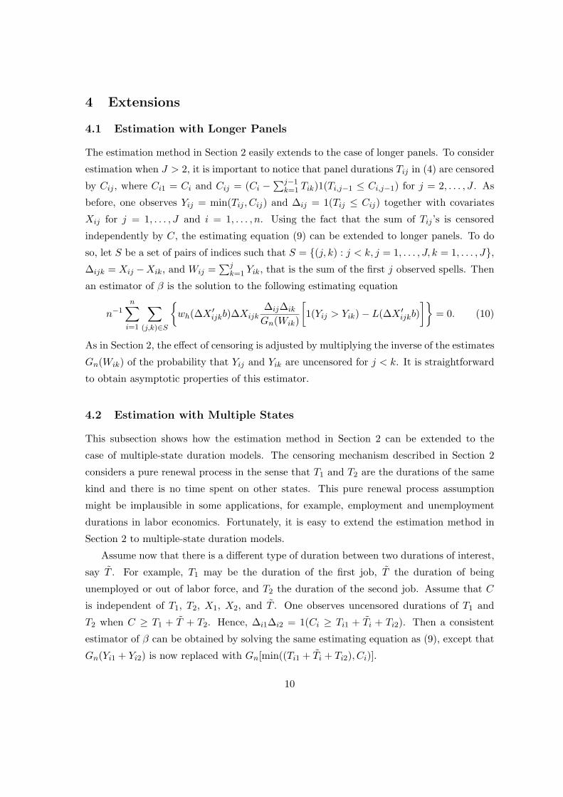
Table 1 reports the mean bias and standard deviation (S.D.) for the estimate of each
coefficient for the case of censoring with the exponential distribution. It can be seen that
for each coefficient and for each level of censoring, the bias is negligible. Furthermore, the
standard deviation decreases quite quickly as the sample size increases about a rate of n−1/2,
11

although the estimator does not perform well when the proportion of censoring exceeds 50%.
Table 2 reports the mean bias and standard deviation for the estimate of each diagonal
component of the variance matrix Vβ/n. To compute the biases and standard deviations,
the finite-sample variances of estimates of coefficients (obtained by 1000 simulations) are
treated as the true values of the variances. Again the variance estimator performs well
except for heavy censoring. Note that the standard deviation shrinks quite fast with the
sample size because the true variance also shrinks.
We now consider the case of censoring with the uniform distribution. The results are
summarized in Tables 3 and 4. Not surprisingly, the performance of the estimator is worse
compared to the case with the exponential distribution. Note that the asymptotic biases
are quite small for light censoring (up to 30%) and they get larger for heavier censoring.
Similar conclusions can be drawn for variance estimates.
In summary, our simulation results suggest that (1) the new estimator and its variance
estimator perform very well in finite samples for light and moderate censoring (up to 50%)
when the censoring variable has infinite support, (2) they perform quite well for light cen-
soring (up to 30%) when the censoring variable has finite support, and (3) the performance
deteriorates rapidly as the proportion of censoring exceeds 50% for both cases of censoring.
In view of these results, we recommend the new estimator when the censoring involves less
than 50% of observations, especially with small sample sizes.
6 Conclusions
This paper has considered the estimation of panel data duration models with unobserved
heterogeneity. In particular, this paper has provided a method for estimating the regression
coefficients under dependent right censoring. The new estimator has its strengths and
weaknesses. The strengths are that the estimator is fairly easy to implement and can
be extended easily to the cases of longer panels and multiple states. However, there are
weaknesses regarding the regularity conditions on the censoring variable. The new estimator
may not be consistent without infinite support for the censoring variable; however, when
this assumption is not satisfied, the estimator performs pretty well in the Monte Carlo
experiments for the cases with light censoring (up to 30% of observations).
Another possible extension that is not included in Section 4 is to let F (·) be unknown.
Under this generalization, (7) can be thought of as a single index mean regression model,
in which ∆1∆2G(Y1+Y2)1(Y1 > Y2) is the dependent variable. Thus, it is expected that β can
12

be estimated (up to scale) at a n−1/2 rate by combining methods similar to those used in
the analysis of single index models (see, e.g., Ichimura (1993), Klein and Spady (1993),
Powell, Stock, and Stoker (1989), Horowitz and Hardle (1996), and Hristache, Juditski,
and Spokoiny (2001)) with some tail behavior restrictions on the Kaplan-Meier estimator
of G(·). This is a topic for future research.
Appendix: Proof of Theorem 1
It is assumed in Appendix that Assumptions 1-7 hold. The following lemma is useful to
prove Theorem 1.
Lemma 1. Let Sn(b) denote the left-hand side of (9). Then Sn(b) converges uniformly in
probability to S0(b), where
S0(b) = E
[wh(∆X ′b)∆X
L(∆X ′β)− L(∆X ′b)
].
Proof of Lemma 1. Define Cn = maxiYi1 + Yi2. For any value of τ > 0, write Sn(b) =
Sn1(b; τ) + Sn2(b; τ), where
Sn1(b; τ) = n−1n∑
i=1
wh(∆X ′
ib)∆Xi1(Yi1 + Yi2 ≤ τ)∆i1∆i2
Gn(Yi1 + Yi2)
[1(Yi1 > Yi2)− L(∆X ′
ib)]
and
Sn2(b; τ) = n−1n∑
i=1
wh(∆X ′
ib)∆Xi1(τ < Yi1 + Yi2 ≤ Cn)∆i1∆i2
Gn(Yi1 + Yi2)
[1(Yi1 > Yi2)− L(∆X ′
ib)]
.
Let Sn(b) denote the same expression as Sn(b) except that Gn(Yi1 + Yi2) is replaced with
G(Yi1 + Yi2), so that Sn(b) = Sn1(b; τ) + Sn2(b; τ), where
Sn1(b; τ) = n−1n∑
i=1
wh(∆X ′
ib)∆Xi1(Yi1 + Yi2 ≤ τ)∆i1∆i2
G(Yi1 + Yi2)
[1(Yi1 > Yi2)− L(∆X ′
ib)]
and
Sn2(b; τ) = n−1n∑
i=1
wh(∆X ′
ib)∆Xi1(τ < Yi1 + Yi2 ≤ Cn)∆i1∆i2
G(Yi1 + Yi2)
[1(Yi1 > Yi2)− L(∆X ′
ib)]
.
First, consider the limiting behavior of Sn1(b; τ). Notice that supc : G(c) > 0 = ∞.
Thus, by the property of Kaplan-Meier estimator (see, for example, Fleming and Harrington,
1991), Gn(c) converges to G(c) uniformly on [0, τ ] and Gn(c) : c ∈ [0, τ ] and G(c) : c ∈
13

[0, τ ] are bounded away from zero for sufficiently large n for any fixed but arbitrary τ > 0.
This implies that
|Sn1(b; τ)− Sn1(b; τ)| ≤ supi
∣∣∣∣1(Yi1 + Yi2 ≤ τ)
G(Yi1 + Yi2)G(Yi1 + Yi2)−Gn(Yi1 + Yi2)
Gn(Yi1 + Yi2)
∣∣∣∣
× n−1n∑
i=1
‖∆Xi‖ 2|wh(∆X ′ib)|
= op(1)Op(1) = op(1)
uniformly over (b, τ). In addition, since G(c) : c ∈ [0, τ ] is bounded away from zero, by
uniform laws of large numbers (e.g., Lemma 2.4 of Newey and McFadden, 1994, p.2129),
Sn1(b; τ) converges uniformly over (b, τ) in probability to S01(b; τ), where
S01(b; τ) = E
[wh(∆X ′b)∆X1(T1 + T2 ≤ τ)
L(∆X ′β)− L(∆X ′b)
].
Next, consider the limiting behavior of Sn2(b; τ). We will show in the below that this
term is negligible for a large τ using arguments similar to those used in Srinivasan and Zhou
(1994, Section 5). Notice that
|Sn2(b; τ)− Sn2(b; τ)| ≤ supYi1+Yi2≤Cn
∣∣∣∣G(Yi1 + Yi2)−Gn(Yi1 + Yi2)
Gn(Yi1 + Yi2)
∣∣∣∣
× n−1n∑
i=1
∣∣∣∣1(Yi1 + Yi2 > τ)∆i1∆i2
G(Yi1 + Yi2)
∣∣∣∣ ‖∆Xi‖ 2|wh(∆X ′ib)|.
(11)
By Zhou (1991, Theorem 2.2),
supc<Cn
∣∣∣∣G(c)−Gn(c)
Gn(c)
∣∣∣∣ = Op(1). (12)
Taking Gn(·) to be a left-continuous version of the Kaplan-Meier estimator (i.e. Gn(·−) =
Gn(·); see, also, equation (5.7) of Srinivasan and Zhou, 1994),
supYi1+Yi2≤Cn
∣∣∣∣G(Yi1 + Yi2)−Gn(Yi1 + Yi2)
Gn(Yi1 + Yi2)
∣∣∣∣ = Op(1). (13)
14

By Markov inequality, for any M > 0 and for any τ > 0,
Pr
(n−1
n∑
i=1
1(Yi1 + Yi2 > τ)∆i1∆i2
[G(Yi1 + Yi2)]‖∆Xi‖ > M
)
= Pr
(n−1
n∑
i=1
1(Ti1 + Ti2 > τ)∆i1∆i2
[G(Ti1 + Ti2)]‖∆Xi‖ > M
)
≤ M−1E
[1(T1 + T2 > τ)
∆1∆2
G(T1 + T2)‖∆X‖
]
= M−1E [ 1(T1 + T2 > τ) ‖∆X‖ ]
≤ M−1(E[1(T1 + T2 > τ)])1/2(E ‖∆X‖2)1/2.
(14)
Combing (13) and (14) with (11) gives that
|Sn2(b; τ)− Sn2(b; τ)| = Op(1) (15)
uniformly over b for any τ . In view of (14), it can also be shown that
|Sn2(b; τ)− S02(b; τ)| = Op(1) (16)
uniformly over b for any τ , where
S02(b; τ) = E
[wh(∆X ′b)∆X1(T1 + T2 > τ)
L(∆X ′β)− L(∆X ′b)
].
Thus, (15) and (16) imply that |Sn2(b; τ)−S02(b; τ)| can be arbitrarily small by choosing a
large τ . Therefore, we have proved the lemma.
Proof of Theorem 1. It is obvious that S0(b) is continuous and is zero only when b = β.
Therefore, in view of Lemma 1, bn is consistent, i.e. bn →p β.
Now a first-order Taylor series approximation of Sn(bn) at β gives
0 = n1/2Sn(bn) = n1/2Sn(β) +∂Sn(b∗n)
∂bn1/2(bn − β), (17)
where b∗n is between bn and β, and ∂Sn/∂b is the matrix whose (l, k) element is the partial
derivative of the l-th component of Sn with respect to the k-th component of b. Let
wh(u) = dwh(u)/du. Notice that for any b,
∂Sn(b)∂b
= Tn1(b) + Tn2(b),
15

where
Tn1(b) = n−1n∑
i=1
wh(∆X ′ib)
∆i1∆i2
Gn(Yi1 + Yi2)l(∆X ′
ib)∆Xi∆X ′i
and
Tn2(b) = n−1n∑
i=1
wh(∆X ′
ib)∆Xi∆X ′i
∆i1∆i2
Gn(Yi1 + Yi2)
[1(Yi1 > Yi2)− L(∆X ′
ib)]
.
By arguments similar to those used to prove Lemma 1 with the assumption that E ‖∆X‖4 <
∞, we have
supb∈B
∥∥Tn1 − E[wh(∆X ′b)l(∆X ′b)∆X∆X ′]∥∥ = op(1)
and
supb∈B
∥∥∥Tn2 − E[wh(∆X ′b)∆X∆X ′(L(∆X ′β)− L(∆X ′b)
)]∥∥∥ = op(1).
Therefore, an application of the continuous mapping theorem yields∥∥∥∥∥∂Sn(b∗n)
∂b− Ω
∥∥∥∥∥ = op(1). (18)
Now consider n1/2Sn(β). Using the same notation as in the proof of Lemma 1, write
Sn(β) = Sn1(β; τ) + Sn2(β; τ). That is,
Sn1(β; τ) = n−1n∑
i=1
wh(∆X ′
iβ)∆Xi1(Yi1 + Yi2 ≤ τ)∆i1∆i2
Gn(Yi1 + Yi2)
[1(Yi1 > Yi2)− L(∆X ′
iβ)]
and
Sn2(β; τ) = n−1n∑
i=1
wh(∆X ′
iβ)∆Xi1(Yi1 + Yi2 > τ)∆i1∆i2
Gn(Yi1 + Yi2)
[1(Yi1 > Yi2)− L(∆X ′
iβ)]
.
For any c ≤ τ , by a martingale integral representation for the Kaplan-Meier estimator (see,
for example, Fleming and Harrington, 1991),
G(c)−Gn(c)Gn(c)
= n−1n∑
k=1
∫ ∞
0
1(c ≥ s)π(s)
dMk(s) + op(n−1/2),
where π(s) and Mk(s) are defined in the main text. Using this, we have
Sn1(β; τ) = Sn1(β; τ) + Rn1(β; τ) + op(n−1/2)
16

for any arbitrary but fixed τ , where
Sn1(β; τ) = n−1n∑
i=1
S1i(β; τ),
Rn1(β; τ) = n−1n∑
k=1
∫ ∞
0n−1
n∑
i=1
Sn1i(β; τ)1
π(s)dMk(s),
and
S1i(β; τ) = wh(∆X ′iβ)∆Xi1(Yi1 + Yi2 ≤ τ)
∆i1∆i2
G(Yi1 + Yi2)
[1(Yi1 > Yi2)− L(∆X ′
iβ)].
Then standard arguments for obtaining the projection of a U-statistic (see, for example,
Lemma 8.4 of Newey and McFadden, 1994, p.2201) gives
Rn1(β; τ) = n−1n∑
k=1
∫ ∞
0
Γ(s)π(s)
dMk(s) + op(n−1/2),
where
Γ(s; τ) = E
wh(∆X ′β)∆X1(Y1 + Y2 ≤ τ)
∆1∆2
G(Y1 + Y2)
[1(Y1 > Y2)− L(∆X ′β)
]1(Y1 + Y2 ≥ s)
Now consider the tail part, i.e. Sn2(β; τ). Write
Sn2(β; τ) = Sn2(β; τ) + Rn21(β; τ) + Rn22(β; τ), (19)
where
S2i(β; τ) = wh(∆X ′iβ)∆Xi1(Yi1 + Yi2 > τ)
∆i1∆i2
G(Yi1 + Yi2)
[1(Yi1 > Yi2)− L(∆X ′
iβ)],
Sn2(β; τ) = n−1n∑
i=1
S2i(β; τ),
Rn21(β; τ) = n−1n∑
i=1
Sn2i(β; τ)G(Yi1 + Yi2)−Gn(Yi1 + Yi2)
G(Yi1 + Yi2),
and
Rn22(β; τ) = n−1n∑
i=1
Sn2i(β; τ)[G(Yi1 + Yi2)−Gn(Yi1 + Yi2)]2
G(Yi1 + Yi2)Gn(Yi1 + Yi2).
In view of Theorem 2.1 of Gill (1983),
supYi1+Yi2≤Cn
∣∣∣∣G(Yi1 + Yi2)−Gn(Yi1 + Yi2)
G(Yi1 + Yi2)
∣∣∣∣ = Op(n−1/2).
17

Using this and (13), we can show that each term in (19) is of order Op(n−1/2) for any τ . This
implies that Sn2(β; τ) can be of order op(n−1/2) by taking τ sufficiently large. Therefore,
combining results above with a choice of a sufficiently large τ gives the first conclusion of
the theorem.
It now remains to calculate the asymptotic variance, in particular Φ. First, note that
by the variance calculation for a martingale (see, e.g., Theorems 2.4.5 and 2.5.4 of Fleming
and Harrington, 1991),
var∫ ∞
0
Γ(s)π(s)
dMi(s)
=∫ ∞
0
Γ(s)Γ(s)′
π(s)dΛC(s).
Furthermore,
2cov
wh(∆X ′iβ)∆Xi
∆i1∆i2
G(Yi1 + Yi2)
[1(Yi1 > Yi2)− L(∆X ′
iβ)],
∫ ∞
0
Γ(s)′
π(s)dMi(s)
= −2cov
wh(∆X ′iβ)∆Xi
∆i1∆i2
G(Yi1 + Yi2)
[1(Yi1 > Yi2)− L(∆X ′
iβ)],
∫ ∞
01(Yi1 + Yi2 ≥ s)
Γ(s)′
π(s)dΛc(s)
= −2∫ ∞
0
Γ(s)Γ(s)′
π(s)dΛC(s).
Then the second conclusion of the theorem follows immediately.
References
Abbring, J.H, P.A, Chiappori, and J. Pinquet (2003) Moral hazard and dynamic insurance
data, 1, 767-820.
Chamberlain, G. (1985) Heterogeneity, omitted variable bias, and duration dependence,
in: J.J. Heckman and B. Singer, eds. Longitudinal analysis of labor market data
(Cambridge University Press, Cambridge) 3-38.
Cheng, S.C., L.J. Wei, and Z. Ying (1995) Analysis of transformation models with censored
data, Biometrika, 82, 835-845.
Dabrowska, D., 1989, Uniform consistency of the kernel conditional Kaplan-Meier estimate,
Annals of Statistics, 17, 1157-1167.
Fleming, T.R., and D.P. Harrington, 1991, Counting processes and survival analysis (Wi-
ley, New York).
18

Gill, R. (1983) Large sample behaviour of the product-limit estimator on the whole line,
Annals of Statistics, 11, 49-58.
Heckman, J.J., and G.J. Borjas (1980) Does unemployment cause future unemployment?
definitions, questions and answers for a continuous time model of heterogeneity and
state dependence, Economica, 47, 247-283.
Honore, B.E. (1990) Simple estimation of a duration model with unobserved heterogeneity,
Econometrica, 58, 453-473.
Honore, B.E. (1993) Identification results for duration models with multiple spells, Review
of Economic Studies, 60, 241-246.
Horowitz, J.L. (1996) Semiparametric estimation of a regression model with an unknown
transformation of the dependent variable, Econometrica, 64, 103-137.
Horowitz, J.L. (1998) Semiparametric methods in econometrics (Springer-Verlag, New
York).
Horowitz, J.L., and W. Hardle (1996) Direct semiparametric estimation of single-index
models with discrete covariates, Journal of the American Statistical Association, 91,
1632-1640.
Horowitz, J.L., and S. Lee (2004) Semiparametric estimation of a panel data proportional
hazards model with fixed effects, Journal of Econometrics, 119, 155-198.
Hristache, M., A. Juditski, and V. Spokoiny (2001) Direct estimation of the index coeff-
cients in a single index model, Annals of Statistics, 29, 595-623.
Ichimura, H. (1993) Semiparametric least squares (SLS) and weighted SLS estimation of
single index models, Journal of Econometrics, 58, 71-120.
Jain, D., and N.J. Vilcassim (1991) Investigating household purchase timing decisions: a
conditional hazard function approach, Marketing Science, 10, 1-23.
Kalbfleisch, J.D., and R.L. Prentice (1980) The statistical analysis of failure time data
(Wiley, New York).
Klein, R.W., and R.H. Spady (1993) An efficient semiparametric estimation for binary
response models, Econometrica, 61, 387-421.
19

Koul, H., V. Susarla, and J. Van Ryzin (1981) Regression analysis with randomly right-
censored data, Annals of Statistics, 9, 1276-1288.
Lancaster, T. (2000) The incidental parameter problem since 1948, Journal of Economet-
rics, 95, 391-413.
Lin, D.Y., W. Sun, and Z. Ying (1999) Nonparametric estimation of the gap time distrib-
utions for serial events with censored data, Biometrika, 86, 59-70.
Murphy, S. A. (1995) Asymptotic theory for the frailty model, Annals of Statistics, 23,
182-198.
Newey, W.K., and D.L. McFadden (1994) Large Sample Estimation and Hypothesis Test-
ing, in: R.F. Engle and D.L. McFadden, eds. Handbook of Econometrics, Vol IV.
(North-Holland, Amsterdam) Chapter 36.
Newman, J.L., and C.E. McCullogh (1984) A hazard rate approach to the timing of births,
Econometrika, 52, 939-961.
Powell, J.L. (1994) Estimation of Semiparametric Models, in: R.F. Engle and D.L. McFad-
den, eds. Handbook of Econometrics, Vol IV. (North-Holland, Amsterdam) Chapter
41.
Powell, J.L., J.H. Stock, and T.M. Stoker (1989) Semiparametric estimation of index
coefficients, Econometrika, 51, 1403-30.
Ridder, G., and I. Tunalı(1999) Stratified partial likelihood estimation, Journal of Econo-
metrics, 92, 193-232.
Srinivasan, C. and M. Zhou (1994) Linear regression with censoring, Journal of Multivari-
ate Analysis, 49, 179-201.
Topel, R.H., and M.P. Ward (1992) Job mobility and the careers of young men, Quarterly
Journal of Economics, 107, 439-479.
Van der Berg, G.J. (2001) Duration models: specification, identification, and multiple
durations, in: J.J. Heckman and E. Leamer, eds. Handbook of Econometrics, Vol V.
(North-Holland, Amsterdam) Chapter 55.
20

Visser, M. (1996) Nonparametric estimation of the bivariate survival function with appli-
cation to vertically transmitted AIDS, Biometrika, 83, 507-518.
Wang, J.-G. (1987) A note on the uniform consistency of the Kaplan-Meier estimator,
Annals of Statistics, 15, 1313-1316.
Wang, W., and M.T. Wells (1998) Nonparametric estimation of successive duration times
under dependent censoring, Biometrika, 85, 561-572.
Wei, L. J., D. Y. Ying, and L. Weissfeld (1989) Regression analysis of multivariate incom-
plete failure time data by modeling marginal distributions, Journal of the American
Statistical Association, 84, 1065-1073.
Wooldridge, J. M. (2002) Inverse probability weighted M-estimators for sample selection,
attrition, and stratification, Portuguese Economic Journal, 1, 117-139.
Zhou, M. (1991) Some properties of the Kaplan-Meier estimator for independent non-
identically distributed random variables, Annals of Statistics, 19, 2266-2274.
21
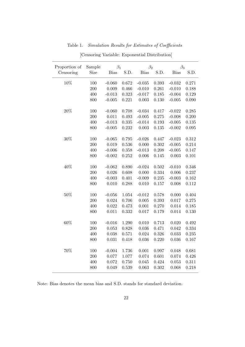
Table 1. Simulation Results for Estimates of Coefficients
[Censoring Variable: Exponential Distribution]
Proportion of Sample β1 β2 β3
Censoring Size Bias S.D. Bias S.D. Bias S.D.
10% 100 -0.060 0.672 -0.035 0.393 -0.032 0.271200 0.009 0.466 -0.010 0.261 -0.010 0.188400 -0.013 0.323 -0.017 0.185 -0.004 0.129800 -0.005 0.221 0.003 0.130 -0.005 0.090
20% 100 -0.060 0.708 -0.034 0.417 -0.022 0.285200 0.011 0.493 -0.005 0.275 -0.008 0.200400 -0.013 0.335 -0.014 0.193 -0.005 0.135800 -0.005 0.232 0.003 0.135 -0.002 0.095
30% 100 -0.065 0.795 -0.026 0.447 -0.023 0.312200 0.019 0.536 0.000 0.302 -0.005 0.214400 -0.006 0.358 -0.013 0.208 -0.005 0.147800 -0.002 0.252 0.006 0.145 0.003 0.101
40% 100 -0.062 0.890 -0.024 0.502 -0.010 0.346200 0.026 0.608 0.000 0.334 0.006 0.237400 -0.003 0.401 -0.009 0.235 -0.003 0.162800 0.010 0.288 0.010 0.157 0.008 0.112
50% 100 -0.056 1.054 -0.012 0.578 0.000 0.404200 0.024 0.706 0.005 0.393 0.017 0.275400 0.022 0.473 0.001 0.270 0.014 0.185800 0.011 0.332 0.017 0.179 0.014 0.130
60% 100 -0.016 1.290 0.010 0.713 0.020 0.492200 0.053 0.828 0.036 0.471 0.042 0.334400 0.038 0.571 0.024 0.326 0.033 0.235800 0.031 0.418 0.036 0.220 0.036 0.167
70% 100 -0.004 1.736 0.001 0.997 0.048 0.681200 0.077 1.077 0.074 0.601 0.074 0.426400 0.072 0.750 0.045 0.424 0.053 0.311800 0.049 0.539 0.063 0.302 0.068 0.218
Note: Bias denotes the mean bias and S.D. stands for standard deviation.
22

Table 2. Simulation Results for Estimates of the Variances
[Censoring Variable: Exponential Distribution]
Proportion of Sample β1 β2 β3
Censoring Size Bias S.D. Bias S.D. Bias S.D.
10% 100 -0.015 0.102 0.002 0.038 0.001 0.018200 -0.015 0.030 0.005 0.011 0.000 0.005400 -0.005 0.010 0.001 0.004 0.001 0.002800 0.000 0.003 0.001 0.001 0.000 0.001
20% 100 0.006 0.130 0.008 0.049 0.006 0.024200 -0.006 0.041 0.010 0.015 0.001 0.007400 0.003 0.013 0.004 0.005 0.002 0.002800 0.003 0.005 0.002 0.002 0.001 0.001
30% 100 -0.001 0.201 0.023 0.069 0.011 0.033200 0.004 0.069 0.013 0.022 0.005 0.011400 0.014 0.022 0.008 0.008 0.004 0.004800 0.007 0.008 0.004 0.003 0.002 0.001
40% 100 0.021 0.332 0.034 0.116 0.021 0.056200 0.006 0.105 0.024 0.037 0.011 0.019400 0.028 0.045 0.012 0.016 0.008 0.008800 0.013 0.017 0.009 0.006 0.005 0.003
50% 100 0.009 0.604 0.058 0.192 0.033 0.103200 0.023 0.191 0.038 0.072 0.020 0.037400 0.044 0.093 0.023 0.032 0.015 0.015800 0.031 0.044 0.018 0.015 0.009 0.007
60% 100 0.009 1.150 0.098 0.502 0.051 0.212200 0.073 0.353 0.061 0.148 0.032 0.081400 0.084 0.176 0.042 0.064 0.022 0.034800 0.046 0.089 0.032 0.035 0.014 0.016
70% 100 0.055 3.859 0.099 1.173 0.055 0.700200 0.079 0.842 0.108 0.321 0.048 0.159400 0.149 0.467 0.084 0.168 0.043 0.097800 0.107 0.250 0.058 0.091 0.030 0.046
Note: Bias denotes the mean bias and S.D. stands for standard deviation. The finite-samplevariances of estimates of coefficients (obtained by 1000 simulations) are treated as the truevalue of the variances.
23

Table 3. Simulation Results for Estimates of Coefficients
[Censoring Variable: Uniform Distribution]
Proportion of Sample β1 β2 β3
Censoring Size Bias S.D. Bias S.D. Bias S.D.
10% 100 -0.057 0.671 -0.032 0.392 -0.029 0.271200 0.013 0.466 -0.009 0.260 -0.009 0.188400 -0.012 0.322 -0.016 0.186 -0.003 0.129800 -0.004 0.222 0.004 0.130 -0.003 0.090
20% 100 -0.046 0.713 -0.024 0.419 -0.012 0.285200 0.028 0.491 0.006 0.273 0.004 0.199400 -0.001 0.338 -0.005 0.193 0.005 0.136800 0.007 0.235 0.011 0.135 0.007 0.095
30% 100 -0.027 0.786 0.012 0.449 0.019 0.313200 0.053 0.543 0.037 0.297 0.037 0.217400 0.034 0.372 0.024 0.210 0.034 0.151800 0.041 0.261 0.040 0.146 0.043 0.103
40% 100 0.034 0.869 0.053 0.498 0.068 0.350200 0.090 0.619 0.084 0.338 0.085 0.242400 0.085 0.421 0.071 0.238 0.085 0.170800 0.089 0.293 0.092 0.166 0.093 0.120
50% 100 0.069 0.994 0.108 0.601 0.137 0.397200 0.160 0.692 0.143 0.394 0.152 0.265400 0.147 0.459 0.139 0.278 0.152 0.187800 0.146 0.342 0.165 0.189 0.155 0.136
60% 100 0.170 1.193 0.192 0.734 0.202 0.471200 0.217 0.803 0.211 0.474 0.224 0.323400 0.232 0.535 0.228 0.321 0.236 0.228800 0.238 0.394 0.245 0.228 0.231 0.161
70% 100 0.259 1.578 0.261 0.899 0.275 0.557200 0.366 0.940 0.344 0.560 0.307 0.379400 0.356 0.647 0.335 0.392 0.324 0.249800 0.326 0.490 0.354 0.281 0.334 0.192
Note: Bias denotes the mean bias and S.D. stands for standard deviation.
24

Table 4. Simulation Results for Estimates of the Variances
[Censoring Variable: Uniform Distribution]
Proportion of Sample β1 β2 β3
Censoring Size Bias S.D. Bias S.D. Bias S.D.
10% 100 -0.013 0.101 0.003 0.037 0.001 0.018200 -0.013 0.031 0.006 0.012 0.000 0.005400 -0.005 0.010 0.001 0.004 0.001 0.002800 0.000 0.004 0.001 0.001 0.000 0.001
20% 100 0.002 0.135 0.006 0.050 0.007 0.024200 -0.003 0.043 0.010 0.015 0.002 0.007400 0.003 0.015 0.005 0.006 0.002 0.003800 0.003 0.006 0.003 0.002 0.001 0.001
30% 100 0.006 0.207 0.019 0.074 0.010 0.036200 0.002 0.096 0.017 0.027 0.005 0.015400 0.011 0.040 0.009 0.013 0.004 0.006800 0.007 0.017 0.005 0.006 0.003 0.003
40% 100 0.016 0.318 0.028 0.116 0.012 0.059200 -0.013 0.138 0.021 0.051 0.008 0.025400 0.013 0.082 0.012 0.030 0.006 0.016800 0.012 0.044 0.008 0.019 0.003 0.008
50% 100 0.005 0.519 -0.002 0.206 0.011 0.082200 -0.005 0.218 0.020 0.097 0.013 0.041400 0.032 0.121 0.011 0.045 0.009 0.025800 0.017 0.100 0.012 0.030 0.006 0.019
60% 100 -0.045 1.178 -0.035 0.499 0.010 0.173200 -0.010 0.358 0.011 0.135 0.008 0.076400 0.033 0.212 0.018 0.097 0.007 0.043800 0.026 0.187 0.013 0.069 0.008 0.044
70% 100 -0.356 2.610 -0.046 0.772 0.028 0.329200 0.009 0.691 0.014 0.244 0.016 0.188400 0.014 0.336 0.011 0.111 0.015 0.058800 0.000 0.258 0.010 0.068 0.006 0.060
Note: Bias denotes the mean bias and S.D. stands for standard deviation. The finite-samplevariances of estimates of coefficients (obtained by 1000 simulations) are treated as the truevalue of the variances.
25