MPRAMunich Personal RePEc Archive

Estimating Recovery Rates on Bank’sHistorical Loan Loss Data

Arindam Bandyopadhyay and Pratima Singh

National Institute of Bank Management (NIBM), Pune

February 2007

Online at http://mpra.ub.uni-muenchen.de/9525/MPRA Paper No. 9525, posted 12. July 2008 14:03 UTC

Estimating Recovery Rates on Bank’s Historical Loan Loss Data*

BY

Arindam Bandyopadhyay (Assistant Professor, NIBM, Email: arindam@nibmindia.org)**

&

Pratima Singh (PGPBF Student, NIBM, Email: pspraty@gmail.com)

* The authors would like to thank Mr. Asit Pal, R. K. Rana and Mr. Ratnesh Mishra for their suggestions and help. ** Corresponding Author-Assistant Professor in Finance, Naitonal Institute of Bank Management, Room No. 3203, Kondhwe Khurd, Pune-411048 India. Tel. 0091-20-26716451.

- 2 –

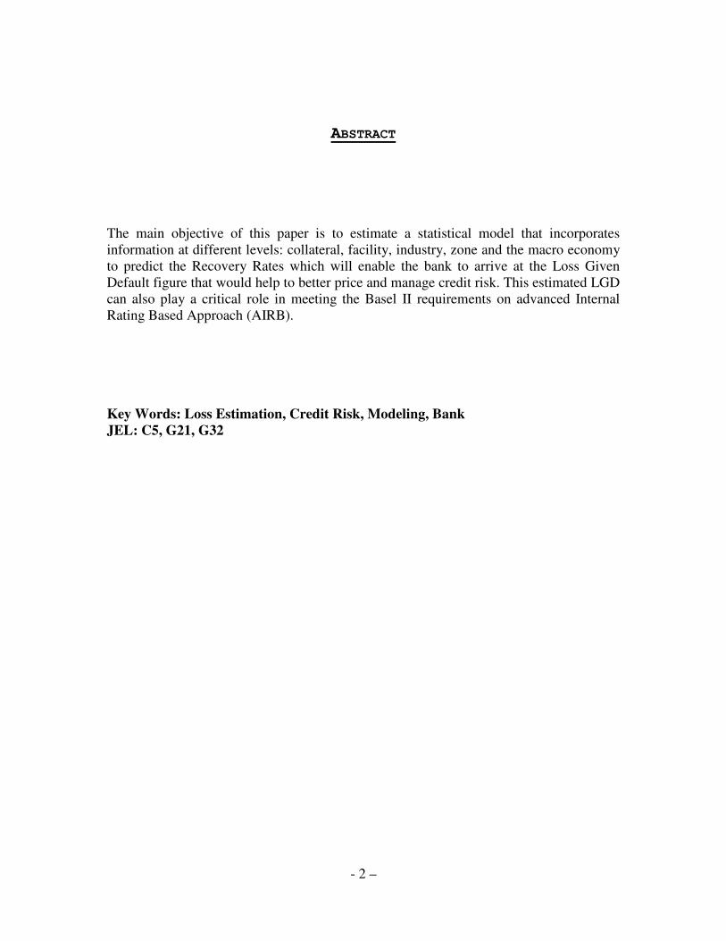
ABSTRACT

The main objective of this paper is to estimate a statistical model that incorporates information at different levels: collateral, facility, industry, zone and the macro economy to predict the Recovery Rates which will enable the bank to arrive at the Loss Given Default figure that would help to better price and manage credit risk. This estimated LGD can also play a critical role in meeting the Basel II requirements on advanced Internal Rating Based Approach (AIRB). Key Words: Loss Estimation, Credit Risk, Modeling, Bank JEL: C5, G21, G32

- 3 –

INTRODUCTION

Loss Given Default is a common parameter in Risk Models and also a parameter used in the calculation of Economic Capital or Regulatory Capital under Basel II for a banking institution. This is an attribute of any exposure on bank's client. If the bank uses the advanced IRB approach, then the Basel II accord allows it to use internal models to estimate LGD. While initially a standard LGD allocation may be used (the foundation Approach), institutions that have adopted the IRB approach for the probability of default are being encouraged to use the IRB approach for the LGD as well since it gives a more accurate assessment of loss. In many cases, this added precision changes capital requirements. In order to quantify for the IRB approach Theoretically, LGD is calculated in different ways, but the most popular is 'Gross' LGD, where total losses are divided by EAD. Another method is to divide Losses by the unsecured portion of a credit line (where security covers a portion of EAD - Exposure at Default). This is known as 'historical' LGD. The historical RR is the sum of the cash flow received from defaulted loans divided by total loan amount due at the time of default (EAD). Economic LGD is the economic loss in the case of default, which can be very different from the accounting one. "Economic" means all costs (direct as well as indirect) incurred with recoveries have to be included in the loss estimate, and that the discounting effects have to be integrated.

MEASURES OF LGD

DEFINITION:

LOSS GIVEN DEFAULT LGD is the fraction of EAD that will not be recovered following default. It is the credit loss incurred if an obligor of the bank defaults

Loss Given Default is facility-specific because such losses are generally understood to be influenced by key transaction characteristics such as the presence of collateral and the degree of subordination.

The loss given default (LGD) is generally defined as

EADamounteryre

LGD_cov

%100 −=

=100% - recovery rate

- 4 –

Loss-given-default (LGD) is an important determinant of credit risk, and is the degree of uncertainty about how much the bank will not be able to collect if a borrower defaults.

Because loan recovery periods may extend over several years, it is necessary to discount post-default net cash flows to a common point in time (the most suitable being the event of default). The LGD on defaulted loan facilities is thus measured by the present value of cash losses with respect to the exposure amount (EAD) at the defaulted year. This can be estimated by calculating the present value of cash received post-default over the year's net discounted cost of recovery.

DETERMINANTS OF RECOVERY/LGD:

Empirically it has been observed that recovery rate (and hence LGD) is dependent on

• The bank’s behavior in terms of debt renegotiation with debtors, compromise and settlements which are country specific.

• The quality of collateral attached to loans

• Firm specific capital structure: Seniority standing of debt in the firm's overall capital structure, leverage etc.

• Industry tangibility: The value of liquidated assets dependent on the industry of the borrower.

• Macro economic factors: industrial production, GDP growth, unemployment rate, interest rate and other macro economic factors have strong influence on LGD.

IMPORTANCE OF LGD:

• LGD is not an issue for the standardized approach. The IRBF approach relies on values furnished by the regulators.

• Institutions planning for the AIRB need to develop methods to estimate LGD, the

credit loss incurred if an obligor of the bank defaults, which is a key component to the credit risk capital or risk weight.

• LGD is an important input for calculation of Expected and Unexpected Credit

Loss and Portfolio Economic Capital.

• According to BIS (June 2006) institutions implementing Advanced-IRB instead of Foundation-IRB will experience larger decreases in Tier 1 capital, and the internal calculation of LGD is a factor separating the two Methods.

- 5 –

• Estimates of LGD are key parameters in a bank's risk-rating system that impact facility ratings, approval levels, and the setting of loss reserves, as well as developing credit capital underlying risk and profitability calculations�

�

�

FOR REGULATORY PURPOSE:

CALCULATING LGD UNDER THE FOUNDATION APPROACH

Under Basel II to calculate the risk-weighted asset, which goes into the determination of the required capital for a bank or financial institution, the institution has to use an estimate of the LGD for each corporate, sovereign and bank exposure. There are two approaches for deriving this estimate: a foundation approach and an advanced approach.

EXPOSURE WITHOUT COLLATERAL

Under the foundation approach, BIS prescribes fixed LGD ratios for certain classes of unsecured exposures:

• Senior claims on corporates, sovereigns and banks not secured by recognized collateral attract a 45% LGD.

• All subordinated claims on corporates, sovereigns and banks attract a 75% LGD.

EXPOSURE WITH COLLATERAL

The effective loss given default (LGD*) applicable to a collateralized transaction can be expressed as

LGD* = LGD x (E* / E)

Where:

LGD is that of the senior unsecured exposure before recognition of collateral (45%).

E is the current value of the exposure (i.e. cash lent or securities lent or posted)

E* should be calculated based on the following formula:

E* = max {0, [E x (1 + He) – C x (1 – Hc – Hfx)]}

Where:

E* = the exposure value after risk mitigation

E = current value of the exposure

- 6 –

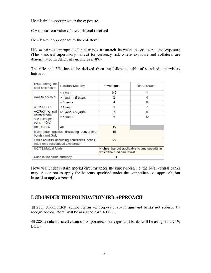
He = haircut appropriate to the exposure

C = the current value of the collateral received

Hc = haircut appropriate to the collateral

Hfx = haircut appropriate for currency mismatch between the collateral and exposure (The standard supervisory haircut for currency risk where exposure and collateral are denominated in different currencies is 8%)

The *He and *Hc has to be derived from the following table of standard supervisory haircuts:

However, under certain special circumstances the supervisors, i.e. the local central banks may choose not to apply the haircuts specified under the comprehensive approach, but instead to apply a zero H.

LGD UNDER THE FOUNDATION IRB APPROACH

¶¶ 287: Under FIRB, senior claims on corporate, sovereigns and banks not secured by recognized collateral will be assigned a 45% LGD.

¶¶ 288: a subordinated claim on corporates, sovereigns and banks will be assigned a 75% LGD.

- 7 –

Collateral under the foundation approach

¶¶ 289: In addition to the eligible financial collateral recognized in the standardized approach, under the FIRB approach some other forms of collateral, known as eligible IRB collateral, are also recognized. These include receivables, specified commercial and residential real estate (CRE/RRE), and other collateral, where they meet the minimum requirements set out in ¶¶ 509-524.

Methodology for determining effective LGD for secured portion:

LGD*=45%-max [0, {min(C/E, C**)-C*}/C**-C*] × (45%-LGDmin)

C**: max & C*: min. |Refer to ¶¶ 295 table

For unsecured portion, ¶¶ 287 & 288 applies

CALCULATING LGD UNDER THE ADVANCED APPROACH

Under the A-IRB approach, the bank itself determines the appropriate Loss given default to be applied to each exposure, on the basis of robust data and analysis. The analysis must be capable of being validated both internally and by supervisors. Thus, a bank using internal Loss Given Default estimates for capital purposes might be able to differentiate Loss Given Default values on the basis of a wider set of transaction characteristics (e.g. product type, wider range of collateral types) as well as borrower characteristics. These values would be expected to represent a conservative view of long-run averages. A bank wishing to use its own estimates of LGD will need to demonstrate to its supervisor that it can meet additional minimum requirements pertinent to the integrity and reliability of these estimates.

DOWNTURN LGD

Under Basel II, banks and other financial institutions are recommended to calculate 'Downturn LGD' (Downturn Loss Given Default), which reflects the losses occurring during a 'Downturn' in a business cycle for regulatory purposes. Downturn LGD is interpreted in many ways, and most financial institutions that are applying for IRB approval under BIS II often have differing definitions of what Downturn conditions are. One definition is at least two consecutive quarters of negative growth in real GDP. Often, negative growth is also accompanied by a negative output gap in an economy (where potential production exceeds actual demand).

The calculation of LGD (or Downturn LGD) poses significant challenges to modelers and practitioners. Final resolutions of defaults can take many years and final losses, and hence final LGD, cannot be calculated until all of this information is ripe. Furthermore, practitioners are of want of data since BIS II implementation is rather new and financial institutions may have only just started collecting the information necessary for calculating the individual elements that LGD is composed of: EAD, direct and indirect Losses, security values and potential, expected future recoveries. Another challenge, and

- 8 –

maybe the most significant, is the fact that the default definitions between institutions vary. This often results in a so-called differing cure-rates or percentage of defaults without losses. Calculation of LGD (average) is often composed of defaults with losses and defaults without. Naturally, when more defaults without losses are added to a sample pool of observations LGD becomes lower. This is often the case when default definitions become more 'sensitive' to credit deterioration or 'early' signs of defaults. When institutions use different definitions, LGD parameters therefore become non-comparable.

Many institutions are scrambling to produce estimates of Downturn LGD, but often resort to 'mapping' since Downturn data is often lacking. Mapping is the process of guestimating losses under a downturn by taking existing LGD and adding a supplement or buffer, which is supposed to represent a potential increase in LGD when Downturn occurs. LGD often decreases for some segments during Downturn since there is a relatively larger increase of defaults that result in higher cure-rates, often the result of temporary credit deterioration that disappears after the Downturn Period is over. Furthermore, LGD values decrease for defaulting financial institutions under economic Downturns because governments and central banks often rescue these institutions in order to maintain financial stability.

APPROACHES FOR LGD ESTIMATES UNDER AIRB APPROCH: Subject to certain additional minimum requirements specified in ¶¶ 468-473, supervisors may permit banks to use their own internal estimates of LGD for corporate, sovereign and bank exposures (and for retail loans also). LGD must be measured as the loss given default as a percentage of the EAD. There might be significant differences in LGD estimation methods across institutions and across portfolios some of which are listed below:

Academic studies provide three kinds of measures to estimate LGDs:

• Market LGD: observed from market prices of defaulted bonds or marketable loans soon after the actual default event. For marketable bonds and loans, the rating agencies attempt to report the trading price of a defaulted obligation one month after default.

• Implied Market LGD: LGDs derived from risky (but not defaulted) bond prices (credit spreads) using a theoretical asset pricing model.

• Workout LGD: This is the observed loss at the end of a workout process when the bank has tried to be paid back and when it decides to close the file.

Market LGD might be an interesting measure, but it has some drawbacks. First, it is limited to listed bonds, that are unsecured most of the time and thus bank cannot draw such figures to compare their loss because bank loans are often backed by various forms of collateral. Secondly, secondary market prices of loans are not available in India

- 9 –

making it practically impossible to use such tools. The implied market LGD approach may be applicable for estimating up to BBB category of corporate assets as bond spreads are not available for non-investment grades (below BBB).

For most bank loans, such market information will not be available, and a bank will have to calculate the economic LGD from its own internal records. This requires discounting of all net cashflows received at an appropriate discount rate. To determine LGD, a bank must be able to identify accurately the borrowers that actually defaulted, the exposures outstanding at the time of default and the amount and timing of repayments ultimately received along with the carrying costs of non-performing loans/facilities (e.g. interest income foregone and workout expenses like collection charges, legal charges, etc.). In addition, demographic information pertaining to the borrower, including industry assignment, public or private designation (constitution) and geographic domicile, are important for developing LGD estimates that are segmented according these characteristics. Finally the structural elements of the defaulted facilities, such as whether the bank’s interest is senior (according to claim: viz. first charge or second charge) or subordinated and whether it has received any collateral, collateral segmentation etc. should be noted.

Ex-post: The ratio of losses post default to the book value of a defaulted obligation after default. Ex-ante: The prediction of losses post default to the predicted Exposure at Default of a non-defaulted obligation.

LGD FIGURES OF BANKS ACROSS GLOBE Moody’s 1970-2003 study of USA bank loans show average LGD rate is 36.1% overall of which corporate LGD rate is as high as 60.09%. Moody’s KMV study (1982-2003) shows in recession, issuer weighted LGD rate for corporate loans peaks up to 67.93% and comes down to 58.61% during expansion. JPMorgan Chase (JPMC) study (2004) shows average discounted LGD on their resolved defaulted loans is 39.8% (discounted at 15%) with standard deviation of 35.4% (for large corporates, LGD is 41.6%). Recently, one International Swaps and Derivatives Association (ISDA) retail portfolio survey (2000) of 14 major financial institutions (like HSBC, ABN Amro, Barclays Bank, Citigroup, Abbey National, Bank One, Deutsche Bank, Allied Irish Bank etc.) from 6 countries shows LGD rates for Mortgages is 20%, on Credit Cards it is 64% and in other retail products is 76%.

Recently, National Institute of Bank Management (NIBM) has proactively undertaken a survey of loss given default of Indian banks to find out the LGD statistics that would help banks to graduate towards IRB approach. Currently, no study on LGD exists for the Indian case from which Indian banks can draw their parallels. Data limitations pose an important challenge to the estimation of LGD internally by banks. Currently, NIBM has collected the loss data on defaulted loans from eight Indian Public Sector Banks (PSBs). Amongst them, two are large, two medium sized and rest are smaller banks. The borrower as well as facility wise recovery information is collected for commercial and retail loans. The preliminary study shows that economic LGD figures for commercial loans are quite higher than the international figures (on average 87% with a standard deviation of 26.8%). The retail loan LGD rate is coming around 74% with standard

- 10 –

deviation of 35.24% which is comparable with the International benchmarks. This may be because of lesser delay in the collection process (2 years on average for retail loans compared to to 4 years in commercial loans). As the time of collection increases, the value of the recovered amount falls and recovery cost (cost of litigation) increases and hence the loss rate goes up. International experiences suggest that the collateral value falls faster than the health of the account. Therefore, it is not enough to know the chance of default of a borrower, but also to understand the collateral cycle and the expected future recovery rate.

Data & Methodology DEFAULT DEFINITION: To study LGD, a definition of default must first be established. This is because historical loss estimates are determined by the definition selected. In this study it is defined as loans that turned NPA according to the standard classification used for bank regulatory reporting. A rich database is compiled that tracks compromised accounts from 2000 to 2007. The compromise proposals in which bank made some future recoveries are mainly included in the database. In case where the compromises failed in making any future recovery or where nothing has been recovered till date, such accounts were not included in the study. DATA: The factors that might affect the recovery rate were identified on the basis of expert judgement and based on the experience of the bank: These factors are as follows:

a) Transaction-related: facility type, collateral type, collateral amount, guarantees, time in default, Loan to value (LTV), date of sanction, date of default, date of compromised, compromised amount, amount write-off, amount waived, recovery till date and recovery procedures.

b) Borrower-related: including borrower size (as it relates to transaction

characteristics), exposure size, firm specific capital structure (as it relates to the firm’s ability to satisfy the claims of its creditors in the event that it defaults), geographic region, industrial sector, and line of business.

c) Institution-related: including internal organization and internal governance,

related events such as mergers, and specific entities within the group dedicated to recoveries such as ‘bad credit institutions’.

d) External: including interest rates and legal framework (and, as a consequence,

the length of the recovery process) and

- 11 –

e) Other risk factors.

Description of the Data, Variables and Summary Statistics

CLASSIFICATION OF FACILITY TYPE: Various credit facilities extended by bank can be classified into two categories viz. fund based and non-fund based. When bank places certain funds at the disposal of borrowers and borrowers avail these funds, such types of credit facilities are known as fund based. However, there are certain types of advances which do not involve deployment of funds at least at the initial stage though in contingencies funds are also involved. These are called non-fund based advances. �

Fund based credit facilities included in the database, used for the study are as following :-��

1. Overdraft 2. Cash-credit 3. Demand loan 4. Term loan 5. Purchasing/Discounting of bills 6. Advanced Bills 7. Packing Credit 8. Foreign Bills Purchased

Non-Fund based facility are as follows:��

1. Letter of Credit 2. Bank Guarantee

Above mentioned all the 10 categories of facility type were considered in the study. Bank did not have facility wise recovery. Hence to calculate Facility-wise LGD for all the facilities taken by the borrower some assumptions were made:

• The amount recovered by the borrower belonged to single facility • Borrowers with multiple facility were allotted single facility type. This was done

by assuming that the borrower had the facility in which he had the highest outstanding balance at the time of default.

• Example: Suppose a borrower had 3 types of facility, lets say Cash credit with 3lacs outstanding at the time of default

Term loan with 1.5 lacs o/s and Bank guarantee with 1.25 lac o/s then in this case, it was considered that the borrower has only cash credit (as it has the highest o/s balance in cash credit).

- 12 –

�

COLLATERAL CLASSIFICATION: The borrowers were segregated on the basis of mode of charging of securities. This was done due to non-availability of complete data relating to the type of collateral available with the bank. Hence the borrowers are segregated on the basis of charge created against the collaterals, as this information was easily available with the bank. �

FOLLOWING ARE THE MODE OF CHARGING THE SECURITIES:

1. Pledge 2. Hypothecation 3. Mortgage

The percentage contribution of borrowers on the basis of different collaterals as follows: maximum number of borrowers had mortgage charge against the collaterals

Collateral wise segregation

1% 14%

12%

49%

21%

2%

1%Mort,Hypo,Pledge

Mortgage &HypothecationHypothecation

Mortgage

Nil

Pledge

Pledge, Mortgage

- 13 –

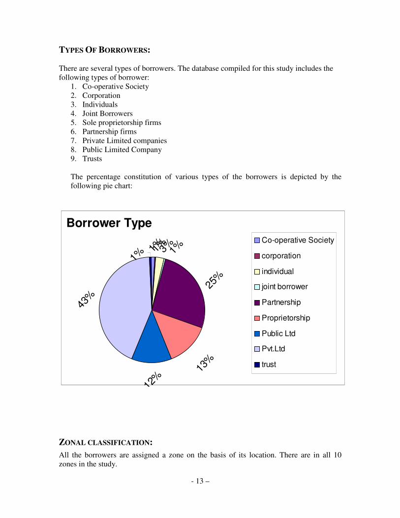
TYPES OF BORROWERS: There are several types of borrowers. The database compiled for this study includes the following types of borrower:

1. Co-operative Society 2. Corporation 3. Individuals 4. Joint Borrowers 5. Sole proprietorship firms 6. Partnership firms 7. Private Limited companies 8. Public Limited Company 9. Trusts The percentage constitution of various types of the borrowers is depicted by the following pie chart:

Borrower Type

1%1%3%1%

25%

13%

12%

43%

1%

Co-operative Society

corporation

individual

joint borrower

Partnership

Proprietorship

Public Ltd

Pvt.Ltd

trust

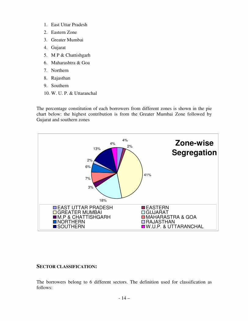
ZONAL CLASSIFICATION: All the borrowers are assigned a zone on the basis of its location. There are in all 10 zones in the study.

- 14 –

1. East Uttar Pradesh

2. Eastern Zone

3. Greater Mumbai

4. Gujarat

5. M P & Chattishgarh

6. Maharashtra & Goa

7. Northern

8. Rajasthan

9. Southern

10. W. U. P. & Uttaranchal

The percentage constitution of each borrowers from different zones is shown in the pie chart below: the highest contribution is from the Greater Mumbai Zone followed by Gujarat and southern zones

Zone-wiseSegregation

4%

41%

18%

3%

7%

6%

2%

13%4%

2%

EAST UTTAR PRADESH EASTERNGREATER MUMBAI GUJARATM.P & CHATTISHGARH MAHARASTRA & GOANORTHERN RAJASTHANSOUTHERN W.U.P. & UTTARANCHAL

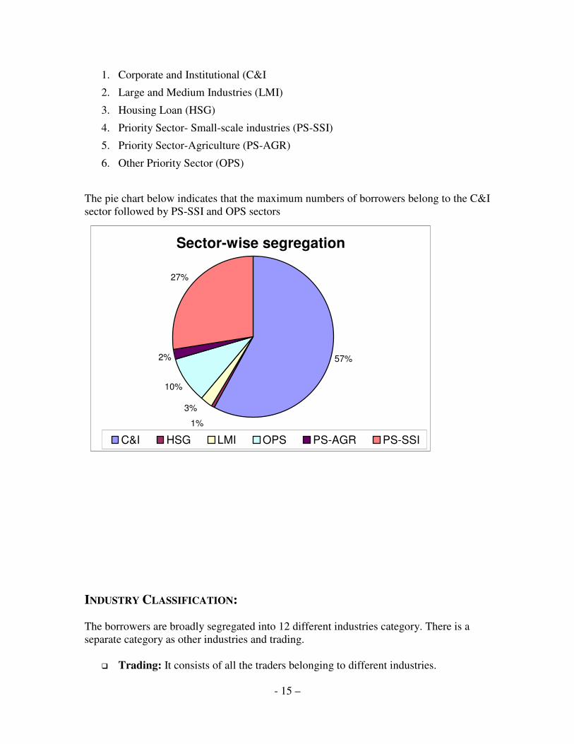
SECTOR CLASSIFICATION: The borrowers belong to 6 different sectors. The definition used for classification as follows:

- 15 –

1. Corporate and Institutional (C&I

2. Large and Medium Industries (LMI)

3. Housing Loan (HSG)

4. Priority Sector- Small-scale industries (PS-SSI)

5. Priority Sector-Agriculture (PS-AGR)

6. Other Priority Sector (OPS)

The pie chart below indicates that the maximum numbers of borrowers belong to the C&I sector followed by PS-SSI and OPS sectors

Sector-wise segregation

57%

1%

3%

10%

2%

27%

C&I HSG LMI OPS PS-AGR PS-SSI

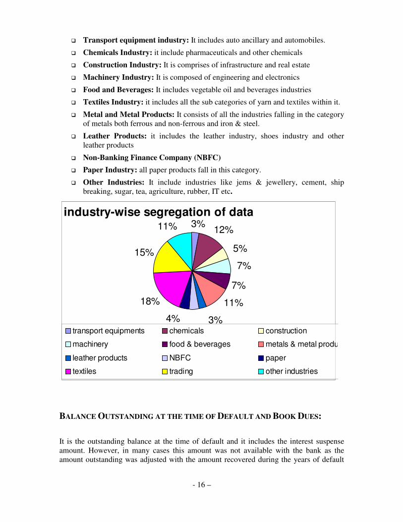
INDUSTRY CLASSIFICATION: The borrowers are broadly segregated into 12 different industries category. There is a separate category as other industries and trading.

� Trading: It consists of all the traders belonging to different industries.

- 16 –

� Transport equipment industry: It includes auto ancillary and automobiles.

� Chemicals Industry: it include pharmaceuticals and other chemicals

� Construction Industry: It is comprises of infrastructure and real estate

� Machinery Industry: It is composed of engineering and electronics

� Food and Beverages: It includes vegetable oil and beverages industries

� Textiles Industry: it includes all the sub categories of yarn and textiles within it.

� Metal and Metal Products: It consists of all the industries falling in the category of metals both ferrous and non-ferrous and iron & steel.

� Leather Products: it includes the leather industry, shoes industry and other leather products

� Non-Banking Finance Company (NBFC) � Paper Industry: all paper products fall in this category.

� Other Industries: It include industries like jems & jewellery, cement, ship breaking, sugar, tea, agriculture, rubber, IT etc.

industry-wise segregation of data3% 12%

5%

7%

7%

11%

3%

4%

4%

18%

15%

11%

transport equipments chemicals construction

machinery food & beverages metals & metal products

leather products NBFC paper

textiles trading other industries

BALANCE OUTSTANDING AT THE TIME OF DEFAULT AND BOOK DUES:

It is the outstanding balance at the time of default and it includes the interest suspense amount. However, in many cases this amount was not available with the bank as the amount outstanding was adjusted with the amount recovered during the years of default

- 17 –

(period between the date of default and date of compromise) thus reducing it by the recovered amount.

Book dues are outstanding less interest suspense. The similar problem persists with the book dues, which makes it lesser than what it should have been.

Hence, while estimating LGD, book dues plus unapplied interest are considered for calculating the Exposure at Default (EAD). However, ideally balance outstanding at the tine of default is the EAD.

CONTRACTUAL LENDING RATES: In practice, since loan-specific contractual lending rates were not often available for the study, a more generic set of interest rates were used, namely, the the last three years average PLR rates.

DATE OF DEFAULT: It the date on which the loan account turned NPA according to the standard classification used for bank regulatory reporting.

DATE OF SANCTION: It is the date on which the loan facility was sanctioned to the borrower. In this study the range of date of sanction of loan facility is 1953-2001

DATE OF COMPROMISE: It is the date on which the defaulted loan was sanctioned for the compromise by the bank. The compromises made at BCC level, PSR (Mumbai) and zonal level between 2001-2007 are included in the study.

YEARS IN DEFAULT: It is the time period between the date of NPA and date of compromise of the proposal.

AGE OF LOAN: It is the period between date of sanction of loan amount and date of sanction for compromise by the bank. RECOVERY COST: It includes expenses incurred in recovering the amount due from the borrower. Mainly it includes the legal charges incurred by the bank in recovering the dues.

- 18 –

FINANCIALS OF THE BORROWER: Since the borrower-specific data about the financials of the borrower was not recorded by the bank. Last five years industry average figure was used as a proxy for the borrower financial data e.g. Current Ratio, Quick Ratio, Debt-Equity Ratio, Solvency Ratio, Profits, Total assets etc.

METHODOLOGY

Data was collected as per a format having information related to the above mentioned variables categories and other factors like IIP, contractual lending rates etc. Based on the data the LGD was calculated in three ways: 1) HISTORICAL LGD: This is a simply 1- recovery rate. The recovery till date had been reduced by the recovery cost. This amount was used in the numerator. This was divided by the EAD (denominator). This gave the recovery rates. 2) ECONOMIC LGD (DISCOUNTED CASHFLOW LGD): The amount recovered till date was reduced by the recovery cost. This amount was discounted @11.16% for the number of years in default. This gave the discounted recovery. It was then divided by EAD (denominator). This rate is the recovery rate. The recovery was flatly discounted by a single rate of discount. This was done because the data on the year-wise recovery and the rate of discount was not available. Hence, this figure obtained by discounting at the flat rate of 11.16% is an approximation. The actual could not be calculated. 3) PREDICTED LGD: It was seen that, in few cases, the Recovery Rates calculated by the above mentioned method were negative) and had non-normal distribution so a better method was used to predict the LGD. This was done with the help of tobit regression modeling. This takes care of non-linearity if any because it uses maximum likelihood method which is much better than the ordinary lease square. Moreover, since Recovery rates should typically varies from 0-100 percent, Tobit censored regression was considered to be appropriate statistical technique to estimate the recovery rate. Tobit regression exercise was done in statistical package STATA 9.

- 19 –

This exercise was done by keeping the Recovery rates as the dependent variable. Regression was run on the independent variables. At first, based on the expert judgement, some parameters like size of exposure, age of loan, number of years in default, industry etc were used to estimate the regression equation. Then significance of each independent variable was tested. If a particular variable in the estimated regression equation was insignificant then the same exercise was re-run, taking other variables in the regression equation. This was done till all the variables in the regressed equation very significant with correct signs. This gave the final regression equation. After the estimation, the estimated coefficients of the parameters were multiplied by the values of the explanatory variables and added together along with the intercept, this is the predicted Recovery rate. The LGD of the loan will be 1 minus recovery rate. Predicted LGD = 1- Predicted Recovery Rates.

RESULTS ANALYSIS AND INTERPRETATION THE RESULTS ARE AS FOLLOWS: The simple average LGD for the bank: No. of Borrowers Historical LGD Eco LGD Predicted LGD

Mean 64.65% 82.14% 64.77% 200 Stdev 23.76% 17.22% 12.92% The weighted average LGD for the bank, taking exposure at default as weights: EAD weighted average historical LGD for the bank: 68.32% EAD weighted average Economic LGD: 83.9% The EAD weighted average predicted LGD: 70.29% While normally bank can take 70.29% as average LGD and in worst condition, it would be 83.9% On running the regression exercise as mention in methodology for the predicted LGD, the following model was estimated. This is perhaps the best model that was estimated with the available data. All the variables have expected signs. There are some variables like, the loan size which has the expected sign but it is insignificant. Inspite of it being insignificant, it is included in the model because it is included as control variable. Control variables are those variables which are important for the dependent variable and whose effect has to be incorporated in the same. Similarly the industry dummies, specific Collateral dummies and zone dummies are insignificant but included in the model, since they are control variables. All other variables in the model like, the facility type code, collateral dummy, number of years in default, age of loan and loan to value ratio are significant and have expected signs. The model test indicated by LR chi2 (32) shows that it fits very well. LR Chi2 (32) is 67.56, it is like F test of significance. Pseudo R2 is not like R2 but it also shows very high. However in case of tobit regression it does not have much meaning. So it can be

- 20 –

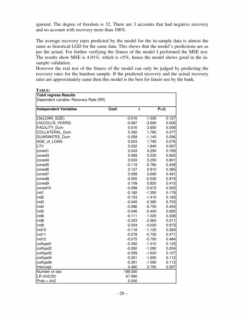
ignored. The degree of freedom is 32. There are 3 accounts that had negative recovery and no account with recovery more than 100%. The average recovery rates predicted by the model for the in-sample data is almost the same as historical LGD for the same data. This shows that the model’s predictions are as per the actual. For further verifying the fitness of the model I performed the MSE test. The results show MSE is 4.01%, which is <5%, hence the model shows good in the in-sample validation. However the real test of the fitness of the model can only be judged by predicting the recovery rates for the handout sample. If the predicted recovery and the actual recovery rates are approximately same then this model is the best for future use by the bank. TABLE: Tobit regress ResultsDependent variable: Recovery Rate (RR)

Independent Variables Coef. t P>|t|

LN(LOAN_SIZE) -0.016 -1.530 0.127LN(COLLN_YEARS) -0.087 -3.690 0.000FACILITY_Dum 0.016 2.650 0.009COLLATERAL_Dum 0.392 1.780 0.077GUARANTEE_Dum -0.058 -1.140 0.256AGE_of_LOAN 0.003 1.790 0.076LTV 0.022 1.840 0.067zoned1 0.043 0.290 0.769zoned3 0.069 0.530 0.600zoned4 0.033 0.250 0.801zoned5 -0.119 -0.780 0.439zoned6 0.127 0.910 0.365zoned7 0.099 0.690 0.491zoned8 -0.005 -0.030 0.974zoned9 0.109 0.820 0.415zoned10 -0.099 -0.670 0.505ind1 -0.182 -1.350 0.179ind2 -0.153 -1.410 0.160ind3 -0.045 -0.380 0.703ind4 -0.086 -0.750 0.453ind5 -0.046 -0.400 0.692ind6 -0.111 -1.020 0.308ind8 -0.323 -2.560 0.011ind9 -0.004 -0.030 0.973ind10 -0.118 -1.120 0.264ind11 -0.078 -0.720 0.471ind12 -0.075 -0.700 0.484colltypd1 -0.392 -1.510 0.133colltypd2 -0.282 -1.280 0.204colltypd3 -0.359 -1.620 0.107colltypd4 -0.351 -1.600 0.112colltypd6 -0.391 -1.590 0.113Intercept 0.480 2.750 0.007Number of obs 199.000LR chi2(32) 67.560Prob > chi2 0.000

- 21 –

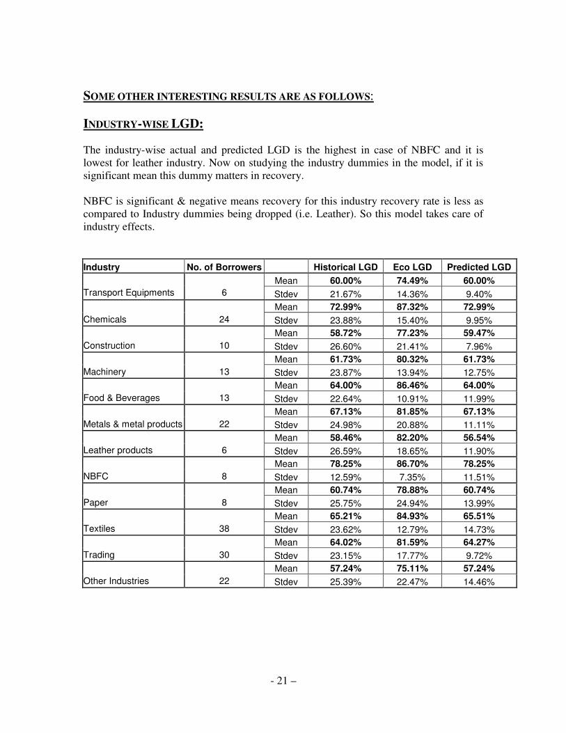
SOME OTHER INTERESTING RESULTS ARE AS FOLLOWS: INDUSTRY-WISE LGD: The industry-wise actual and predicted LGD is the highest in case of NBFC and it is lowest for leather industry. Now on studying the industry dummies in the model, if it is significant mean this dummy matters in recovery. NBFC is significant & negative means recovery for this industry recovery rate is less as compared to Industry dummies being dropped (i.e. Leather). So this model takes care of industry effects. Industry No. of Borrowers Historical LGD Eco LGD Predicted LGD

Mean 60.00% 74.49% 60.00% Transport Equipments 6 Stdev 21.67% 14.36% 9.40%

Mean 72.99% 87.32% 72.99% Chemicals 24 Stdev 23.88% 15.40% 9.95%

Mean 58.72% 77.23% 59.47% Construction 10 Stdev 26.60% 21.41% 7.96%

Mean 61.73% 80.32% 61.73% Machinery 13 Stdev 23.87% 13.94% 12.75%

Mean 64.00% 86.46% 64.00% Food & Beverages 13 Stdev 22.64% 10.91% 11.99%

Mean 67.13% 81.85% 67.13% Metals & metal products 22 Stdev 24.98% 20.88% 11.11%

Mean 58.46% 82.20% 56.54% Leather products 6 Stdev 26.59% 18.65% 11.90%

Mean 78.25% 86.70% 78.25% NBFC 8 Stdev 12.59% 7.35% 11.51%

Mean 60.74% 78.88% 60.74% Paper 8 Stdev 25.75% 24.94% 13.99%

Mean 65.21% 84.93% 65.51% Textiles 38 Stdev 23.62% 12.79% 14.73%

Mean 64.02% 81.59% 64.27% Trading 30 Stdev 23.15% 17.77% 9.72%

Mean 57.24% 75.11% 57.24% Other Industries 22 Stdev 25.39% 22.47% 14.46%

- 22 –

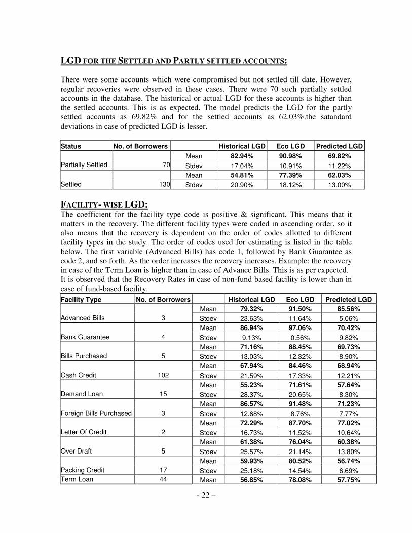
LGD FOR THE SETTLED AND PARTLY SETTLED ACCOUNTS: There were some accounts which were compromised but not settled till date. However, regular recoveries were observed in these cases. There were 70 such partially settled accounts in the database. The historical or actual LGD for these accounts is higher than the settled accounts. This is as expected. The model predicts the LGD for the partly settled accounts as 69.82% and for the settled accounts as 62.03%.the satandard deviations in case of predicted LGD is lesser. Status No. of Borrowers Historical LGD Eco LGD Predicted LGD

Mean 82.94% 90.98% 69.82% Partially Settled 70 Stdev 17.04% 10.91% 11.22%

Mean 54.81% 77.39% 62.03% Settled 130 Stdev 20.90% 18.12% 13.00% FACILITY- WISE LGD: The coefficient for the facility type code is positive & significant. This means that it matters in the recovery. The different facility types were coded in ascending order, so it also means that the recovery is dependent on the order of codes allotted to different facility types in the study. The order of codes used for estimating is listed in the table below. The first variable (Advanced Bills) has code 1, followed by Bank Guarantee as code 2, and so forth. As the order increases the recovery increases. Example: the recovery in case of the Term Loan is higher than in case of Advance Bills. This is as per expected. It is observed that the Recovery Rates in case of non-fund based facility is lower than in case of fund-based facility. Facility Type No. of Borrowers Historical LGD Eco LGD Predicted LGD

Mean 79.32% 91.50% 85.56% Advanced Bills 3 Stdev 23.63% 11.64% 5.06%

Mean 86.94% 97.06% 70.42% Bank Guarantee 4 Stdev 9.13% 0.56% 9.82%

Mean 71.16% 88.45% 69.73% Bills Purchased 5 Stdev 13.03% 12.32% 8.90%

Mean 67.94% 84.46% 68.94% Cash Credit 102 Stdev 21.59% 17.33% 12.21%

Mean 55.23% 71.61% 57.64% Demand Loan 15 Stdev 28.37% 20.65% 8.30%

Mean 86.57% 91.48% 71.23% Foreign Bills Purchased 3 Stdev 12.68% 8.76% 7.77%

Mean 72.29% 87.70% 77.02% Letter Of Credit 2 Stdev 16.73% 11.52% 10.64%

Mean 61.38% 76.04% 60.38% Over Draft 5 Stdev 25.57% 21.14% 13.80%

Mean 59.93% 80.52% 56.74% Packing Credit 17 Stdev 25.18% 14.54% 6.69% Term Loan 44 Mean 56.85% 78.08% 57.75%

- 23 –

Stdev 25.83% 16.35% 12.74%

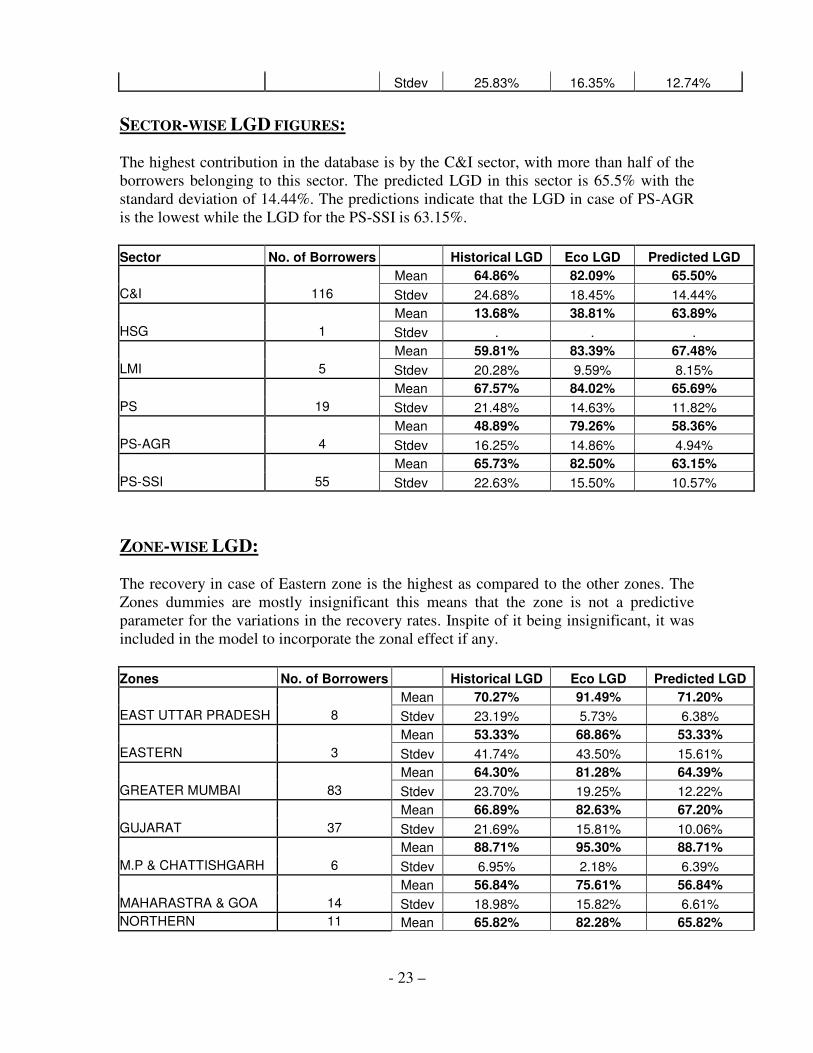
SECTOR-WISE LGD FIGURES: The highest contribution in the database is by the C&I sector, with more than half of the borrowers belonging to this sector. The predicted LGD in this sector is 65.5% with the standard deviation of 14.44%. The predictions indicate that the LGD in case of PS-AGR is the lowest while the LGD for the PS-SSI is 63.15%. Sector No. of Borrowers Historical LGD Eco LGD Predicted LGD

Mean 64.86% 82.09% 65.50% C&I 116 Stdev 24.68% 18.45% 14.44%

Mean 13.68% 38.81% 63.89% HSG 1 Stdev . . .

Mean 59.81% 83.39% 67.48% LMI 5 Stdev 20.28% 9.59% 8.15%

Mean 67.57% 84.02% 65.69% PS 19 Stdev 21.48% 14.63% 11.82%

Mean 48.89% 79.26% 58.36% PS-AGR 4 Stdev 16.25% 14.86% 4.94%

Mean 65.73% 82.50% 63.15% PS-SSI 55 Stdev 22.63% 15.50% 10.57%

ZONE-WISE LGD: The recovery in case of Eastern zone is the highest as compared to the other zones. The Zones dummies are mostly insignificant this means that the zone is not a predictive parameter for the variations in the recovery rates. Inspite of it being insignificant, it was included in the model to incorporate the zonal effect if any. Zones No. of Borrowers Historical LGD Eco LGD Predicted LGD

Mean 70.27% 91.49% 71.20% EAST UTTAR PRADESH 8 Stdev 23.19% 5.73% 6.38%

Mean 53.33% 68.86% 53.33% EASTERN 3 Stdev 41.74% 43.50% 15.61%

Mean 64.30% 81.28% 64.39% GREATER MUMBAI 83 Stdev 23.70% 19.25% 12.22%

Mean 66.89% 82.63% 67.20% GUJARAT 37 Stdev 21.69% 15.81% 10.06%

Mean 88.71% 95.30% 88.71% M.P & CHATTISHGARH 6 Stdev 6.95% 2.18% 6.39%

Mean 56.84% 75.61% 56.84% MAHARASTRA & GOA 14 Stdev 18.98% 15.82% 6.61% NORTHERN 11 Mean 65.82% 82.28% 65.82%

- 24 –

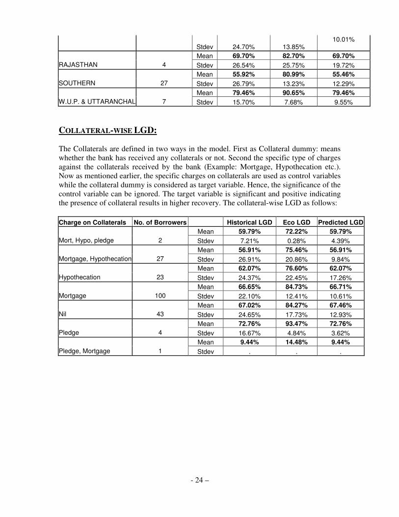
Stdev 24.70% 13.85% 10.01%

Mean 69.70% 82.70% 69.70%

RAJASTHAN 4 Stdev 26.54% 25.75% 19.72% Mean 55.92% 80.99% 55.46%

SOUTHERN 27 Stdev 26.79% 13.23% 12.29% Mean 79.46% 90.65% 79.46%

W.U.P. & UTTARANCHAL 7 Stdev 15.70% 7.68% 9.55% COLLATERAL-WISE LGD: The Collaterals are defined in two ways in the model. First as Collateral dummy: means whether the bank has received any collaterals or not. Second the specific type of charges against the collaterals received by the bank (Example: Mortgage, Hypothecation etc.). Now as mentioned earlier, the specific charges on collaterals are used as control variables while the collateral dummy is considered as target variable. Hence, the significance of the control variable can be ignored. The target variable is significant and positive indicating the presence of collateral results in higher recovery. The collateral-wise LGD as follows: Charge on Collaterals No. of Borrowers Historical LGD Eco LGD Predicted LGD

Mean 59.79% 72.22% 59.79% Mort, Hypo, pledge 2 Stdev 7.21% 0.28% 4.39%

Mean 56.91% 75.46% 56.91% Mortgage, Hypothecation 27 Stdev 26.91% 20.86% 9.84%

Mean 62.07% 76.60% 62.07% Hypothecation 23 Stdev 24.37% 22.45% 17.26%

Mean 66.65% 84.73% 66.71% Mortgage 100 Stdev 22.10% 12.41% 10.61%

Mean 67.02% 84.27% 67.46% Nil 43 Stdev 24.65% 17.73% 12.93%

Mean 72.76% 93.47% 72.76% Pledge 4 Stdev 16.67% 4.84% 3.62%

Mean 9.44% 14.48% 9.44% Pledge, Mortgage 1 Stdev . . .

- 25 –

CONCLUSIONS & RECOMMENDATIONS

IMPORTANCE OF THE MODEL This model can be used by the bank for predicting the future recovery rates of their standard accounts or new accounts. For this the Bank needs all the above variable information that has been used in the tobit recovery model. The coefficients & variable values are multiplied correspondally and finally added together to get a predicted recovery rate. The recovery rates thus estimated should be discounted by appropriate rate of discount. Example: Predicted recovery rate for next 1 year =predicted RR *exp (-rate of discount*1) For next two years (anticipated recovery) = predicted RR *exp (-rate of discount*2) DIFFICULTIES & SUGGESTIONS:

• First, data limitations pose an important challenge to the estimation of LGD parameters in general, and of LGD parameters consistent with economic downturn conditions in particular. Hence we suggest, that bank should have a systematic method of recording the data.

• Second, Due to the non-availability of some of the important data with the bank

like year-wise recovery, amount outstanding at the time of default etc., some assumptions were used (explained in the detailed description of the data). This has led to the lower accuracy in the estimation of the LGD.

• Third, the bank needs to have some people who are especially involved in the

process of collecting the required data for the future studies. The appropriate data is the backbone of any statistical study.

• Fourth, had there been enough data, the model would have given better results.

Therefore, we suggest bank to recalibrate the model with bigger sample data and validate it with a handout sample before putting it to use.

• Sixth, Since LGD estimation is the dynamic process, we suggest the bank to use

the following format in the compromise proposal so that it is easier to collect the data for the further improvement and recalibration of the tobit recovery model estimated in this study

- 26 –

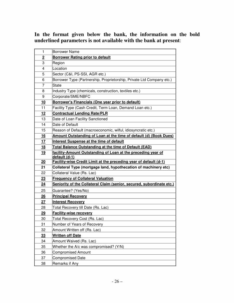
In the format given below the bank, the information on the bold underlined parameters is not available with the bank at present:

1 Borrower Name 2 Borrower Rating prior to default 3 Region 4 Location 5 Sector (C&I, PS-SSI, AGR etc.) 6 Borrower Type (Partnership, Proprietorship, Private Ltd Company etc.) 7 State 8 Industry Type (chemicals, construction, textiles etc.) 9 Corporate/SME/NBFC 10 Borrower's Financials (One year prior to default) 11 Facility Type (Cash Credit, Term Loan, Demand Loan etc.) 12 Contractual Lending Rate/PLR 13 Date of Loan Facility Sanctioned 14 Date of Default 15 Reason of Default (macroeconomic, wilful, idiosyncratic etc.) 16 Amount Outstanding of Loan at the time of default (d) (Book Dues) 17 Interest Suspense at the time of default 18 Total Balance Outstanding at the time of Default (EAD) 19 facility-Amount Outstanding of Loan at the preceding year of

default (d-1) 20 Facility-wise Credit Limit at the preceding year of default (d-1) 21 Collateral Type (mortgage land, hypothecation of machinery etc) 22 Collateral Value (Rs. Lac) 23 Frequency of Collateral Valuation 24 Seniority of the Collateral Claim (senior, secured, subordinate etc.)

25 Guarantee? (Yes/No) 26 Principal Recovery 27 Interest Recovery 28 Total Recovery till Date (Rs. Lac) 29 Facility-wise recovery 30 Total Recovery Cost (Rs. Lac) 31 Number of Years of Recovery 32 Amount Written off (Rs. Lac) 33 Written off Date 34 Amount Waived (Rs. Lac) 35 Whether the A/c was compromised? (Y/N) 36 Compromised Amount 37 Compromised Date 38 Remarks if Any

- 27 –

RECOMMENDATIONS FOR FUTURE STUDY: This study can be further extended to rate the borrower through a LGD rating model. Bank can rate the borrower on the basis of the predicted recovery rates, which the model will estimate. Based on this estimation benchmarking can be done for different category of borrowers. The borrower with the highest recovery rates will be given AAA grade. Similarly grades can be benchmarked for the lower grades. Thus the facility rating and the borrower rating can be clubbed together, if the bank uses the LGD rating Model. However before carrying forward the exercise the model should be validated with handout sample. Moreover bank need to have the rating information of the borrower.

SUMMARY & CONCLUSIONS Building a Recovery Model from loss perspective is hard. This is because it is difficult to get enough predictive data since there are few commercial defaults. Therefore, the time needed to collect default data was substantial. Total default data used in estimating the recovery model was of 200 defaulted borrowers. There are different approaches to calculate LGD. In this project, on the basis of data available for study, I’ve calculated it in three ways, namely the historical or accounting LGD, Economic LGD and Predicted LGD. The historical LGD is the calculated by directly dividing the net recovery till date with the EAD, the economic LGD was calculated by discounting the net recovery till date, at the rate of last three years average PLR. The predicted LGD calculated on the basis of a recovery model estimated with the given data. The recovery model can predict the LGD for the standard accounts s well. Hence it will be useful for the bank in estimating the future recovery rates for these accounts. Some interesting results were as follows: The weighted average actual LGD for the bank studied in this paper is 68.32%. The model predicts the LGD to be 70.29%. In worst conditions the economic LGD is 83.9%. On further analysis it was found that the services industry had higher LGD compared to the manufacturing or trading industry. Facility-wise analysis shows that the bank has higher recovery rates in case of fund-based facility than in case of non-fund based sanctions. The defaulted accounts that were compromised and settled had lower LGD than the accounts that were compromised and partly settled (recovery was in progress). The sector-wise analysis indicated that the highest rate of recovery was in the PS-AGR sector followed by the PS-SSI sector, while the lowest recovery was fro the LMI sector.

- 28 –

The recovery model estimated in this project work has been validated with in-sample testing. However, the bank should use this model only after validating it with handout sample. The validation with handout sample was not in the scope of this study.

REFERENCES

� Altman, E. I., and V. Kishore, 1996 (November-December), “Almost Everything You wanted to Know about Recoveries on Defaulted Bonds,” Financial Analysts Journal, pp. 57-64.

� Altman, E. I., D. Crooke, and V. Kishore, 1999, “Defaults and Returns on High-Yield Bonds: Analysis through 1998 and Default Outlook for 1998-2001, “ Working Paper, New York University Salomon Center, January.

� Altman, E. I., et al, 2005, “The Link between Default and Recovery Rates: Theory, Empirical Evidence, and Implications”, Journal of Business, November.

� Araten, M., M. Jacobs Jr, and P. Varshney, 2004, “Measuring LGD on Commercial Loans: An 18-Year Internal Study”, RMA Journal, May.

� Bandyopadhyay, A., 2007, A note on Measurement and Management of Credit Risk under Basel II, NIBM, monograph, pp. 44-61.

� ______________, 2007, Poor default history, Business Standard, 27th December, pp. 10.

� Basel II: International Convergence of Capital Measurement and Capital Standards: a Revised Framework, Comprehensive Version (BCBS) (June 2006 Revision)

� De Servigny, A., and O. Renault, 2004, Measuring and Managing Credit Risk, Standard & Poor’s, McGraw-Hill.

� Izvorski, I., 1997, “Recovery Ratios and Survival Times for Corporate Bonds,” Working Paper, IMF.

� Morrison, J. S., 2003 (May), “Preparing for Basel II Modeling Requirements. Part 1: Model Development”, RMA Journal, pp. 56-61.

� Schuermann, T., 2004, “What Do We Know About Loss Given Default?”, Working Paper, Wharton, Federal Reserve Bank of New York.

� The Basel Handbook: A Guide for Financial Practitioners, 2nd Edition, Edited by Michael Ong, Riskbooks, 2007.

� Yawitz, J. B., 1977, “An Analytical Model of Interest Rate Differentials and Different Default Recoveries,” Journal of Financial and Quantitative Analysis, Vol. 13, pp. 481-490.

� Asarnow, Elliot, and David Edwards. "Measuring Loss on Defaulted Bank Loans: A 24-Year Study", Journal of Commercial Lending, (Mar-1995), Vol. 77, No.7, pp. 11-23.