Estimating surface CO ﬂuxes from space-borne CO dry air ... · PDF filelar Occultation FTS for Inclined-Orbit Satellite sensor for sur-face source inversion, J. Geophys. Res., 108(D24),

Atmos. Chem. Phys., 9, 2619–2633, 2009www.atmos-chem-phys.net/9/2619/2009/© Author(s) 2009. This work is distributed underthe Creative Commons Attribution 3.0 License.

AtmosphericChemistry

and Physics

Estimating surface CO2 fluxes from space-borne CO2 dry air molefraction observations using an ensemble Kalman Filter

L. Feng1, P. I. Palmer1, H. Bosch2, and S. Dance3

1School of GeoSciences, University of Edinburgh, King’s Buildings, Edinburgh EH9 3JN, UK2Department of Physics and Astronomy, University of Leicester, Leicester LE1 7RH, UK3Department of Mathematics and Department of Meteorology, University of Reading, Reading RG6 6BB, UK

Received: 8 September 2008 – Published in Atmos. Chem. Phys. Discuss.: 28 November 2008Revised: 2 April 2009 – Accepted: 2 April 2009 – Published: 15 April 2009

Abstract. We have developed an ensemble Kalman Filter(EnKF) to estimate 8-day regional surface fluxes of CO2from space-borne CO2 dry-air mole fraction observations(XCO2) and evaluate the approach using a series of syntheticexperiments, in preparation for data from the NASA OrbitingCarbon Observatory (OCO). The 32-day duty cycle of OCOalternates every 16 days between nadir and glint measure-ments of backscattered solar radiation at short-wave infraredwavelengths. The EnKF uses an ensemble of states to rep-resent the error covariances to estimate 8-day CO2 surfacefluxes over 144 geographical regions. We use a 12×8-day lagwindow, recognising that XCO2 measurements include sur-face flux information from prior time windows. The obser-vation operator that relates surface CO2 fluxes to atmosphericdistributions of XCO2 includes: a) the GEOS-Chem transportmodel that relates surface fluxes to global 3-D distributionsof CO2 concentrations, which are sampled at the time andlocation of OCO measurements that are cloud-free and haveaerosol optical depths<0.3; and b) scene-dependent aver-aging kernels that relate the CO2 profiles to XCO2, account-ing for differences between nadir and glint measurements,and the associated scene-dependent observation errors. Weshow that OCO XCO2 measurements significantly reduce theuncertainties of surface CO2 flux estimates. Glint measure-ments are generally better at constraining ocean CO2 flux es-timates. Nadir XCO2 measurements over the terrestrial trop-ics are sparse throughout the year because of either clouds orsmoke. Glint measurements provide the most effective con-straint for estimating tropical terrestrial CO2 fluxes by accu-rately sampling fresh continental outflow over neighbouringoceans. We also present results from sensitivity experimentsthat investigate how flux estimates change with 1) bias and

Correspondence to:L. Feng([email protected])

unbiased errors, 2) alternative duty cycles, 3) measurementdensity and correlations, 4) the spatial resolution of estimatedflux estimates, and 5) reducing the length of the lag windowand the size of the ensemble. At the revision stage of thismanuscript, the OCO instrument failed to reach its orbit afterit was launched on 24 February 2009. The EnKF formulationpresented here is also applicable to GOSAT measurements ofCO2 and CH4.

1 Introduction

CO2 surface fluxes inferred from atmospheric CO2 con-centrations by inverting models of atmospheric transporthave led to substantial improvements in our understandingof the contemporary carbon cycle (e.g.,Bousquet et al.,2000). Previous studies that employ these methods to es-timate surface fluxes of CO2 have tended to use accurate,but spatially sparse and heterogeneous, ground-based mea-surements, which were not designed for the flux estimationproblem, consequently limiting the extent of spatial disag-gregation of fluxes that can be achieved (e.g.,Houwelinget al., 1999; Rodenbeck et al., 2003). Satellite measurementsof CO2 offer new constraints for estimating surface fluxes.The SCanning Imaging Absorption spectroMeter for Atmo-spheric ChartograpHY (SCIAMACHY) satellite instrument(Bovensmann et al., 1999) has measured short-wave infra-red wavelengths (SWIR), with greatest sensitivity to CO2 inthe lower troposphere, since its launch in 2002. Current CO2column volume mixing ratio products from SCIAMACHYhave an estimated measurement accuracy of between 1 and5% (Schneising et al., 2008; Barkley et al., 2006, 2007). Un-characterized systematic and random errors (e.g.,Houwelinget al., 2005), while the subject of ongoing research (Schneis-ing et al., 2008), limit the application of these data for surface

Published by Copernicus Publications on behalf of the European Geosciences Union.

http://creativecommons.org/licenses/by/3.0/

2620 L. Feng et al.: Estimating surface flux

flux estimation. Top-down studies that use satellite mea-surements of CO2 retrieved at thermal infra-red wavelengths,with greatest vertical sensitivity in the free troposphere, haveconcluded that uncharacterized observation and model bi-ases compromise resulting surface flux estimates (Chevallieret al., 2005; Tiwari et al., 2006).

The NASA Orbiting Carbon Observatory (OCO)1 (Crispet al., 2004), and Japanese Greenhouse Observing SATellite(GOSAT) (Maksyutov et al., 2008), launched in early 2009,measure SWIR wavelengths, that are sensitive to CO2 in thefree and lower troposphere. OCO and GOSAT will operatetwo modes of observation: (1) nadir, and (2) glint, wherethe instrument boresight is directed off-nadir to the angle ofspecular reflection. The glint mode increases the signal tonoise of measurements over the ocean. Dry-air CO2 molefractions (XCO2) will be retrieved from the observed spec-tra to a precision of 1–2 ppmv (parts per million by volume)(Crisp et al., 2004), a level of precision necessary to im-prove upon constraints from existing in situ measurements(Rayner et al., 2002; Patra et al., 2003; Miller et al., 2007).We focus on OCO measurements of CO2, but the generalassimilation approach described here can easily be appliedto GOSAT measurements of CO2 or CH4. Recent studieshave used variational data assimilation methods with syn-thetic OCO observations to show that these data have thepotential to estimate weekly and daily surface CO2 fluxes atmodel grid scales of order 3.75◦ in longitude and 2.5◦ in lat-itude (Baker et al., 2006; Chevallier et al., 2007a; Chevallier,2007b). These studies (1) assumed a constant measurementerror (1–2 ppmv), and (2) used a flat weighting function toconvert the model vertical CO2 profiles into XCO2.

We have developed an Ensemble Kalman Filter (EnKF)(Evensen, 1994, 2003; Ehrendorfer, 2007) to estimate sur-face CO2 fluxes from space-borne measurements of XCO2

(Sect.2). The EnKF, an independent and complementary ap-proach to variational assimilation, has been developed in thephysical oceanography and meteorology communities (e.g.,Evensen, 1994; Houtekamer and Mitchell, 1998; Lorenc,2003), and recently applied to carbon cycle research (Peterset al., 2005; Bruhwiler et al., 2005). The EnKF methodol-ogy we use is outlined in Sect.3. We use the GEOS-Chemchemistry transport model to describe the relationship be-tween surface CO2 fluxes and 3-D atmospheric CO2 concen-trations, which are then sampled along the proposed OCO or-bits and convolved with scene-dependent instrument averag-ing kernels as a function of observation modes, surface types,solar zenith angles, and optical depths (Sect.2). This new,improved description of OCO measurements and their errors(Bosch et al., 2009, Sect.2) is expected to provide more re-alistic descriptions of XCO2 distributions, with which to infermore realistic flux estimates. We use the EnKF to explore

1At the time of revision, the NASA OCO satellite failed to reachits orbit after it was launched from Vandenberg Air Force Base,California, USA on 24 February 2009.

the sensitivity of the surface flux inverse problem to changesin instrument configurations and the size of geographical re-gions over which fluxes are to be estimated (Sect.4). Weconclude the paper in Sect.5.

2 Simulated OCO XCO2 observations and uncertainties

The OCO instrument was planned to be launched into theNASA EOS Afternoon Constellation (A-train), which is ina sun-synchronous polar orbit at an approximate altitude of705 km. This orbit has 14.6 equator crossings per day, sepa-rated by 24.7◦ in longitude, resulting in a 16-day repeat cycle.OCO will have a local equatorial crossing time of 13:18. TheOCO platform includes three, high-resolution grating spec-trometers that measure absorptions of the reflected sunlightby using two CO2 bands (1.61 and 2.06µm) and the O2 A-Band (0.765µm) using nadir view geometry or glint viewgeometry in which the instrument will be pointed to the spotwhere solar radiation is specularly reflected from the surface(Crisp et al., 2004). The 32-day duty cycle of OCO will al-ternate between 16-day cycles of nadir and glint modes.

We model OCO XCO2 measurements in a four-step pro-cess, which constitutes the observation operatorH that re-lates surface CO2 fluxes to global distributions of XCO2.First, we use the GEOS-Chem chemistry transport model(v7-03-06) to relate surface fluxes to global 3-D CO2 con-centrations. For the purpose of these calculations we use thesame flux inventory as described inPalmer et al.(2008) for2003. For the sake of brevity, here we describe the modelbriefly and refer the reader to AppendixA andPalmer et al.(2008) for further details. We use a horizontal resolution of2◦ in latitude and 2.5◦ in longitude for the experiments de-scribed here, with meteorological analyses from version 4 ofthe GEOS model from the NASA Goddard Global Modellingand Assimilation Office.

We include CO2 estimates for daily biospheric fluxes (Pot-ter et al., 1993), monthly oceanic fluxes (Takahashi et al.,2002), monthly biomass burning fluxes from the second ver-sion of the Global Fire Emission Database (GFEDv2) for2003, a climatological distribution of annual fossil fuel emis-sions that have been scaled to 2003 (Palmer et al., 2008), andclimatological biofuel fluxes (Yevich and Logan, 2003).

Second, we sample the 3-D field of CO2 concentrations atthe time and the location of each nadir and glint measure-ment using the orbits of the Aqua satellite in 2006, whichleads the A-train constellation with a local equatorial cross-ing time of 13:30. In this study, we use a distribution of mea-surements based on the availability of full-physics retrievals(Bosch et al., 2009), assumed to be made at every 20 s so thattwo consecutive observations in one orbit are separated by1.2◦ in latitude.

Third, we use seasonal probability density functions(PDFs) of cloud and aerosol optical depths (AODs), derivedfrom the MODIS and MISR instruments (Bosch et al., 2009),

Atmos. Chem. Phys., 9, 2619–2633, 2009 www.atmos-chem-phys.net/9/2619/2009/

L. Feng et al.: Estimating surface flux 2621

to remove cloudy scenes and scenes with AOD>0.3 thatwill not be retrieved, at least, initially from OCO. These re-strictions remove about 50–60% of the daily available nadirmeasurements, and 60–70% of the daily glint measurements.Hereinafter, we refer to the resulting measurements as clear.

Finally, we apply scene-dependent averaging kernels,which account for the vertical sensitivity of OCO, to mapfrom the 1-D CO2 concentration profiles to XCO2 (Connoret al., 2008):

XCO2 = XCO2,a + a((1 − w)−1 (M(xt ) − fa

)). (1)

Bold lower case variables denote vectors and bold up-per case variables denote matrices. The subscripta de-notes a priori;M(xt ) is the GEOS-Chem chemistry transportmodel driven by “true” surface fluxes of CO2 (xt ); w denotesGEOS-4 water mole fractions that are used to map from CO2concentrations to dry mole fraction; andfa is climatologi-cal dry CO2 mole fractions that will be used to retrieve CO2profile information from OCO, and XCO2,a is the associatedcolumn amount. We use an annual zonal mean forfa . Thecolumn averaging kernela is given bytTA, whereA is theaveraging kernel,t is the column integration operator thatintegrates a vertical profile to a column and superscript T de-notes the matrix transpose operation.

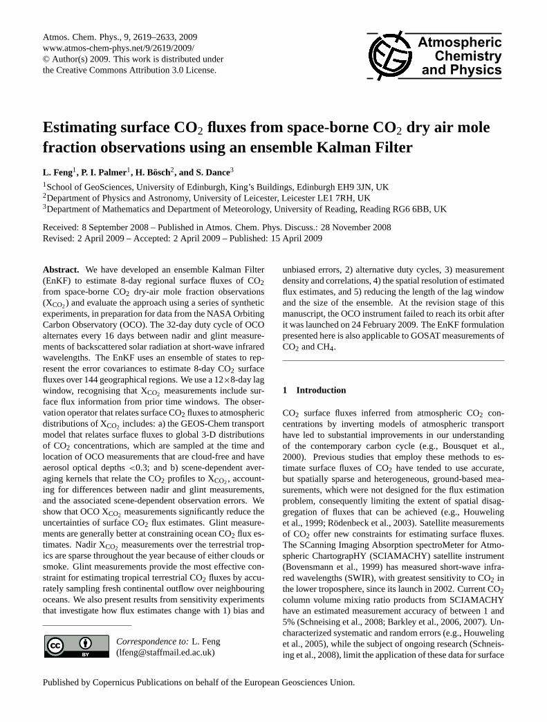
We use averaging kernels as a function of two viewmodes (nadir and glint), five surface types (snow, ocean, soil,conifer, and desert), ten solar zenith angles (SZA) (from 10◦

to 85◦ for nadir measurements, and from 10◦ to 72◦ for glintmeasurements), and seven AODs from 0 to 0.3 (Bosch et al.,2009).

Figure1a and b shows averaging kernels for five differentsurface types at a SZA of 10◦ under a clear-sky with an AODof 0.1. In general, OCO averaging kernels peak in the midand lower troposphere. The instrument sensitivity to changesin CO2 near the surface is particularly important for flux esti-mation. Using nadir view geometry, the oceans are relativelydark at the SWIR wavelengths measured by OCO, and the re-sulting averaging kernels below 400 hPa are lower than overother surface types. In contrast, glint view measurementsover the oceans take advantage of specular reflection, result-ing in a large signal to noise and an averaging kernel close tounity below 400 hPa.

The uncertainty associated with the simulated XCO2 alsodepends on the scene characterization. Figure1c and d showsobservation errors over 5 different surface types as a func-tion of SZA. The error over land is usually<0.5 ppmv for asingle nadir measurement at SZAs<40◦, but increases withSZA, eventually reaching 1.2 ppmv at a SZA of 85◦. Ob-servation errors for nadir measurements over ocean are typ-ically >3.0 ppmv for all SZAs. In contrast, the error for asingle glint measurement over ocean is typically<0.4 ppmv,smaller than nadir errors over land. These errors for mea-surements over lands are smaller than the assumed modeltransport and representation errors (2.5 ppmv), which, as we

Fig. 1. Orbiting Carbon Observatory (OCO) instrument averag-ing kernels (dimensionless) associated with(a) nadir and(b) glintSWIR XCO2 measurements as a function of pressure (hPa) for dif-ferent land types, at a solar zenith angle (SZA) of 10◦ and an aerosoloptical depth (AOD) of 0.1. Observation errors (ppmv) associatedwith (c) nadir and(d) glint XCO2 measurements as function of SZAfor different land types and an AOD of 0.1.

show later, has important implications for flux estimation us-ing these data.

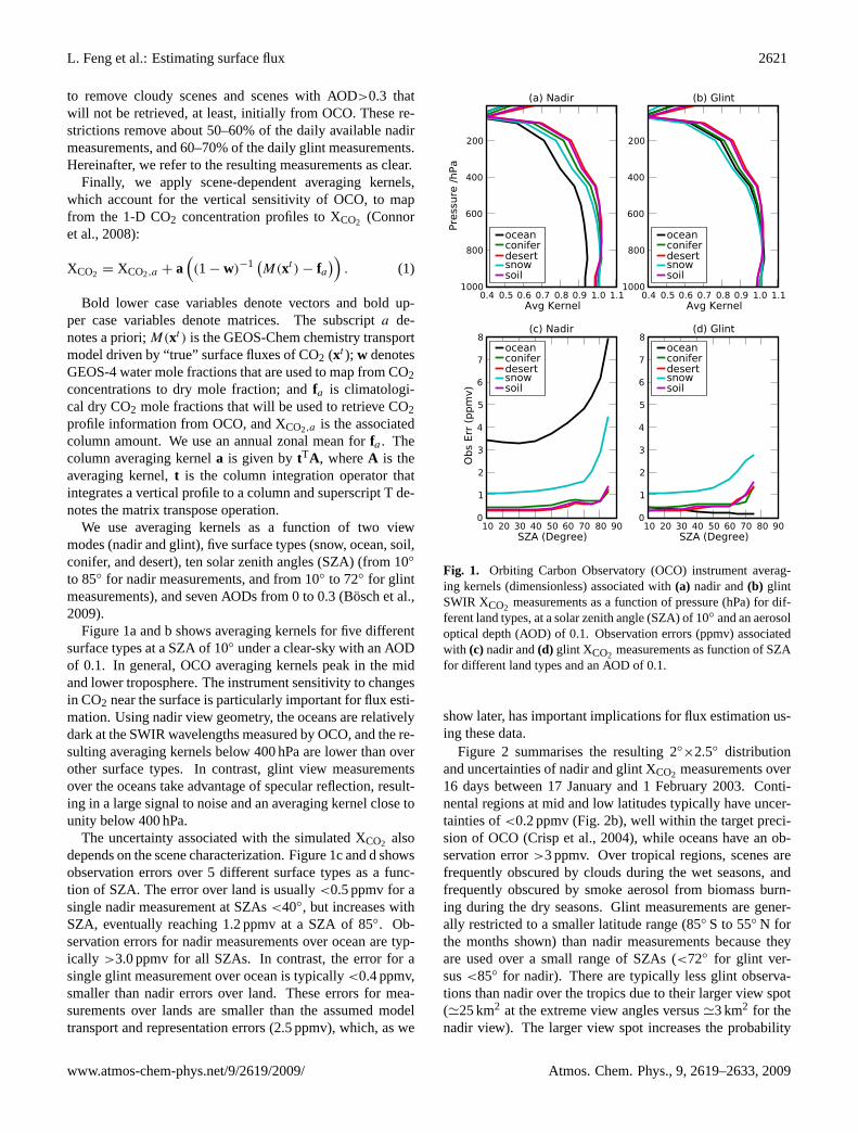
Figure 2 summarises the resulting 2◦×2.5◦ distribution

and uncertainties of nadir and glint XCO2 measurements over16 days between 17 January and 1 February 2003. Conti-nental regions at mid and low latitudes typically have uncer-tainties of<0.2 ppmv (Fig.2b), well within the target preci-sion of OCO (Crisp et al., 2004), while oceans have an ob-servation error>3 ppmv. Over tropical regions, scenes arefrequently obscured by clouds during the wet seasons, andfrequently obscured by smoke aerosol from biomass burn-ing during the dry seasons. Glint measurements are gener-ally restricted to a smaller latitude range (85◦ S to 55◦ N forthe months shown) than nadir measurements because theyare used over a small range of SZAs (<72◦ for glint ver-sus<85◦ for nadir). There are typically less glint observa-tions than nadir over the tropics due to their larger view spot('25 km2 at the extreme view angles versus'3 km2 for thenadir view). The larger view spot increases the probability

www.atmos-chem-phys.net/9/2619/2009/ Atmos. Chem. Phys., 9, 2619–2633, 2009


Fig. 2. Number of clear observations (aerosol optical depth<0.3 and cloud-free) for(a) nadir and(b) glint XCO2 measurements averagedover 16 days from 17 January to 1 February 2003, on a horizontal grid of 2◦

×2.5◦. Associated aggregated errors (ppmv) for the(c) nadirand(d) glint XCO2 measurements.

of cloud obscuration. A similar method is used to define“model” XCO2 distributions for the observation system sim-ulation experiment (OSSE) in Sect.4.

3 The Ensemble Kalman Filter

3.1 Basic formulation

We have developed an ensemble data assimilation systembased on the Ensemble Transform Kalman Filter (ETKF)technique (Bishop et al., 2001) to simultaneously assimilateconsecutive XCO2 observations. At each assimilation cycle,we assimilate 8-day OCO observationsyobs to improve theprior estimation of regional surface CO2 fluxes via:

xa= xf

+ K [yobs− H(xf )] (2)

K = Pf HT[HPf HT

+ R]−1, (3)

wherexf is the a priori state vector;xa is the a posteriori;H is the observation operator that describes the relationshipbetween the state vector and the observations (Sect.2); andK is the Kalman gain matrix that determines the adjustmentto the a priori based on the difference between model and

observations and their uncertainties.R is the observation er-ror covariance matrix, andPf is the a priori error covari-ance matrix.H, the Jacobian of the observation operatorH

(Sect.2), mapsPf into observation space. As mentionedabove in Sect.2, the observation operatorH includes theGEOS-Chem model to describe the atmospheric transport ofCO2, which uses prescribed meteorological analysis; conse-quently, there is no model feedback between CO2 and atmo-spheric dynamics and the transport of CO2 can be consideredas a linear process.

The observation error covarianceR includes measurement(instrument + retrieval) error, model (transport) error and rep-resentation error (Peylin et al., 2002). Quantifying modelerror is non-trivial, and for simplicity we have assumed uni-form model and representation errors: 2.5 ppmv over landregions and 1.5 ppmv over oceans (Rodenbeck et al., 2003),both of which are uncorrelated with the measurement errors.Also, we assume thatR is either diagonal (i.e., no observa-tion correlation, Sect.4.1), or has a simple block structurefor correlations between successive observations (Sect.4.4).

Below we show that our model XCO2 fields are able to in-dependently estimate 8-day mean surface fluxes at a spatialresolution of 1000×1000 km2; estimating at much finer spa-tial resolution introduces strong negative error correlations



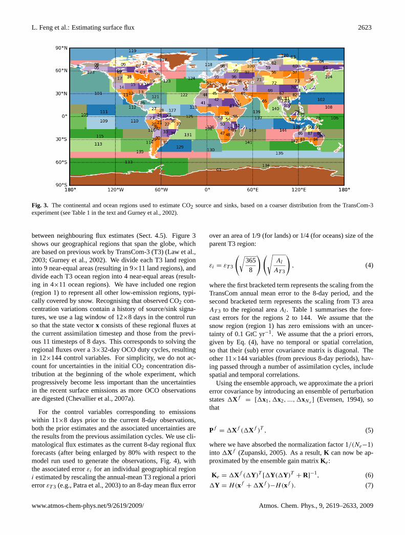
Fig. 3. The continental and ocean regions used to estimate CO2 source and sinks, based on a coarser distribution from the TransCom-3experiment (see Table 1 in the text and Gurney et al., 2002).

between neighbouring flux estimates (Sect.4.5). Figure3shows our geographical regions that span the globe, whichare based on previous work by TransCom-3 (T3) (Law et al.,2003; Gurney et al., 2002). We divide each T3 land regioninto 9 near-equal areas (resulting in 9×11 land regions), anddivide each T3 ocean region into 4 near-equal areas (result-ing in 4×11 ocean regions). We have included one region(region 1) to represent all other low-emission regions, typi-cally covered by snow. Recognising that observed CO2 con-centration variations contain a history of source/sink signa-tures, we use a lag window of 12×8 days in the control runso that the state vectorx consists of these regional fluxes atthe current assimilation timestep and those from the previ-ous 11 timesteps of 8 days. This corresponds to solving theregional fluxes over a 3×32-day OCO duty cycles, resultingin 12×144 control variables. For simplicity, we do not ac-count for uncertainties in the initial CO2 concentration dis-tribution at the beginning of the whole experiment, whichprogressively become less important than the uncertaintiesin the recent surface emissions as more OCO observationsare digested (Chevallier et al., 2007a).

For the control variables corresponding to emissionswithin 11×8 days prior to the current 8-day observations,both the prior estimates and the associated uncertainties arethe results from the previous assimilation cycles. We use cli-matological flux estimates as the current 8-day regional fluxforecasts (after being enlarged by 80% with respect to themodel run used to generate the observations, Fig.4), withthe associated errorεi for an individual geographical regioni estimated by rescaling the annual-mean T3 regional a priorierrorεT 3 (e.g.,Patra et al., 2003) to an 8-day mean flux error

over an area of 1/9 (for lands) or 1/4 (for oceans) size of theparent T3 region:

εi = εT 3

(√365

8

)(√Al

AT 3

), (4)

where the first bracketed term represents the scaling from theTransCom annual mean error to the 8-day period, and thesecond bracketed term represents the scaling from T3 areaAT 3 to the regional areaAl . Table1 summarises the fore-cast errors for the regions 2 to 144. We assume that thesnow region (region 1) has zero emissions with an uncer-tainty of 0.1 GtC yr−1. We assume that the a priori errors,given by Eq. (4), have no temporal or spatial correlation,so that their (sub) error covariance matrix is diagonal. Theother 11×144 variables (from previous 8-day periods), hav-ing passed through a number of assimilation cycles, includespatial and temporal correlations.

Using the ensemble approach, we approximate the a priorierror covariance by introducing an ensemble of perturbationstates1Xf

= [1x1, 1x2, ...,1xNe ] (Evensen, 1994), sothat

Pf= 1Xf (1Xf )T , (5)

where we have absorbed the normalization factor 1/(Ne−1)

into 1Xf (Zupanski, 2005). As a result,K can now be ap-proximated by the ensemble gain matrixK e:

K e = 1Xf (1Y)T [1Y(1Y)T + R]−1, (6)

1Y = H(xf+ 1Xf )−H(xf ). (7)



Table 1. Uncertainty (GtC yr−1) associated with originalTransCom-3 (T3) continental and ocean regions that have been sub-divided for our EnKF inversion. We assume the uncertainty of re-gion 1 (the snow region) to be 0.1 GtC yr−1.

T3 Region Err EnKF Region Err

North American Boreal 0.73 Reg (002–010) 1.64North American Temperate 1.50 Reg (011–019) 3.38

South American Tropical 1.41 Reg (020–028) 3.18South American Temperate 1.23 Reg (029–037) 2.76

North Africa 1.33 Reg (038–046) 3.00South Africa 1.41 Reg (047–055) 3.18

Eurasia Boreal 1.51 Reg (056–064) 3.41Eurasia Temperate 1.73 Reg (065–073) 3.89

Tropical Asia 0.87 Reg(074–082) 1.95Australia 0.59 Reg (083–091) 1.34

Europe 1.42 Reg (092–100) 3.20North Pacific Temperate 0.27 Reg (101–104) 0.61

West Pacific Tropics 0.39 Reg (105–108) 0.88East Pacific Tropics 0.37 Reg (109–112) 0.83

South Pacific Temperate 0.63 Reg (113–116) 1.42Northern Ocean 0.35 Reg (117–120) 0.79

Northen Atlantic Temperate 0.27 Reg (121–124) 0.61Atlantic Tropics 0.41 Reg (125–128) 0.92

South Atlantic Temperate 0.55 Reg (129–132) 1.24South Ocean 0.72 Reg (133–136) 1.62

Indian Tropical 0.48 Reg (137–140) 1.08South Indian Temperate 0.41 Reg (141–144) 0.92

Using the EnKF approach we do not need the Jacobian ma-trix H explicitly to calculate the gain matrixK e.

The EnKF is able to provide a direct estimation of the anal-ysis error covariance. We use the revised, unbiased Ensem-ble Transform Kalman Filter (ETKF) algorithm (Wang et al.,2004; Livings et al., 2008) to determine the analysis ensem-ble1Xa and the a posteriori error covariance,Pa :

1Xa= 1Xf T, (8)

and

Pa= 1Xf T(1Xf T)T . (9)

The transform matrixT is given by

T(T)T = I − (1Y)T [1Y(1Y)T + R]−11Y. (10)

We simplify the calculation of T, K e, and[1Y(1Y)T +R], which is large due to the dense OCOobservations, by using singular value decomposition (SVD)of the scaled model observation ensemble1YT R−1/2

(Livings, 2005).

y, ∆Y

8-day model XCO2

and ensemble

ETKF

xt

8-day mean flux

climatology

GEOS-Chem

xf . ∆Xf

Observed XCO2 Model XCO2

H

Observation operator

8-day forecast

(CO2, H2O etc)

Sample along OCO orbits

Screen for cloud/aerosols

Apply scene-dependent A

H

Observation operator

xf , Pf

Forecast & error

xf=1.8 xt

xf, ∆Xf

forecast & ensemble

yobs , R

8-day OCO XCO2

and error

GEOS-Chem

Sample along OCO orbits

Screen for cloud/aerosols

Apply scene-dependent A

8-day forecast

(CO2, H2O etc)

xa. ∆Xa

Fig. 4. Schematic diagram of the OCO XCO2 Observing SystemSimulation Experiment (OSSE). The left column describes the sim-ulation of OCO XCO2 measurements:xt denotes the “true” fluxes;and H is the observation operator for mapping surface fluxes toXCO2 observationsyobs. It includes the GEOS-Chem global 3-Dtransport model that relates surface fluxes to global 3-D CO2 dis-tributions, which are then sampled along OCO orbits. Scenes withcloud or aerosol optical depths>0.3 are removed. The resultingprofiles are mapped to XCO2 using scene-specific averaging kernels,with associated scene-specific errorR. The right column describesthe simulation of model XCO2 measurements using prior fluxesxf

(80% larger thanxt ) and the associated error covariancePf , whichis approximated by the perturbation state vector ensemble1Xf .Mappingxf and1Xf to the observation space by observation op-eratorH results in the model observationy, and the associated vari-ations1Y. The middle column shows that the Ensemble TransformKalman Filter (ETKF) algorithm generates the optimal estimatexa ,and the a posteriori error covariancePa by comparing the modelforecasts with observations.



3.2 A priori error and its representation

We construct an ensemble of perturbation states to reflect thea priori error covariance matrix, using eigenvalue decompo-sition:

Pf= Vxp1/2

(Vxp1/2

)T

, (11)

whereVx andp are the eigenvector matrix and the eigenvaluediagonal matrix of the error covariance, respectively.

At the limit of using the full-rank matrix, as we do here,the ensemble of perturbation states is defined as:

1Xf= Vxp1/2, (12)

where the matrix1Xf has a size ofNx×Ne, withNx=12×144, and the ensemble sizeNe being equal toNx .When a full-rank representation is used, the Kalman gain ma-trix and the a posteriori error covariance determined fromEq. (6) and Eq. (9) are fully consistent with the ordinaryKalman filter approach (Zupanski, 2005). The most time-consuming part of our EnKF is the projection of the fluxperturbations to the observation space, using the observa-tion operator that includes running a global transport model(Sect.2).

In our sensitivity study, we do not need to re-run the trans-port model for inversions using different observation config-urations. Instead, we define one diagonal matrix1Xf

0 ofthe same size as1Xf , with each column only specifying anemission occurring in one of the twelve 8-day periods overone of the 144 regions. We then calculate the variations inthe observed XCO2 caused by these emissions through theobservation operatorH

1Y0 = H(1Xf

0 ) = H(xf+ 1Xf

0 )−H(xf ). (13)

We can calculate1Y for any given a priori ensemble1Xf

by:

1Y = H(1Xf ) = 1Y0

([1Xf

0 ]−11Xf

). (14)

In practice, we retain only a subset of the column vectorsgiven by Eq. (12), ignoring those associated with small am-plitudes, sufficient to provide a good approximation of theerror covariances (AppendixB). In such a reduced-rank rep-resentation, Eq. (14) becomes invalid.

4 Results

We evaluate our EnKF approach using an observing systemsimulation experiment (OSSE) framework, which is illus-trated in Fig.4. OSSEs have been used extensively to studythe impacts of new observations on data assimilation sys-tems (see for example,Lahoz et al., 2005), but it is widelyrecognised that they can lead to over-optimistic results (At-las, 1997). In our case, we use the same GEOS-Chem trans-port model to generate and assimilate XCO2 measurements.

Such an OSSE framework is not suitable to study the effectsof systematic model errors on inversions. Instead, we focusour OSSE on quantifying the science capabilities of realisticdistributions of XCO2 measurements from space-borne sen-sors.

Observed XCO2 distributions are described in Sect.2,which we regard as the “truth”. Model XCO2 distributionsare defined similarly but we assume the prior flux estimatesto be 80% higher than the “true” values.

First, we present results from a control experiment for a 7-month period from 1 January to 31 July 2003, during whichthe OCO instrument is assumed to operate at the nominal 32-day duty cycle with alternating 16-day nadir and glint mea-surements. We then assess the sensitivity of the a posterioriflux estimates to 1) systematic (bias) and random (unbiased)errors; 2) observation error, density and correlations; 3) al-ternative duty cycles; 4) the spatial resolution of the statevectors; and 5) the length of the lag window and the size ofthe ensemble.

We evaluate the performance of the EnKF by using an er-ror reductionγ

γ = 1 − σ a/σ f , (15)

whereσ f andσ a denote the a priori and a posteriori varianceuncertainties, respectively. For each 8-day mean regionalflux, we calculate itsσ f from the a priori error covarianceat the time when it first enters the lag window, and calculateσ a from the a posteriori error covariance at the time when itleaves the lag window.

The error reductionγ is insensitive to our assumptionsabout the “true” surface fluxes, as well as the values ofthe simulated XCO2 observations. However, approxima-tions in the EnKF approach may lead to underestimation ofthe a posteriori uncertainties (Livings et al., 2008) when areduced-rank representation of the error covariance is used(see Sect.4.6).

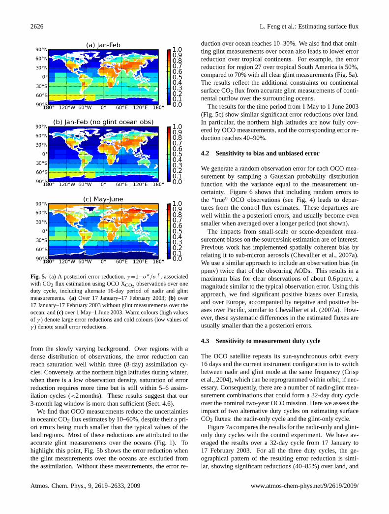
4.1 Control experiment

Figure5 presents the error reduction in the estimates for 8-day mean fluxes over 144 regions. The results have beenaveraged over a 32-day period from 17 January to 17 Febru-ary 2003.

During the northern winter, nadir measurements cover thelatitudes between 90◦ S and 60◦ N, while glint measurementsonly reach 55◦ N. As a result, over most land regions be-tween 30◦ S and 50◦ N, OCO measurements reduce uncer-tainties in the flux estimates by more than 70% (Fig.5a),while errors over the boreal latitudes decrease by 20–65%.The widespread error reduction reflects the coverage and theprecision of nadir and glint measurements. These significantreductions are also related to the large uncertainties in theprior estimates.

We find that most of the error reduction occurs when thecontinental signal is younger than 3 weeks and still distinct



Fig. 5. (a) A posteriori error reduction,γ=1−σ a/σf , associatedwith CO2 flux estimation using OCO XCO2 observations over oneduty cycle, including alternate 16-day period of nadir and glintmeasurements.(a) Over 17 January–17 February 2003;(b) over17 January–17 February 2003 without glint measurements over theocean; and(c) over 1 May–1 June 2003. Warm colours (high valuesof γ ) denote large error reductions and cold colours (low values ofγ ) denote small error reductions.

from the slowly varying background. Over regions with adense distribution of observations, the error reduction canreach saturation well within three (8-day) assimilation cy-cles. Conversely, at the northern high latitudes during winter,when there is a low observation density, saturation of errorreduction requires more time but is still within 5–6 assim-ilation cycles (<2 months). These results suggest that our3-month lag window is more than sufficient (Sect.4.6).

We find that OCO measurements reduce the uncertaintiesin oceanic CO2 flux estimates by 10–60%, despite their a pri-ori errors being much smaller than the typical values of theland regions. Most of these reductions are attributed to theaccurate glint measurements over the oceans (Fig.1). Tohighlight this point, Fig.5b shows the error reduction whenthe glint measurements over the oceans are excluded fromthe assimilation. Without these measurements, the error re-

duction over ocean reaches 10–30%. We also find that omit-ting glint measurements over ocean also leads to lower errorreduction over tropical continents. For example, the errorreduction for region 27 over tropical South America is 50%,compared to 70% with all clear glint measurements (Fig.5a).The results reflect the additional constraints on continentalsurface CO2 flux from accurate glint measurements of conti-nental outflow over the surrounding oceans.

The results for the time period from 1 May to 1 June 2003(Fig. 5c) show similar significant error reductions over land.In particular, the northern high latitudes are now fully cov-ered by OCO measurements, and the corresponding error re-duction reaches 40–90%.

4.2 Sensitivity to bias and unbiased error

We generate a random observation error for each OCO mea-surement by sampling a Gaussian probability distributionfunction with the variance equal to the measurement un-certainty. Figure6 shows that including random errors tothe “true” OCO observations (see Fig.4) leads to depar-tures from the control flux estimates. These departures arewell within the a posteriori errors, and usually become evensmaller when averaged over a longer period (not shown).

The impacts from small-scale or scene-dependent mea-surement biases on the source/sink estimation are of interest.Previous work has implemented spatially coherent bias byrelating it to sub-micron aerosols (Chevallier et al., 2007a).We use a similar approach to include an observation bias (inppmv) twice that of the obscuring AODs. This results in amaximum bias for clear observations of about 0.6 ppmv, amagnitude similar to the typical observation error. Using thisapproach, we find significant positive biases over Eurasia,and over Europe, accompanied by negative and positive bi-ases over Pacific, similar toChevallier et al.(2007a). How-ever, these systematic differences in the estimated fluxes areusually smaller than the a posteriori errors.

4.3 Sensitivity to measurement duty cycle

The OCO satellite repeats its sun-synchronous orbit every16 days and the current instrument configuration is to switchbetween nadir and glint mode at the same frequency (Crispet al., 2004), which can be reprogrammed within orbit, if nec-essary. Consequently, there are a number of nadir-glint mea-surement combinations that could form a 32-day duty cycleover the nominal two-year OCO mission. Here we assess theimpact of two alternative duty cycles on estimating surfaceCO2 fluxes: the nadir-only cycle and the glint-only cycle.

Figure7a compares the results for the nadir-only and glint-only duty cycles with the control experiment. We have av-eraged the results over a 32-day cycle from 17 January to17 February 2003. For all the three duty cycles, the ge-ographical pattern of the resulting error reduction is simi-lar, showing significant reductions (40–85%) over land, and



Fig. 6. The deviations (GtC yr−1) of the estimated CO2 fluxes fromthe “truth” for one duty cycle from 17 January to 17 February 2003.The results have been aggregated from 144 regions (Fig.3) to the22 TransCom-3 regions (see Table 1 in the text and Gurney et al.,2002). Grey line denotes the difference between the a priori and the“truth”, and the black line is the results for the a posteriori in thecontrol run. Red and green lines denote the departures of the a pri-ori from the “truth” in the experiments with systematic or randomobservation errors, respectively. For clarity, the a posteriori errorsin the control run are given as the vertical solid lines. The verticaldashed line demarcates land ocean flux estimates.

moderate reductions (10–65%) over oceans. Because of thewider observation coverage, the nadir-only cycle has betterperformance over northern high latitudes than the other dutycycles. However, glint-only measurements lead to slightlylarger error reductions over the terrestrial tropics, althoughnadir measurements theoretically represent better constraintsfor terrestrial sources and sinks by sampling overhead. Asmentioned previously, we generally find that tropical landmasses are typically characterized by extensive and persis-tent cloud cover during the wet season and by smoke aerosolduring the dry season so the observation density of nadirmeasurements is low. High-precision glint measurements,sampling continental outflow over the oceans, provide im-portant constraints for estimating land flux estimates.

Nadir measurements provide little constraint on oceanCO2 flux estimates, as expected. Glint measurements lead tosignificant reductions of flux errors over the oceans, reach-ing 40–60% over the tropics. The 16-day nadir/glint switchleads to a moderate performance between the glint-only andnadir-only duty cycles.

Fig. 7. Regional a posteriori error reduction,γ=1−σ a/σf , associ-ated with CO2 flux estimation using OCO XCO2 observations overone 32-day duty cycle (17 January–17 February 2003). Results havebeen aggregated from 144 regions (Fig.3) to the 22 TransCom-3 re-gions (see Table 1 in the text and Gurney et al., 2002). The verticalsolid line demarcates land and ocean flux estimates. Significant er-ror reduction (γ>0.5) is marked by the horizontal solid line.(a)Squares denote results from the control run, circles denote resultsfrom using only nadir measurements, and triangles denote resultsfrom using only glint measurements;(b) circles denote results fromusing 80% of available measurements, and triangles denote resultsfrom including spatial correlations in the measurement error covari-anceR with an e-folding length scale of 300 km.

4.4 Sensitivity to observation density and correlation

Figure7b shows that because of the high observation density,reducing the clear observation number by 20% only slightlyincreases the uncertainties of the estimated fluxes over 144regions.

OCO observations are made during daylight, and two con-secutive orbits are separated by about 24◦ in longitude. Toinvestigate the impact of measurement correlations, we as-sume a distance-dependent spatial correlation between obser-vations from the same satellite orbits so that the off-diagonalterm R(m1, m2) for two measurementsm1 and m2 in oneorbit is given as

R(m1, m2)=√

R(m1, m1) R(m2, m2) exp(−l(m1, m2)/ lcor),

(16)



Fig. 8. The sensitivity of error reduction,γ=1−σ a/σf , associatedwith CO2 flux estimation using OCO XCO2 observations over one32-day duty cycle (17 January–17 February 2003), to changes inthe spatial resolution of the state vector. T3 denotes TransCom-3regions that are approximately 9 500 000 km2.

where lcor=300 km is the characteristic spatial correlationlength scale, andl(m1, m2) is the distance between the twomeasurementsm1 andm2. Here we assume that these corre-lations between successive XCO2 arise from both the modeland observation errors. Figure7b shows that imposing aspatial correlation weakens the measurement constraint onflux estimations, as expected. We find the largest impactsfrom including observation correlations are over the oceanswhere there is a greater density of cloud and aerosol-freemeasurements, in agreement withChevallier(2007b). Suc-cessive clear measurements over most land regions are sparseand consequently strong correlations are rare. The associ-ated smaller reduction in error reflects a weaker but possiblymore realistic measurement constraint than used in the con-trol run, but does not suggest that it is a beneficial practice toignore the existing observation correlations in data assimila-tion (Stewart et al., 2008).

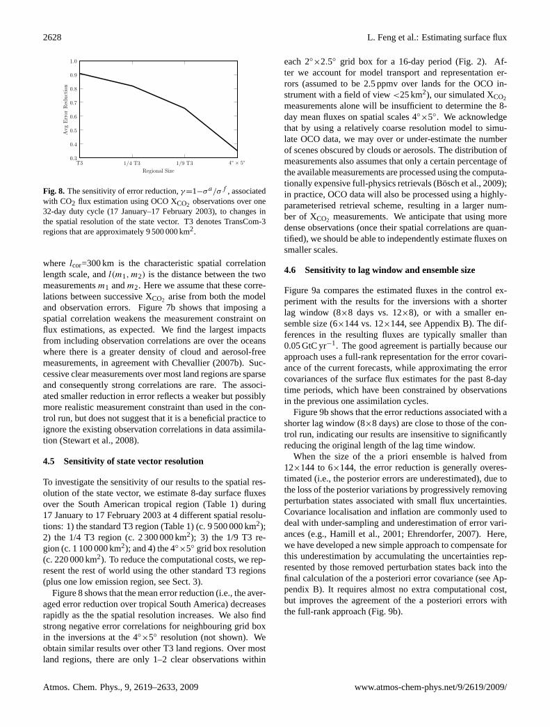
4.5 Sensitivity of state vector resolution

To investigate the sensitivity of our results to the spatial res-olution of the state vector, we estimate 8-day surface fluxesover the South American tropical region (Table1) during17 January to 17 February 2003 at 4 different spatial resolu-tions: 1) the standard T3 region (Table1) (c. 9 500 000 km2);2) the 1/4 T3 region (c. 2 300 000 km2); 3) the 1/9 T3 re-gion (c. 1 100 000 km2); and 4) the 4◦×5◦ grid box resolution(c. 220 000 km2). To reduce the computational costs, we rep-resent the rest of world using the other standard T3 regions(plus one low emission region, see Sect.3).

Figure8 shows that the mean error reduction (i.e., the aver-aged error reduction over tropical South America) decreasesrapidly as the the spatial resolution increases. We also findstrong negative error correlations for neighbouring grid boxin the inversions at the 4◦×5◦ resolution (not shown). Weobtain similar results over other T3 land regions. Over mostland regions, there are only 1–2 clear observations within

each 2◦×2.5◦ grid box for a 16-day period (Fig.2). Af-ter we account for model transport and representation er-rors (assumed to be 2.5 ppmv over lands for the OCO in-strument with a field of view<25 km2), our simulated XCO2

measurements alone will be insufficient to determine the 8-day mean fluxes on spatial scales 4◦

×5◦. We acknowledgethat by using a relatively coarse resolution model to simu-late OCO data, we may over or under-estimate the numberof scenes obscured by clouds or aerosols. The distribution ofmeasurements also assumes that only a certain percentage ofthe available measurements are processed using the computa-tionally expensive full-physics retrievals (Bosch et al., 2009);in practice, OCO data will also be processed using a highly-parameterised retrieval scheme, resulting in a larger num-ber of XCO2 measurements. We anticipate that using moredense observations (once their spatial correlations are quan-tified), we should be able to independently estimate fluxes onsmaller scales.

4.6 Sensitivity to lag window and ensemble size

Figure 9a compares the estimated fluxes in the control ex-periment with the results for the inversions with a shorterlag window (8×8 days vs. 12×8), or with a smaller en-semble size (6×144 vs. 12×144, see AppendixB). The dif-ferences in the resulting fluxes are typically smaller than0.05 GtC yr−1. The good agreement is partially because ourapproach uses a full-rank representation for the error covari-ance of the current forecasts, while approximating the errorcovariances of the surface flux estimates for the past 8-daytime periods, which have been constrained by observationsin the previous one assimilation cycles.

Figure 9b shows that the error reductions associated with ashorter lag window (8×8 days) are close to those of the con-trol run, indicating our results are insensitive to significantlyreducing the original length of the lag time window.

When the size of the a priori ensemble is halved from12×144 to 6×144, the error reduction is generally overes-timated (i.e., the posterior errors are underestimated), due tothe loss of the posterior variations by progressively removingperturbation states associated with small flux uncertainties.Covariance localisation and inflation are commonly used todeal with under-sampling and underestimation of error vari-ances (e.g.,Hamill et al., 2001; Ehrendorfer, 2007). Here,we have developed a new simple approach to compensate forthis underestimation by accumulating the uncertainties rep-resented by those removed perturbation states back into thefinal calculation of the a posteriori error covariance (see Ap-pendix B). It requires almost no extra computational cost,but improves the agreement of the a posteriori errors withthe full-rank approach (Fig.9b).



Fig. 9. (a) CO2 flux errors (GtC yr−1) over one duty cycle from17 January to 17 February 2003. The results have been aggregatedfrom 144 regions (Fig.3) to the 22 TransCom-3 regions (see Ta-ble 1 in the text and Gurney et al., 2002). The squares denote theresults for the control experiment, the circles denote the experimentusing a shorter (8×8 days vs. 12×8 days) lag window, and the tri-angles denote the experiment using half the ensemble size (6×144vs. 12×144). (b) A posteriori error reduction,γ=1−σ a/σf , asso-ciated with regional fluxes shown in (a). Crosses denote the errorreductions when we have compensated for the underestimated pos-terior uncertainties due to the reduced-rank representation of theEnKF.

5 Conclusions

We developed an ensemble Kalman Filter (EnKF) to esti-mate 8-day regional surface fluxes of CO2 from space-borneCO2 dry-air mole fraction observations (XCO2) and evalu-ated the approach using a series of synthetic experiments, inpreparation for data from the NASA Orbiting Carbon Ob-servatory (OCO). The 32-day duty cycle of OCO alternatesbetween nadir and glint (specular reflection) measurementsof backscattered solar radiation at short-wave infrared wave-lengths. Our EnKF represents a complementary approach tothe variational techniques that have already been developedfor interpreting the space-borne XCO2 data (e.g.,Chevallieret al., 2007a). The main advantages of the EnKF is thatit does not require an adjoint model for the forecast andobservation operators, and provides a direct estimation ofthe uncertainty of a posteriori fluxes. We use the ensemble

transform Kalman Filter algorithm to determine the ensem-ble analysis and its error covariance.

For this work, we estimate 8-day CO2 surface fluxes over144 geographical regions (corresponding to 1 100 000 km2

over land), based on the TransCom-3 experiments (Gurneyet al., 2002). We use a 12×8-day lag window, taking intoaccount that XCO2 measurements include surface flux infor-mation from prior time windows. The observation opera-tor relates surface CO2 fluxes to the global distributions ofthe “observed” XCO2. First, we use the GEOS-Chem trans-port model to relate surface fluxes to global 3-D distributionsof CO2 concentrations. Second, these distributions are sam-pled at the time and location of OCO measurements to re-move cloudy scenes and scenes with aerosol optical depth(AOD)>0.3. Finally, we use scene-dependent averaging ker-nels to relate the CO2 profiles to XCO2. We use the scene-dependent measurement errors that correspond to the aver-aging kernels. These scene-dependent calculations provideus with the most realistic simulation of XCO2 distributions todate, with which to understand potential of OCO to estimatesurface CO2 fluxes. We use the same observation operator tomodel atmospheric distributions of XCO2, but with an 80%bias in the prior surface emissions.

We show that OCO XCO2 measurements significantly re-duce the uncertainties of surface CO2 flux estimates, con-sistent with previous studies (Baker et al., 2006; Cheval-lier et al., 2007a; Chevallier, 2007b). We find that nadirmeasurements are better at estimating land-based fluxes andglint measurements are generally better at constraining oceanfluxes. Nadir XCO2 measurements over the terrestrial trop-ics are typically sparse throughout the year because of eitherwidespread and persistent cloud cover during the wet seasonor smoke aerosol associated with extensive biomass burningduring the dry season. We find that glint measurements overthe oceans provide the most effective constraint for estimat-ing terrestrial CO2 fluxes by accurately sampling fresh con-tinental outflow over neighbouring oceans.

We also presented the results from sensitivity experimentsto investigate how flux estimates change with 1) bias and un-biased errors, 2) alternative duty cycles, 3) measurement den-sity and correlations, 4) the spatial resolution of estimatedflux estimates, and 5) reducing the length of the lag windowand the size of the ensemble. We find that biases in the obser-vations, which we introduce by scaling the error using AOD(by a factor of two), cause large perturbations to some of theposterior fluxes but they are still within the posterior uncer-tainties of the control experiment. In real observations, theremay be larger systematic errors than we discuss here, andtheir effects will require further investigation. We find thateither the current 32-day duty cycle (alternating 16-day cy-cle between glint and nadir measurements) or one that usesonly glint view measurements will address the primary sci-ence objectives of the OCO mission, a reflection of the im-portance of glint measurements in constraining tropical ter-restrial fluxes. A modest 20% reduction in the number of



available clear observations does not affect a posteriori re-gional flux estimates, reflecting the high measurement den-sity. Introducing a spatial correlation between successivemeasurements effectively reduces the number of independentobservations. We find that spatial correlations mainly affectglint measurements over the oceans where there is a greaternumber of neighbouring scenes that are cloud-free and haveAODs<0.3. We find that reducing the size of the geographi-cal regions over which to estimate surface fluxes much below1 million km2 introduces large correlations between neigh-bouring regional estimates. In the control experiment, wesimultaneously estimate surface fluxes at the time of the as-similation and at times up to 3 months prior. We find thatsurface flux estimates for a particular 8-day period typicallyconverge after ingesting 4–6 weeks of data. To improve thespeed of the EnKF we halved the number of ensemble statesused to determine the a priori error covariance and showedthat the flux estimates were close to the control experimentbut using a reduced number of ensemble states, we generallyunderestimated the associated error. Constructing efficientreduced-rank representations of the EnKF, and the methodsto compensate for associated underestimation of the poste-rior uncertainties, necessary to reduce computational costsrelated to estimating fluxes on finer spatial resolutions, is thesubject of ongoing work.

In light of the failed OCO launch (Palmer and Rayner,2009), we will focus our developed EnKF on GOSAT mea-surements of CO2 and CH4. This will require informationabout the GOSAT orbit, sampling strategy, and retrieval er-ror diagnostics that will soon become available. We antici-pate that application of the EnKF to GOSAT data will differonly slightly to the application to OCO data shown in thispaper, e.g., length of the assimilation window, which will bethe subject of further work.

Appendix A

Description of the GEOS-Chem Modelof Atmospheric CO2

We use the GEOS-Chem global 3-D chemistry transportmodel (v7-03-06) to calculate XCO2 concentrations from pre-scribed surface CO2 fluxes described below. We used themodel with a horizontal resolution of 2◦

×2.5◦, and 30 verti-cal levels (derived from the native 48 levels) ranging from thesurface to the mesosphere, 20 of which are below 12 km. Themodel is driven by GEOS-4 assimilated meteorology datafrom the Global Modeling and Assimilation Office GlobalCirculation Model based at NASA Goddard. The 3-D me-teorological data is updated every six hours, and the mixingdepths and surface fields are updated every three hours. TheCO2 simulation is based onSuntharalingam et al.(2005) andPalmer et al.(2006, 2008).

We use gridded fossil fuel emission distributions, repre-sentative of 1995 (Suntharalingam et al., 2005), which wehave scaled to 2003 values using regional budget estimatesfor the top 20 emitting countries in 2003 from the CarbonDioxide Information Analysis Center (Marland et al., 2007).Biofuel emission estimates are taken fromYevich and Logan(2003) and represent climatological values. Monthly meanbiomass burning emission estimates are taken from the sec-ond version of the Global Fire Emission Database (GFEDv2)for 2003 (van der Werf et al., 2006), which are derived fromground-based and satellite observations. Daily mean landbiosphere fluxes are taken from the CASA model for 2001(Randerson et al., 1997), in the absence of correspondingfluxes for 2003. We do not explicitly account for the con-tribution of fuel combustion CO2 from the oxidation of re-duced carbon species (Suntharalingam et al., 2005) as theymake only a small contribution to the CO2 column. Monthlymean air-sea fluxes of CO2 are taken from (Takahashi et al.,1999).

CO2 concentrations for January 2002 were initialized froma previously evaluated model run (Palmer et al., 2006), whichwe integrate forward to January 2003. We include an ad-ditional initialization to correction for the model bias intro-duced by not accounting for the net uptake of CO2 fromthe terrestrial biosphere. We make this downward correctby comparing the difference between GLOBALVIEW CO2data (GLOBALVIEW-CO2) and model concentrations overthe Pacific during January 2003. Differences range from 1 to4 ppmv with a median of 3.5 ppmv, and we subtract this valueglobally, followingSuntharalingam et al.(2005). From Jan-uary 2003 the total CO2 tracer becomes the “background”CO2 concentration and is only subject to atmospheric trans-port. At that time, we also introduce additional model trac-ers, initialized with a uniform value (for numerical reasonsand which is subtracted in subsequent analyses), that ac-count for the monthly production and loss of CO2 originat-ing from specific geographical regions and surface processes(“tagged” tracers). The linear sum of these monthly taggedtracers (and the “background”) is equivalent to the total CO2.

Appendix B

Description of the reduced representationof a priori error covariance

To reduce the computational costs of our EnKF approach, weuse a reduced-rank representation to approximate the a priorierror covariances, so that fewer ensemble states need to beprojected to the observation space using the observation op-eratorH that includes a global 3-D transport model of CO2.

As mentioned in Sect.3, during thej -th cycle of assimi-lating XCO2 observations from dayd to d+8, our state vectorconsists of 1) the current forecast of the regional surface CO2



fluxes from dayd to d+8, and 2) the 8-day mean regionalflux estimates from time periods prior to dayd.

We assume no error correlation between the current fore-cast and the previous analysisxa

j−1, and hence the prior errorcovariance at the assimilation cyclej consists of two blocks:1) the error covariance of the current forecast; and 2) the er-ror covariance ofxa

j−1.The error covariance of the current forecast is a diagonal

matrix of sizeNr×Nr (Sect.3), whereNr is the numberof the global regions (Nr=144 in the control run). In thereduced-rank approach discussed here, we still useNr newperturbation states1Xp1

j to represent this diagonal error co-variance matrix.

But we only choose a subset of the a posteriori ensembleof the previous cycle to approximate the error covariance ofthe estimates over the past time periods in the steps describedbelow.

For clarity, we start by calculating the a posteriori ensem-ble at the end of the previous assimilation cyclej−1 viaEq. (8), where the subscript denotes the assimilation cyclenumber:

1Xaj−1 = 1Xf

j−1Tj−1. (B1)

Matrix 1Xaj−1 is the same size of matrix1Xf

j−1, whichconsists ofNe columns, each withNx elements representingperturbations in the regional 8-day mean surface CO2 fluxesprior to the current dayd.

We then use SVD to decompose1Xaj−1:

1Xaj−1 = Ua

j−16aj−1(V

aj−1)

T , (B2)

whereUaj−1, andVa

j−1 are two orthogonal matrices of sizeNx×Nx andNe×Ne, respectively, and6a

j−1 is a diagonalmatrix of sizeNx×Ne, with its non-zero diagonal elementspresenting the singular values of matrix1Xa

j−1 in descend-ing order of magnitude.

By applyingVaj−1 to Eq. (B2), we obtain

1Xcj = 1Xa

j−1Vj−1 = Uaj−16

aj−1. (B3)

Matrix 1Xcj has the same size as1Xa

j−1, and satisfies

Paj−1=1Xa

j−1(1Xaj−1)

T=1Xc

j−1(1Xcj−1)

T (B4)

We divide the ensemble1Xcj=[1xc

1, 1xc2, ...,1xc

Ne] into

two subsets: 1) the major subset1Xp2j that consists of its

first Nb columns; and 2) the minor subset1Xsj for its last

Ne−Nb columns. The two subsets together satisfy

Paj−1 = 1Xp2

j (1Xp2j )T + 1Xs

j (1Xsj )

T . (B5)

The major subset1Xbj contains the columns with the largest

amplitudes, and in principle, a suitable choice ofNb ensuresthat Pp2

j = 1Xp2j (1Xp2

j )T provides a good approximationof the error covariancePa

j−1, while the uncertainties repre-

sented byPsj=1Xs

j (1Xsj )

T are small enough to be ignored.

In this study, we chooseNb to be equal toNe−Nr (in thespin-up period where the lag window is shorter than 12×8days,Nb is chosen to increase with the size of the state vectortill it reaches the pre-defined ensemble sizeNe). Combiningthe resulting ensemble1Xp2

j and1Xp1j provides a reduced-

rank representation of the prior uncertainties of the currentassimilation cyclej .

During the previous assimilation cycle, the GEOS-Chemmodel run, forced by its prior surface flux estimates, alsogenerates an estimate of the 3-D CO2 concentrationscf

j−1 atthe beginning of dayd. Similar simulations for the a prioriensemble1Xf

j−1 provide an ensemble of 3-D CO2 concen-

trations1Cf

j−1 for the variations caused by the perturbationsin the surface CO2 fluxes. We calculate the “analysis” ofthe 3-D CO2 concentrations fromcf

j−1 and1Cf

j−1 using anequation similar to Eq. (2), and generate the variations corre-sponding to1Xp2

j by selecting the firstNb fields from matrix

1Ccj = 1Cf

j−1Tj−1Vj−1.In the current assimilation cycle over dayd to dayd+8,

we use the GEOS-Chem transport model to propagate theseresulting CO2 fields to the current observation space to ac-count the contributions from the surface CO2 fluxes prior todayd.

The reduced-rank representation tends to underestimatethe a posteriori error covariance. To compensate for this un-derestimation, we accumulate the previously ignored smalluncertaintiesPs

j into the calculation of the final a posteri-ori error covariance at the time the regional fluxes estimatesover dayd to dayd+8 leave the lag window of 12×8 days,after having been constrained by observations in 12 consec-utive assimilation cycles. This compensation is consistentwith the assumption that these previously ignored uncertain-ties are too small to be significantly reduced by ingesting ob-servations.

Acknowledgements.This study is funded by the UK NaturalEnvironment Research Council under NE/F000014/1. Work at theJet Propulsion Laboratory (JPL), California Institute of Technologywas carried out under a contract with the National Aeronautics andSpace Administration.

Edited by: W. Lahoz

References

Atlas, R: Atmospheric observations and experiments to assess theirusefulness in data assimilation, J. Meteorol. Soc. Japan, 75 (1B),111–130,1997.

Baker, D. F., Doney, S. C., and Schimel, D. S.: Variational dataassimilation for atmospheric CO2, Tellus Ser. B, 58, 359–365,2006.

Barkley, M. P., Monks, P. S., Frieß, U., Mittermeier, R. L., Fast,H., Korner, S., and Heimann, M.: Comparisons between SCIA-MACHY atmospheric CO2 retrieved using (FSI) WFM-DOAS toground based FTIR data and the TM3 chemistry transport model,



Atmos. Chem. Phys., 6, 4483–4498, 2006,http://www.atmos-chem-phys.net/6/4483/2006/.

Barkley, M. P., Monks, P. S., Hewitt, A. J., Machida, T., Desai, A.,Vinnichenko, N., Nakazawa, T., Yu Arshinov, M., Fedoseev, N.,and Watai, T.: Assessing the near surface sensitivity of SCIA-MACHY atmospheric CO2 retrieved using (FSI) WFM-DOAS,Atmos. Chem. Phys., 7, 3597–3619, 2007,http://www.atmos-chem-phys.net/7/3597/2007/.

Bishop, C. H., Etherton, B. J., and Majumdar, S. J.: Adaptive Sam-pling with the Ensemble Transform Kalman Filter. Part I: Theo-retical Aspects, Mon. Weather Rev., 129, 420–436, 2001.

Bosch, H., Baker, D., Connor, B., O’Brien, D., Crisp, D., andMiller, C.: Global Characterization of XCO2 Retrievals fromOCO Observations, in preparation, 2009.

Bousquet, P., Peylin, P., Ciais, P., Quere, C. L., Friedlingstein, P.,and Tans, P. P.: Regional changes in carbon dioxide fluxes ofland and oceans since 1980, Science, 290, 1342–1346, 2000.

Bovensmann, H., Burrows, J., Buchwitz, M., Frerick, J., Noel, S.,Rozanov, V., Chance, K. V., and Goede, A.: SCIAMACHY: Mis-sion objectives and measurement modes, J. Atmos. Sci., 56, 127–150, 1999.

Bruhwiler, L. M. P., Michalak, A. M., Peters, W., Baker, D. F., andTans, P.: An improved Kalman Smoother for atmospheric inver-sions, Atmos. Chem. Phys., 5, 2691–2702, 2005,http://www.atmos-chem-phys.net/5/2691/2005/.

Chevallier, F.: Impact of correlated observation errors on invertedCO2 surface fluxes from OCO measurements, Geophys. Res.Lett., 34, L24804, doi:10.1029/2007GL030463, 2007b.

Chevallier, F., Breon, F.-M., and Rayner, P. J.: Contribution of theOrbiting Carbon Observatory to the estimation of CO2 sourcesand sinks: Theoretical study in a variational data assimila-tion framework, J. Geophys. Res., 112, D09307, doi:10.1029/2006JD007375, 2007a.

Chevallier, F. M. F., Peylin, P., Bousquet, S. S. P., Breon, F.-M.,Chedin, A., and Ciais, P.: Inferring CO2 sources and sinks fromsatellite observations: Method and application to TOVS data, J.Geophys. Res., 110, D24309, doi:10.1029/2005JD006390, 2005.

Connor, B. J., Bosch, H., Toon, G., Sen, B., Miller, C., andCrisp, D.: Orbiting Carbon Observatory: Inverse method andprospective error analysis, J. Geophys. Res., 113, D05305, doi:10.1029/2006JD008336, 2008.

Crisp, D., Atlas, R. M., Breon, F. -M., et al.: The Orbiting CarbonObservatory (OCO) Mission, Adv. Space. Res., 34(4), 700–709,2004.

Ehrendorfer, M.: A review of issues in ensemble-based Kalman fil-tering, Meteorol. Z., 16, 795–818, 2007.

Evensen, G.: Sequential data assimilation with a nonlinear quasi-geostrophic model using Monte Carlo methods to forecast errorstatistics, J. Geophys. Res., 99(C5), 10143–10162, 1994.

Evensen, G.: The Ensemble Kalman Filter: Theoretical formula-tion and practical implementation, Ocean Dynam., 53, 343–367,2003.

GLOBALVIEW-CO2: Cooperative Atmospheric Data Project Car-bon Dioxide, CD-ROM, NOAA GMD, Boulder, Colorado,USA (also available via anonymous FTP toftp.cmdl.noaa.gov,path:/ccg/co2/GLOBALVIEW, 2006.

Gurney, K. R., Law, R. L., Denning, A. S., et al.: Towards robustregional estimates of CO2 sources and sinks using atmospherictransport models, Nature, 415, 626–630, 2002.

Hamill, T. M., Whitaker, J. S., and Snyder, C.: Distance-DependentFiltering of Background Error Covariance Estimates in an En-semble Kalman Filter, Mon. Weather Rev., 129, 2776–2790,2001.

Houtekamer, P. L. and Mitchell, H. L.: Data assimilation using anensemble Kalman filter technique, Mon. Weather Rev., 126, 796–811, 1998.

Houweling, S., Kaminski, T., Dentener, F., Lelieveld, J., andHeimann, M.: Inverse modeling of methane sources and sinksusing the adjoint of a global transport model, J. Geophys. Res.,104, 26137–26160, 1999.

Houweling, S., Hartmann, W., Aben, I., Schrijver, H., Skidmore, J.,Roelofs, G.-J., and Breon, F.-M.: Evidence of systematic errorsin SCIAMACHY-observed CO2 due to aerosols, Atmos. Chem.Phys., 5, 3003–3013, 2005,http://www.atmos-chem-phys.net/5/3003/2005/.

Lahoz, W. A., Brugge, R., Jackson, D. R., Migliorini, S., Swinbank,R., Lary, D., and Lee, A.: An observing system simulation ex-periment to evaluate the scientific merit of wind and ozone mea-surements from the future SWIFT instrument, Q. J. Roy. Meteor.Soc., 131, 503–523, doi:10.1256/qj.03.109, 2005.

Law, R. M., Chen, Y. H., and Gurney, K. R.: TransCom-3 CO2inversion intercomparison: 2. Sensitivity of annual mean resultsto data choices, Tellus, Ser. B, 55, 580–595, 2003.

Livings, D. M.: Aspects of the Ensemble Kalman Filter, M.Sc. the-sis, Department of Mathematics, University of Reading, UK, 34–37, 2005.

Livings, D. M., Dance, S. L., and Nichols, N. K.: Unbiased ensem-ble square root filters, Physica D., 237/8, 1021–1028, 2008.

Lorenc, A. C.: The potential of the ensemble Kalman filter forNWP–A comparison with 4D-Var, Q. J. Roy. Meteor. Soc., 129,3183–3203, 2003.

Maksyutov, S., Kadygrov, N., Nakatsuka, Y., Patra, P. K.,Nakazawa, T., Yokota, T., and Inoue, G.: Projected impact ofthe GOSAT observations on regional CO2 flux estimations as afunction of total retrieval error, Journal of Remote Sensing Soci-ety of Japan, 28, 190–197, 2008.

Marland, G., Boden, T. A., and Andres, R. J.: Global, Regional,And National CO2 Emissions, in Trends: A Compendium ofData on Global Change, Tech. Rep. 2007, 7346, Carbon DioxideInformation Analysis Center Oak Ridge National Laboratory, USDepartment of Energy, Oak Ridge, Tenn., USA, 2007.

Miller, C. E., Crisp, D., DeCola, P. L., et al.: Precision requirementsfor space-based XCO2 data, J. Geophys. Res, D10314, doi:10.1029/2006JD007659, 2007.

Palmer, P. I., Suntharalingam, P., Jones, D. B. A., Jacob, D. J.,Streets, D. G., Fu, Q., Vay, S. A., and Sachse, G. W.: Us-ing CO2:CO correlations to improve inverse analyses of car-bon fluxes, J. Geophys. Res., 111, D12318, doi:10.1029/2005JD006697, 2006.

Palmer, P. I., Barkley, M. P., and Monks, P. S.: Interpreting thevariability of space-borne CO2 column-averaged volume mixingratios over North America using a chemistry transport model,Atmos. Chem. Phys., 8, 5855–5868, 2008,http://www.atmos-chem-phys.net/8/5855/2008/.

Palmer, P. I. and Rayner, P.: Failure to launch, Nature Geosci., 2,247, doi:10.1038/ngeo495, 2009.

Patra, P. K., Maksyutov, S., Sasano, Y., Nakajima, H., Inoue, G.,and Nakazawa, T.: An evaluation of CO2 observations with So-


http://www.atmos-chem-phys.net/6/4483/2006/



ftp.cmdl.noaa.gov




lar Occultation FTS for Inclined-Orbit Satellite sensor for sur-face source inversion, J. Geophys. Res., 108(D24), 4759, doi:10.1029/2003JD003661, 2003.

Peters, W., Miller, J. B., Whitaker, J., Denning, A. S., Hirsch, A.,Krol, M. C., Zupanski, D., Bruhwiler, L., and Tans, P. P.: An en-semble data assimilation system to estimate CO2 surface fluxesfrom atmospheric trace gas observations, J. Geophys. Res., 110,D24304, doi:10.1029/2005JD006157, 2005.

Peylin, P., Baker, D., Sarmiento, J., Ciais, P., and Bousquet, P.: In-fluence of transport uncertainty on annual mean and seasonal in-versions of atmospheric CO2 data, J. Geophys. Res., 107(D19),4385, doi:10.1029/2001JD000857, 2002.

Potter, C. S., Randerson, J. T., Field, C. B., Matson, P. A., Vitousek,P. M., Mooney, H. A., and Klooster, S. A.: Terrestrial ecosys-tem production: A process model based on global satellite andsurface data, Global Biogeochem. Cy., 7(4), 811–842, 1993.

Randerson, J. T., Thompson, M. V., Conway, T. J., Fung, I. Y., andField, C. B.: The contribution of terrestrial sources and sinksto trends in the seasonal cycle of atmospheric carbon dioxide,Global Biogeochem. Cy., 11(4), 535–560, 1997.

Rayner, P. J., Law, R. M., O’Brien, D. M., Butler, T. M., and Dilley,A. C.: Global observations of the carbon budget: 3. Initial assess-ment of the impact of satellite orbit, scan geometry, and cloud onmeasuring CO2 from space, J. Geophys. Res., 107(D21), 4557,doi:10.1029/2001JD000618, 2002.

Rodenbeck, C., Houweling, S., Gloor, M., and Heimann, M.: CO2flux history 1982–2001 inferred from atmospheric data using aglobal inversion of atmospheric transport, Atmos. Chem. Phys.,3, 1919–1964, 2003,http://www.atmos-chem-phys.net/3/1919/2003/.

Schneising, O., Buchwitz, M., Burrows, J. P., Bovensmann, H.,Reuter, M., Notholt, J., Macatangay, R., and Warneke, T.: Threeyears of greenhouse gas column-averaged dry air mole fractionsretrieved from satellite – Part 1: Carbon dioxide, Atmos. Chem.Phys., 8, 3827–3853, 2008,http://www.atmos-chem-phys.net/8/3827/2008/.

Stewart, L. M., Dance, S., and Nichols, N.: Information contentand correlated observation errors, Int. J. Numer. Meth. Fl., 56,1521–1527, 2008.

Suntharalingam, P., Randerson, J. T., Krakauer, N., Logan, J. A.,and Jacob, D. J.: The influence of reduced carbon emissions andoxidation on the distribution of atmospheric CO2: implicationsfor inversion analysis, Global Biogeochem. Cy., 19, GB4003,doi:10.1029/2005GB002466, 2005.

Takahashi, T., Wanninkhof, R. T., Feely, R. A., Weiss, R. F., Chap-man, D. W., Bates, N. R., Olafsson, J., Sabine, C. L., andSutherland, C. S.: Net sea-air CO2 flux over the global oceans,proceedings of the 2nd international symposium CO2 in theoceans: CGER 1037, National Institute for Environmental Stud-ies, Tsukuba, Japan, 915 pp., 1999.

Takahashi, T., Sutherland, S. C., Sweeney, C., et al.: Global sea-air CO2 flux based on climatological surface ocean pCO2, andseasonal biological and temperature effects, Deep Sea Res., PartII, 49, 1601–1622, 2002.

Tiwari, Y. K., Gloor, M., Engelen, R. J., Chevallier, F., Rodenbeck,C., Korner, S., Peylin, P., Braswell, B. H., and Heimann, M.:Comparing CO2 retrieved from Atmospheric Infrared Sounderwith model predictions: Implications for constraining surfacefluxes and lower-to-upper troposphere transport, J. Geophys.Res., 111, D17106, doi:10.1029/2005JD006681, 2006.

van der Werf, G. R., Randerson, J. T., Giglio, L., Collatz, G. J.,Kasibhatla, P. S., and Arellano Jr., A. F.: Interannual variabilityin global biomass burning emissions from 1997 to 2004, Atmos.Chem. Phys., 6, 3423–3441, 2006,http://www.atmos-chem-phys.net/6/3423/2006/.

Wang, X., Bishop, C. H., and Julier, S. J.: Which is better, an en-semble of positive-negative pairs or a centered spherical simplexensemble, Mon. Weather Rev., 132, 1590–1605, 2004.

Yevich, R. and Logan, J. A.: An assessment of biofuel use and burn-ing of agricultural waste in the developing world, Global Bio-geochem. Cy., 17, 1095, doi:10.1029/2002GB001952, 2003.

Zupanski, M.: Maximum likelihood Ensemble Filter: TheoreticalAspects, Mon. Weather Rev., 133, 1710–1726, 2005.





Documents

Estimating surface CO ﬂuxes from space-borne CO dry air ... · PDF filelar Occultation FTS for Inclined-Orbit Satellite sensor for sur-face source inversion, J. Geophys. Res., 108(D24),