FLORIDA STATE UNIVERSITY

COLLEGE OF ARTS AND SCIENCES

ESTIMATING THE EFFECTS OF CLIMATE CHANGE

ON TROPICAL CYCLONE ACTIVITY

By

CHANA SEITZ

A Thesis submitted to theDepartment of Earth, Ocean, and Atmospheric Sciences

in partial fulfillment of therequirements for the degree of

Master of Science

Degree Awarded:Spring Semester, 2014

Copyright c© 2014 Chana Seitz. All Rights Reserved.

Chana Seitz defended this thesis on March 18, 2014.The members of the supervisory committee were:

Vasu Misra

Professor Co-Directing Thesis

Timothy LaRow

Professor Co-Directing Thesis

Robert Hart

Committee Member

Philip Sura

Committee Member

The Graduate School has verified and approved the above-named committee members, and certifiesthat the thesis has been approved in accordance with university requirements.

ii

I dedicate this thesis to my mother, Kandra Garmier.

iii

ACKNOWLEDGMENTS

I would like to thank Dr. LaRow for helping me learn the process of scientific research. I would like

to thank my committee members (Dr. Hart, Dr. LaRow, Dr. Misra, and Dr. Sura) for devoting

time to being on my committee and for helping me improve my work. I would like to thank all of

my co-workers and friends at COAPS and on campus for providing a great working environment

and for always being open to scientific discussion. I would like to thank all of my friends outside

of work and school for supporting my interest in Meteorology and staying in touch despite the

distance I moved to continue my education. Finally, I would like to thank my family members for

encouraging me to attend graduate school and for supporting me throughout every part of my life

has that led me to this point.

iv

TABLE OF CONTENTS

List of Tables . . . . . . . . . . . . . . . . . . . . . . . . . . . . . . . . . . . . . . . . . . . . . vii

List of Figures . . . . . . . . . . . . . . . . . . . . . . . . . . . . . . . . . . . . . . . . . . . . viii

List of Abbreviations . . . . . . . . . . . . . . . . . . . . . . . . . . . . . . . . . . . . . . . . . x

Abstract . . . . . . . . . . . . . . . . . . . . . . . . . . . . . . . . . . . . . . . . . . . . . . . . xi

1 Introduction 11.1 The Predictability of Tropical Cyclone Climatology . . . . . . . . . . . . . . . . . . . 1

1.1.1 Theory . . . . . . . . . . . . . . . . . . . . . . . . . . . . . . . . . . . . . . . 11.1.2 Modeling Tropical Cyclone Climatology . . . . . . . . . . . . . . . . . . . . . 2

1.2 Environmental Influences on Tropical Cyclone Activity . . . . . . . . . . . . . . . . . 31.3 Motivation . . . . . . . . . . . . . . . . . . . . . . . . . . . . . . . . . . . . . . . . . 41.4 Results of Similar Research . . . . . . . . . . . . . . . . . . . . . . . . . . . . . . . . 41.5 Research Goals . . . . . . . . . . . . . . . . . . . . . . . . . . . . . . . . . . . . . . . 5

2 Method 72.1 Representative Concentration Pathways (RCPs) . . . . . . . . . . . . . . . . . . . . . 72.2 SST Discussion . . . . . . . . . . . . . . . . . . . . . . . . . . . . . . . . . . . . . . . 82.3 Experiment Design . . . . . . . . . . . . . . . . . . . . . . . . . . . . . . . . . . . . . 162.4 Plan for Analysis . . . . . . . . . . . . . . . . . . . . . . . . . . . . . . . . . . . . . . 17

3 Results and Discussion 193.1 NTC Statistics by Domain . . . . . . . . . . . . . . . . . . . . . . . . . . . . . . . . . 19

3.1.1 NTC Counts . . . . . . . . . . . . . . . . . . . . . . . . . . . . . . . . . . . . 193.1.2 NTC Duration . . . . . . . . . . . . . . . . . . . . . . . . . . . . . . . . . . . 233.1.3 NTC Annual Maximum 10-Meter Wind Speed . . . . . . . . . . . . . . . . . 243.1.4 NTC Daily Precipitation . . . . . . . . . . . . . . . . . . . . . . . . . . . . . 27

3.2 Genesis and Track Density . . . . . . . . . . . . . . . . . . . . . . . . . . . . . . . . . 303.2.1 NTC Genesis Density . . . . . . . . . . . . . . . . . . . . . . . . . . . . . . . 303.2.2 NTC Track Density . . . . . . . . . . . . . . . . . . . . . . . . . . . . . . . . 32

3.3 NTC Annual Cycles . . . . . . . . . . . . . . . . . . . . . . . . . . . . . . . . . . . . 343.4 Climatological Changes of Other Parameters Affecting NTC Activity . . . . . . . . . 38

3.4.1 Vertical Temperature and Equivalent Potential Temperature Profiles . . . . . 393.4.2 Vertical Wind Shear . . . . . . . . . . . . . . . . . . . . . . . . . . . . . . . . 413.4.3 Tropics-relative SSTs . . . . . . . . . . . . . . . . . . . . . . . . . . . . . . . . 413.4.4 North Atlantic Sub-Tropical High . . . . . . . . . . . . . . . . . . . . . . . . 42

4 Discussion and Conclusions 444.1 Experiment Summary . . . . . . . . . . . . . . . . . . . . . . . . . . . . . . . . . . . 444.2 Global Discussion . . . . . . . . . . . . . . . . . . . . . . . . . . . . . . . . . . . . . . 454.3 North Atlantic Discussion . . . . . . . . . . . . . . . . . . . . . . . . . . . . . . . . . 45

v

4.4 Continued Research . . . . . . . . . . . . . . . . . . . . . . . . . . . . . . . . . . . . 46

References . . . . . . . . . . . . . . . . . . . . . . . . . . . . . . . . . . . . . . . . . . . . . . . 47

Biographical Sketch . . . . . . . . . . . . . . . . . . . . . . . . . . . . . . . . . . . . . . . . . 51

vi

LIST OF TABLES

2.1 Area-averaged annual SST differences (◦C) between HadSST SSTs and each RCPexperiment’s SSTs for each domain defined in Figure 2.7 (0◦–30◦N and 0◦–30◦Sonly). North Atlantic and South Atlantic (NAtl and SAtl): 100◦W to 10◦W, NortheastPacific (EPac): 160◦W to 100◦W, Northwest Pacific (WPac): 100◦E to 160◦W, NorthIndian (NIn): 40◦E to 100◦E, Southern Hemisphere (SHem): 30◦E to 120◦W. . . . . . 14

3.1 Percent changes of average annual NTC counts between the HadSST experiment andeach RCP experiment. Bold values are statistically significant at the 95% level. . . . . 22

3.2 Rank-based correlations using Spearman’s ρ statistic for the mean annual cycles ofthe HadSST experiment and IBTrACS. . . . . . . . . . . . . . . . . . . . . . . . . . . 38

vii

LIST OF FIGURES

2.1 Historical CO2 concentrations (black) and timelines of CO2 concentrations for RCP2.6(red), RCP4.5 (blue), RCP6.0 (green), and RCP8.5 (yellow). . . . . . . . . . . . . . . 8

2.2 CCSM4 annually averaged SST bias (◦C). . . . . . . . . . . . . . . . . . . . . . . . . . 11

2.3 CCSM4 ASO averaged SST bias (◦C). . . . . . . . . . . . . . . . . . . . . . . . . . . . 12

2.4 Annually averaged SST difference between the RCP2.6 and HadSST experiments (◦C). 13

2.5 Annually averaged SST difference between the RCP8.5 and HadSST experiments (◦C). 13

2.6 Area-averaged SST seasonal cycle for the North Atlantic MDR (10◦N–20◦N, 20◦W–80◦W for each experiment (◦C). . . . . . . . . . . . . . . . . . . . . . . . . . . . . . . 14

2.7 Tracking domains used to develop NTC statistics. Displayed on the IBTrACS TCtracks plot for years 1979–2008. Purple: North Indian, green: Southern Hemisphere,red: East and West Pacific, orange: North and South Atlantic. . . . . . . . . . . . . . 17

3.1 Average NTC annual counts by basin (error bars indicate 95% confidence interval). . 20

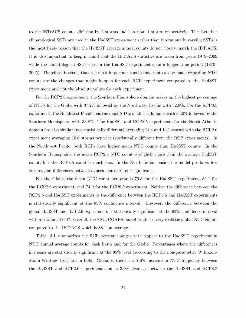
3.2 Normalized average NTC annual counts by basin. Normalization is done respectiveto individual experiments’ average annual global count. Error bars indicate 95%confidence interval. . . . . . . . . . . . . . . . . . . . . . . . . . . . . . . . . . . . . . . 23

3.3 Average NTC duration (days) by basin (error bars indicate 95% confidence interval). 24

3.4 Average NTC annual maximum wind speed (ms−1) by basin (error bars indicate 95%confidence interval). . . . . . . . . . . . . . . . . . . . . . . . . . . . . . . . . . . . . . 25

3.5 Binned 6-hourly maximum wind speeds (ms−1) for all storms’ lifetimes for each ex-periment. Bin size is 2 ms−1. . . . . . . . . . . . . . . . . . . . . . . . . . . . . . . . . 26

3.6 6-hourly maximum wind speed (ms−1) density curves for each experiment. Verticallines represent each experiment’s mean value. . . . . . . . . . . . . . . . . . . . . . . . 27

3.7 Binned storm maximum wind speeds (ms−1) for all storms for each experiment. Binsize is 2 ms−1. . . . . . . . . . . . . . . . . . . . . . . . . . . . . . . . . . . . . . . . . 28

3.8 Storm maximum wind speed (ms−1) density curves for each experiment. Vertical linesrepresent each experiment’s mean value. . . . . . . . . . . . . . . . . . . . . . . . . . . 28

3.9 Binned daily precipitation (mm/day) for all storms’ lifetimes for each experiment. Binsize is 10 mm/day. . . . . . . . . . . . . . . . . . . . . . . . . . . . . . . . . . . . . . . 29

viii

3.10 Daily precipitation (mm/day) density curves for each experiment. Vertical lines rep-resent each experiment’s mean value. . . . . . . . . . . . . . . . . . . . . . . . . . . . . 29

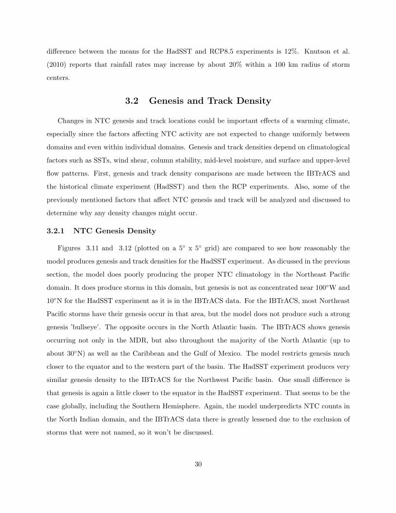
3.11 Genesis density (events/year) for IBTrACS using 5◦ x 5◦ degree grid boxes. . . . . . . 31

3.12 Genesis density (events/year) for HadSST experiment using 5◦ x 5◦ degree grid boxes. 32

3.13 Normalized factoral change in genesis density between the RCP2.6 experiment andthe HadSST experiment using 5◦ x 5◦ degree grid boxes. . . . . . . . . . . . . . . . . . 33

3.14 Normalized factoral change in genesis density between the RCP8.5 experiment andthe HadSST experiment using 5◦ x 5◦ degree grid boxes. . . . . . . . . . . . . . . . . . 33

3.15 Track density (events/year) for IBTrACS using 3◦ x 3◦ degree grid boxes. . . . . . . . 34

3.16 Track density (events/year) for HadSST experiment using 3◦ x 3◦ degree grid boxes . 35

3.17 Normalized factoral change in track density between the RCP2.6 experiment and theHadSST experiment using 3◦ x 3◦ degree grid boxes. . . . . . . . . . . . . . . . . . . . 35

3.18 Normalized factoral change in track density between the RCP8.5 experiment and theHadSST experiment using 3◦ x 3◦ degree grid boxes. . . . . . . . . . . . . . . . . . . . 36

3.19 Global average annual NTC cycle for each model experiment and for IBTrACS (errorbars indicate 95% confidence interval). . . . . . . . . . . . . . . . . . . . . . . . . . . . 37

3.20 North Atlantic average annual NTC cycle for each model experiment and for IBTrACS(error bars indicate 95% confidence interval). . . . . . . . . . . . . . . . . . . . . . . . 37

3.21 Global annual average change in temperature and equivalent potential temperature(θe) (◦C) by pressure level between the RCP2.6 and HadSST experiments (black line)and the RCP8.5 and HadSST experiments (green line). . . . . . . . . . . . . . . . . . 39

3.22 Tropical (30◦S to 30◦N) annual average change in temperature and equivalent potentialtemperature (θe) (◦C) by pressure level between the RCP2.6 and HadSST experiments(black line) and the RCP8.5 and HadSST experiments (green line). . . . . . . . . . . . 40

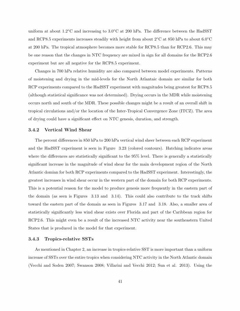
3.23 Percent difference in vertical wind shear (850 hPa to 200 hPa) between the RCP2.6and HadSST experiments and the RCP8.5 and HadSST experiments. Solid contoursare positive differences and perforated contours are negative differences. Hatchingindicates that differences are statisticaly significant at the 95% confidence interval. . . 42

3.24 The June through November mean North Atlantic sea level pressure (hPa) for theHadSST, RCP2.6 and RCP8.5 experiments (a, b, c). The June through Novembermean North Atlantic sea level pressure differences (hPa) between each RCP experi-ment and the HadSST experiment (d, e). . . . . . . . . . . . . . . . . . . . . . . . . . 43

ix

LIST OF ABBREVIATIONS

AGCM Atmospheric General Circulation ModelAMO Atlantic Multi-Decadal OscillationASO August-September-OctoberCCSM4 Community Climate System Model Version 4CMIP5 Fifth Phase of the Climate Model Intercomparison ProjectCOAPS Center for Ocean-Atmospheric Prediction StudiesEPac Northeast PacificFSU Florida State UniversityIBTrACS International Best Track Archive for Climate StewardshipITCZ Inter-Tropical Convergence ZoneMDR Main Development RegionNASH North Atlantic Sub-Tropical HighNAtl North AtlanticNIn North IndianNTC named tropical cyclonePDI Power Dissipation IndexRCP Representative Concentration PathwaySAtl South AtlanticSHem Southern HemisphereSST sea surface temperatureTC tropical cycloneWPac Northwest Pacific

x

ABSTRACT

The effects of two different future warming climate scenarios on global and North Atlantic named

tropical cyclone (NTC) activity is examined using the Florida State University/Center for Ocean-

Atmospheric Prediction Studies (FSU/COAPS) atmospheric general circulation model (AGCM).

The two warming scenarios are based on the Representative Concentration Pathways (RCPs) 2.6

and 8.5 from the Coupled Model Intercomparison Project phase 5 (CMIP5). Previously published

studies show that the FSU/COAPS AGCM has statistically significant skill at reproducing the

observed interannual variability of NTC and hurricane counts in the North Atlantic basin given

observed sea surface temperatures (SSTs). In this study, the FSU/COAPS model is forced with

bias-corrected, monthly-varying, annual climatology SSTs derived from the fourth version of the

Community Climate System Model’s (CCSM4) RCP2.6 and RCP8.5 simulations. In addition, the

FSU/COAPS model’s CO2 concentration is modified to reflect the average CO2 concentration over

the 2006–2100 time period. For each warming experiment, a 14 member ensemble (differing by

initial atmospheric conditions) is made to develop the NTC statistics. In addition, a 14 member

control experiment is performed using observed climatological SSTs from the Hadley Centre. An

objective detection/tracking algorithm is used to identify and track the NTCs from the model

output. For the North Atlantic, a statistically significant increase (14.9%) in the NTC frequency

for the RCP2.6 experiment compared to the control experiment is projected by the model. It is

also found that with increasing SSTs and CO2 concentrations, North Atlantic NTC intensity (as

determined by the NTC maximum 10-meter wind speed) and daily storm-centered precipitation

also increase. NTC genesis is found to move away from regions of increasing vertical wind shear and

decreasing mid-level relative humidity for both future warming climate scenarios. Differences in

the track densities between the warming experiments with the control experiment show an increase

in landfall potential in the Southeast United States.

xi

CHAPTER 1

INTRODUCTION

The overall increase in global temperatures (especially noticeable in sea surface temperatures, or

SSTs) over the late 20th century is a well known fact. Also, raw observational data shows an

increase in tropical cyclone (TC) activity during this period for the North Atlantic basin, and it

has been speculated that global warming might be the cause for these two trends (Webster et

al. 2005). However, the transition from a speculation to a conclusion is complicated by factors

such as internal variability, atmospheric/oceanic dynamics and thermodynamics, teleconnections,

and data integrity. Currently, the exact effect that a warming climate has on TC activity is still

unclear. Fortunately, there are atmospheric models that are able to approximately reproduce the

historical TC climatology in certain basins (from the satellite era forward) using the observed SSTs

from that period. This provides hope that given predicted SSTs for the future climate, those

models that performed well during historical climate estimations can provide reasonable future

climate estimations. The model used in this study has known skill in reproducing historical TC

climatology in the North Atlantic basin using observed SSTs. Thus, by using SSTs from multiple

climate change scenarios, the model is used to estimate potential changes in TC activity as a result

of a warming climate.

1.1 The Predictability of Tropical Cyclone Climatology

1.1.1 Theory

According to the theory of chaos (Lorenz 1963), the smallest possible difference in initial condi-

tions from the actual state of the atmosphere prevents computer models from accurately predicting

conditions beyond about one week, and that is assuming all of the physics and dynamics used in

the model are exactly correct and complete. Since no model is perfect, how could anyone claim to

be able to model the future climate? Large-scale meteorological patterns/circulations vary much

more slowly than local-scale daily conditions and can be more easily predicted relatively far into the

1

future (Shukla 1998). When predictability of these large-scale patterns is dependent on boundary

conditions, such as SSTs, it is called predictability of the second kind.

Large-scale time-mean atmospheric patterns in the tropics, such as rainfall anomalies, are

strongly influenced by slowly changing boundary conditions, such as SSTs (Charney and Shukla

1981). Therefore, if long-term SST patterns could be accurately predicted, then so could the time-

averaged tropical atmospheric patterns. The reasons that this theory holds in the tropics are related

to the shape of the Clausius-Clapeyron curve (which determines the saturation vapor pressure for

a given temperature) and the type of instabilities that are present. The Clausius-Clapeyron curve

has a very steep slope near the range of temperatures which are common for relatively warm SSTs

found in the tropics. Thus, a small change in SSTs leads to a large change in the moisture holding

capacity of the overlying atmosphere and controls large-scale patterns such as rainfall. Additionally,

baroclinic instability is relatively weak in the tropics with weaker horizontal temperature gradients

and less vertical wind shear. Therefore, flow instability does little to affect time-averaged atmo-

spheric patterns, leaving boundary conditions to have the most influence on parameters such as

rainfall anomalies (Shukla 1998). This leads to the question of what other tropical phenomena can

be predicted using boundary conditions. The potential for a model to accurately capture interan-

nual variability in TC activity given observed SSTs has already been shown by various published

studies (Emanuel et al. 2008; Knutson et al. 2008; LaRow et al. 2008; Zhao et al. 2009).

1.1.2 Modeling Tropical Cyclone Climatology

The Florida State University/Center for Ocean-Atmospheric Prediction Studies (FSU/COAPS)

general circulation model (Cocke and LaRow 2000) used by LaRow et al. (2008, 2010) and LaRow

(2013) is used in this study and briefly discussed in Chapter 2. In LaRow et al. (2008), observed

Reynolds OIv2 SSTs were used to force the model and were updated on a weekly basis. Using

these observed SSTs, the FSU/COAPS model had a 0.78 ensemble mean rank correlation for North

Atlantic basin interannual tropical storm variability for the years 1986–2005. Also, in LaRow (2013),

the model was able to reproduce the interannual variability of hurricane counts for the years 1982–

2009 with a mean rank correlation of 0.74. Although this model has shown skill in reproducing the

interannual variability of tropical storms in the North Atlantic, it does not simulate moderate to

intense hurricanes (maximum wind speeds of 45 ms−1 or greater) with the observed frequency. This

is the case for all global models, and the problem results from relatively large model resolutions

2

compared to the scale of internal storm dynamics that enable higher intensities. Some studies have

been performed where model downscaling has been used for regional areas and have been able to

better produce more intense hurricanes (Emanuel et al. 2008; Knutson et al. 2008; Bender et al.

2010; Emanuel 2013). However, the focus of this study is on TC frequnecy and relative intensity

changes between historical conditions and future climate scenarios.

1.2 Environmental Influences on Tropical Cyclone Activity

In order to understand how TC activity will change in future climates, one must know the factors

that lead to or inhibit genesis and that sustain or weaken a storm. The most basic parameters that

enable genesis listed by Gray (1975) are:

1. Adequate low-level relative vorticity

2. Adequate planetary vorticity/coriolis parameter

3. Weak vertical wind shear

4. A deep thermocline with high thermal energy and SSTs being 26◦C or greater

5. Conditional instability up to at least 500 mb

6. High relative humidity through the middle troposphere

The power dissipation index (PDI), which is the integral over the lifetime of the storm of the

maximum surface wind speed raised to the third power, was examined as a proxy for TC activity by

Emanuel (2007). He suggested that future changes in PDI will be dependent on surface radiative

flux, tropopause temperature (impacts storms outflow temperatures), surface wind speed (impacts

heat flux off of the ocean), low-level vorticity, and vertical wind shear. Furthermore, differential

warming in the North Atlantic basin (as compared to tropical mean warming) is suggested to have

a possible relationship with trends in TC activity and PDI (Swanson 2008; Knutson et al. 2010;

Villarini and Vecchi 2012; Zhao and Held 2012; Villarini and Vecchi 2013). This information means

that an expanding 26◦C isotherm does not necessarily mean an expanding area of TC genesis.

Climatological variables such as the ’tropics-relative SST’ will need to be investigated in the model

to help understand why certain changes in TC activity are or are not occurring.

3

1.3 Motivation

Observations suggest that there has been an increase in TC activity (in terms of global intensity

and North Atlantic frequency) over the 20th century (Webster et al. 2005; Vecchi and Knutson

2008), and the roles of climate change (increases in CO2 and other greenhouse gas concentrations

and changes in aerosol concentrations), internal variability, and observational issues have been

questioned as causes for these apparent trends.

Statistical analyses by Mann and Emanuel (2006) and Holland and Webster (2007) have con-

cluded that observed increases in North Atlantic TC numbers over the past 100 years is at least

partially due to anthropogenic forcing toward warmer SSTs. Increases between 0.32◦C and 0.67◦C

over the 20th century for the particularly active North Pacific and North Atlantic basins have been

observed and been statistically shown not to be due entirely to internal variability (Santer et al.

2006). Also, SST data is generally considered accurate (although not as widespread during the

earlier part of that period). Unfortunately, there is a lack of confidence in historical TC activity

data due to multiple observational issues. First, satellite and remote sensing techniques were not

available until the 1960s on, and TC observations were only made by passing ships or as storms

made landfall. Chang and Guo (2007) estimated that TC frequency was underestimated by up to

2.1 TCs per year during the early 20th century. Landsea et al. (2007) and Vecchi and Knutson

(2008) concluded that any positive trend in TC frequency over this period is not statistically sig-

nificant. Furthermore, even if there were a statistically significant trend, one cannot be sure that it

is not due to a possible low-frequency multi-decadal oscillation such as the Atlantic Multi-Decadal

Oscillation (AMO) that cannot be resolved by the relatively short data record (Goldenberg et al.

2001). Since no consensus on the observed trend (or cause of the observed trend) in TC frequency

can be made for the period when global warming is evident using the available data, the effect a

warming climate will have on TC activity remains unclear.

1.4 Results of Similar Research

Many studies have been done to determine the impact that climate change will have on future

TC activity for the Globe and for individual basins using various models and climate change

scenarios. Earlier experiments such as Bengtsson et al. (1996) and Henderson-Sellers et al. (1998)

4

predict that future storms might have the potential to reach stronger intensities. While Henderson-

Sellers et al. (1998) made no solid conclusion about frequency, Bengtsson et al. (1996) predicted a

global reduction in frequency with largest decreases seen in the Southern Hemisphere (possibly due

to reduced low-level relative vorticity and increased vertical wind shear in active hurricane regions).

Later, Bengtsson et al. (2007) explores TC sensitivity to model resolution. They find that their

model at T63 resolution (192 x 96 horizontal grid) predicts a global reduction in frequency of about

20% over the 21st century with no change in intensity. However, their model with T213 resolution

(640 x 320 horizontal grid) predicts a reduction of only 10% with an increase in the number of most

intense storms. They identify that increased static stability related to large-scale tropical circulation

is the cause for the reduction in storm frequency and that the increase in temperature and water

vapor content in the atmosphere contributes to the increase in intense storms. They also support

the idea that tropics-relative SST is most influential on activity (rather than a simple increase in

temperature) because this controls large-scale atmospheric circulations which in turn affect static

stability and TC genesis potential. Zhao et al. (2009) also supports the differential warming theory

in their study which predicts a 15% decrease in frequency for the Atlantic basin, the Northwest

Pacific basin, and the Southern Hemisphere, but a 40% increase in activity in the Northeast Pacific

basin. Held and Zhao (2011) examine the partial effects of increased CO2 concentrations and

increased SSTs on TC frequency and found that each contributed about equally to total a decrease

of about 20%.

Most modeling studies seem to be in agreement that global TC frequency will experience either

little change or a decrease over the 21st century (Knutson et al. 2010). However, Emanuel (2013)

projects an increase in both frequency and intensity of TCs by using a dynamical downscaling tech-

nique and the most recent climate projections. Based on varying results (especially for individual

basins), there is still a necessity for further research on this topic.

1.5 Research Goals

The purpose of this study is to examine and compare data representing the current climate and

various climate warming scenarios and to determine the effect that a warming climate might have

on both global and North Atlantic TC activity. This is done using the FSU/COAPS atmospheric

general circulation model (AGCM) (Cocke and LaRow 2000) which has known skill in predicting

5

interannual TC variability in the current climate (LaRow et al. 2008). The model is forced

with SSTs taken from the 5th phase of the Climate Model Intercomparison Project (CMIP5) as

well as an observed SST dataset. Three different SST sets from the Community Climate System

Model version 4 (CCSM4) respresenting different climatic scenarios are used and compared with

the observed SSTs from the Hadley Centre SST data set. The CCSM4 was chosen since it is one of

the better models within CMIP5 at reproducing historical climate interannual SST variability in

the equatorial Pacific and annual cycle in the North Atlantic region (Stefanova and LaRow 2011;

Liu et al. 2013). The main goals for this research are to:

1. Derive the possible changes in TC activity (frequency, intensity, genesis, etc.) for two different

warming scenarios to be discussed in Chapter 2 and compare the results to similar published

studies

2. Examine potential physical and thermodynamic reasons for the model to produce those

changes

3. Add to the scientific understanding and consensus of climate change and its impacts on

tropical cyclone activity

6

CHAPTER 2

METHOD

This study uses the well-established FSU/COAPS AGCM. This model has previously been shown to

have considerable skill in reproducing the interannual variations in named tropical cyclone (NTC)

activity for the current climate in the North Atlantic basin given observed SSTs (LaRow et al.

2008, 2010; LaRow 2013). Therefore, if given SSTs for future climate scenarios, the expectation

is that the FSU/COAPS model will be able to estimate changes in tropical cyclone activity for

that particular scenario (as compared to the current climate) with some degree of skill. To make

such future climate estimations, two different future climate scenarios (changes in SSTs and CO2

concentrations) are used to force this AGCM. Then, the model output is analyzed to determine

the effect that different climatic warming scenarios might have on NTC activity and environmental

parameters know to affect NTC activity for individual regions and across the Globe.

2.1 Representative Concentration Pathways (RCPs)

The two sets of SSTs representing different future climate scenarios are developed using data

from the CCSM4 which is a general circulation model and is part of CMIP5 (Gent et al. 2011).

The CMIP5 is an organized collaboration between many different climate modeling centers aimed

at examining current climate predictability within models and possible future changes in climate

(Taylor et al. 2012). Within the CMIP5, there are four future climate scenarios that are driven by

different greenhouse gas concentrations. These scenarios are referred to as Representative Concen-

tration Pathways (RCPs), and represent time-varying concentraions of various greenhouse gasses

between the years 2006–2300 (Meinshausen et al. 2011). RCP2.6 and RCP8.5 are the upper and

lower extremes of the four scenarios and their CO2 concentrations for the years 2006–2100 were

used in this study. The suffixes (2.6 and 8.5) refer to the increase in radiative forcing in units of

Wm−2 by the year 2100 compared to the pre-industrial period. Greenhouse gas concentrations for

RCP2.6 correspond to an average surface temperature increase of about 1.5◦C by the year 2100

(compared to the pre-industrial period), and RCP8.5 corresponds to an increase of about 4.5◦C

7

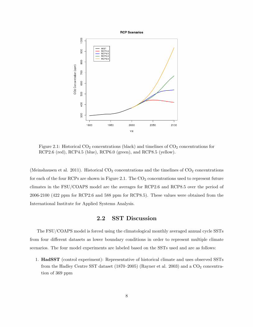
Figure 2.1: Historical CO2 concentrations (black) and timelines of CO2 concentrations forRCP2.6 (red), RCP4.5 (blue), RCP6.0 (green), and RCP8.5 (yellow).

(Meinshausen et al. 2011). Historical CO2 concentrations and the timelines of CO2 concentrations

for each of the four RCPs are shown in Figure 2.1. The CO2 concentrations used to represent future

climates in the FSU/COAPS model are the averages for RCP2.6 and RCP8.5 over the period of

2006-2100 (422 ppm for RCP2.6 and 588 ppm for RCP8.5). These values were obtained from the

International Institute for Applied Systems Analysis.

2.2 SST Discussion

The FSU/COAPS model is forced using the climatological monthly averaged annual cycle SSTs

from four different datasets as lower boundary conditions in order to represent multiple climate

scenarios. The four model experiments are labeled based on the SSTs used and are as follows:

1. HadSST (control experiment): Representative of historical climate and uses observed SSTs

from the Hadley Centre SST dataset (1870–2005) (Rayner et al. 2003) and a CO2 concentra-

tion of 369 ppm

8

2. CCSM4clim: Uses CCSM4 estimation of historical climate SST conditions (1870–2005)

produced from CMIP5 experiment number 3.2 and a CO2 concentration of 369 ppm

3. RCP2.6: Uses bias-corrected CCSM4 SSTs for the RCP2.6 future climate scenario (CMIP5

experiment number 4.3) and a CO2 concentration of 422 ppm

4. RCP8.5: Uses bias-corrected CCSM4 SSTs for the RCP8.5 future climate scenario (CMIP5

experiment number 4.2) and a CO2 concentration of 588 ppm

The SST set used in the HadSST experiment is the climatological annual cycle of monthly

SSTs from the Hadley Centre SST dataset (1870-2005). This experiment is considered the control

experiment since it is the ’baseline’ used to compare the future climate scenario experiments to the

historical climate. As part of CMIP5 experiment number 3.2, the CCSM4 model was run using

historical atmospheric compositions (due to anthropogenic and volcanic activity), solar forcing,

and land use to get its SST estimate for the years 1850–2005 (Taylor et al. 2009; Gent et al.

2011). Only the years 1870–2005 are used for this study to parallel the time period that the Hadley

SSTs are available for. The CCSM4 historical climate SST dataset is used for two reasons. The

first reason is to see how the NTC climatology is represented by the FSU/COAPS model using

the CCSM4’s estimation of non-bias corrected historical SSTs. The climatology of the CCSM4’s

version of current climate SSTs is taken in the same way as previously stated and used to force the

CCSM4clim experiment in the FSU/COAPS model. The second use for the CCSM4’s historical SST

climatology is to determine its bias so that the CCSM4’s estimation of SSTs in the future climate

scenarios can be bias-corrected before averaging them and using them to force the FSU/COAPS

model. In order to determine the model’s ability to reproduce the historical climate using observed

CO2 concentrations, and therefore the model bias, the SSTs from the CCSM4’s historical climate

experiment were compared to the observed Hadley SST dataset. The difference between the two

provides the model bias and is later used to correct the CCSM4’s SSTs for future climate scenarios.

Equations 2.1 and 2.2 represent the development and use of the CCSM4’s SST bias. The annual

climatology by month is taken for the model bias.

F∗ = F − (H −O) (2.1)

F∗ = O + (F −H) = O + ∆RCP (2.2)

where,

9

F: CCSM4 future projected SSTs (based on RCPs)

H: CCSM4 estimation of historical SSTs

O: Observed historical SSTs (Hadley Centre)

x: Monthly climatology is taken

*: Bias-corrected

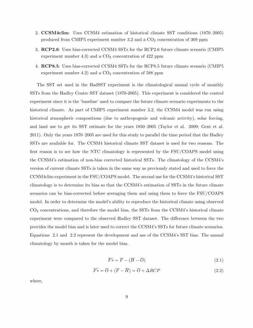
Figure 2.2 shows the total time-averaged CCSM4 bias, and Figure 2.3 shows the August-

September-October (ASO) averaged CCSM4 bias which is most important for the North Atlantic

basin. It is important to note that when using any SST climatology to force the FSU/COAPS

model, all interannual variability of SSTs (El Nino and La Nina events for example) is removed.

Also, the effect of sea ice temperatures on TC activity in the model is not fully understood in this

study but is estimated to be small (Zhao et al. 2009).

In the equatorial Pacific, there is generally a cool bias of up to 0.5◦C when annually averaged.

However, when comparing the annual bias in this area to the ASO season bias, the magnitude of

the cool bias increases by around 0.5◦C. This demonstrates how important it is to remove the bias

month by month in order to accurately represent SSTs during the peak tropical cyclone season

for each basin. There is also a noticeable cold bias in the Northwest Pacific which increases in

magnitude by about 1◦C during the ASO season. Also in the Pacific, there are warm biases

apparent for both the yearly averaged and ASO averaged plots near the coasts of North and South

America. There is generally a cold bias in the Gulf of Mexico and the Main Development Region

(MDR) of the North Atlantic basin (10◦N to 20◦N and 20◦W to 80◦W). Again the magnitudes of

the cold biases seem to amplify during the ASO season compared to the annual average. Gent et

al. (2011) indicate that the cold bias in this region is due to the CCSM4 still having an issue with

the location of the Gulf Stream which is not thoroughly examined in this study. In the equatorial

Indian Ocean, there is a warm bias off of the west coast of Australia. Both of these biases are

stronger in the ASO season than in the annual average. Although these biases are removed from

the SSTs used to force the FSU/COAPS model, they are non-trivial in some regions (especially

near the Gulf Stream in the North Atlantic) and should be kept in mind.

The two remaining SST datasets (used in the RCP2.6 and RCP8.5 experiments) are also derived

from CMIP5 experiments using the CCSM4 model. The CCSM4 estimations of the SSTs for these

10

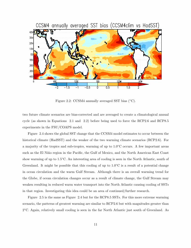
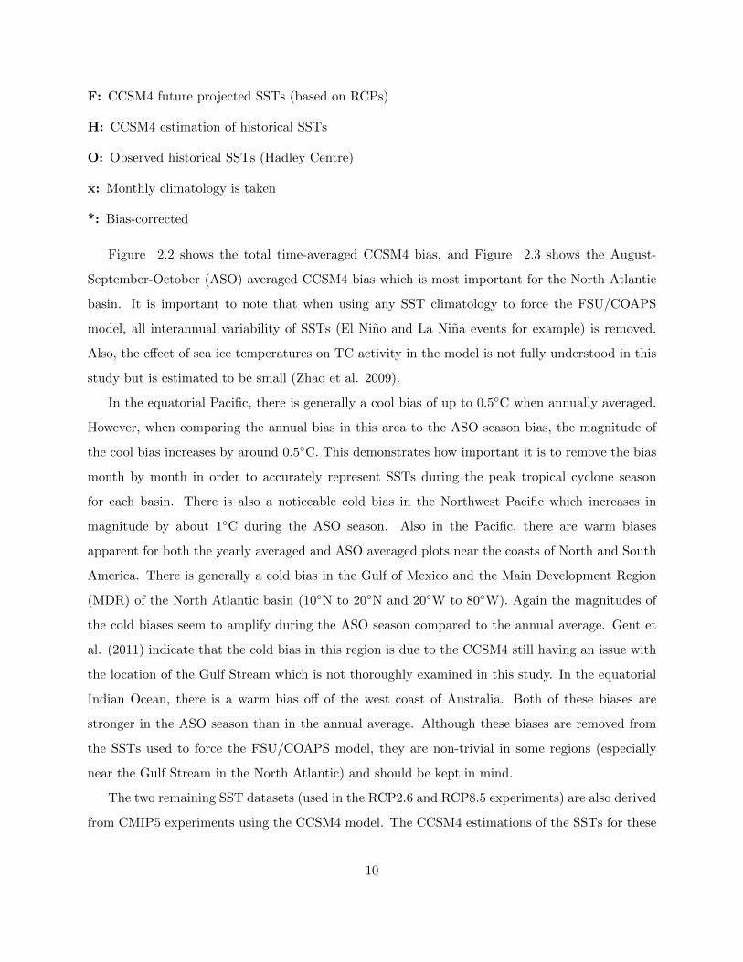
Figure 2.2: CCSM4 annually averaged SST bias (◦C).

two future climate scenarios are bias-corrected and are averaged to create a climatological annual

cycle (as shown in Equations 2.1 and 2.2) before being used to force the RCP2.6 and RCP8.5

experiments in the FSU/COAPS model.

Figure 2.4 shows the global SST change that the CCSM4 model estimates to occur between the

historical climate (HadSST) and the weaker of the two warming climate scenarios (RCP2.6). For

a majority of the tropics and sub-tropics, warming of up to 1.0◦C occurs. A few important areas

such as the El Nino region in the Pacific, the Gulf of Mexico, and the North American East Coast

show warming of up to 1.5◦C. An interesting area of cooling is seen in the North Atlantic, south of

Greenland. It might be possible that this cooling of up to 1.0◦C is a result of a potential change

in ocean circulation and the warm Gulf Stream. Although there is an overall warming trend for

the Globe, if ocean circulation changes occur as a result of climate change, the Gulf Stream may

weaken resulting in reduced warm water transport into the North Atlantic causing cooling of SSTs

in that region. Investigating this idea could be an area of continued/further research.

Figure 2.5 is the same as Figure 2.4 but for the RCP8.5 SSTs. For this more extreme warming

scenario, the patterns of greatest warming are similar to RCP2.6 but with magnitudes greater than

2◦C. Again, relatively small cooling is seen in the far North Atlantic just south of Greenland. As

11

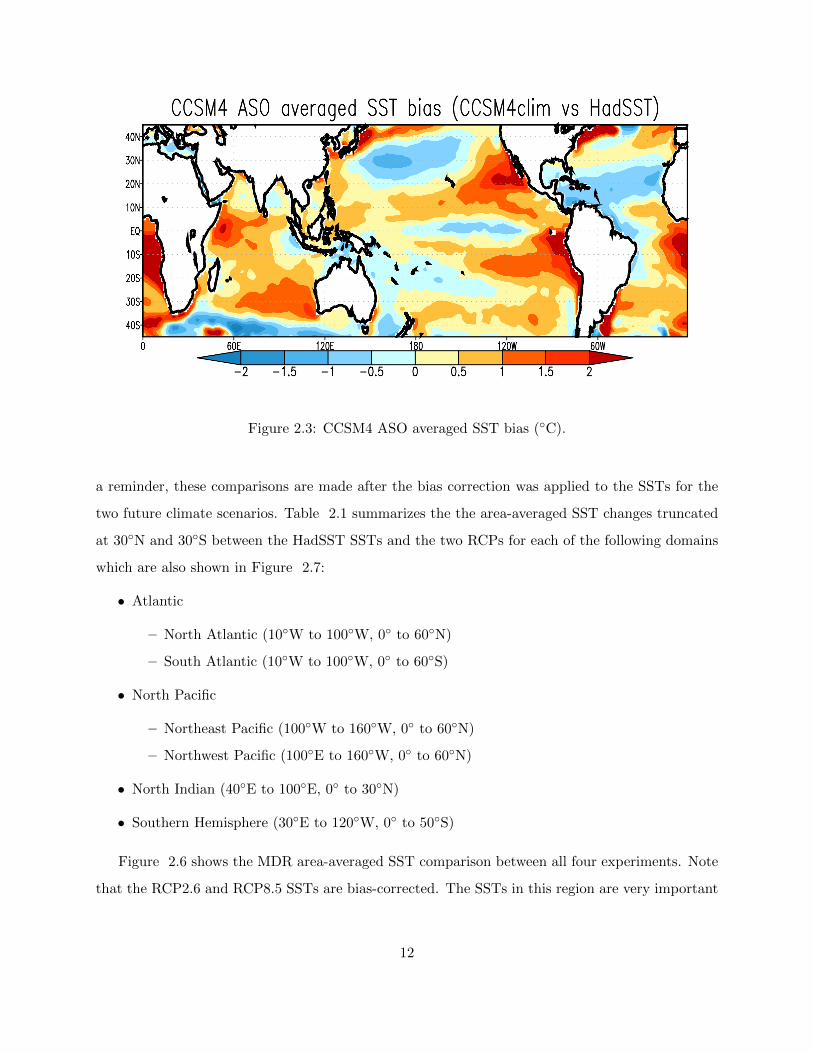
Figure 2.3: CCSM4 ASO averaged SST bias (◦C).

a reminder, these comparisons are made after the bias correction was applied to the SSTs for the

two future climate scenarios. Table 2.1 summarizes the the area-averaged SST changes truncated

at 30◦N and 30◦S between the HadSST SSTs and the two RCPs for each of the following domains

which are also shown in Figure 2.7:

• Atlantic

– North Atlantic (10◦W to 100◦W, 0◦ to 60◦N)

– South Atlantic (10◦W to 100◦W, 0◦ to 60◦S)

• North Pacific

– Northeast Pacific (100◦W to 160◦W, 0◦ to 60◦N)

– Northwest Pacific (100◦E to 160◦W, 0◦ to 60◦N)

• North Indian (40◦E to 100◦E, 0◦ to 30◦N)

• Southern Hemisphere (30◦E to 120◦W, 0◦ to 50◦S)

Figure 2.6 shows the MDR area-averaged SST comparison between all four experiments. Note

that the RCP2.6 and RCP8.5 SSTs are bias-corrected. The SSTs in this region are very important

12

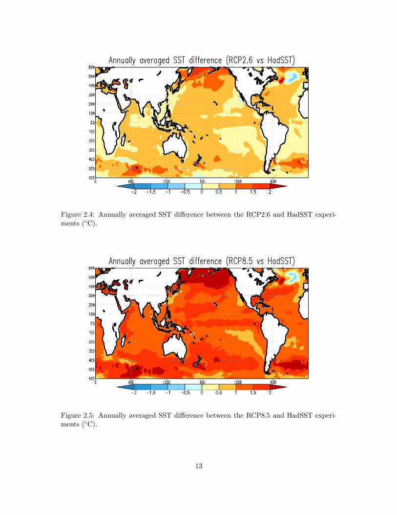
Figure 2.4: Annually averaged SST difference between the RCP2.6 and HadSST experi-ments (◦C).

Figure 2.5: Annually averaged SST difference between the RCP8.5 and HadSST experi-ments (◦C).

13

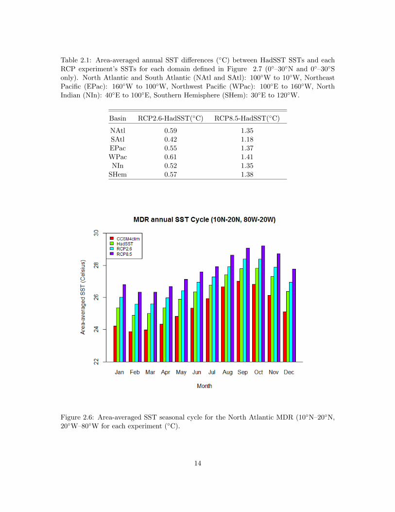
Table 2.1: Area-averaged annual SST differences (◦C) between HadSST SSTs and eachRCP experiment’s SSTs for each domain defined in Figure 2.7 (0◦–30◦N and 0◦–30◦Sonly). North Atlantic and South Atlantic (NAtl and SAtl): 100◦W to 10◦W, NortheastPacific (EPac): 160◦W to 100◦W, Northwest Pacific (WPac): 100◦E to 160◦W, NorthIndian (NIn): 40◦E to 100◦E, Southern Hemisphere (SHem): 30◦E to 120◦W.

Basin RCP2.6-HadSST(◦C) RCP8.5-HadSST(◦C)

NAtl 0.59 1.35SAtl 0.42 1.18EPac 0.55 1.37WPac 0.61 1.41NIn 0.52 1.35

SHem 0.57 1.38

Figure 2.6: Area-averaged SST seasonal cycle for the North Atlantic MDR (10◦N–20◦N,20◦W–80◦W for each experiment (◦C).

14

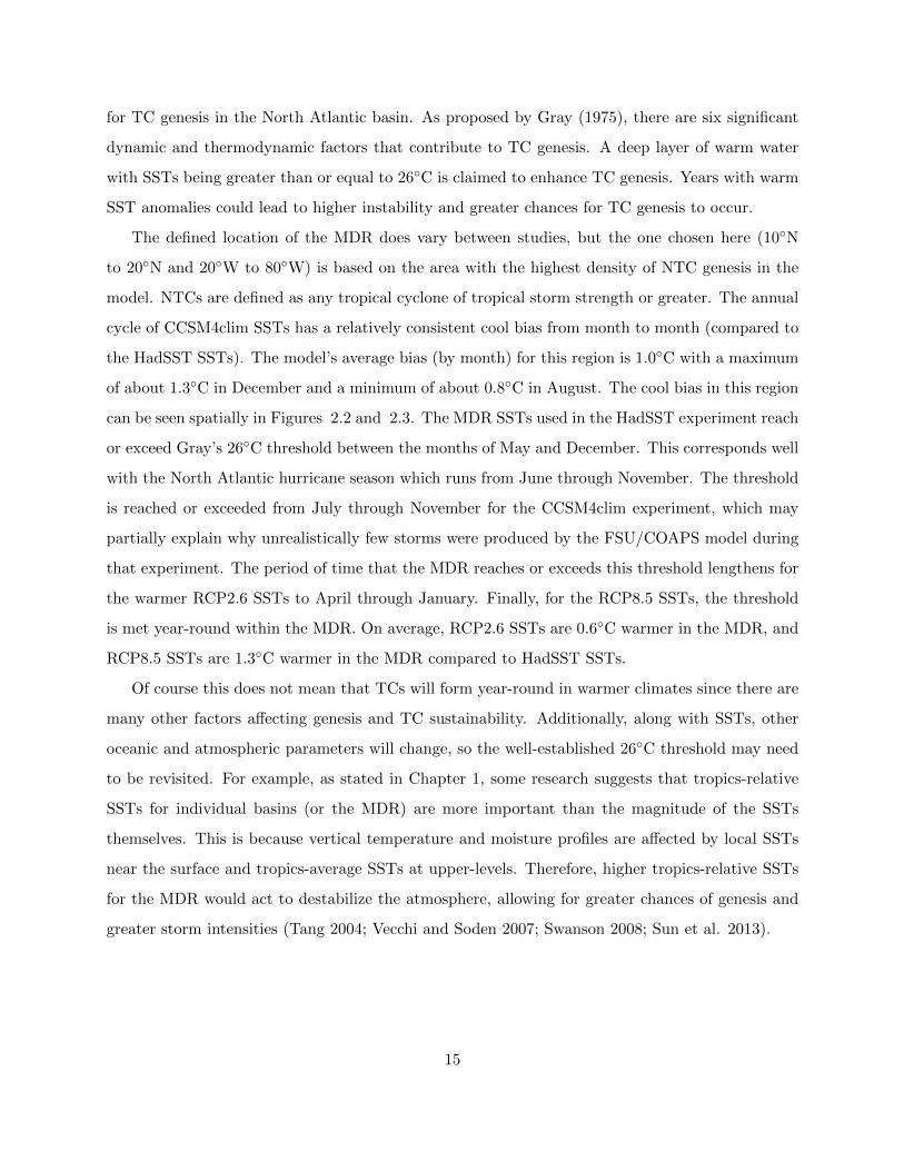
for TC genesis in the North Atlantic basin. As proposed by Gray (1975), there are six significant

dynamic and thermodynamic factors that contribute to TC genesis. A deep layer of warm water

with SSTs being greater than or equal to 26◦C is claimed to enhance TC genesis. Years with warm

SST anomalies could lead to higher instability and greater chances for TC genesis to occur.

The defined location of the MDR does vary between studies, but the one chosen here (10◦N

to 20◦N and 20◦W to 80◦W) is based on the area with the highest density of NTC genesis in the

model. NTCs are defined as any tropical cyclone of tropical storm strength or greater. The annual

cycle of CCSM4clim SSTs has a relatively consistent cool bias from month to month (compared to

the HadSST SSTs). The model’s average bias (by month) for this region is 1.0◦C with a maximum

of about 1.3◦C in December and a minimum of about 0.8◦C in August. The cool bias in this region

can be seen spatially in Figures 2.2 and 2.3. The MDR SSTs used in the HadSST experiment reach

or exceed Gray’s 26◦C threshold between the months of May and December. This corresponds well

with the North Atlantic hurricane season which runs from June through November. The threshold

is reached or exceeded from July through November for the CCSM4clim experiment, which may

partially explain why unrealistically few storms were produced by the FSU/COAPS model during

that experiment. The period of time that the MDR reaches or exceeds this threshold lengthens for

the warmer RCP2.6 SSTs to April through January. Finally, for the RCP8.5 SSTs, the threshold

is met year-round within the MDR. On average, RCP2.6 SSTs are 0.6◦C warmer in the MDR, and

RCP8.5 SSTs are 1.3◦C warmer in the MDR compared to HadSST SSTs.

Of course this does not mean that TCs will form year-round in warmer climates since there are

many other factors affecting genesis and TC sustainability. Additionally, along with SSTs, other

oceanic and atmospheric parameters will change, so the well-established 26◦C threshold may need

to be revisited. For example, as stated in Chapter 1, some research suggests that tropics-relative

SSTs for individual basins (or the MDR) are more important than the magnitude of the SSTs

themselves. This is because vertical temperature and moisture profiles are affected by local SSTs

near the surface and tropics-average SSTs at upper-levels. Therefore, higher tropics-relative SSTs

for the MDR would act to destabilize the atmosphere, allowing for greater chances of genesis and

greater storm intensities (Tang 2004; Vecchi and Soden 2007; Swanson 2008; Sun et al. 2013).

15

2.3 Experiment Design

The FSU/COAPS model has a resolution of T126L27 (about 0.9◦x0.9◦ with 27 vertical levels).

This model has already demonstrated skill in producing realistic tropical storm durations and

reproducing the interannual variability of hurricane frequency having a correlation of 0.74 using

weekly observed SSTs for the years 1982–2009 (LaRow 2013).

Four experiments (HadSST, CCSM4clim, RCP2.6 and RCP8.5) are performed in order to ex-

amine how changes in SSTs and CO2 concentrations affect NTC activity. Fourteen integrations

(using different January 1st initial conditions) were performed for each of the four experiments.

The HadSST and CCSM4clim experiments were forced with their respective monthly SST sets

(as described in the previous section). In these two experiments, the CO2 concentration is set at

369 ppm. The RCP2.6 and RCP8.5 experiments were forced with their respective bias-corrected

monthly SST sets and their average CO2 concentrations from the years 2006-2100 (as described

above).

The same NTC objective detection/tracking algorithm used in LaRow et al. (2008, 2010) and

LaRow (2013) is used for this study with minor modifications. The criteria to count and track a

storm are as follows:

• First, the algorithm must detect a local vorticity maximum of greater than 1 x 10−4 s−1 at

850 hPa.

• Then, it locates the minimum sea level pressure within a 2◦ radius of the local vorticity

maximum.

• Next, the local maximum temperature anomaly between 500 and 200 hPa found within a

2◦ radius from the defined storm center must be at least 3◦C warmer than the surrounding

mean.

• Also, a minimum wind speed of 15 ms−1 must be detected within a 4◦ radius of the storm

center. Initially, the minimum wind speed was set at 17 ms−1 but was lowered based on

relatively coarse model resolution and limited ability to resolve the strongest storms (Walsh

et al. 2007).

• Finally, the conditions above must be met to produce a storm trajectory that lasts for at

least 2 days.

16

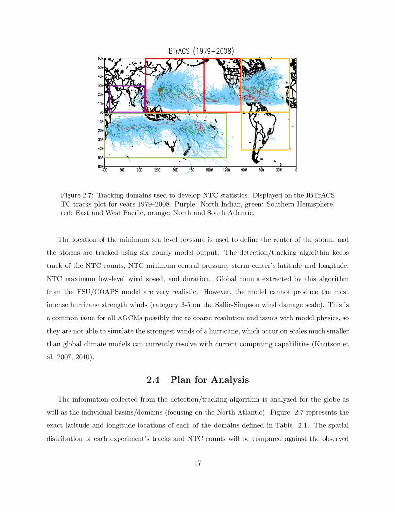
Figure 2.7: Tracking domains used to develop NTC statistics. Displayed on the IBTrACSTC tracks plot for years 1979–2008. Purple: North Indian, green: Southern Hemisphere,red: East and West Pacific, orange: North and South Atlantic.

The location of the minimum sea level pressure is used to define the center of the storm, and

the storms are tracked using six hourly model output. The detection/tracking algorithm keeps

track of the NTC counts, NTC minimum central pressure, storm center’s latitude and longitude,

NTC maximum low-level wind speed, and duration. Global counts extracted by this algorithm

from the FSU/COAPS model are very realistic. However, the model cannot produce the most

intense hurricane strength winds (category 3-5 on the Saffir-Simpson wind damage scale). This is

a common issue for all AGCMs possibly due to coarse resolution and issues with model physics, so

they are not able to simulate the strongest winds of a hurricane, which occur on scales much smaller

than global climate models can currently resolve with current computing capabilities (Knutson et

al. 2007, 2010).

2.4 Plan for Analysis

The information collected from the detection/tracking algorithm is analyzed for the globe as

well as the individual basins/domains (focusing on the North Atlantic). Figure 2.7 represents the

exact latitude and longitude locations of each of the domains defined in Table 2.1. The spatial

distribution of each experiment’s tracks and NTC counts will be compared against the observed

17

International Best Track Archive for Climate Stewardship (IBTrACS ) data (Knapp et al. 2010).

Differences in counts, wind speeds, precipitation, and locations of genesis and tracks between the

experiments are examined for the Globe and for individual domains, focusing on the North Atlantic.

Then, once those statistics have been completed, analysis on other parameters that are derived from

the model output will be performed in order to offer explanations as to why any changes occur.

Parameters such as North Atlantic sea level pressure patterns, mid-level relative humidity, vertical

wind shear, static stability, and tropics-relative SSTs are examined.

18

CHAPTER 3

RESULTS AND DISCUSSION

Information gathered from the detection/tracking algorithm is used to develop NTC statistics for

each model experiment to be compared to each other and to the IBTrACS. Differences in NTC

counts, durations, wind speeds, precipitation, and genesis and track densities between experiments

are examined for statistical significance in each domain. Then, climatological changes in other

parameters such as temperature and equivalent potential temperature profiles, relative humidity,

vertical wind shear, sea level pressure patterns, and tropics-relative SST are examined in the North

Atlantic domain in an effort to explain some of the changes in NTC statistics.

3.1 NTC Statistics by Domain

A warming climate may not have the same effect on NTCs everywhere on the Globe (Knutson et

al. 2010). As shown in Chapter 2, SST changes are not uniform across all basins, so neither should

other factors affecting NTC statistics such as vertical wind shear and mid-level relative humidity.

Parameters like these will be examined and discussed later in Chapter 3. Here, NTC statistics of

count, duration, wind speed, and precipitation for each model experiment (and the IBTrACS) will

be compared and contrasted by basin with focus on the North Atlantic.

3.1.1 NTC Counts

Figure 3.1 shows the histogram of the ensemble average NTC count per year for each exper-

iment and for the IBTrACS by basin with the 95% confidence intervals represented by error bars

using standard error. This assumes that the full range of variability is captured by the 14 ensemble

members. Ideally, there could be at least double the number of ensemble members for each experi-

ment to increase sample size, but ensemble size (and sample size) is limited for this study based on

time and computing resources. For each domain plotted along the x-axis, the model experiments

are plotted left to right by increasing SSTs. It is important to note that the counting algorithm

19

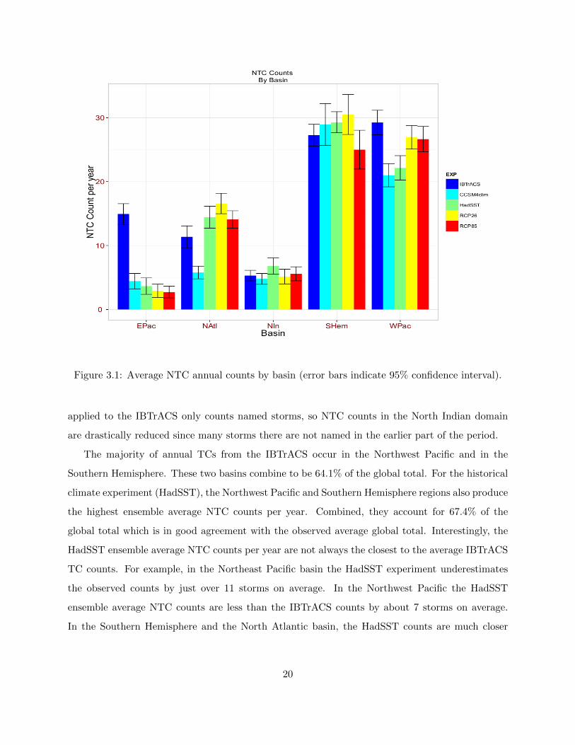
Figure 3.1: Average NTC annual counts by basin (error bars indicate 95% confidence interval).

applied to the IBTrACS only counts named storms, so NTC counts in the North Indian domain

are drastically reduced since many storms there are not named in the earlier part of the period.

The majority of annual TCs from the IBTrACS occur in the Northwest Pacific and in the

Southern Hemisphere. These two basins combine to be 64.1% of the global total. For the historical

climate experiment (HadSST), the Northwest Pacific and Southern Hemisphere regions also produce

the highest ensemble average NTC counts per year. Combined, they account for 67.4% of the

global total which is in good agreement with the observed average global total. Interestingly, the

HadSST ensemble average NTC counts per year are not always the closest to the average IBTrACS

TC counts. For example, in the Northeast Pacific basin the HadSST experiment underestimates

the observed counts by just over 11 storms on average. In the Northwest Pacific the HadSST

ensemble average NTC counts are less than the IBTrACS counts by about 7 storms on average.

In the Southern Hemisphere and the North Atlantic basin, the HadSST counts are much closer

20

to the IBTrACS counts, differing by 2 storms and less than 1 storm, respectively. The fact that

climatological SSTs are used in the HadSST experiment rather than interannually varying SSTs is

the most likely reason that the HadSST average annual counts do not closely match the IBTrACS.

It is also important to keep in mind that the IBTrACS statistics are taken from years 1979–2009

while the climatological SSTs used in the HadSST experiment span a longer time period (1870–

2005). Therefore, it seems that the most important conclusions that can be made regarding NTC

counts are the changes that might happen for each RCP experiment compared to the HadSST

experiment and not the absolute values for each experiment.

For the RCP2.6 experiment, the Southern Hemisphere domain makes up the highest percentage

of NTCs for the Globe with 37.2% followed by the Northwest Pacific with 32.8%. For the RCP8.5

experiment, the Northwest Pacific has the most NTCs of all the domains with 36.0% followed by the

Southern Hemisphere with 33.8%. The HadSST and RCP8.5 experiments for the North Atlantic

domain are also similar (not statistically different) averaging 14.4 and 14.1 storms with the RCP2.6

experiment averaging 16.6 storms per year (statistically different from the RCP experiments). In

the Northwest Pacifc, both RCPs have higher mean NTC counts than HadSST counts. In the

Southern Hemisphere, the mean RCP2.6 NTC count is slightly more than the average HadSST

count, but the RCP8.5 count is much less. In the North Indian basin, the model produces few

storms, and differences between experimentss are not significant.

For the Globe, the mean NTC count per year is 76.3 for the HadSST experiment, 82.1 for

the RCP2.6 experiment, and 74.0 for the RCP8.5 experiment. Neither the difference between the

RCP2.6 and HadSST experiments or the difference between the RCP8.5 and HadSST experiments

is statistically significant at the 95% confidence interval. However, the difference between the

global HadSST and RCP2.6 experiments is statistically significant at the 93% confidence interval

with a p-value of 0.07. Overall, the FSU/COAPS model produces very realistic global NTC counts

compared to the IBTrACS which is 88.1 on average.

Table 3.1 summarizes the RCP percent changes with respect to the HadSST experiment in

NTC annual average counts for each basin and for the Globe. Percentages where the differences

in means are statistically significant at the 95% level (according to the non-parametric Wilcoxon-

Mann-Whitney test) are in bold. Globally, there is a 7.6% increase in NTC frequency between

the HadSST and RCP2.6 experiments and a 3.0% decrease between the HadSST and RCP8.5

21

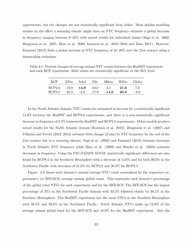
experiments, but the changes are not statistically significant from either. Most similar modeling

studies on the effect a warming climate might have on NTC frequency estimate a global decrease

in frequency ranging between 6–34% with mixed results for individual basins (Sugi et al. 2002;

Bengtsson et al. 2007; Zhao et al. 2009; Knutson et al. 2010; Held and Zhao 2011). However,

Emanuel (2013) finds a global increase in NTC frequency of 10–40% over the 21st century using a

downscaling technique.

Table 3.1: Percent changes of average annual NTC counts between the HadSST experimentand each RCP experiment. Bold values are statistically significant at the 95% level.

RCP EPac NAtl NIn SHem WPac Globe

RCP2.6 -19.8 14.9 -24.0 4.1 21.6 7.6RCP8.5 -25.5 -2.5 -17.9 −14.6 20.3 -3.0

In the North Atlantic domain, NTC counts are estimated to increase by a statistically significant

14.9% between the HadSST and RCP2.6 experiments, and there is a non-statistically significant

decrease in frequency of 2.5% between the HadSST and RCP8.5 experiments. Other models produce

mixed results for the North Atlantic domain (Knutson et al. 2010). Bengtsson et al. (2007) and

Villarini and Vecchi (2012, 2013) estimate little change (if any) in NTC frequency by the end of the

21st century due to a warming climate. Sugi et al. (2002) and Emanuel (2013) estimate increases

in North Atlantic NTC frequency while Zhao et al. (2009) and Bender et al. (2010) estimate

decreases in frequency. Using the FSU/COAPS AGCM, statistically significant differences are also

found for RCP8.5 in the Southern Hemisphere with a decrease of 14.6% and for both RCPs in the

Northwest Pacific with increases of 21.6% for RCP2.6 and 20.3% for RCP8.5.

Figure 3.2 shows each domain’s annual average NTC count normalized by the respective ex-

periment’s (or IBTrACS) average annual global count. This represents each domain’s percentage

of the global total NTCs for each experiment and for the IBTrACS. The IBTrACS has the largest

percentage of TCs in the Northwest Pacific domain with 33.2% followed closely by 30.1% in the

Southern Hemisphere. The HadSST experiment has the most NTCs in the Southern Hemisphere

with 38.4% and 29.0% in the Northwest Pacific. North Atlantic NTCs make up 12.9% of the

average annual global total for the IBTrACS and 18.9% for the HadSST experiment. Also the

22

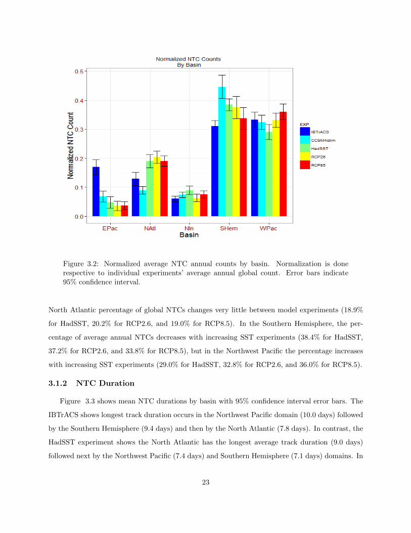
Figure 3.2: Normalized average NTC annual counts by basin. Normalization is donerespective to individual experiments’ average annual global count. Error bars indicate95% confidence interval.

North Atlantic percentage of global NTCs changes very little between model experiments (18.9%

for HadSST, 20.2% for RCP2.6, and 19.0% for RCP8.5). In the Southern Hemisphere, the per-

centage of average annual NTCs decreases with increasing SST experiments (38.4% for HadSST,

37.2% for RCP2.6, and 33.8% for RCP8.5), but in the Northwest Pacific the percentage increases

with increasing SST experiments (29.0% for HadSST, 32.8% for RCP2.6, and 36.0% for RCP8.5).

3.1.2 NTC Duration

Figure 3.3 shows mean NTC durations by basin with 95% confidence interval error bars. The

IBTrACS shows longest track duration occurs in the Northwest Pacific domain (10.0 days) followed

by the Southern Hemisphere (9.4 days) and then by the North Atlantic (7.8 days). In contrast, the

HadSST experiment shows the North Atlantic has the longest average track duration (9.0 days)

followed next by the Northwest Pacific (7.4 days) and Southern Hemisphere (7.1 days) domains. In

23

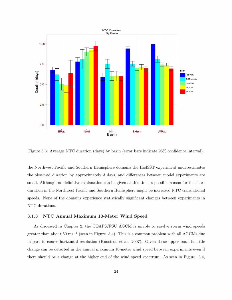
Figure 3.3: Average NTC duration (days) by basin (error bars indicate 95% confidence interval).

the Northwest Pacific and Southern Hemisphere domains the HadSST experiment underestimates

the observed duration by approximately 3 days, and differences between model experiments are

small. Although no definitive explanation can be given at this time, a possible reason for the short

duration in the Northwest Pacific and Southern Hemisphere might be increased NTC translational

speeds. None of the domains experience statistically significant changes between experiments in

NTC durations.

3.1.3 NTC Annual Maximum 10-Meter Wind Speed

As discussed in Chapter 2, the COAPS/FSU AGCM is unable to resolve storm wind speeds

greater than about 50 ms−1 (seen in Figure 3.4). This is a common problem with all AGCMs due

in part to coarse horizontal resolution (Knustson et al. 2007). Given these upper bounds, little

change can be detected in the annual maximum 10-meter wind speed between experiments even if

there should be a change at the higher end of the wind speed spectrum. As seen in Figure 3.4,

24

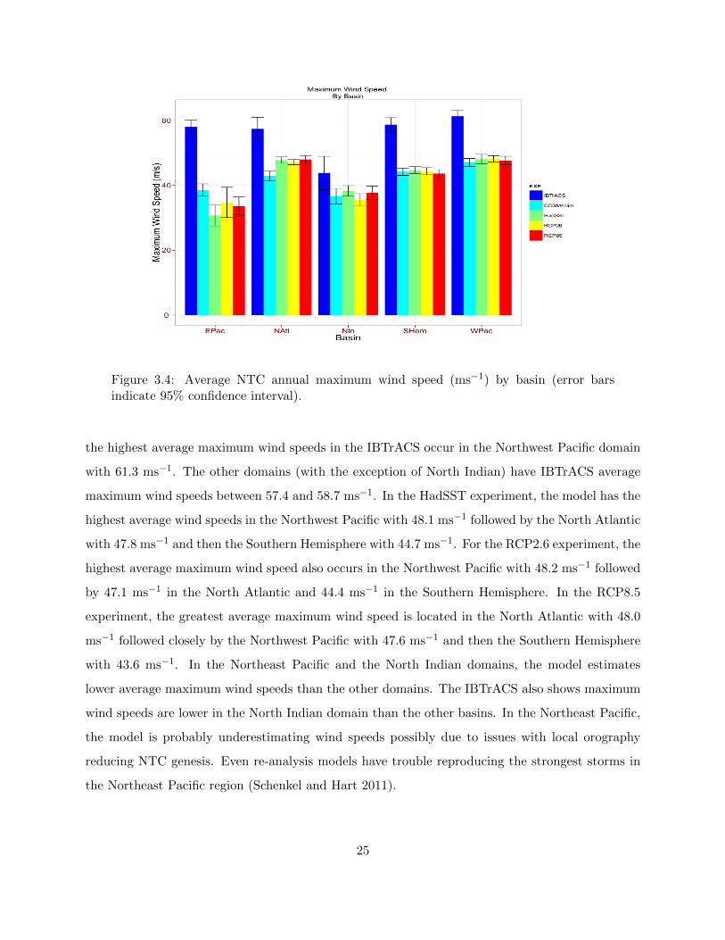
Figure 3.4: Average NTC annual maximum wind speed (ms−1) by basin (error barsindicate 95% confidence interval).

the highest average maximum wind speeds in the IBTrACS occur in the Northwest Pacific domain

with 61.3 ms−1. The other domains (with the exception of North Indian) have IBTrACS average

maximum wind speeds between 57.4 and 58.7 ms−1. In the HadSST experiment, the model has the

highest average wind speeds in the Northwest Pacific with 48.1 ms−1 followed by the North Atlantic

with 47.8 ms−1 and then the Southern Hemisphere with 44.7 ms−1. For the RCP2.6 experiment, the

highest average maximum wind speed also occurs in the Northwest Pacific with 48.2 ms−1 followed

by 47.1 ms−1 in the North Atlantic and 44.4 ms−1 in the Southern Hemisphere. In the RCP8.5

experiment, the greatest average maximum wind speed is located in the North Atlantic with 48.0

ms−1 followed closely by the Northwest Pacific with 47.6 ms−1 and then the Southern Hemisphere

with 43.6 ms−1. In the Northeast Pacific and the North Indian domains, the model estimates

lower average maximum wind speeds than the other domains. The IBTrACS also shows maximum

wind speeds are lower in the North Indian domain than the other basins. In the Northeast Pacific,

the model is probably underestimating wind speeds possibly due to issues with local orography

reducing NTC genesis. Even re-analysis models have trouble reproducing the strongest storms in

the Northeast Pacific region (Schenkel and Hart 2011).

25

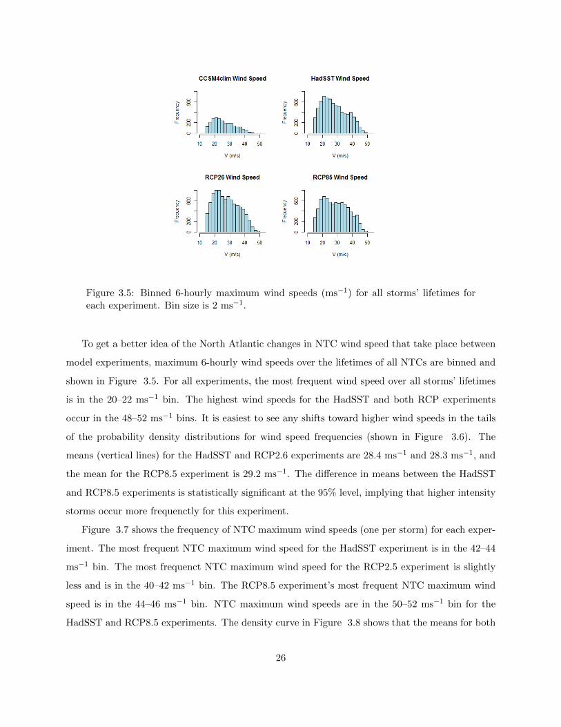
Figure 3.5: Binned 6-hourly maximum wind speeds (ms−1) for all storms’ lifetimes foreach experiment. Bin size is 2 ms−1.

To get a better idea of the North Atlantic changes in NTC wind speed that take place between

model experiments, maximum 6-hourly wind speeds over the lifetimes of all NTCs are binned and

shown in Figure 3.5. For all experiments, the most frequent wind speed over all storms’ lifetimes

is in the 20–22 ms−1 bin. The highest wind speeds for the HadSST and both RCP experiments

occur in the 48–52 ms−1 bins. It is easiest to see any shifts toward higher wind speeds in the tails

of the probability density distributions for wind speed frequencies (shown in Figure 3.6). The

means (vertical lines) for the HadSST and RCP2.6 experiments are 28.4 ms−1 and 28.3 ms−1, and

the mean for the RCP8.5 experiment is 29.2 ms−1. The difference in means between the HadSST

and RCP8.5 experiments is statistically significant at the 95% level, implying that higher intensity

storms occur more frequenctly for this experiment.

Figure 3.7 shows the frequency of NTC maximum wind speeds (one per storm) for each exper-

iment. The most frequent NTC maximum wind speed for the HadSST experiment is in the 42–44

ms−1 bin. The most frequenct NTC maximum wind speed for the RCP2.5 experiment is slightly

less and is in the 40–42 ms−1 bin. The RCP8.5 experiment’s most frequent NTC maximum wind

speed is in the 44–46 ms−1 bin. NTC maximum wind speeds are in the 50–52 ms−1 bin for the

HadSST and RCP8.5 experiments. The density curve in Figure 3.8 shows that the means for both

26

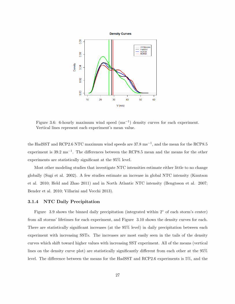
Figure 3.6: 6-hourly maximum wind speed (ms−1) density curves for each experiment.Vertical lines represent each experiment’s mean value.

the HadSST and RCP2.6 NTC maximum wind speeds are 37.8 ms−1, and the mean for the RCP8.5

experiment is 39.2 ms−1. The differences between the RCP8.5 mean and the means for the other

experiments are statistically significant at the 95% level.

Most other modeling studies that investigate NTC intensities estimate either little to no change

globally (Sugi et al. 2002). A few studies estimate an increase in global NTC intensity (Knutson

et al. 2010; Held and Zhao 2011) and in North Atlantic NTC intensity (Bengtsson et al. 2007;

Bender et al. 2010; Villarini and Vecchi 2013).

3.1.4 NTC Daily Precipitation

Figure 3.9 shows the binned daily precipitation (integrated within 2◦ of each storm’s center)

from all storms’ lifetimes for each experiment, and Figure 3.10 shows the density curves for each.

There are statistically significant increases (at the 95% level) in daily precipitation between each

experiment with increasing SSTs. The increases are most easily seen in the tails of the density

curves which shift toward higher values with increasing SST experiment. All of the means (vertical

lines on the density curve plot) are statistically significantly different from each other at the 95%

level. The difference between the means for the HadSST and RCP2.6 experiments is 5%, and the

27

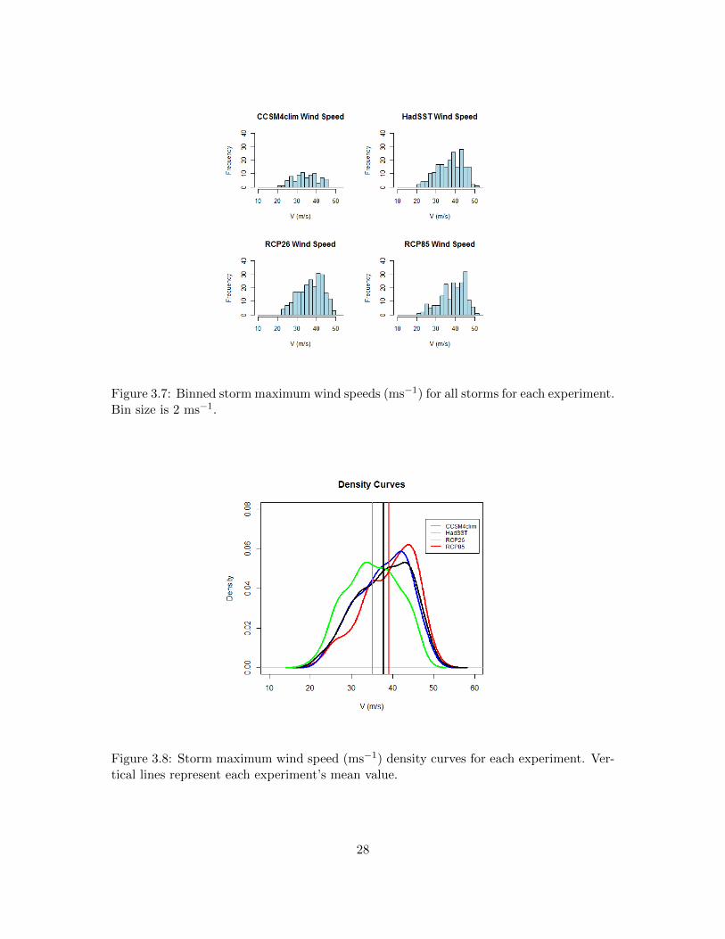
Figure 3.7: Binned storm maximum wind speeds (ms−1) for all storms for each experiment.Bin size is 2 ms−1.

Figure 3.8: Storm maximum wind speed (ms−1) density curves for each experiment. Ver-tical lines represent each experiment’s mean value.

28

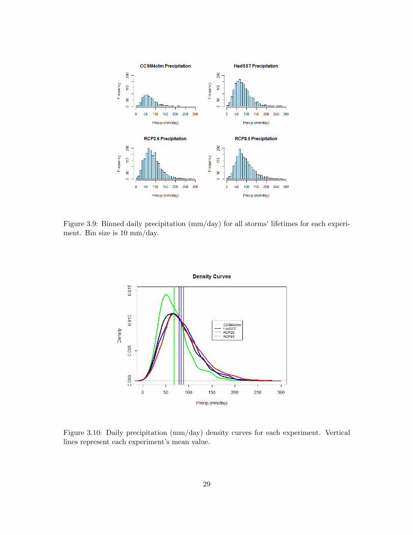
Figure 3.9: Binned daily precipitation (mm/day) for all storms’ lifetimes for each experi-ment. Bin size is 10 mm/day.

Figure 3.10: Daily precipitation (mm/day) density curves for each experiment. Verticallines represent each experiment’s mean value.

29

difference between the means for the HadSST and RCP8.5 experiments is 12%. Knutson et al.

(2010) reports that rainfall rates may increase by about 20% within a 100 km radius of storm

centers.

3.2 Genesis and Track Density

Changes in NTC genesis and track locations could be important effects of a warming climate,

especially since the factors affecting NTC activity are not expected to change uniformly between

domains and even within individual domains. Genesis and track densities depend on climatological

factors such as SSTs, wind shear, column stability, mid-level moisture, and surface and upper-level

flow patterns. First, genesis and track density comparisons are made between the IBTrACS and

the historical climate experiment (HadSST) and then the RCP experiments. Also, some of the

previously mentioned factors that affect NTC genesis and track will be analyzed and discussed to

determine why any density changes might occur.

3.2.1 NTC Genesis Density

Figures 3.11 and 3.12 (plotted on a 5◦ x 5◦ grid) are compared to see how reasonably the

model produces genesis and track densities for the HadSST experiment. As dicussed in the previous

section, the model does poorly producing the proper NTC climatology in the Northeast Pacific

domain. It does produce storms in this domain, but genesis is not as concentrated near 100◦W and

10◦N for the HadSST experiment as it is in the IBTrACS data. For the IBTrACS, most Northeast

Pacific storms have their genesis occur in that area, but the model does not produce such a strong

genesis ’bullseye’. The opposite occurs in the North Atlantic basin. The IBTrACS shows genesis

occurring not only in the MDR, but also throughout the majority of the North Atlantic (up to

about 30◦N) as well as the Caribbean and the Gulf of Mexico. The model restricts genesis much

closer to the equator and to the western part of the basin. The HadSST experiment produces very

similar genesis density to the IBTrACS for the Northwest Pacific basin. One small difference is

that genesis is again a little closer to the equator in the HadSST experiment. That seems to be the

case globally, including the Southern Hemisphere. Again, the model underpredicts NTC counts in

the North Indian domain, and the IBTrACS data there is greatly lessened due to the exclusion of

storms that were not named, so it won’t be discussed.

30

Figure 3.11: Genesis density (events/year) for IBTrACS using 5◦ x 5◦ degree grid boxes.

Overall, the model restricts cyclogenesis nearer to the equator than what is seen in observations.

Genesis happens up to about 35◦N and 35◦S in the IBTrACS data but is concentrated between about

20◦N and 20◦S in the HadSST experiment. This could be due to the use of climatological SSTs and

specific thresholds within the detection/tracking algorithm. Also, the model has preferred areas

within most domains where genesis occurs, so it is usually more concentrated in the model than in

the IBTrACS. The exception is the Northeast Pacific domain where genesis is more concentrated

in the observations and more evenly distributed by the model.

Figures 3.13 and 3.14 are the factoral changes in genesis between the RCP2.6 and HadSST

experiments and the RCP8.5 and HadSST experiments for the North Atlantic domain. These

represent how genesis is estimated to change for each future climate scenario compared to the

HadSST experiment. The technique used to calculate the factoral change is based on Strazzo et al.

(2013). First, the density for the individual experiments is normalized using the total number of

events over the entire domain. Then the base-two logarithm of the normalized RCP density divided

by the normalized HadSST density is taken. There is little difference between the experiments in

terms of genesis locations. SST warming in the regions of high genesis density in the North Atlantic

for both RCPs seems to be mostly uniform (as seen in Figures 2.4 and 2.5). The lack of differential

31

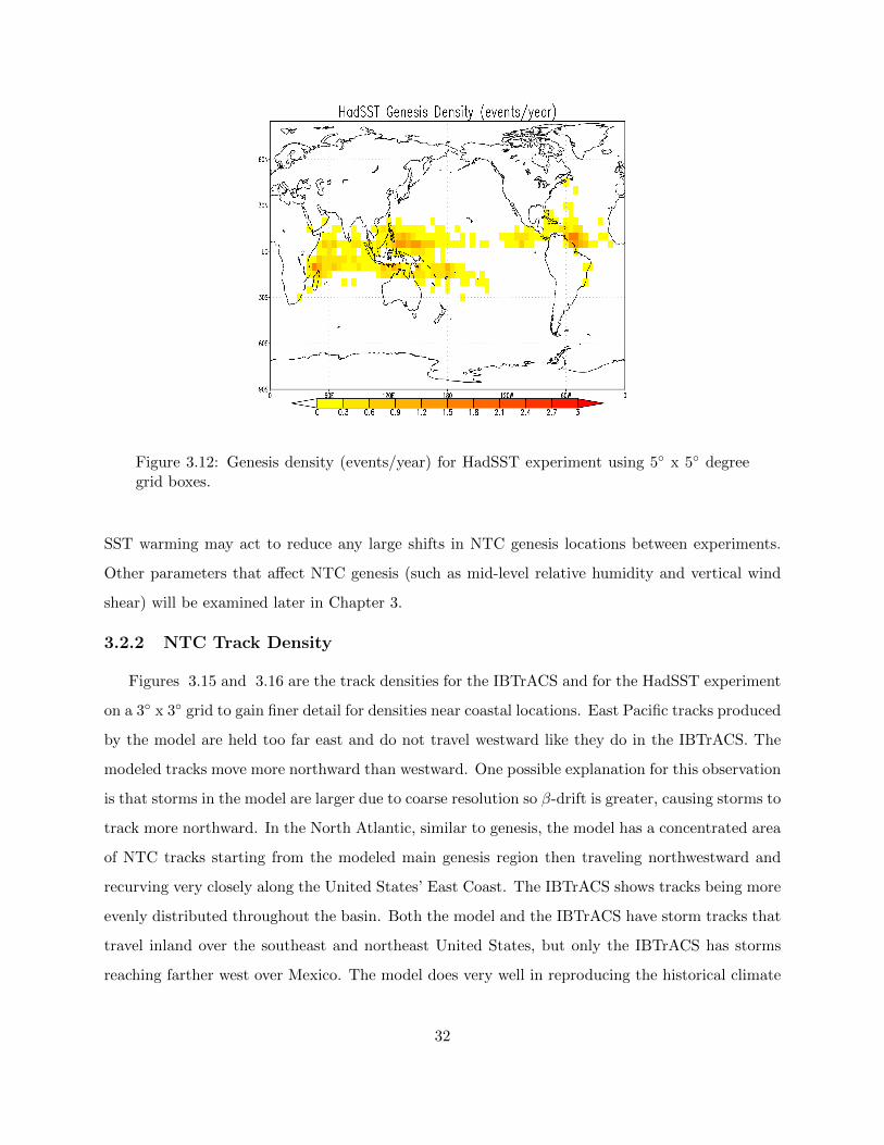
Figure 3.12: Genesis density (events/year) for HadSST experiment using 5◦ x 5◦ degreegrid boxes.

SST warming may act to reduce any large shifts in NTC genesis locations between experiments.

Other parameters that affect NTC genesis (such as mid-level relative humidity and vertical wind

shear) will be examined later in Chapter 3.

3.2.2 NTC Track Density

Figures 3.15 and 3.16 are the track densities for the IBTrACS and for the HadSST experiment

on a 3◦ x 3◦ grid to gain finer detail for densities near coastal locations. East Pacific tracks produced

by the model are held too far east and do not travel westward like they do in the IBTrACS. The

modeled tracks move more northward than westward. One possible explanation for this observation

is that storms in the model are larger due to coarse resolution so β-drift is greater, causing storms to

track more northward. In the North Atlantic, similar to genesis, the model has a concentrated area

of NTC tracks starting from the modeled main genesis region then traveling northwestward and

recurving very closely along the United States’ East Coast. The IBTrACS shows tracks being more

evenly distributed throughout the basin. Both the model and the IBTrACS have storm tracks that

travel inland over the southeast and northeast United States, but only the IBTrACS has storms

reaching farther west over Mexico. The model does very well in reproducing the historical climate

32

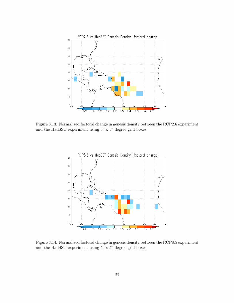
Figure 3.13: Normalized factoral change in genesis density between the RCP2.6 experimentand the HadSST experiment using 5◦ x 5◦ degree grid boxes.

Figure 3.14: Normalized factoral change in genesis density between the RCP8.5 experimentand the HadSST experiment using 5◦ x 5◦ degree grid boxes.

33

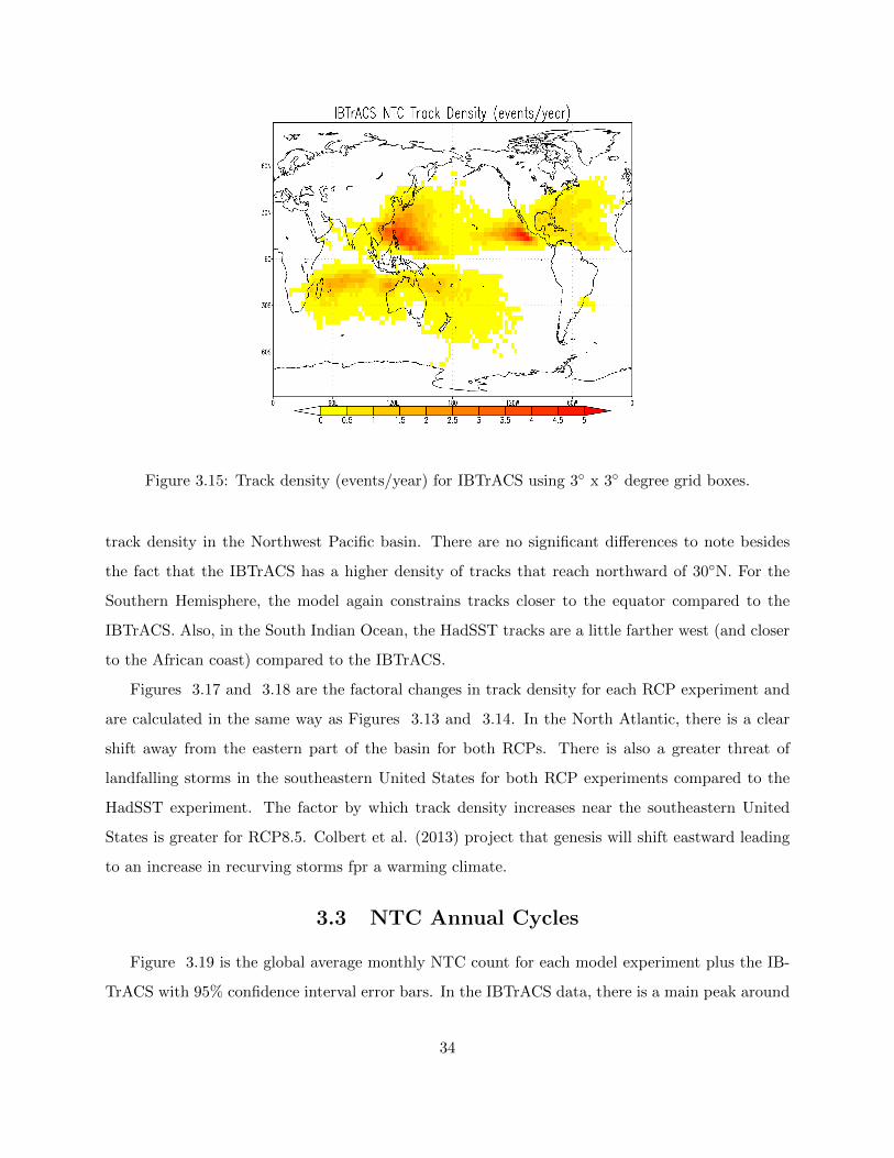
Figure 3.15: Track density (events/year) for IBTrACS using 3◦ x 3◦ degree grid boxes.

track density in the Northwest Pacific basin. There are no significant differences to note besides

the fact that the IBTrACS has a higher density of tracks that reach northward of 30◦N. For the

Southern Hemisphere, the model again constrains tracks closer to the equator compared to the

IBTrACS. Also, in the South Indian Ocean, the HadSST tracks are a little farther west (and closer

to the African coast) compared to the IBTrACS.

Figures 3.17 and 3.18 are the factoral changes in track density for each RCP experiment and

are calculated in the same way as Figures 3.13 and 3.14. In the North Atlantic, there is a clear

shift away from the eastern part of the basin for both RCPs. There is also a greater threat of

landfalling storms in the southeastern United States for both RCP experiments compared to the

HadSST experiment. The factor by which track density increases near the southeastern United

States is greater for RCP8.5. Colbert et al. (2013) project that genesis will shift eastward leading

to an increase in recurving storms fpr a warming climate.

3.3 NTC Annual Cycles

Figure 3.19 is the global average monthly NTC count for each model experiment plus the IB-

TrACS with 95% confidence interval error bars. In the IBTrACS data, there is a main peak around

34

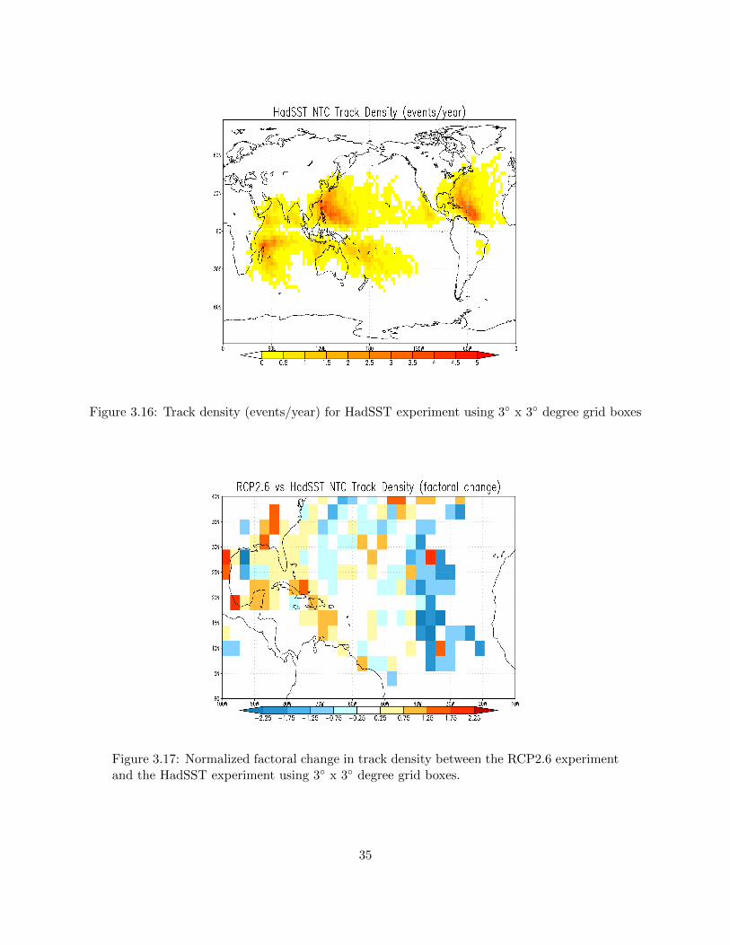
Figure 3.16: Track density (events/year) for HadSST experiment using 3◦ x 3◦ degree grid boxes

Figure 3.17: Normalized factoral change in track density between the RCP2.6 experimentand the HadSST experiment using 3◦ x 3◦ degree grid boxes.

35

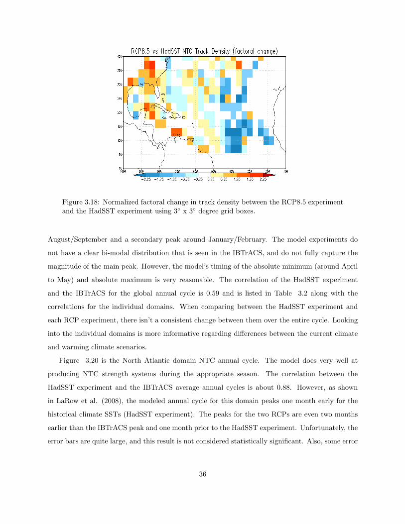
Figure 3.18: Normalized factoral change in track density between the RCP8.5 experimentand the HadSST experiment using 3◦ x 3◦ degree grid boxes.

August/September and a secondary peak around January/February. The model experiments do

not have a clear bi-modal distribution that is seen in the IBTrACS, and do not fully capture the

magnitude of the main peak. However, the model’s timing of the absolute minimum (around April

to May) and absolute maximum is very reasonable. The correlation of the HadSST experiment

and the IBTrACS for the global annual cycle is 0.59 and is listed in Table 3.2 along with the

correlations for the individual domains. When comparing between the HadSST experiment and

each RCP experiment, there isn’t a consistent change between them over the entire cycle. Looking

into the individual domains is more informative regarding differences between the current climate

and warming climate scenarios.

Figure 3.20 is the North Atlantic domain NTC annual cycle. The model does very well at

producing NTC strength systems during the appropriate season. The correlation between the

HadSST experiment and the IBTrACS average annual cycles is about 0.88. However, as shown

in LaRow et al. (2008), the modeled annual cycle for this domain peaks one month early for the

historical climate SSTs (HadSST experiment). The peaks for the two RCPs are even two months

earlier than the IBTrACS peak and one month prior to the HadSST experiment. Unfortunately, the

error bars are quite large, and this result is not considered statistically significant. Also, some error

36

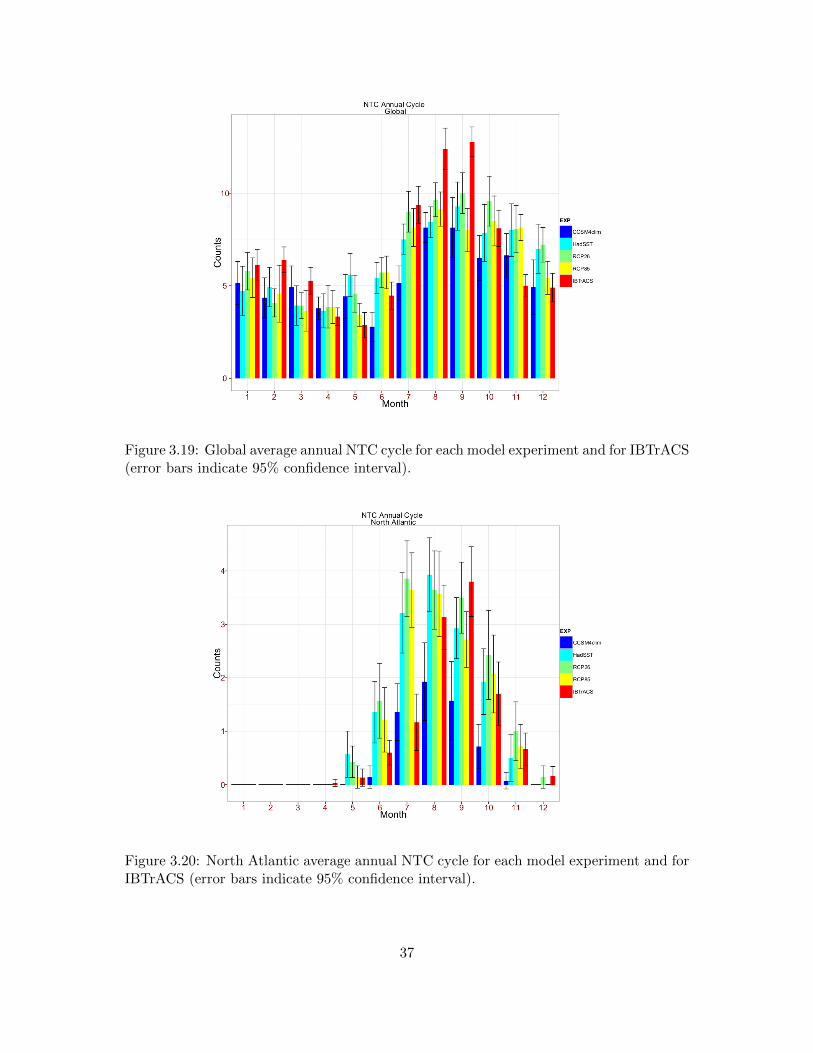
Figure 3.19: Global average annual NTC cycle for each model experiment and for IBTrACS(error bars indicate 95% confidence interval).

Figure 3.20: North Atlantic average annual NTC cycle for each model experiment and forIBTrACS (error bars indicate 95% confidence interval).

37

bars during months of less activity extend below zero which is not physical when considering NTC

frequency. Perhaps a better method for developing error bars for data in a Poisson distribution

could be used in the future.

Annual cycle plots for the remaining basins are not shown but are discussed here. The model

underestimates the number of NTCs in the Northeast Pacific domain and has a majority of the

storms later in the season compared to the IBTrACS. The correlation between the HadSST exper-

iment and the IBTrACS for the Northeast Pacific domain is 0.62. In the North Indian domain,

the IBTrACS is incomplete and all ’UNNAMED,’ ’NOT NAMED,’ ’NAMELESS,’ and ’MISSING’

storms are removed. This accounts for a non-trivial percentage of observed storms, so it is diffucult

to make a good comparison between the observations and the model experiments. In the Northwest

Pacific domain, the HadSST experiment has a correlation of 0.90 with the IBTrACS. And in the

Southern Hemisphere, the correlation between the HadSST experiment and the IBTrACS is 0.88.

Table 3.2: Rank-based correlations using Spearman’s ρ statistic for the mean annual cyclesof the HadSST experiment and IBTrACS.

Domain ρ

EPac 0.62NAtl 0.88NIn 0.83

SHem 0.88WPac 0.90Globe 0.59

3.4 Climatological Changes of Other Parameters Affecting NTCActivity

The changes in NTC activity (counts, durations, wind speeds, precipitation, and genesis and

track location) that the model projects for each RCP experiment have been calculated. The next

step is to take a look at the changes of different climatological parameters to understand why given

changes in NTC activity have occurred in the model. Some climatological parameters that are

known to strongly affect NTC activity are static stability, mid-level relative humidity, vertical wind

shear of the horizontal winds, steering flow, and tropics-relative SSTs.

38

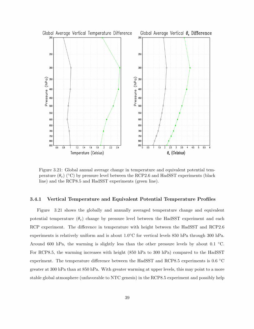
Figure 3.21: Global annual average change in temperature and equivalent potential tem-perature (θe) (◦C) by pressure level between the RCP2.6 and HadSST experiments (blackline) and the RCP8.5 and HadSST experiments (green line).

3.4.1 Vertical Temperature and Equivalent Potential Temperature Profiles

Figure 3.21 shows the globally and annually averaged temperature change and equivalent

potential temperature (θe) change by pressure level between the HadSST experiment and each

RCP experiment. The difference in temperature with height between the HadSST and RCP2.6

experiments is relatively uniform and is about 1.0◦C for vertical levels 850 hPa through 300 hPa.

Around 600 hPa, the warming is slightly less than the other pressure levels by about 0.1 ◦C.

For RCP8.5, the warming increases with height (850 hPa to 300 hPa) compared to the HadSST

experiment. The temperature difference between the HadSST and RCP8.5 experiments is 0.6 ◦C

greater at 300 hPa than at 850 hPa. With greater warming at upper levels, this may point to a more

stable global atmosphere (unfavorable to NTC genesis) in the RCP8.5 experiment and possibly help

39

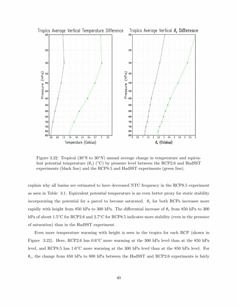
Figure 3.22: Tropical (30◦S to 30◦N) annual average change in temperature and equiva-lent potential temperature (θe) (◦C) by pressure level between the RCP2.6 and HadSSTexperiments (black line) and the RCP8.5 and HadSST experiments (green line).

explain why all basins are estimated to have decreased NTC frequency in the RCP8.5 experiment

as seen in Table 3.1. Equivalent potential temperature is an even better proxy for static stability

incorporating the potential for a parcel to become saturated. θe for both RCPs increases more

rapidly with height from 850 hPa to 300 hPa. The differential increase of θe from 850 hPa to 300

hPa of about 1.5◦C for RCP2.6 and 2.7◦C for RCP8.5 indicates more stability (even in the presence

of saturation) than in the HadSST experiment.

Even more temperature warming with height is seen in the tropics for each RCP (shown in

Figure 3.22). Here, RCP2.6 has 0.6◦C more warming at the 300 hPa level than at the 850 hPa

level, and RCP8.5 has 1.6◦C more warming at the 300 hPa level than at the 850 hPa level. For

θe, the change from 850 hPa to 800 hPa between the HadSST and RCP2.6 experiments is fairly

40

uniform at about 1.2◦C and increasing to 3.0◦C at 200 hPa. The difference between the HadSST

and RCP8.5 experiments increases steadily with height from about 2◦C at 850 hPa to about 6.0◦C

at 200 hPa. The tropical atmosphere becomes more stable for RCP8.5 than for RCP2.6. This may

be one reason that the changes in NTC frequency are mixed in sign for all domains for the RCP2.6

experiment but are all negative for the RCP8.5 experiment.

Changes in 700 hPa relative humidity are also compared between model experiments. Patterns

of moistening and drying in the mid-levels for the North Atlantaic domain are similar for both

RCP experiments compared to the HadSST experiment with magnitudes being greatest for RCP8.5

(although statistical significance was not determined). Drying occurs in the MDR while moistening

occurs north and south of the MDR. These possible changes might be a result of an overall shift in

tropical circulations and/or the location of the Inter-Tropical Convergence Zone (ITCZ). The area

of drying could have a significant effect on NTC genesis, duration, and strength.

3.4.2 Vertical Wind Shear

The percent differences in 850 hPa to 200 hPa vertical wind sheer between each RCP experiment

and the HadSST experiment is seen in Figure 3.23 (colored contours). Hatching indicates areas

where the differences are statistically significant to the 95% level. There is generally a statistically

significant increase in the magnitude of wind shear for the main development region of the North

Atlantic domian for both RCP experiments compared to the HadSST experiment. Interestingly, the

greatest increases in wind shear occur in the western part of the domain for both RCP experiments.

This is a potential reason for the model to produce genesis more frequently in the eastern part of

the domain (as seen is Figures 3.13 and 3.14). This could also contribute to the track shifts

toward the eastern part of the domain as seen in Figures 3.17 and 3.18. Also, a smaller area of

statistically significantly less wind shear exists over Florida and part of the Caribbean region for

RCP2.6. This might even be a result of the increased NTC activity near the southeastern United

States that is produced in the model for that experiment.

3.4.3 Tropics-relative SSTs

As mentioned in Chapter 2, an increase in tropics-relative SST is more important than a uniform

increase of SSTs over the entire tropics when considering NTC activity in the North Atlantic domain

(Vecchi and Soden 2007; Swanson 2008; Villarini and Vecchi 2012; Sun et al. 2013). Using the

41

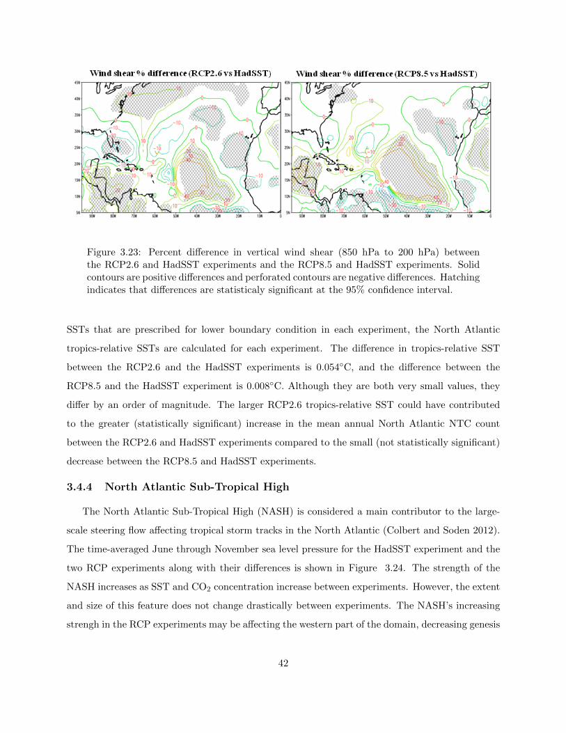
Figure 3.23: Percent difference in vertical wind shear (850 hPa to 200 hPa) betweenthe RCP2.6 and HadSST experiments and the RCP8.5 and HadSST experiments. Solidcontours are positive differences and perforated contours are negative differences. Hatchingindicates that differences are statisticaly significant at the 95% confidence interval.

SSTs that are prescribed for lower boundary condition in each experiment, the North Atlantic

tropics-relative SSTs are calculated for each experiment. The difference in tropics-relative SST

between the RCP2.6 and the HadSST experiments is 0.054◦C, and the difference between the

RCP8.5 and the HadSST experiment is 0.008◦C. Although they are both very small values, they

differ by an order of magnitude. The larger RCP2.6 tropics-relative SST could have contributed

to the greater (statistically significant) increase in the mean annual North Atlantic NTC count

between the RCP2.6 and HadSST experiments compared to the small (not statistically significant)

decrease between the RCP8.5 and HadSST experiments.

3.4.4 North Atlantic Sub-Tropical High

The North Atlantic Sub-Tropical High (NASH) is considered a main contributor to the large-

scale steering flow affecting tropical storm tracks in the North Atlantic (Colbert and Soden 2012).

The time-averaged June through November sea level pressure for the HadSST experiment and the

two RCP experiments along with their differences is shown in Figure 3.24. The strength of the

NASH increases as SST and CO2 concentration increase between experiments. However, the extent

and size of this feature does not change drastically between experiments. The NASH’s increasing

strengh in the RCP experiments may be affecting the western part of the domain, decreasing genesis

42

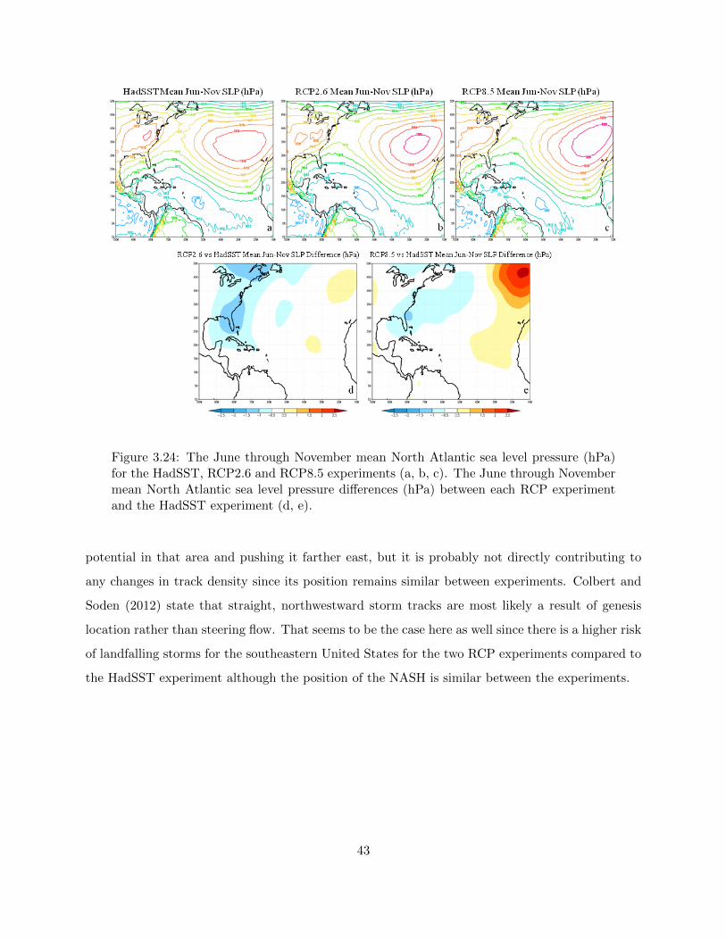
Figure 3.24: The June through November mean North Atlantic sea level pressure (hPa)for the HadSST, RCP2.6 and RCP8.5 experiments (a, b, c). The June through Novembermean North Atlantic sea level pressure differences (hPa) between each RCP experimentand the HadSST experiment (d, e).

potential in that area and pushing it farther east, but it is probably not directly contributing to

any changes in track density since its position remains similar between experiments. Colbert and

Soden (2012) state that straight, northwestward storm tracks are most likely a result of genesis

location rather than steering flow. That seems to be the case here as well since there is a higher risk

of landfalling storms for the southeastern United States for the two RCP experiments compared to

the HadSST experiment although the position of the NASH is similar between the experiments.

43

CHAPTER 4

DISCUSSION AND CONCLUSIONS

CO2 concentrations have risen throughout the 20th century and are expected to continue increasing

throughout the 21st century. This anthropogenic forcing could lead to climatological changes in

parameters that affect TC activity such as atmospheric temperatures, SSTs, moisture, wind shear,

static stability, and tropical circulations. Additionally, these changes won’t likely occur uniformly

across all TC domains. This further complicates any efforts to project future TC climatology. Also,

the rates at which these parameters (and TC activity) will change will depend on factors like policy

and technology. At this time, the best that can be done is to use multiple future climate scenarios

to estimate the potential changes in NTC activity for each scenario through climate modeling.

4.1 Experiment Summary

Models that do well at reproducing historical NTC climatology are the best candidates to make

future NTC climatology estimates. The FSU/COAPS model has done very well at reproducing

interannual variability of hurricane counts for the North Atlantic basin over the period 1982–2009

with a mean correlation of 0.74. In this study, the FSU/COAPS model is used to estimate the

2006–2100 NTC activity climatology for two future climate scenarios (RCP2.6 and RCP8.5). This

is done by taking the mean CO2 concentrations over that period and the monthly mean CCSM4

bias-corrected future projected SSTs over that period and using them to force the FSU/COAPS

model. Another model experiment (the control experiment) is done using monthly mean historically

observed SSTs and a historical CO2 concentration. A NTC detection/tracking algorithm is applied

to these three model experiments to obtain statistics for NTC counts, intensities, locations, and

durations. These statistics are compared between the model experiments to determine if any

future changes in NTC activity are projected by the model. Furthermore, other variables from

each experiment such as static stability, relative humidity, vertical wind shear, tropics-relative

SSTs (from the model’s lower boundary conditions), and sea level pressure patterns are examined

44

in an effort to understand the physical processes that might be leading to any projected changes

in TC activity.

4.2 Global Discussion

The model projects a small increase in global NTC frequency for RCP2.6 and a small decrease

in NTC frequency for RCP8.5 compared to the HadSST experiment. Neither change is statistically

significant (using a 95% level). Most similar published modeling studies have projected either no

change or a decrease in global NTC frequency in a warming climate (Knutson et al. 2010). Also

in this study, the global distribution of storms seems to shift from the largest percentage in the

Southern Hemisphere (compared to individual Northern Hemisphere domains) for the HadSST

experiment to the Northwest Pacific domain for the warmest SST experiment (RCP8.5). Other

modeling studies also found a shift in global NTC distribution from the Southern Hemisphere to

the Northern Hemisphere (Knutson et al. 2010).

4.3 North Atlantic Discussion

In the North Atlantic domain, the model projects a statistically significant increase of 14.9% for

climatological NTC frequency for the RCP2.6 scenario. After investigating multiple parameters that

may influence NTC frequency, a higher tropics-relative SST for the RCP2.6 experiment compared to

the HadSST experiment is suspected to be the most influential cause for the difference in frequency.

The RCP8.5 scenario has a similar tropics-relative SST to that of the HadSST experiment which

helps explain why the projected change in NTC frequency between those two experiments was

not statistically significant. Although previously published studies have mixed projections in NTC

frequency for the North Atlantic basin, this study agrees with the suggestion that tropics-relative

SST is more influential on NTC frequency than a uniform change in SST. Also, a statistically

significant increase in the frequency of the highest wind speeds that can be resolved by the model is

found in this study for the RCP8.5 experiment (greatest warming scenario). This could be a result

of climatological changes like an increase in overall SST (providing more energy to storms). Storms

are also found to have greater precipitation with increasing SST. All three experiements (HadSST,

RCP2.6, and RCP8.5) had statistically significantly different amounts of precipitation per day,

increasing with increasing SST. Therefore, tropics-relative SST changes seem to be most important

45

for NTC frequency while overall SST changes seem to be most important for NTC intensity (wind

speed and precipitation).

Genesis and storm tracks in the North Atlantic basin are more concentrated in the western part

of the basin for both the RCP2.6 and RCP8.5 experiments. Two factors that may be influencing

therse changes are statistically significantly increasing vertical wind shear in the eastern part of

the domain and a strengthening sub-tropical high pattern for the RCP2.6 and RCP8.5 experiments

(compared to the HadSST experiment). This could also be a result of a preferred region of genesis

within the model.

4.4 Continued Research

The results from this study can be added to the existing studies on climate modeling projec-

tions for various future climate scenarios. This study supports the theory that the North Atlantic

domain’s tropics-relative SSTs have a greater effect on NTC frequency than uniformly warming

tropical SSTs. However, since statistically significant results were found for only the RCP2.6

experiment in the North Atlantic (and neither RCP experiment for the Globe), ideally more in-

tegrations for each experiment should be done to develop a larger ensemble size in an effort to

develop more significant results. Then, the FSU/COAPS model’s future climate projections can

be better compared with other similar studies. Similarly, a larger ensemble size might also help

reveal any differences in NTC intensity between the HadSST and RCP2.6 experiments which were

not found to be statistically significantly different in this study. It might also be beneficial to force

the model with future climate scenario SSTs and CO2 concentrations that are representative of a

shorter period at the end of the 21st century (possibly 2090–2100) rather than a climatology of

the entire 2006–2100 period. Such an experiment might be more useful since NTC activity at the

beginning and end of the 21st century may be very different. That difference is not represented by

taking a climatology over nearly the entire century.

46

REFERENCES

Bender, M. A., T. R. Knutson, R. E. Tuleya, J. J. Sirutis, G. A. Vecchi, S. T. Garner, and I. M.Held, 2010: Modeled impact of anthropogenic warming on the frequency of intense Atlantichurricanes. Science, 327, 454–458.

Bengtsson, L., M. Botzet, and M. Esch, 1996: Will greenhouse gas-induced warming over the next50 years lead to higher frequency and greater intensity of hurricanes?. Tellus, 48A, 57–73.

Bengtsson, L., K. I. Hodges, M. Esch, N. Keenlyside, L. Kornblueh, J.-J. Luo, and T. Yamagata,2007: How may tropical cyclones change in a warmer climate?. Tellus, 59A, 539–561.

Chang, E. K. M., and Y. Guo, 2007: Is the number of North Atlantic tropical cyclones significantlyunderestimated prior to the availability of satellite observations?. Geophys. Res. Lett., 34,L14801, doi:10.1029/2007GL030169.

Charney, J. G., and J. Shukla, 1981: Predictability of monsoons. Monsoon dynamics, J. Lighthilland R. P. Pearce, Eds., Cambridge University Press, 99–109.

Cocke, S. E., and T. E. LaRow, 2000: Seasonal predictions using a regional spectral model embed-ded within a coupled ocean-atmosphere model. Mon. Wea. Rev., 128, 689–708.

Colbert, A. J., and B. J. Soden, 2012: Climatological variations in North Atlantic tropical cyclonetracks. J. Climate, 25, 657–673.

Colbert, A. J, B. J. Soden, G. A Vecchi, and B. P. Kirtman, 2013: The impact of anthropogenicclimate change on North Atlantic tropical cyclone tracks. J. Climate, 26, 4088–4095.

Emanuel, K. R., 2007: Environmental factors affecting tropical cyclone power dissipation. J.Climate, 20, 5497–5509.

Emanuel, K., R. Sundararajan, and J. Williams, 2008: Hurricanes and global warming: resultsfrom downscaling IPCC AR4 simulations. Bull. Amer. Meteor. Soc., 89, 347–367.

Emanuel, K. A., 2013: Downscaling CMIP5 models shows increased tropical cyclone activity overthe 21st century. Proc. Natl. Acad. Sci. USA, 110, 12,219–12,224. doi:10.1073/pnas.1301293110.

Gent, P. R., G. Danabasoglu, L. J. Donner, M. M. Holland, E. C. Hunke, S. R. Jayne, D. M.Lawrence, R. B. Neale, P. J. Rasch, M. Vertenstein, P. H. Worley, Z.-L. Yang, and M. Zhang,2011: The Community Climate System Model version 4. J. Climate, 24, 4973–4991.

Goldenberg, S. B., C. W. Landsea, A. M. Mestas-Nunez, and W. M. Gray, 2001: The recent increasein Atlantic hurricane activity: Causes and implications. Science, 293, 474–479.

47

Gray, W. M, 1975: Tropical cyclone genesis. Dept. of Atmos. Sci. Paper No. 323, Colorado StateUniversity, Ft. Collins, CO 80523, 121 pp.

Held, I. M., and M. Zhao, 2011: The response of tropical cyclone statistics to an increase in CO2

with fixed sea surface temperatures. J. Climate, 24, 5353–5364.

Henderson-Sellers, A., H. Zhang, G. Berz, K. Emanuel, W. Gray, C. Landsea, G. Holland, J.Lighthill, S.-L. Shieh, P. Webster, and K. McGuffie, 1998: Tropical cyclones and globalclimate change: A post-IPCC assessment. Bull. Amer. Meteor. Soc., 79, 19–38.

Holland, G. J., and P. J. Webster, 2007: Heightened tropical cyclone activity in the North Atlantic:Natural variability or climate trend?. Philos. Trans. Roy. Soc. Math. Phys. Eng. Sci.,365A, 2695–2716.

Knapp, K. R., M. C. Kruk, D. H. Levinson, H. J. Diamond, and C. J. Neumann, 2010: The Inter-national Best Track Archive for Climate Stewardship (IBTrACS): Unifying tropical cyclonebest track data. Bull. Amer. Meteor. Soc., 91, 363–376.

Knutson, T. R., J. J. Sirutis, S. T. Garner, I. M. Held, and R. E. Tuleya, 2007: Simulation ofthe recent multidecadal increase of Atlantic hurricane activity using an 18-km-grid regionalmodel. Bull. Amer. Meteor. Soc., 88, 1549–1565.

Knutson, T. R., J. J. Sirutis, S. T. Garner, G. A. Vecchi, and I. M. Held, 2008: Simulated reductionin Atlantic hurricane frequency under twenty-first-century warming conditions. Nat. Geosci.,1, 359–364.

Knutson, T. R., J. L. McBride, J. Chan, K. Emanuel, G. Holland, C. Landsea, I. Held, J. P. Kossin,A. K. Srivastava, and M. Sugi, 2010: Tropical cyclones and climate change. Nat. Geosci., 3,157–163, doi:10.1038/NGEO779.

Landsea, C. W., 2007: Counting Atlantic tropical cyclones back in time. Eos, Trans. Amer.Geophys. Union, 88, 197–203.

LaRow, T. E., Y.-K. Lim, D. W. Shin, E. P. Chassignet, and S. Cocke, 2008: Atlantic basin seasonalhurricane simulations. J. Climate, 21, 3191–3206.

LaRow, T. E., L. Stefanova, D.-W. Shin, and S. Cocke, 2010: Seasonal Atlantic tropical cyclonehindcasting/forecasting using two sea surface temperature datasets. Geophys. Res. Lett., 37,L02804, doi:10.1029/2009GL041459.

LaRow, T. E., 2013: The impact of SST bias correction on North Atlantic hurricane retrospectiveforecasts. Mon. Wea. Rev., 141, 490–498.

Lorenz, E. N., 1963: Deterministic Nonperiodic Flow. J. Atmos. Sci., 20, 130–141.

48

Liu, H., C. Wang, S.-K. Lee, and D. Enfield, 2013: Atlantic warm pool variability in the CMIP5simulations. J. Climate, 26, 5315–5336.

Mann, M. E., and K. A. Emanuel, 2006: Atlantic hurricane trends linked to climate change. Eos,Trans. Amer. Geophys. Union, 87, 233–244.

Meinshausen, M., S. J. Smith, K. Calvin, J. S. Daniel, M. L. T. Kainuma, J.-F. Lamarque, K.Matsumoto, S. A. Montzka, S. C. B. Raper, K. Riahi, A. Thomson, G. J. M. Velders, and D.P. P. van Vuuren, 2011: The RCP greenhouse gas concentraions and their extensions from1765 to 2300. Clim. Change, 109, 213–241.

Rayner, N. A., D. E. Parker, E. B. Horton, C. K. Folland, L. V. Alexander, D. P. Rowell, E.C. Kent, and A. Kaplan, 2003: Global analyses of sea surface temperature, sea ice, andnight marine air temperature, since the late nineteenth century. J. Geophys. Res., 108,doi:10.1029/2002JD002670.

Santer, B. D., and Coauthors, 2006: Forced and unforced ocean temperature changes in Atlanticand Pacific tropical cyclogenesis regions. Proc. Natl. Acad. Sci. USA, 103, 13,905–13,910.

Schenkel, B. A., and R. E. Hart, 2011: Examination of tropical cyclone position, intensity, andintensity life cycle within atmospheric reanalysis datasets. J. Climate, 25, 3453–3475.

Shukla, J., 1998: Predictability in the midst of chaos: A scientific basis for climate forecasting.Science, 282, 728–731.

Stefanova, L. and T. LaRow, 2011: Low-frequency SST variabilityin CMIP-5 historical integra-tions. 36th NOAA Climate Diagnostics and Prediction Workshop, Special Issue Science andTechnology Infusion Climate Bulletin, NOAA’s National Weather Service, 116-118.

Strazzo, S., J. B. Elsner, T. LaRow, D. J. Halperin, and M. Zhao, 2013: Observed versus GCM-generated local tropical cyclone frequency: Comparisons using a spatial lattice. J. Climate,26, 8257–8268.

Sugi, M., A. Noda, N. Sato, 2002: Influence of the global warming on tropical cyclone climatology:An experiment with the JMA global model. J. Meteor. Soc. Japan, 80, 249–272.

Sun, Y., Z. Zhong, Y. Ha, Y. Wang, and X. D. Wang, 2013: The dynamic and thermodynamicperspectives of relative and absolute sea surface temperature on tropical cylcone intensity.Acta Meteorol. Sin., 27, 40–49.

Swanson, K., 2008: Nonlocality of Atlantic tropical cyclone intensities. Geochem. Geophys.Geosys., 9, Q04V01. doi:10.1029/2007GC001844.

Tang, B. H., and J. D. Neelin, 2004: ENSO influence on Atlantic hurricanes via troposphericwarming. Geophys. Res. Lett., 31, L24204, doi:10.1029/2004GL021072.

49

Taylor, K. E., R. J. Stouffer, and G. A. Meehl, 2009: A summary of the CMIP5 experiment design.33 pp., cmip-pcmdi.llnl.gov.

Taylor, K. E., R. J. Stouffer, and G. A. Meehl, 2012: An overview of CMIP5 and the experimentdesign. Bull. Amer. Meteor. Soc., 93, 485–498.

Vecchi, G. A., and B. J. Soden, 2007: Effect of remote sea surface temperature change on tropicalcylcone potential intensity. Nature, 450, 1066–1070.

Vecchi, G. A., and T. R. Knutson, 2008: On estimates of historical North Atlantic tropical cycloneactivity. J. Climate, 21, 3580–3600.

Villarini, G., and G. A. Vecchi, 2012: Twenty-first-century projections of North Atlantic tropicalstorms from CMIP5 models. Nat. Climate Change, 2, 604–607.

Villarini, G., and G. A. Vecchi, 2013: Projected increases in North Atlantic tropical cyclone inten-sity from CMIP5 models. J. Climate, textbf26, 3231–3240.

Walsh, K. J. E., M. Fiorino, C. W. Landsea, and K. L. McInnes, 2007: Objectively determinedresolution-dependent threshold criteria for the detection of tropical cyclones in climate modelsand reanalyses. J. Climate, 20, 2307–2314.

Webster, P. J., G. J. Holland, J. A. Curry, and H.-R. Chang, 2005: Changes in tropical cyclonenumber, duration, and intensity in a warming environment. Science, 309, 1844–1846.

Zhao, M., I. M. Held, S.-J. Lin, and G. A. Vecchi, 2009: Simulations of global hurricane climatology,interannual variability, and response to global warming using a 50-km resolution GCM. J.Climate, 22, 6653–6678.

Zhao, M., and I. M. Held, 2012: TC-permitting GCM simulations of hurricane frequency responseto sea surface temperature anomalies projected for the late-twenty-first century. J. Climate,textbf25, 2995–3009.

50

BIOGRAPHICAL SKETCH

I grew up living with my mother (Kandra) in Hartville, Ohio. I have always enjoyed learning math

and science which led to my interest in Meteorology. I attended North Carolina State University

where I received my B. S. degree in Meteorology and graduated as a valedictorian with a 4.0 GPA.

I did not have a chance during my undergraduate career to learn about tropical meteorology, so

I wanted to attend a graduate school where I could learn more about that topic. That led me to

Florida State University. I have worked with Dr. LaRow at the Center for Ocean-Atmospheric

Prediction Studies (COAPS) on research that concentrates on how future climate change might

affect tropical cyclone activity. My plan after graduating is to find a research-oriented Meteorology

job.

51