ESTIMATING THE MARKET VALUE OF FRANKING CREDITS: … · weighted average cost of capital in Australian regulatory decisions. There is, however, a lack of consensus on an appropriate

ESTIMATING THE MARKET VALUE OF FRANKING CREDITS:

EMPIRICAL EVIDENCE FROM AUSTRALIA

Duc Vo

Beauden Gellard

Stefan Mero

Economic Regulation Authority

469 Wellington Street, Perth, WA 6000, Australia

Phone: (08) 6557 7900

Fax: (08) 6488 1016

April 2013

* We are greatly indebted to Greg Watkinson, Rajat Sarawat and Bruce Layman for the support and constructive

comments they have provided during the writing of this paper. Special thanks to Kieu Pham and Bill Scalan for their proofreading. The views expressed herein in this paper are those of the authors and do not necessarily represent those of the Secretariat or the Economic Regulation Authority. All remaining errors are ours.

ESTIMATING THE MARKET VALUE OF FRANKING CREDITS:

EMPIRICAL EVIDENCE FROM AUSTRALIA

Abstract

The market value of franking credits, known as theta, is an important input for estimating the

weighted average cost of capital in Australian regulatory decisions. There is, however, a lack of consensus on an appropriate estimate of the market value of franking credits. This paper attempts

to estimate the market value of franking credits using a dividend drop-off methodology. A list of

2,595 unique tickers was compiled by observing stocks listed on the ASX during the period 1 July

2001 to 1 July 2012. Dividend distribution events from 1 July 2001 to 1 July 2012 were obtained and a dividend sample was constructed using filters identified in literature on the topic. Regression

techniques and parametric forms of the dividend drop–off equation were also sourced from relevant

literature. Initial estimates of the value of theta were calculated, and then a sensitivity analysis was performed to ascertain the robustness of the estimates. It was found that due to the high

multicolinearity between the net dividend and the franking credit, precise estimates of theta could

not be readily obtained. . Because of this, it may be more appropriate to use a range for the value of theta rather than a derived point estimate. The appropriate range suggested by this study is

between 0.35 and 0.55.

JEL Classification Numbers: G01; G11; G18

Keywords: Franking credits; Dividend events; Dividend Drop-off methodology; regulation;

Australia.

April 2013

I Introduction

Personal taxes impact the required rate of return an investor requires on both equity and debt. It is the

post-tax (as opposed to pre-tax) rate of return that investors consider when evaluating investment

opportunities. As a consequence, it is vital to consider the implication of personal taxation on the WACC estimate. Specifically, given that Australia has an imputation tax system; its impact on the

required return to equity must be considered.

The purpose of the imputation tax system is to avoid corporate profits being taxed twice. Previously, company profits were taxed at the corporate level, and taxed again in the form of dividends paid out to

shareholders as personal income tax. Under the Australian imputation tax system, a franking credit is

distributed to individuals with dividends to offset personal taxation liability. The franking credit

represents the amount of personal taxation already paid at the corporate level. Imputation credits in Australia have a face value of one dollar per credit which can be claimed as a rebate to offset personal

tax liabilities. Since the 1st July 2000, a refund on any excess credits over personal tax liabilities can

be claimed. It is important to note that international investors cannot utilise imputation tax credits. As such, imputation tax credits provide benefits to Australian investors only.

Any value generated by the presence of franking credits in the Australian tax system must be

accounted for in the required return to equity, and in turn the weighted average cost of capital.

Investors would be willing to accept a relatively lower required rate of return on an investment that has franking credits compared with an investment with similar risk and without a benefit of franking

credits. The precise value investors place on franking credits is ambiguous, given that individual

investors have differing taxation circumstances and personal franking credit valuations.

II Theoretical Background

(i) Gamma in the Weighted Average Cost of Capital

Franking credits represent a rebate which reduces personal taxation liabilities. As franking credits

alter the effective after-tax return on an equity investment; franking credits will alter the required return on equity an investor requires. An early theoretical framework presenting how franking credits

alter the after-tax cost of capital was proposed by Officer (1994). The operating income (or Earnings

before Interest and Tax, (EBIT) of a company is defined as follows:

0 G D EX X X X (1)

where 0X is the operating income, GX is the government’s share of operating income (i.e. company

taxation), DX is the debt holders’ share of operating income and EX is the equity holder’s share of

operating income.

The amount ( )O DT X X is the amount of company taxation collected from the company by the

government. However, a proportion of this amount, which is defined as γ (gamma), represents the tax

collected from the company which will be rebated against personal income tax. It is convenient to

consider gamma as the proportion of personal income tax collected at the company level. As a consequence, the effective company taxation is defined as:

( ) ( )

( )(1 )

G O D O D

O D

X T X X T X X

T X X

(2)

Therefore, in this representation, gamma is the proportion of tax collected from the company which

gives rise to franking credits. Gamma can be considered as the proportion of company tax that is used

as prepayment of personal tax liabilities (Hathaway &Officer 2004).

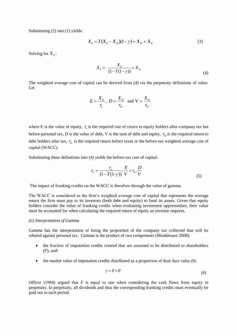
Substituting (2) into (1) yields:

0 0( )(1 )D D EX T X X X X (3)

Solving for 0X :

0

(1 (1 ))

ED

XX X

T

(4)

The weighted average cost of capital can be derived from (4) via the perpetuity definitions of value. Let

E

e

XE

r , D

D

XD

r and O

O

XV

r

where E is the value of equity, er is the required rate of return to equity holders after-company tax but

before-personal tax, D is the value of debt, V is the sum of debt and equity, Dr is the required return to

debt holders after tax, Or is the required return before taxes or the before-tax weighted average cost of

capital (WACC).

Substituting these definitions into (4) yields the before-tax cost of capital:

. .(1 (1- ))

eo d

r E Dr r

T V V

(5)

The impact of franking credits on the WACC is therefore through the value of gamma.

The WACC is considered as the firm’s weighted average cost of capital that represents the average return the firm must pay to its investors (both debt and equity) to fund its assets. Given that equity

holders consider the value of franking credits when evaluating investment opportunities, their value

must be accounted for when calculating the required return of equity an investor requires.

(ii) Interpretation of Gamma

Gamma has the interpretation of being the proportion of the company tax collected that will be

rebated against personal tax. Gamma is the product of two components (Monkhouse 2008):

the fraction of imputation credits created that are assumed to be distributed to shareholders

(F); and-

the market value of imputation credits distributed as a proportion of their face value (θ).

F (6)

Officer (1994) argued that F is equal to one when considering the cash flows from equity in

perpetuity. In perpetuity, all dividends and thus the corresponding franking credits must eventually be paid out in each period.

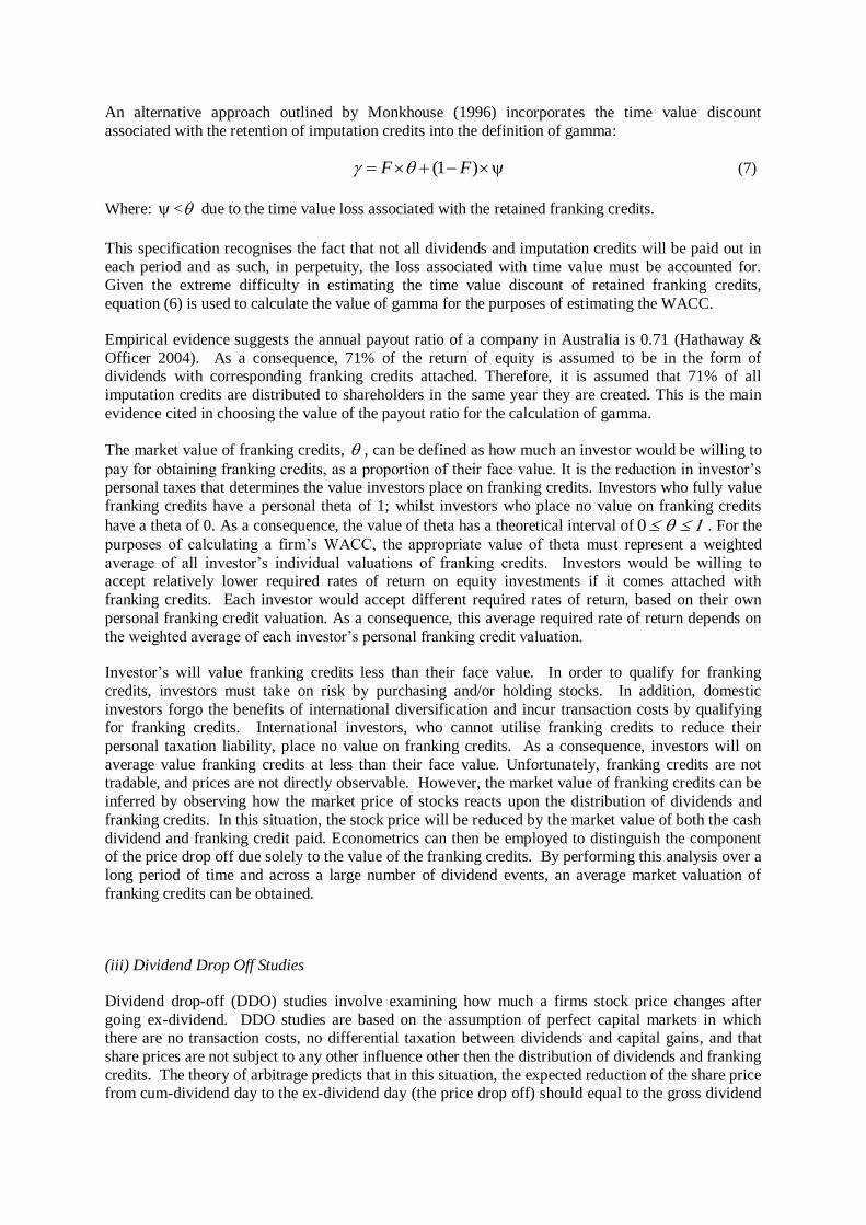
An alternative approach outlined by Monkhouse (1996) incorporates the time value discount

associated with the retention of imputation credits into the definition of gamma:

(1 )F F (7)

Where: < due to the time value loss associated with the retained franking credits.

This specification recognises the fact that not all dividends and imputation credits will be paid out in

each period and as such, in perpetuity, the loss associated with time value must be accounted for. Given the extreme difficulty in estimating the time value discount of retained franking credits,

equation (6) is used to calculate the value of gamma for the purposes of estimating the WACC.

Empirical evidence suggests the annual payout ratio of a company in Australia is 0.71 (Hathaway &

Officer 2004). As a consequence, 71% of the return of equity is assumed to be in the form of dividends with corresponding franking credits attached. Therefore, it is assumed that 71% of all

imputation credits are distributed to shareholders in the same year they are created. This is the main

evidence cited in choosing the value of the payout ratio for the calculation of gamma.

The market value of franking credits, , can be defined as how much an investor would be willing to

pay for obtaining franking credits, as a proportion of their face value. It is the reduction in investor’s personal taxes that determines the value investors place on franking credits. Investors who fully value

franking credits have a personal theta of 1; whilst investors who place no value on franking credits

have a theta of 0. As a consequence, the value of theta has a theoretical interval of 0 . For the

purposes of calculating a firm’s WACC, the appropriate value of theta must represent a weighted

average of all investor’s individual valuations of franking credits. Investors would be willing to accept relatively lower required rates of return on equity investments if it comes attached with

franking credits. Each investor would accept different required rates of return, based on their own

personal franking credit valuation. As a consequence, this average required rate of return depends on

the weighted average of each investor’s personal franking credit valuation.

Investor’s will value franking credits less than their face value. In order to qualify for franking

credits, investors must take on risk by purchasing and/or holding stocks. In addition, domestic

investors forgo the benefits of international diversification and incur transaction costs by qualifying for franking credits. International investors, who cannot utilise franking credits to reduce their

personal taxation liability, place no value on franking credits. As a consequence, investors will on

average value franking credits at less than their face value. Unfortunately, franking credits are not tradable, and prices are not directly observable. However, the market value of franking credits can be

inferred by observing how the market price of stocks reacts upon the distribution of dividends and

franking credits. In this situation, the stock price will be reduced by the market value of both the cash

dividend and franking credit paid. Econometrics can then be employed to distinguish the component of the price drop off due solely to the value of the franking credits. By performing this analysis over a

long period of time and across a large number of dividend events, an average market valuation of

franking credits can be obtained.

(iii) Dividend Drop Off Studies

Dividend drop-off (DDO) studies involve examining how much a firms stock price changes after

going ex-dividend. DDO studies are based on the assumption of perfect capital markets in which there are no transaction costs, no differential taxation between dividends and capital gains, and that

share prices are not subject to any other influence other then the distribution of dividends and franking

credits. The theory of arbitrage predicts that in this situation, the expected reduction of the share price from cum-dividend day to the ex-dividend day (the price drop off) should equal to the gross dividend

which includes the value of the cash dividend and the value of the franking credit. However, the

assumption of perfect capital markets is unlikely to hold in reality. In addition, given that investors will not fully value the combined package of the gross dividend, the expected price drop-off should be

less than that of the face value.

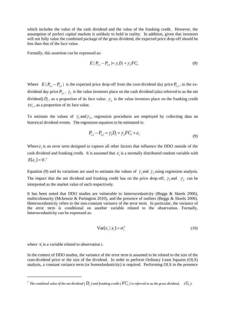
Formally, this assertion can be expressed as:

, , 1 2| |c i x i i iE P P D FC (8)

Where , ,| |c i x iE P P is the expected price drop-off from the cum-dividend day price

,c iP , to the ex-

dividend day price,x iP . 1 is the value investors place on the cash dividend (also referred to as the net

dividend) iD , as a proportion of its face value. 2 is the value investors place on the franking credit

iFC , as a proportion of its face value.

To estimate the values of 1 and 2 , regression procedures are employed by collecting data on

historical dividend events. The regression equation to be estimated is:

, , 1 2c i x i i i iP P D FC (9)

Where i is an error term designed to capture all other factors that influence the DDO outside of the

cash dividend and franking credit. It is assumed that i is a normally distributed random variable with

[ ] 0iE .1

Equation (9) and its variations are used to estimate the values of 1 and 2 using regression analysis.

The impact that the net dividend and franking credit has on the price drop-off, 1 and 2 can be

interpreted as the market value of each respectively.

It has been noted that DDO studies are vulnerable to heteroscedasticity (Beggs & Skeels 2006),

multicolinearity (Mckenzie & Partington 2010), and the presence of outliers (Beggs & Skeels 2006).

Heteroscedasticity refers to the non-constant variance of the error term. In particular, the variance of the error term is conditional on another variable related to the observation. Formally,

heteroscedasticity can be expressed as:

2Var[ | ]i i ix (10)

where ix is a variable related to observation i.

In the context of DDO studies, the variance of the error term is assumed to be related to the size of the

cum-dividend price or the size of the dividend. In order to perform Ordinary Least Squares (OLS)

analysis, a constant variance term (or homoskedasticity) is required. Performing OLS in the presence

1 The combined value of the net dividend ( iD ) and franking credit ( iFC ) is referred to as the gross dividend, ( iG ).

of heteroscedasticity will result in an estimator with a large variance, and incorrect standard error

(Hill, Griffiths and Lim 2008).

Multicolinearity is often cited as another issue in the DDO studies. Multicolinearity refers to the

situation where a linear relationship exists between the explanatory variables. Specifically, the

explanatory variables are correlated and tend to move together. Multicolinearity is a problem in that

the data set does not contain enough information in order to estimate the individual effects of the variables in the model precisely. Multicolinearity causes an increase in the standard errors of the

estimated regression coefficients, which implies less precision in the resulting estimate. The

consequences of multicolinearity arise if the purpose of regression is explanation; that is to explain the individual effect each dependent variable has on the independent variable. If the purpose of

regression is prediction, multicolinearity is not an issue as there is no need to separate out the

independent effects of the correlated variables. It is well documented that in situations where extreme multicolinearity arises, it is nearly impossible to separate the impact that the independent variables

have individually on the dependent variable (Berry & Feldman 1985). Multicolinearity can cause the

estimated model to be extremely sensitive to changes in the underlying sample, regression technique

used or the parametric form2 applied to the data (Berry & Feldman 1985).

In dividend-drop off studies, multicolinearity arises from the fact that the franking credit is calculated

from the size of the net dividend as follows:

1

ci i i

c

tFC D f

t

(11)

where ct is the corporate tax rate, if is the franking proportion3 and iD is the net dividend.

In the situation where all dividends are fully franked, 1,if i perfect multicolinearity exists and it is

impossible to estimate the value of franking credits. In practice, as some dividends are either partially

franked or have no franking, it is possible to estimate the value of franking credits. However, because most dividends are fully franked, there exists an extremely high degree of correlation between the

cash dividend and the franking credits. As a consequence, it becomes difficult to differentiate the

influence on the price drop off separately.

The presence of outliers is cited as another weakness of DDO studies (McKenzie & Partington 2010).

Outliers can have a large disproportionate influence on the regression coefficients, masking the

underlying trend of the rest of the data. Outliers are distinct from heteroscedasticity in that they are

not simply the result of a large variance, but rather indicate the inadequacy of the current model in explaining the data. Excluding outliers based on their influence on the regression coefficient can be

seen as a form of data mining, which may exclude important information from the analysis. An

alternative introduced by Truong and Partington (2006) is to utilise various forms of robust regression; regression techniques that are not heavily influenced by the presence of outliers.

2 The parametric form of a regression model refers to the particular form of the regression equation to be estimated. For

example, multiplying equation (9) by the inverse of the cum-dividend price for each event results in a new parametric form of the model.

3 The franking proportion represents the fraction of dividends that have franking credits attached to them. A franking proportion of 1 indicates that the dividends are fully franked; a 0 franking proportion indicates no franking credits are attached to dividends.

III Previous Australian Dividend Drop-Off Studies

(i) Hathaway and Officer (2004)

Hathaway and Officer (2004) explore a slightly different parametric form of the DDO equation. Theoretically, if both the cash dividend and franking credit are fully valued, this leads to a price drop-

off equal to the value of both the cash dividend and the face value of the franking credit. This

situation can be represented as:

i i i iP D F (12)

Where iP is the change in stock price from the cum-dividend day to the ex- dividend day, iD is the

net dividend, iF is the franking credit and i is an error term designed to capture all other factors that

influence the DDO outside of the cash dividend and franking credit.

The face value of the franking credit can be expressed as follows:

( )1

ci i i

c

tF D f

t

(13)

Where if is the franking proportion of the imputation tax credit, ct is the corporate tax rate for

observation i.

Substituting (13) into (12) produces:

( )1

ci i i i i

c

tP D D f

t

(14)

Dividing this equation by the cash dividend produces the following:

'1 ( )

1

i ci i

i c

P tf

D t

(15)

It is noted that this is the theoretical case where the value of the cash dividend and franking credit is fully valued. In the situation where cash dividends and franking credits are not fully valued, the

model becomes:

'.ii i

i

Pa b f

D

(16)

The interpretation of a is the drop-off proportion that is due to the cash component of the dividend,

and b is the drop-off proportion due to the franking credit.

Hathaway and Officer noted that the error term was inversely proportional to the dividend yield. To account for this form of heteroscedasticity, equation (16) was re-weighted by the dividend yields of

each dividend event to produce the following equation:

''. / . . / i

i i i

i

Pa Div P b Div f P

P

(17)

The dividend sample was constructed by compiling a list of all dividend events for stocks listed

within the ASX/S&P 500 index between August 1986 and August 2004. OLS was applied to equation (16) and (17) in order to produce an estimate of the value of franking credits over this period.

Hathaway and Officer concluded that net dividends are valued between 80 and 81 cents while

franking credits are valued between 49 and 52 cents for large capitalised companies. Hathaway and

Officer noted that they did not believe that their estimate of the value of franking credits was precise; however they noted that attributing a zero value to franking credits is incorrect. 4

(ii) Beggs and Skeels (2006)

Beggs and Skeels (2006) utilise the DDO methodology in order to estimate the value of cash-dividends and franking credits. Beggs and Skeels define the Gross Drop-Off Ratio (GDOR) as

follows:

C XP PGDOR

G

(18)

Where CP is the cum-dividend price, XP is the ex-dividend day price, G is the gross dividend. Based

on the previous literature explored by Beggs and Skeels, it is expected that the GDOR<1. This

implies that investors are valuing the combined package of the net dividend and franking credits at

less than their face value.

The DDO methodology in their study assumes that:

, , 0 1c i x i i iP P G (19)

Where 1 is the value that investors place on the gross dividend.

Separating the gross dividend of equation (19) into its components yields:

*

, , 1 2c i x i i i iP P D FC (20)

where: ,c iP is the cum-dividend price of dividend event i ,

*

,x iP is the market adjusted ex-dividend day

price of dividend event i , 1 is the cash drop-off ratio, 2 is the franking credit drop-off ratio, i

D is

the net dividend and i

FC is the face value of franking credits.

It is noted by Beggs and Skeels that DDO models suffer from heteroscedasticity. As such, OLS regression is not appropriate. Beggs and Skeels use the Feasible Generalised Least Squares (FGLS)

estimator approach by modelling the variance as follows:

2

0 1 2 3 ,ˆln i i i c i iW G P u (21)

Where i are the OLS residuals from (20), iW is the company size of dividend event i measured by

market capitalisation as a proportion of the All ordinaries Index, iG is the gross dividend of dividend

event i and ,c iP is the cum-dividend price of dividend event i .

With this model of variance, the fitted values of the variance are calculated for each individual

dividend observation:

2

0 1 2 3 ,ln i i i c iW G P (22)

The estimated standard deviation of each dividend event is then calculated using the estimated regression coefficients of (22). The inverse of this estimate is then used as weights in the original

DDO equation (20) and OLS is then applied to the following:

*

, ,

1 2

c i x i i i i

i i i i

P P D FC

(23)

The Beggs and Skeels study was based on the Commsec Share Portfolio data. They showed that the

GDOR was significantly less than 1 with the implication that net dividends and/or franking credits are

not fully valued by the average investor. Between 2001 and 2004, their estimated value was 80 cents for net dividends and 57 cents for franking credits.

(iii) Strategic Finance Group Consulting (2011)

Strategic Finance Group (SFG) conducted a DDO study using the Morningstar DatAnalysis database

(SFG 2011). Dividend events that had data missing or a market capitalisation of less than 0.03% of the

All Ordinaries Index were excluded from the analysis. Company announcements that occurred within

5 days of the ex-dividend date that were considered to be price sensitive resulted in the dividend event being removed from the sample.

SFG applied various scalings to the DDO equation in order to correct for heteroscedasticity. SFG

concluded from its survey of the DDO methodology that the heteroscedasticity was directly proportional to the cum dividend price, the size of the dividend paid and the historical volatility of

excess returns of the stock.5 To control for heteroscedasticity, SFG scaled the original DDO equation

, , 1 2c i x i i i iP P D FC , as follows:

Table 1

Parametric form of DDO equation used by SFG.

Model Parametric Form Scaling Factor

1 , ,c i x i i

i

i i

P P FC

D D

iD

2 , , ''

, , ,

c i e i i ii

c i c i c i

P P D FC

P P P

,c iP

3 , , '' ' ''1c i x i i

i

ii i i i i

P P FC

D D

ii iD

4 , , ' ' '

, , ,

c i x i i ii

c i i c i i c i i

P P D FC

P P P

,c i iP

Where ,, , 5

1

1: ( )

N

i ti t i t j

j

er erN

is the estimated standard deviation of excess returns of stock i

over N trading days, , ,

1

1:

N

i t i t

j

er erN

is the estimated mean of excess return of stock i over N

trading days, , , ,

:i t i t m t

er r r is the excess return of stock i over the market at time t and ,i t

r is the

return of stock i at time t ; ,m t

r is the return of the All Ordinaries Index at time t .

Robust regressions were applied to these dividend drops off models using the MM regression

estimator. SFG believed that model 4 showed the most consistent results across the robustness checks

they performed. As a result, model 4 was assigned the most weight. An average estimate of theta using model 4 was produced using the various robustness checks to produce an estimate for theta of

0.35.

(iv) Summary of Australian Dividend Drop Off Studies

A more extensive summary of Australian DDO studies can be found below:

Table 2

Summary of Australian Dividend Drop Off studies.

Author Year Data Techniques Theta

Brown & Clarke 1993

Statex, Melbourne and Australian Stock

Exchange publications, 1973 -

1991

OLS Regression 0.72

Walker & Partington 1999

Securities Industry

Research Centre of Asia-Pacific, 1995 to

1997

Not Specified 0.88 – 0.96

Hathaway & Officer 2004 Australian Tax Office and ASX/S&P 500,

1986 - 2004

Generalised Least Squares

0.49

Bellamy & Gray 2004 1995 -2002 Unknown 0.00

Beggs & Skeels 2006 CommSec Share

Portfolio 1986 - 2004 Generalised Least

Squares 0.57

SFG 2007

Securities Industry Research Centre of

Asia-Pacific and FinAnalysis, 1998 -

2006


0.23

Feuerherdt, Gray & Hall

2010

Securities Industry Research Centre of Asia-Pacific, 1995 -

2002


0.00

SFG 2011 DatAnalysis, 2000 -

2010 Generalised Least

Squares 0.35

The authors consider that studies carried out after 2001 are more relevant to the estimate of current

market value of franking credits. As such, other studies prior to 2001 were not considered in this

study.

Market value of franking credits do vary significantly across studies. It is noted that one author, Gray, was involved in 4 different studies as presented in Table 2 above, studies implemented in 2004; 2007;

2010; and 2011.

(IV) Analysis

(i) Considerations

The company taxation and imputation credit system has undergone many changes as outlined in

Beggs and Skeels (2006). A holding period of 45 days is necessary for total franking credit entitlements below $5,000 to qualify for franking credits. In addition, if an investor hedges the price

risk of the security using derivatives, the franking credits are unable to be used. More recently, from 1

July 2000, any excess franking credit can be rebated for cash and from 1 July 2001 the company

taxation rate has been reduced from 34 to 30 percent. As a consequence, the period considered in this analysis is from 1 July 2001 to 1 July 2012 to avoid structural changes in the company tax rate and

imputation credit system.

Various studies have noted that thinly traded stocks can have a confounding effect on dividend drop off regressions (Hathaway & Officer 2004, Beggs & Skeels 2006, SFG 2011). Prices must be a

reflection of an efficient trading mechanism which is unlikely to be the case when a stock trades

infrequently. Hathaway and Officer (2004) noted that:

‘There is no obvious reason why the cash dividend for Big Cap, Mid Cap and Small Cap stocks

should vary. That the results do is testament to the difficulty of estimation among these smaller stock events. Implicit in our experimental design is that stocks trade over the ex-date period, but many

stocks, particularly small cap stocks, are rather illiquid.’

They concluded that large capitalisation stocks to estimate the value of theta are the most reliable. In

addition, SFG(2011) and Beggs and Skells (2006) utilise a criterion of only including stocks that have a market capitalisation greater than 0.03% market capitalisation of the All Ordinaries Index. As a

consequence, the dividend sample used in this analysis has been constructed using the same 0.03%

market capitalisation filter. Another important filter is the removal of stocks that undergo a capitalisation change (for example, undergo a stock split) 5 trading days before or after a dividend

event. This ensures that the price drop off due to a capitalisation change has no impact on the

estimate of theta.

Individual special cash dividends are considered unreliable, as they are an irregular distribution of

excess cash reserves. As a consequence, dividend events that are classified as special cash only were

removed, consistent with other DDO studies (Beggs & Skeels 2006). However, it is common for

companies to distribute a special cash dividend in conjunction with a final or interim dividend. Removing special cash dividends in this scenario would imply that the price drop off is due solely to

the other dividend, creating an upward bias in the estimate of theta. Therefore, special cash dividends

that occur on the same day as a normal dividend event are aggregated in order to produce a combined dividend as described by Hathaway and Officer (2004). The remaining individual special cash

dividends were then removed from the sample.

Filters that exclude observations based on “price sensitive” announcements have not been utilised in this study. SFG (2011) screen dividend observations based on price sensitive announcements that

occur 5 days before the ex-dividend date. The price sensitive flag for announcements is available on

the ASX website. After this initial screening, SFG observe each observation and decide if the

announcement will have a material impact on the stock price. Observations that have a “price sensitive announcement” close to the cum- or ex-dividend date can be considered as unbiased noise,

equally likely to be positive or negative. As a consequence, removing these observations is

unnecessary; doing so may introduce a subjective element to the analysis that is undesirable. In principle, data points should not be removed after the final sample of dividends has been compiled.

Rather, different econometric methodologies that are not sensitive to outliers should be employed,

consistent with objective statistical analysis.

(ii) Regression Techniques

It has been noted that DDO studies are extremely sensitive to the sample of dividend events included

in the sample (McKenzie & Partington 2010). This is due to the assumptions of traditional Ordinary

Least Squares (OLS) regression analysis being violated; specifically the non-constant variance (heteroscedasticity); and non normality of errors (presence of outliers). In addition, due to the high

level of multicolinearity between the cash dividend and the franking credit, the coefficient estimates

are extremely sensitive to small changes in the model or data.

In mitigating the problems that exist with outliers, regression techniques that are less susceptible to

their presence will be applied. Least Absolute Deviation (LAD) estimators of linear models minimise

the sum of absolute values of the residuals which can be expressed formally as:

'

1β

min | |n

i i

i

y x

(24)

Where iy is the response variable of observation i; is a vector of regression coefficients to be

estimated; and ix is a vector of the covariates for observation i. In contrast to OLS, LAD regression

does not give increasing weight to larger residuals. As a consequence, it is less sensitive to outliers

then OLS regression.

The statistical literature has developed methodologies that are insensitive to small changes to model assumptions; including the presence of outliers. Robust statistics are methodologies designed to be

insensitive to deviations from the assumptions made in a statistical analysis (Huber 1996). In

particular, various forms of robust regression have been developed in order to limit the influence of outliers; and to deal with the violation of the normality assumption. Robust regression has also been

proposed as a method for dealing with heteroscedasticity (Andersen 2008). A central concept of

robust statistics is the breakdown point of an estimator; the smallest fraction of contamination that can

cause the estimator to “break down” and no longer represent the trend in the bulk of the data. The efficiency of an estimator is defined as the ratio of its minimum possible variance to its actual

variance. It is desirable for an estimator to have an efficiency ratio close to 1, as this ensures the

estimator for the target parameter has the lowest variance possible.

MM regression is a form of robust regression described by Yohai (1987), which has a high breakdown

point of 50% and high statistical efficiency of 95%. MM regression has the highest breakdown point

and statistical efficiency of robust regression estimators currently available, and for this reason, it will be adopted in this analysis. A trade-off between the breakdown point and statistical efficiency of a

MM estimator exists - a higher breakdown point can be achieved by a reduction in statistical

efficiency; or conversely, a higher statistical efficiency can result from a lower breakdown point. The

tuning parameter is the variable in MM regression that is chosen in order to achieve the desired breakdown point and statistical efficiency. The choice of tuning parameter is an overlooked

component of conducting MM regression analysis, with the choice of 50% breakdown point and 95%

statistical efficiency being standard. Introducing the estimator; Yohai (1987) discussed the choice of the tuning parameter and cautioned against relying on the standard choice.

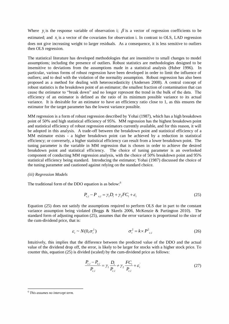
(iii) Regression Models

The traditional form of the DDO equation is as below:6

, , 1 2c i x i i i iP P D FC (25)

Equation (25) does not satisfy the assumptions required to perform OLS due in part to the constant

variance assumption being violated (Beggs & Skeels 2006, McKenzie & Partington 2010). The standard form of adjusting equation (25), assumes that the error variance is proportional to the size of

the cum-dividend price, that is:

2~ (0, )i iN

2 2

,i c ik P (26)

Intuitively, this implies that the difference between the predicted value of the DDO and the actual

value of the dividend drop off, the error, is likely to be larger for stocks with a higher stock price. To

counter this, equation (25) is divided (scaled) by the cum-dividend price as follows:

, , '

1 2

, , ,

c i e i i ii

c i c i c i

P P D FC

P P P

(27)

6 This assumes no intercept term.

Equation (27) is the standard choice of adjustment to the DDO equation which is used to mitigate the

impact of heteroscedasticity. Other variables identified in the literature influencing the error variance include market capitalisation (Hathaway & Officer 2004), dividend yield (Michaely 1991, Hathaway

& Officer 2004), and inverse stock return variance (Bellamy & Gray 2004). Intuitively, the dividend

yield results in heteroscedasticity as stocks with larger dividends will cause a larger price drop-off,

and as a consequence have a proportionally larger error. Stock price return variance refers to the historical volatility of the stock. A stock that is historically volatile over a long period of time is likely

to have a larger error variance then a stock with low historical volatility, regardless of the size of the

dividend paid. As a consequence a measure of historical stock return volatility is required in order to reduce this form of heteroscedasticity.

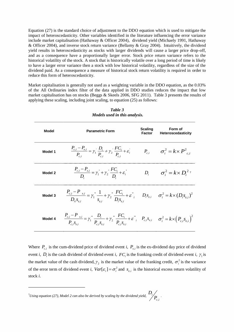
Market capitalisation is generally not used as a weighting variable in the DDO equation, as the 0.03%

of the All Ordinaries index filter of the data applied in DDO studies reduces the impact that low market capitalisation has on stocks (Beggs & Skeels 2006, SFG 2011). Table 3 presents the results of

applying these scaling, including joint scaling, to equation (25) as follows:

Table 3

Models used in this analysis.


Form of Heteroscedasticity

Model 1 , , ' ' '

1 2

, , ,

c i e i i ii

c i c i c i

P P D FC

P P P

,c iP 2 2

,i c ik P

Model 2 , , '' '' ''

1 2

c i x i ii

i i

P P FC

D D

iD 2 2

i ik D 7

Model 3 , , ''' ''' '''

1 2

, , ,

1c i x i ii

ii e i e i i e i

P P FC

D s s D s

,i e iD s

2 2

,( )i i e ik D s

Model 4 , , '''' '''' ''''

1 2

, , , , , ,

c i x i i ii

c i e i c i e i c i e i

P P D FC

P s P s P s

, ,c i e iP s

22

, ,i c i e ik P s

Where ,c iP is the cum-dividend price of dividend event i, ,x iP is the ex-dividend day price of dividend

event i, iD is the cash dividend of dividend event i, iFC is the franking credit of dividend event i, 1 is

the market value of the cash dividend, 2 is the market value of the franking credit, 2

i is the variance

of the error term of dividend event i, 2[ ]i iVar and ,e is is the historical excess return volatility of

stock i.

7Using equation (27), Model 2 can also be derived by scaling by the dividend yield, ,

i

c i

DP

.

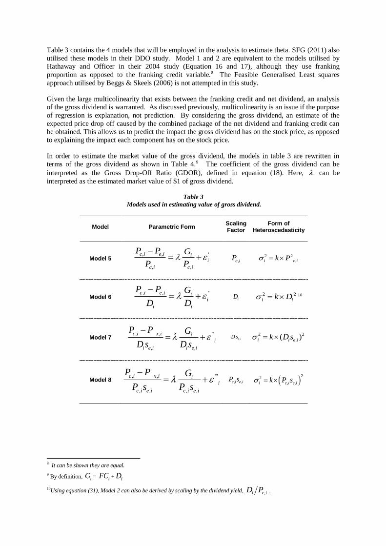
Table 3 contains the 4 models that will be employed in the analysis to estimate theta. SFG (2011) also

utilised these models in their DDO study. Model 1 and 2 are equivalent to the models utilised by Hathaway and Officer in their 2004 study (Equation 16 and 17), although they use franking

proportion as opposed to the franking credit variable.8 The Feasible Generalised Least squares

approach utilised by Beggs & Skeels (2006) is not attempted in this study.

Given the large multicolinearity that exists between the franking credit and net dividend, an analysis of the gross dividend is warranted. As discussed previously, multicolinearity is an issue if the purpose

of regression is explanation, not prediction. By considering the gross dividend, an estimate of the

expected price drop off caused by the combined package of the net dividend and franking credit can be obtained. This allows us to predict the impact the gross dividend has on the stock price, as opposed

to explaining the impact each component has on the stock price.

In order to estimate the market value of the gross dividend, the models in table 3 are rewritten in terms of the gross dividend as shown in Table 4.9 The coefficient of the gross dividend can be

interpreted as the Gross Drop-Off Ratio (GDOR), defined in equation (18). Here, can be

interpreted as the estimated market value of $1 of gross dividend.

Table 3

Models used in estimating value of gross dividend.


Form of Heteroscedasticity

Model 5 , , '

, ,

c i e i ii

c i c i

P P G

P P

,c iP

2 2

,i c ik P

Model 6 , , ''c i e i i

i

i i

P P G

D D

iD 2 2

i ik D 10

Model 7 , , '''

, ,

c i x i ii

i e i i e i

P P G

D s D s

,i e iD s 2 2

,( )i i e ik D s

Model 8 , , ''''

, , , ,

c i x i ii

c i e i c i e i

P P G

P s P s

, ,c i e iP s

22

, ,i c i e ik P s

8 It can be shown they are equal.

9 By definition, iG = iFC + iD

10Using equation (31), Model 2 can also be derived by scaling by the dividend yield, ,i c iD P .

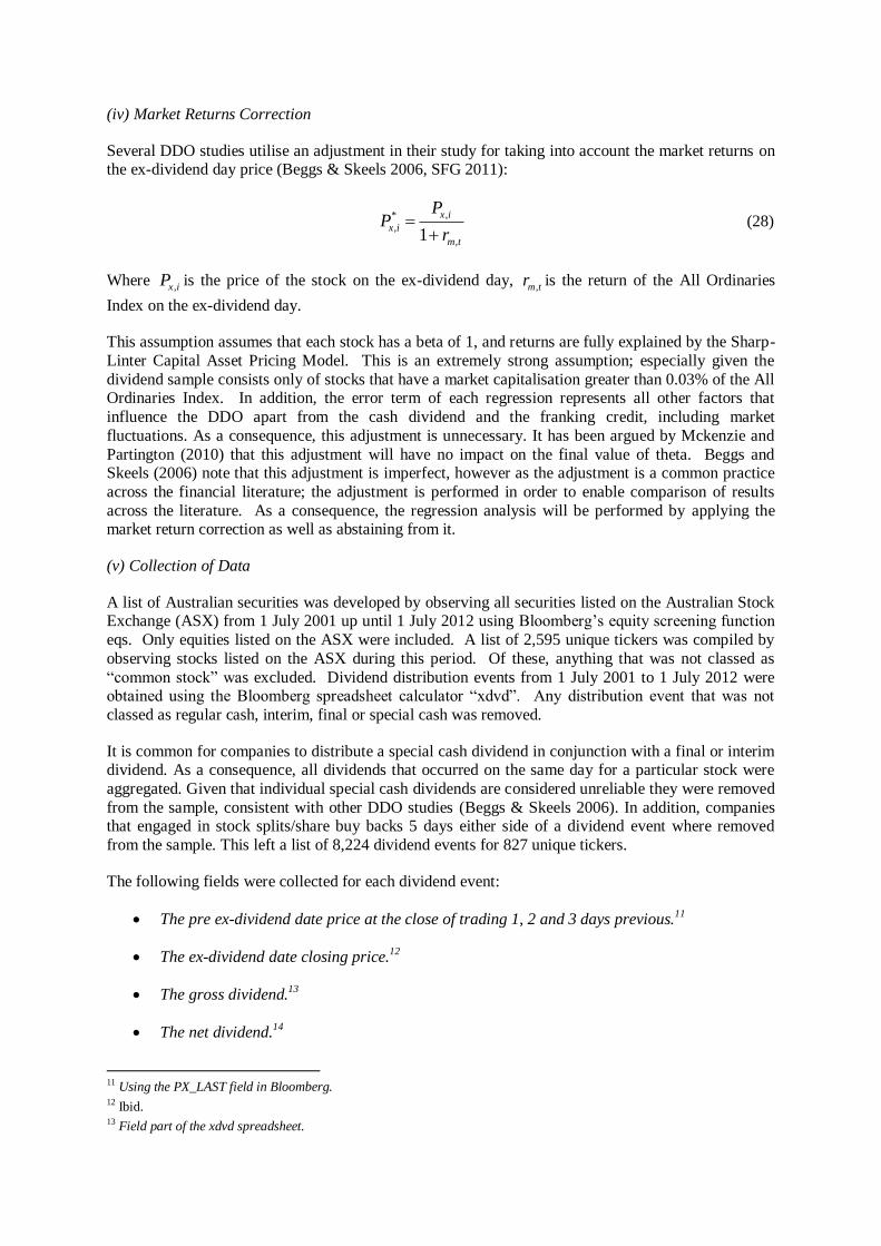
(iv) Market Returns Correction

Several DDO studies utilise an adjustment in their study for taking into account the market returns on the ex-dividend day price (Beggs & Skeels 2006, SFG 2011):

,*

,

,1

x i

x i

m t

PP

r

(28)

Where ,x iP is the price of the stock on the ex-dividend day,

,m tr is the return of the All Ordinaries

Index on the ex-dividend day.

This assumption assumes that each stock has a beta of 1, and returns are fully explained by the Sharp-

Linter Capital Asset Pricing Model. This is an extremely strong assumption; especially given the

dividend sample consists only of stocks that have a market capitalisation greater than 0.03% of the All Ordinaries Index. In addition, the error term of each regression represents all other factors that

influence the DDO apart from the cash dividend and the franking credit, including market

fluctuations. As a consequence, this adjustment is unnecessary. It has been argued by Mckenzie and

Partington (2010) that this adjustment will have no impact on the final value of theta. Beggs and Skeels (2006) note that this adjustment is imperfect, however as the adjustment is a common practice

across the financial literature; the adjustment is performed in order to enable comparison of results

across the literature. As a consequence, the regression analysis will be performed by applying the market return correction as well as abstaining from it.

(v) Collection of Data

A list of Australian securities was developed by observing all securities listed on the Australian Stock Exchange (ASX) from 1 July 2001 up until 1 July 2012 using Bloomberg’s equity screening function

eqs. Only equities listed on the ASX were included. A list of 2,595 unique tickers was compiled by

observing stocks listed on the ASX during this period. Of these, anything that was not classed as

“common stock” was excluded. Dividend distribution events from 1 July 2001 to 1 July 2012 were obtained using the Bloomberg spreadsheet calculator “xdvd”. Any distribution event that was not

classed as regular cash, interim, final or special cash was removed.

It is common for companies to distribute a special cash dividend in conjunction with a final or interim dividend. As a consequence, all dividends that occurred on the same day for a particular stock were

aggregated. Given that individual special cash dividends are considered unreliable they were removed

from the sample, consistent with other DDO studies (Beggs & Skeels 2006). In addition, companies that engaged in stock splits/share buy backs 5 days either side of a dividend event where removed

from the sample. This left a list of 8,224 dividend events for 827 unique tickers.

The following fields were collected for each dividend event:

The pre ex-dividend date price at the close of trading 1, 2 and 3 days previous.11

The ex-dividend date closing price.12

The gross dividend.13

The net dividend.14

11 Using the PX_LAST field in Bloomberg. 12 Ibid. 13 Field part of the xdvd spreadsheet.

The market capitalisation of the underlying stock on the ex-dividend date.15

The market capitalisation of the all ordinaries index on the ex-dividend date.16

The currency of the dividend event.17

The exchange rate for the dividend currency on the ex-dividend date. 18

The return of the All Ordinaries Index on the ex-dividend date.19

The cum-dividend price was calculated by observing the closing price of the relevant stock on the

trading day prior to the ex-dividend date. For example, if the ex-dividend date fell on a Tuesday, the cum-dividend price would be the closing price of the stock the previous Monday. A stock with an ex-

dividend date on Monday would have a cum-dividend date the previous Friday. The franking credit

for each dividend event is the residual between the gross dividend and net dividend. Any dividend event which had missing data was removed from the sample.

The sample was further reduced to include only companies that make up at least 0.03% of the All

Ordinaries index on the day of the ex-dividend date. This is consistent with other dividend drop off

studies (Beggs & Skeels 2006, SFG 2011). Any stock found to be paying a dividend denominated in currency other than the Australian dollar was converted to Australian dollars using the closing price

exchange rate on the ex-dividend date. The final sample contains 3,309 dividend events.

The stock return variance was estimated using a time series of each stocks historical prices, in addition to the historical value of the All Ordinaries Index. From this the daily returns of both the

stock and All Ordinaries Index was calculated. The daily excess return of the stock is defined as the

difference between the stocks daily return and the return of the All Ordinaries Index. The volatility of

the excess returns is calculated, over a year interval as follows:20

,, , 5

1

1( )

N

i ti t i t j

j

s er erN

is the estimated standard deviation of excess returns of stock i over N

trading days; , ,

1

1 N

i t i t

j

er erN

is the estimated mean of excess return of stock i over N trading

days; , , ,i t i t m t

er r r is the excess return of stock i over the market at time t ; ,i t

r is the daily return of

stock i at time t ; ,m t

r is the daily return of the All Ordinaries Index at time t .

This is the method employed by SFG (2011) in their DDO analysis when considering stock return volatility. This method allows for stocks volatility above the daily market fluctuations to be accounted

for, and as such it is adopted in this analysis. Our notation is slightly different to avoid confusion with

the variance of the error term.

14 Ibid. 15 Using the field in Bloomberg CUR_MKT_CAP. 16 Ibid. 17 Field part of the xdvd spreadsheet. 18 Using the PX_LAST field for the given currency. 19 Calculated by observing the price of the all ordinaries index on the ex-dividend day and the previous trading day using the

PX_LAST field in Bloomberg. 20 Calculated by observing all available excess returns within a one year interval, 5 days previous of the Ex-dividend date.

(vi) Summary of Data

The data from DDO studies can be summarised by considering the drop-off ratio, dividend yield and franking proportion of each dividend event. The drop-off ratio is calculated by the change in stock

price from the close of the cum-dividend day to the close of the ex-dividend day, divided by the

amount of the gross dividend. Dividend yield is calculated by the amount of the net dividend divided

by the stock price at the close of trading on the cum-dividend day. The franking proportion represents the fraction of dividends that have franking credits attached to them. A franking proportion of 1

indicates that the dividends are fully franked; a 0 franking proportion indicates no franking credits are

attached to dividends. Table 5 below summarises these variables in addition to the market capitalisation and volatility of excess returns21 for the dividend sample:

Table 4

Summary data of the dividend sample.

The histogram of the franking proportion is shown in Figure 1. This demonstrates the extreme multicolinearity present in DDO studies, as a large proportion of the sample of franking credits are

fully franked, approximately 75% of the entire sample. Recall that as the franking credit is a linear

function of the net dividend and franking proportion (13), a wide distribution of the franking proportion is a necessary condition for low correlation between the franking credit and net dividend.

Given the extreme distribution of the franking proportion below, we can conclude that this sample is

inflicted with severe multicolinearity. The extreme multicolinearity between the net dividend and franking credit is confirmed by the value of the Pearson Correlation, 0.81. As previously discussed, a

fully franked dividend does not contribute any information about the separate impact a net dividend

and franking credit has on the price drop off. As a consequence, only the 25% of the sample that is

not fully franked contains information that is used to distinguish the market value of the franking credit from the market value of the net dividend.

21 As described in paragraph 73. 22 Coal & Allied Industries paid a gross dividend of $0.36 on 28 Feb 2008, with the Cum-dividend price of $82 and an Ex-

dividend price of $100. 23 NewCreast mining paid a gross dividend of $0.20, with the price falling from $36.10 from the cum-dividend day to $32.86

on the ex-dividend day.

Drop-off

Ratio

Dividend

Yield

Franking

Proportion

Market

Cap%

Volatility of

excess returns

(daily)

Net

Dividend Franking Credit

Mean 0.56 0.02 83.2% 0.57% 0.019 $0.27 $0.073

Median 0.70 0.02 1 0.13% 0.018 $0.10 $0.037

Standard

deviation 1.81 0.013 0.34 1.55% 0.0076 $3.35 $0.20

Minimum -50.422 0.0001 0 0.03% 0.0061 $0.0025 $0.00

Maximum 16.223 0.14 1 16.9% 0.11 $140 $9.65

Figure 1

Frequency distribution of franking proportion

Whilst it is difficult to visualise multivariate data for Models 1 to 4, we can gain a general overview of the data by plotting the price drop off against the gross dividend, divided by the appropriate scaling

factor. This corresponds to a visualisation of Models 5 to 8. The graph of the relevant variables is

shown below:

Figure 2

Scatter plot of price drop-off against gross dividend, scaled by cum price (Model 5)

Histogram of Franking Proportion

Franking Proportion

Fre

quen

cy

0.0 0.2 0.4 0.6 0.8 1.0

050

010

0015

0020

0025

00

Figure 3

Scatter plot of price drop-off against franking credit, scaled by net dividend (Model 6)

Figure 4

Scatter-plot of price drop-off against gross dividend, scaled by net dividend and volatility (Model 7)

Figure 5

Scatter-plot of price drop-off against gross dividend, scaled by cum-price and volatility (Model 8)

Figure 2, 4 and 5 demonstrates that a positive relationship exists between the price drop-off ratio and

the gross dividend when scaled by the applicable variable. This is to be expected, given the empirical

results of the literature attributing a positive value to both the net dividend and franking credit. It is however hard to decipher a positive relationship between the price drop-off ratio and the gross

dividend when scaling by the net dividend, as illustrated in Figure 3.

Figure 3 reveals the extreme clustering of the data found when using model 2. The dependent variable can be expressed as:

.1

.1

ci i

i c ci

i i c

tD f

FC t tf

D D t

(29)

As the tax rate is constant, the dependent variable in model 2 is a linear function of the franking

proportion, if . Given that the franking proportion is between 0 and 1, clustered around whole

percentages, this results in model 2 being clustered, explaining the clustering found in figure 3.

Clustering of this form is undesirable in regression as it results in high standard errors of the estimated coefficients, in addition to being sensitive to the observations present.

(vii) Statistical Packages Used

The R statistical package has been used in order to implement the required regression methodologies. OLS was performed using the lm() function which is built into R.24 Robust regression was performed

using the rlm() function found in the MASS package, using the MM regression setting, with all

options set to default.25 Least absolute deviations regression was applied using the rq() function in the quantreg package, using a value of tau=0.5. 26

24 lm() function documentation can be found at: http://127.0.0.1:20803/library/stats/html/lm.html. 25 rlm() function documentation can be found at: http://127.0.0.1:20803/library/MASS/html/rlm.html. 26 rq() function documentation can be found at: http://127.0.0.1:20803/library/quantreg/html/rq.html.

(V) Results

The results of applying OLS, LAD and MM robust regression to the data set using the models in Tables 3 and 4 are shown below. It is noted that no weight is placed on the results derived from

applying OLS to the various models, due to the assumptions for OLS not being met. However, as

other DDO studies have utilised OLS it is included for comparison.

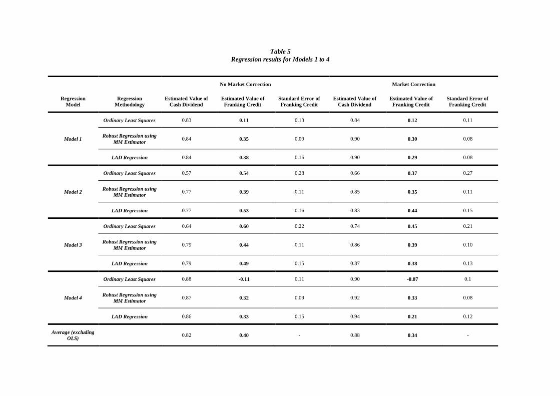
Table 5

Regression results for Models 1 to 4

No Market Correction Market Correction

Regression

Model

Regression

Methodology

Estimated Value of

Cash Dividend

Estimated Value of

Franking Credit

Standard Error of

Franking Credit

Estimated Value of

Cash Dividend

Estimated Value of

Franking Credit

Standard Error of

Franking Credit

Model 1

Ordinary Least Squares 0.83 0.11 0.13 0.84 0.12 0.11

Robust Regression using

MM Estimator 0.84 0.35 0.09 0.90 0.30 0.08

LAD Regression 0.84 0.38 0.16 0.90 0.29 0.08

Model 2



MM Estimator 0.77 0.39 0.11 0.85 0.35 0.11

LAD Regression 0.77 0.53 0.16 0.83 0.44 0.15

Model 3



MM Estimator 0.79 0.44 0.11 0.86 0.39 0.10

LAD Regression 0.79 0.49 0.15 0.87 0.38 0.13

Model 4

Ordinary Least Squares 0.88 -0.11 0.11 0.90 -0.07 0.1


MM Estimator 0.87 0.32 0.09 0.92 0.33 0.08

LAD Regression 0.86 0.33 0.15 0.94 0.21 0.12

Average (excluding

OLS) 0.82 0.40 - 0.88 0.34 -

Table 6

Regression results for Models 5 to 8


Regression Model Regression Methodology Estimated Value of Gross

Dividend

Standard Error of Gross

Dividend

Estimated Value of Gross

Dividend

Standard Error of Gross

Dividend

Model 1

Ordinary Least Squares 0.63 0.01 0.65 0.01

Robust Regression using MM

Estimator 0.68 0.01 0.73 0.01

LAD Regression 0.70 0.01 0.73 0.01

Model 2



Estimator 0.68 0.01 0.71 0.01

LAD Regression 0.70 0.01 0.72 0.01

Model 3



Estimator 0.69 0.01 0.73 0.01

LAD Regression 0.70 0.01 0.73 0.01

Model 4



Estimator 0.72 0.01 0.76 0.01

LAD Regression 0.70 0.01 0.73 0.01

Average (excluding

OLS) .70 - 0.73 -

The robust MM estimation method produces an estimate of the franking credit between 0.32 to 0.44,

whilst applying the market correction produces a robust MM estimation of between 0.30 to 0.39. LAD regression produces an estimate of the franking credit between 0.33 to 0.53 and using the market

correction produces estimates between 0.21 to 0.44.

With the exception of OLS, the results of applying robust MM regression and LAD regression to the

gross dividend models show only a small variation, between 0.68 and 0.72. The variation between the models and regression types for the estimated value of the gross dividend is considerably less than the

variation in the estimated value of the franking credit.

Whilst not directly comparable, the standard error of the estimate of theta tends to be lower for robust MM regressions than for LAD regressions. Producing estimates of confidence intervals and p-values,

as is standard in statistical analysis, is not appropriate for LAD and MM regression. Doing so

requires strong assumptions on the asymptotic distribution of the regression coefficients and standard

errors, which could give misleading results. The coefficient of determination, 2R , quoted in other

dividend drop off studies is also inappropriate as a measure of model reliability given that OLS models will always maximise this statistic. However, as OLS is inappropriate in DDO studies, the

coefficient of determination is also inappropriate as a measure of model reliability. Variance inflation

factors are also quoted when data is inflicted with multicolinearity, in order to gauge the impact

multicolinearity has on the estimated regression coefficients. Given that this is only appropriate for OLS models, variance inflation factors are not calculated.

The improved confidence in the estimation of the market value of the gross dividend over the franking

credit can be seen by the comparatively smaller standard errors of the regression coefficients. This confirms the impact of multicolinearity; on average we expect $1 of gross dividend to cause a

reduction in price from the cum-dividend price to the ex-dividend price of $0.70. However it is

difficult to isolate the contribution of the net dividend and the franking credit to the price-drop off, with the market value of the franking credit varying substantially between models and regression

procedures employed.

Interestingly, the use of the market correction results in a significant reduction in the estimate of theta,

contradicting Mckenzie and Partington (2010) and the analysis conducted by Skeels (2009) in analysis of SFG’s first report. The market value of the gross dividend generally increases upon application of

the market correction.

(VI) Sensitivity Analysis

(i) DFBETAS

It is undesirable that the estimates of theta show considerable variation across the different models.

This variation is compounded further if the market correction is utilised. It is valuable to investigate the impact on the estimate of theta on removing significant observations from the data set. This

analysis was performed in order to ascertain the sensitivity of the estimates to changes in the

underlying sample of dividend events.

As noted previously, DDO studies are extremely sensitive to the choice of the underlying sample of dividend events. As a consequence, it is necessary to use a statistical criterion in order to assess the

impact that each observation has on the estimated value of theta. In particular, how would removing a

specific dividend event impact the estimated value of theta? The DFBETAS criterion is appropriate as by definition chooses the point that has the most impact on the value of a regression coefficient. It

is also applicable across a range of different regression methodologies, unlike other criterions such as

Cooks Distance.

DFBETAS is a standardised measure of the amount by which a regression coefficient changes if a

particular observation is removed. Formally, ,DFBETASi k

is the standardised measure of the amount

by which the thk regression coefficient changes if the

thi observation is omitted from the data set

(Harell 2011):

( )

,

( )

DFBETAS( )

k k i

i k

k iSE

(30)

Where k is the thk regression coefficient from regressing on the entire data set; ( )k i is the

thk

regression coefficient by removing the thi observation;

( )( )k iSE is the standard error of the regression

coefficient by removing the thi observation.

Within the context of DDO studies, DFBETAS measures the standardised change in the estimated

value of theta by deleting the thi dividend event from the sample. Removing the observation with the

highest absolute value of DFBETAS will result in the largest change in the estimated value of theta.

It is desirable that the final estimate of theta would be robust to the removal of observations based on

this criterion. The sensitivity analysis is also performed to the gross dividend models in Table 4. Here, DFBETAS measures the standardised change in the estimated market value of the gross dividend, by

deleting the thi dividend event from the sample.

The sensitivity analysis was performed by removing the observation with the largest absolute

DFBETAS value, then refitting the model and observing the new estimate of the market value of franking credit. Due to the extremely high computational intensity of the DFBETAS statistic, 30

observations is seen as an appropriate cut-off for studying the robustness of the estimated value of

theta. The result of this sensitivity analysis for removing 30 observations is shown below. The result of applying this method is shown graphically in Appendix 2.

Table 8

Sensitivity analysis of value of franking credit

Regression

Model Regression Methodology

Minimum Value of

Franking Credit

Maximum Value of

Franking Credit

Mean Value of

Franking Credit

Median Value of

Franking Credit

Standard Deviation of

Franking Credit

Model 1

Ordinary Least Squares 0.11 0.33 0.21 0.19 0.065


MM Estimator 0.30 0.46 0.40 0.41 0.046

LAD Regression 0.34 0.49 0.41 0.39 0.05

Model 2



MM Estimator 0.36 0.47 0.41 0.41 0.033

LAD Regression 0.52 0.55 0.54 0.53 0.01

Model 3



MM Estimator 0.37 0.47 0.42 0.43 0.032

LAD Regression 0.38 0.52 0.48 0.49 0.053

Model 4

Ordinary Least Squares -0.11 0.37 0.18 0.18 0.14


MM Estimator 0.32 0.53 0.43 0.42 0.059

LAD Regression 0.30 0.33 0.32 0.32 0.015

Average

(excluding OLS) 0.36 0.48 0.42 043 -

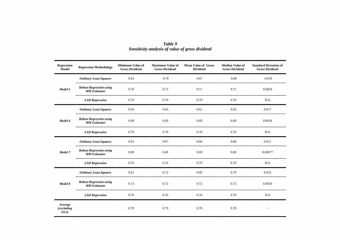
Table 9

Sensitivity analysis of value of gross dividend

Regression

Model Regression Methodology

Minimum Value of

Gross Dividend

Maximum Value of

Gross Dividend

Mean Value of Gross

Dividend

Median Value of

Gross Dividend


Gross Dividend

Model 5



MM Estimator 0.70 0.72 0.71 0.71 0.0054

LAD Regression 0.70 0.70 0.70 0.70 N/A

Model 6



MM Estimator 0.68 0.69 0.69 0.69 0.0034


Model 7



MM Estimator 0.69 0.69 0.69 0.69 0.00077


Model 8



MM Estimator 0.72 0.72 0.72 0.72 0.0020


Average

(excluding

OLS)

0.70 0.70 0.70 0.70 -

The results of the DFBETAS analysis confirm that the estimate of theta is highly sensitive to the

choice of the underlying sample of dividend events. Removing just 30 observations from a sample of 3309 can result in a dramatically different estimate of theta. In the course of this process, the value of

theta can vary between 0.3 to 0.55. It is important to note that these points represent less than 1% of

the entire dividend sample. Whilst by design the removed dividend event has the most extreme impact

on the estimate of theta it is undesirable for the estimate to be vulnerable to the removal of observations. Removing observations from a comparatively large sample in conjunction with the

robust regression techniques applied still produce estimates of theta that are unreliable.

The estimated value of the gross dividend is considerably more robust to the removal of observations than the estimated value of the franking credit. The removal of 30 observations from the sample of

3309 causes the estimated market value of the gross dividend to vary between 0.68 and 0.72.

(ii) Discussion of Robust Regression

The results of the sensitivity analysis highlight that despite the regression types being chosen for

being robust to influential points, removing observations from the sample results in a highly variable

estimate of theta. In addition, the results confirm a lack of consensus on the value of theta between

the different drop-off models and regression procedures employed.

The statistical literature notes that while the theoretical properties of MM regression are impressive, in

reality, its actual performance can be worse due to the theory being based on asymptotic large sample

theory (Olive & Hawkins 2008). In addition, MM regression is not robust to multicolinearity; it is only robust to the presence of outliers and heteroscedasticity. This lack of robustness to the sample

may be explained by the choice of tuning parameter and the trade-off between robustness and

statistical efficiency, as explained previously. Recall that in introducing the MM estimator, Yohai (1987) cautioned relying on the standard choice of the tuning parameter, a = 4.685. Applying a lower

tuning constant of a = 3.42, as opposed to a = 4.685 results in an 84.7% asymptotic efficiency and a

higher breakdown point. The results of applying MM regression with this tuning point are shown in

the tables below:

Table 7

MM regression results using a tuning constant of 3.42


Regression

Model

Estimated

Value of

Cash

Dividend

Estimated

Value of

Franking

Credit

Standard

Error of

Franking

Credit

Estimated

Value of Cash

Dividend

Estimated

Value of

Franking

Credit

Standard

Error of

Franking

Credit

Model 1 0.82 0.43 0.090 0.91 0.31 0.084

Model 2 0.80 0.418 0.11 0.88 0.32 0.104

Model 3 0.82 0.39 0.11 0.81 0.41 0.11

Model 4 0.83 0.43 0.09 0.92 0.33 0.08

Average 0.82 0.42 0.88 0.34

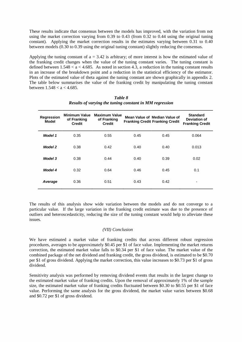
These results indicate that consensus between the models has improved, with the variation from not

using the market correction varying from 0.39 to 0.43 (from 0.32 to 0.44 using the original tuning constant). Applying the market correction results in the estimates varying between 0.31 to 0.40

between models (0.30 to 0.39 using the original tuning constant) slightly reducing the consensus.

Applying the tuning constant of a = 3.42 is arbitrary; of more interest is how the estimated value of

the franking credit changes when the value of the tuning constant varies. The tuning constant is defined between 1.548 < a < 4.685. As noted in section 4.3, a reduction in the tuning constant results

in an increase of the breakdown point and a reduction in the statistical efficiency of the estimator.

Plots of the estimated value of theta against the tuning constant are shown graphically in appendix 2. The table below summarises the value of the franking credit by manipulating the tuning constant

between 1.548 < a < 4.685.

Table 8

Results of varying the tuning constant in MM regression

Regression Model

Minimum Value of Franking

Credit

Maximum Value of Franking

Credit

Mean Value of Franking Credit

Median Value of Franking Credit


Franking Credit

Model 1 0.35 0.55 0.45 0.45 0.064

Model 2 0.38 0.42 0.40 0.40 0.013

Model 3 0.38 0.44 0.40 0.39 0.02

Model 4 0.32 0.64 0.46 0.45 0.1

Average 0.36 0.51 0.43 0.42 -

The results of this analysis show wide variation between the models and do not converge to a

particular value. If the large variation in the franking credit estimate was due to the presence of

outliers and heteroscedasticity, reducing the size of the tuning constant would help to alleviate these issues.

(VII) Conclusion

We have estimated a market value of franking credits that across different robust regression

procedures, averages to be approximately $0.45 per $1 of face value. Implementing the market returns correction, the estimated market value falls to $0.34 per $1 of face value. The market value of the

combined package of the net dividend and franking credit, the gross dividend, is estimated to be $0.70

per $1 of gross dividend. Applying the market correction, this value increases to $0.73 per $1 of gross dividend.

Sensitivity analysis was performed by removing dividend events that results in the largest change to

the estimated market value of franking credits. Upon the removal of approximately 1% of the sample size, the estimated market value of franking credits fluctuated between $0.30 to $0.55 per $1 of face

value. Performing the same analysis for the gross dividend, the market value varies between $0.68

and $0.72 per $1 of gross dividend.

The estimated market value of gross dividend is far more robust to the removal of significant

observations than the estimated market value of franking credits. This result indicates that two of the issues from DDO studies have been mitigated: (i) heteroscedasticity and (ii) the presence of outliers.

However, the application of robust regression techniques does not resolve the sensitivity of the

estimated value of theta to the underlying dividend sample. Taking the extreme position of

manipulating the tuning constant in robust regression does not reduce the sensitivity of the estimated value of theta. We can therefore conclude that it is not the presence of outliers or heteroscedasticity

that is the result of our imprecision; rather it is the strong multicolinearity between the franking credit

and the net dividend.

The extreme multicolinearity was demonstrated by the 0.81 Pearson correlation between the net

dividend and franking credit. Multicolinearity makes estimating the isolated impact correlated

variables have extremely difficult; however estimating the combined impact is relatively simple. This result can be seen in the above analysis. The value of franking credit and net dividend are extremely

sensitive to changes in the underlying sample, whilst the value of the gross dividend is relatively

robust. This implies that we can be relatively confident in predicting the price drop-off caused by both

the net dividend and franking credit in aggregate. However, we cannot be confident in our estimates of the relative effect the net dividend and the franking credit have on the price drop off in isolation.

The impact of multicolinearity has been demonstrated in the analysis by the high standard errors of

the regression coefficients relative to the standard errors of the gross dividend; and the extreme sensitivity of the franking credit estimate to changes in the underlying sample.

Other studies have removed observations based on “Price Sensitive” announcements around the ex-

dividend date, or removed outliers based upon an economic reasoning. This approach cannot reduce the imprecision of the DDO approach as extreme multicolinearity will still be present.

In estimating the value of theta for the WACC, the authors do not recommend using the results

derived from applying the market correction. Whilst market fluctuations will mask investor’s true

valuations of franking credits, they are accounted for by the error term in the regression models. Hence, applying the market correction is an unnecessary complication to an already complex

econometric task.

We have confirmed that estimating theta using the DDO methodology cannot give us a precise estimate for the value of theta. This result explains the large divergence and lack of consensus in the

economic and financial literature found in DDO studies in the past. In relation to the value of theta, it

may make sense to use a range for the value of theta rather than a derived point estimate. The

appropriate range suggested by this study is a value of theta between 0.35 to 0.55 based on the range of estimates encountered in the sensitivity analysis. If, however, a point estimate of theta is required,

then the estimated value of theta should be that based on an average across the robust regression

models, which is 0.45.

REFERENCES

Andersen, R. (2008), Modern Methods For Robust Regression. Thousand Oaks: SAGE Publications.

Australian Taxation Office, June 2012, Refunding Franking Credits, available at

http://www.ato.gov.au/individuals/distributor.aspx?menuid=0&doc=/content/8651.htm&page=4#P26

_3846.

Beggs, D.J. and Skeels, C.L. (2006), ‘Market Arbitrage of Cash Dividends and Franking Credits’, The

Economic Record, Vol. 82, No. 258, pp.239–252.

Bellamy, D. and Gray, S. (2004), “Using Stock Price Changes to Estimate the Value of Dividend

Franking Credits”, Working Paper, University of Queensland, Business School.

Berry, W.D. and Feldman, S. (1985) Multiple Regression in Practice, Sage Publications California,

p41.

Brown, P. and Clarke, A. (1993), ‘The Ex-Dividend Day Behaviour of Australian Share Prices Before

and After Dividend Imputation’, Australian Journal of Management.

Feuerherdt, C., Gray, S. and Hall, J. (2010), ‘The Value of Imputation Tax Credits on Australian

Hybrid Securities’, International Review of Finance, 10:3, p 365.

Harell F.E. (2001), Regression Modeling Strategies: With Applications to Linear Models, Logistic

Regression, and Survival Analysis Springer New York. p492.

Hathaway, N.J., and Officer, R.R. (2004), The Value of Imputation Tax Credits, working paper,

Melbourne Business School.

Huber, P.J (1996). Robust Statistical Procedures. Second edition. Philadelphia,:SIAM p1

McKenzie, M.D. and Partington, G. (2010), Selectivity and Sample Bias in Dividend Drop-Off

Studies (November 28) Finance and Corporate Governance Conference 2011 Paper. Available at

SSRN: http://ssrn.com/abstract=1716576 or http://dx.doi.org/10.2139/ssrn.1716576.

Michaely, R. (1991), “Ex-Dividend Day Stock Price Behavior: The Case of the 1986 Tax Reform

Act”, Journal of Finance.

Monkhouse, P. (1996) ‘The Valuation of Projects Under a Dividend Imputation Tax System’,

Accounting and Finance 36, pp.185-212.

Officer, RR (1994) - Accounting & Finance ‘The Cost of Capital of a Company Under an Imputation

Tax System’, p1-17.

Olive and Hawkins (2008) “The Breakdown of Breakdown” [Online]. URL:

http://www.math.siu.edu/olive/ppbdbd.pdf.

Principles of Econometrics (2008) Hill, Griffiths and Lim, John Wiley and Sons, p201.

SFG, Dividend drop-off estimate of theta, Final Report, 21 March 2011.

Skeels, C.L (2009) A Review of the SFG Dividend Drop-Off Study, The University of Melbourne.

http://www.math.siu.edu/olive/ppbdbd.pdf

http://www.math.siu.edu/olive/ppbdbd.pdf

Strategic Finance Group (SFG), The impact of franking credits on the cost of capital of Australian

companies, Report prepared for ENA, APIA and Grid Australia, October 2007, pp 35, 45.

Truong, G, and G. Partingon, 2006, ‘The Value of Imputation Tax Credits and Their Impact on the

Cost of Capital’, Accounting and Finance Association of Australia and New Zealand Conference,

Wellington.

Walker, S. and Partington, G. (1999), ‘The Value of dividends: Evidence from cum-dividend trading

in the ex-dividend period’, Accounting and Finance, Vol.39, pp.275–96.

Yohai, V.J. (1987), ‘High Breakdown-Point and High Efficiency Robust Estimates for Regression’,

The Annals of Statistics, Vol.15, No.2.

Appendix 1

Sensitivity analysis of theta estimating using DFBETAS criterion

Figure 6

Sensitivity analysis of Model 1 using OLS regression, observations removed through DFBETAS

criterion

Figure 7

Sensitivity analysis of Model 1 using MM Robust Regression, observations removed through

DFBETAS criterion

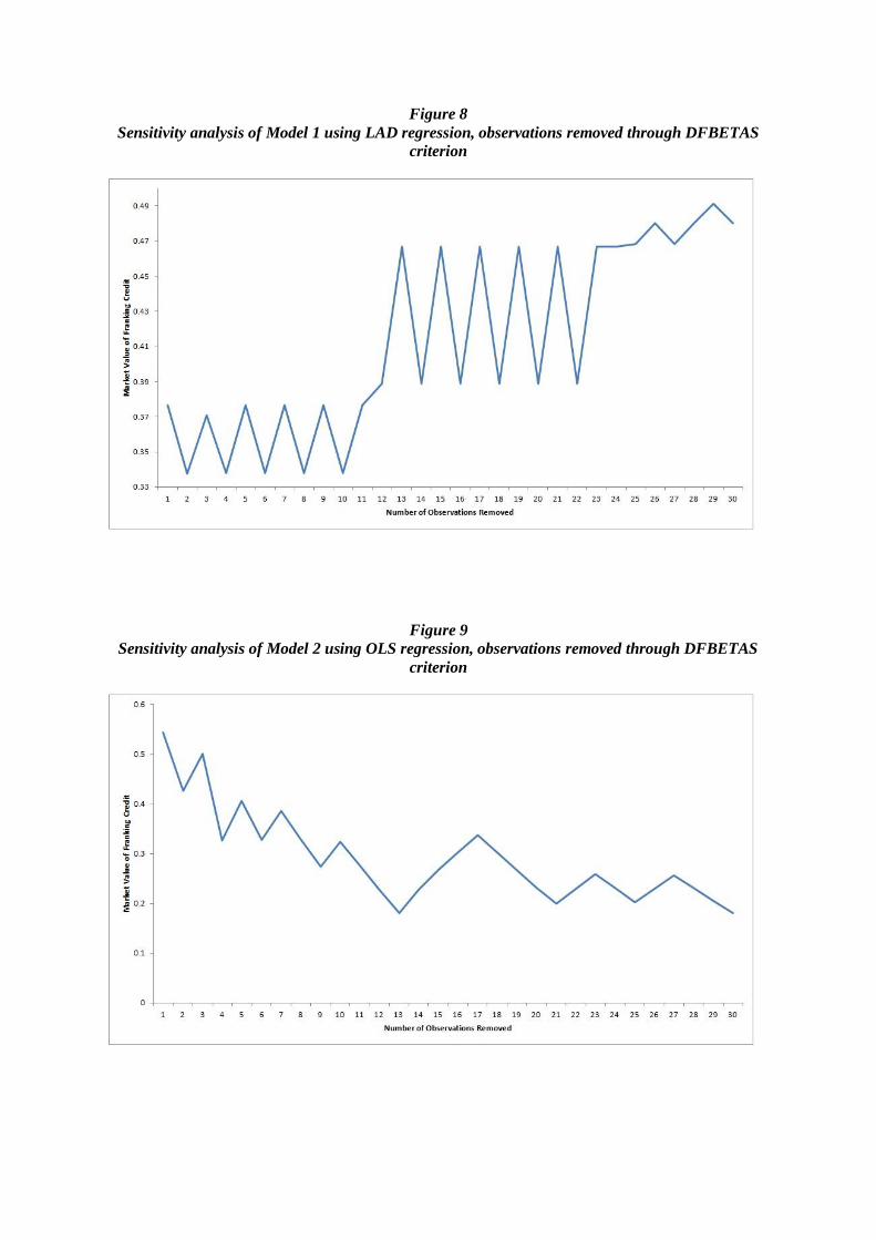
Figure 8

Sensitivity analysis of Model 1 using LAD regression, observations removed through DFBETAS

criterion

Figure 9


criterion

Figure 10

Sensitivity analysis of Model 2 using LAD regression, observations removed through DFBETAS

criterion

Figure 11

Sensitivity analysis of Model 2 using MM regression, observations removed through DFBETAS

criterion

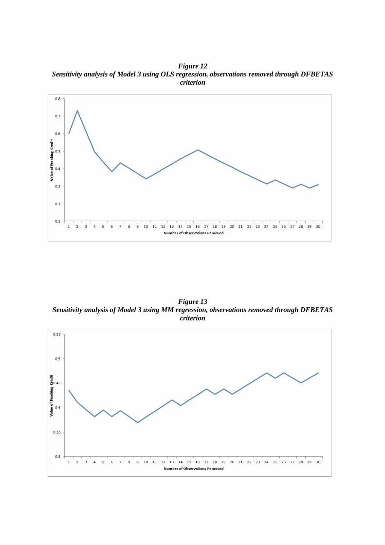
Figure 12


criterion

Figure 13


criterion

Figure 14


criterion

Figure 15


criterion

Appendix 2

Sensitivity analysis of theta to varying the tuning constant in MM regression

Figure 16

16Manipulating the tuning constant in MM robust regression for Model 1, value of theta

Figure 17

Manipulating the tuning constant in MM regression for Model 2, value of theta

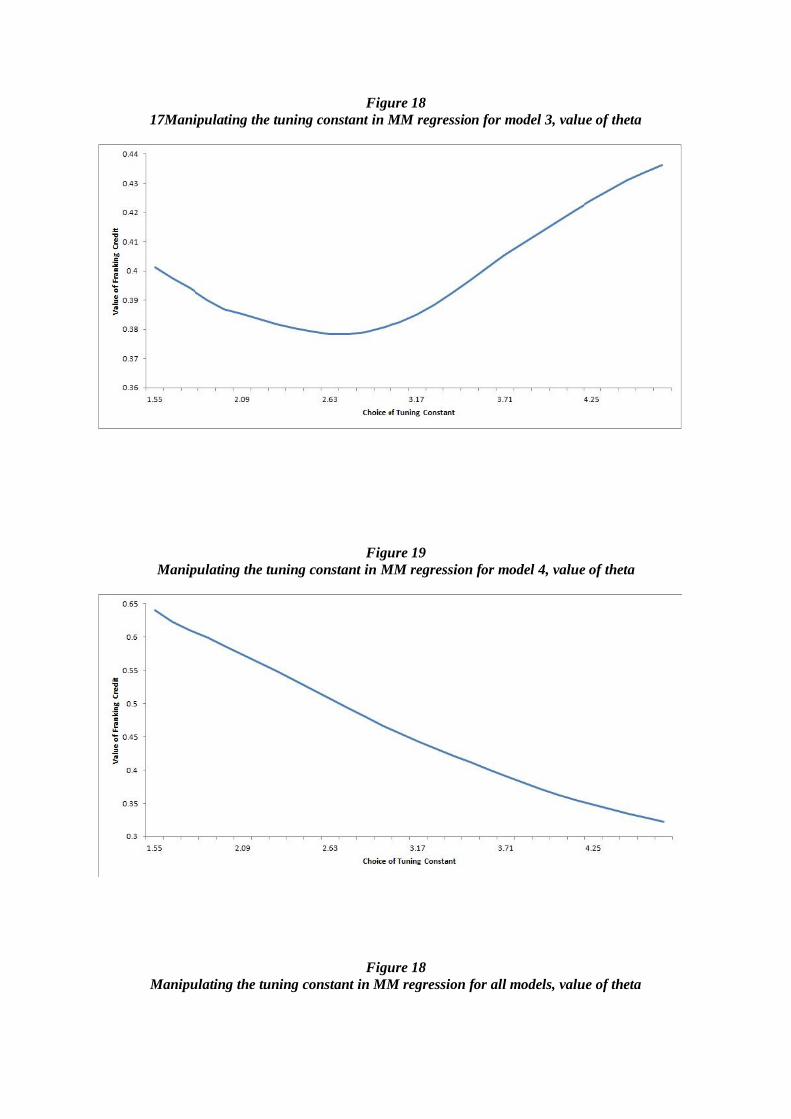
Figure 18

17Manipulating the tuning constant in MM regression for model 3, value of theta

Figure 19

Manipulating the tuning constant in MM regression for model 4, value of theta

Figure 18

Manipulating the tuning constant in MM regression for all models, value of theta

Documents

ESTIMATING THE MARKET VALUE OF FRANKING CREDITS: … · weighted average cost of capital in Australian regulatory decisions. There is, however, a lack of consensus on an appropriate