Embed Size (px)
Citation preview

ESTIMATING THE MEDICAL ULTRASOUND IN VIVO POWER SPECTRUM
BY
TIMOTHY ALLEN BIGELOW
B.S., Colorado State University, 1998 M.S., University of Illinois at Urbana-Champaign, 2001
DISSERTATION
Submitted in partial fulfillment of the requirements for the degree of Doctor of Philosophy in Electrical Engineering
in the Graduate College of the University of Illinois at Urbana-Champaign, 2004
Urbana, Illinois

ABSTRACT
This thesis considered the estimation of the in vivo power spectrum from the
backscattered waveforms by finding the total attenuation along the propagation path. The total
attenuation was estimated by assuming model for the scatterers (i.e., spherically symmetric
Gaussian impedance distributions of unknown size) and then solving for the size and total
attenuation simultaneously from the frequency dependence of the backscattered spectrum. The
attenuation and scatterer size could be accurately and precisely estimated provided that sufficient
frequency data was available. The accuracy and precision were significantly improved by
increasing the range of frequencies used in the estimate. In addition, some improvement could
be obtained by increasing the length of the window used to gate the backscattered RF echoes
(i.e., samples in frequency domain independent). Although only applied to the estimation of
scatterer size in this thesis, the estimation of the in vivo power spectrum using the developed
methods could be applied to other tissue characterization procedures as well as estimating the
temperature increase in the tissue from ultrasound exposures.
iii

ACKNOWLEDGMENTS First of all, I would like to thank my adviser, Dr. William O’Brien, for his help on this work. I
would also like to recognize my coworkers in the Bioacoustics Research Laboratory because of
help they provided during the investigation. Last of all, I want to reference Exodus 15:2 and 1
Corinthians 3:11-15.
iv
TABLE OF CONTENTS LIST OF SYMBOLS .................................................................................................................viii CHAPTER 1 INTRODUCTION TO THE IN VIVO ESTIMATION PROBLEM ....................... 1
1.1 Motivation: The Need to Know the In Vivo Power Spectrum .......................................... 1 1.2 Background: Previous Approaches ................................................................................... 3
1.2.1 Neglect patient variation .......................................................................................... 4 1.2.2 Total attenuation from the spatial decrease in backscattered intensity ................... 5 1.2.3 Total attenuation by ray method .............................................................................. 5
1.3 Approach and Summary of Results .................................................................................. 6 CHAPTER 2 THEORETICAL MODELING OF BACKSCATTER USING FOCUSED SOURCES ............................................................................................................................... 8
2.1 Derivation of Backscattered Voltage from Tissue Microstructure ................................... 9 2.2 Traditional Method to Obtain Scatterer Size .................................................................. 27 2.3 Chapter Summary ........................................................................................................... 29
CHAPTER 3 COMPARISON OF ATTENUATION-COMPENSATION FUNCTIONS ......... 30
3.1 Simulation Analysis of Gaussian Scatterers .................................................................. 31 3.2 Experimental Results for Glass Bead Scatterers ........................................................... 39
3.2.1 Equivalent Gaussian dimension measurement ...................................................... 39 3.2.2 Experimental procedure and results ....................................................................... 43
3.3 Simulation Results for Glass Bead Scatterers ................................................................ 47 3.4 Chapter Summary ........................................................................................................... 53
CHAPTER 4 GAUSSIAN TRANSFORMATION ALGORITHM ........................................... 56
4.1 Background Theory ........................................................................................................ 56 4.2 Determine Bandwidth and Center Frequency ................................................................. 58 4.3 Algorithm to Find Scatterer Size and Total Attenuation ................................................ 60
4.3.1 Compensating for Electronic Noise ....................................................................... 61 4.4 Simulation Results .......................................................................................................... 62 4.5 Chapter Summary ........................................................................................................... 65
CHAPTER 5 SPECTRAL FIT ALGORITHM .......................................................................... 67
5.1 Basic Spectral Fit Algorithm .......................................................................................... 67 5.1.1 Initial simulation results ........................................................................................ 68
5.2 Modifications to the Basic Spectral Fit Algorithm ......................................................... 75 5.2.1 Noise reduction techniques .................................................................................... 75 5.2.2 Windowing function compensation ....................................................................... 77 5.2.3 Updating frequency range used for fit ................................................................... 80
5.3 Chapter Summary ........................................................................................................... 83 CHAPTER 6 SIGNAL PROCESSING TECHNIQUES TO IMPROVE THE PRECISION
v
OF SPECTRAL FIT ALGORITHM .................................................................................... 84 6.1 Growing Window Averaging .......................................................................................... 84 6.2 Homomorphic Deconvolution ........................................................................................ 86 6.3 Averaging of Combinations ............................................................................................ 93 6.4 Varying Form Factor .................................................................................................... 100 6.5 Chapter Summary ......................................................................................................... 102
CHAPTER 7 EFFECT OF kaeff VALUES AND FREQUENCY RANGE USED IN ESTIMATION .................................................................................................................... 103
7.1 kaeff Range Results for the Spectral Fit Algorithm ....................................................... 103 7.1.1 Results for different source bandwidths .............................................................. 104 7.1.2 Results for different half-space attenuations ....................................................... 106 7.1.3 Results for different levels of electronic noise .................................................... 108
7.2 kaeff Range Results for the Traditional Algorithm ........................................................ 110 7.3 Initial kaeff Results for the Spectral Fit Algorithm ....................................................... 113 7.4 Chapter Summary ......................................................................................................... 122
CHAPTER 8 ANALYIS OF AVERAGE SQUARED DIFFERENCE SURFACES .............. 124
8.1 Properties of ASD Surfaces from Simulated Waveforms ............................................. 124 8.2 Mathematical Derivation and Analysis of Ideal ASD Surfaces .................................... 132
8.2.1 Derivation of ASD surface ................................................................................... 133 8.2.2 Analysis of ideal surfaces .................................................................................... 136
8.3 Relating Properties of the ASD Surfaces to Precision of Spectral Fit Algorithm ......... 145 8.4 Chapter Summary ......................................................................................................... 153
CHAPTER 9 CONCLUSIONS AND FUTURE WORK ......................................................... 155
9.1 Conclusions from Current Investigation ....................................................................... 155 9.2 Future Directions for In Vivo Power Spectrum Estimation .......................................... 158
9.2.1 Future work on size estimation ............................................................................ 158 9.2.2 Future work on other applications ....................................................................... 161
APPENDIX A: REVIEW OF THERMODYNAMICS ...................................................... 163
APPENDIX B: OVERVIEW OF HUMAN SKULL .......................................................... 166
APPENDIX C: DERIVATION OF THE BIOHEAT EQUATION ................................... 168 APPENDIX D: OVERVIEW OF SIMULATOR USED TO FIND BACKSCATTERED DATA ....................................................................................................... 178 APPENDIX E: COMPARE COMPLETE FIELD TO GAUSSIAN APPROXIMATION . 198 APPENDIX F: EXAMPLE AVERAGE SQUARED DIFFERENCE CONTOURS FOR SPECTRAL FIT ALGORITHM ................................................................. 208
vi

APPENDIX G: REFLECTION FROM A PLANE PLACED NEAR THE FOCUS AT ARBITRARY ANGLE ............................................................................... 216 REFERENCES .................................................................................................................... 237
VITA .................................................................................................................................... 243
vii

LIST OF SYMBOLS a = aperture radius for a spherically focused source.
A = term for form factor written as a power law.
Acomp = generalized attenuation-compensation function including focusing effects along the beam
axis.
aeff = effective radius of scatterer.
aeff j = estimated effective radius of scatterer found from one set (i.e. 25 averaged RF echos) of
simulated backscatter waveforms.
aeff = mean value of estimated effective radius from all sets of backscattered waveforms (i.e.,
a aeff eff jj j
=∀ ∀∑ ∑ j ).
AOO = Oelze-O’Brien attenuation-compensation function.
AOM = O’Donnell-Miller attenuation-compensation function.
APC = point attenuation-compensation function.
areal = real value for effective radius of scatterer when comparing to estimated value.
ASD = average squared difference value used when solving minimization.
ASDplane = average squared difference between theory and measurement for Plexiglas
experiment.
Aν = affinities associated with vibrational mode of ν -type molecules in fluid particle.
bγ = correlation function of individual scatterer.
Bγ = correlation function related to field and scatterers.
c = effective small-signal sound speed of medium.
C1,C2 = constants used in derivations.
cn = small-signal sound speed of region n.
co = small-signal sound speed of water.
cT = speed of sound assuming isothermal propagation.
cV = the specific heat at constant volume.
cVfr = the specific heat at constant volume when vibrational modes are not allowed.
cV eff = the effective specific heat at constant volume.
viii

cνν = specific heat at constant volume contribution from vibrational mode of ν -type molecules in
fluid particle.
d = characteristic length describing Gaussian impedance distribution.
dkn~ = difference between the effective complex wavenumber along the propagation path and the
complex wavenumber in a particular region (i.e., dk ). k kn n~ ~ ~= −
e = thermodynamic internal energy.
E = total energy of thermodynamic system.
E[], EN[] = expected value of term in brackets.
e j = unit vector defining coordinate system in thermodynamic calculations (j = 1, 2, or 3).
eν = thermodynamic internal energy associated with vibrational mode of ν -type molecules in
fluid particle.
f = frequency.
F = focal length for a spherically focused source.
f# = f-number for a spherically focused source (i.e., f F a#= 2 ).
fo = the frequency corresponding to the spectral peak of the Gaussian spectrum (i.e.,
exp −−FHG
IKJ
FHGG
IKJJ
f fo
2
2
σ ω
).
~fo = fo for backscattered spectrum modified by scatterer size.
′~fo = fo for backscattered spectrum modified by scatterer size and attenuation along propagation
path.
fpeak = frequency corresponding to the spectral peak at each inclination angle (i.e.,
Vf f
planepeak
p
∝ −−FHG
IKJ
FHGG
IKJJexp
2 2
2
σ ω
).
fR = the parameter used to set the location of the Rayleigh distribution along the frequency axis
(i.e., f f f R
R
⋅ −−FHG
IKJ
FHG
IKJ
expσ
2
).
FR = radiation force (i.e., F I cR loc= 2α ).
Fγ = form factor for scatterer.
ix
g r rd , ′b g = effective Green’s function valid from the scattering region to the detector.
Gcorr = windowing correction term for spectrum.
g r rn , ′b g
T g
= Green’s function for region n.
Go ,Go_trans = geometric gain value on receive/transmit for pressure field at focus when Wsource is
approximated by a Gaussian (units of m).
Gsp,Fsp,Λ= functions/variables used to find stationary phase solution to Green’s function for
planarly layered medium.
g r rT ′,b = Green’s function valid from the transmitter to the scattering region.
GT = dimensionless aperture gain function that accounts for the focusing of the ultrasound
source.
gwin = windowing function used to gate the signal.
Gwin = Fourier transform of gwin(t).
gwin2 = windowing function used for homomorphic filtering.
H = dimensionless filtering characteristics for the ultrasound source.
H01b g = 0th order Hankel function of the first kind.
I = temporal average intensity of ultrasound field.
I’ = instantaneous intensity of ultrasound field.
jo() = 0th order spherical Bessel function of the first kind.
Jo() = 0th order Bessel function of the first kind.
k = effective wavenumber along the propagation path. ~k = effective complex wave number along the propagation path (i.e. ~ ik k= + α ).
ko = wavenumber in water.
kn = wavenumber in region n (i.e., knn
=2πλ
).
~kn = complex wavenumber in region n (i.e., ~ in n= + αk k ). n
~knz = complex wavenumber in the z direction in region n (i.e., ~ ~k k ). knz n= −2 2ξ
KuV = conversion constant relating voltage to particle velocity for ultrasound source (units of m/s
V-1). ~ ,k kzs sξ = wavenumbers corresponding to stationary phase point.
x
kξ = wavenumber in the ξ-direction (i.e., k k kn nξ = − z~ ~2 2 ).
L = total width of windowing function.
Mimage = matrix used to generate image point.
n = average scatterer number density.
n = the outward unit normal on surface of the fluid particle.
N = last number in set of indices.
N(f) = additive electronic noise.
NdB = minimum value allowed for Nfloor when no electronic noise has been added.
nf = the outward normal for the plane at arbitrary angle to beam axis.
NFloor = noise floor of system used when selecting usable frequencies.
nI = vector perpendicular to the aperture plane of the image source.
Nlines = number RF echoes used when determining an estimate for Pscat.
p = pressure.
p’ = small perturbation to ambient pressure.
pinc = pressure field incident on the scatterers.
P P Pn p, , n = terms used to fit Gaussian distribution to spectrum in log domain.
po = ambient pressure.
pplane = pressure field from rigid plane placed near focal plane.
Pref =reference spectrum (i.e., P f k V Href o incb g b g b g= 4 2 4ω ω ).
ps = scattered pressure field.
Pscat = E V estimated from set of waveforms. refl
2
ptot = total pressure field (i.e., p p ptot s inc= + ).
q = the heat flow across the boundary of the fluid particle.
qblood = the heat removed by blood perfusion.
eQ = the rate heat flows into the thermodynamic system
qi = the heat generated within the fluid particle.
iQ = the rate heat is generated or removed internally for a thermodynamic system.
qsource = the heat generated by ultrasound source.
xi

r r r, ,′ ′′ = spatial locations in spherical coordinates.
∆r s, = change of spatial variables (i.e., ∆r r r= ′ − ′′ and s r r= ′ + ′′b g 2).
rf = locations on rigid reference plane in spherical coordinates.
rI = points on aperture plane of image source.
rmax = maximum distance off of beam axis used when comparing fields.
rn = location of single scatterer.
rs = location of point source in spherical coordinates.
r rT d, = locations on aperture plane of transmitter/detector in spherical coordinates.
Rγγ = autocorrelation function for the scatterer.
ℜγγ = power spectral density function for the scatterer.
′rρ = distance off of beam axis.
s = entropy.
S = strain tensor.
S = time derivative of S.
S* = surface of single fluid particle.
Sf = rigid plane near focal plane used to acquire reference waveform.
sfr = entropy associated with translational and rotational motions of fluid particle.
SI = aperture plane of image source.
SNR = signal-to-noise ratio.
ST = aperture plane of ultrasound transmitter.
sθ = variable used in substitution when evaluating integral.
sν = entropy associated with vibrational motions of fluid particle.
t = time.
T = temperature.
T’ = small perturbation to ambient temperature.
Tc = ambient temperature.
Tcep = value used to set the amount of homomorphic filtering.
Teff = effective temperature.
Termξ ,Term ,Te ,Term = terms describing ASD surface for Spectral Fit algorithm. aeffrmα aeffα ,
xii

Tij = transmission coefficient from region i to region j.
To = product of all transmission coefficients.
Twin = total width of windowing function applied to time-domain waveform (i.e., T L cwin = 2 ).
Tν = temperature associated with vibrational mode of ν -type molecules in fluid particle.
u = particle velocity.
uz = particle velocity perpendicular to aperture plane of ultrasound transmitter/detector.
′V = volume containing scatterers contributing to the scattered signal.
V* = volume of single fluid particle.
Vcepi = a RF echo expressed in cepstrum domain.
Vinc = voltage applied to the ultrasound source during transmit.
Vj = backscattered voltage spectrum for a single RF echo.
vnoise = example noise signal voltage in time domain (i.e., no signal transmitted by source).
Vplane = voltage from ultrasound source due to the backscatter from rigid plane near focus.
Vmeasured = voltage spectrum returned from Plexiglas experiment.
Vrefl = voltage spectrum from ultrasound source due to the backscatter from scatterers.
vrefl i = voltage of a RF echo in time domain.
Vs = average scatterer volume.
Vtheory = theoretical voltage spectrum for Plexiglas experiment.
w = energy per unit volume.
W = the rate work interacts with a thermodynamic system.
Wsource = term describing fall off of field in focal region (units of m2).
Wsource = magnitude of Wsource.
wx,wy,wz = equivalent Gaussian dimensions on receive of pressure field in focal region.
wxo,wyo = equivalent Gaussian beamwidths at center frequency of transducer.
wx_trans,wy_trans,wz_trans = equivalent Gaussian dimensions on transmit of pressure field in focal
region.
wzm wzb = linear fit parameters for wz (i.e., w w wz zm zb= ⋅ +λ ).
X X, = terms used in minimization scheme to solve for scatterer size.
xI,yI,zI = coordinate location of image point.
xiii
z,ξ = Cartesian coordinate system for planarly layered medium (i.e., ξ = +x y2 2 ).
,z ξ = unit vectors defining z,ξ axis.
zj = location of region boundaries in planarly layered medium (j = 1,2,3, ...).
zf = distance of rigid plane to the focal plane.
zo = offset in window placement due to errors in sound speed.
zoF = shift of the focus away from geometric focus at a particular frequency.
zp = distance from the focus that the beam axis intersects with the inclined plane.
zT, zd = distance of aperture plane of the ultrasound transmitter/detector to the focal plane.
ztrans = distance from transmit focus to receive focus.
α = effective attenuation along the propagation path.
αb = intercept term of attenuation assuming general linear frequency dependence (i.e.,
α α α= +o bf ).
αerror = error in attenuation associated with inclination angle of plane.
αloc = local absorption coefficient of medium.
αn = attenuation in region n.
αo = slope of attenuation assuming strict linear frequency dependence (i.e., α α= ⋅o f ).
(αozT)j = estimated attenuation along the propagation path for single data set.
α o Tzb g = mean value for attenuation along the propagation path from all sets of backscattered
waveforms (i.e., α αo T o T jj j
z zg b g=∀ ∀∑ jb ∑ ).
αreal = real value for attenuation along the propagation path when comparing to estimated value.
βtherm = the coefficient of thermal expansion.
γ = combined perturbation of density and compressibility (i.e., γ γ γκ ρr rb g b g b gr= − ).
γmax = largest value of γ for Gaussian impedance distribution.
γ o2 = mean squared variation in acoustic impedance per scatterer.
Γplane = reflection coefficient of plane.
γκ = local perturbation in the compressibility due to the scatterers (i.e., γκ κ
κκ rrsb g b g=
−).
xiv

γρ = local perturbation in the density due to the scatterers (i.e., γρ ρ
ρρ rr
rs
s
b g b gb g=
−).
δ() = Dirac delta function.
δij = Kronecker delta function.
θd = dilatation term (i.e., fractional increase in volume given by θ d S S S= + +11 22 33).
θ d = time derivative of θd.
θf,φf = angles describing orientation of plane with beam axis.
κ = compressibility of background medium surrounding scatterers.
κs = compressibility of scatterers.
κt = the thermal conductivity of the medium.
λ = wavelength.
λL ,µL = Lame’ constants.
λo= the wavelength corresponding to the spectral peak from the reference spectrum.
µ = the shear viscosity.
µB = the bulk viscosity.
ξ d = particle displacement.
ξs(f) = spectral variations due to random scatterer spacing.
ξ ξ ξx y, , z
z
= coordinate system for the image source.
, ,ξ ξ ξx y = unit normal vectors defining coordinate system for the image source.
ρ = density of background medium surrounding scatterers.
ρ’ = small perturbation to ambient density.
ρc = ambient density.
ρο = density of water.
ρn = density of region n.
ρs = density of scatterers.
σ = tensor representing the external forces acting on the fluid particle.
σ alower = percent deviation in values of scatterer size for sizes smaller than the mean size (i.e.,
a aeff j eff< ).
xv
σ aupper = percent deviation in values of scatterer size for sizes larger than the mean size (i.e.,
a aeff j eff> ).
σ σξf f2 , ,, ξ = terms describing the frequency dependence of ξs(f).
σg = the bandwidth term for the Gaussian distribution approximating the windowing function
(i.e., G fwin
f
gb g 2 2
2
2
∝−
e σ ).
σn = the average of the normal components of the stress tensor.
σR = the bandwidth term for Rayleigh distribution (i.e., f f f R
R
⋅ −−FHG
IKJ
FHG
IKJ
expσ
2
).
σ α lower = deviation in dB/MHz in values of attenuation for attenuations smaller than the mean
attenuation (i.e., α αo T j o Tz zb g<b g ).
σ α upper = deviation in dB/MHz in values of attenuation for attenuations greater than the mean
attenuation (i.e., α αo T j o Tz zb g>b g ).
σω = the bandwidth term for Gaussian distribution (i.e., exp −−FHG
IKJ
FHGG
IKJJ
f fo
2
2
σ ω
).
~σ ω = σω for backscattered spectrum modified by scatterer size.
σωp = Gaussian bandwidth for reflected voltage from inclined plane (i.e.,
Vf f
planepeak
p
∝ −−FHG
IKJ
FHGG
IKJJexp
2 2
2
σ ω
).
τcep = time values in cepstrum domain.
Φ = field term for scattered pressure field.
φcomp = complete velocity potential field for focused source.
φinc = incident field term for scattered pressure field.
φij = components of rate-of-shear tensor.
Φo = field term for reflected voltage.
Ψ = transmission term for scattered pressure field.
Ψo = transmission term for reflected voltage.
xvi

ω = radian frequency.
Ω ωb g,Cx,Cy,Cz,Ck,X1x,X1y,X1z,X2x,X2y,X2z,Xk,Y1x,Y1y,Y1z,Y2x,Y2y,Y2z,Yk, ′ ′′ ′Y Y Yz z2 2, , k = grouping of
terms to facilitate the derivation of the voltage returned form the inclined plane.
xvii
CHAPTER 1
INTRODUCTION TO THE IN VIVO ESTIMATION PROBLEM
Over the past several decades there has been an explosion of new medical imaging
modalities. Also, established technologies, such as X-ray, have opened up new imaging methods
such as CT scans that allow for even greater diagnostic potential. Due to the number of different
imaging techniques, an imaging system may not remain competitive in the clinical environment
if it only provides the clinician with a qualitative image showing the placement of the patient’s
tissue. Structure and/or function of the tissue in question must also be obtained to enhance the
detection and diagnosis of medical problems. In medical ultrasound, obtaining this type of
information is both directly and indirectly related to the estimate of the in vivo power spectrum
on a patient specific basis.
1.1 Motivation: The Need to Know the In Vivo Power Spectrum
In the past, medical ultrasound has distinguished itself in functional imaging by providing
real-time images of tissue motion. Furthermore, Doppler ultrasound allows measurements and
images to be made of blood flow, allowing the clinician to diagnose many different disease states
[Routh, 1996]. Also, the impact and use of Doppler ultrasound and related techniques will only
increase as microbubble contrast agents are introduced into the blood stream to assess perfusion
conditions in the brain, tumors, and other organs [Wilkening et al., 1999; Wilkening et al., 2000;
Simpson et al., 2001].
Although the benefits provided by Doppler ultrasound and related techniques are
significant, the increased exposure levels required introduce the potential for damaging
bioeffects [Barnett, 2001]. Of particular importance is the heating near the developing cranial
bone of the fetus because heating of the developing brain tissue could potentially result in long-
term neurological disorders. The heating is difficult to predict due to the nonlinear propagation
1
of the ultrasound in the embryonic fluid [Bacon and Carstensen, 1990] as well as the changing
absorption characteristics of the developing fetal skull [Barnett, 2001]. In the past, these heating
concerns have been addressed by requiring that the output levels be kept much less than that
anticipated to produce biologically significant temperature increases. However, allowing greater
output power levels would improve the diagnostic capability of the ultrasound system. As a
result, the FDA (Food and Drug Administration, Center for Devices and Radiological Health)
now allows the developing fetus to be exposed to nearly 8 times the traditional dose, provided
that the equipment provides a real-time output display of the potential risk [Barnett, 2001].
Unfortunately, the accuracy of the current estimates of temperature rise have been shown to be
poor [Barnett, 2001; Horder et al., 1998, Wojcik et al., 1999] due to uncertainties in the total
frequency-dependent attenuation along the propagation path (i.e., in vivo power spectrum) and
absorption coefficient. The absorption coefficient measures the rate at which energy is absorbed
by the medium as the wave propagates and is often assumed to be the same as the attenuation
coefficient for most tissues [NCRP, 1992]. The attenuation coefficient measures the rate at
which energy is lost from the wave (i.e., from both scattering and absorption) as the wave
propagates. Hence, knowing the in vivo power spectrum on a patient specific basis would
improve our estimates of temperature rise.
As well as using ultrasound to image function, many investigators have also attempted to
quantify the structure of the tissue from the ultrasound images. Quantifying the tissue
microstructure to aid in tumor diagnosis is of particular interest. Lizzi et al. [1983; 1997a]
pioneered some of this work by comparing the backscattered spectrum from ocular masses to a
reference spectrum in order to assess disease states. The tissue was then characterized by fitting
a line to the calibrated power spectrum, relative to the reference spectrum, and determining the
spectral slope (dB/MHz), the spectral intercept (dB, extrapolation to 0 MHz), and the midband fit
(dB, value of fit at center frequency) [Lizzi et al., 1997a]. Lizzi was successful due to the
negligible frequency-dependent attenuation along the propagation path leading to the ocular
mass. Hence, the changes in the calibrated backscattered spectrum were due entirely to the
microstructure of the ocular masses and were not influenced by the intervening tissue. Before
the scattering properties of embedded tumors can be estimated, the total frequency-dependent
attenuation along the propagation path (i.e., in vivo power spectrum) must be known on a patient-
specific basis [Lizzi et al., 1983].
2
While quantifying the size and acoustic concentration of scatterers within tissue has
historically been a popular method to quantify tissue structure, other methods such as
elastography, sonoelasticity, and acoustic radiation force impulse imaging (ARFI) are being
developed. In general, these methods involve applying a force to a region of tissue and then
using ultrasound to measure the resulting displacement. If the magnitude of the force is known,
the mechanical properties such as the Young’s modulus of the tissue can be measured. Of
particular interest is ARFI which involves using one acoustic signal to provide the force using
radiation force, and a second acoustic signal to measure the displacement [Nightingale et al.,
2000]. Assuming that the forcing field is a plane wave, the resulting radiation force would be
given by
F IcRloc=
2α , (1.1)
where I is the temporal-average intensity, αloc is the local absorption coefficient of the medium,
and c is the speed of sound in the medium [Nightingale et al., 2000]. Hence, in order for the
magnitude of the applied force to be known and the stiffness of the tissue quantified, both the
intensity (i.e., in vivo power spectrum after attenuation along propagation path) and the local
absorption must be estimated. Also, because the force in ARFI is applied using an acoustical
signal, there is a greater potential for temperature related bioeffects [Nightingale et al., 2000], so
ARFI could also benefit from accurate real-time in vivo temperature rise monitoring.
Clearly, many different aspects of medical ultrasound would benefit from accurate
estimates of the in vivo power spectrum. Hence, this investigation attempted to improve the
reliability and accuracy in making estimates of the power spectrum by estimating the attenuation
along the propagation path using algorithms that could be later implemented on a patient specific
basis.
1.2 Background: Previous Approaches
Due to the significance of estimating the power spectrum in vivo for many different
aspects of medical ultrasound, a wide variety of approaches have been used by previous
investigators. A description of the previous approaches along with a discussion of the
shortcomings of each approach is provided below.
3
1.2.1 Neglect patient variation
The most common approach in the past, especially with regard to estimating temperature
rise, is to assume that the attenuation with distance along the propagation path and the local
absorption at the location of interest are exactly the same for every patient that will ever be
imaged. This is the basis for the traditional Thermal Indices (TI’s), used to predict ultrasound-
induced heating, and the Mechanical Index (MI), used to estimate the potential for nonthermal
bioeffects [Abbott, 1999; AIUM/NEMA, 1998]. The indicators are found by measuring the
output of the ultrasound source in a water bath and then derating the measured values by 0.3
dB/cm/MHz to predict the in vivo power spectrum [Abbott, 1999]. The local absorption
coefficient is also assigned a value depending on whether or not bone is in the region of interest
[Abbott, 1999]. As a related issue, the current TI’s only predict the steady-state temperature
increase while neglecting the exposure time required to reach this increase. Hence, others have
proposed that the exposure time also be included when predicting the resulting temperature rise
for safety considerations [Lubbers et al., 2003; Nightingale et al., 2000]. Although most
common when predicting temperature increases, the neglecting of patient variability has also
been used in studies involving the characterization of tissue microstructure. Oelze and O’Brien
[2002b] assumed that the rat tissues always had an attenuation coefficient of 0.9 dB/cm/MHz
when forming their microstructure images of rat tumors.
The obvious problem with this approach is that the attenuation and absorption
coefficients between patients and between different locations in the same patient are not
constant. As an example, consider a study of 24 patients with nonviable, first trimester
pregnancies as reported by the AIUM [1993]. In the study, the measured attenuation coefficient
for the abdominal wall varied from 0.39 ± 0.25 dB/cm/MHz for patients with a full bladder to
0.57 ± 0.37 dB/cm/MHz for patients with an empty bladder. Hence, the potential exists for
patient variability as high as 0.8 dB/cm/MHz depending on the state of the patients’ bladder. In
another study that measured the ultrasound signals in vivo, the total attenuation along the
propagation path from the abdominal wall through the vagina was measured 90 different times
using 57 different subjects with empty bladders and 161 different times using 64 subjects with
full bladders [Siddiqi et al., 1999]. In this study, the total attenuation coefficient varied from 0.8
± 0.4 dB/cm/MHz for the empty bladder to 0.6 ± 0.3 dB/cm/MHz for the full bladder.
4
As well as the gross differences in attenuation along the propagation path that can occur,
there are also differences in the attenuation within the same tissue type between patients as is
evident in the results reported by Goss et al. [1980]. In two different studies reported by Goss,
the attenuation coefficient for human liver (typical of soft tissue) was reported at 0.7 ± 0.2
dB/cm/MHz and 1.32 ± 0.3 dB/cm/MHz. Hence, the attenuation coefficient in liver can vary by
more than 1.1 dB/cm/MHz. Likewise, in a study done by Wear [2001a], the slope of the
attenuation coefficient versus frequency of 16 human calcaneus bone samples was measured at
12.86 ± 4.79 dB/cm/MHz, further emphasizing the variability in attenuation coefficient in the
same tissue type.
1.2.2 Total attenuation from the spatial decrease in backscattered intensity
Another method for determining the total attenuation along the propagation path in the
past, hence the in vivo power spectrum, involved compensating for the spatial decrease in
backscattered intensity by varying the assumed attenuation until the noise-to-signal ratio of the
echo envelope peaks from the source to the depth of interest was minimized [He and Greenleaf,
1986]. The noise in this case was the standard deviation of the echo envelope peaks and the
signal was the mean value of the echo envelope peaks. In this way, a single attenuation
coefficient was determined for all the tissue along the propagation path. Obviously, the best
estimates would be obtained if the tissue were homogeneous. Heterogeneities in the tissue
would yield errors in the attenuation estimate. He and Greenleaf [1986] also mentioned that
their theory would break down in the presence of specular reflections arising from vessel walls.
Hence, it is unlikely that their technique would work robustly in a clinical setting.
1.2.3 Total attenuation by ray method
Another method for estimating the total attenuation along the propagation path and the
resulting in vivo power spectrum involved making estimates of the local attenuation throughout
the tissue region for every tissue type. Then, rays could be traced back from the region of
interest to the source. The total attenuation was then found by summing up the local attenuations
along each ray path [Lizzi et al., 1992; Sidney, 1997]. This algorithm suffers from two potential
pitfalls. First, it is difficult to determine the local attenuation near the surface of the ultrasound
source. Second, errors in estimating the local attenuation would be compounded as the rays
5
moved deeper into the tissue. Sidney [1997] was able to achieve good performance using this
approach in simulations, but he assumed that the local attenuation was known exactly when, in a
clinical setting, it would also need to be estimated.
1.3 Approach and Summary of Results
Clearly, the problem of determining the in vivo power spectrum has not been solved. In
fact, it could be argued that the problem has been largely ignored. During the course of this
investigation, an entirely new approach to estimate the in vivo power spectrum was implemented
by considering the physics of the backscattered waves while assuming a model for the intended
targets. Because the model for the targets is strongly dependent on the intended application for
the ultrasound, the work focused on the spectral estimates as they apply to quantifying the size of
the scattering microstructure (i.e., scatterer) for the purpose of tissue diagnosis. However, some
of the background work for predicting the temperature increase at the bone/brain boundary when
exposed to focused ultrasound is addressed in Appendices A, B, C, and G.
Before the estimation approach related to quantifying the tissue microstructure can be
discussed, the assumptions involving the backscatter need to be understood. The research did
not intend to validate any of the traditional assumptions, but rather improvements in tissue
characterization were made within the existing framework. However, the developed algorithms
still retained enough flexibility to be adapted if new discoveries require the modification of these
assumptions. The fundamental assumption when characterizing the backscatter from biological
tissues is that the scattering sites are randomly positioned throughout the tissue region of interest
without any multiple or coherent scattering, and the region of interest is within the focal region
for the ultrasound source [Insana et al., 1990]. Furthermore, it is assumed that the form of the
acoustical impedance, or form factor F for the scatterer, is known (i.e., model for the
intended targets) and that only one type of scatterer exists in the tissue region [Insana et al.,
1990]. One common form factor assumed for tissue is the Gaussian form factor where the
acoustical impedance of the scatterer falls off according to a Gaussian distribution [Oelze and
O’Brien, 2002a; Insana et al., 1990]. The Gaussian form factor could also be used to model
tissue containing a distribution of scatterer sizes about a common mean. Due to its past
popularity, the Gaussian form factor was used in all of our computer simulations modeling
tissue. In addition to these assumptions, the developed algorithms for estimating scatterer size
aeffγ ω ,d i
6
neglected the effects of focusing along the beam axis. Hence, before developing the algorithms
for estimating the scatterer size and attenuation along the propagation path, the equations were
rederived to allow for the focused sources used in modern clinical ultrasound.
Based on these assumptions and the associated physics of the backscattered signals, two
algorithms were proposed and evaluated regarding their ability to estimate the total attenuation
along the propagation path (i.e., in vivo power spectrum) and scatterer size simultaneously. The
first algorithm investigated assumed that the backscattered spectrum could be accurately
modeled as a Gaussian distribution, the total attenuation had a linear frequency dependence, and
the form factor for the scatterer had the form e where A is some known constant times the
scatterer size and n . With these assumptions, the Gaussian bandwidth of the backscattered
power spectrum is only affected by the scatterer size, and, after correction for the scatterer size,
the center frequency is only affected by the total attenuation. The algorithm yielded acceptable
results for attenuations less than 0.25 dB/MHz (i.e., 0.05 dB/cm/MHz), but higher values of
attenuation had very poor performance. The degradation in performance resulted from the
spectra not being a perfect Gaussian. As the attenuation was increased the Gaussian bandwidth
of the backscattered power spectrum was reduced by the attenuation. Hence, the scatterer size
estimates were corrupted at the higher values of attenuation.
− Af n
≥ 2
From the first algorithm, it was evident that the total attenuation and scatterer size needed
to be considered simultaneously. Hence, in the second algorithm, the total attenuation and
scatterer size were found using a two-parameter minimization routine over the entire spectrum
similar to the traditional algorithm used previously to find just the scatterer size [Insana et al.,
1990]. Furthermore, the algorithm made no assumptions about the backscattered spectra or the
frequency dependence of the attenuation. It only assumed that the frequency dependence and
form factor were known. The algorithm gave good accuracy and precision for the attenuation
estimate provided that a large enough frequency range (largest frequency minus smallest
frequency) was used in the minimization. Likewise, the algorithm gave good accuracy and
precision for the scatterer size estimate when the frequency range multiplied by the scatterer size
was sufficiently large.
7

CHAPTER 2
THEORETICAL MODELING OF BACKSCATTER USING FOCUSED SOURCES
Most of the previous models used to analyze the backscattered waveforms have assumed
plane waves incident on the scattering region (i.e., inside focal zone of weakly focused source)
while only considering diffraction effects in the transverse plane [Lizzi et al., 1983; Insana et al.,
1990; Lizzi et al., 1997a]. Diffraction effects along the beam axis have been neglected. Other
authors included a complete Green’s function description of the source when determining the
scattered field [Madsen et al., 1984; Insana et al., 1986; Wear et al., 1989; Chen et al., 1993].
In their calculations, they assumed that the excitation across the entire surface of the source was
known or could be accurately determined. They also assumed that the scatterers were a
sufficient distance from the source, and the field was approximately constant across the scatterer.
Unfortunately, the resulting equations were cumbersome and required precise knowledge of the
source’s excitation in order to solve for the required fields. As a result, it is difficult to use their
results when experimentally calibrating a focused source for the purpose of estimating scatterer
size. Furthermore, their analysis still does not provide analytical insight into the effects of beam
diffraction. Recently, Gerig et al. [2003] proposed using a reference phantom containing
spherical glass bead scatterers to obtain a reference spectrum that could potentially account for
focusing. However, the ability of the reference phantom technique to correct for focusing has
not been fully evaluated, and the reference phantom technique still does not provide any
analytical insight.
Due to these limitations, most investigators use large f-number transducers in their
backscatter analyses where diffraction effects along the beam axis can be neglected over the size
of the region of interest (i.e., time gated region). Reducing the length of the time gate to allow
for smaller f-number transducers while still ignoring diffraction effects is not feasible because
both the accuracy and precision of the scatterer size (effective radius of spherically symmetric
8
scatterer) estimates degrade when the window length is too small. This is potentially restrictive
in diagnostic imaging systems where smaller f-numbers may be desirable to improve the spatial
resolution of the quantitative ultrasound image. Hence, the purpose of this chapter is to allow for
the use of focused sources when quantifying the backscattered ultrasound waveforms before
addressing the problem of unknown attenuation along the propagation path.
In this chapter, the expected backscattered voltage from a region of randomly positioned
uniform scatterers is rederived without the plane wave approximation. Instead, it is assumed that
the velocity potential field near the focus can be accurately modeled as a three-dimensional
Gaussian beam while continuing to assume that the scatterers are at a sufficient distance from the
source, and the field is approximately constant across the scatterer. The analysis is also extended
to find the expected backscattered intensity through a planarly layered low-contrast attenuating
medium. After completing the theoretical derivations, the traditional approach for estimating the
scatterer size based on the model will be discussed. Throughout the analysis, the effects of shear
wave propagation are neglected in order to simplify the mathematical expressions.
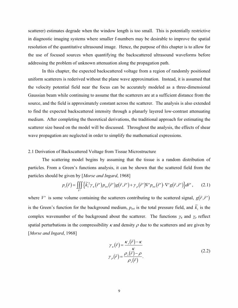
2.1 Derivation of Backscattered Voltage from Tissue Microstructure
The scattering model begins by assuming that the tissue is a random distribution of
particles. From a Green’s functions analysis, it can be shown that the scattered field from the
particles should be given by [Morse and Ingard, 1968]
p r k r p r g r r r p r g r r drs tot totV
b g b g b g b g b g b g b gn s= ′ ′ ′ + ′ ′∇ ′ ⋅ ′∇ ′′zzz ′~ , ,1
2γ γκ ρ , (2.1)
where ′V is some volume containing the scatterers contributing to the scattered signal, g r r, ′b g~
1
is the Green’s function for the background medium, ptot is the total pressure field, and k is the
complex wavenumber of the background about the scatterer. The functions γκ and γρ reflect
spatial perturbations in the compressibility κ and density ρ due to the scatterers and are given by
[Morse and Ingard, 1968]
γκ κ
κ
γρρ
κ
ρ
ρ
rr
rr
r
s
s
s
b g b g
b g b gb g
=−
=−
. (2.2)
9

In this equation, κs and ρs are the compressibility and density of the scatterers while κ and ρ are
the compressibility and density of the background medium. The effect of some variations in κ
and ρ in the background region can be captured by the Green’s function, so the only requirement
is that κ and ρ be approximately constant for some small volume about the scatterers.
At this point in the derivation, it is generally assumed that the medium away from the
scatterers is homogeneous resulting in the use of the homogeneous Green’s function [Gore and
Leeman, 1977; Lizzi et al., 1983; Nassiri and Hill, 1986; Insana et al., 1990]. This assumption is
not valid for biological tissue where the scattering region of interest is often buried beneath many
other tissue types. However, if we assume that multiple scattering between the layers can be
neglected, then the homogeneous Green’s function can be used with slight modification to
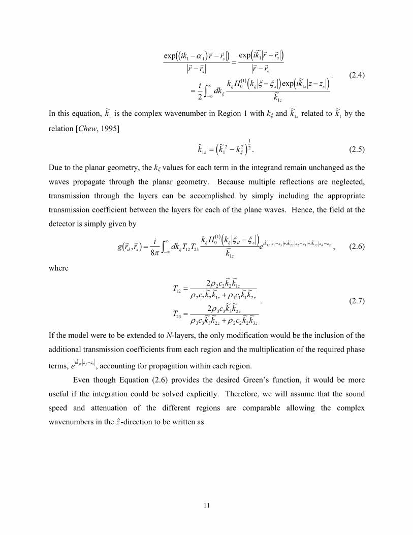
account for the sound transmission into the different layers. As an example, consider the
Green’s function for a point source imbedded in a planarly layered medium consisting of three
layers as shown in Figure 2.1.
Region 1
Region 2
Region 3
Source
Detector
z
z1
z2
ξ Figure 2.1: Planarly layered medium for Green’s function calculation where the boundaries
between the layers are defined as planes along the z-axis (z ) that are infinite in extent in the ξ-plane ( ). ξ
The “field” in Region 1 generated by the point source at location rs is given by [Morse
and Ingard, 1968]
g r rr r
ik r rss
s1 11
4 1, expb g b g=−
− −π
α , (2.3)
where k1 and α1 are the wavenumber and attenuation in Region 1. This field can then be
propagated through the other regions by decomposing it into a set of plane waves according to
[Chew, 1995]
10
exp exp ~
exp ~
~
ik r rr r
ik r r
r r
i dkk H k ik z z
k
s
s
s
s
s z
z
1 1 1
01
1
12
− −
−=
−
−
=− −
−∞
∞z
α
ξ ξξ
ξ ξ
b gc h d i
d i db gs i
. (2.4)
In this equation, ~k is the complex wavenumber in Region 1 with k1 ξ and ~k related to z1~k by the
relation [Chew, 1995] 1
~ ~k k kz1 12 2
12= − ξd i . (2.5)
Due to the planar geometry, the kξ values for each term in the integrand remain unchanged as the
waves propagate through the planar geometry. Because multiple reflections are neglected,
transmission through the layers can be accomplished by simply including the appropriate
transmission coefficient between the layers for each of the plane waves. Hence, the field at the
detector is simply given by
g r r i dk T Tk H k
ked s
d s
z
ik z z ik z z ik z zz s z z d, ~~ ~ ~b g d ib g
=−
−∞
∞ − + − + −z8 12 2301
1
1 1 2 2 1 3 2
π
ξ ξξ
ξ ξ , (2.6)
where
T c k kc k k c k k
T c k kc k k c k k
z
z
z
z z
122 2 2 1
2 2 2 1 1 1 1 2
233 3 3 2
3 3 3 2 2 2 2 3
2
2
=+
=+
ρρ ρ
ρρ ρ
z
~ ~~ ~ ~ ~
~ ~~ ~ ~ ~
. (2.7)
If the model were to be extended to N-layers, the only modification would be the inclusion of the
additional transmission coefficients from each region and the multiplication of the required phase
terms, eik z zjz j i~ − , accounting for propagation within each region.
Even though Equation (2.6) provides the desired Green’s function, it would be more
useful if the integration could be solved explicitly. Therefore, we will assume that the sound
speed and attenuation of the different regions are comparable allowing the complex
wavenumbers in the z -direction to be written as
11
~ ~ ~ ~ ~ ~ ~ ~ ~ ~
~ ~ ~ ~ ~ ~ ~
~ ~ ~~
~ ~ ~ ~~
~ ~ ~ ~~
~ ~ ~ ~~ ,
k k dk k k k dk k k k dk
k k k dk k kdk
dk kdkk
k k kdkk
k k kdkk
k k kdkk
z z z z z z z z
z z
zz
z zz
z zz
z zz
1 1 12 2
12 2
1
12 2
12
1
11
11
22
33
2 2
2 2
= + ⇒ ≅ + = − +
⇒ = + ≅ +
⇒ = ⇒ ≅ +
≅ +
≅ +
ξ z
(2.8)
where the dki~ are the differences from the approximate homogeneous value ~k in the complex
wavenumber for each layer (i.e., dk k ki i~ ~ ~= − ). Furthermore, keeping only the 0th-order
perturbations in the transmission coefficients since they are amplitude terms yields
T cc c
T cc c
122 2
2 2 1 1
233 3
3 3 2 2
2
2
≅+
≅+
ρρ ρ
ρρ ρ
. (2.9)
Substituting these values into the Green’s function then yields
g r r i T T dkk H k
ke ed s
d s
z
ik dkk
z z ik dkk
z z ik dkk
z zik z zz
sz z
dz d s, ~
~ ~~
~ ~~
~ ~~ ~b g d ib g
≅−
−∞
∞ − + − + −−z8 12 23
01 1
12
2 13
2
π
ξ ξξ
ξ ξ . (2.10)
The integral in Equation (2.10) can now be solved using the method of stationary phase
with [Chew, 1995]
g r r G k F k dk
G k i T Tk H k
ke
F k e
d s sp sp
spd s
z
i z z k
sp
i k dkk
z z k dkk
z z k dkk
z z
d s z
zs
z zd
, ,
, ~~
~ ~~
~ ~~
~ ~~
b g d i d i
d i d i
d i
b g
=
=−
=
−∞
∞
−
− + − + −FHG
IKJ
z Λ
Λ
ξ ξ ξ
ξξ ξ
ξ
π
ξ ξ
8 12 2301
11
22 1
32
. (2.11)
Under these conditions, the stationary phase point can be found at [Chew, 1995]
kk
z zs
d s
d s d s
ξ
ξ ξ
ξ ξ=
−
− + −
~
2 2. (2.12)
Hence, the integral for the Green’s function can be approximated to first order by
12
g r r F k G k dk
i T T ek H k
ke d
er r
T T e
d s sp s sp
i k dkk
z z k dkk
z z k dkk
z z d s
z
i z z k
ik r r
d s
i k dkk
z z k dkk
z
zss
zs zsd
d s z
d szs
szs
k
, ,
~~ ~
~~ ~
~~ ~
~ ~
~ ~ ~~
~ ~~
b g d i d i
d ib g
≈
=−
=−
−∞
∞
− + − + −FHG
IKJ −
−∞
∞
− − + −
zz
ξ ξ ξ
ξ ξξπ
ξ ξ
π
Λ
8
14
12 2301
12 23
11
22 1
32
11
22 z k dk
kz z
zsd1
32+ −
FHG
IKJ
~ ~~
,
(2.13)
where ~ ~k k kzs s= −2
ξ2 . (2.14)
Equation (2.13) can be further simplified by assuming that kξs is small compared to ~k as would
be the case for scattering regions located directly underneath the detector deep within the tissue.
With this assumption,
dkk
dk
kkk
dkk
kk
dkk
i
zs
i
s
i s i~
~~
~~
~~ ~
~~=
−
≅ +FHG
IKJ ≅
1
122
2
2
2ξ
ξ , (2.15)
yielding a Green’s function of
g r r er r
T T ed s
ik r r
d s
i dk z z dk z z dk z zd s
s d,~
~ ~ ~b g d≅−
−− + − + −1
4 12 231 1 2 2 1 3 2
πi . (2.16)
Therefore, the layered medium tends to modify the amplitude of the signal by the transmission
coefficients between the layers, and to modify the phase by a perturbation associated with the
distance spent within each layer. Based on this result, the optimal value of k is a weighted
average related to the distance covered by the wave within each layer.
~
Now that the appropriate Green’s function for the layered medium has been found,
Equation (2.1) can be solved to find the expected scattered field in Region 3. At this point, it
will be assumed that the scatterers of interest are weak scatterers that satisfy the Born
approximation. As a result, ptot can be replaced by only the incident field on the scatterers given
by [Morse and Ingard, 1968]
p r i u r g r r drinc z T T T TST
′ = − ′zzb g b g b g2 3ωρ , , (2.17)
13
where uz is the normal particle velocity at location rT on the aperture plane, ST, of the excitation
transducer. g r can be found by analysis similar to that used to find the Green’s function
in Equation (2.16) and is given by
rT ′,b gT
g r r er r
T T eT T
ik r r
T
i dk z z dk z z dk z zT
T′ ≅− ′
− ′− ′ + − + −,
~~ ~ ~b g d i1
4 21 321 1 2 2 1 3 2
π. (2.18)
Therefore, the scattered field at detector location rd is given by
p r i drk r u r g r r g r r
r u r g r r g r rdrs d T
S
z T T T d
z T T T dVT
b g b g b g b g b gb g b g b g b g= −
′ ′ ′
+ ′ ′∇ ′ ⋅ ′∇ ′
RS|T|
UV|W|zz zzz
′
2 312
ωργ
γκ
ρ
′~ , ,
, ,. (2.19)
Equation (2.19) can be further simplified by
′∇ ′ ≅ ′∇− ′
FHG
IKJ
=− ′
′∇ − ′> ′< ′
FHG
IKJ −
′∇ − ′−
− + −− ′ + − ′
− ′− ′ + − + −
g r r T T e er r
T T er r
e ik r r z idkz zz z
r rr
i dk z z dk z zik r r idk z z
ik r ri dk z z dk z z dk z z ∓
,
~ ~ ,
~ ~~ ~
~~ ~ ~
b g
d i
d i
d i
14
14
12 23
12 23 11
1
2 2 1 3 21 1
1 1 2 2 1 3 2
π
π ′
LNM
OQP
≅ ′ ′∇ − ′> ′< ′
LNM
OQP
r
g r r ik r r z idkz zz z
∓, ~ ~ , .b g d i1 1
1
(2.20)
Hence, ∇ becomes ′ ′ ⋅ ′∇ ′g r r g r rT T d,b g b , g
′∇ ′ ⋅ ′∇ ′ ≅′ ′∇ − ′ ⋅
′ ′∇ − ′
RS|T|
UV|W|
> ′< ′
≅ − ′ ′ ′∇ − ′ ⋅ ′∇ − ′
g r r g r rg r r ik r r z idk
g r r ik r r z idk
z zz z
k g r r g r r r r r r
T T d
T T T
d d
T T d T d
∓
∓, ,
, ~ ~
, ~ ~
~ , , ,
b g b gb g d ib g d i
b g b gc h c hn s
1
1
1
1
2
(2.21)
where once again, use has been made of the assumption that the perturbations in ~k between the
layers are small.
In order to make the above equations more tractable, the origin is placed within the
scattering region, and it is assumed that the dimensions of our scattering region are small relative
to its distance from the transducer and the detector. The validity of this approximation increases
with decreasing window length used to gate the signal in the time domain, increasing focusing
(i.e., decreasing f-numbers), and increasing focal length. In this case, the calculations are
simplified by [Morse and Ingard, 1968]
14

r r r x x y y z z r r r r r
rr
r r rr r
r r r rr
r
r r r rr
r
T T T T T T T
TT
TT T
T TT
T
d dd
d
− ′ = − ′ + ′ + ′ + ′ = − ⋅ ′ + ′
≅ − ⋅ ′ +′− ⋅ ′
FHG
IKJ ≅ − ⋅ ′
− ′ ≅ − ⋅ ′
2 2 2
2
2
2 42
2 2
1 12
12
b g b gb g b g
.
2
(2.22)
Also, assuming that the transducer and detector are in approximately the same direction (i.e.,
different elements of the same source), then
r rr rd T
d T
⋅FHGIKJ ≈ 1. (2.23)
Hence, Equation (2.21) becomes
′∇ ′ ⋅ ′∇ ′ ≅ − ′g r r g r r k g r r g r rT T d T T d ′, , ~ , ,b g b g b g b gn 2 s, (2.24)
yielding scattered field at the detector of
p r i dr u r g r r g r r k r k r dr
i k T T T T e er
dru r e e
rdr r
s d T z TS
T T dV
ikr idk z z idk z z
d
Tz T
ikr idk z z
T
T
d d
T T
b g b g b g b g b g b gn s
b g
b g b g
= − ′ ′ ′ − ′ ′
≅ −FHGIKJ ⋅
′ ′ −
zz zzz′
− + −
−
2
24
3 12 2
3
2
12 21 32 232 2 2 1 3 2
3 2
ωρ γ γ
ωρπ
γ γ
κ ρ
κ ρ
, , ~ ~
~ ~ ~ ~
~ ~
′FHGG
IKJJ
− ′ − ′⋅ +FHG
IKJ
′zzzzz r e
idk z z ikr rr
rr
VS
d
d
T
T
T
b gn s d i2 1 1~ ~
.
(2.25)
Equation (2.25) can also be generalized to an N-layered medium yielding
p r i k T T e T T e er
dr u r e er
dr r e
s d N j j j jidk z z
N N N Nidk z z
j
N ikr
d
T z Tidk z z
ikr
T
idk z z ikr rr
rr
V
j j j N d Nd
N T NT d
d
T
T
b g b g e j
b g b g d i
= −FHGIKJ ⋅
′ ′FHGG
IK
− −−
− −−
=
−
−− ′ − ′⋅ +
FHG
IKJ
′
− −
−
∏
zzz
24
2
1 12
1 12
1
2
1 1
11 1
ωρπ
γ
~, ,
~
, ,
~~
~~ ~ ~
JJ
= −FHGIKJ
zzS
N
ikr
dd d
T
d
i k er
k r k r24
2
ωρπ
b g d i d i~ ~, ~, ,
~
Ψ Φ
(2.26)
where
15
Ψ
Φ
~,
~,
, ,
~
, ,
~
~~ ~ ~
k r T T e T T e
k r dr u r e er
dr r e
dr r
d j j j jidk z z
N N N Nidk z z
j
N
d T z Tidk z z
ikr
T
idk z z ikr rr
rr
VS
j j j N d N
N T NT d
d
T
T
T
d i e j
d i b g b g
b
d i
=
= ′ ′FHGG
IKJJ
= ′ ′
− −−
− −−
=
−
−− ′ − ′⋅ +
FHG
IKJ
′
− −
−
∏
zzzzz1 1
21 1
2
1
2
1 1
11 1
γ
γ g d iφ inc
idk z z ikr rr
V
k r ed
d~,
~ ~
′FHG
IKJ
− ′ − ′⋅
′zzz 2 1 1
(2.27)
and
γ γ γ
φ
κ ρ′ = ′ − ′
′ =FHG
IKJ
−− ′⋅
−zzr r r
k r dr u r e er
einc T z Tidk z z
ikr
T
ikr rr
S
N T NT T
T
T
b g b g b g
d i b g~,~
~ ~1
. (2.28)
Before continuing the derivation of the scattered field, the analysis needs to be extended
to include detectors with finite dimension as opposed to the infinitesimally small point detectors
considered thus far. To simplify the analysis, the detector and source transducer will be the
same. It will also be assumed that the voltage across the transducer is directly related to the
normal particle velocity at the aperture plane according to the relations
u r K V G r H
VH
S Kdr u r G r
z T uV inc T T
reflT uV
d z d T dST
, ,
, , ,
ω ω ω ω ω
ωωω
ω ω
b g b g b g b g b gb g b g
b g b g b g=
= zz (2.29)
where Vinc is the voltage applied to the transducer, Vrefl is the voltage due to the backscatter, KuV
is the conversion constant relating voltage to particle velocity, H is the filtering characteristics
for the transducer, and GT is a gain function that accounts for the focusing of the source (i.e.,
concavity of the lens) that is defined at the aperture plane. As a result, the total voltage as
measured by the transducer is given by
VH
i S Kdr G r
p rz
k H
S Kdr G r
zer
k r k r
reflN T uV
d T ds d
dS
T uVd T d
dS
ikr
dd d
T
T
d
ωω
ωρ ωω
πω
ωω
b g b gb g b g b g
b g b gb g b g d i d i
=∂∂
=−FHGIKJ ∂
∂
FHG
IKJ
zz
zz
,
~
, ~, ~,~2
4
2
Ψ Φ
16
≅−FHGIKJ
′ ′ ′∂∂
F
HGGG
I
KJJJ
F
HGGG
I
KJJJ
− ′
′
− ′⋅
zzz zz2
4
2
2 1 1
b g b gb g b g d i b g d i
~
~, , ~,~
~ ~k H
S Kdr r k r e dr G r k r
ze
rT uVinc
idk z z
Vd T d d
dS
ikr ikr rr
dT
dd
dπω
ωγ φ ω Ψ
≅−FHGIKJ
′ ′ ′F
HGGG
I
KJJJ
− ′
′
− ′⋅
zzz zz2
4
2
22
1 1
i k kH
S Kdr r k r e dr G r k r z e
rT uVinc
idk z z
Vd T d d
d
ikr ikr rr
dS
dd
d
T
b g b gb g b g d i b g d i
~ ~~, , ~,
~
~ ~
πω
ωγ φ ω Ψ
(2.30)
because
∂∂
=∂∂
+ + =∂∂
+ + =rz z
x y zr z
x y z zr
d
d dd d d
d dd d d
d
d
2 2 2 2 2 212e j c h (2.31)
and
∂∂
− ′ =− ′
∂∂
− ′ + − ′ + − ′ =− ′− ′z
r rr r z
x x y y z zz zr rd
dd d
d d dd
dc h b g b g b ge j b g1
22 2 2 , (2.32)
yielding
∂∂
F
HGGG
I
KJJJ=
− ′− ′
FHG
IKJ −
≅ −
≅ ≅
− ′⋅
− ′ − ′
− ′− ′⋅
ze
re
r ikz zr r
zr
rzr
e r ik
ikzr
e ikzr
e
d
ikr ikr rr
d
ik r rd
d
d
d
d
d
d
d
ik r rd
d
d
ik r r d
d
ikr ikr rr
dd
dd d
dd
d
d
~ ~
~ ~
~~ ~
~~
~ ~.
b gd ie j2 3
2 2
1 (2.33)
Regrouping the appropriate terms in Equation (2.30) then yields
Vik V k k H
Sreflinc o o
T
ωω ω
πb g b g d i d i b g
b g≅−2
4
3 2
2
~ ~ ~Ψ Φ, (2.34)
where
Φ
Ψ
o sourceV
source T T T
ikr
T
ikr rr
S
idk z z
o j j j jidk z z
N N N Nidk z z
j
N
k dr r W k r
W k r dr G r er
e e
k T T e T T e
T T
T
T
j j j N T N
~ ~,
~, ,
~ .
~ ~~
, ,
~
, ,
~
d i b g d i
d i b g
d i e j
= ′ ′ ′
′ =FHG
IKJ
FHG
IKJ
=
′
− ′⋅− ′
− −−
− −−
=
−
zzzzz
∏ − −
γ
ω
2
2
1 12
1 12
2
1
1 1
1 1
(2.35)
17
Now that the scattered field at the detector location has been found given a known
arrangement of scatterers, the analysis needs to be extended for multiple randomly oriented
scatterers [Insana et al., 1990]. Because the position of the scatterers is random, the signal at the
detector over any given frequency range corresponds to a single realization of a random process
whose statistics are related to the properties of the scattering region. In order to see this
relationship, consider the second moment of the received voltage given by
E V V kS
H k V E k
kS
H k V dr drW k r W k r
E r r
refl reflT
o inc o
To inc
source source
VV
ω ωπ
ω ω
πω ω
γ γ
b g b g b g b g d i b g d i
b g b g d i b g d i d ib g b g
*
*
~ ~ ~
~ ~~, ~,
,
= LNM
OQP
= ′ ′′′ ′
′ ′′
FHGG
IKJJ
FHGG
IKJJ
′′zzzzzz
24
24
3
2
24 2 2 2
3
2
24 2 2
Ψ Φ
Ψ′
(2.36)
where ‘*’ is the complex conjugate and E[~] denotes expected value [Peebles, 1993].
In order to simplify Equation (2.36), the Wsource terms need to be simplified. Hence,
assume that the velocity potential field in the scattering region corresponds to a focused Gaussian
beam given by
dr u r er
G u z e e
G u z e
T z T
ikr ikr rr
TSo z T
xw
yw
zw ik zz r
o z T
xw
yw
zw
TT
T
T
x y zT
x y z
b g b g
b g
~ ~
~, ,
, ,
− ′⋅ −′FHGIKJ +
′FHGIKJ +
′FHGIKJ
FHGG
IKJJ − ′
−′FHGIKJ +
′FHGIKJ +
′FHGIKJ
FHGG
IK
F
HGGG
I
KJJJ≅
F
HGGG
I
KJJJ
≅
zz 0 0
0 0
2 2 2
2 2 2
JJ − ⋅ ′
F
HGGG
I
KJJJeik z z rT
~,b g
(2.37)
where wx, wy, and wz set the width of the focal region along the respective coordinate axes, Go is
the focusing gain for the transducer, and uz(0,0,zT) is the particle velocity at the center of the
aperture plane for the transducer. A similar assumption was shown to be valid in the focal plane,
i.e., z’=0, by Barber [1991]. For a spherically focused transducer, these quantities are
approximately given by [Kino, 1987; Barber, 1991]
FaGo 2
2
= (2.38)
and
w w f f wf
fx y z= = = = =0 51 2
20 87
354 22
6 012
2. #ln
. #. #
ln. #λ λ
λλb g
b gb g b g (2.39)
18

after matching the ideal –3-dB transmit beamwidths and depth of focus (i.e., 1.02λf# and
7.08λf#2) [Kino, 1987] to the corresponding Gaussian beamwidths and depth of focus. In these
equations, a is the radius of the transducer aperture, F is the focal length for the transducer, λ is
the wavelength, and f# is the f-number for the transducer (i.e., focal length over aperture
diameter).
Although Barber [1991] showed that the wx,y equation is a good approximation to the real
beamwidth for the ideal transducer, the equation for wz had not been validated. Hence, the
equation for wz was also tested by calculating the axial field intensity using equations given by
Kino [1987] for sources with f-numbers of 1, 2, and 4, a diameter of 2 cm, for frequencies in the
range of 7 to 10 MHz. The equivalent Gaussian depth of field wz for each case was then found
by fitting the calculated field intensity directly to a Gaussian distribution. The wz found by the
Gaussian fit always differed by less than 4.4 % from the wz calculated using Equation (2.39). An
example axial field and its equivalent Gaussian fit are shown in Figure 2.2. A more detailed
comparison of the Gaussian approximation to the real field intensity for a focused source is
found in Appendix E.
Figure 2.2: Example ideal axial intensity field and Gaussian fit found for a spherically focused
f/2 transducer at a frequency of 9 MHz.
19
Based on the approximation in Equation (2.37), Wsource simplifies to yield
W k r G e e e
W r e e e
source o
xw
yw
zw i k z z idk z z
sourcei kz i kz idk z z
x y zT
T
~,
.
~ ~
~ ~ ~
′ ≅
F
HGGG
I
KJJJ
= ′
−′FHGIKJ +
′FHGIKJ +
′FHGIKJ
FHGG
IKJJ − ′ − ′
− ′ − ′
d i
b g
b g
2 2 2
1 1
1 1
2
2 2
2 2 2
(2.40)
Substituting Equation (2.40) into Equation (2.36) then yields
E V kS
H k V e dr dr
W r W r
E r r
e erefl
To inc
z
source source
i k z r r z r rVV
T2 3
2
24 2 2 4
2 2
24
1 1
= ′ ′′
′ ′
′ ′′
′F
H
GGG
I
K
JJJ−
− ⋅ ′− ′′ ⋅ ′+ ′′′′zzzzzz
~ ~*
πω ω γ γα
αb g b g d i b g
b g b gb g b gb g b g
Ψ . (2.41)
Now perform a change of variables by letting ∆r r r= ′ − ′′ and s r . The r= ′ + ′′b 2gW r W rsource source′b g b ′′g term in Equation (2.41) then becomes
W r W r G e
G e e
source source o
x xw
y yw
z zw
o
sw
s
wsw
rw
r
wr
w
x y z
x
x
y
y
z
z
x
x
y
y
z
z
′ ′′ =
=
−′ + ′′FHG
IKJ+
′ + ′′FHG
IKJ+
′ + ′′FHG
IKJ
FHGG
IKJJ
−FHGIKJ+FHGIKJ+FHGIKJ
FHGG
IKJJ
−FHGIKJ+FHGIKJ+FHGIK
b g b g 42
44
2 2
2
2 2
2
2 2
2
2
2
2
2
2
2
2
2
2
2
2
2∆ ∆ ∆ JFHGG
IKJJ .
(2.42)
Allowing Equation (2.41) to be written as
E VG k H k V
Se
d r dse e
E s r s r
refl
o o inc
T
z
sw
s
wsw
rw
r
wr
w
T
x
x
y
y
z
z
x
x
y
y
z
z
24 3 2 4 2 2
2 24
4
2
4
2 2
2
2
2
2
2
2
2
2
2
2
2
2
=
+FHGIKJ −FHG
IKJ
−
−FHGIKJ+FHGIKJ+FHGIKJ
FHGG
IKJJ
−FHGIKJ+FHGIKJ+FHGIKJ
FHGG
IKJJ
~ ~ω ω
π
γ γ
αb g d i b gb g
Ψ
∆∆ ∆
∆ ∆ ∆
LNM
OQP
F
H
GGGG
I
K
JJJJ
F
H
GGGG
I
K
JJJJ
=F
HGG
I
− ⋅ ⋅′′
−−FHGIKJ+FHGIKJ+FHGIKJ
FHGG
IKJJ − ⋅
zzzzzze e
G k H k V
Se d r B r e e
i k z r z sVV
o o inc
T
z
rw
r
wr
w i k z rT
x
x
y
y
z
z
2 4
4 3 2 4 2 2
2 24 2
1 1
2
2
2
2
2
21
2
4
~ ~
∆
∆ ∆ ∆
∆Ψ
∆ ∆
b g
b gb g d i b gb g
b g
α
αγ
ω ω
π KJJ
′zzzV
,
(2.43)
where
B r ds E s r s r esw
s
wsw z s
V
x
x
y
y
z
z
γαγ γ∆ ∆ ∆b g = +FHG
IKJ −FHG
IKJ
LNM
OQP e
F
HGG
I
KJJ
−FHGIKJ +FHGIKJ+FHGIKJ
FHGG
IKJJ ⋅
′zzz 2 2
44
2
2
2
2
2
21 . (2.44)
20
Assuming that γ is weakly stationary within the scattering volume, the autocorrelation function
E u r u rγ γ+FHGIKJ −FHG
IKJ
LNM
OQP
∆ ∆2 2
depends only on the separation between the points being correlated,
∆r [Insana et al., 1990]. Hence, Equation (2.44) simplifies to
B r R r ds e e
R r w w w e
R rw w w
e
sw
s
wsw z s
V
x y z w
x y z w
x
x
y
y
z
z
z
z
γ γγα
γγα
γγα
π π π
π
∆ ∆
∆
∆
b g b g
b g
b g
=F
HGG
I
KJJ
=FHGIKJFHGIKJFHG
IKJ
=F
HGG
I
KJJ
−FHGIKJ +FHGIKJ+FHGIKJ
FHGG
IKJJ ⋅
′zzz 4
4
32
2
2
2
2
2
21
12 2
12 2
2 2 2
8,
(2.45)
where Rγγ is the autocorrelation function.
Now that the innermost integral in Equation (2.43) has been solved, we can proceed to
evaluate the integral over d r∆ in Equation (2.43) as well. Substituting Equation (2.45) and the
expression for Ψo given in Equation (2.35) back into Equation (2.43) yields
E VT G k V H
S
w w we e
d r R r e e
reflo o inc
T
x y z w z
rw
r
wr
w i k z r
V
z tot
x
x
y
y
z
z
22 4 6 2 4
4 2
32
4
2
4
4 812 2
2
2
2
2
2
21
= T
F
HGG
I
KJJ
F
HGG
I
KJJ
−
−FHGIKJ +FHGIKJ+FHGIKJ
FHGG
IKJJ − ⋅
′zzz
~
,
ω ω
π
π α α
γγ
b g b gb g
b g b g∆ ∆∆ ∆ ∆
∆
(2.46)
where
T T T
d z z d z z
o j j j jj
N
tot j j jj
N
N T N
=
= = + −FHG
IKJ + −
FHG
IKJ
− −=
−=
−
−
∏
∑
, ,
.
1 12
12
1
1
d i
α α α α α (2.47)
The total attenuation (attenuation along the entire propagation path) is α in this case because it
was already assumed that ~k was a weighted average of the wavenumbers for the different layers.
Because the location of the scatterers in the scattering region is random, the autocorrelation
function will be zero except for separations ∆r smaller than the size of the scatterers. Also,
21

because the scatterers are typically much smaller than the focal dimensions (i.e., subresolution
scatterers), e−FHGIKJ +FHGIKJ+FHGIKJ
FHGG
IKJJ≈
∆ ∆ ∆rw
r
wr
wx
x
y
y
z
z
2
2
2
2
2
2
1. In addition, the limits of the integration over d r∆ can be
extended to infinity yielding
zE VT G k V H
S
w w we e krefl
o o inc
T
x y z w zz T2
2 4 6 2 4
4 2
32
41
4
4 821
2 2
=F
HGG
I
KJJ ℜ−
~ ω ω
π
π α αγγ
b g b gb g b g, (2.48)
where ℜ is the Fourier transform of Rγγ γγ, (i.e., the power spectral density function).
Before proceeding with the analysis, consider the effects of windowing on the received
signal. Often when estimating the tissue properties, the backscattered data are windowed to
improve the spatial resolution of the estimated tissue microstructure. The effect of windowing is
twofold. First, the windowing in the time domain results in blurring of the spectrum in the
frequency domain due to the associated convolution. It may be possible to avoid this blurring by
employing a modeling approach, such as autoregressive modeling, on some finite data set to
obtain a local estimate for the scattered spectrum rather than performing direct windowing
followed by the FFT operation [Kay and Marple, 1981]. The blurring effect can also be
compensated for using a Gaussian model and subsequent Gaussian transformation as will be
discussed in Chapter 5.
The second effect of windowing is to decrease the size of the scattering region along the
z-axis. As a result, the integral in Equation (2.44) needs to be reevaluated yielding
B r R r ds e e
R r w wds g s e e
sw
s
wsw z s
V
x yz win z
sw s
L
L
x
x
y
y
z
z
z
z z
γ γγα
γγαπ π
∆ ∆
∆
b g b g
b g b g
=F
HGG
I
KJJ
=FHGIKJFHGIKJFHGG
IKJJ
−FHGIKJ +FHGIKJ+FHGIKJ
FHGG
IKJJ ⋅
′
−
−
zzz
z
44
44
2
2
2
2
2
2
2
21
2
21
2 2 /
/
,
(2.49)
where L is the length of the window centered at the focus (i.e., the time gate Twin is given by
T L cwin = 2 ), and gwin is the amplitude weighting function corresponding to the desired window.
In general, this integral cannot be evaluated in closed form. Substituting Equation (2.49) back
into Equation (2.43) and assuming that the scatterers are small compared to L yields the new
expected spectrum given by
22

E VT G k V H
S A
w wk zrefl
o o inc
T comp
x y22 4 6 2 4
3 2 14 42=
FHGIKJℜ
~ ω ω
π ω γγ
b g b gb g b g b g, (2.50)
where
A e
ds g s e ecomp
z
z win z
sw s
L
L
T
z
z z
= FHGG
IKJJ
−
−z
4
44
2
22
21
α
αb g/
/. (2.51)
If wz goes to infinity and gwin is a rectangular windowing function, the integral reduces to
AOM
z
L
T
ω αL
α
α αb g =
−−
4 14
42
421 1
e
e e, (2.52)
which is just the O’Donnell and Miller attenuation-compensation function [O’Donnell and
Miller, 1981]. Hence, Equation (2.51) is a more general attenuation-compensation function that
corrects for focusing, windowing, and attenuation.
Upon comparing Equation (2.52) to Equation (2.51), it is clear that the O’Donnell-Miller
attenuation-compensation function neglects the natural falloff of the field, increasing the
evaluation of the integral in Equation (2.51) and subsequently undercompensating for the
attenuation. As a result, O’Donnell-Miller compensation should result in an overestimate of the
scatterer size for focused sources because the values at higher frequencies are smaller than they
should be due to uncompensated attenuation. Likewise, if we neglect all field variations in the
scattering region, Equation (2.51) becomes
ALPC
zT
ωα
b g = e4
, (2.53)
which is point compensation [Oelze and O’Brien, 2002a]. Point compensation will either
underestimate or overestimate the scatterer size depending upon the relative importance of
diffraction (wz term) and attenuation (α1 term) due to the sign difference in the integrand of
Equation (2.51).
In the above development, the windowing function was centered about the focus, and
although this is the conventional method employed for quantitative ultrasound imaging, errors in
the assumed sound speed for the tissue can lead to shifts of the window away from the focus
(i.e., offset window by a distance zo). As a result, variations in the expected backscatter with
23
window location are of interest. The only change in the above development is that the integral in
the attenuation-compensation function becomes
ds g s z e e ds g s e e
e e ds g s e e
z win z o
sw s
z L
z L
z win z
s zw s z
L
L
zz
wz win z
sw
zw
s
L
L
z
z z
o
o z o
z z o
o
o
z
z
z
o
zz
−FHGG
IKJJ = ′ ′
FHGG
IKJJ
= ′ ′FHGG
IKJJ
−
−
+ −′ +
′ +
−
− −′ −FHG
IKJ ′
−
z z
z
b g b g
b g
b gb g
44
2
2 44
2
2
44 4 4 8
2
2
2
21
2
21
1
2
2
2
2 1 2
α α
αα
/
/
/
/
/
/
,
(2.54)
yielding a new attenuation-compensation function given by
A e e
ds g s e e
comp
zz z
w
z win z
sw
zw
s
L
L
To
o
z
z
z
o
zz
=
′ ′FHGG
IKJJ
− +
−′ −FHG
IKJ ′
−z
44 4
4 4 8
2
2
1
2
2
2
2 1 2
αα
α
b g/
/. (2.55)
From Equation (2.50), it is clear that the expected value of the scattered intensity for
some frequency ~k is directly related to the correlation properties of the scatterers in the medium.
All that remains is to relate the correlation properties to the physical structure of the tissue. Let
us assume that the medium consists only of scatterers of a single size and geometry. In this case,
the autocorrelation function Rγγ becomes
R r nV b rs oγγ γγ∆ ∆b g b g= 2 , (2.56)
where n is the average number of scatterers per unit volume, Vs is the average volume of a single
scatterer, and γ o2 is the mean-square variation in the acoustic impedance per particle [Insana et
al., 1990]. The function bγ is the correlation function dependent on the scatterer geometry.
In the literature, bγ and hence the power spectral density functions have been evaluated
for many different scatterer geometries [Insana et al., 1990]. However, the most common types
are the spherical shell model applicable to the glass microsphere phantoms commonly used to
evaluate the backscattering theory and the Gaussian model that is often assumed to capture the
scattering behavior of tissue. The correlation functions and resulting power spectral density
functions for each of these cases are given by [Insana et al., 1990]
24

b ra r r
aelse
Spherical Shell
kz nV j ka Spherical Shell
b r e Gaussian
kz nV e Gaussian
ss
eff
eff
ss s o o eff
G
ra
G s ok a
eff
eff
γ
γγ
γ
γγ
γ
γ
_
_
_.
_.
( )
(
( )
. ( )
∆∆ ∆
∆∆
)
b g
b g d i
b gb g
= ≤RS|T|
ℜ =
=
ℜ =
−
−
6 21
0
2 2
2
2 2 2
0 827
2 2 827
2
2
2 2
(2.57)
In these equations, aeff is the effective radius of the scatterer, and j0 is the 0th-order spherical
Bessel function of the first kind.
In the derivation of Equations (2.50) and (2.51), it was assumed that the transmit and
receive foci were at the same location. In clinical arrays, however, the two foci often occur at
different locations due to the small number of foci used on transmit. When the two foci are at
different locations, Equation (2.40) becomes
W k r G e
G e e e
source o
xw
yw
zw
o trans
xw
yw
z zw i k z z idk z z
x y z
x trans y trans
trans
z transT
~,
._
~ ~_ _ _
′ ≅
F
HGGG
I
KJJJ
F
HGGG
I
KJJJ
−′FHGIKJ +
′FHGIKJ +
′FHGIKJ
FHGG
IKJJ
−′F
HGIKJ +
′FHG
IKJ +
′−FHG
IKJ
FHGG
IKJJ − ′ − ′
d i
b g
2 2 2
2 2 2
1 12 2
(2.58)
As a result, Equation (2.36) becomes
E V kS
T H V dr drW k r W k r
E r r
G G T kS
H V e
dr drE r r e
reflT
o incsource source
VV
o trans o oT
incz
ik z z
T
ωπ
ω ωγ γ
πω ω
γ γ
α
b g b g b g b g d i d ib g b g
b g b g b g
b g b g b g
2 3
2
2
2 4 2
2 2 23
2
24 2 4
2
24
24
1
= ′ ′′′ ′
′ ′′
′FHGG
IKJJ
FHGG
IKJJ
=
′ ′′′ ′′
′′
−
− ′− ′′ +
zzzzzz~ ~, ~,
~
*
_
2 1
2 2
2
2 2
2
2 2
2
2 2
2
2 2
2
2 2
2
α ′+ ′′−
′ + ′′FHG
IKJ+
′ + ′′FHG
IKJ+
′ + ′′FHG
IKJ
FHGG
IKJJ
−′ + ′′FHG
IKJ+
′ + ′′FHG
IKJ+
′− + ′′−FHGG
IKJJ
FHGG
IKJJ′
F
H
GGGG
I
K
JJJJ
F
H
GGGG
I
K
Jzzz
z z
x xw
y yw
z zw
x xw
y yw
z z z zw
V
e
e
x y z
x trans y trans
trans trans
z trans
b g
b g b g_ _ _
JJJ′zzzV
,
(2.59)
and Equations (2.43) and (2.44) become
25
E V G G T kS
k H V e
d r ee B r
refl o trans o oT
incz
xw
xw
yw
yw
zw
zw
k rV
T
x x trans y y trans z z trans
z
ωπ
ω ω α
γ
b g b g b g
b g
2 2 2 2
2 44 2 4
12
2
44
2
2
2
2
2
2
2
2
2
2
2
2
1
=
F
HGGG
I
KJJJ
−
− + + + + +FHG
IKJ
−′zzz
_
~ ~
,_ _ _∆∆
∆ ∆ ∆ ∆ ∆ ∆
∆
(2.60)
and
B r ds g s E s r s r e ewin z
sw
sw
s
w
s
wsw
s zw s
V
x
x
x
x trans
y
y
y
y trans
z
z
z trans
z trans zγ
αγ γ∆ ∆ ∆b g b gb g
= +FHGIKJ −FHG
IKJ
LNM
OQP
F
HGG
I
KJJ
− + + + + +−F
HGGIKJJ
′zzz 2 2
24
2
2
2
2
2
2
2
2
2
2
2
21_ _ _ , (2.61)
which after making the same approximations regarding the field and scatterers can be written as
E V G G T kS
k H V e k zrefl o trans o oT
inczTω
πω ω α
γγ γb g b g b g b g2 2 2 2
2 44 2 4
144
2≅ ℜ−_
~ ~B , (2.62)
where
B ds g s e e
w w w w
ds g s e
win z
sw
sw
s
w
s
wsw
s zw s
V
x x trans y y trans
z win z
sw
s zw
s
L
x
x
x
x trans
y
y
y
y trans
z
z
z trans
z trans z
z
z
z trans
z transz
γα
απ π
=F
HGG
I
KJJ
=
+FHG
IKJ +FHG
IKJ
− + + + + +−F
HGGIKJJ
′
− +−F
HGGIKJJ+
−
zzz b g
b g
b g
b g
24
2 2 2 2
2 4
2
2
2
2
2
2
2
2
2
2
2
21
2
2
2
2 1
2 1 1 2 1 1
_ _ _
_
_ _
2
2L
z
=+ +
− +−F
HGGIKJJ+
−zπ αw w w w
w w w wds g s ex x trans y y trans
x trans x y trans y
z win z
sw
s zw
s
L
L z
z
z trans
z transz
_ _
_ _
_
2 2 2 2 2
2 4
2
22
2
2
2 1
d id ib g
b g
. (2.63)
Hence, the expected backscattered voltage power spectrum for the case when the transmit and
receive foci are at different locations would be given by
E~
_ _ _
_ _
VG G T k H V
S A
w w w w
w w w wk zrefl
o trans o o inc
T comp
x x trans y y trans
x trans x y trans y
ωω ω
π ω γγb g b g b gb g b g d id i
b g22 2 2 6 4 2
3 2 2 2 2 2 12 42=
+ +
F
HGG
I
KJJℜ , (2.64)
where
A
ds g s
comp
z
z win z
sw
s zw
s
L
L
T
z
z
z trans
z transz
ωα
α
b gb g
b g= F
HGG
I
KJJ
− +−F
HGIKJ+
−z
e
e _
4
2 4
2
22
2
2
2 1
. (2.65)
26

2.2 Traditional Method to Obtain Scatterer Size
Before concluding the discussion on the theoretical model for estimating scatterer size, it
is useful to review the traditional method for obtaining the size estimate. In order to obtain the
size estimate, certain calibrations need to be performed to isolate the tissue correlation term ℜγγ
from Equation (2.51). First, the source filtering terms can be removed by dividing by a reference
spectrum. Normally, the scattered signal reflected off of a rigid plane positioned parallel to the
focal plane is used as the reference [Madsen et al., 1984; Lizzi et al., 1983; Insana et al., 1990],
but signal from a well characterized tissue mimicking phantom may also be used [Gerig et al.,
2003].
We can solve for the returned voltage from a rigid plane placed parallel to the focal plane
by treating the reflected field from the plane as a virtual source. Hence, the reflected field at the
aperture of the transducer is given by
p r i dr u r er
eplane d o f z fS
ik r
d
ik rr
r
f
o d od
df
,ω ωρπ
b g d i= − zz − ⋅
24
, (2.66)
where Sf is the surface of the rigid plane placed near the focus and
u rik K V H
dr G r erz f
o uV incT T T
S
ik r ik r rr
TT
o T o fT
T
d i b g b g b g b g=− zz
− ⋅2
4ω ω ωπ
ω, . (2.67)
As a result, the returned voltage detected by the source is given by
VH
i S Kdr G r
pzplane
o T uVd T d
S
plane
dT
ωω
ωρ ωωb g b g
b g b g=∂
∂zz , . (2.68)
The derivative of pplane is given by
∂∂
=− ∂
∂
F
HGGG
I
KJJJzz
− ⋅
zp r
idr u r
ze e
rdplane d
of z f
dS
ik rik
rr
r
df
o do
d
df
,ωωρπ
b g d i24
⇒∂∂
F
HGGG
I
KJJJ≅
− ⋅− ⋅
ze
rikr
ed
ik r ik rrr
d
o
d
ik r ik rrr
o d o fd
d o d o fd
d (2.69)
27
⇒∂∂
= zz− ⋅
zp r
kdr u r e
rdplane d
o of z f
S
ik r ik rrr
df
o d o fd
d
,ωωρπ
b g d i24
.
Hence,
Vk V H
Sdr G r dr e
rdr G r e
r
k V H
Sdr dr G r e
planeo inc
Td T d
Sf
ik r ik rrr
dT T T
S
ik r ik rrr
TS
o inc
Tf
Sd T d
ik r ik r
T
o d o fd
d
T
o T o fT
T
f
f
o d o f
ωω ω
πω ω
ω ω
πω
b g b g b gb g b g b g
b g b gb g b g
=−
F
HGGG
I
KJJJ
F
HGGG
I
KJJJ
=−
zz zzzz
zz
− ⋅ − ⋅
− ⋅
4
4
4
4
2 2
2
2 2
2
, ,
,
rr
dS
d
d
Trzz
F
HGGG
I
KJJJ
2
.
(2.70)
Likewise, if it is assumed once again that the velocity potential fields near the focus are
approximately Gaussian, then Equation (2.70) becomes
Vk G V H
Se e dr e
w w k G V HS
e e
planeo o inc
T
i k z zzw
fS
xw
yw
x y o o inc
T
i k z zzw
o T f
f
z
f
f
x
f
y
o T f
f
z
ωω ω
π
ω ωπ
b g b g b gb gb g b g
d i
d i
=−
=−
−−FHGIKJ −
FHGIKJ −FHGIKJ
−−FHGIKJ
zz4
4
8
2 2 2
22 2 2 2
2 2 22
2
2 2 2
2
.
(2.71)
Hence, the magnitude of the voltage returned from the rigid plane placed at the focal plane
at a particular frequency is proportional to z f = 0
V V H
V V H
plane inc
plane inc
ω ω ω
ω ω
b g b g b gb g b g b g
∝
⇒ ∝
2
2 2,ω
4 (2.72)
where the loss of the k dependence in the proportionality results from both wo2
x and wy being
proportional to λ.
Based on Equation (2.72), Equation (2.51) can be rewritten as a proportionality as
E V k VF f aArefl o plate
eff
comp
2 4 2∝ ω
ωγb g d ib g
,, (2.73)
where
F f ak z
nVeffs o
γγγ
γ,d i b g
=ℜ 2 1
2 2 (2.74)
28
and is called the form factor for the medium [Insana et al., 1990]. The scatterer size can then be
estimated if the attenuation of the medium is known by finding the value of aeff that minimizes
the average squared difference (ASD) given by [Insana et al., 1990]
ASD X a X aeff eff= −LNM
OQPmean ,
ωωd i d ie 2j , (2.75)
where
X aV
V kA F f
X a X a
eff
refl
plane o
comp eff
eff eff
ωω
ωω
ω
γ
ω
, lnE
ln ln ,
mean , .
d ib gb g
b gd i de j
d i d i
= a iF
HGGG
I
KJJJ+ −
=
2
2 4 (2.76)
Any errors in the attenuation using the traditional estimation scheme will produce errors in the
resulting scatterer size estimate. As a result, the traditional estimation scheme has only been
successful when the attenuation of the medium is negligible, such as in Lizzi et al.’s [1983] work
diagnosing optical tumors.
2.3 Chapter Summary
In this chapter, the effects of focusing on estimating the size of scatterers in random
media were considered. The analysis assumed that the velocity potential field near the focus can
be modeled as a three-dimensional Gaussian beam, the scatterers are a sufficient distance from
the source, and the field is approximately constant across the scatterer. The derivations
demonstrated that correcting for focusing along the beam axis when obtaining estimates of
scatterer size requires a generalized attenuation-compensation function that includes attenuation,
windowing, and diffraction. Furthermore, the results provided insight into the applicability and
robustness of previous attenuation-compensation functions in light of diffraction along the beam
axis. The theoretical work was also extended to diagnostically relevant fields where the transmit
and receive foci are not necessarily at the same depths. After deriving the theoretical equations,
the traditional algorithm for estimating scatterer size when the attenuation along the propagation
path and in the scattering region is known was discussed.
29

CHAPTER 3
COMPARISON OF ATTENUATION-COMPENSATION FUNCTIONS
In Chapter 2, the backscattered voltage from a region of homogeneous scatterers and
from a rigid plane placed near the focus was rederived. These calculations demonstrated that
focusing along the beam axis can be corrected by using a generalized attenuation-compensation
function, Acomp. The equations also indicated that for focused sources, O’Donnell-Miller
compensation, AOM, should result in an overestimate of the scatterer size, and point
compensation, APC, may either overestimate or underestimate the scatterer size depending on the
degree of focusing and amount of attenuation. However, the overall estimation performance was
not quantified. Therefore, in this chapter, a series of simulations and phantom experiments are
presented to quantify the performance of the different attenuation-compensation functions
similar to the study done by Oelze and O’Brien [2002a]. In their work, they introduced a new
attenuation-compensation function, denoted Oelze-O’Brien compensation, given by
AL
LOO
zL
L
eff T
ω αα α
αb g =−FHG
IKJ
−
−
e ee
4 42
2
221
, (3.1)
which they found underestimated the scatterer size for the unfocused source. Therefore, their
attenuation-compensation function was also considered in our analysis. AOO cannot be derived
from Equation (2.51) because the derivation dealt with the E , whereas AVrefl ωb g 2 OO was
originally derived for E Vrefl ωb g j2
e . The analysis in this chapter also considered the effects of
window length, attenuation, focusing, and scatterer type.
30
3.1 Simulation Analysis of Gaussian Scatterers
In the initial analysis, the scatterers had a spherical Gaussian impedance distribution
(Gaussian scatterers). The sources were assumed to be spherically focused transducers with their
apertures placed in contact with an attenuating infinite half-space (infinite region bounded by
aperture plane of source) containing scatterers. The transducers were excited by an impulse spike
and had filtering characteristics given by H fb g
H ff f
f ff
b g =⋅ −
−FHG
IKJ
FHG
IKJ
⋅ −−FHG
IKJ
FHG
IKJ
FHG
IKJ∀
exp MHzMHz
max exp MHzMHz
86
86
2
2, (3.2)
which was comparable to a single-element transducer in our laboratory. A Rayleigh distribution
was selected over a Gaussian distribution so that nothing would be transmitted/received at zero
frequency just like the filtering characteristics of a real source. Also, the sources had a focal
length of 5 cm and f-numbers of 1, 2, and 4. The velocity potential field at the focus in the
simulations had a three-dimensional Gaussian distribution (i.e., only approximation of field for
focused source) with Go, wx, wy, and wz given by
G Ff
o =8 2#b g (3.3)
and
w w f
w f
x y
z
= =
=
0 87
6 01 2
. #
. #
λ
λb g , (3.4)
where F is the focal length and f# is the f-number of the source.
The backscattered voltage for the simulations was generated by solving Equation (2.34)
analytically for a single Gaussian scatterer at an arbitrary location in the Gaussian field of the
focal region. The backscattered voltage from many scatterers in the half-space was then obtained
by adding together the backscattered voltage from many different randomly distributed scatterers
as is described in Appendix D. In the simulations, the scatterers were positioned according to a
uniform probability distribution throughout the focal region at a density of 35/mm3 and each had
an effective radius aeff of 25 µm.
A density of 35/mm3, given that the approximate length of the transmitted pulse was
~0.286 mm, translates to 4.8, 1.2, and 0.3 scatterers per resolution cell in the B-mode image for
31
the f/4, f/2, and f/1, respectively. Hence, the speckle would not be fully developed in a B-mode
image from the f/1 and f/2 transducers. This is of little concern because it is the overall shape of
the frequency spectrum and not the speckle that is being analyzed. As a result, a fully developed
speckle pattern is not needed to perform the analysis. To verify this assertion, the number
density of the scatterers was varied from 35/mm3 to 3500/mm3 for the f/1 transducer. The
accuracy of the scatterer size estimates was the same for all of the number densities (~1%). The
precision of the estimates was improved for larger number densities (from ~26% to ~15%), but
the amount of improvement did not warrant an increase in the number density for the
simulations.
The sound speed for the half-space was 1532 m/s, which is the sound speed of liver
(characteristic of tissue). The attenuation was uniform throughout the half-space for each
simulation and was varied from 0.05 to 1 dB/cm/MHz for different simulations. The reflection
off of the rigid plane at the focus in a water bath was also simulated according to Equation (2.71)
using a constant sound speed of 1540 m/s and setting zf = 0. The code used a sampling rate of 53
MHz when “digitizing” the signal significantly over sampling the waveform, and no electronic
noise was added to the simulated waveforms.
For each value of attenuation, the backscattered voltage from 1000 independent random
scatterer distributions was generated. The waveforms were then separated into 40 independent
sets with 25 waveforms per set and windowed in the time domain using a rectangular gating
function centered at the focus. The width of the rectangular window was varied from 1 mm to
13 mm in steps of 1 mm with time gates found from T L cwin = 2 . Then, E was
calculated by averaging the magnitude squared of the frequency spectrum of the 25 signals.
Equation (2.75) was then solved by minimizing the squared error yielding 40 independent
estimates of the effective scatterer radius a . In all cases, the bandwidth selected for the
minimization was the set of frequencies for which
Vrefl ωb g 2
eff j
k V
k V
oz
plane
oz
plane
T
T
4 4 2
4 4 20 05
e
max e.
−
∀
−>
α
ω
α
ω
ω
b gb ge j
. (3.5)
The results for an attenuation of 0.5 dB/cm/MHz for all three transducers (i.e., f/1, f/2,
and f/4) and all window lengths are shown in Figures 3.1, 3.2, and 3.3. In Figure 3.1, the percent
32
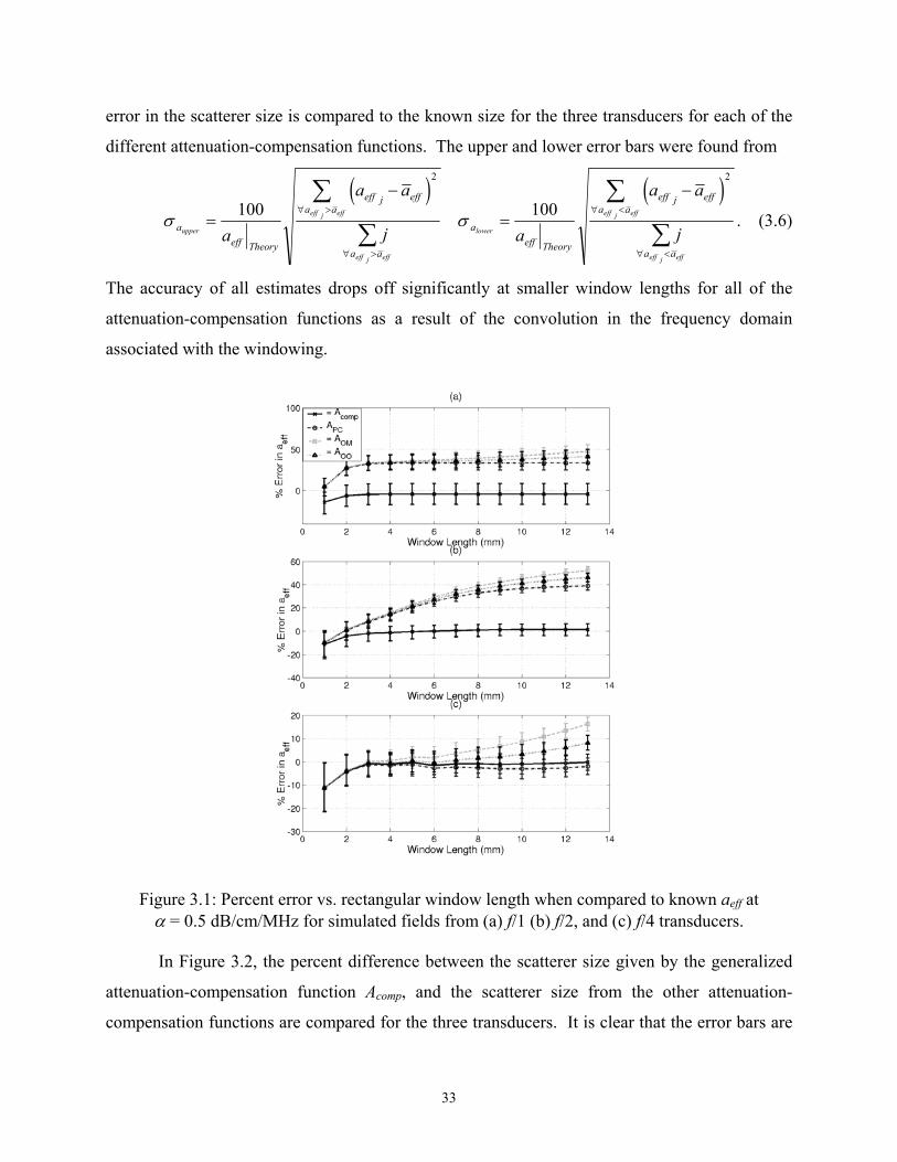
error in the scatterer size is compared to the known size for the three transducers for each of the
different attenuation-compensation functions. The upper and lower error bars were found from
σ σaeff Theory
eff j effa a
a a
aeff Theory
eff j effa a
a a
upper
eff j eff
eff j eff
lower
eff j eff
eff j eff
a
a a
j a
a a
j=
−
=
−∀ >
∀ >
∀ <
∀ <
∑
∑
∑
∑100 100
2 2
e j e j. (3.6)
The accuracy of all estimates drops off significantly at smaller window lengths for all of the
attenuation-compensation functions as a result of the convolution in the frequency domain
associated with the windowing.
Figure 3.1: Percent error vs. rectangular window length when compared to known aeff at α = 0.5 dB/cm/MHz for simulated fields from (a) f/1 (b) f/2, and (c) f/4 transducers.
In Figure 3.2, the percent difference between the scatterer size given by the generalized
attenuation-compensation function Acomp, and the scatterer size from the other attenuation-
compensation functions are compared for the three transducers. It is clear that the error bars are
33

reduced when the difference between the attenuation-compensation functions are found (Figure
3.2) as compared to plotting the straight error values (Figure 3.1). Hence, the differences
between the different attenuation-compensation functions should be relatively constant between
different scatterer distributions even though the absolute errors vary. Figure 3.3 shows the
percent differences again, but here the window length has been normalized with respect to the
calculated depth of field for the transducer (i.e., 7.08λof#2) [Kino, 1987], where λo was the
wavelength corresponding to the spectral peak from the reference spectrum (i.e., Vplane).
Figure 3.2: Percent difference vs. rectangular window length when compared to aeff found using Acomp in Equation (2.51) at α = 0.5 dB/cm/MHz for simulated fields from (a) f/1 (b) f/2, and (c)
f/4 transducers.
The errors (Figure 3.1) and differences (Figure 3.2) in AOM, AOO, and APC are larger for
the smaller f-number transducers (i.e., f/1 and f/2) and increase for longer window lengths. This
makes sense because the importance of diffraction along the beam axis increases with increasing
window length. Likewise, all four attenuation-compensation functions converge to the same
34

result for decreasing window lengths. Oelze and O’Brien [2002a] also observed this when
diffraction along the beam axis was neglected. Furthermore, Acomp yields excellent results
regardless of window length or f-number and even provides improved estimates for the scatterer
size for long window lengths when the beam is relatively unfocused (i.e., f/4). Also, when the
results for the f/1 and the f/2 transducers are compared, the errors/differences plateau with
increasing window length. Hence, the differences are greater for the f/1 transducer for smaller
window lengths and then are approximately the same for large window lengths.
Figure 3.3: Percent difference vs. window length normalized to the depth of focus (i.e. 7.08λof#2) when compared to aeff found using Acomp in Equation (2.51) at α = 0.5 dB/cm/MHz for simulated
fields from (a) f/1 (b) f/2, and (c) f/4 transducers.
The plateau can be better illustrated by the results for the normalized window lengths
(Figure 3.3). The plateau is reached once the window length is several times the calculated depth
of field; hence, the contributing scatterers are being limited by the focusing of the field and not
by the windowing. Also, when comparing the differences between the f/1 and the f/2 transducers
35
at the same normalized window length, the f/2 transducer has a larger difference for both the AOM
and AOO estimates, and the APC estimate values converge to the same difference of 37.6% for
normalized window lengths greater than approximately 2.5. Likewise, when comparing the
differences between the f/2 and the f/4 transducers at the same normalized window length, the f/4
transducer has a larger difference for the AOM estimate. Also, for the f/4 transducer, the
concavity of the APC estimate changed direction at a normalized window length of 0.65. Hence,
APC may overestimate the scatterer size for large enough window lengths. Therefore, the error in
using AOM is greater for transducers with larger f-number when comparing across the same
normalized window length, and the error in APC appears to plateau at sufficiently large
normalized window length at approximately 37.6%. However, the performance of the
attenuation-compensation functions cannot be generalized for small normalized window lengths
for the different focused transducers.
The improvement in the estimates using the new generalized attenuation-compensation
function can be illustrated further by considering the error in a (average size estimate) for
different values of attenuation at set rectangular window lengths of 6 and 13 mm (Figures 3.4
and 3.5, respectively). For the f/1 and f/2 transducers, A
eff
OM, AOO, and APC consistently
overestimate the scatterer size on the order of 20% to 100%, while Acomp gives almost exactly the
right answer with errors typically less than 2% with the largest error being 7.2%. However, for
the f/4 transducer, although AOM consistently overestimates the scatterer size, both AOO and APC
overestimate the scatterer size for small values of attenuation and then underestimate the
scatterer size as the attenuation is increased. This is in agreement with Oelze and O’Brien
[2002a] who also observed that AOM should overestimate the scatterer size and both AOO and APC
should underestimate the scatterer size for long window lengths when diffraction along the beam
axis can be neglected. The results for APC also agree with our predictions that APC will
under/overestimate the scatterer size based on the relative importance of α and wz. When
focusing dominates, APC overestimates the scatterer size, and when attenuation dominates, APC
underestimates the scatterer size. Once again, Acomp gives consistently good results for all
attenuation values for the f/4 transducer with errors less than 5%. Hence, including diffraction
along the beam axis with the generalized attenuation-compensation function improves the
accuracy of the scatterer size estimate and allows for more strongly focused sources (i.e., f/1 and
f/2) to be used in the data acquisition.
36
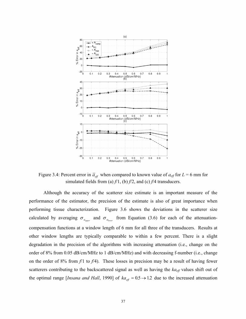
Figure 3.4: Percent error in a when compared to known value of aeff eff for L = 6 mm for
simulated fields from (a) f/1, (b) f/2, and (c) f/4 transducers. Although the accuracy of the scatterer size estimate is an important measure of the
performance of the estimator, the precision of the estimate is also of great importance when
performing tissue characterization. Figure 3.6 shows the deviations in the scatterer size
calculated by averaging σ aupper and σ alower
from Equation (3.6) for each of the attenuation-
compensation functions at a window length of 6 mm for all three of the transducers. Results at
other window lengths are typically comparable to within a few percent. There is a slight
degradation in the precision of the algorithms with increasing attenuation (i.e., change on the
order of 8% from 0.05 dB/cm/MHz to 1 dB/cm/MHz) and with decreasing f-number (i.e., change
on the order of 8% from f/1 to f/4). These losses in precision may be a result of having fewer
scatterers contributing to the backscattered signal as well as having the kaeff values shift out of
the optimal range [Insana and Hall, 1990] of kaeff = →05 12. . due to the increased attenuation
37

(i.e., from ka to kaeff = →0 67 16. . eff = →0 26 0 96. . ). More will be said on the effect of the kaeff
values in Chapter 7. Also, although the precision of the different attenuation-compensation
functions are comparable, Acomp is slightly less precise than the other algorithms for the f/1 and
f/2 transducers (i.e., change on the order of 1% to 7%). This loss in precision, however, is
insignificant compared to the simultaneous gain in accuracy.
eff
Figure 3.5: Percent error in a compared to known value of aeff for L = 13 mm for simulated
fields from (a) f/1, (b) f/2, and (c) f/4 transducers.
38
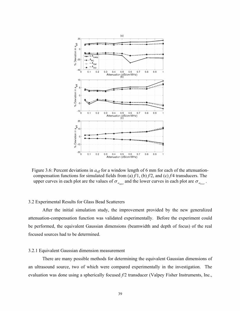
Figure 3.6: Percent deviations in aeff for a window length of 6 mm for each of the attenuation-compensation functions for simulated fields from (a) f/1, (b) f/2, and (c) f/4 transducers. The upper curves in each plot are the values of σ aupper
and the lower curves in each plot are σ alower.
3.2 Experimental Results for Glass Bead Scatterers
After the initial simulation study, the improvement provided by the new generalized
attenuation-compensation function was validated experimentally. Before the experiment could
be performed, the equivalent Gaussian dimensions (beamwidth and depth of focus) of the real
focused sources had to be determined.
3.2.1 Equivalent Gaussian dimension measurement
There are many possible methods for determining the equivalent Gaussian dimensions of
an ultrasound source, two of which were compared experimentally in the investigation. The
evaluation was done using a spherically focused f/2 transducer (Valpey Fisher Instruments, Inc.,
39
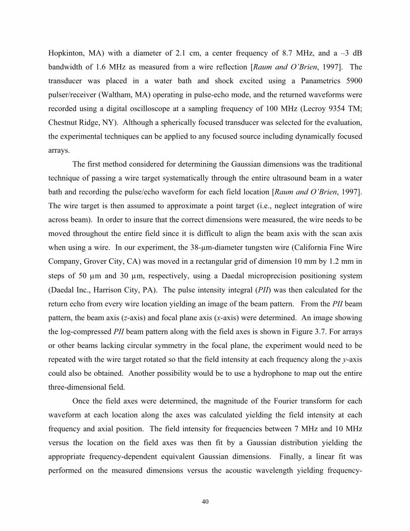
Hopkinton, MA) with a diameter of 2.1 cm, a center frequency of 8.7 MHz, and a –3 dB
bandwidth of 1.6 MHz as measured from a wire reflection [Raum and O’Brien, 1997]. The
transducer was placed in a water bath and shock excited using a Panametrics 5900
pulser/receiver (Waltham, MA) operating in pulse-echo mode, and the returned waveforms were
recorded using a digital oscilloscope at a sampling frequency of 100 MHz (Lecroy 9354 TM;
Chestnut Ridge, NY). Although a spherically focused transducer was selected for the evaluation,
the experimental techniques can be applied to any focused source including dynamically focused
arrays.
The first method considered for determining the Gaussian dimensions was the traditional
technique of passing a wire target systematically through the entire ultrasound beam in a water
bath and recording the pulse/echo waveform for each field location [Raum and O’Brien, 1997].
The wire target is then assumed to approximate a point target (i.e., neglect integration of wire
across beam). In order to insure that the correct dimensions were measured, the wire needs to be
moved throughout the entire field since it is difficult to align the beam axis with the scan axis
when using a wire. In our experiment, the 38-µm-diameter tungsten wire (California Fine Wire
Company, Grover City, CA) was moved in a rectangular grid of dimension 10 mm by 1.2 mm in
steps of 50 µm and 30 µm, respectively, using a Daedal microprecision positioning system
(Daedal Inc., Harrison City, PA). The pulse intensity integral (PII) was then calculated for the
return echo from every wire location yielding an image of the beam pattern. From the PII beam
pattern, the beam axis (z-axis) and focal plane axis (x-axis) were determined. An image showing
the log-compressed PII beam pattern along with the field axes is shown in Figure 3.7. For arrays
or other beams lacking circular symmetry in the focal plane, the experiment would need to be
repeated with the wire target rotated so that the field intensity at each frequency along the y-axis
could also be obtained. Another possibility would be to use a hydrophone to map out the entire
three-dimensional field.
Once the field axes were determined, the magnitude of the Fourier transform for each
waveform at each location along the axes was calculated yielding the field intensity at each
frequency and axial position. The field intensity for frequencies between 7 MHz and 10 MHz
versus the location on the field axes was then fit by a Gaussian distribution yielding the
appropriate frequency-dependent equivalent Gaussian dimensions. Finally, a linear fit was
performed on the measured dimensions versus the acoustic wavelength yielding frequency-
40
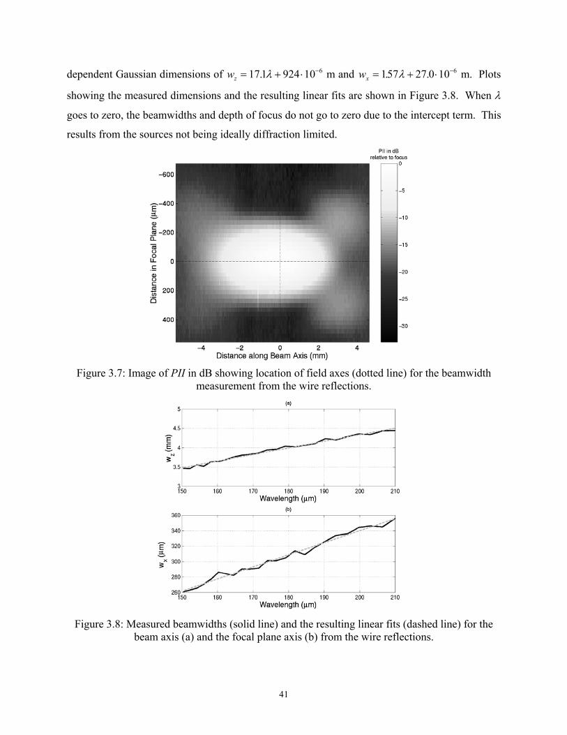
dependent Gaussian dimensions of wz = + ⋅ −171 924 10 6. λ m and wx = + ⋅ −157 27 0 10 6. .λ m. Plots
showing the measured dimensions and the resulting linear fits are shown in Figure 3.8. When λ
goes to zero, the beamwidths and depth of focus do not go to zero due to the intercept term. This
results from the sources not being ideally diffraction limited.
Figure 3.7: Image of PII in dB showing location of field axes (dotted line) for the beamwidth
measurement from the wire reflections.
Figure 3.8: Measured beamwidths (solid line) and the resulting linear fits (dashed line) for the
beam axis (a) and the focal plane axis (b) from the wire reflections.
41
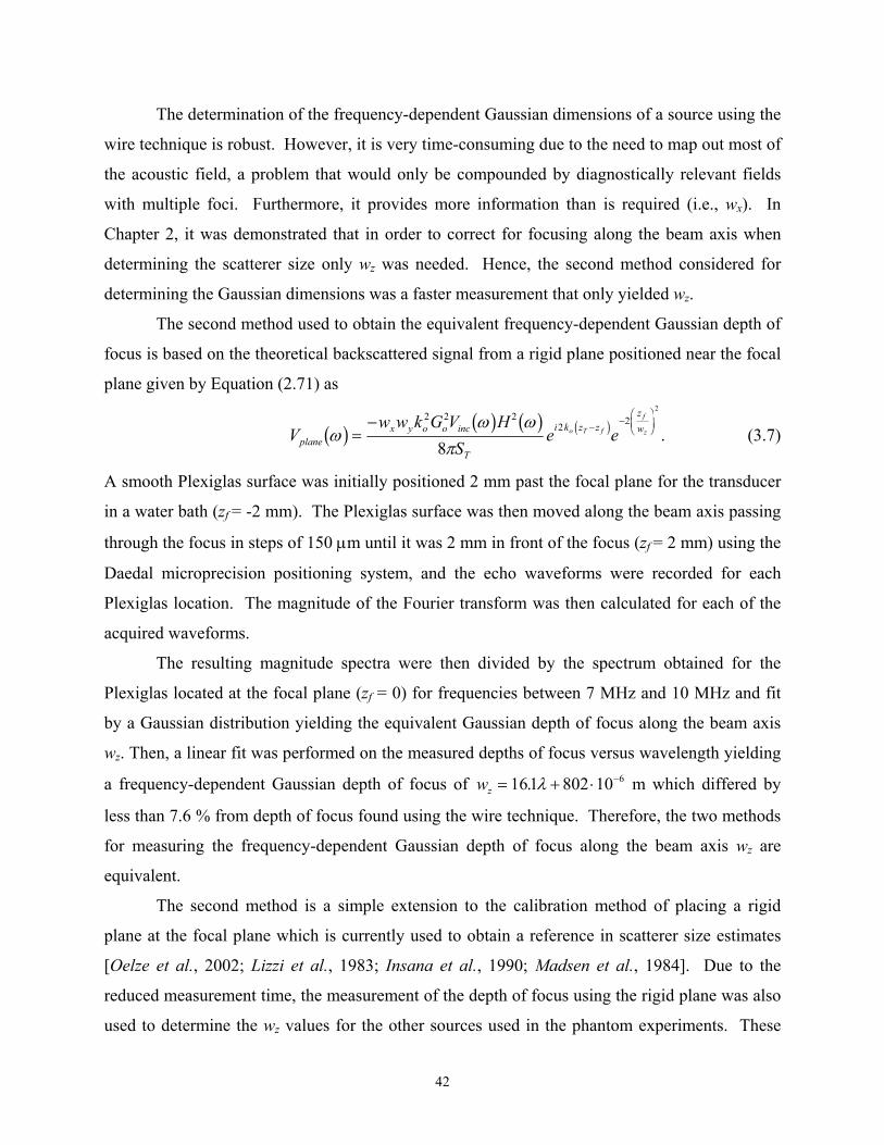
The determination of the frequency-dependent Gaussian dimensions of a source using the
wire technique is robust. However, it is very time-consuming due to the need to map out most of
the acoustic field, a problem that would only be compounded by diagnostically relevant fields
with multiple foci. Furthermore, it provides more information than is required (i.e., wx). In
Chapter 2, it was demonstrated that in order to correct for focusing along the beam axis when
determining the scatterer size only wz was needed. Hence, the second method considered for
determining the Gaussian dimensions was a faster measurement that only yielded wz.
The second method used to obtain the equivalent frequency-dependent Gaussian depth of
focus is based on the theoretical backscattered signal from a rigid plane positioned near the focal
plane given by Equation (2.71) as
Vw w k G V H
Se eplane
x y o o inc
T
i k z zzwo T f
f
zωω ω
πb g b g b g d i=
− −−FHGIKJ
2 2 22 2
8
2
. (3.7)
A smooth Plexiglas surface was initially positioned 2 mm past the focal plane for the transducer
in a water bath (zf = -2 mm). The Plexiglas surface was then moved along the beam axis passing
through the focus in steps of 150 µm until it was 2 mm in front of the focus (zf = 2 mm) using the
Daedal microprecision positioning system, and the echo waveforms were recorded for each
Plexiglas location. The magnitude of the Fourier transform was then calculated for each of the
acquired waveforms.
The resulting magnitude spectra were then divided by the spectrum obtained for the
Plexiglas located at the focal plane (zf = 0) for frequencies between 7 MHz and 10 MHz and fit
by a Gaussian distribution yielding the equivalent Gaussian depth of focus along the beam axis
wz. Then, a linear fit was performed on the measured depths of focus versus wavelength yielding
a frequency-dependent Gaussian depth of focus of wz = + ⋅ −161 802 10 6. λ m which differed by
less than 7.6 % from depth of focus found using the wire technique. Therefore, the two methods
for measuring the frequency-dependent Gaussian depth of focus along the beam axis wz are
equivalent.
The second method is a simple extension to the calibration method of placing a rigid
plane at the focal plane which is currently used to obtain a reference in scatterer size estimates
[Oelze et al., 2002; Lizzi et al., 1983; Insana et al., 1990; Madsen et al., 1984]. Due to the
reduced measurement time, the measurement of the depth of focus using the rigid plane was also
used to determine the wz values for the other sources used in the phantom experiments. These
42
values are provided in Table 3.1 along with the scan length the planar reflector was moved when
acquiring the reflections. Variations in the scan length did not significantly change the resulting
wz values indicating secondary field properties (i.e., waveform curvature) did not dramatically
effect the measured Gaussian depth of focus for the focal region.
Table 3.1: Relevant properties of transducers used in the phantom experiments.
f# Center Frequency
-3 dB Bandwidth
TransducerDiameter
Scan Length (Step Size) to
find wz wz
Depth into
Phantom
1 8.7 MHz 1.5 MHz 2.1 cm -2 mm 2 mm (50 µm) 3.22λ + 1285 µm 6 mm
2 8.7 MHz 1.6 MHz 2.1 cm -2 mm 2 mm (150 µm) 16.1λ + 802 µm 12.5 mm
4 9.4 MHz 3.8 MHz 1.4 cm -8 mm 8 mm (200 µm) 76.8λ + 4207 µm 15 mm
3.2.2 Experimental procedure and results
The phantom experiments were designed to validate the use of focused sources in
predicting scatterer size as well as investigate the effects of focusing along the beam axis in
greater detail. Hence, the three transducers described in Table 3.1 were used to estimate the
radius of glass beads in a tissue mimicking phantom. The reported center frequencies and –3 dB
bandwidths had been previously measured by a wire reflection technique [Raum and O’Brien,
1997].
The agar phantom used in the experiment was produced at the University of Wisconsin
and was part of an interlaboratory comparison of ultrasonic backscatter, attenuation, and sound
speed measurements [Madsen et al., 1999]. The phantom consisted of degassed water, agar, n-
proponal, finely powdered graphite, and glass beads whose radii varied between 22.5 µm and
26.5 µm with an average concentration of 20.454 /mm3. The attenuation of the phantom (0.55 ±
0.08 dB/cm/MHz) was measured by both insertion loss techniques as well as by observing the
change in backscatter with propagation depth into the phantom at room temperature. The sound
speed of the phantom was reported by Madsen et al. [1999] to have a mean value of 1534.4 m/s
at 22 oC with a temperature dependence of 1.7 m/s/ oC.
The experiments were performed by first positioning a rigid plane at the focus of the
transducer in a degassed water bath. The transducers were shock excited using a Panametrics
43
5900 pulser/receiver operating in pulse-echo mode, and the echo waveforms were captured using
a Lecroy 9354 TM digital oscilloscope with a sampling frequency of 100 MHz. The focus was
defined as the plane location that resulted in the largest peak-peak voltage for the returned echo
waveform. This echo waveform was then recorded as the reference waveform Vplane. The rigid
plane used to obtain the reference waveform was made of either Plexiglas or polished metal.
The plane was then moved along the beam axis so that the values of wz could be determined as
described previously.
The phantom was then placed such that the reflection from the front surface of the
phantom corresponded in time with the previously acquired reference waveform, thereby
positioning the front surface of the phantom in the focal plane of the transducer. The focus was
then moved into the phantom a known distance by using the Daedal microprecision positioning
system. Care was taken so that secondary reflections between the surface of the transducer and
the surface of the phantom did not interfere with the speckle from the glass beads. The distance
the focus was moved into the phantom for each transducer is also given in Table 3.1.
After positioning the focus, 25 independent RF echoes were acquired by moving the
phantom along a square grid parallel to the focal plane using the Daedal microprecision
positioning system. The grid consisted of 5 columns and 5 rows each separated by a distance of
450 µm, 450 µm, and 1 mm for the f/1, f/2, and f/4 transducers, respectively. For each grid
position, the echo waveform was averaged between 1000 to 2200 times to remove as much
electronic noise as possible.
During processing, each RF echo was windowed by a rectangular gating function
centered at the focus, the location of which was known from the reference signal. A rectangular
gating function was selected because the traditional attenuation compensation functions (AOO and
AOM) are defined for a rectangular gate. The positioning was done by measuring the water
temperature, calculating the sound speed of the water/phantom medium (co and c) from the
temperature, and then using these sound speeds to position the window at the correct location in
time. The length of the gating functions varied from 1 mm to 13 mm in steps of 0.5 mm with
corresponding time gates given by T L cwin = 2 . After windowing, the magnitude of the Fourier
transforms for each RF echo were averaged together yielding an estimate for E . An
estimate for the radius of the glass beads was then obtained by finding the value of a
Vrefl ωb g 2
eff that
44
minimized the average squared difference (ASD) given by Equation (2.75). The minimization
was done for frequencies in the range of 6.5 MHz to 10.5 MHz for all three of the transducers so
that differences in the bandwidth of the transducers would not affect the comparison.
The average value of the glass bead radius for window lengths between 3 mm and 8 mm
found using the generalized attenuation compensation function was 26.1 µm, 22.8 µm, and 22.9
µm for the f/1, f/2, and f/4 transducers, respectively. Hence, the estimated bead radii were well
within the range of bead radii known to be in the phantom (i.e., 22.5 µm to 26.5 µm).
Previously, it was shown that the differences between the different attenuation-compensation
functions should be relatively constant between different scatterer distributions even though the
absolute errors would vary. Hence, the percent difference between the traditional attenuation-
compensation functions and the generalized attenuation-compensation function relative to the
mean glass bead radius of 24.5 µm was used in this evaluation.
The percent difference versus window length for each of the transducers is shown in
Figure 3.9, and the percent difference versus normalized window length where the window
length has been divided by the calculated depth of field for the transducer (i.e., 7.08λof#2) is
given in Figure 3.10. The traditional attenuation-compensation functions APC, AOM, and AOO all
predict larger bead sizes than the generalized attenuation-compensation function for the f/1 and
f/2 transducers. Also, for the f/4 transducer, APC gives a smaller estimate while AOM and AOO
continue to give larger estimates. This same qualitative behavior was also observed in our earlier
simulation study. However, there was not quantitative agreement in the amount of improvement
provided by the new generalized attenuation-compensation function.
For the Gaussian scatterers, the generalized attenuation-compensation function gave an
improvement in the scatterer size estimate of 40% to 50% over the traditional attenuation-
compensation functions for the f/2 transducer with a window length of 13 mm and an attenuation
of 0.5 dB/cm/MHz. In the experiment, the f/2 transducer only gave an improvement of 12% to
18%. Likewise, the improvement in the experiment for the f/1 transducer was only about 3.5%
to 6% when our previous simulation study with Gaussian scatterers predicted an improvement of
35% to 55%. Theoretically, the experimental difference should have been larger due to the
slightly increased attenuation. Also, in the experiments, the f/1 transducer yielded improvements
in the scatterer size estimate much smaller than the f/2 transducer when our previous simulation
study seemed to indicate that the differences should plateau at approximately the same values as
45

the window length is increased for both transducers. Even the f/4 transducer had less
improvement in the experiment (i.e., 7.1% for AOM at 13 mm) as compared to the simulation
study (i.e., 17% for AOM at 13 mm). Clearly, these differences in the improvements in the
scatterer size estimate when using Acomp in the experiment as compared to the earlier simulations
with Gaussian scatterers need to be understood.
Figure 3.9: Experimental results for percent difference in aeff versus window length found using traditional attenuation compensation functions as compared to aeff found using Acomp for a glass
bead phantom with an attenuation of 0.55 ± 0.08 dB/cm/MHz, a concentration of 20.454 beads/mm3, and a mean bead radius of 24.5 µm from spherically focused transducers with f-
numbers of (a) f/1, (b) f/2, and (c) f/4.
46
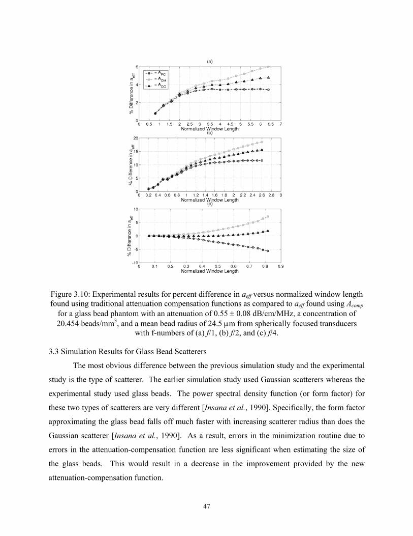
Figure 3.10: Experimental results for percent difference in aeff versus normalized window length found using traditional attenuation compensation functions as compared to aeff found using Acomp
for a glass bead phantom with an attenuation of 0.55 ± 0.08 dB/cm/MHz, a concentration of 20.454 beads/mm3, and a mean bead radius of 24.5 µm from spherically focused transducers
with f-numbers of (a) f/1, (b) f/2, and (c) f/4. 3.3 Simulation Results for Glass Bead Scatterers
The most obvious difference between the previous simulation study and the experimental
study is the type of scatterer. The earlier simulation study used Gaussian scatterers whereas the
experimental study used glass beads. The power spectral density function (or form factor) for
these two types of scatterers are very different [Insana et al., 1990]. Specifically, the form factor
approximating the glass bead falls off much faster with increasing scatterer radius than does the
Gaussian scatterer [Insana et al., 1990]. As a result, errors in the minimization routine due to
errors in the attenuation-compensation function are less significant when estimating the size of
the glass beads. This would result in a decrease in the improvement provided by the new
attenuation-compensation function.
47
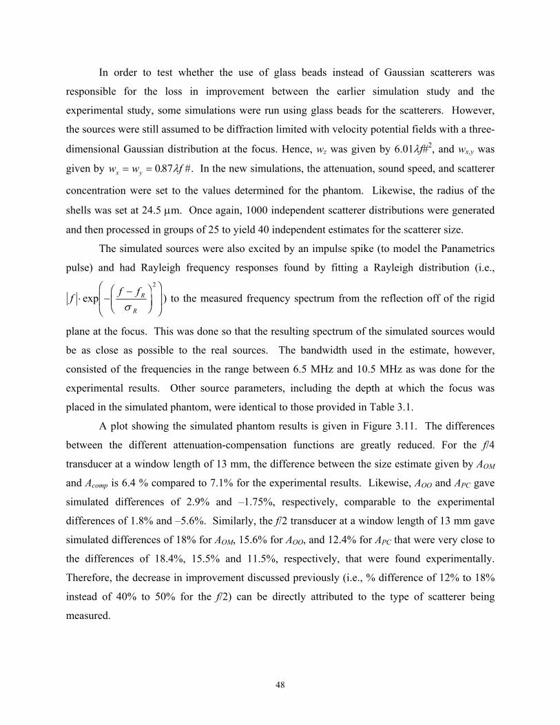
In order to test whether the use of glass beads instead of Gaussian scatterers was
responsible for the loss in improvement between the earlier simulation study and the
experimental study, some simulations were run using glass beads for the scatterers. However,
the sources were still assumed to be diffraction limited with velocity potential fields with a three-
dimensional Gaussian distribution at the focus. Hence, wz was given by 6.01λf#2, and wx,y was
given by w w fx y= = 087. #λ . In the new simulations, the attenuation, sound speed, and scatterer
concentration were set to the values determined for the phantom. Likewise, the radius of the
shells was set at 24.5 µm. Once again, 1000 independent scatterer distributions were generated
and then processed in groups of 25 to yield 40 independent estimates for the scatterer size.
The simulated sources were also excited by an impulse spike (to model the Panametrics
pulse) and had Rayleigh frequency responses found by fitting a Rayleigh distribution (i.e.,
f f f R
R
⋅ −−FHG
IKJ
FHG
IKJ
expσ
2
) to the measured frequency spectrum from the reflection off of the rigid
plane at the focus. This was done so that the resulting spectrum of the simulated sources would
be as close as possible to the real sources. The bandwidth used in the estimate, however,
consisted of the frequencies in the range between 6.5 MHz and 10.5 MHz as was done for the
experimental results. Other source parameters, including the depth at which the focus was
placed in the simulated phantom, were identical to those provided in Table 3.1.
A plot showing the simulated phantom results is given in Figure 3.11. The differences
between the different attenuation-compensation functions are greatly reduced. For the f/4
transducer at a window length of 13 mm, the difference between the size estimate given by AOM
and Acomp is 6.4 % compared to 7.1% for the experimental results. Likewise, AOO and APC gave
simulated differences of 2.9% and –1.75%, respectively, comparable to the experimental
differences of 1.8% and –5.6%. Similarly, the f/2 transducer at a window length of 13 mm gave
simulated differences of 18% for AOM, 15.6% for AOO, and 12.4% for APC that were very close to
the differences of 18.4%, 15.5% and 11.5%, respectively, that were found experimentally.
Therefore, the decrease in improvement discussed previously (i.e., % difference of 12% to 18%
instead of 40% to 50% for the f/2) can be directly attributed to the type of scatterer being
measured.
48
Figure 3.11: Simulation results for percent difference in aeff found using traditional attenuation compensation functions as compared to aeff found using Acomp for a glass bead phantom with an
attenuation of 0.55 ± 0.08 dB/cm/MHz, a concentration of 20.454 beads/mm3, and bead radius of 24.5 µm from spherically focused transducers with f-numbers of (a) f/1, (b) f/2, and (c) f/4, and
wz = 6.01λf#2.
The influence of scatterer type on the improvement provided by the generalized
attenuation-compensation function is of great importance for estimating scatterer sizes of
biological tissue because the fundamental scatterer geometry (type) in tissue has not been
determined. Hence, the improvement of the new generalized attenuation-compensation function
compared to the traditional attenuation-compensation functions may be even more significant in
a clinical setting because the correct scatterer geometry may exhibit an even stronger dependence
on the attenuation-compensation function.
Although the type of scatterer and the subsequent dependence on the attenuation-
compensation function explains the reduction in the improvement provided by the new
attenuation-compensation function, it does not explain why the plateau of the f/1 transducer (i.e.,
49
difference for APC of 3.4 %) was different than the plateau for the f/2 transducer (i.e., difference
for APC of 11.5 %). Both of the previous simulation studies showed them converging to the same
value whereas in the experiment they converged to different amounts of improvement. In order
to understand this behavior, another difference between the Gaussian simulation study and the
experimental study was explored, namely the wavelength dependence of the effective Gaussian
beamwidth along the beam axis, wz. In the earlier simulations, wz was directly proportional to the
wavelength (i.e., ), but in the experiment, ww fz = 6 01 2. #b g λ⋅ z had the form
w w wz zm zb= ⋅ +λ (3.8)
where wzb was a constant independent of wavelength (Table 3.1).
In order to understand the impact of the wavelength dependence of wz, the curves of
ln A Acomp OMd i and ln versus frequency were fit by a line. The slope of this line
could then be used to predict how the scatterer size estimate from A
A Acomp PCd
0
mµ
01 1812. #fb g b⋅
icomp would compare to the
estimate from AOM and APC. A positive slope means that the estimate from APC/OM is larger than
the estimate obtained from Acomp. Likewise, a negative slope means that the estimate from
APC/OM is smaller than the estimate from Acomp. The wavelength dependence of wz was evaluated
for three different wz values: (a) 6 , as was used in the previous simulation studies, (b)
, similar to the wavelength dependence found for the measured
transducers, and (c) 6 . The calculations were performed for window lengths
normalized to the traditional depth of focus (i.e., 7.08λ
1 2. #fb g ⋅λ
mgµ
6 01 12852. #fb g ⋅ +λ
of#2) of 0.5, 1, and 2.5 as well as for a
window length of 8 mm. The resulting slopes are shown in Figures 3.12 and 3.13.
Consider first the wz values of 6 shown by the solid curves. For any given
normalized window length, the A
01 2. #fb g ⋅λOM estimate is larger than the Acomp estimate and increases with
increasing f-number. Likewise, the APC estimate is larger than the Acomp estimate for smaller f-
numbers and then decreases with increasing f-number for smaller normalized window lengths
resulting in the APC estimate being smaller than the Acomp estimate. For larger normalized
window lengths, the APC estimate is always larger than the Acomp estimate and there is no longer
any dependency on f-number corresponding to the plateau observed earlier.
50
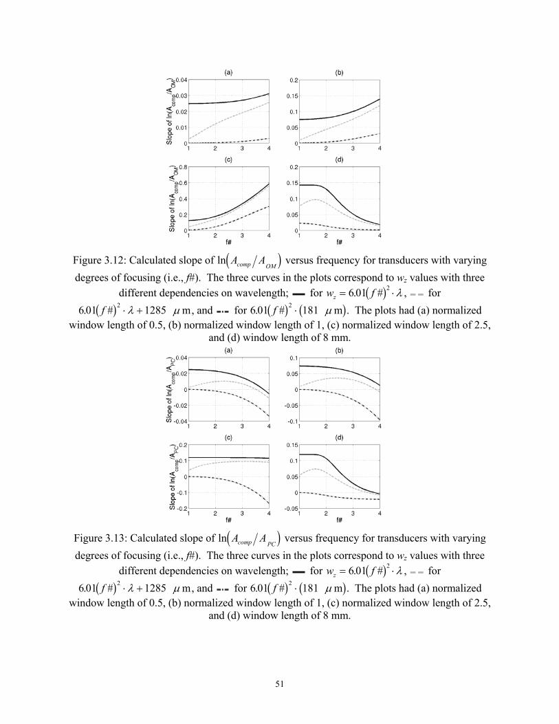
Figure 3.12: Calculated slope of ln versus frequency for transducers with varying degrees of focusing (i.e., f#). The three curves in the plots correspond to w
A Acomp OMd iz values with three
different dependencies on wavelength; for w f , z = 6 01 2. #b g λ⋅ for , and 6 01 12852. #fb g ⋅ +λ µm for 6 . The plots had (a) normalized
window length of 0.5, (b) normalized window length of 1, (c) normalized window length of 2.5, and (d) window length of 8 mm.
01 1812. #fb g b⋅ mgµ
Figure 3.13: Calculated slope of ln versus frequency for transducers with varying degrees of focusing (i.e., f#). The three curves in the plots correspond to w
A Acomp PCd iz values with three
different dependencies on wavelength; for w f , z = 6 01 2. #b g λ⋅ for , and 6 01 12852. #fb g ⋅ +λ µm for 6 . The plots had (a) normalized
window length of 0.5, (b) normalized window length of 1, (c) normalized window length of 2.5, and (d) window length of 8 mm.
01 1812. #fb g b⋅ mgµ
51
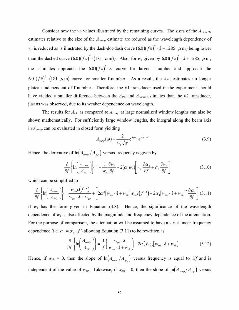
Consider now the wz values illustrated by the remaining curves. The sizes of the APC/OM
estimates relative to the size of the Acomp estimate are reduced as the wavelength dependency of
wz is reduced as is illustrated by the dash-dot-dash curve (6 ) being lower
than the dashed curve (6 ). Also, for w
01 12852. #fb g ⋅ +λ
01 2. #fb gmµ
m m
mg
01 1812. #fb g b g⋅ µ
1 2. #fb g ⋅λz given by 6 ,
the estimates approach the 6 0 curve for larger f-number and approach the
curve for smaller f-number. As a result, the A
1285⋅ +λ µ
6 01 1812. #fb g b⋅ µ PC estimates no longer
plateau independent of f-number. Therefore, the f/1 transducer used in the experiment should
have yielded a smaller difference between the APC and Acomp estimates than the f/2 transducer,
just as was observed, due to its weaker dependence on wavelength.
The results for APC as compared to Acomp at large normalized window lengths can also be
shown mathematically. For sufficiently large window lengths, the integral along the beam axis
in Acomp can be evaluated in closed form yielding
Aw
ecompz
zTωπ
α αb g = −2 4 12 2
e wz . (3.9)
Hence, the derivative of ln versus frequency is given by A Acomp PCd i∂∂FHGIKJ
RSTUVW= −
∂∂
−∂∂
+∂∂
LNM
OQPf
AA w
wf
w wf
wf
comp
PC z
zz z
zln 1 2 11
1α α αb g (3.10)
which can be simplified to
∂∂FHGIKJ
RSTUVW=
⋅ ++ ⋅ + − ⋅ +
∂∂
LNM
OQP
−−
fAA
w c fw w
w w w c f w wf
comp
PC
zm
zm zbzm zb zm zm zbln
2
12 2
12 12 2
c h c hλ
α λ α λ α (3.11)
if wz has the form given in Equation (3.8). Hence, the significance of the wavelength
dependence of wz is also affected by the magnitude and frequency dependence of the attenuation.
For the purpose of comparison, the attenuation will be assumed to have a strict linear frequency
dependence (i.e. α α1 = ⋅o f ) allowing Equation (3.11) to be rewritten as
∂∂FHGIKJ
RSTUVW=
⋅⋅ +
FHG
IKJ − ⋅
fAA f
ww w
fw w wcomp
PC
zm
zm zbo zb zm zbln 1 2 2λ
λα λ + . (3.12)
Hence, if wzb = 0, then the slope of ln versus frequency is equal to 1/f and is
independent of the value of w
A Acomp PCd izm. Likewise, if wzm = 0, then the slope of ln versus A Acomp PCd i
52

frequency decreases approximately parabolically with increasing values of wzb. Both of these
effects are evident in Figure 3.13c.
The impact of the wavelength dependence of wz on the different attenuation-
compensation functions was further tested by repeating the simulation of the glass bead
phantoms using the wz values found experimentally. Once again, the attenuation, sound speed,
and scatterer concentration were set to the values determined for the phantom, and the radius of
the shells was set at 24.5 µm. Also, 40 independent estimates were obtained for 1000
independent scatterer distributions that were generated and then processed in groups of 25 using
frequencies in the range between 6.5 MHz and 10.5 MHz. The simulated sources were also
modeled to have the same Rayleigh frequency response as was found experimentally and were
excited by an impulse spike. The resulting differences between the different attenuation-
compensation functions are shown in Figure 3.14. Once the measured values for wz were used in
the simulations, the differences between the attenuation-compensation functions for the f/1
transducer at 8 mm were 7.4%, 5.9%, and 4.3% whereas the differences for the f/2 transducer at
13 mm were 16%, 13.4%, and 10% for AOM, AOO, and APC, respectively. Hence, APC for the f/1
transducer and the f/2 transducer now plateau at different levels in agreement with the observed
experimental results. Therefore, the wavelength dependence of wz was responsible for their
earlier discrepancy. Furthermore, the differences found experimentally and the mean differences
found in the simulations using the correct value for wz were consistently within 2.5% of each
other, validating the theoretical analysis provided in Chapter 2.
3.4 Chapter Summary
In this chapter, the use of focused sources for estimating scatterer sizes was investigated
through simulation studies and phantom experiments. First, simulation studies with Gaussian
scatterers demonstrated that including the effects of diffraction along the beam axis improves the
accuracy of the scatterer size estimator even for a weakly focused f/4 transducer. The
improvement in accuracy for the more strongly f/1 and f/2 transducers was on the order of 20%
to 100% depending on the length of the window and the amount of attenuation.
53
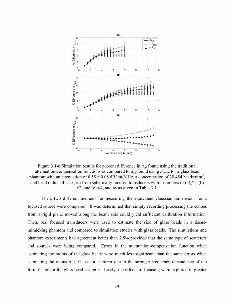
Figure 3.14: Simulation results for percent difference in aeff found using the traditional
attenuation-compensation functions as compared to aeff found using Acomp for a glass bead phantom with an attenuation of 0.55 ± 0.08 dB/cm/MHz, a concentration of 20.454 beads/mm3, and bead radius of 24.5 µm from spherically focused transducers with f-numbers of (a) f/1, (b)
f/2, and (c) f/4, and wz as given in Table 3.1.
Then, two different methods for measuring the equivalent Gaussian dimensions for a
focused source were compared. It was determined that simply recording/processing the echoes
from a rigid plane moved along the beam axis could yield sufficient calibration information.
Then, real focused transducers were used to estimate the size of glass beads in a tissue-
mimicking phantom and compared to simulation studies with glass beads. The simulations and
phantom experiments had agreement better than 2.5% provided that the same type of scatterers
and sources were being compared. Errors in the attenuation-compensation function when
estimating the radius of the glass beads were much less significant than the same errors when
estimating the radius of a Gaussian scatterer due to the stronger frequency dependence of the
form factor for the glass bead scatterer. Lastly, the effects of focusing were explored in greater
54

55
detail, and it was found that the improvement provided by the new generalized attenuation-
compensation function decreased as the wavelength dependence of wz was reduced.
Before concluding, recall that the theoretical derivations in Chapter 2 neglected multiple
scattering. This is the traditional approximation made when performing this type of analysis
[Insana et al., 1990] due to the weak scattering and large attenuation of biological tissue. The
good agreement between the real phantom experiments and computer simulations demonstrate
that multiple scattering is not important for this application and need not be considered in the
remaining simulations provided in this thesis.
CHAPTER 4
GAUSSIAN TRANSFORMATION ALGORITHM
As discussed in Chapter 2, estimating the scatterer size from the statistics of the
backscattered signal can only yield accurate results when the attenuation of the tissue medium is
properly compensated. However, in real tissues, the attenuation is not known a priori. Hence,
the algorithms presented in the following chapters endeavored to determine the attenuation so
that the scatterer size might be estimated more accurately. The first algorithm, presented in this
chapter, attempted to find the scatterer size and attenuation from two separate effects on the
backscattered spectrum. The algorithm assumed that the backscattered signal has a Gaussian
spectrum where the scatterer size and total attenuation are independent Gaussian transformations.
The analysis is similar to that presented by Wear [2002] who uses Gaussian transformations to
predict the backscattered spectrum for given scatterers and attenuation.
4.1 Background Theory
In Chapter 2, the expected backscattered voltage E V from a tissue region was given
by
refl
2
E V , (4.1) k VF aArefl o plane
eff
comp
2 4 2∝ ω
ω
ωγb g d ib g
,
where Vplane ωb g is the Fourier transform of the voltage signal returned from the transducer when
the acoustic signal is reflected from a rigid plane placed at the focal plane, is a form
factor related to the scatterer geometry and size a
F aeffγ ω ,d ieff, and Acomp is the attenuation-compensation
function given by
56

A e
ds g s e ecomp
z
z win z
sw s
L
L
T
z
z z
= FHGG
IKJJ
−
−z
4
44
2
22
21
α
αb g/
/. (4.2).
For weakly focused transducers and “small” window lengths the integral term in Equation (4.2)
can be ignored. Also, if we assume that the attenuation along the propagation path has a linear
dependence on frequency, Acomp can be approximated as e z fT o4 α . Furthermore, if the form factor
can be expressed as a power law e , at least over a limited frequency range, and
the source/diffraction characteristics can be assumed Gaussian (i.e.,
F aeffγ ω ,d i Af n−
k Vo plane4 ωb g f fo2
2
22σω
b g∝ −
−FHG
IKJexp ), then the backscattered voltage is given by [Wear, 2002]
E e e eVrefl
f f
Af z fo
nT o
2 2 4
2
2
∝−
−
− −
b gσ αω . (4.3)
Equation (4.3) can also be approximated as a Gaussian by making the following
simplifications:
E Vf f
Af z f
f fA f n f f f
n n f f fz f
f fz Anf f
An n f f f
f f
reflo n
T o
oon
o on o o
n
T o
oT o o
n o on
o
22
2
2
21
2 2
2
21
2 2
2
24
21
24
24
12
∝ −−
− −FHG
IKJ
∝ −−
− + − +− −
+FHG
IKJ−
FHGG
IKJJ
∝ −−
− + −− −
+FHG
IKJ
∝ −−
−−
−−
exp
exp ...
exp ( ) ...
exp
b g
b g b g b gb g
b g b gb g
b g
σα
σα
σα
ω
ω
ω
21 1 42
2 1
σα
ω
+ −LNM
OQP− + +
FHG
IKJ
− −An n f z Anf fon
T o onb g ( ) ...
∝ −− +
− + +FHG
IKJ
∝ −− − +
− +FHG
IKJ
−
−
exp ~ ( ) ..
exp~
~ ( ) .
f ff fz Anf f
f f Anf f fz f
o oT o o
n
o on
oT o
2 2
21
2 2 1 2
2
22
4
2
24
σα
σ
σα
ω
ω
ω
c h
.
..
∝ −−
− +F
HGG
I
KJJexp
~
~ ( ) ...f f
z fo
T o
d i222
4σ
αω
57
∝ −− − +
+FHGG
IKJJexp
~ ~ ~
~ ...f f z f fo T o o
2 2
2
2 4
2
α σ
σω
ω
d i 2
∝ −− ′
+F
HGG
I
KJJexp
~
~ ...f f od i2
22σ ω
,
(4.4)
where ~ ~
~
~ ~ ~ .
f f Anf
An n f
f f z
o o on
on
o o T o
= −
= + −LNM
OQP
′ = −
−
−
−
σ
σσ
α σ
ω
ωω
ω
2 1
22
21
2
1 1
4
b g (4.5)
Hence, to a first-order approximation, the scatterer size changes the bandwidth and center
frequency of the returned spectrum whereas the total attenuation along the propagation path,
after correcting for scatterer size, only affects the center frequency. Therefore, in the first
algorithm, the scatterer size was found by analyzing the Gaussian bandwidth of the scattered
signal. Once the size was known, the total attenuation could be found by correcting for the
scatterer size and then analyzing the down shift in the center frequency.
4.2 Determine Bandwidth and Center Frequency
In order to find the scatterer size, the scattered spectrum had to be fit with a Gaussian
spectrum in order to determine the appropriate bandwidth and center frequency. However, the
fitting was complicated by the spectral fluctuations introduced by the random scatterer spacing.
To improve the fitting, 25 independent backscattered spectra from the same “tissue” region were
averaged in the log domain, that is,
E V f P f Vrefl scat jj
b g b g e j2 2
1
25125
≅ =FHG
IKJ=
∑exp ln . (4.6)
The averaging was done in the log domain because it was assumed that the transmitted pulse is
convoluted with the random medium to generate the reflected spectrum. Hence, the noise
resulting from the random scatterer spacing should be included as a multiplicative random
impulse train in the frequency domain. Multiplicative noise is most effectively removed by
averaging in the log domain. The impact of averaging the signals in the log domain as opposed to
58
the normal frequency domain will be analyzed in Chapter 5. After averaging, the resulting
spectrum was fit to a Gaussian spectrum, also in the log domain, to yield the center frequency ~′f
and bandwidth σ , given by
o
~ω2
~ , ~ min mean , ~ , ~~
~
′ = − ′ −FH IKRST
UVW∀ ′∀
f P f P f fo f n p o no
σ σω
σ
ω
ω
2 22
2
b g d ie jP , (4.7)
where
P fP f
P f
P f ff f
P P f P f f
nscat
f scat
p oo
n n p o
b g b gb gc h
d i d i
b g d ie j
=FHGG
IKJJ
′ = −− ′
= − ′
∀
lnmax
, ~ , ~~
~
mean , ~ , ~ .
σσ
σ
ωω
ω
2
2
2
2
2 (4.8)
By doing the fit in the log domain and subtracting P , the effect of any multiplicative constants
was removed. n
Another key issue when fitting the scattered spectrum is the selection of the frequency
range over which to perform the fit. This is especially true in the presence of electronic noise.
Using more frequencies increases the accuracy of the final result provided that frequencies close
to the noise floor of the system are not included. Hence, the fit used all frequencies
corresponding to signal values satisfying
10 30 10logmax
max mean logmax
P fP f
P fP f
scat
f scat polynomialfit
scat
f scat polynomialfit
b gb gc h
b gb gc h
∀ ∀
FHGG
IKJJ
RS|T|
UV|W|
> −FHGG
IKJJ
RS|T|
UV|W|
F
H
GGGG
I
K
JJJJ
L
N
MMMM
O
Q
PPPP
F
H
GGGG
I
K
JJJJ (4.9)
where the spectra was fit by a polynomial of large degree (i.e., 50) to reduce the impact of
spectral variations on the selected frequency range. More will be said about this method for
selecting the frequency range in Chapter 5.
In order to find the change in bandwidth and center frequency resulting from scatterer
size and total attenuation, the scattered spectrum needs to be compared to a reference spectrum.
Hence, the signal returned from a rigid plane placed at the focal plane of the transducer was used
as a reference. The spectrum from the plane was multiplied by k and fit by a Gaussian
distribution to get the original bandwidth σ
o4
ω and center frequency fo. Because the spectrum was
59
not corrupted by the orientation of random scatterers, the best fits were obtained by fitting in the
normal frequency domain and not in the log domain by solving
fk V
k V
f fo f
o plane
f o plane
o
o, min mean
maxexpσ
ω
ω σω
σ ωω
24 2
4 2
2
2
2
22
=F
HGGG
I
KJJJ− −
−FHG
IKJ
F
HGGG
I
KJJJ
F
H
GGG
I
K
JJJ
RS||
T||
UV||
W||
∀∀ ∀
b gb g
b g . (4.10)
4.3 Algorithm to Find Scatterer Size and Total Attenuation
Now that the methods for finding the bandwidth and center frequency for both the
scattered and reference signals have been discussed, the algorithms used to find the scatterer size
and total attenuation can be explained. First, the bandwidth for the scattered signal ~σω2 was
found as discussed previously. Then the reference signal k V was multiplied by the
appropriate form factor F and fit by a Gaussian in the normal frequency domain to
determine the adjusted bandwidth. The value of a
o plane4 2
ωb gaeffγ ω ,d i
eff was then varied to minimize the difference
between the bandwidth of the scattered signal and the adjusted reference signal using a standard
minimization routine in Matlab.
Before proceeding, several important features of the algorithm need to be highlighted.
First, aeff was solved by minimization rather than directly by an equation of the form
A an n feff
ond i b g=
−−
LNM
OQP−
11
1 12 2 2~σ σω ω
(4.11)
which can be derived from Equation (4.5). Although using Equation (4.11) can yield correct
results, preliminary simulations and phantom experiments showed that it lacked the precision of
the minimization routine and hence was not considered further in the analysis. Another
important feature of the algorithm was that all of the spectral adjustments (i.e., multiplying by
the hypothesized form factor) were done on the reference spectrum rather than on the scattered
spectrum. This was done so that the algorithm would not amplify any electronic noise in the
scattered signal.
Once the scatterer size was known, the total attenuation could be found by multiplying
the reference spectrum by the correct form factor and fitting the result to a Gaussian spectrum to
60
determine the adjusted center frequency ~fo . The center frequency ~′fo and bandwidth ~σω2 for the
scattered spectrum found previously could then be used to find the total attenuation according to
zf f
T oo o
ασ ω
=− ′~ ~
~d i
4 2 . (4.12)
A minimization routine was also attempted for finding the total attenuation, but had no
advantage over solving the equation directly.
4.3.1 Compensating for Electronic Noise
In addition to solving for the attenuation and scatterer size independently, a method to
compensate for the effects of electronic noise was developed. Assume that the electronic noise is
additive, white, and with zero mean. Then, the expected spectrum over the set of possible
additive noise for a given scatterer distribution is given by
E V f N f V f EN f
V fV f
E N f
V fN refl refl N
reflrefl
N
refl
b g b g b g b gb g b g
b gb g
+ = +LNMM
OQPP = +
F
HGG
I
KJJ
2 22
2
2
21 1 , (4.13)
where N(f) is the additive electronic noise and EN[~] is the expected value with respect to the
noise statistics. Hence, the averaging of the spectra in the log domain results in a corrupted
spectrum given by
P f V fE N f
V f
V fE N f
V f
P fE N f
V f
scat i
N
ii
i
N
ii
scat ideal
N
ii
b g b gb gb g
b ge jb gb g
b gb gb g
= +F
HGG
I
KJJ
F
HGGG
I
KJJJ
F
HGGG
I
KJJJ
= + +F
HGG
I
KJJ
L
NMMM
O
QPPP
F
HGGG
I
KJJJ
= +F
HGG
I
KJJ
F
HGGG
I
KJJJ
=
=
=
∑
∑
∑
exp ln
exp ln ln
exp ln
125
1
125
1
125
1
2
2
21
25
2
2
21
25
2
21
25
≅ +F
HGG
I
KJJP f
E N f
P fscat ideal
N
scat ideal
b gb gb g1
2
. (4.14)
61
The addition of electric noise increases the bandwidth of the scattered signal resulting in a
decrease in the estimate for the scatterer size. However, E N fN b g 2 can be determined for the
experimental system by recording the noise in the absence of a transmitted signal and then taking
the mean value of N fb g 2 over all possible frequencies. The effect of electronic noise can then
be reduced by dividing the received spectrum by the term 12
+FH IKE N f P fN scat measuredb g b g
before solving for the scatterer size and attenuation. This noise correction will be analyzed in
greater detail in Chapter 5.
4.4 Simulation Results
The performance of the Gaussian Transformation algorithm was evaluated by different
computer simulations that were designed to test the algorithm’s sensitivity to increasing
attenuation and electronic noise. In all of the simulations, the ultrasound source was a
spherically focused f/4 transducer with a focal length of 5 cm. The velocity potential field near
the focus was assumed to follow a three-dimensional Gaussian distribution with
G Ff
o =8 2#b g (4.15)
and
w w f
w f
x y
z
= =
=
0 87
6 01 2
. #
. #
λ
λb g (4.16)
as was also assumed for the derivations in Chapter 2. The source was excited by an impulse and
had filtering characteristics H f given by b g
H f
f f
f ff
b g =−
−FHG
IKJ
FHG
IKJ
−−FHG
IKJ
FHG
IKJ
FHG
IKJ∀
exp MHzMHz
max exp MHzMHz
86
86
2
2, (4.17)
comparable to that measured for a PZT transducer.
The backscattered voltage for the simulations was generated by solving for the scattered
field from a single Gaussian scatterer at an arbitrary location in the Gaussian focal region. The
backscatter for many scatterers in the half-space was then obtained by adding together the
62
backscatter from many different randomly positioned scatterers as is discussed in Appendix D.
In the simulations, the scatterers were positioned according to a uniform probability distribution
throughout the focal region at a density of 35/mm3 and each had an effective radius aeff of 25 µm.
The sound speed for the half-space was 1532 m/s. The attenuation was uniform throughout the
half-space and was varied between 0 and 1 dB/cm/MHz in different simulated cases in order to
test the algorithms sensitivity to attenuation. The reflection off of the rigid plane at the focus
was also simulated. The code used a sampling rate of 53 MHz when “digitizing” the signal, and
initially no electronic noise was added to the simulated waveforms.
For each value of attenuation, the backscattered voltage from 1000 independent random
scatterer distributions was generated. The waveforms were then separated into 40 independent
sets with 25 waveforms per set and windowed in the time domain using a hamming gating
function centered at the focus yielding 40 independent estimates of the effective scatterer radius
and the total attenuation. A hamming window was selected over a rectangular window due to
the improved estimation accuracy at smaller window lengths as is shown in Chapter 5. The
width of the hamming window was varied from 1 mm to 8 mm in steps of 0.25 mm with
corresponding time gates found from T L cwin = 2 . The same length hamming window (i.e.,
T L cwin o= 2 ) was also used to window the signal returned from the rigid plate placed at the focus
when obtaining the reference spectrum. No correction was made for the resulting convolution
that would distort the estimates at small window length. The resulting estimates from the
Gaussian Transformation algorithm for attenuation values of 0 dB/cm/MHz, 0.05 dB/cm/MHz,
0.1 dB/cm/MHz, and 0.3 dB/cm/MHz are shown in Figure 4.1. The error bars in each case
correspond to
σ σaeff Theory
eff j effa a
a a
aeff Theory
eff j effa a
a a
upper
eff j eff
eff j eff
lower
eff j eff
eff j eff
a
a a
j a
a a
j=
−
=
−∀ >
∀ >
∀ <
∀ <
∑
∑
∑
∑100 100
2 2
e j e j (4.18)
for the plot of errors in aeff and
σ
α α
σ
α α
α
α α
α α
α
α α
α α
upper
o T j o T
o T j o T
lower
o T j o T
o T j o T
o T j o Tz z
z z
o T j o Tz z
z z
z z
j
z z
j=
−
=
−∀ >
∀ >
∀ <
∀ <
∑
∑
∑
∑
b g b ge j b g b ge jb g b g
b g b g
b g b g
b g b g
2 2
(4.19)
for the plot of errors in total attenuation.
63
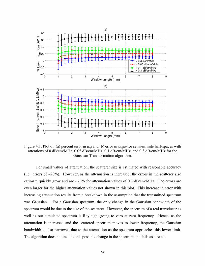
Figure 4.1: Plot of (a) percent error in aeff and (b) error in αeffzT for semi-infinite half-spaces with
attentions of 0 dB/cm/MHz, 0.05 dB/cm/MHz, 0.1 dB/cm/MHz, and 0.3 dB/cm/MHz for the Gaussian Transformation algorithm.
For small values of attenuation, the scatterer size is estimated with reasonable accuracy
(i.e., errors of ~20%). However, as the attenuation is increased, the errors in the scatterer size
estimate quickly grow and are ~70% for attenuation values of 0.3 dB/cm/MHz. The errors are
even larger for the higher attenuation values not shown in this plot. This increase in error with
increasing attenuation results from a breakdown in the assumption that the transmitted spectrum
was Gaussian. For a Gaussian spectrum, the only change in the Gaussian bandwidth of the
spectrum would be due to the size of the scatterer. However, the spectrum of a real transducer as
well as our simulated spectrum is Rayleigh, going to zero at zero frequency. Hence, as the
attenuation is increased and the scattered spectrum moves to lower frequency, the Gaussian
bandwidth is also narrowed due to the attenuation as the spectrum approaches this lower limit.
The algorithm does not include this possible change in the spectrum and fails as a result.
64
One modification to the algorithm that was also considered to correct for this failing
involved replacing the Gaussian spectrum approximation with a modified Rayleigh spectrum
approximation. The derivation leading to Equation (4.4) would remain the same except for a
multiplication of |f|4 before the exponential. Then, the change in bandwidth would be found by
fitting a modified Rayleigh distribution to the appropriate measured spectrum and solving for the
scatterer size appropriately. Unfortunately, fitting Rayleigh distributions to the measured
spectrum was not a robust operation. Hence, changes in the attenuation still resulted in
inappropriate changes in the bandwidth, and the algorithm still failed.
Despite the algorithm’s sensitivity to attenuation it was informative to also test the
algorithm’s sensitivity to noise. As a result, the attenuation was maintained at 0.05 dB/cm/MHz
and various levels of white Gaussian noise were added to each of the waveforms from the
scatterers in the time domain. For each noise level, the scatterer sizes/attentions were found and
compared to the mean scatterer size/attenuation found for the noiseless case. The resulting
differences between the cases are shown in Figure 4.2. In this plot, the vertical error bars are the
same as those given in Equations (4.18) and (4.19), and the horizontal error bars correspond to
one standard deviation of the calculated SNR values from each of the 40 estimates. The SNR
values for each estimate were calculated from
SNRg t v t dt
g t v t dt
win refl
win noisej
j= ⋅F
HGG
I
KJJ
F
HGG
I
KJJ
zz∑
=
125
10
2
21
25
logb g b ge jb g b gc h
(4.20)
where are the RF echoes from each group of 25 used in the estimate before the noise has
been added, and v
vrefl j
noise is the noise signal used to obtain the estimate for E . The
difference between the estimates is small for SNRs as low as 8 dB.
N N fb g 2
4.5 Chapter Summary
In this chapter, the performance of the Gaussian Transformation algorithm was assessed
for determining the total attenuation and scatterer size simultaneously. Although the algorithm’s
performance was reasonable for very small attentions, the accuracy of the scatterer size estimate
quickly degraded with increasing attenuation. The failure was a result of the algorithm assuming
that the spectrum was perfectly Gaussian when in fact real spectra are better described by a
65
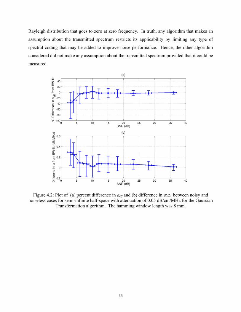
Rayleigh distribution that goes to zero at zero frequency. In truth, any algorithm that makes an
assumption about the transmitted spectrum restricts its applicability by limiting any type of
spectral coding that may be added to improve noise performance. Hence, the other algorithm
considered did not make any assumption about the transmitted spectrum provided that it could be
measured.
Figure 4.2: Plot of (a) percent difference in aeff and (b) difference in αozT between noisy and
noiseless cases for semi-infinite half-space with attenuation of 0.05 dB/cm/MHz for the Gaussian Transformation algorithm. The hamming window length was 8 mm.
66
CHAPTER 5
SPECTRAL FIT ALGORITHM
The Gaussian Transformation algorithm presented in Chapter 4 failed because it made an
assumption about the transmitted spectrum that was not accurate. Hence, the second algorithm
involved solving for both the total attenuation and the scatterer size using a single minimization
routine to fit a curve to the backscattered spectrum without making any assumptions about the
form of the scattered spectrum and was termed the Spectral Fit algorithm. In this chapter, the
Spectral Fit algorithm will be introduced and several modifications to the algorithm will be
discussed.
5.1 Basic Spectral Fit Algorithm
Initially, the Spectral Fit algorithm was implemented using many of the same processing
techniques introduced in the Gaussian Transformation algorithm. Weakly focused transducers,
“small” window lengths, and a linear frequency dependence of the attenuation along the
propagation path were assumed, so that Acomp could be approximated as e zT o4 fα . Then, Pscat was
found by averaging the spectra from 25 independent RF echoes in the log domain according to
Equation (4.6), and the effects of electronic noise were reduced by dividing by
12
+FH IKE N f P fN scat measuredb g b g as was described in Chapter 4. Hence,
P fV
E N f Vscat
ii
N ii
b ge j
b g e j=
FHG
IKJ
+FHG
IKJ
FHG
IKJ
=
=
∑
∑
exp ln
exp ln
125
1 125
2
1
25
2 2
1
25 (5.1)
in the first implementation of the algorithm. Also, the echo signal from a rigid plane positioned
at the focus was simulated, windowed by the same hamming window used to window the
simulated backscattered signal, and multiplied by k yielding o4
67
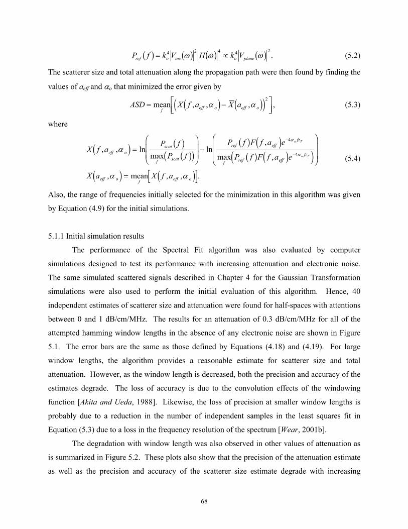
P f k V H k Vref o inc o planeb g b g b g b g= ∝4 2 4 4 2ω ω ω . (5.2)
The scatterer size and total attenuation along the propagation path were then found by finding the
values of aeff and αo that minimized the error given by
ASD X f a X af eff o eff o= −LNM
OQPmean , , ,α αd i de 2ij , (5.3)
where
X f aP f
P f
P f F f a e
P f F f a e
X a X f a
eff oscat
f scat
ref efffz
f ref efffz
eff o f eff o
o T
o T, , ln
maxln
,
max ,
, mean , , .
α
α α
α
αd i b gb gc h
b g d ib g d ie j
d i d i
=FHGG
IKJJ −F
HGG
I
KJJ
=
−
−
4
4 (5.4)
Also, the range of frequencies initially selected for the minimization in this algorithm was given
by Equation (4.9) for the initial simulations.
5.1.1 Initial simulation results
The performance of the Spectral Fit algorithm was also evaluated by computer
simulations designed to test its performance with increasing attenuation and electronic noise.
The same simulated scattered signals described in Chapter 4 for the Gaussian Transformation
simulations were also used to perform the initial evaluation of this algorithm. Hence, 40
independent estimates of scatterer size and attenuation were found for half-spaces with attentions
between 0 and 1 dB/cm/MHz. The results for an attenuation of 0.3 dB/cm/MHz for all of the
attempted hamming window lengths in the absence of any electronic noise are shown in Figure
5.1. The error bars are the same as those defined by Equations (4.18) and (4.19). For large
window lengths, the algorithm provides a reasonable estimate for scatterer size and total
attenuation. However, as the window length is decreased, both the precision and accuracy of the
estimates degrade. The loss of accuracy is due to the convolution effects of the windowing
function [Akita and Ueda, 1988]. Likewise, the loss of precision at smaller window lengths is
probably due to a reduction in the number of independent samples in the least squares fit in
Equation (5.3) due to a loss in the frequency resolution of the spectrum [Wear, 2001b].
The degradation with window length was also observed in other values of attenuation as
is summarized in Figure 5.2. These plots also show that the precision of the attenuation estimate
as well as the precision and accuracy of the scatterer size estimate degrade with increasing
68

attenuation. However, consistently reasonable estimates with errors in scatterer size less than
20% are still obtainable for attenuations as high as 0.6 dB/cm/MHz at a window length of 8 mm.
Figure 5.1: Errors in estimated (a) scatterer size and (b) total attenuation for different hamming
window lengths for an attenuation of 0.3 dB/cm/MHz in the absence of any electronic noise.
Figure 5.2: Plot of errors in estimated (a) scatterer size and (b) total attenuation for different
values of attenuation with hamming window lengths of (I) 2 mm, (II) 4 mm, and (III) 8 mm in the absence of any electronic noise.
69
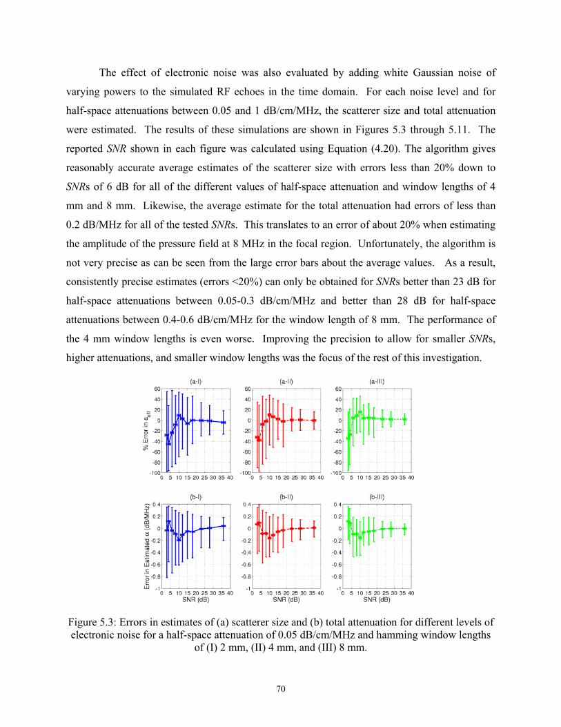
The effect of electronic noise was also evaluated by adding white Gaussian noise of
varying powers to the simulated RF echoes in the time domain. For each noise level and for
half-space attenuations between 0.05 and 1 dB/cm/MHz, the scatterer size and total attenuation
were estimated. The results of these simulations are shown in Figures 5.3 through 5.11. The
reported SNR shown in each figure was calculated using Equation (4.20). The algorithm gives
reasonably accurate average estimates of the scatterer size with errors less than 20% down to
SNRs of 6 dB for all of the different values of half-space attenuation and window lengths of 4
mm and 8 mm. Likewise, the average estimate for the total attenuation had errors of less than
0.2 dB/MHz for all of the tested SNRs. This translates to an error of about 20% when estimating
the amplitude of the pressure field at 8 MHz in the focal region. Unfortunately, the algorithm is
not very precise as can be seen from the large error bars about the average values. As a result,
consistently precise estimates (errors <20%) can only be obtained for SNRs better than 23 dB for
half-space attenuations between 0.05-0.3 dB/cm/MHz and better than 28 dB for half-space
attenuations between 0.4-0.6 dB/cm/MHz for the window length of 8 mm. The performance of
the 4 mm window lengths is even worse. Improving the precision to allow for smaller SNRs,
higher attenuations, and smaller window lengths was the focus of the rest of this investigation.
Figure 5.3: Errors in estimates of (a) scatterer size and (b) total attenuation for different levels of electronic noise for a half-space attenuation of 0.05 dB/cm/MHz and hamming window lengths
of (I) 2 mm, (II) 4 mm, and (III) 8 mm.
70
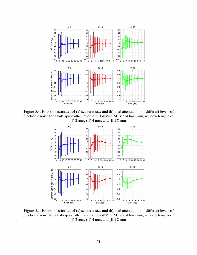
Figure 5.4: Errors in estimates of (a) scatterer size and (b) total attenuation for different levels of electronic noise for a half-space attenuation of 0.1 dB/cm/MHz and hamming window lengths of
(I) 2 mm, (II) 4 mm, and (III) 8 mm.
Figure 5.5: Errors in estimates of (a) scatterer size and (b) total attenuation for different levels of electronic noise for a half-space attenuation of 0.2 dB/cm/MHz and hamming window lengths of
(I) 2 mm, (II) 4 mm, and (III) 8 mm.
71
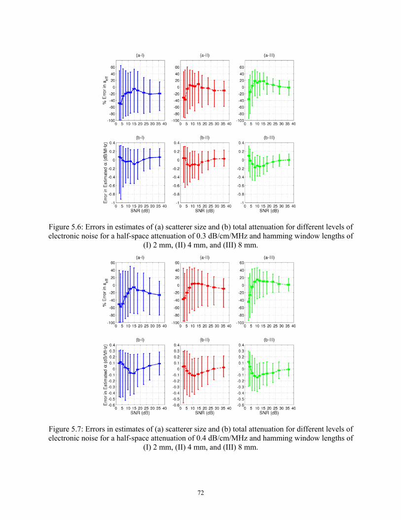
Figure 5.6: Errors in estimates of (a) scatterer size and (b) total attenuation for different levels of electronic noise for a half-space attenuation of 0.3 dB/cm/MHz and hamming window lengths of
(I) 2 mm, (II) 4 mm, and (III) 8 mm.
Figure 5.7: Errors in estimates of (a) scatterer size and (b) total attenuation for different levels of electronic noise for a half-space attenuation of 0.4 dB/cm/MHz and hamming window lengths of
(I) 2 mm, (II) 4 mm, and (III) 8 mm.
72
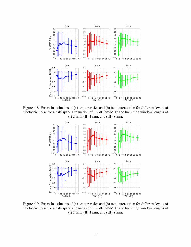
Figure 5.8: Errors in estimates of (a) scatterer size and (b) total attenuation for different levels of electronic noise for a half-space attenuation of 0.5 dB/cm/MHz and hamming window lengths of
(I) 2 mm, (II) 4 mm, and (III) 8 mm.
Figure 5.9: Errors in estimates of (a) scatterer size and (b) total attenuation for different levels of electronic noise for a half-space attenuation of 0.6 dB/cm/MHz and hamming window lengths of
(I) 2 mm, (II) 4 mm, and (III) 8 mm.
73
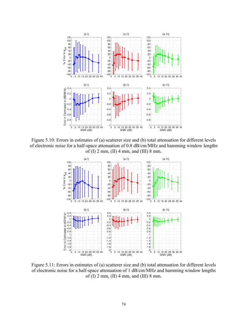
Figure 5.10: Errors in estimates of (a) scatterer size and (b) total attenuation for different levels
of electronic noise for a half-space attenuation of 0.8 dB/cm/MHz and hamming window lengths of (I) 2 mm, (II) 4 mm, and (III) 8 mm.
Figure 5.11: Errors in estimates of (a) scatterer size and (b) total attenuation for different levels of electronic noise for a half-space attenuation of 1 dB/cm/MHz and hamming window lengths
of (I) 2 mm, (II) 4 mm, and (III) 8 mm.
74

5.2 Modifications to the Basic Spectral Fit Algorithm
While the Spectral Fit algorithm was being tested, some of the processing steps were
evaluated and improved. Hence, before concluding this chapter, several modifications to the
algorithm need to be discussed.
5.2.1 Noise reduction techniques
The first processing steps evaluated involved those associated with reducing the noise
before performing the estimate. First, recall from Chapter 4 that the spectral noise resulting from
the random scatterer spacing was reduced by averaging the spectra of the 25 pulse-echo
waveforms in the log domain as given by Equation (4.6). Traditionally, however, the averaging
of the spectra is done in the regular frequency domain [Insana et al., 1990] or
P f Vscat jj
b g ==∑1
252
1
25
. (5.5)
A comparison of the two averaging methods is provided in Figure 5.12 for a half-space
attenuation of 0.3 dB/cm/MHz in the absence of any electronic noise. The mean values of the
estimates are almost identical, but the deviation in the estimates, given by adding together the
upper and lower error bars, is slightly larger when averaging in the log domain. Hence, one
method to reduce the variance in the estimator in future algorithms would be to average in the
normal spectral domain rather than the log domain.
The second noise reduction technique evaluated was the division of the averaged
spectrum by 12
+FH IKE N scat measuredN f P fb g b g to reduce the impact of electronic noise. The
evaluation was done by comparing the results for three different levels of electronic noise both
with and without the compensating term for a half-space with an attenuation of 0.05
dB/cm/MHz. The errors in the average estimates are shown in Figure 5.13. In this evaluation,
the averaging of the 25 spectra was still done in the log domain. From Figure 5.13, it is clear that
the electronic noise compensation term 12
+FH IKE N scat measuredN f P fb g b g greatly improves the
accuracy of the estimates in the presence of electronic system noise.
75
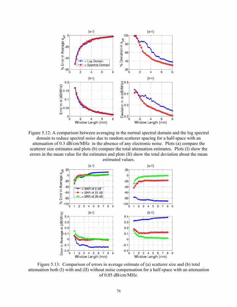
Figure 5.12: A comparison between averaging in the normal spectral domain and the log spectral
domain to reduce spectral noise due to random scatterer spacing for a half-space with an attenuation of 0.3 dB/cm/MHz in the absence of any electronic noise. Plots (a) compare the
scatterer size estimates and plots (b) compare the total attenuation estimates. Plots (I) show the errors in the mean value for the estimates and plots (II) show the total deviation about the mean
estimated values.
Figure 5.13: Comparison of errors in average estimate of (a) scatterer size and (b) total
attenuation both (I) with and (II) without noise compensation for a half-space with an attenuation of 0.05 dB/cm/MHz.
76

Although tested when averaging in the log domain, the error correction term would still
apply when averaging in the normal spectral domain because Equation (4.14) would become
P f V fE N f
V f
V f E N f
P fE N f
P f
scat i
N
ii
ii
N
scat ideal
N
scat ideal
b g b gb gb g
b g b g
b gb gb g
= +F
HGG
I
KJJ
F
HGGG
I
KJJJ
= +
= +F
HGG
I
KJJ
=
=
∑
∑
125
1
125
1
2
2
21
25
2
1
25 2
2
.
(5.6)
Hence,
P fP f
E N f
P f
scat ideal
scat measured
N
scat measured
b g b gb gb g
≅
+F
HGG
I
KJJ1
2 (5.7)
indicating that dividing by 12
+FH IKE N scat measuredN f P fb g b g should still decrease the impact of
electronic noise. This hypothesis is validated in Section 5.2.3.
5.2.2 Windowing function compensation
In the initial algorithms considered, compensating for the effects of windowing (i.e.
blurring of the spectrum) was done by applying the same window of length L to both the
reference signal and the backscattered signal while accounting for the difference in sound speed.
Also, a hamming window was used to perform the windowing. However, it is not clear that this
is the best approach. Therefore, in this section, other windowing schemes and compensation
methods are considered within the framework of the Spectral Fit algorithm. The algorithm
remains the same as discussed in Section 5.1 with the exception that the spectra from adjacent
RF echoes are averaged in the regular frequency domain instead of the log frequency domain.
Initially, three different simulations were preformed using the same type of half-space
described previously with an attenuation of 0.3 dB/cm/MHz without any electronic noise added.
In the first simulation, both the reference waveform and the backscattered waveforms were
windowed with hamming windows with the same length L, as was done previously. Then, both
77
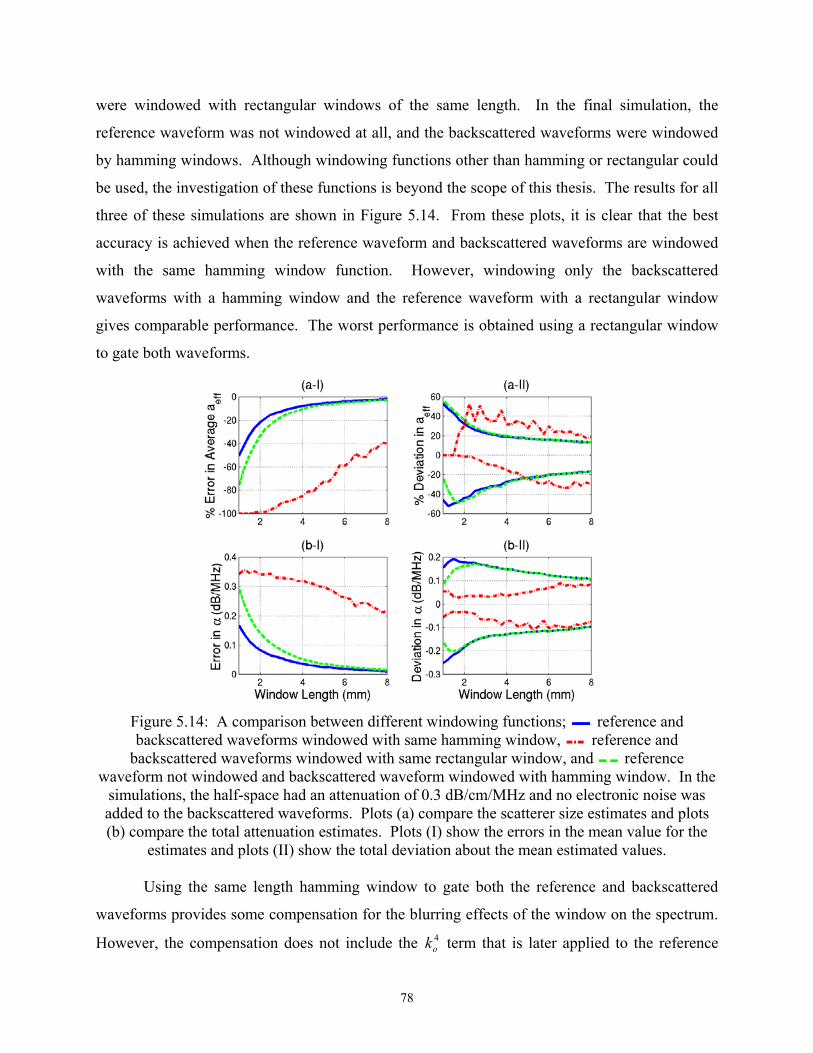
were windowed with rectangular windows of the same length. In the final simulation, the
reference waveform was not windowed at all, and the backscattered waveforms were windowed
by hamming windows. Although windowing functions other than hamming or rectangular could
be used, the investigation of these functions is beyond the scope of this thesis. The results for all
three of these simulations are shown in Figure 5.14. From these plots, it is clear that the best
accuracy is achieved when the reference waveform and backscattered waveforms are windowed
with the same hamming window function. However, windowing only the backscattered
waveforms with a hamming window and the reference waveform with a rectangular window
gives comparable performance. The worst performance is obtained using a rectangular window
to gate both waveforms.
Figure 5.14: A comparison between different windowing functions; reference and backscattered waveforms windowed with same hamming window, reference and
backscattered waveforms windowed with same rectangular window, and reference waveform not windowed and backscattered waveform windowed with hamming window. In the
simulations, the half-space had an attenuation of 0.3 dB/cm/MHz and no electronic noise was added to the backscattered waveforms. Plots (a) compare the scatterer size estimates and plots (b) compare the total attenuation estimates. Plots (I) show the errors in the mean value for the
estimates and plots (II) show the total deviation about the mean estimated values.
Using the same length hamming window to gate both the reference and backscattered
waveforms provides some compensation for the blurring effects of the window on the spectrum.
However, the compensation does not include the k term that is later applied to the reference o4
78
spectrum from the plate. Therefore, to improve the performance of the algorithm at smaller
window lengths other compensation techniques need to be considered. One possibility would be
to use a reference phantom instead of a rigid plane at the focus to obtain the reference spectrum
[Gerig et al., 2003] and then use the same hamming window on both. However, a reference
phantom will increase the uncertainty of the estimation technique [Gerig et al., 2003].
Furthermore, it is difficult to perform a comprehensive evaluation of the reference phantom
technique due to the need to test materials with attenuation, scatterer type, and scatterer sizes
differing from the reference phantom. Hence, the reference phantom technique was not
evaluated at this time. Instead, an attempt was made to directly compensate for the windowing
effects on the backscattered waveforms while still using a rigid plane placed at the focus as a
reference.
It has been shown that windowing of the signals in the time domain is equivalent to a
convolution of the power spectra given by [Wear, 2002]
E E *V V Greflwindowed
reflideal
win
2 2 2∝ b gf , (5.8)
where is the Fourier transform of the windowing function. Also, if the windowing
function and expected backscattered spectra can be reasonably described by Gaussian
distributions given by
G fwin b g
E e
e ,
V
G f
reflideal
f f
win
f
o
g
2 2
2 2
2
2
2
2
∝
∝
−−
−
b g
b g
σ
σ
ω
(5.9)
then the windowed backscattered spectrum is approximately given by [Wear, 2002]
E eVreflwindowed
f fo
g2 2
2
2 2
∝−
−
+
b geσ σω j . (5.10)
Hence, the windowing will increase the bandwidth of the backscattered waveform leading to an
underestimate of the scatterer size for smaller window lengths as was observed in the above
results. Furthermore, the broadening, as described in this manner, can be compensated by
multiplying the windowed spectrum by
Gcorr
f fo g
g=−
−
+eb ge j
2 2
2 2 22
σ
σ σ σω ω . (5.11)
79
This correction for windowing was tested by a simulation assuming a half-space as described
above with an attenuation of 0.3 dB/cm/MHz. The backscattered spectrum from 25 independent
RF echoes windowed with hamming windows without any additive electronic noise were
averaged together in the normal frequency domain yielding E . The resulting
average spectrum was then fit by a Gaussian distribution in the log domain, as is discussed in
Chapter 4, to obtain values for f
Vreflwindowed
2
o and d . The Fourier transform of the hamming window
was also calculated and fit by a Gaussian distribution in the normal frequency domain to obtain
the value of
σ σω2 + g
2 i
σ g2 . Gcorr was then calculated and applied from these parameters. Because the
effects of windowing on the backscattered spectrum were directly compensated, no windowing
was applied to the reference spectrum from the rigid plane. The results of this simulation are
shown with the results using a hamming window for both the reference and backscattered signals
from before in Figure 5.15. Clearly, the correction term allows for accurate estimates of total
attenuation and scatterer size down to window lengths of 1 mm. However, the precision of the
estimates continues to degrade for the smaller window lengths.
Instead of correcting for the windowing after averaging the spectra from the 25
independent RF echoes, it is also possible to apply the correction to each RF echo individually
before averaging. Therefore, the simulation was repeated with Gcorr being found and applied
before the spectra were averaged using the updated frequency range described in the next
section. The results for finding and applying Gcorr both before and after averaging are shown in
Figure 5.16. From Figure 5.16, it is clear that the blurring effect of windowing should be
corrected after the spectra have been averaged together in the frequency domain.
5.2.3 Updating frequency range used for fit
In the earlier simulations, the frequency range used by the algorithm was dictated by
Equation (4.9). However, this definition of the frequency range is not robust and depends
heavily on the sampling rate used to acquire the data. Therefore, before the algorithms can be
reliably implemented by other investigators, a better definition of the usable frequency range
needs to be obtained. Because the whole purpose in selecting the frequency range is to exclude
spectral regions dominated by system noise, a suitable alternative would be to select only those
frequencies whose signal levels were reasonably larger than the noise floor. Hence, a more
80
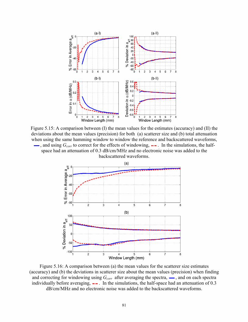
Figure 5.15: A comparison between (I) the mean values for the estimates (accuracy) and (II) the deviations about the mean values (precision) for both (a) scatterer size and (b) total attenuation when using the same hamming window to window the reference and backscattered waveforms,
, and using Gcorr to correct for the effects of windowing, . In the simulations, the half-space had an attenuation of 0.3 dB/cm/MHz and no electronic noise was added to the
backscattered waveforms.
Figure 5.16: A comparison between (a) the mean values for the scatterer size estimates
(accuracy) and (b) the deviations in scatterer size about the mean values (precision) when finding and correcting for windowing using Gcorr after averaging the spectra, , and on each spectra individually before averaging, . In the simulations, the half-space had an attenuation of 0.3
dB/cm/MHz and no electronic noise was added to the backscattered waveforms.
81

generalized selection criteria for the proper frequency range to perform the estimates is given by
the set of all frequencies corresponding to signal levels greater than
N NP f f
P fFloor dB
scat N N
f scat Gaussianfit
= FHG
IKJ
F
H
GGGG
I
K
JJJJ
F
H
GGGG
I
K
JJJJ+
L
N
MMMMM
O
Q
PPPPP
F
H
GGGGG
I
K
JJJJJ−
∀
max mean log:
max10 6200b g
b gm r, (5.12)
where NdB sets a limit on the frequency range in the absence of any electronic noise and fN refers
to the largest positive frequency after taking the DFT of the sampled waveforms. In the
simulations, NdB was set to either –20 dB or –30 dB, and the signal was sufficiently oversampled
so that at least the last 200 frequency samples would correspond to the additive white electronic
system noise. Hence, Equation (5.10) only uses signal frequencies greater than 6 dB above the
noise floor.
EN N fb g 2 used in compensating for the electronic noise by dividing the received
spectrum by the term 12
+FH IKE N f V fN scat measuredb g b g might also be obtainable from
, removing the need to record the noise in the absence of a transmitted signal. In
order to test this possibility, the simulation results given in Figure 5.13 were repeated using
P f fscat N N−200:b g
EN N fb g 2 obtained from both a reference noise signal as well as by averaging the last 200
values of Pscat. In addition, the convolution effects of windowing were compensated and the
frequency range used in the minimization was given by Equation (5.12) with NdB set to –20 dB.
The results for both methods of obtaining E are shown in Figure 5.17 along with the
results obtained without any electronic noise compensation. Both methods for obtaining an
estimate for
N N fb g 2
E perform about the same and give significant improvement in the
accuracy compared to when the electronic noise is not compensated validating the hypothesis
from Section 5.2.1. Due to the comparable performance, in the future
N N fb g 2
E will be found
from the last 200 values of P
N N fb g 2
scat, removing the need to record the noise in the absence of a
transmitted signal.
82

Figure 5.17: Comparison of errors in scatterer size estimates for SNRs of (a) 9 dB, (b) 23 dB, and (c) 36 dB as well as attenuation estimates for SNRs of (d) 9 dB, (e) 23 dB, and (f) 36 dB without noise compensation and with different methods for estimating E for a half-space with
an attenuation of 0.05 dB/cm/MHz. N N fb g 2
5.3 Chapter Summary
In this chapter, the performance of the basic Spectral Fit algorithm for determining the
total attenuation and scatterer size simultaneously was assessed. The performance of the basic
Spectral Fit algorithm was reasonable for attenuations less than 0.8 dB/cm/MHz, SNRs for 23 dB
to 28 dB, and window lengths of 8 mm. The limiting factor of the performance was a lack of
precision with increasing noise, decreasing window length, and increasing attenuation. Hence,
Chapters 6 and 7 will focus on improving the precision of the estimator. Also, several
modifications to the basic Spectral Fit algorithm were evaluated. First, a comparison of
averaging the pulse echo waveforms in the log spectral domain was compared to the averaging
of the waveforms in the traditional spectral domain and found to be slightly less precise.
Likewise, the electronic noise compensation term was evaluated and found to yield a significant
improvement on the accuracy of the estimates. Then, the blurring effects of windowing were
corrected assuming that the backscattered spectrum could be reasonably approximated as a
Gaussian distribution. Lastly, a new criterion for selecting the frequency range over which the
Spectral Fit algorithm would perform the required minimization was explained.
83

CHAPTER 6
SIGNAL PROCESSING TECHNIQUES TO IMPROVE PRECISION OF SPECTRAL FIT ALGORITHM
After developing the Spectral Fit algorithm, many different signal processing techniques
were investigated with the goal of improving the precision of the estimation scheme. In this
chapter, each of the attempted signal processing techniques is discussed.
6.1 Growing Window Averaging
The first signal processing technique investigated was a simple extension of the Spectral
Fit algorithm where the estimates for any given window size were the average of the estimates
for smaller window sizes. In the algorithm, the averaging was restricted to window lengths
greater than 2 mm. Furthermore, because scatterer size estimates of less than 1 µm were not
physically reasonable for the range of frequencies used in the evaluation, any estimates giving a
scatterer size smaller than 1 µm were also excluded from the averaging. Because estimates for
window lengths have already been found for the basic Spectral Fit algorithm in Chapter 5, the
same data were re-evaluated using this new algorithm. As a result, the spectra were still
averaged in the log domain and the convolution effects of windowing remained uncompensated.
Despite these limitations, the general performance of the algorithm could still be evaluated.
Also, the choice of limiting the window length in the averaging to 2 mm was somewhat arbitrary.
Hence, other limits may have slightly different performances, but the general behavior should
not be drastically affected.
A plot showing the errors in the estimated total attenuation and scatterer size for the half-
space with an attenuation of 0.3 dB/cm/MHz for the attempted window lengths is shown in
Figure 6.1. Because scatterer estimates of less than 1 µm were automatically excluded from the
averaging, not all 40 of the independent waveform groups yielded an estimate as is shown in
Figure 6.1c. Also, when comparing the results shown in Figure 6.1 to the previous results given
84
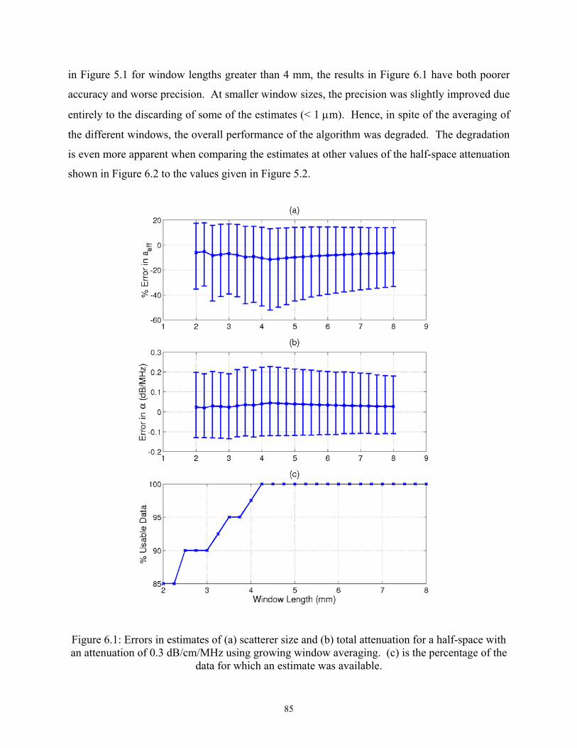
in Figure 5.1 for window lengths greater than 4 mm, the results in Figure 6.1 have both poorer
accuracy and worse precision. At smaller window sizes, the precision was slightly improved due
entirely to the discarding of some of the estimates (< 1 µm). Hence, in spite of the averaging of
the different windows, the overall performance of the algorithm was degraded. The degradation
is even more apparent when comparing the estimates at other values of the half-space attenuation
shown in Figure 6.2 to the values given in Figure 5.2.
Figure 6.1: Errors in estimates of (a) scatterer size and (b) total attenuation for a half-space with an attenuation of 0.3 dB/cm/MHz using growing window averaging. (c) is the percentage of the
data for which an estimate was available.
85
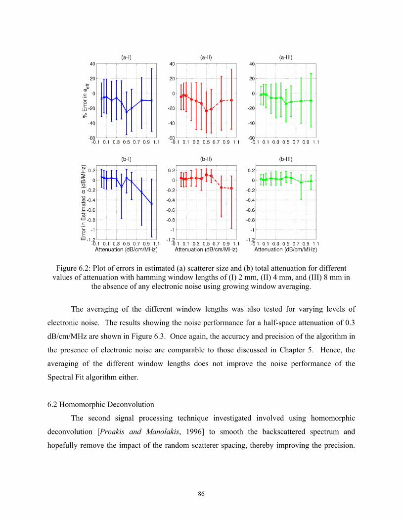
Figure 6.2: Plot of errors in estimated (a) scatterer size and (b) total attenuation for different
values of attenuation with hamming window lengths of (I) 2 mm, (II) 4 mm, and (III) 8 mm in the absence of any electronic noise using growing window averaging.
The averaging of the different window lengths was also tested for varying levels of
electronic noise. The results showing the noise performance for a half-space attenuation of 0.3
dB/cm/MHz are shown in Figure 6.3. Once again, the accuracy and precision of the algorithm in
the presence of electronic noise are comparable to those discussed in Chapter 5. Hence, the
averaging of the different window lengths does not improve the noise performance of the
Spectral Fit algorithm either.
6.2 Homomorphic Deconvolution
The second signal processing technique investigated involved using homomorphic
deconvolution [Proakis and Manolakis, 1996] to smooth the backscattered spectrum and
hopefully remove the impact of the random scatterer spacing, thereby improving the precision.
86
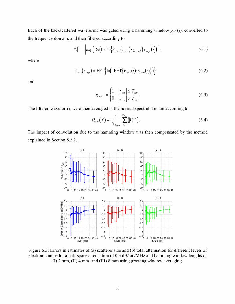
Each of the backscattered waveforms was gated using a hamming window gwin(t), converted to
the frequency domain, and then filtered according to
V V gi cep i cep win cep2
2
2
= ⋅exp Re IFFT τ τd i d ioee jtj , (6.1)
where
V v tcepi cep refl i winτd i b g b gne= FFT ln IFFT g t s j⋅ (6.2)
and
gTTwin
cep cep
cep cep2
10
=≤
>
RS|T|
ττ
. (6.3)
The filtered waveforms were then averaged in the normal spectral domain according to
P fN
Vscatlines
ii
Nlinesb g e==∑1 2
1j . (6.4)
The impact of convolution due to the hamming window was then compensated by the method
explained in Section 5.2.2.
Figure 6.3: Errors in estimates of (a) scatterer size and (b) total attenuation for different levels of electronic noise for a half-space attenuation of 0.3 dB/cm/MHz and hamming window lengths of
(I) 2 mm, (II) 4 mm, and (III) 8 mm using growing window averaging.
87

In order to test the algorithm, simulations were performed of a spherically focused f/4
transducer with a focal length of 5 cm sonifying an infinite half-space as was described in
Chapter 5. The only difference being that this time 2000 random scatterer distributions were
generated. The waveforms from each distribution were then initially grouped in sets of 40 to
yield 50 independent estimates of scatterer size and total attenuation at each hamming window
length (varied from 1 to 8 mm). The waveforms were initially taken in sets of 40 instead of 25 to
attempt to further improve the precision. The relationship between varying the number of
waveforms in each set and precision will be discussed later in this section. In addition, the code
used a sampling rate of 160 MHz when “digitizing” the signal, and the attenuation of the half-
space region was kept at 0.3 dB/cm/MHz. The range of frequencies used by the minimization
scheme to perform the estimate was selected so that every frequency f used in the fit satisfied
10 20 10 6200logmax
max mean log:
max
P f
P f
P f f
P f
scat
f scat Gaussianfit
scat N N
f scat Gaussianfit
b gb gm r
b gb gm r
∀
−
∀
FHG
IKJ
F
H
GGGG
I
K
JJJJ> − F
HGIKJ
F
H
GGGG
I
K
JJJJ
F
H
GGGG
I
K
JJJJ+
L
N
MMMMM
O
Q
PPPPP
F
H
GGGGG
I
K
JJJJJ (6.5)
(i.e., 6 dB above the noise floor with a maximum set to the –20 dB bandwidth).
In the simulations, the value of Tcep used to set the amount of filtering was varied as 0.15
µs, 0.31 µs, 0.46 µs, and 0.62 µs. The locations of all of these cutoffs relative to the main
spectral peak are shown with an example signal plotted in the cepstrum domain in Figure 6.4
along with the original unfiltered spectrum. After applying the filter in the cepstrum domain, the
example spectra have been significantly smoothed as is shown in Figure 6.5. The smaller the
value of Tcep, the greater the filtering, and the smoother the resulting spectra. The simulation
results for the four different filter lengths are shown in Figure 6.6. For a filter length of 0.15 µs,
the accuracy of the scatterer size estimates has been seriously degraded, especially for small
window lengths. Hence, this filter length will not be considered in our more detailed analysis of
the accuracy and precision given in Figure 6.7. In addition to simulating each of the four filtered
cases, the simulation was also run without filtering (i.e., Tcep = ∞ ). Hence, the performance of
the filtered cases could be compared with the performance available from the straight Spectral
Fit algorithm with 40 waveforms in each set averaged in the normal spectral domain while
compensating for the convolution effects of windowing.
88

Figure 6.4: (a) Example spectrum for a single RF echo in cepstrum domain showing
locations of Tcep cutoffs used in the homomorphic deconvolution with (b) the corresponding normalized spectra before any homomorphic processing has been applied.
Figure 6.5: Example normalized spectrum for a single RF echo after applying homomorphic
deconvolution with (a) Tcep = 0.15 µs, (b) Tcep = 0.31 µs, (c) Tcep = 0.46 µs, and (d) Tcep = 0.62 µs.
89
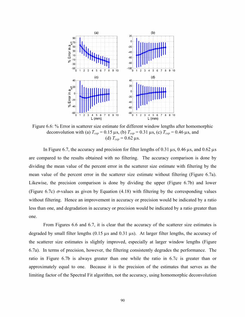
Figure 6.6: % Error in scatterer size estimate for different window lengths after homomorphic
deconvolution with (a) Tcep = 0.15 µs, (b) Tcep = 0.31 µs, (c) Tcep = 0.46 µs, and (d) Tcep = 0.62 µs.
In Figure 6.7, the accuracy and precision for filter lengths of 0.31 µs, 0.46 µs, and 0.62 µs
are compared to the results obtained with no filtering. The accuracy comparison is done by
dividing the mean value of the percent error in the scatterer size estimate with filtering by the
mean value of the percent error in the scatterer size estimate without filtering (Figure 6.7a).
Likewise, the precision comparison is done by dividing the upper (Figure 6.7b) and lower
(Figure 6.7c) σ-values as given by Equation (4.18) with filtering by the corresponding values
without filtering. Hence an improvement in accuracy or precision would be indicated by a ratio
less than one, and degradation in accuracy or precision would be indicated by a ratio greater than
one.
From Figures 6.6 and 6.7, it is clear that the accuracy of the scatterer size estimates is
degraded by small filter lengths (0.15 µs and 0.31 µs). At larger filter lengths, the accuracy of
the scatterer size estimates is slightly improved, especially at larger window lengths (Figure
6.7a). In terms of precision, however, the filtering consistently degrades the performance. The
ratio in Figure 6.7b is always greater than one while the ratio in 6.7c is greater than or
approximately equal to one. Because it is the precision of the estimates that serves as the
limiting factor of the Spectral Fit algorithm, not the accuracy, using homomorphic deconvolution
90
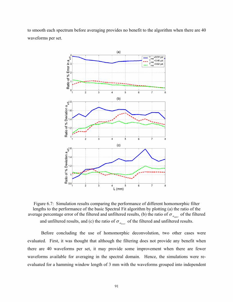
to smooth each spectrum before averaging provides no benefit to the algorithm when there are 40
waveforms per set.
Figure 6.7: Simulation results comparing the performance of different homomorphic filter lengths to the performance of the basic Spectral Fit algorithm by plotting (a) the ratio of the
average percentage error of the filtered and unfiltered results, (b) the ratio of σ aupper of the filtered
and unfiltered results, and (c) the ratio of σ alower of the filtered and unfiltered results.
Before concluding the use of homomorphic deconvolution, two other cases were
evaluated. First, it was thought that although the filtering does not provide any benefit when
there are 40 waveforms per set, it may provide some improvement when there are fewer
waveforms available for averaging in the spectral domain. Hence, the simulations were re-
evaluated for a hamming window length of 3 mm with the waveforms grouped into independent
91

sets of 2, 5, 10, and 25 waveforms. For the sake of comparison, a total of 50 estimates were
made for each of the different waveform groupings. Hence, not all 2000 of the previously
generated waveforms were needed. Figure 6.8 shows the precision results for each grouping of
the waveforms where the upper and lower σ-values from Equation (4.18) are plotted above and
below the axis respectively. The first bar in each group corresponds to the case where no
homomorphic filtering was applied to the waveforms while the second, third, fourth, and fifth
bars correspond to results for filter lengths of 0.15 µs, 0.31 µs, 0.46 µs, and 0.62 µs, respectively.
Figure 6.8: σ aupper
and σ alower values when a different number of waveforms are averaged in each
set before perfroming the estimate for the different homomorphic deconvolution parameters.
In Figure 6.8, there is a systematic improvement in precision as the number of
independent waveforms used to obtain the estimate is increased. However, for a given number
of waveforms in a set, there is no improvement in precision provided by homomorphic
deconvolution. The only possible exception occurs when there are only two waveforms per set,
but the overall precision for this case is so poor that the amount of improvement is insignificant.
Hence, homomorphic deconvolution will not allow for fewer waveforms to be used in the
estimation scheme for the same level of precision.
The final case considered before concluding the consideration of homomorphic
deconvolution involved applying the filtering to the spectra after averaging the 40 independent
waveforms in the normal spectral domain rather than applying the filtering to each waveform
92

individually. Once again, the value of Tcep used to set the amount of filtering was varied as 0.15
µs, 0.31 µs, 0.46 µs, and 0.62 µs, and the simulation was also run without filtering (i.e.,
Tcep = ∞ ). In Figure 6.9, the accuracy and precision for the different filter lengths applied after
averaging are compared to the results obtained with no filtering as was done previously. Hence,
the accuracy comparison is done by dividing mean value of the percent error in the scatterer size
estimate with filtering by mean value of the percent error in the scatterer size estimate without
filtering (Figure 6.9a). Likewise, the precision comparison is done by dividing the upper (Figure
6.9b) and lower (Figure 6.9c) σ-values as given by Equation (4.18) with filtering by the
corresponding values without filtering. The accuracy of the estimates is still slightly degraded
by the filtering for small filter lengths, and the accuracy is still improved at larger filter lengths
and window lengths greater than 3 mm. However, the precision of the estimates is relatively
unaffected by the filtering. Hence, using homomorphic deconvolution to smooth each spectrum
after averaging also provides no real benefit to the algorithm because it is the precision of the
estimates that needs to be improved.
6.3 Averaging of Combinations
After considering homomorphic deconvolution, improving the precision by averaging
together estimates obtained from different combinations of the available waveforms was
investigated. In the basic Spectral Fit algorithm, all the RF echoes (i.e., 25) for a particular set
would be averaged in the normal spectral domain and then used to obtain a single estimate for
the scatterer size and total attenuation. However, these same RF echoes could also be grouped
into different combinations (i.e., 300 by taking in combinations of 23 at a time). Each
combination could then be used to obtain an estimate (i.e., 300 estimates) of scatterer size and
total attenuation. The estimates from the different combinations could then be averaged to
obtain a single final estimate for the scatterer size and total attenuation for the tissue region of
interest possibly improving the precision of the estimate.
93
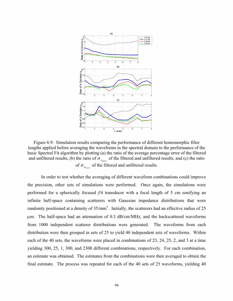
Figure 6.9: Simulation results comparing the performance of different homomorphic filter
lengths applied before averaging the waveforms in the spectral domain to the performance of the basic Spectral Fit algorithm by plotting (a) the ratio of the average percentage error of the filtered and unfiltered results, (b) the ratio of σ aupper
of the filtered and unfiltered results, and (c) the ratio of σ alower
of the filtered and unfiltered results.
In order to test whether the averaging of different waveform combinations could improve
the precision, other sets of simulations were performed. Once again, the simulations were
performed for a spherically focused f/4 transducer with a focal length of 5 cm sonifying an
infinite half-space containing scatterers with Gaussian impedance distributions that were
randomly positioned at a density of 35/mm3. Initially, the scatterers had an effective radius of 25
µm. The half-space had an attenuation of 0.3 dB/cm/MHz, and the backscattered waveforms
from 1000 independent scatterer distributions were generated. The waveforms from each
distribution were then grouped in sets of 25 to yield 40 independent sets of waveforms. Within
each of the 40 sets, the waveforms were placed in combinations of 23, 24, 25, 2, and 3 at a time
yielding 300, 25, 1, 300, and 2300 different combinations, respectively. For each combination,
an estimate was obtained. The estimates from the combinations were then averaged to obtain the
final estimate. The process was repeated for each of the 40 sets of 25 waveforms, yielding 40
94
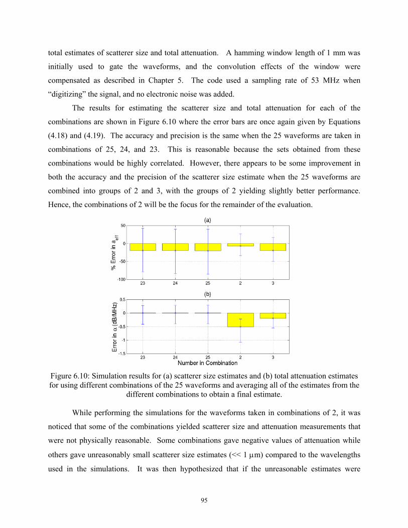
total estimates of scatterer size and total attenuation. A hamming window length of 1 mm was
initially used to gate the waveforms, and the convolution effects of the window were
compensated as described in Chapter 5. The code used a sampling rate of 53 MHz when
“digitizing” the signal, and no electronic noise was added.
The results for estimating the scatterer size and total attenuation for each of the
combinations are shown in Figure 6.10 where the error bars are once again given by Equations
(4.18) and (4.19). The accuracy and precision is the same when the 25 waveforms are taken in
combinations of 25, 24, and 23. This is reasonable because the sets obtained from these
combinations would be highly correlated. However, there appears to be some improvement in
both the accuracy and the precision of the scatterer size estimate when the 25 waveforms are
combined into groups of 2 and 3, with the groups of 2 yielding slightly better performance.
Hence, the combinations of 2 will be the focus for the remainder of the evaluation.
Figure 6.10: Simulation results for (a) scatterer size estimates and (b) total attenuation estimates for using different combinations of the 25 waveforms and averaging all of the estimates from the
different combinations to obtain a final estimate.
While performing the simulations for the waveforms taken in combinations of 2, it was
noticed that some of the combinations yielded scatterer size and attenuation measurements that
were not physically reasonable. Some combinations gave negative values of attenuation while
others gave unreasonably small scatterer size estimates (<< 1 µm) compared to the wavelengths
used in the simulations. It was then hypothesized that if the unreasonable estimates were
95
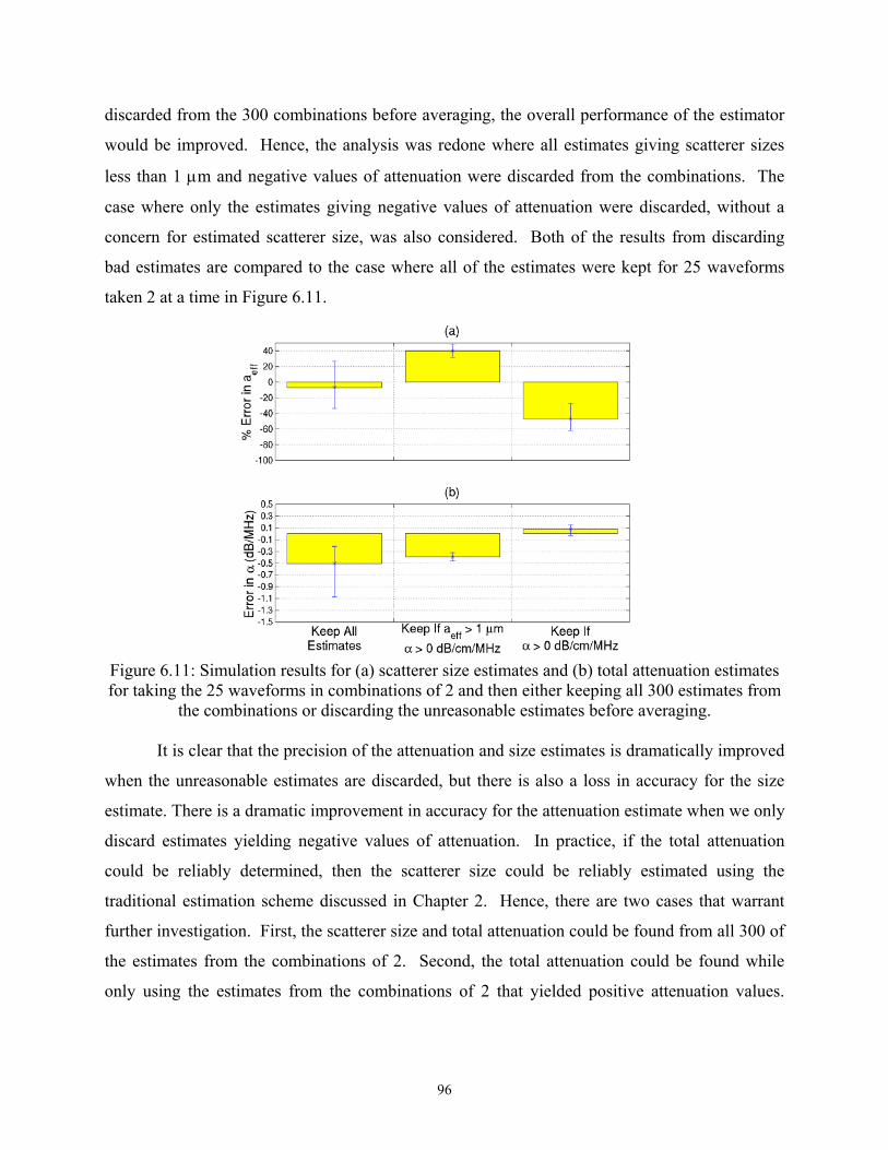
discarded from the 300 combinations before averaging, the overall performance of the estimator
would be improved. Hence, the analysis was redone where all estimates giving scatterer sizes
less than 1 µm and negative values of attenuation were discarded from the combinations. The
case where only the estimates giving negative values of attenuation were discarded, without a
concern for estimated scatterer size, was also considered. Both of the results from discarding
bad estimates are compared to the case where all of the estimates were kept for 25 waveforms
taken 2 at a time in Figure 6.11.
Figure 6.11: Simulation results for (a) scatterer size estimates and (b) total attenuation estimates for taking the 25 waveforms in combinations of 2 and then either keeping all 300 estimates from
the combinations or discarding the unreasonable estimates before averaging.
It is clear that the precision of the attenuation and size estimates is dramatically improved
when the unreasonable estimates are discarded, but there is also a loss in accuracy for the size
estimate. There is a dramatic improvement in accuracy for the attenuation estimate when we only
discard estimates yielding negative values of attenuation. In practice, if the total attenuation
could be reliably determined, then the scatterer size could be reliably estimated using the
traditional estimation scheme discussed in Chapter 2. Hence, there are two cases that warrant
further investigation. First, the scatterer size and total attenuation could be found from all 300 of
the estimates from the combinations of 2. Second, the total attenuation could be found while
only using the estimates from the combinations of 2 that yielded positive attenuation values.
96
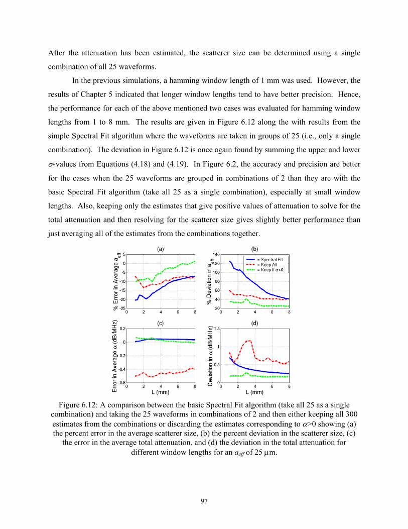
After the attenuation has been estimated, the scatterer size can be determined using a single
combination of all 25 waveforms.
In the previous simulations, a hamming window length of 1 mm was used. However, the
results of Chapter 5 indicated that longer window lengths tend to have better precision. Hence,
the performance for each of the above mentioned two cases was evaluated for hamming window
lengths from 1 to 8 mm. The results are given in Figure 6.12 along the with results from the
simple Spectral Fit algorithm where the waveforms are taken in groups of 25 (i.e., only a single
combination). The deviation in Figure 6.12 is once again found by summing the upper and lower
σ-values from Equations (4.18) and (4.19). In Figure 6.2, the accuracy and precision are better
for the cases when the 25 waveforms are grouped in combinations of 2 than they are with the
basic Spectral Fit algorithm (take all 25 as a single combination), especially at small window
lengths. Also, keeping only the estimates that give positive values of attenuation to solve for the
total attenuation and then resolving for the scatterer size gives slightly better performance than
just averaging all of the estimates from the combinations together.
Figure 6.12: A comparison between the basic Spectral Fit algorithm (take all 25 as a single
combination) and taking the 25 waveforms in combinations of 2 and then either keeping all 300 estimates from the combinations or discarding the estimates corresponding to α>0 showing (a) the percent error in the average scatterer size, (b) the percent deviation in the scatterer size, (c)
the error in the average total attenuation, and (d) the deviation in the total attenuation for different window lengths for an aeff of 25 µm.
97
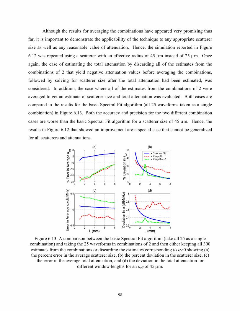
Although the results for averaging the combinations have appeared very promising thus
far, it is important to demonstrate the applicability of the technique to any appropriate scatterer
size as well as any reasonable value of attenuation. Hence, the simulation reported in Figure
6.12 was repeated using a scatterer with an effective radius of 45 µm instead of 25 µm. Once
again, the case of estimating the total attenuation by discarding all of the estimates from the
combinations of 2 that yield negative attenuation values before averaging the combinations,
followed by solving for scatterer size after the total attenuation had been estimated, was
considered. In addition, the case where all of the estimates from the combinations of 2 were
averaged to get an estimate of scatterer size and total attenuation was evaluated. Both cases are
compared to the results for the basic Spectral Fit algorithm (all 25 waveforms taken as a single
combination) in Figure 6.13. Both the accuracy and precision for the two different combination
cases are worse than the basic Spectral Fit algorithm for a scatterer size of 45 µm. Hence, the
results in Figure 6.12 that showed an improvement are a special case that cannot be generalized
for all scatterers and attenuations.
Figure 6.13: A comparison between the basic Spectral Fit algorithm (take all 25 as a single
combination) and taking the 25 waveforms in combinations of 2 and then either keeping all 300 estimates from the combinations or discarding the estimates corresponding to α>0 showing (a) the percent error in the average scatterer size, (b) the percent deviation in the scatterer size, (c)
the error in the average total attenuation, and (d) the deviation in the total attenuation for different window lengths for an aeff of 45 µm.
98
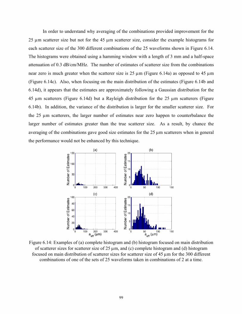
In order to understand why averaging of the combinations provided improvement for the
25 µm scatterer size but not for the 45 µm scatterer size, consider the example histograms for
each scatterer size of the 300 different combinations of the 25 waveforms shown in Figure 6.14.
The histograms were obtained using a hamming window with a length of 3 mm and a half-space
attenuation of 0.3 dB/cm/MHz. The number of estimates of scatterer size from the combinations
near zero is much greater when the scatterer size is 25 µm (Figure 6.14a) as opposed to 45 µm
(Figure 6.14c). Also, when focusing on the main distribution of the estimates (Figure 6.14b and
6.14d), it appears that the estimates are approximately following a Gaussian distribution for the
45 µm scatterers (Figure 6.14d) but a Rayleigh distribution for the 25 µm scatterers (Figure
6.14b). In addition, the variance of the distribution is larger for the smaller scatterer size. For
the 25 µm scatterers, the larger number of estimates near zero happen to counterbalance the
larger number of estimates greater than the true scatterer size. As a result, by chance the
averaging of the combinations gave good size estimates for the 25 µm scatterers when in general
the performance would not be enhanced by this technique.
Figure 6.14: Examples of (a) complete histogram and (b) histogram focused on main distribution
of scatterer sizes for scatterer size of 25 µm, and (c) complete histogram and (d) histogram focused on main distribution of scatterer sizes for scatterer size of 45 µm for the 300 different
combinations of one of the sets of 25 waveforms taken in combinations of 2 at a time.
99
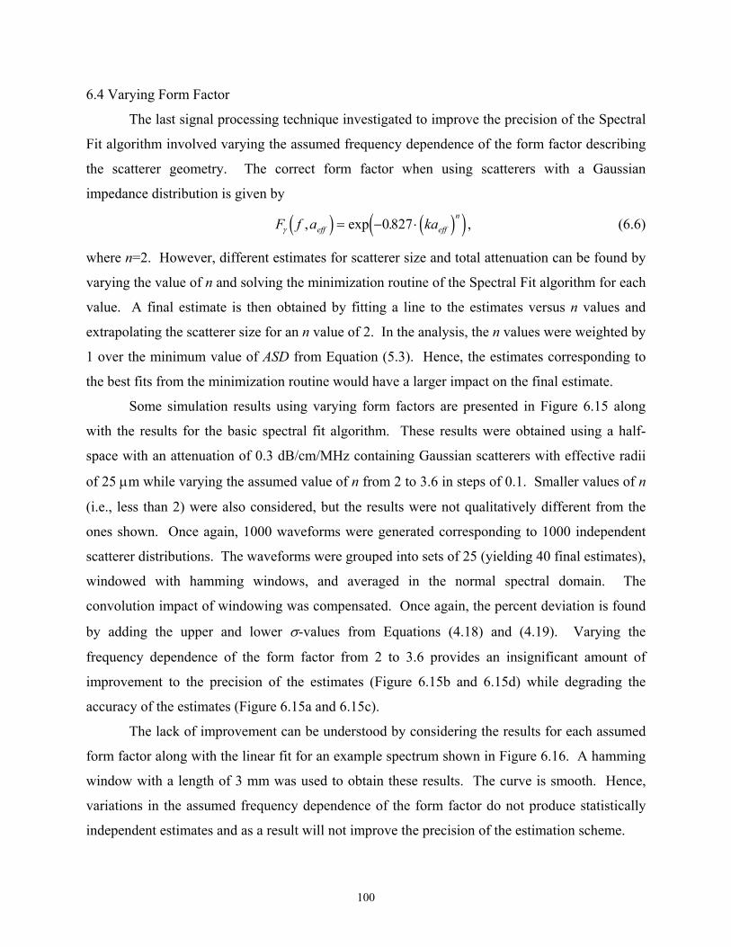
6.4 Varying Form Factor
The last signal processing technique investigated to improve the precision of the Spectral
Fit algorithm involved varying the assumed frequency dependence of the form factor describing
the scatterer geometry. The correct form factor when using scatterers with a Gaussian
impedance distribution is given by
F f a kaeff eff
n
γ , exp .d i d ie j= − ⋅0 827 , (6.6)
where n=2. However, different estimates for scatterer size and total attenuation can be found by
varying the value of n and solving the minimization routine of the Spectral Fit algorithm for each
value. A final estimate is then obtained by fitting a line to the estimates versus n values and
extrapolating the scatterer size for an n value of 2. In the analysis, the n values were weighted by
1 over the minimum value of ASD from Equation (5.3). Hence, the estimates corresponding to
the best fits from the minimization routine would have a larger impact on the final estimate.
Some simulation results using varying form factors are presented in Figure 6.15 along
with the results for the basic spectral fit algorithm. These results were obtained using a half-
space with an attenuation of 0.3 dB/cm/MHz containing Gaussian scatterers with effective radii
of 25 µm while varying the assumed value of n from 2 to 3.6 in steps of 0.1. Smaller values of n
(i.e., less than 2) were also considered, but the results were not qualitatively different from the
ones shown. Once again, 1000 waveforms were generated corresponding to 1000 independent
scatterer distributions. The waveforms were grouped into sets of 25 (yielding 40 final estimates),
windowed with hamming windows, and averaged in the normal spectral domain. The
convolution impact of windowing was compensated. Once again, the percent deviation is found
by adding the upper and lower σ-values from Equations (4.18) and (4.19). Varying the
frequency dependence of the form factor from 2 to 3.6 provides an insignificant amount of
improvement to the precision of the estimates (Figure 6.15b and 6.15d) while degrading the
accuracy of the estimates (Figure 6.15a and 6.15c).
The lack of improvement can be understood by considering the results for each assumed
form factor along with the linear fit for an example spectrum shown in Figure 6.16. A hamming
window with a length of 3 mm was used to obtain these results. The curve is smooth. Hence,
variations in the assumed frequency dependence of the form factor do not produce statistically
independent estimates and as a result will not improve the precision of the estimation scheme.
100
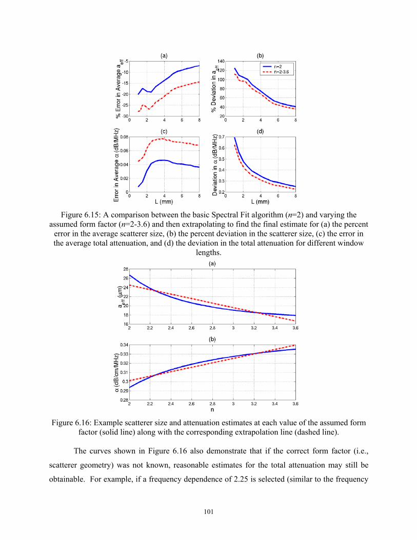
Figure 6.15: A comparison between the basic Spectral Fit algorithm (n=2) and varying the
assumed form factor (n=2-3.6) and then extrapolating to find the final estimate for (a) the percent error in the average scatterer size, (b) the percent deviation in the scatterer size, (c) the error in the average total attenuation, and (d) the deviation in the total attenuation for different window
lengths.
Figure 6.16: Example scatterer size and attenuation estimates at each value of the assumed form
factor (solid line) along with the corresponding extrapolation line (dashed line).
The curves shown in Figure 6.16 also demonstrate that if the correct form factor (i.e.,
scatterer geometry) was not known, reasonable estimates for the total attenuation may still be
obtainable. For example, if a frequency dependence of 2.25 is selected (similar to the frequency
101
102
dependence of a spherical shell type scatterer over some frequency bandwidths), then the
estimated attenuation value will differ by only about 0.01 dB/cm/MHz from the value given for
the true frequency dependence of 2. Unfortunately, the scatterer size will still vary with the
form factor because the constant term (i.e., 0.827 for Gaussian scatterers) will vary depending
upon the scatterer geometry. However, applications such as acoustic radiation force impulse
imaging and thermal dose predicting, which only require the attenuation and not the scatterer
size, would still benefit from the estimation scheme based on these results even when the correct
form factor is not known. This conclusion is important because the correct form factor for
biological tissue remains to be determined.
6.5 Chapter Summary
In this chapter, four different signal processing strategies were investigated with the hope
of improving the precision of the Spectral Fit algorithm. The first averaged together estimates
from different window lengths, but the precision was not improved. The second strategy
involved using homomorphic signal processing to smooth the spectra before the fit.
Homomorphic signal processing did not improve the precision, nor did it reduce the number of
RF echoes required to achieve the same level of precision. The third strategy involved taking the
RF echoes in different combinations and then averaging the results together. The strategy
worked well for 25 µm scatterers by coincidence, but the algorithm had poor accuracy at other
scatterer sizes. The last strategy involved varying the frequency dependence of the form factor,
obtaining estimates at each assumed form factor, and then extrapolating to find the estimate at
the true form factor. Once again, there was no improvement in the precision due to the
correlation between estimates with only slightly different form factors. However, this also
means that it may be possible to obtain accurate attenuation estimates when the correct form
factor is not known.
CHAPTER 7
EFFECT OF kaeff VALUES AND FREQUENCY RANGE USED IN ESTIMATION
While performing the analysis of the different signal processing techniques discussed in
Chapter 6, it was noted that the precision of estimates from the basic Spectral Fit algorithm were
better for the larger scatterer size of 45 µm. For example, the smallest percent deviation of
scatterer size (precision) in Figure 6.12 is ~40% for the 25 µm scatterers, whereas the percent
deviation at the same window length in Figure 6.13 is ~15% for the 45 µm scatterers. This calls
into question the previous choice of kaeff values that attempted to center the bandwidth near a
kaeff value of 0.8 (i.e., a frequency of 8 MHz for a scatterer size of 25 µm). Initially, this kaeff
value had been selected because the optimal range for kaeff values had been previously reported
as being from 0.5 to 1.2 [Insana and Hall, 1990]. Hence, in this chapter the impact the choice of
kaeff values has on the estimation scheme is analyzed. The analysis is done for both the Spectral
Fit algorithm that estimates both scatterer size and total attenuation as well as for the traditional
minimization algorithm that assumes the attenuation is already known. The analysis only
considers scatterers with Gaussian impedance distributions.
7.1 kaeff Range Results for the Spectral Fit Algorithm
In order to evaluate the impact the kaeff values have on the Spectral Fit algorithm, many
different sets of simulations were performed. In the simulations, a weakly focused f/4 transducer
with a focal length of 5 cm was once again used to sonify an infinite half-space with scatterers
placed at a density of 35/mm3. Also, 1000 independent scatterer distributions were used for each
of the simulated cases, and a waveform was generated for each distribution. A sampling
frequency of 53 MHz was used when “digitizing” each of the waveforms. The resulting 1000
independent waveforms were combined into 40 sets with 25 waveforms per set. The 25
waveforms in each set were windowed with a hamming window whose length varied from 1 to 8
103

mm and averaged in the normal spectral domain. The averaged spectrum was then compensated
for windowing and used in the Spectral Fit algorithm to obtain an estimate for total attenuation α
and effective scatterer size aeff. The effect of using different kaeff ranges was evaluated by
varying the attenuation of the half-space, the scatterer size, the bandwidth of the source, and the
amount of electronic noise added to the simulated waveforms before processing.
7.1.1 Results for different source bandwidths
The first case that will be analyzed involved varying the bandwidth of the source and the
scatterer size while maintaining the same value for the half-space attenuation. In order to
facilitate the analysis, the attenuation selected for the half-space was 0 dB/cm/MHz, so that the
attenuation would not cause any downshift in the backscattered spectrum. However, the Spectral
Fit algorithm still solved for the attenuation as if it was unknown. The bandwidth of the source
was varied by changing the bandwidth of the Rayleigh distribution of the filtering characteristics
for the source (i.e., H(f)). In the simulations, H(f) was given by
H f
f f f
f f f
R
R
f
R
R
b g =⋅ −
−FHG
IKJ
FHG
IKJ
⋅ −−FHG
IKJ
FHG
IKJ
FHGG
IKJJ∀
exp
max exp
σ
σ
2
2, (7.1)
where fR was 8 MHz and σR was varied as 2, 4, and 6 MHz in order to change the bandwidth of
the source. Then, the frequency range (i.e., range of kaeff values) used in the minimization
routine was given by the set of all frequencies corresponding to signal levels greater than
NP f f
P fFloor
scat N N
f scat Gaussianfit
= − FHG
IKJ
F
H
GGGG
I
K
JJJJ
F
H
GGGG
I
K
JJJJ+
L
N
MMMMM
O
Q
PPPPP
F
H
GGGGG
I
K
JJJJJ
−
∀
max mean log:
max20 10 6200b g
b gm r (7.2)
as was discussed in Chapter 5. For each source bandwidth, simulations were performed with
scatterer effective radii varying from 5 to 105 µm. However, within each simulation, every
scatterer had the same size.
The results at each bandwidth for a window length of 3 mm for all of the scatterer sizes
are shown in Figure 7.1. There is a significant degradation in both accuracy and precision for the
104
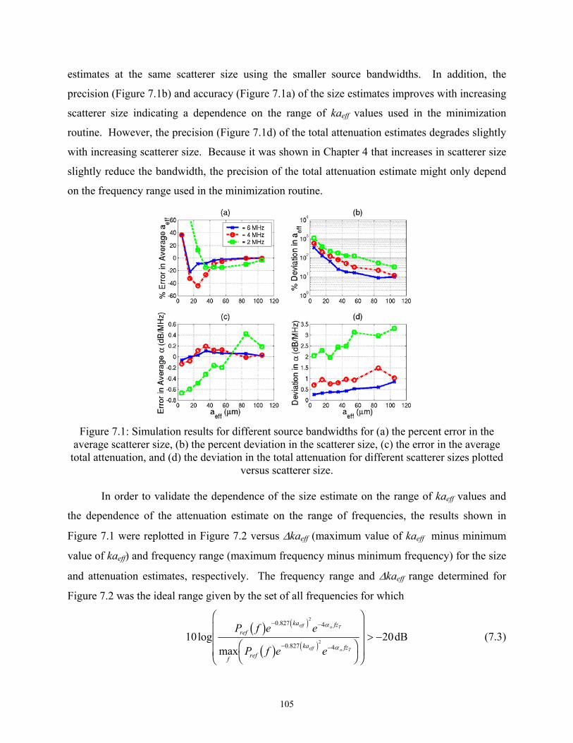
estimates at the same scatterer size using the smaller source bandwidths. In addition, the
precision (Figure 7.1b) and accuracy (Figure 7.1a) of the size estimates improves with increasing
scatterer size indicating a dependence on the range of kaeff values used in the minimization
routine. However, the precision (Figure 7.1d) of the total attenuation estimates degrades slightly
with increasing scatterer size. Because it was shown in Chapter 4 that increases in scatterer size
slightly reduce the bandwidth, the precision of the total attenuation estimate might only depend
on the frequency range used in the minimization routine.
Figure 7.1: Simulation results for different source bandwidths for (a) the percent error in the
average scatterer size, (b) the percent deviation in the scatterer size, (c) the error in the average total attenuation, and (d) the deviation in the total attenuation for different scatterer sizes plotted
versus scatterer size.
In order to validate the dependence of the size estimate on the range of kaeff values and
the dependence of the attenuation estimate on the range of frequencies, the results shown in
Figure 7.1 were replotted in Figure 7.2 versus ∆kaeff (maximum value of kaeff minus minimum
value of kaeff) and frequency range (maximum frequency minus minimum frequency) for the size
and attenuation estimates, respectively. The frequency range and ∆kaeff range determined for
Figure 7.2 was the ideal range given by the set of all frequencies for which
10 200 827 4
0 827 4
2
2logmax
dB.
.
P f e e
P f e e
refka fz
f refka fz
eff o T
eff o T
b gb g
d i
d i
− −
− −FH
IK
F
HGGG
I
KJJJ> −
α
α (7.3)
105

because for these simulated cases no noise had been added to the waveforms. Clearly from
Figure 7.2, the accuracy (Figure 7.2a) and precision (Figure 7.2b) of the size estimates exhibit a
strong and consistent dependence on ∆kaeff as is indicated by the overlapping curves. Likewise,
the accuracy (Figure 7.2c) and precision (Figure 7.2d) of the attenuation estimates exhibit a
strong dependence on the frequency range used in the minimization. However, the relationship
between the accuracy of the attenuation estimates and the frequency range used by the
minimization is not as consistent (i.e., curves do not overlap) as the other cases shown in Figure
7.2.
Figure 7.2: Simulation results for different source bandwidths for (a) the percent error in the
average scatterer size, (b) the percent deviation in the scatterer size, (c) the error in the average total attenuation, and (d) the deviation in the total attenuation for different scatterer sizes plotted
versus ∆kaeff and frequency range used in minimization.
7.1.2 Results for different half-space attenuations
After showing that the accuracy and precision of the estimates were dependent on ∆kaeff
and the frequency range used when varying the bandwidth of the source, changes in the ∆kaeff
and the frequency range were investigated to determine if they could also explain the previously
observed loss in precision with increasing attenuation (Chapter 5). Hence, simulations were
performed for half-space attenuation of 0.3 dB/cm/MHz, 0.5 dB/cm/MHz, and 1 dB/cm/MHz.
For each value of half-space attenuation, the bandwidth of the source was held constant and set
by using a σR value of 6 MHz in Equation (7.1). The frequency range used in the minimization
106
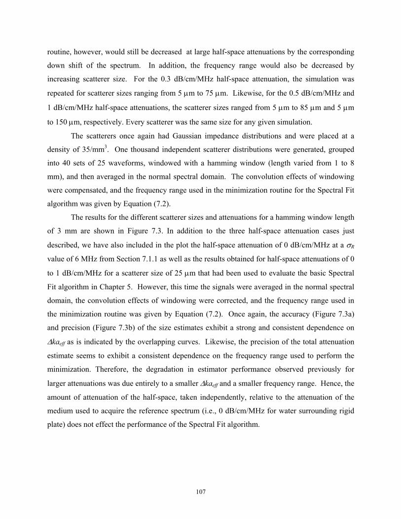
routine, however, would still be decreased at large half-space attenuations by the corresponding
down shift of the spectrum. In addition, the frequency range would also be decreased by
increasing scatterer size. For the 0.3 dB/cm/MHz half-space attenuation, the simulation was
repeated for scatterer sizes ranging from 5 µm to 75 µm. Likewise, for the 0.5 dB/cm/MHz and
1 dB/cm/MHz half-space attenuations, the scatterer sizes ranged from 5 µm to 85 µm and 5 µm
to 150 µm, respectively. Every scatterer was the same size for any given simulation.
The scatterers once again had Gaussian impedance distributions and were placed at a
density of 35/mm3. One thousand independent scatterer distributions were generated, grouped
into 40 sets of 25 waveforms, windowed with a hamming window (length varied from 1 to 8
mm), and then averaged in the normal spectral domain. The convolution effects of windowing
were compensated, and the frequency range used in the minimization routine for the Spectral Fit
algorithm was given by Equation (7.2).
The results for the different scatterer sizes and attenuations for a hamming window length
of 3 mm are shown in Figure 7.3. In addition to the three half-space attenuation cases just
described, we have also included in the plot the half-space attenuation of 0 dB/cm/MHz at a σR
value of 6 MHz from Section 7.1.1 as well as the results obtained for half-space attenuations of 0
to 1 dB/cm/MHz for a scatterer size of 25 µm that had been used to evaluate the basic Spectral
Fit algorithm in Chapter 5. However, this time the signals were averaged in the normal spectral
domain, the convolution effects of windowing were corrected, and the frequency range used in
the minimization routine was given by Equation (7.2). Once again, the accuracy (Figure 7.3a)
and precision (Figure 7.3b) of the size estimates exhibit a strong and consistent dependence on
∆kaeff as is indicated by the overlapping curves. Likewise, the precision of the total attenuation
estimate seems to exhibit a consistent dependence on the frequency range used to perform the
minimization. Therefore, the degradation in estimator performance observed previously for
larger attenuations was due entirely to a smaller ∆kaeff and a smaller frequency range. Hence, the
amount of attenuation of the half-space, taken independently, relative to the attenuation of the
medium used to acquire the reference spectrum (i.e., 0 dB/cm/MHz for water surrounding rigid
plate) does not effect the performance of the Spectral Fit algorithm.
107

Figure 7.3: Simulation results for different half-space attenuations for (a) the percent error in the average scatterer size, (b) the percent deviation in the scatterer size, (c) the error in the average
total attenuation, and (d) the deviation in the total attenuation plotted versus ∆kaeff and the frequency range used in minimization.
To further demonstrate the lack of dependence of the algorithm on the attenuation of the
half-space relative to the reference medium, a new reference waveform was acquired. This time,
the attenuation of the medium between the source and reference plate placed at the focal plane
was changed from 0 dB/cm/MHz (water) to 0.3 dB/cm/MHz. The new reference waveform was
then used in the Spectral Fit algorithm to estimate total attenuation and scatterer size for a half-
space with an attenuation of 0.3 dB/cm/MHz containing Gaussian scatterers with radii of 25 µm.
The results for both the lossless (water) and lossy reference waveforms for this case are shown in
Figure 7.4. The results for the two different reference waveforms are identical confirming that
attenuation of the half-space relative to the reference does not matter.
7.1.3 Results for different levels of electronic noise
In Chapter 5, the performance of the Spectral Fit algorithm was also degraded by adding
white “electronic” noise to the simulated waveforms in addition to the degradation observed by
increasing the attenuation of the half-space. Hence, after completing the investigation on the
impact of attenuation discussed in Section 7.1.2, the impact of adding white, Gaussian
distributed, noise to the acquired waveforms was investigated. The waveforms selected for the
108
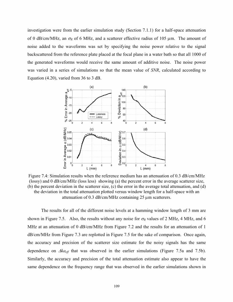
investigation were from the earlier simulation study (Section 7.1.1) for a half-space attenuation
of 0 dB/cm/MHz, an σR of 6 MHz, and a scatterer effective radius of 105 µm. The amount of
noise added to the waveforms was set by specifying the noise power relative to the signal
backscattered from the reference plate placed at the focal plane in a water bath so that all 1000 of
the generated waveforms would receive the same amount of additive noise. The noise power
was varied in a series of simulations so that the mean value of SNR, calculated according to
Equation (4.20), varied from 36 to 3 dB.
Figure 7.4: Simulation results when the reference medium has an attenuation of 0.3 dB/cm/MHz (lossy) and 0 dB/cm/MHz (loss less) showing (a) the percent error in the average scatterer size,
(b) the percent deviation in the scatterer size, (c) the error in the average total attenuation, and (d) the deviation in the total attenuation plotted versus window length for a half-space with an
attenuation of 0.3 dB/cm/MHz containing 25 µm scatterers.
The results for all of the different noise levels at a hamming window length of 3 mm are
shown in Figure 7.5. Also, the results without any noise for σR values of 2 MHz, 4 MHz, and 6
MHz at an attenuation of 0 dB/cm/MHz from Figure 7.2 and the results for an attenuation of 1
dB/cm/MHz from Figure 7.3 are replotted in Figure 7.5 for the sake of comparison. Once again,
the accuracy and precision of the scatterer size estimate for the noisy signals has the same
dependence on ∆kaeff that was observed in the earlier simulations (Figure 7.5a and 7.5b).
Similarly, the accuracy and precision of the total attenuation estimate also appear to have the
same dependence on the frequency range that was observed in the earlier simulations shown in
109
Figure 7.2 that varied the value of σR. However, the precision of the attenuation estimate for the
half-space attenuation of 1 dB/cm/MHz at smaller frequency ranges (i.e., less than 6 MHz)
appears to be better than that expected by the other simulations. This difference was not noticed
previously because of the gap in data for the frequency range from 4 to 6 MHz. From this we
can conclude that although the accuracy and precision of the attenuation estimate are improved
with increasing frequency range used to obtain the estimate, the exact amount of improvement
may be difficult to predict from the frequency range alone.
Figure 7.5: Simulation results for different levels of electronic noise for (a) the percent error in
the average scatterer size, (b) the percent deviation in the scatterer size, (c) the error in the average total attenuation, and (d) the deviation in the total attenuation plotted along with results for different bandwidth sources and a half-space attenuation of 1 dB/cm/MHz versus ∆kaeff and
the frequency range used in minimization.
7.2 kaeff Range Results for the Traditional Algorithm
In the previous section, it was observed that the accuracy and precision of the size
estimates were improved as we increased the size of the ∆kaeff range used in the minimization
routine. In this section, the traditional estimation scheme where the attenuation is known a
priori was investigated to determine if the same trend in improvement was also found. The
relationship between frequency range and precision of the size estimate using the traditional
estimation scheme has been investigated briefly by other authors [Chaturvedi and Insana, 1996;
Wear, 2001b]. However, in their analysis they only looked at the impact of frequency range and
not the ∆kaeff range. In addition, although Chaturvedi and Insana’s results for two different
110

scatterer sizes suggest a consistent dependence of precision on the ∆kaeff range, the results were
not presented in a form to facilitate a comparison. Hence, the comparison was performed using
new simulation results.
Before performing the comparison, however, the initial kaeff values used in the estimate
were investigated to determine if they should be greater than 0.5 as had been previously reported
[Insana and Hall, 1990]. Hence, simulations were performed where the ∆kaeff range was set to
be one, and the initial kaeff value was varied from 0.1 to 2. The frequency range used in the
minimization was manually selected for these simulations, but care was still taken to insure that
the selected frequencies corresponded to signal values greater than the noise floor of the
simulated waveforms. The half-space used in the simulations had an attenuation of 0
dB/cm/MHz and once again contained Gaussian scatterers with an aeff of 25 µm at a density of
35/mm3. The sources used in the simulations had very large bandwidths that would not be
physically realizable with a real source so that the large span of kaeff values could be tested. The
bandwidth was set by using a filtering function given by
H f
f f
f ff
b ge je j
e je j=
− − ⋅ −FHGIKJ
FHG
IKJ
− − ⋅ −FHGIKJ
FHG
IKJ
FHG
IKJ
−
∀
−
1 620
1 620
12
12
exp MHz expMHz
max exp MHz expMHz
(7.4)
while still shock exciting the simulated transducers (i.e., Vinc(ω)=1). Three different sources
were used in the simulations with f-numbers of 1, 2, and 4. The effects of focusing and
attenuation were removed using the generalized attenuation-compensation function discussed in
Chapter 2.
Once again, 1000 backscattered waveforms for 1000 independent scatterer distributions
were generated and combined into 40 sets with 25 waveforms per set for each source. However,
the sampling rate selected when “digitizing” the signal for the simulated waveforms was 125
MHz, not the 53 MHz used previously, in order to accommodate the large bandwidth of the
transducer. Also, no “electronic” noise was added to the simulated waveforms. The 25
waveforms in each set were windowed with a hamming window of length 3 mm. The averaged
spectrum was then compensated for windowing using the same compensation technique that was
described in Chapter 5 for the Spectral Fit Algorithm.
111
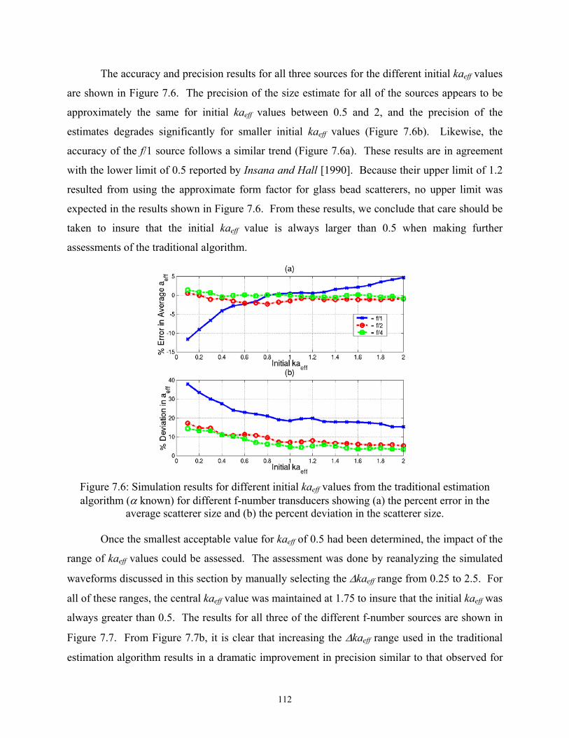
The accuracy and precision results for all three sources for the different initial kaeff values
are shown in Figure 7.6. The precision of the size estimate for all of the sources appears to be
approximately the same for initial kaeff values between 0.5 and 2, and the precision of the
estimates degrades significantly for smaller initial kaeff values (Figure 7.6b). Likewise, the
accuracy of the f/1 source follows a similar trend (Figure 7.6a). These results are in agreement
with the lower limit of 0.5 reported by Insana and Hall [1990]. Because their upper limit of 1.2
resulted from using the approximate form factor for glass bead scatterers, no upper limit was
expected in the results shown in Figure 7.6. From these results, we conclude that care should be
taken to insure that the initial kaeff value is always larger than 0.5 when making further
assessments of the traditional algorithm.
Figure 7.6: Simulation results for different initial kaeff values from the traditional estimation algorithm (α known) for different f-number transducers showing (a) the percent error in the
average scatterer size and (b) the percent deviation in the scatterer size.
Once the smallest acceptable value for kaeff of 0.5 had been determined, the impact of the
range of kaeff values could be assessed. The assessment was done by reanalyzing the simulated
waveforms discussed in this section by manually selecting the ∆kaeff range from 0.25 to 2.5. For
all of these ranges, the central kaeff value was maintained at 1.75 to insure that the initial kaeff was
always greater than 0.5. The results for all three of the different f-number sources are shown in
Figure 7.7. From Figure 7.7b, it is clear that increasing the ∆kaeff range used in the traditional
estimation algorithm results in a dramatic improvement in precision similar to that observed for
112
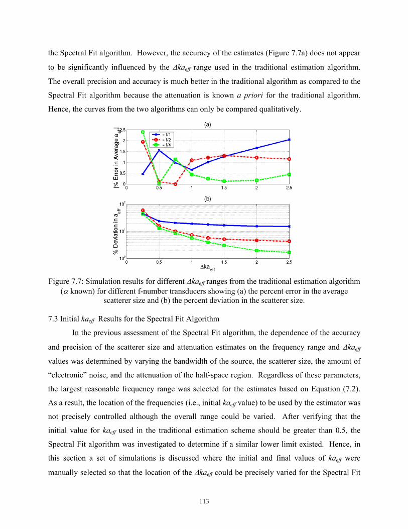
the Spectral Fit algorithm. However, the accuracy of the estimates (Figure 7.7a) does not appear
to be significantly influenced by the ∆kaeff range used in the traditional estimation algorithm.
The overall precision and accuracy is much better in the traditional algorithm as compared to the
Spectral Fit algorithm because the attenuation is known a priori for the traditional algorithm.
Hence, the curves from the two algorithms can only be compared qualitatively.
Figure 7.7: Simulation results for different ∆kaeff ranges from the traditional estimation algorithm
(α known) for different f-number transducers showing (a) the percent error in the average scatterer size and (b) the percent deviation in the scatterer size.
7.3 Initial kaeff Results for the Spectral Fit Algorithm
In the previous assessment of the Spectral Fit algorithm, the dependence of the accuracy
and precision of the scatterer size and attenuation estimates on the frequency range and ∆kaeff
values was determined by varying the bandwidth of the source, the scatterer size, the amount of
“electronic” noise, and the attenuation of the half-space region. Regardless of these parameters,
the largest reasonable frequency range was selected for the estimates based on Equation (7.2).
As a result, the location of the frequencies (i.e., initial kaeff value) to be used by the estimator was
not precisely controlled although the overall range could be varied. After verifying that the
initial value for kaeff used in the traditional estimation scheme should be greater than 0.5, the
Spectral Fit algorithm was investigated to determine if a similar lower limit existed. Hence, in
this section a set of simulations is discussed where the initial and final values of kaeff were
manually selected so that the location of the ∆kaeff could be precisely varied for the Spectral Fit
113
algorithm. However, care was still taken to insure that the frequency range used in the
minimization did not extend into spectral regions dominated by noise.
In order to vary the location of the ∆kaeff while still maintaining a ∆kaeff that would yield
reasonable accuracy and precision, an ultrasound source with a very large frequency bandwidth
was desired. Hence, simulations were performed using a source with a σR of 18 MHz and a fR of
8 MHz in the filtering function given by Equation (7.1). It is not possible using current
technology to obtain a real source with this large a bandwidth. However, a bandwidth of this
duration was required for the analysis. The source had an f-number of 4 and a 5 cm focal length
as well.
The idealized source sonified a half-space containing scatterers with Gaussian impedance
distributions with effective radii of 25 µm at a density of 35/mm3. The half-space had an
attenuation of 0 dB/cm/MHz. Once again, 1000 backscattered waveforms for 1000 independent
scatterer distributions were generated and combined into 40 sets with 25 waveforms per set.
However, the sampling rate selected when “digitizing” the signal for the simulated waveforms
was 160 MHz instead of the 53 MHz used previously in order to accommodate the large
bandwidth of the transducer. Also, no “electronic” noise was added to the simulated waveforms.
The 25 waveforms in each set were windowed with a hamming window with a length of 3 mm
and averaged in the normal spectral domain. The averaged spectrum was then compensated for
windowing and used in the Spectral Fit algorithm to obtain an estimate for total attenuation and
effective scatterer size.
In addition to the idealized source just described, the simulated f/4 data used previously
to assesses the impact of the kaeff values on the performance of the traditional algorithm (i.e.,
source filtering function given by Equation (7.4)) was also reanalyzed using the Spectral Fit
algorithm. For both idealized sources, ∆kaeff was set to one and the initial kaeff value was varied
over the largest possible range while still avoiding the sections of the spectrum dominated by
noise. Because the scatterer size, attenuation, frequency range used in the minimization, and
focal length for both of these simulated sources were identical, the accuracy and precision for
both idealized sources should have been the same. However, this was not the case as is shown in
Figure 7.8.
114
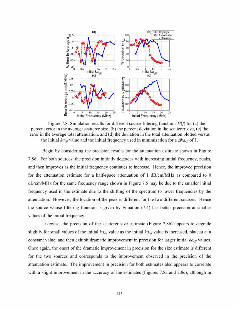
Figure 7.8: Simulation results for different source filtering functions H(f) for (a) the
percent error in the average scatterer size, (b) the percent deviation in the scatterer size, (c) the error in the average total attenuation, and (d) the deviation in the total attenuation plotted versus
the initial kaeff value and the initial frequency used in minimization for a ∆kaeff of 1.
Begin by considering the precision results for the attenuation estimate shown in Figure
7.8d. For both sources, the precision initially degrades with increasing initial frequency, peaks,
and then improves as the initial frequency continues to increase. Hence, the improved precision
for the attenuation estimate for a half-space attenuation of 1 dB/cm/MHz as compared to 0
dB/cm/MHz for the same frequency range shown in Figure 7.5 may be due to the smaller initial
frequency used in the estimate due to the shifting of the spectrum to lower frequencies by the
attenuation. However, the location of the peak is different for the two different sources. Hence
the source whose filtering function is given by Equation (7.4) has better precision at smaller
values of the initial frequency.
Likewise, the precision of the scatterer size estimate (Figure 7.8b) appears to degrade
slightly for small values of the initial kaeff value as the initial kaeff value is increased, plateau at a
constant value, and then exhibit dramatic improvement in precision for larger initial kaeff values.
Once again, the onset of the dramatic improvement in precision for the size estimate is different
for the two sources and corresponds to the improvement observed in the precision of the
attenuation estimate. The improvement in precision for both estimates also appears to correlate
with a slight improvement in the accuracy of the estimates (Figures 7.8a and 7.8c), although in
115
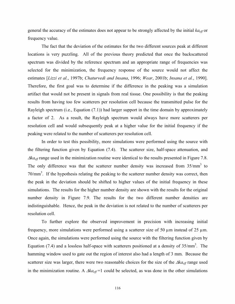
general the accuracy of the estimates does not appear to be strongly affected by the initial kaeff or
frequency value.
The fact that the deviation of the estimates for the two different sources peak at different
locations is very puzzling. All of the previous theory predicted that once the backscattered
spectrum was divided by the reference spectrum and an appropriate range of frequencies was
selected for the minimization, the frequency response of the source would not affect the
estimates [Lizzi et al., 1997b; Chaturvedi and Insana, 1996; Wear, 2001b; Insana et al., 1990].
Therefore, the first goal was to determine if the difference in the peaking was a simulation
artifact that would not be present in signals from real tissue. One possibility is that the peaking
results from having too few scatterers per resolution cell because the transmitted pulse for the
Rayleigh spectrum (i.e., Equation (7.1)) had larger support in the time domain by approximately
a factor of 2. As a result, the Rayleigh spectrum would always have more scatterers per
resolution cell and would subsequently peak at a higher value for the initial frequency if the
peaking were related to the number of scatterers per resolution cell.
In order to test this possibility, more simulations were performed using the source with
the filtering function given by Equation (7.4). The scatterer size, half-space attenuation, and
∆kaeff range used in the minimization routine were identical to the results presented in Figure 7.8.
The only difference was that the scatterer number density was increased from 35/mm3 to
70/mm3. If the hypothesis relating the peaking to the scatterer number density was correct, then
the peak in the deviation should be shifted to higher values of the initial frequency in these
simulations. The results for the higher number density are shown with the results for the original
number density in Figure 7.9. The results for the two different number densities are
indistinguishable. Hence, the peak in the deviation is not related to the number of scatterers per
resolution cell.
To further explore the observed improvement in precision with increasing initial
frequency, more simulations were performed using a scatterer size of 50 µm instead of 25 µm.
Once again, the simulations were performed using the source with the filtering function given by
Equation (7.4) and a lossless half-space with scatterers positioned at a density of 35/mm3. The
hamming window used to gate out the region of interest also had a length of 3 mm. Because the
scatterer size was larger, there were two reasonable choices for the size of the ∆kaeff range used
in the minimization routine. A ∆kaeff =1 could be selected, as was done in the other simulations
116
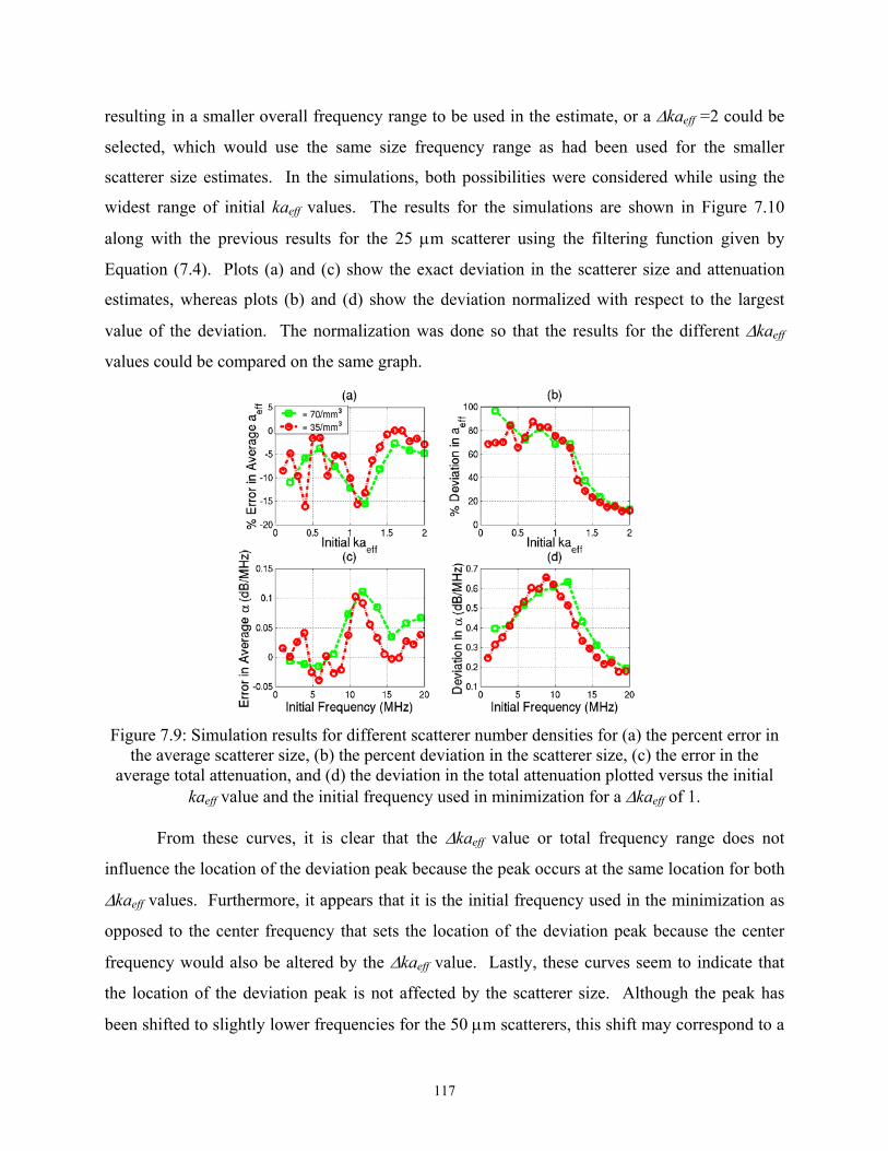
resulting in a smaller overall frequency range to be used in the estimate, or a ∆kaeff =2 could be
selected, which would use the same size frequency range as had been used for the smaller
scatterer size estimates. In the simulations, both possibilities were considered while using the
widest range of initial kaeff values. The results for the simulations are shown in Figure 7.10
along with the previous results for the 25 µm scatterer using the filtering function given by
Equation (7.4). Plots (a) and (c) show the exact deviation in the scatterer size and attenuation
estimates, whereas plots (b) and (d) show the deviation normalized with respect to the largest
value of the deviation. The normalization was done so that the results for the different ∆kaeff
values could be compared on the same graph.
Figure 7.9: Simulation results for different scatterer number densities for (a) the percent error in
the average scatterer size, (b) the percent deviation in the scatterer size, (c) the error in the average total attenuation, and (d) the deviation in the total attenuation plotted versus the initial
kaeff value and the initial frequency used in minimization for a ∆kaeff of 1.
From these curves, it is clear that the ∆kaeff value or total frequency range does not
influence the location of the deviation peak because the peak occurs at the same location for both
∆kaeff values. Furthermore, it appears that it is the initial frequency used in the minimization as
opposed to the center frequency that sets the location of the deviation peak because the center
frequency would also be altered by the ∆kaeff value. Lastly, these curves seem to indicate that
the location of the deviation peak is not affected by the scatterer size. Although the peak has
been shifted to slightly lower frequencies for the 50 µm scatterers, this shift may correspond to a
117
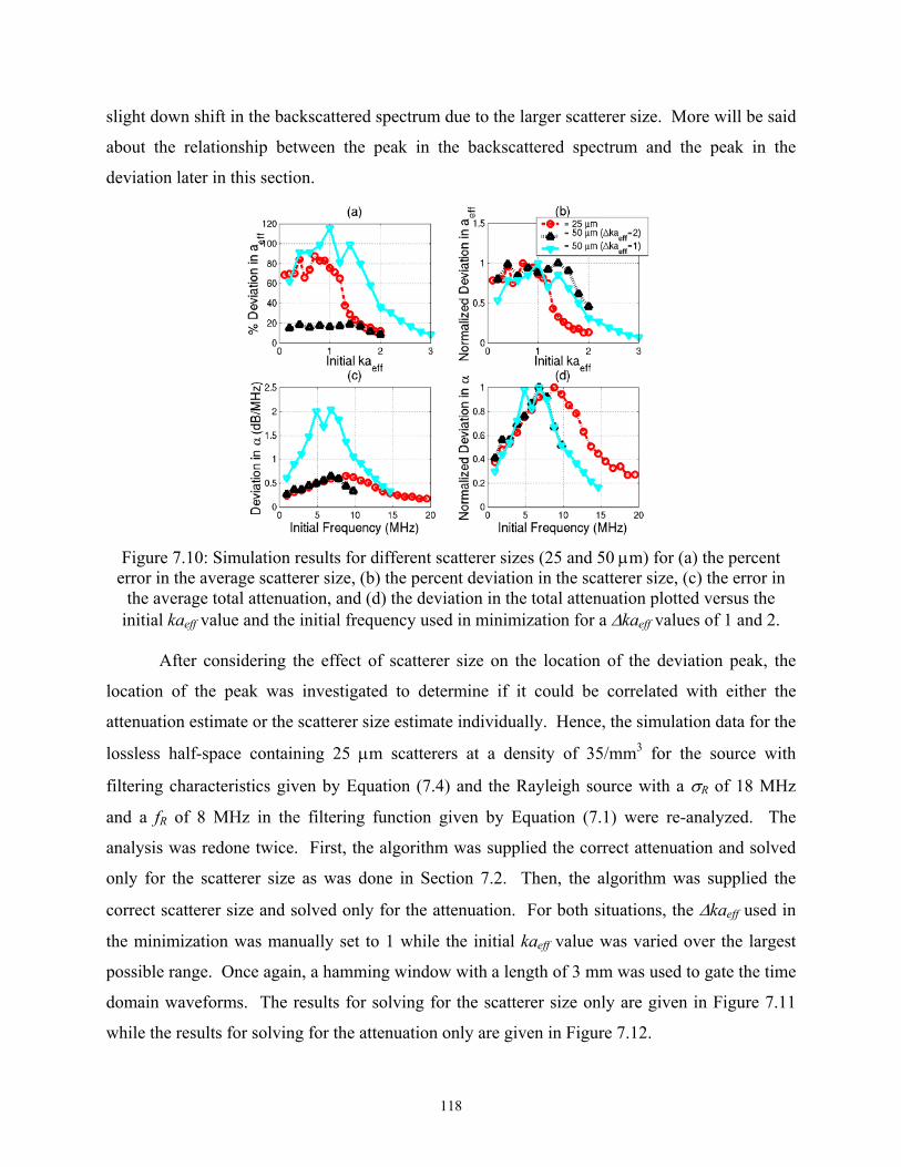
slight down shift in the backscattered spectrum due to the larger scatterer size. More will be said
about the relationship between the peak in the backscattered spectrum and the peak in the
deviation later in this section.
Figure 7.10: Simulation results for different scatterer sizes (25 and 50 µm) for (a) the percent
error in the average scatterer size, (b) the percent deviation in the scatterer size, (c) the error in the average total attenuation, and (d) the deviation in the total attenuation plotted versus the
initial kaeff value and the initial frequency used in minimization for a ∆kaeff values of 1 and 2.
After considering the effect of scatterer size on the location of the deviation peak, the
location of the peak was investigated to determine if it could be correlated with either the
attenuation estimate or the scatterer size estimate individually. Hence, the simulation data for the
lossless half-space containing 25 µm scatterers at a density of 35/mm3 for the source with
filtering characteristics given by Equation (7.4) and the Rayleigh source with a σR of 18 MHz
and a fR of 8 MHz in the filtering function given by Equation (7.1) were re-analyzed. The
analysis was redone twice. First, the algorithm was supplied the correct attenuation and solved
only for the scatterer size as was done in Section 7.2. Then, the algorithm was supplied the
correct scatterer size and solved only for the attenuation. For both situations, the ∆kaeff used in
the minimization was manually set to 1 while the initial kaeff value was varied over the largest
possible range. Once again, a hamming window with a length of 3 mm was used to gate the time
domain waveforms. The results for solving for the scatterer size only are given in Figure 7.11
while the results for solving for the attenuation only are given in Figure 7.12.
118
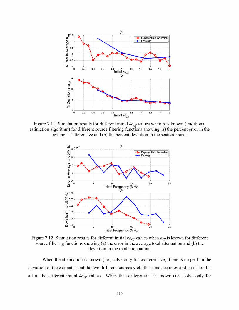
Figure 7.11: Simulation results for different initial kaeff values when α is known (traditional
estimation algorithm) for different source filtering functions showing (a) the percent error in the average scatterer size and (b) the percent deviation in the scatterer size.
Figure 7.12: Simulation results for different initial kaeff values when aeff is known for different
source filtering functions showing (a) the error in the average total attenuation and (b) the deviation in the total attenuation.
When the attenuation is known (i.e., solve only for scatterer size), there is no peak in the
deviation of the estimates and the two different sources yield the same accuracy and precision for
all of the different initial kaeff values. When the scatterer size is known (i.e., solve only for
119
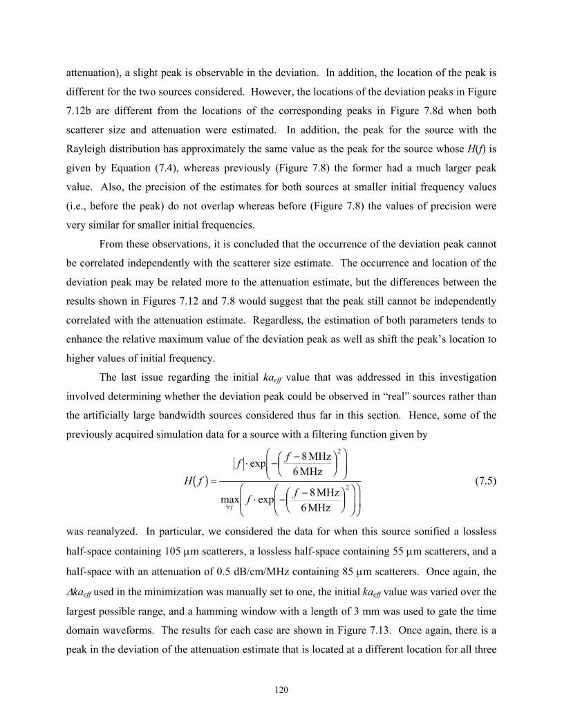
attenuation), a slight peak is observable in the deviation. In addition, the location of the peak is
different for the two sources considered. However, the locations of the deviation peaks in Figure
7.12b are different from the locations of the corresponding peaks in Figure 7.8d when both
scatterer size and attenuation were estimated. In addition, the peak for the source with the
Rayleigh distribution has approximately the same value as the peak for the source whose H(f) is
given by Equation (7.4), whereas previously (Figure 7.8) the former had a much larger peak
value. Also, the precision of the estimates for both sources at smaller initial frequency values
(i.e., before the peak) do not overlap whereas before (Figure 7.8) the values of precision were
very similar for smaller initial frequencies.
From these observations, it is concluded that the occurrence of the deviation peak cannot
be correlated independently with the scatterer size estimate. The occurrence and location of the
deviation peak may be related more to the attenuation estimate, but the differences between the
results shown in Figures 7.12 and 7.8 would suggest that the peak still cannot be independently
correlated with the attenuation estimate. Regardless, the estimation of both parameters tends to
enhance the relative maximum value of the deviation peak as well as shift the peak’s location to
higher values of initial frequency.
The last issue regarding the initial kaeff value that was addressed in this investigation
involved determining whether the deviation peak could be observed in “real” sources rather than
the artificially large bandwidth sources considered thus far in this section. Hence, some of the
previously acquired simulation data for a source with a filtering function given by
H ff f
f ff
b g =⋅ −
−FHG
IKJ
FHG
IKJ
⋅ −−FHG
IKJ
FHG
IKJ
FHG
IKJ∀
exp MHzMHz
max exp MHzMHz
86
86
2
2 (7.5)
was reanalyzed. In particular, we considered the data for when this source sonified a lossless
half-space containing 105 µm scatterers, a lossless half-space containing 55 µm scatterers, and a
half-space with an attenuation of 0.5 dB/cm/MHz containing 85 µm scatterers. Once again, the
∆kaeff used in the minimization was manually set to one, the initial kaeff value was varied over the
largest possible range, and a hamming window with a length of 3 mm was used to gate the time
domain waveforms. The results for each case are shown in Figure 7.13. Once again, there is a
peak in the deviation of the attenuation estimate that is located at a different location for all three
120
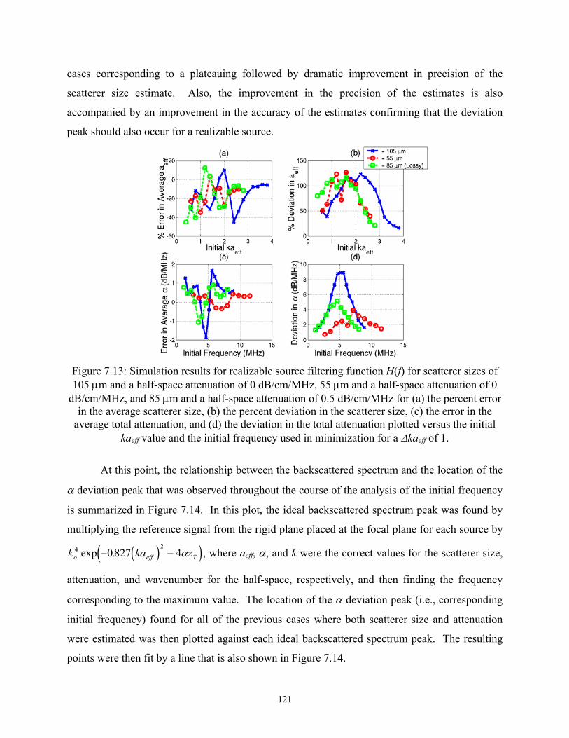
cases corresponding to a plateauing followed by dramatic improvement in precision of the
scatterer size estimate. Also, the improvement in the precision of the estimates is also
accompanied by an improvement in the accuracy of the estimates confirming that the deviation
peak should also occur for a realizable source.
Figure 7.13: Simulation results for realizable source filtering function H(f) for scatterer sizes of 105 µm and a half-space attenuation of 0 dB/cm/MHz, 55 µm and a half-space attenuation of 0
dB/cm/MHz, and 85 µm and a half-space attenuation of 0.5 dB/cm/MHz for (a) the percent error in the average scatterer size, (b) the percent deviation in the scatterer size, (c) the error in the
average total attenuation, and (d) the deviation in the total attenuation plotted versus the initial kaeff value and the initial frequency used in minimization for a ∆kaeff of 1.
At this point, the relationship between the backscattered spectrum and the location of the
α deviation peak that was observed throughout the course of the analysis of the initial frequency
is summarized in Figure 7.14. In this plot, the ideal backscattered spectrum peak was found by
multiplying the reference signal from the rigid plane placed at the focal plane for each source by
, where ak kao eff4 2
0 827 4exp .− −d ie αzT j eff, α, and k were the correct values for the scatterer size,
attenuation, and wavenumber for the half-space, respectively, and then finding the frequency
corresponding to the maximum value. The location of the α deviation peak (i.e., corresponding
initial frequency) found for all of the previous cases where both scatterer size and attenuation
were estimated was then plotted against each ideal backscattered spectrum peak. The resulting
points were then fit by a line that is also shown in Figure 7.14.
121
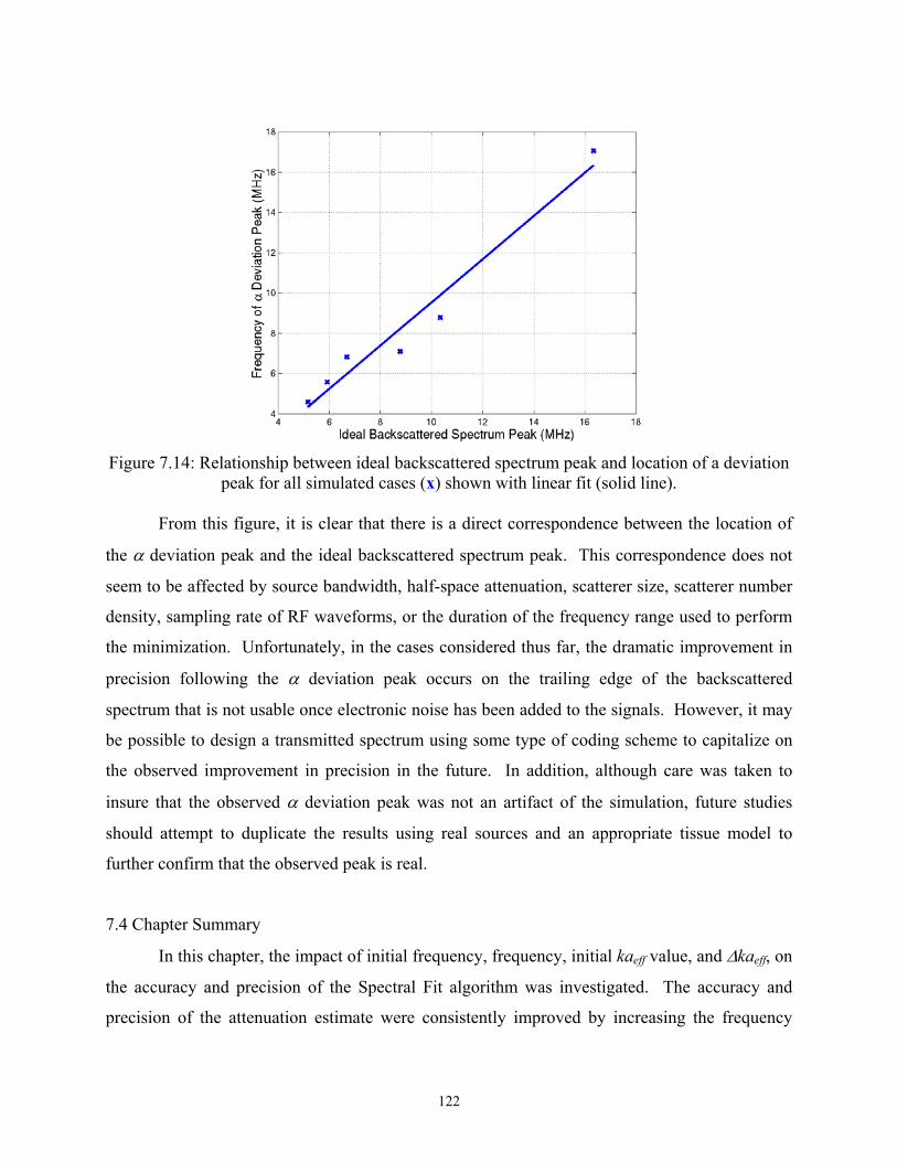
Figure 7.14: Relationship between ideal backscattered spectrum peak and location of a deviation
peak for all simulated cases (x) shown with linear fit (solid line).
From this figure, it is clear that there is a direct correspondence between the location of
the α deviation peak and the ideal backscattered spectrum peak. This correspondence does not
seem to be affected by source bandwidth, half-space attenuation, scatterer size, scatterer number
density, sampling rate of RF waveforms, or the duration of the frequency range used to perform
the minimization. Unfortunately, in the cases considered thus far, the dramatic improvement in
precision following the α deviation peak occurs on the trailing edge of the backscattered
spectrum that is not usable once electronic noise has been added to the signals. However, it may
be possible to design a transmitted spectrum using some type of coding scheme to capitalize on
the observed improvement in precision in the future. In addition, although care was taken to
insure that the observed α deviation peak was not an artifact of the simulation, future studies
should attempt to duplicate the results using real sources and an appropriate tissue model to
further confirm that the observed peak is real.
7.4 Chapter Summary
In this chapter, the impact of initial frequency, frequency, initial kaeff value, and ∆kaeff, on
the accuracy and precision of the Spectral Fit algorithm was investigated. The accuracy and
precision of the attenuation estimate were consistently improved by increasing the frequency
122
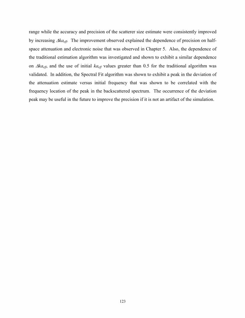
123
range while the accuracy and precision of the scatterer size estimate were consistently improved
by increasing ∆kaeff. The improvement observed explained the dependence of precision on half-
space attenuation and electronic noise that was observed in Chapter 5. Also, the dependence of
the traditional estimation algorithm was investigated and shown to exhibit a similar dependence
on ∆kaeff, and the use of initial kaeff values greater than 0.5 for the traditional algorithm was
validated. In addition, the Spectral Fit algorithm was shown to exhibit a peak in the deviation of
the attenuation estimate versus initial frequency that was shown to be correlated with the
frequency location of the peak in the backscattered spectrum. The occurrence of the deviation
peak may be useful in the future to improve the precision if it is not an artifact of the simulation.
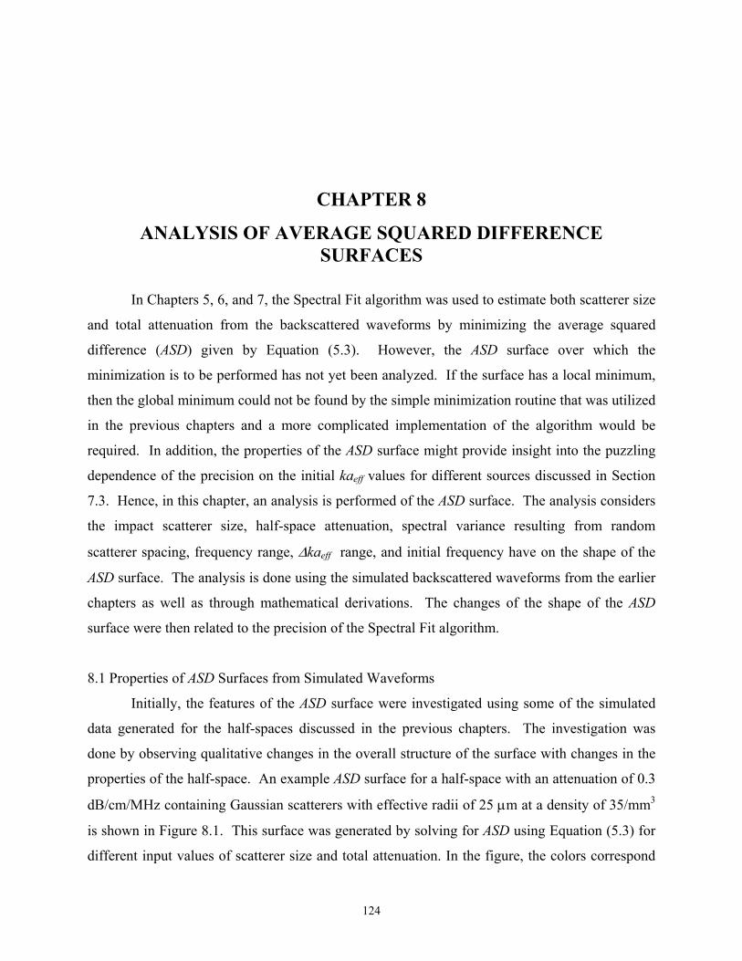
CHAPTER 8
ANALYSIS OF AVERAGE SQUARED DIFFERENCE SURFACES
In Chapters 5, 6, and 7, the Spectral Fit algorithm was used to estimate both scatterer size
and total attenuation from the backscattered waveforms by minimizing the average squared
difference (ASD) given by Equation (5.3). However, the ASD surface over which the
minimization is to be performed has not yet been analyzed. If the surface has a local minimum,
then the global minimum could not be found by the simple minimization routine that was utilized
in the previous chapters and a more complicated implementation of the algorithm would be
required. In addition, the properties of the ASD surface might provide insight into the puzzling
dependence of the precision on the initial kaeff values for different sources discussed in Section
7.3. Hence, in this chapter, an analysis is performed of the ASD surface. The analysis considers
the impact scatterer size, half-space attenuation, spectral variance resulting from random
scatterer spacing, frequency range, ∆kaeff range, and initial frequency have on the shape of the
ASD surface. The analysis is done using the simulated backscattered waveforms from the earlier
chapters as well as through mathematical derivations. The changes of the shape of the ASD
surface were then related to the precision of the Spectral Fit algorithm.
8.1 Properties of ASD Surfaces from Simulated Waveforms
Initially, the features of the ASD surface were investigated using some of the simulated
data generated for the half-spaces discussed in the previous chapters. The investigation was
done by observing qualitative changes in the overall structure of the surface with changes in the
properties of the half-space. An example ASD surface for a half-space with an attenuation of 0.3
dB/cm/MHz containing Gaussian scatterers with effective radii of 25 µm at a density of 35/mm3
is shown in Figure 8.1. This surface was generated by solving for ASD using Equation (5.3) for
different input values of scatterer size and total attenuation. In the figure, the colors correspond
124
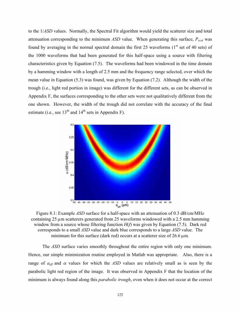
to the 1/ASD values. Normally, the Spectral Fit algorithm would yield the scatterer size and total
attenuation corresponding to the minimum ASD value. When generating this surface, Pscat was
found by averaging in the normal spectral domain the first 25 waveforms (1st set of 40 sets) of
the 1000 waveforms that had been generated for this half-space using a source with filtering
characteristics given by Equation (7.5). The waveforms had been windowed in the time domain
by a hamming window with a length of 2.5 mm and the frequency range selected, over which the
mean value in Equation (5.3) was found, was given by Equation (7.2). Although the width of the
trough (i.e., light red portion in image) was different for the different sets, as can be observed in
Appendix F, the surfaces corresponding to the other sets were not qualitatively different from the
one shown. However, the width of the trough did not correlate with the accuracy of the final
estimate (i.e., see 13th and 14th sets in Appendix F).
Figure 8.1: Example ASD surface for a half-space with an attenuation of 0.3 dB/cm/MHz
containing 25 µm scatterers generated from 25 waveforms windowed with a 2.5 mm hamming window from a source whose filtering function H(f) was given by Equation (7.5). Dark red
corresponds to a small ASD value and dark blue corresponds to a large ASD value. The minimum for this surface (dark red) occurs at a scatterer size of 26.6 µm.
The ASD surface varies smoothly throughout the entire region with only one minimum.
Hence, our simple minimization routine employed in Matlab was appropriate. Also, there is a
range of aeff and α values for which the ASD values are relatively small as is seen by the
parabolic light red region of the image. It was observed in Appendix F that the location of the
minimum is always found along this parabolic trough, even when it does not occur at the correct
125

value for scatterer size and total attenuation. The parabolic trough is symmetric about aeff = 0
µm because aeff is squared in the evaluation of the Gaussian form factor. Of course, a negative
value for scatterer size is not physical and hence would only be a mathematical peculiarity.
After establishing the basic shape of the ASD surface, the influence of the different half-
space parameters on this basic shape was investigated. Hence, an ASD surface, shown in Figure
8.2, was generated corresponding to the first 25 waveforms (1st set of 40 sets) for a half-space
with a half-space attenuation of 0.5 dB/cm/MHz that still contained Gaussian scatterers with
effective radii of 25 µm at a density of 35/mm3. The frequency range was once again selected by
Equation (7.2) and a hamming window with a length of 2.5 mm was still used to gate the time
domain signals. Now the parabolic trough intersects the aeff = 0 µm axis at ~0.55 dB/cm/MHz.
However, the same change in scatterer size results in the same change in attenuation along the
parabolic trough. Hence, the attenuation appears to shift the surface to higher values of
attenuation without affecting the overall shape of the surface.
Figure 8.2: Example ASD surface for a half-space with an attenuation of 0.5 dB/cm/MHz
containing 25 µm scatterers generated from 25 waveforms windowed with a 2.5 mm hamming window from a source whose filtering function H(f) was given by Equation (7.5). Dark red
corresponds to a small ASD value and dark blue corresponds to a large ASD value. The minimum for this surface (dark red) occurs at a scatterer size of 18.0 µm.
After assessing the impact of attenuation on the ASD surface, the effect of different
scatterer sizes was evaluated. Hence, ASD surfaces, shown in Figures 8.3 and 8.4, were
126

generated corresponding to two half-spaces containing scatterers with aeff of 5 µm and 45 µm,
respectively. The attenuation of the half-spaces was maintained at 0.3 dB/cm/MHz while the
source and windowing parameters were the same as the previous two surface plots. Once again,
the different scatterer sizes appear to primarily shift the ASD surfaces along the α axis with the
smaller scatterer sizes shifting the surface to smaller α values and the larger scatterer size
shifting the surface to large α values. However, the area colored light red in the figures relative
to the true scatterer size appears to be much smaller as the scatterer size is increased. Hence, the
minimum is more pronounced for the larger sized scatterers.
Once the impact of attenuation and scatterer size on the ASD surface was determined, the
influence of window length was investigated because the earlier results indicated that the
precision of the estimates should be improved by increasing the length of the window used to
gate the time domain signals. Figure 8.5 shows the ASD surface for the same waveforms used to
generate the ASD surface in Figure 8.2, only with a hamming window of length of 8 mm instead
of 2.5 mm. The ASD surface in Figure 8.5 is indistinguishable from the ASD surface in Figure
8.2. Hence, although the larger window lengths improve the precision of the Spectral Fit
algorithm, the improvement does not appear to result from any changes to the overall structure of
the ASD surface. However, it may be that the changes are not visible in this simple qualitative
comparison of the surfaces.
After exploring the impact of window length, the effect of different frequency ranges on
the ASD surface, while maintaining the same ∆kaeff range, was investigated. Figure 8.6 shows
the ASD surface corresponding to the first 25 waveforms (1st set of 40 sets) of the 1000
waveforms that had been generated for a half-space with an attenuation of 0 dB/cm/MHz
containing Gaussian scatterers with effective radii of 25 µm. The source used to generate the
waveforms had filtering characteristics given by Equation (7.4), and the waveforms had been
windowed in the time domain by a hamming window with a length of 3 mm. Frequencies
corresponding to kaeff values of 0.5 to 1.5 were used to find the ASD. Likewise, Figure 8.7
shows the ASD surface corresponding to the first 25 waveforms (1st set of 40 sets) of the 1000
waveforms that had been generated for a half-space with an attenuation of 0 dB/cm/MHz
containing scatterers with effective radii of 50 µm using the same source and window length.
The frequency range for Figure 8.7 was given by the frequencies corresponding to kaeff values of
1 to 2 (same initial frequency and ∆kaeff range but different frequency range).
127

Figure 8.3: Example ASD surface for a half-space with an attenuation of 0.3 dB/cm/MHz
containing 5 µm scatterers generated from 25 waveforms windowed with a 2.5 mm hamming window from a source whose filtering function H(f) was given by Equation (7.5). Dark red
corresponds to a small ASD value and dark blue corresponds to a large ASD value. The minimum for this surface (dark red) occurs at a scatterer size of 13.2 µm.
Figure 8.4: Example ASD surface for a half-space with an attenuation of 0.3 dB/cm/MHz
containing 45 µm scatterers generated from 25 waveforms windowed with a 2.5 mm hamming window from a source whose filtering function H(f) was given by Equation (7.5). Dark red
corresponds to a small ASD value and dark blue corresponds to a large ASD value. The minimum for this surface (dark red) occurs at a scatterer size of 43.0 µm.
128
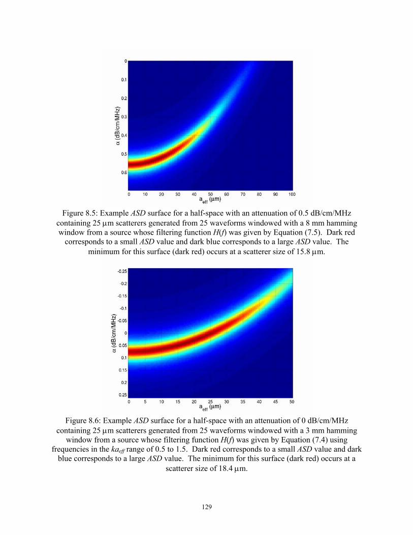
Figure 8.5: Example ASD surface for a half-space with an attenuation of 0.5 dB/cm/MHz
containing 25 µm scatterers generated from 25 waveforms windowed with a 8 mm hamming window from a source whose filtering function H(f) was given by Equation (7.5). Dark red
corresponds to a small ASD value and dark blue corresponds to a large ASD value. The minimum for this surface (dark red) occurs at a scatterer size of 15.8 µm.
Figure 8.6: Example ASD surface for a half-space with an attenuation of 0 dB/cm/MHz
containing 25 µm scatterers generated from 25 waveforms windowed with a 3 mm hamming window from a source whose filtering function H(f) was given by Equation (7.4) using
frequencies in the kaeff range of 0.5 to 1.5. Dark red corresponds to a small ASD value and dark blue corresponds to a large ASD value. The minimum for this surface (dark red) occurs at a
scatterer size of 18.4 µm.
129

Figure 8.7: Example ASD surface for a half-space with an attenuation of 0 dB/cm/MHz
containing 50 µm scatterers generated from 25 waveforms windowed with a 3 mm hamming window from a source whose filtering function H(f) was given by Equation (7.4) using
frequencies in the kaeff range of 1 to 2. Dark red corresponds to a small ASD value and dark blue corresponds to a large ASD value. The minimum for this surface (dark red) occurs at a scatterer
size of .0196 nm.
By comparing Figures 8.6 and 8.7, one can observe that the ASD surface has once again
been shifted to larger α values for the larger scatterer size. Furthermore, the parabola describing
the parabolic trough has been broadened when a smaller frequency range was used (Figure 8.7).
Hence, a change in aeff produces a smaller change in α along the trough in Figure 8.7 as
compared to Figure 8.6. Also, the minimum is more pronounced for the smaller sized scatterers
when the larger frequency range was selected. When compared to the results in Figure 8.4, this
suggests that the more pronounced minimum observed earlier for the larger scatterer sizes was
probably due to the increased ∆kaeff range just as the more pronounced minimum in this case is
probably due to the increased frequency range.
Another effect observed in Chapter 7 was the dependence of the precision on the initial
frequency used in the minimization routine (i.e., Section 7.3). This dependence was also shown
to be related to the peak frequency of the ideal backscattered spectrum. Hence, the next goal was
to determine if the dependence on the initial frequency and the corresponding relationship to the
peak of the backscattered spectrum could be observed by analyzing the appropriate ASD
surfaces.
130
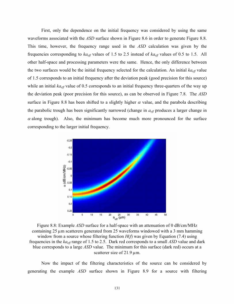
First, only the dependence on the initial frequency was considered by using the same
waveforms associated with the ASD surface shown in Figure 8.6 in order to generate Figure 8.8.
This time, however, the frequency range used in the ASD calculation was given by the
frequencies corresponding to kaeff values of 1.5 to 2.5 instead of kaeff values of 0.5 to 1.5. All
other half-space and processing parameters were the same. Hence, the only difference between
the two surfaces would be the initial frequency selected for the calculation. An initial kaeff value
of 1.5 corresponds to an initial frequency after the deviation peak (good precision for this source)
while an initial kaeff value of 0.5 corresponds to an initial frequency three-quarters of the way up
the deviation peak (poor precision for this source), as can be observed in Figure 7.8. The ASD
surface in Figure 8.8 has been shifted to a slightly higher α value, and the parabola describing
the parabolic trough has been significantly narrowed (change in aeff produces a larger change in
α along trough). Also, the minimum has become much more pronounced for the surface
corresponding to the larger initial frequency.
Figure 8.8: Example ASD surface for a half-space with an attenuation of 0 dB/cm/MHz
containing 25 µm scatterers generated from 25 waveforms windowed with a 3 mm hamming window from a source whose filtering function H(f) was given by Equation (7.4) using
frequencies in the kaeff range of 1.5 to 2.5. Dark red corresponds to a small ASD value and dark blue corresponds to a large ASD value. The minimum for this surface (dark red) occurs at a
scatterer size of 21.9 µm.
Now the impact of the filtering characteristics of the source can be considered by
generating the example ASD surface shown in Figure 8.9 for a source with filtering
131

characteristics given by Equation (7.1) with a σR of 18 MHz and a fo of 8 MHz. All of the half-
space and processing parameters will be the same as the surface shown in Figure 8.8, including
the selection of frequencies corresponding to kaeff values of 1.5 to 2.5. An initial kaeff value of
1.5 corresponds to an initial frequency close to the top of the deviation peak (poor precision) for
this source as can be observed in Figure 7.8. The parabola describing the parabolic trough has
basically the same width and position in Figure 8.9 as in Figure 8.8. Also, the minimum is much
less pronounced for the ASD surface shown in Figure 8.9 as compared to Figure 8.8 and is about
as pronounced as the minimum in Figure 8.6. However, the reason for the peak being more
pronounced in Figure 8.8 cannot be deduced based on a qualitative comparison of the different
ASD surfaces.
Figure 8.9: Example ASD surface for a half-space with an attenuation of 0 dB/cm/MHz
containing 25 µm scatterers generated from 25 waveforms windowed with a 3 mm hamming window from a source whose filtering function H(f) was given by Equation (7.1) with a σR of 18 MHz and a fo of 8 MHz using frequencies in the kaeff range of 1.5 to 2.5. Dark red corresponds to a small ASD value and dark blue corresponds to a large ASD value. The minimum for this
surface (dark red) occurs at a scatterer size of 25.6 µm.
8.2 Mathematical Derivation and Analysis of Ideal ASD Surfaces
In the previous section, the impacts of attenuation, scatterer size, window length,
frequency range, initial frequency, and source filtering function were investigated by looking at
example ASD surfaces for some of the previously simulated waveforms. To better understand
these example surfaces, a mathematical description of the surface is derived in this section. The
132

derivation can then be used to provide additional insight into the minimization of the ASD
surface.
8.2.1 Derivation of ASD surface
To begin the derivation of the surface, assume the expression for X(f,aeff,αo) from
Equation (5.4) can be written as
X f aP f
P fP f e e
P f e e
C P f f e eP f
P f e e
P f e
eff oscat
f scat
refka fz
f refka fz
ref ska fz
f scat
refka fz
f ref
eff o T
eff o T
real real T eff o T
, , lnmax
lnmax
lnmax
lnmax
.
.
. .
α
ξ
α
α
α α
d i b gb gc h
b gb g
b g b gb gc h
b gb g
d i
d i
b g d i
=FHGG
IKJJ − F
HIK
F
HGGG
I
KJJJ
=FHGG
IKJJ −
− −
− −
− − − −
0 827 4
0 827 4
10 827 4 0 827 4
2
2
2 2
− −FH
IK
F
HGGG
I
KJJJ
= − FHGIKJ − − − +
0 827 4
22 2 2
2
2
0827 2 4
.
ln . ,
ka fz
s real eff T real o
eff o Te
fc
f a a z f C
d i
b gc h d i b g
α
ξ π α α
(8.1)
where C1 and C2 are constants independent of frequency related to the acoustic concentration and
transmission coefficient for the intervening tissue layers, areal and αreal are the real values of
scatterer size and attenuation respectively, and ξs(f) are the spectral fluctuations related to the
random scatterer spacing. Hence, X becomes
X a fc
a a f
z f C
eff o f s real eff f
T real o f
, mean ln . mean
mean
α ξ π
α α
d i b gc h d ib g
= − FHGIKJ −
− − +
0 827 2
4
22 2
2
2
(8.2)
and
X X f fc
a a f f
z f f
s f s real eff f
T real o f
− = −FH IK −FHGIKJ − −FH IK
− − −FH IK
ln mean ln . mean
mean
ξ ξ π
α α
b gc h b gc h d i
b g
0827 2
4
22 2 2 2
(8.3)
yielding
133
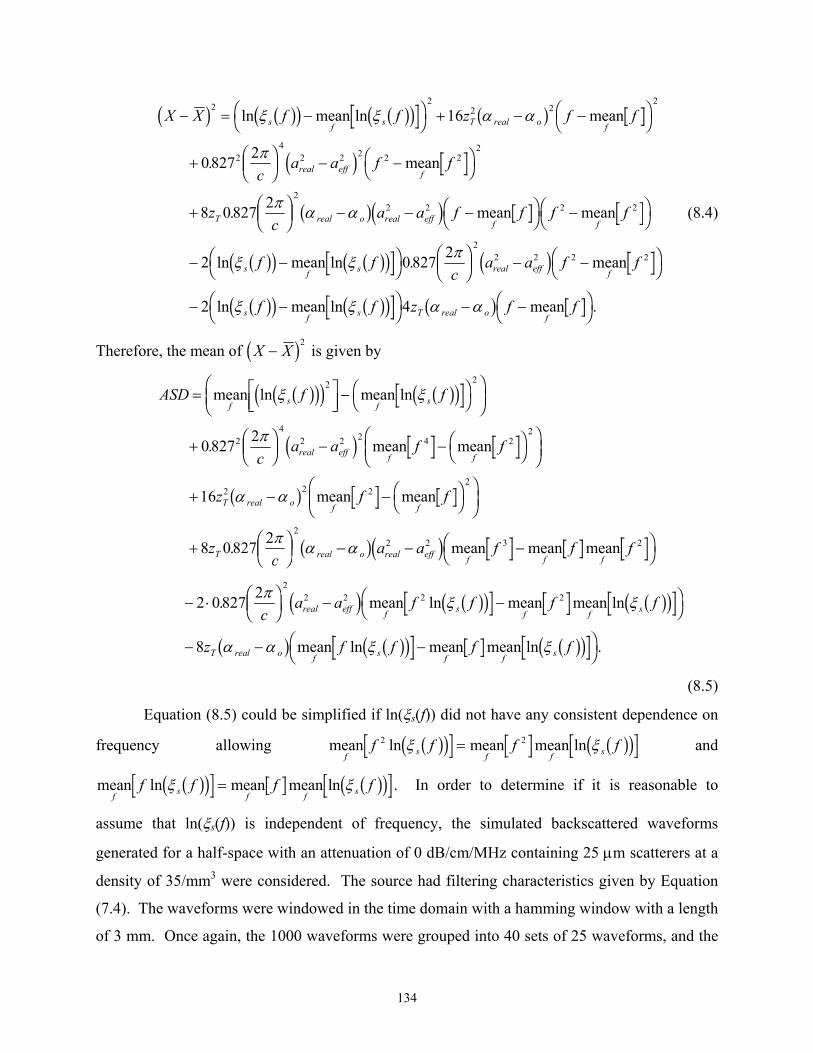
X X f f z f f
ca a f f
zc
a a f f f f
f fc
s f s T real o f
real eff f
T real o real eff f f
s f s
− = −FH IK + − −FH IK+ F
HGIKJ − −FH IK
+ FHGIKJ − − −FH IK −FH IK
− −FH IKFH
c h b gc h b gc h b g
d i
b gd i
b gc h b gc h
22
2 22
24
2 2 2 2 22
22 2 2 2
16
0827 2
8 0827 2
2 0827 2
ln mean ln mean
. mean
. mean
ln mean ln .
ξ ξ α α
π
π α α
ξ ξ π
mean
G IKJ − −FH IK− −FH IK − −FH IK
22 2 2 2
2 4
a a f f
f f z f f
real eff f
s f s T real o f
d i
b gc h b gc h b g
mean
ln mean ln mean .ξ ξ α α
(8.4)
Therefore, the mean of X X−2c is given by h
ASD f f
ca a f f
z f f
zc
a a f f f
f s f s
real eff f f
T real o f f
T real o real eff f f f
= LNM OQP −FH IK
FHG
IKJ
+ FHGIKJ − − FH IK
FHG
IKJ
+ − − FH IKFHG
IKJ
+ FHGIKJ − − −FH IK
mean ln mean ln
. mean mean
mean mean
. mean mean mean
ξ ξ
π
α α
π α α
b gc hd i b gc h
d i
b g
b gd i
2 2
24
2 2 2 4 22
2 2 22
22 2 3 2
0827 2
16
8 0827 2
− ⋅ F
HGIKJ − −FH IK
− − −FH IK
2 0827 2
8
22 2 2 2. mean ln mean mean ln
mean ln mean mean ln .
π ξ ξ
α α ξ ξ
ca a f f f f
z f f f f
real eff f s f f s
T real o f s f f s
d i b gc h b gc h
b g b gc h b gc h
(8.5)
Equation (8.5) could be simplified if ln(ξs(f)) did not have any consistent dependence on
frequency allowing m and ean ln mean mean lnf s f f sf f f2 2ξ b gc h b gc= fξ h
mean ln mean mean lnf s f f sf f f fξ b gc h b gc h= ξ . In order to determine if it is reasonable to
assume that ln(ξs(f)) is independent of frequency, the simulated backscattered waveforms
generated for a half-space with an attenuation of 0 dB/cm/MHz containing 25 µm scatterers at a
density of 35/mm3 were considered. The source had filtering characteristics given by Equation
(7.4). The waveforms were windowed in the time domain with a hamming window with a length
of 3 mm. Once again, the 1000 waveforms were grouped into 40 sets of 25 waveforms, and the
134

25 waveforms in each set were averaged in the normal spectral domain to obtain 40 estimates for
the Pscat versus frequency curves for frequencies corresponding to kaeff values between 0.1 and 3.
Each Pscat curve was then divided by ma and evaluated as a
natural log in order to obtain 40 examples of ln(C
x .
f scat refka fzP f P f e ereal real Tb gc h b g b g− −0 827 42 α
1ξs(f)). These 40 examples were then averaged
together and the resulting estimate of ln mean lnξ ξs f sf fb gc h b gc h−FH IK versus frequency was
plotted in Figure 8.10. Clearly, on average ln(ξs(f)) does not exhibit any consistent frequency
dependence. As a result, Equation (8.5) can be simplified as
f
f f
z f f
a a f
f s
f f
f f
eal o real eff f f
FH IKIKJ
− − FH IKFHG
IKJ
− FH IKIKJ
− − FH
mean ln
mean mean
mean
mean m
ξ ξ
α α
b gc h
d i
gd i
2
2 4 22
22
2 2 3
(8.6)
ASD f
ca a
zc
f f
f s
real eff
T real o
T r f
= LNM OQP −FHG
+ FHGIKJ
+ −FHG
+ FHGIKJ − IK
mean ln
.
mean
. ean mean .
π
α α
π
b gc hd i
b g
b
2
24
2 2
2 2
22
0827 2
16
8 0827 2
Figure 8.10: ln mean lnξ ξs f sfb gc h b gc h− fFH IK for waveforms from a half space with an attenuation
of 0 dB/cm/MHz containing 25 µm scatterers at a density of 35/mm3. The source had filtering characteristics given by Equation (7.4).
Frequency (MHz)
ln(ξ
s(f))
-mea
n(ln
(ξs(f
)))
135
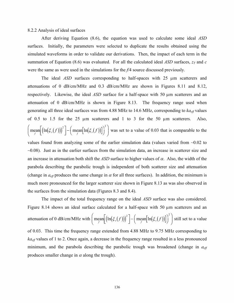
8.2.2 Analysis of ideal surfaces
After deriving Equation (8.6), the equation was used to calculate some ideal ASD
surfaces. Initially, the parameters were selected to duplicate the results obtained using the
simulated waveforms in order to validate our derivations. Then, the impact of each term in the
summation of Equation (8.6) was evaluated. For all the calculated ideal ASD surfaces, zT and c
were the same as were used in the simulations for the f/4 source discussed previously.
The ideal ASD surfaces corresponding to half-spaces with 25 µm scatterers and
attenuations of 0 dB/cm/MHz and 0.3 dB/cm/MHz are shown in Figures 8.11 and 8.12,
respectively. Likewise, the ideal ASD surface for a half-space with 50 µm scatterers and an
attenuation of 0 dB/cm/MHz is shown in Figure 8.13. The frequency range used when
generating all three ideal surfaces was from 4.88 MHz to 14.6 MHz, corresponding to kaeff values
of 0.5 to 1.5 for the 25 µm scatterers and 1 to 3 for the 50 µm scatterers. Also,
mean ln mean lnf s f sfξ ξb gc hd i b gc h2 2LNM OQP − fFH IKFHG
IKJ was set to a value of 0.03 that is comparable to the
values found from analyzing some of the earlier simulation data (values varied from ~0.02 to
~0.08). Just as in the earlier surfaces from the simulation data, an increase in scatterer size and
an increase in attenuation both shift the ASD surface to higher values of α. Also, the width of the
parabola describing the parabolic trough is independent of both scatterer size and attenuation
(change in aeff produces the same change in α for all three surfaces). In addition, the minimum is
much more pronounced for the larger scatterer size shown in Figure 8.13 as was also observed in
the surfaces from the simulation data (Figures 8.3 and 8.4).
The impact of the total frequency range on the ideal ASD surface was also considered.
Figure 8.14 shows an ideal surface calculated for a half-space with 50 µm scatterers and an
attenuation of 0 dB/cm/MHz with mean ln mean lnf s f sfξ ξb gc hd i b gc h2 2
fLNM OQP −FH IK
FHG
IKJ still set to a value
of 0.03. This time the frequency range extended from 4.88 MHz to 9.75 MHz corresponding to
kaeff values of 1 to 2. Once again, a decrease in the frequency range resulted in a less pronounced
minimum, and the parabola describing the parabolic trough was broadened (change in aeff
produces smaller change in α along the trough).
136

Figure 8.11: Ideal ASD surface for a half-space with an attenuation of 0 dB/cm/MHz containing
25 µm scatterers using frequencies in the kaeff range of 0.5 to 1.5 for a
mean ln mean lnf s f sfξ ξb gc hd i b gc h2 2LNM OQP − fFH IKFHG
IKJ value of 0.03. Dark red corresponds to a small ASD
value and dark blue corresponds to a large ASD value.
Figure 8.12: Ideal ASD surface for a half-space with an attenuation of 0.3 dB/cm/MHz
containing 25 µm scatterers using frequencies in the kaeff range of 0.5 to 1.5 for a
mean ln mean lnf s f sfξ ξb gc hd i b gc h2 2LNM OQP − fFH IKFHG
IKJ value of 0.03. Dark red corresponds to a small ASD
value and dark blue corresponds to a large ASD value.
137
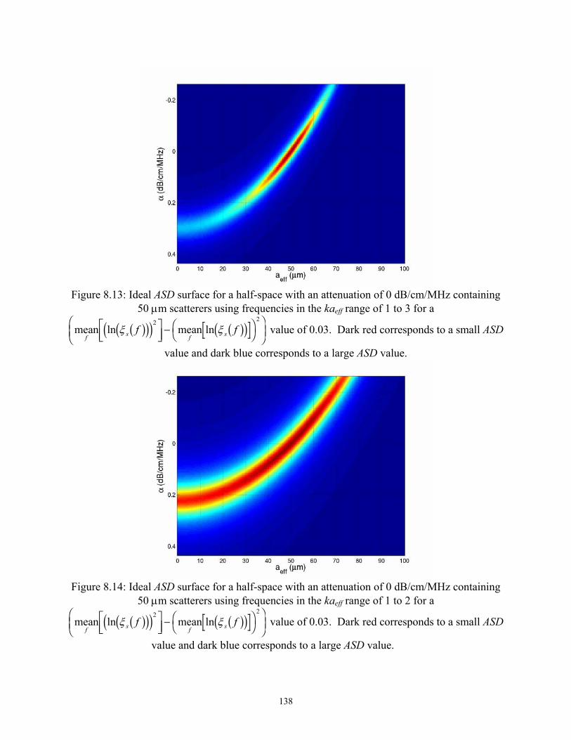
Figure 8.13: Ideal ASD surface for a half-space with an attenuation of 0 dB/cm/MHz containing
50 µm scatterers using frequencies in the kaeff range of 1 to 3 for a
mean ln mean lnf s f sfξ ξb gc hd i b gc h2 2LNM OQP − fFH IKFHG
IKJ value of 0.03. Dark red corresponds to a small ASD
value and dark blue corresponds to a large ASD value.
Figure 8.14: Ideal ASD surface for a half-space with an attenuation of 0 dB/cm/MHz containing
50 µm scatterers using frequencies in the kaeff range of 1 to 2 for a
mean ln mean lnf s f sfξ ξb gc hd i b gc h2 2LNM OQP − fFH IKFHG
IKJ value of 0.03. Dark red corresponds to a small ASD
value and dark blue corresponds to a large ASD value.
138
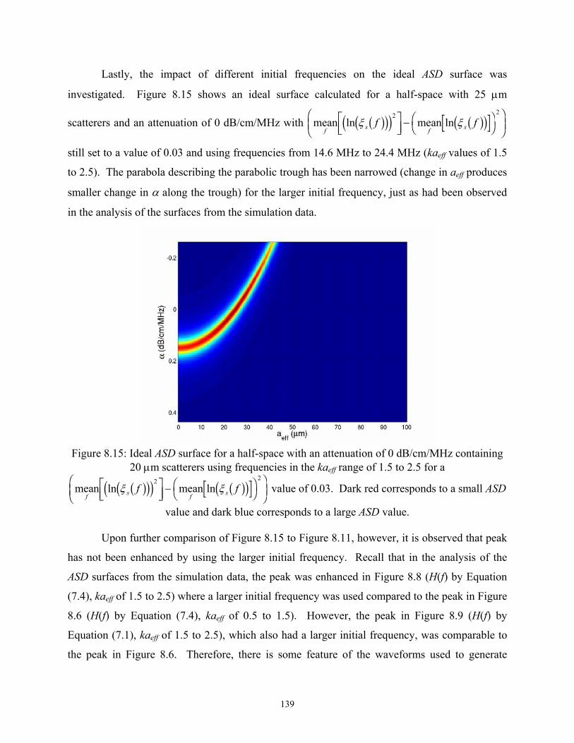
Lastly, the impact of different initial frequencies on the ideal ASD surface was
investigated. Figure 8.15 shows an ideal surface calculated for a half-space with 25 µm
scatterers and an attenuation of 0 dB/cm/MHz with mean ln mean lnf s f sf fξ ξb gc hd i b gc h2 2LNM OQP −
FH IKFHG
IKJ
still set to a value of 0.03 and using frequencies from 14.6 MHz to 24.4 MHz (kaeff values of 1.5
to 2.5). The parabola describing the parabolic trough has been narrowed (change in aeff produces
smaller change in α along the trough) for the larger initial frequency, just as had been observed
in the analysis of the surfaces from the simulation data.
Figure 8.15: Ideal ASD surface for a half-space with an attenuation of 0 dB/cm/MHz containing
20 µm scatterers using frequencies in the kaeff range of 1.5 to 2.5 for a
mean ln mean lnf s f sfξ ξb gc hd i b gc h2 2LNM OQP − fFH IKFHG
IKJ value of 0.03. Dark red corresponds to a small ASD
value and dark blue corresponds to a large ASD value.
Upon further comparison of Figure 8.15 to Figure 8.11, however, it is observed that peak
has not been enhanced by using the larger initial frequency. Recall that in the analysis of the
ASD surfaces from the simulation data, the peak was enhanced in Figure 8.8 (H(f) by Equation
(7.4), kaeff of 1.5 to 2.5) where a larger initial frequency was used compared to the peak in Figure
8.6 (H(f) by Equation (7.4), kaeff of 0.5 to 1.5). However, the peak in Figure 8.9 (H(f) by
Equation (7.1), kaeff of 1.5 to 2.5), which also had a larger initial frequency, was comparable to
the peak in Figure 8.6. Therefore, there is some feature of the waveforms used to generate
139
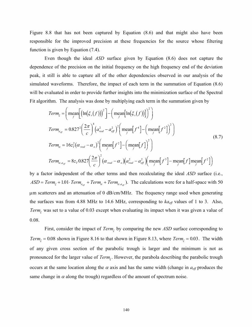
Figure 8.8 that has not been captured by Equation (8.6) and that might also have been
responsible for the improved precision at these frequencies for the source whose filtering
function is given by Equation (7.4).
Even though the ideal ASD surface given by Equation (8.6) does not capture the
dependence of the precision on the initial frequency on the high frequency end of the deviation
peak, it still is able to capture all of the other dependencies observed in our analysis of the
simulated waveforms. Therefore, the impact of each term in the summation of Equation (8.6)
will be evaluated in order to provide further insights into the minimization surface of the Spectral
Fit algorithm. The analysis was done by multiplying each term in the summation given by
Term f f
Termc
a a f f
Term z f f
Term zc
a a f f f
f s f s
a real eff f f
T real o f f
a T real o real eff f f f
eff
eff
ξ
α
α
ξ ξ
π
α α
π α α
= LNM OQP −FH IK
FHG
IKJ
= FHGIKJ − − FH IK
FHG
IKJ
= − − FH IKFHG
IKJ
= FHGIKJ − − −
mean ln mean ln
. mean mean
mean mean
. mean mean mean,
b gc hd i b gc h
d i
b g
b gd i
2 2
24
2 2 2 4 22
2 2 22
22 2 3
0827 2
16
8 0827 2 2FH IK
(8.7)
by a factor independent of the other terms and then recalculating the ideal ASD surface (i.e.,
ASD Term Term Term Termaeff eff= + ⋅ + a+ξ α101. ,
Termξ
α ). The calculations were for a half-space with 50
µm scatterers and an attenuation of 0 dB/cm/MHz. The frequency range used when generating
the surfaces was from 4.88 MHz to 14.6 MHz, corresponding to kaeff values of 1 to 3. Also,
was set to a value of 0.03 except when evaluating its impact when it was given a value of
0.08.
First, consider the impact of Termξ by comparing the new ASD surface corresponding to
shown in Figure 8.16 to that shown in Figure 8.13, where Term . The width
of any given cross section of the parabolic trough is larger and the minimum is not as
pronounced for the larger value of Termξ . However, the parabola describing the parabolic trough
occurs at the same location along the α axis and has the same width (change in a
Termξ = 0 08. ξ = 0 03.
eff produces the
same change in α along the trough) regardless of the amount of spectrum noise.
140

Figure 8.16: Ideal ASD surface to evaluate impact of Term using a half-space with an
attenuation of 0 dB/cm/MHz containing 50 µm scatterers using frequencies in the kaξ
eff range of 1 to 3 for Term . Dark red corresponds to a small ASD value and dark blue corresponds to a
large ASD value. ξ = 0 08.
In Section 8.1, some observations were made regarding the relative importance of the
minimum as half-space parameters, such as the scatterer size, and selected frequencies were
varied for the simulated waveforms. However, the amount of spectral variation (i.e., Termξ ) can
vary for different waveform sets and frequencies for the same half-space depending upon the
random arrangement of the scatterers. Since Termξ can influence the relative importance of the
minimum, the previous observations need to be validated by estimating Termξ for each of the
ASD plots from the simulated waveforms. The estimates for each of the surfaces were found by
dividing each Pscat curve by ma to obtain an estimate of
ln(C
x .
f scatka fzP f e ereal real Tb gc h b g− −0 827 42 α
refP fb g1ξ(f)) from which Term was then calculated. The Termξ values for all of the previous ASD
curves for the simulated waveforms are given in Table 8.1. The Termξ values for the simulated
cases are all approximately the same except for Figure 8.7 that is significantly less. When we
compared Figure 8.7 to 8.6 previously, the minimum of the ASD surface was less pronounced for
the larger sized scatterers using the smaller frequency range (Figure 8.7). However, the smaller
value of Figure 8.7 should have resulted in a more pronounced minimum in the absence of
ξ
Termξ
141
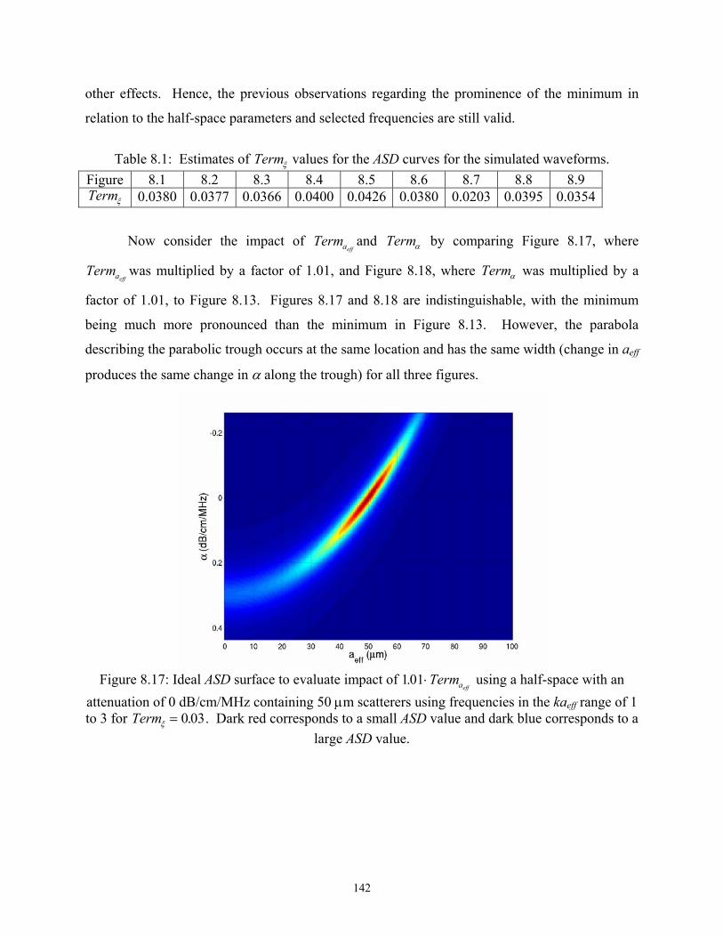
other effects. Hence, the previous observations regarding the prominence of the minimum in
relation to the half-space parameters and selected frequencies are still valid.
Table 8.1: Estimates of Term values for the ASD curves for the simulated waveforms. ξ
Figure 8.1 8.2 8.3 8.4 8.5 8.6 8.7 8.8 8.9 Termξ 0.0380 0.0377 0.0366 0.0400 0.0426 0.0380 0.0203 0.0395 0.0354
Now consider the impact of Te and by comparing Figure 8.17, where
was multiplied by a factor of 1.01, and Figure 8.18, where Term was multiplied by a
factor of 1.01, to Figure 8.13. Figures 8.17 and 8.18 are indistinguishable, with the minimum
being much more pronounced than the minimum in Figure 8.13. However, the parabola
describing the parabolic trough occurs at the same location and has the same width (change in a
rmaeffTermα
Termaeff α
eff
produces the same change in α along the trough) for all three figures.
Figure 8.17: Ideal ASD surface to evaluate impact of 101. ⋅Termaeff
using a half-space with an attenuation of 0 dB/cm/MHz containing 50 µm scatterers using frequencies in the kaeff range of 1 to 3 for Term . Dark red corresponds to a small ASD value and dark blue corresponds to a
large ASD value. ξ = 0 03.
142
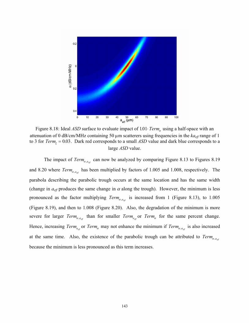
Figure 8.18: Ideal ASD surface to evaluate impact of 101. ⋅Termα using a half-space with an
attenuation of 0 dB/cm/MHz containing 50 µm scatterers using frequencies in the kaeff range of 1 to 3 for Term . Dark red corresponds to a small ASD value and dark blue corresponds to a
large ASD value. ξ = 0 03.
The impact of Term can now be analyzed by comparing Figure 8.13 to Figures 8.19
and 8.20 where Term has been multiplied by factors of 1.005 and 1.008, respectively. The
parabola describing the parabolic trough occurs at the same location and has the same width
(change in a
aeffα ,
aeffα ,
aeffα ,
rmaeff
eff produces the same change in α along the trough). However, the minimum is less
pronounced as the factor multiplying Term is increased from 1 (Figure 8.13), to 1.005
(Figure 8.19), and then to 1.008 (Figure 8.20). Also, the degradation of the minimum is more
severe for larger Term than for smaller Term or for the same percent change.
Hence, increasing Te or Term may not enhance the minimum if Term is also increased
at the same time. Also, the existence of the parabolic trough can be attributed to Term
because the minimum is less pronounced as this term increases.
aeffα ,
aeffTermα
α aeffα ,
aeffα ,
143
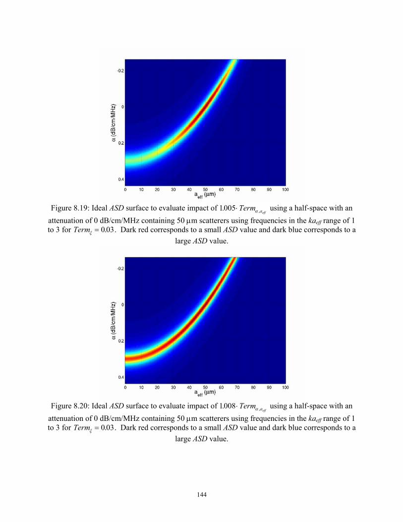
Figure 8.19: Ideal ASD surface to evaluate impact of 1005. ,⋅Term aeffα using a half-space with an
attenuation of 0 dB/cm/MHz containing 50 µm scatterers using frequencies in the kaeff range of 1 to 3 for Term . Dark red corresponds to a small ASD value and dark blue corresponds to a
large ASD value. ξ = 0 03.
Figure 8.20: Ideal ASD surface to evaluate impact of 1008. ,⋅Term aeffα using a half-space with an
attenuation of 0 dB/cm/MHz containing 50 µm scatterers using frequencies in the kaeff range of 1 to 3 for Term . Dark red corresponds to a small ASD value and dark blue corresponds to a
large ASD value. ξ = 0 03.
144
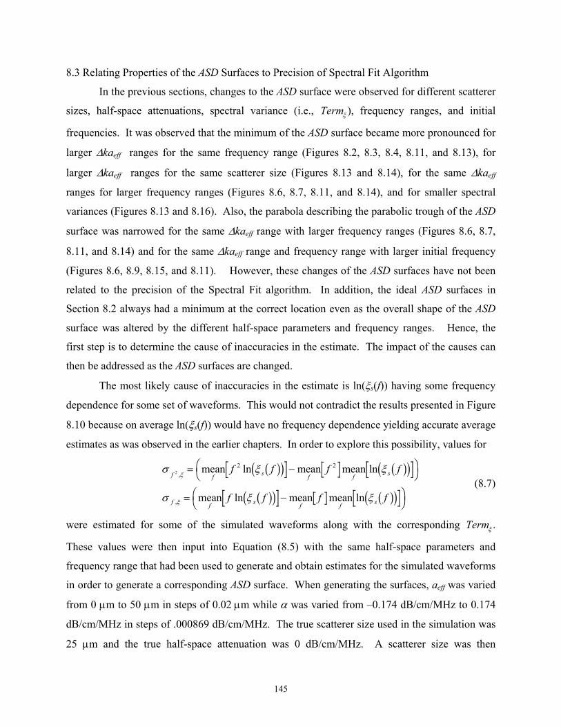
8.3 Relating Properties of the ASD Surfaces to Precision of Spectral Fit Algorithm
In the previous sections, changes to the ASD surface were observed for different scatterer
sizes, half-space attenuations, spectral variance (i.e., Termξ ), frequency ranges, and initial
frequencies. It was observed that the minimum of the ASD surface became more pronounced for
larger ∆kaeff ranges for the same frequency range (Figures 8.2, 8.3, 8.4, 8.11, and 8.13), for
larger ∆kaeff ranges for the same scatterer size (Figures 8.13 and 8.14), for the same ∆kaeff
ranges for larger frequency ranges (Figures 8.6, 8.7, 8.11, and 8.14), and for smaller spectral
variances (Figures 8.13 and 8.16). Also, the parabola describing the parabolic trough of the ASD
surface was narrowed for the same ∆kaeff range with larger frequency ranges (Figures 8.6, 8.7,
8.11, and 8.14) and for the same ∆kaeff range and frequency range with larger initial frequency
(Figures 8.6, 8.9, 8.15, and 8.11). However, these changes of the ASD surfaces have not been
related to the precision of the Spectral Fit algorithm. In addition, the ideal ASD surfaces in
Section 8.2 always had a minimum at the correct location even as the overall shape of the ASD
surface was altered by the different half-space parameters and frequency ranges. Hence, the
first step is to determine the cause of inaccuracies in the estimate. The impact of the causes can
then be addressed as the ASD surfaces are changed.
The most likely cause of inaccuracies in the estimate is ln(ξs(f)) having some frequency
dependence for some set of waveforms. This would not contradict the results presented in Figure
8.10 because on average ln(ξs(f)) would have no frequency dependence yielding accurate average
estimates as was observed in the earlier chapters. In order to explore this possibility, values for
σ ξ
σ ξ ξ
ξ
ξ
f f s f f s
f f s f f s
f f f f
f f f f
22 2
,
,
mean ln mean mean ln
mean ln mean mean ln
= − ξFH IK= −FH IK
b gc h b gc hb gc h b gc h
(8.7)
were estimated for some of the simulated waveforms along with the corresponding Termξ .
These values were then input into Equation (8.5) with the same half-space parameters and
frequency range that had been used to generate and obtain estimates for the simulated waveforms
in order to generate a corresponding ASD surface. When generating the surfaces, aeff was varied
from 0 µm to 50 µm in steps of 0.02 µm while α was varied from –0.174 dB/cm/MHz to 0.174
dB/cm/MHz in steps of .000869 dB/cm/MHz. The true scatterer size used in the simulation was
25 µm and the true half-space attenuation was 0 dB/cm/MHz. A scatterer size was then
145
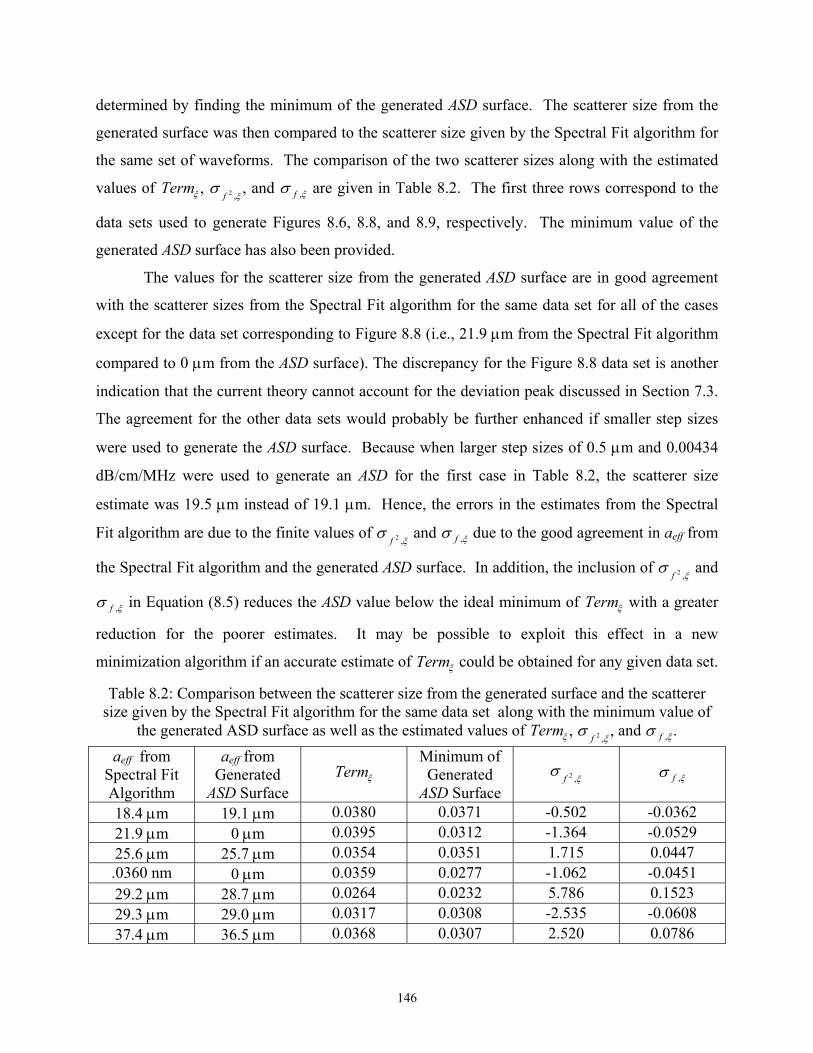
determined by finding the minimum of the generated ASD surface. The scatterer size from the
generated surface was then compared to the scatterer size given by the Spectral Fit algorithm for
the same set of waveforms. The comparison of the two scatterer sizes along with the estimated
values of Term , ξ σξf 2 ,, and σ ξ are given in Table 8.2. The first three rows correspond to the
data sets used to generate Figures 8.6, 8.8, and 8.9, respectively. The minimum value of the
generated ASD surface has also been provided.
f ,
The values for the scatterer size from the generated ASD surface are in good agreement
with the scatterer sizes from the Spectral Fit algorithm for the same data set for all of the cases
except for the data set corresponding to Figure 8.8 (i.e., 21.9 µm from the Spectral Fit algorithm
compared to 0 µm from the ASD surface). The discrepancy for the Figure 8.8 data set is another
indication that the current theory cannot account for the deviation peak discussed in Section 7.3.
The agreement for the other data sets would probably be further enhanced if smaller step sizes
were used to generate the ASD surface. Because when larger step sizes of 0.5 µm and 0.00434
dB/cm/MHz were used to generate an ASD for the first case in Table 8.2, the scatterer size
estimate was 19.5 µm instead of 19.1 µm. Hence, the errors in the estimates from the Spectral
Fit algorithm are due to the finite values of σξ and
f 2 ,σ ξ due to the good agreement in af , eff from
the Spectral Fit algorithm and the generated ASD surface. In addition, the inclusion of σξf 2 , and
σ ξf , in Equation (8.5) reduces the ASD value below the ideal minimum of Term with a greater
reduction for the poorer estimates. It may be possible to exploit this effect in a new
minimization algorithm if an accurate estimate of Term could be obtained for any given data set.
ξ
ξ
Table 8.2: Comparison between the scatterer size from the generated surface and the scatterer size given by the Spectral Fit algorithm for the same data set along with the minimum value of
the generated ASD surface as well as the estimated values of Termξ , σξ, and
f 2 ,σ ξf , .
aeff from Spectral Fit Algorithm
aeff from Generated
ASD Surface Termξ
Minimum of Generated
ASD Surface σ
ξf 2 , σ ξ f ,
18.4 µm 19.1 µm 0.0380 0.0371 -0.502 -0.0362 21.9 µm 0 µm 0.0395 0.0312 -1.364 -0.0529 25.6 µm 25.7 µm 0.0354 0.0351 1.715 0.0447 .0360 nm 0 µm 0.0359 0.0277 -1.062 -0.0451 29.2 µm 28.7 µm 0.0264 0.0232 5.786 0.1523 29.3 µm 29.0 µm 0.0317 0.0308 -2.535 -0.0608 37.4 µm 36.5 µm 0.0368 0.0307 2.520 0.0786
146
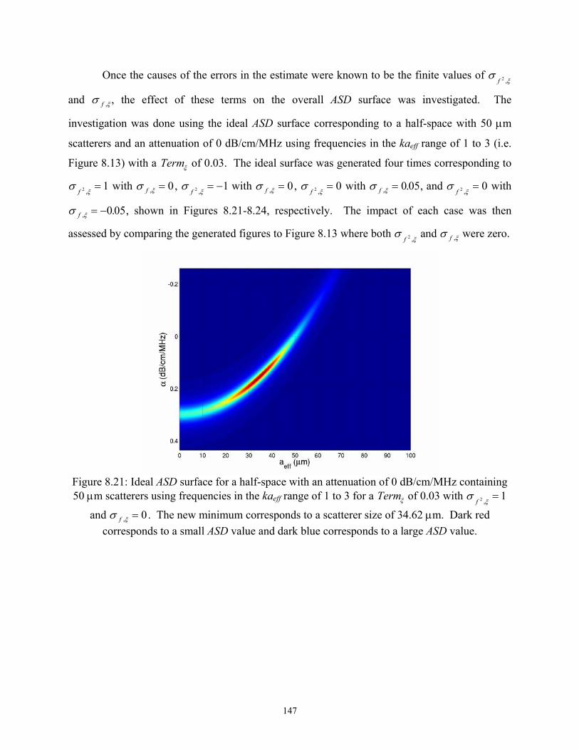
Once the causes of the errors in the estimate were known to be the finite values of σξ
and
f 2 ,
σ ξ , the effect of these terms on the overall ASD surface was investigated. The
investigation was done using the ideal ASD surface corresponding to a half-space with 50 µm
scatterers and an attenuation of 0 dB/cm/MHz using frequencies in the ka
f ,
eff range of 1 to 3 (i.e.
Figure 8.13) with a Termξ of 0.03. The ideal surface was generated four times corresponding to
σξ
1=f 2 ,
with σ ξf , = 0, σξf 2 1,
= − with σ ξf , = 0, σξf 2 0,
= with σ ξf , .= 0 05, and σξf 2 0,
= with
σ ξf , .= −0 05, shown in Figures 8.21-8.24, respectively. The impact of each case was then
assessed by comparing the generated figures to Figure 8.13 where both σξ and
f 2 ,σ ξf , were zero.
Figure 8.21: Ideal ASD surface for a half-space with an attenuation of 0 dB/cm/MHz containing 50 µm scatterers using frequencies in the kaeff range of 1 to 3 for a Termξ of 0.03 with σ
ξf 2 1,
=
and σ ξf , = 0. The new minimum corresponds to a scatterer size of 34.62 µm. Dark red corresponds to a small ASD value and dark blue corresponds to a large ASD value.
147
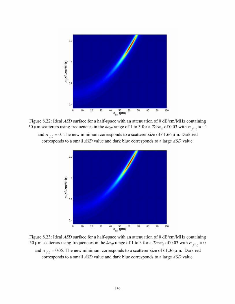
Figure 8.22: Ideal ASD surface for a half-space with an attenuation of 0 dB/cm/MHz containing 50 µm scatterers using frequencies in the kaeff range of 1 to 3 for a Term of 0.03 with ξ σ
ξf 2 1,
= −
and σ ξf , = 0. The new minimum corresponds to a scatterer size of 61.66 µm. Dark red corresponds to a small ASD value and dark blue corresponds to a large ASD value.
Figure 8.23: Ideal ASD surface for a half-space with an attenuation of 0 dB/cm/MHz containing 50 µm scatterers using frequencies in the kaeff range of 1 to 3 for a Term of 0.03 with ξ σ
ξf 2 0,
=
and σ ξf , .= 0 05. The new minimum corresponds to a scatterer size of 61.36 µm. Dark red corresponds to a small ASD value and dark blue corresponds to a large ASD value.
148

Figure 8.24: Ideal ASD surface for a half-space with an attenuation of 0 dB/cm/MHz containing 50 µm scatterers using frequencies in the kaeff range of 1 to 3 for a Term of 0.03 with ξ σ
ξf 2 0,
=
and σ ξf , .= −0 05. The new minimum corresponds to a scatterer size of 35.14 µm. Dark red corresponds to a small ASD value and dark blue corresponds to a large ASD value.
In all four figures, the parabola describing the parabolic trough occurs at the same
location and has the same width as the parabola describing the parabolic trough in Figure 8.13.
However, the minimum occurs at different locations along the trough for the different values of
σξ and
f 2 ,σ ξ . A f , σ
ξf 2 , of 1 with a σ ξ of 0 (Figure 8.21) and a f , σ
ξ of 0 with a
f 2 ,σ ξ of –0.05
(Figure 8.24) shift the minimum to a lower scatterer size and larger attenuation, while a
f ,
σξ of
with a
f 2 ,
−1 σ ξ of 0 (Figure 8.22) and a f , σξ of 0 with a
f 2 ,σ ξ of 0.05 (Figure 8.23) shift the
minimum to a larger scatterer size and smaller attenuation. Hence, for the same sign,
f ,
σξf 2 , and
σ ξf , shift the minimum in opposite directions. Because σξ and
f 2 ,σ ξ typically have the same
sign, as is indicated by the results in Table 8.2, the two frequency dependencies will
counterbalance each other. In addition, for the same magnitude of
f ,
σξ and
f 2 ,σ ξ , the shift to
smaller scatterer sizes appears to result in a larger percentage error in the new location of the
minimum. Upon examining Figure 8.13, it is clear that the ASD curve increases slightly faster as
the parabolic trough moves to larger scatterer sizes away from the minimum as opposed to
f ,
149
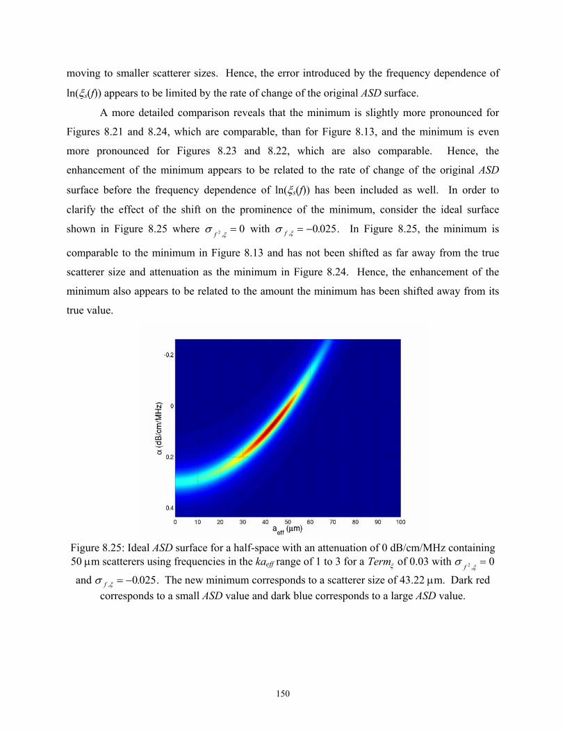
moving to smaller scatterer sizes. Hence, the error introduced by the frequency dependence of
ln(ξs(f)) appears to be limited by the rate of change of the original ASD surface.
A more detailed comparison reveals that the minimum is slightly more pronounced for
Figures 8.21 and 8.24, which are comparable, than for Figure 8.13, and the minimum is even
more pronounced for Figures 8.23 and 8.22, which are also comparable. Hence, the
enhancement of the minimum appears to be related to the rate of change of the original ASD
surface before the frequency dependence of ln(ξs(f)) has been included as well. In order to
clarify the effect of the shift on the prominence of the minimum, consider the ideal surface
shown in Figure 8.25 where σξf 2 0,
= with σ ξf , .= −0 025. In Figure 8.25, the minimum is
comparable to the minimum in Figure 8.13 and has not been shifted as far away from the true
scatterer size and attenuation as the minimum in Figure 8.24. Hence, the enhancement of the
minimum also appears to be related to the amount the minimum has been shifted away from its
true value.
Figure 8.25: Ideal ASD surface for a half-space with an attenuation of 0 dB/cm/MHz containing 50 µm scatterers using frequencies in the kaeff range of 1 to 3 for a Term of 0.03 with ξ σ
ξf 2 0,
=
and σ ξf , .= −0 025. The new minimum corresponds to a scatterer size of 43.22 µm. Dark red corresponds to a small ASD value and dark blue corresponds to a large ASD value.
150
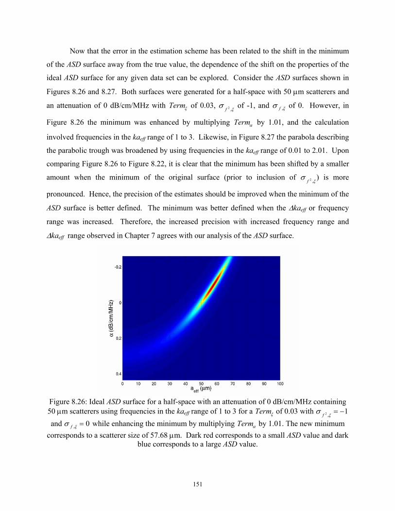
Now that the error in the estimation scheme has been related to the shift in the minimum
of the ASD surface away from the true value, the dependence of the shift on the properties of the
ideal ASD surface for any given data set can be explored. Consider the ASD surfaces shown in
Figures 8.26 and 8.27. Both surfaces were generated for a half-space with 50 µm scatterers and
an attenuation of 0 dB/cm/MHz with Termξ of 0.03, σξf 2 , of -1, and σ ξ of 0. However, in
Figure 8.26 the minimum was enhanced by multiplying Term by 1.01, and the calculation
involved frequencies in the ka
f ,
α
eff range of 1 to 3. Likewise, in Figure 8.27 the parabola describing
the parabolic trough was broadened by using frequencies in the kaeff range of 0.01 to 2.01. Upon
comparing Figure 8.26 to Figure 8.22, it is clear that the minimum has been shifted by a smaller
amount when the minimum of the original surface (prior to inclusion of σξ) is more
pronounced. Hence, the precision of the estimates should be improved when the minimum of the
ASD surface is better defined. The minimum was better defined when the ∆ka
f 2 ,
eff or frequency
range was increased. Therefore, the increased precision with increased frequency range and
∆kaeff range observed in Chapter 7 agrees with our analysis of the ASD surface.
Figure 8.26: Ideal ASD surface for a half-space with an attenuation of 0 dB/cm/MHz containing 50 µm scatterers using frequencies in the kaeff range of 1 to 3 for a Term of 0.03 with ξ σ
ξf 2 1,
= − and σ ξf , = 0 while enhancing the minimum by multiplying Term by 1.01. The new minimum
corresponds to a scatterer size of 57.68 µm. Dark red corresponds to a small ASD value and dark blue corresponds to a large ASD value.
α
151
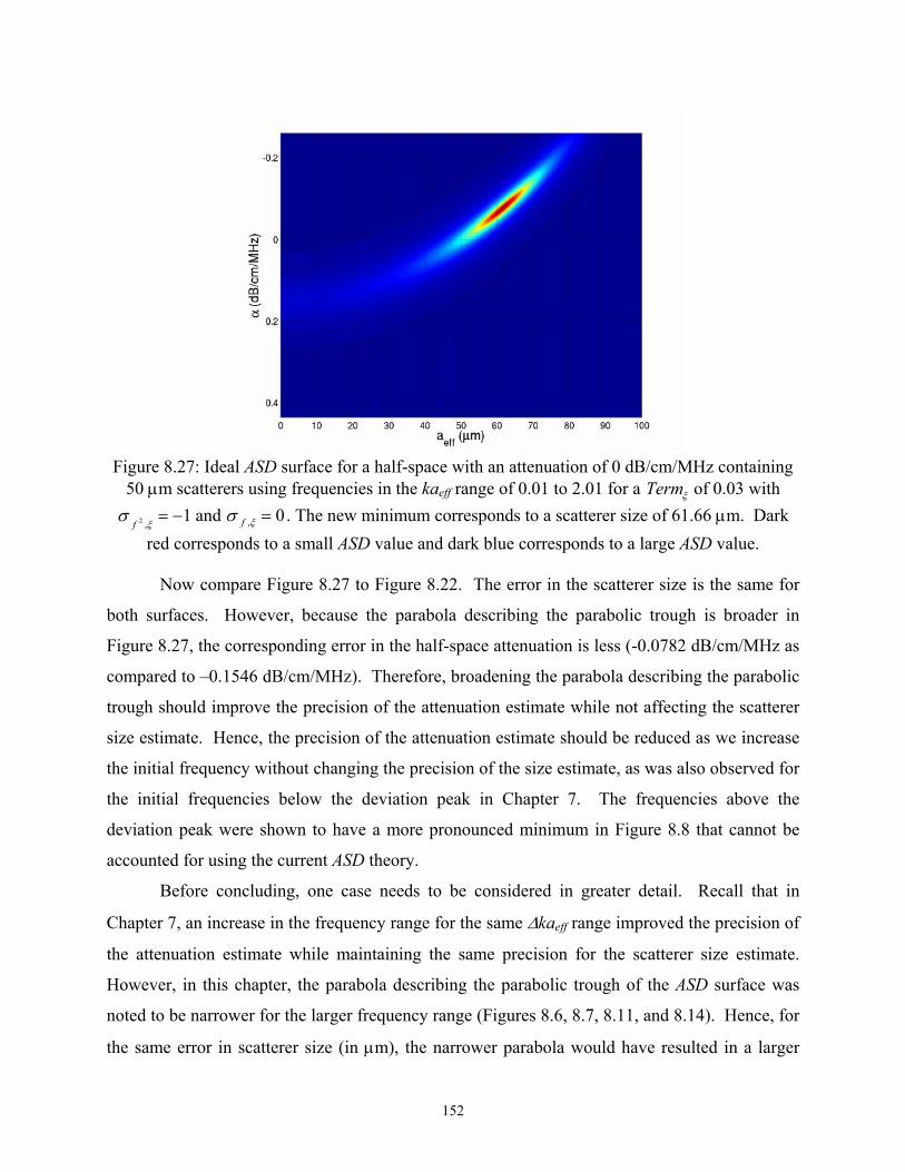
Figure 8.27: Ideal ASD surface for a half-space with an attenuation of 0 dB/cm/MHz containing
50 µm scatterers using frequencies in the kaeff range of 0.01 to 2.01 for a Termξ of 0.03 with σ
ξf 2 1,
= − and σ ξf , = 0. The new minimum corresponds to a scatterer size of 61.66 µm. Dark red corresponds to a small ASD value and dark blue corresponds to a large ASD value.
Now compare Figure 8.27 to Figure 8.22. The error in the scatterer size is the same for
both surfaces. However, because the parabola describing the parabolic trough is broader in
Figure 8.27, the corresponding error in the half-space attenuation is less (-0.0782 dB/cm/MHz as
compared to –0.1546 dB/cm/MHz). Therefore, broadening the parabola describing the parabolic
trough should improve the precision of the attenuation estimate while not affecting the scatterer
size estimate. Hence, the precision of the attenuation estimate should be reduced as we increase
the initial frequency without changing the precision of the size estimate, as was also observed for
the initial frequencies below the deviation peak in Chapter 7. The frequencies above the
deviation peak were shown to have a more pronounced minimum in Figure 8.8 that cannot be
accounted for using the current ASD theory.
Before concluding, one case needs to be considered in greater detail. Recall that in
Chapter 7, an increase in the frequency range for the same ∆kaeff range improved the precision of
the attenuation estimate while maintaining the same precision for the scatterer size estimate.
However, in this chapter, the parabola describing the parabolic trough of the ASD surface was
noted to be narrower for the larger frequency range (Figures 8.6, 8.7, 8.11, and 8.14). Hence, for
the same error in scatterer size (in µm), the narrower parabola would have resulted in a larger
152
error in the attenuation estimate. This apparent discrepancy can be reconciled by recalling that it
was the same percent error in scatterer size that resulted in the improved precision for the
attenuation estimate for the larger frequency ranges. The same percent change in scatterer size in
Figure 8.14 and Figure 8.7 still produces a larger change in the attenuation along the parabolic
trough than the corresponding percent change in Figure 8.11 and Figure 8.6. Hence, the
observations regarding the ASD surface for this case agree with the results presented in Chapter
7.
8.4 Chapter Summary
In this chapter, an analysis was performed of the ASD surface over which the Spectral Fit
algorithm finds the minimum when estimating the scatterer size and total attenuation. The
analysis was done using both the simulated waveforms from the earlier chapters as well as ideal
surfaces corresponding to a derived expression for the ASD surface. The surface was found to
have a single minimum that always occurred along a parabolic trough. The existence of the
parabolic trough could be attributed to a cross term between the attenuation and scatterer size
minimizations, Term . aeffα ,
Also, it was observed that the minimum of the ASD surface became more pronounced for
larger ∆kaeff ranges for the same frequency range (Figures 8.2, 8.3, 8.4, 8.11, and 8.13), for
larger ∆kaeff ranges for the same scatterer size (Figures 8.13 and 8.14), for the same ∆kaeff
ranges for larger frequency ranges (Figures 8.6, 8.7, 8.11, and 8.14), and for smaller spectral
variances (Figures 8.13 and 8.16). Also, the parabola describing the parabolic trough of the ASD
surface was narrowed for the same ∆kaeff range with larger frequency ranges (Figures 8.6, 8.7,
8.11, and 8.14) and for the same ∆kaeff range and frequency range with larger initial frequency
(Figures 8.6, 8.9, 8.15, and 8.11). The shift of the minimum along the parabolic trough away
from its true value was then related to the frequency dependence of the spectral variations
resulting from the random scatterer spacing, ln(ξs(f)). For the same frequency dependence of
ln(ξs(f)), the shift of the minimum away from the true value was found to be reduced
(improvement in precision) when the minimum of the surface was more pronounced. In
addition, the error in the half-space attenuation due to the shift in the minimum is less when the
parabola describing the parabolic trough is broader (all other terms remaining the same). Hence,
the analysis of the ASD surface is in agreement with the results presented in Chapter 7 regarding
153

154
∆kaeff range, frequency range, and initial frequencies below the deviation peak. The results for
initial frequencies greater than the deviation peak were found to not be consistent with ASD
analysis, once again indicating a limitation in the current theory or perhaps a simulation artifact.

CHAPTER 9
CONCLUSIONS AND FUTURE WORK
During the course of this investigation, many observations were made about the
estimation of the in vivo power spectrum as it applies to estimating the characteristic size
of the tissue microstructure. In this final chapter, the conclusions derived from all of the
observations are summarized. Then, future goals for extending the work and applying
the conclusions are discussed.
9.1 Conclusions from Current Investigation
For the estimation of the characteristic size of the tissue microstructure, the in
vivo power spectrum can be determined to sufficient accuracy by estimating the total
attenuation along the propagation path over the frequency range used to estimate the
scatterer size. Hence, most of the work in this investigation attempted to solve for the
scatterer size and total attenuation simultaneously. However, before solving for these
two parameters, the effects of focusing on the estimation of the scatterer size were
considered while assuming that the attenuation was known so that the results of the
investigation could later be applied to clinically relevant fields. By assuming that the
velocity potential fields near the focus could be modeled as a three-dimensional Gaussian
distribution, focusing could be corrected by using a new generalized attenuation-
compensation function that accounted for focusing, windowing, and attenuation.
The new generalized attenuation-compensation function was then compared to the
traditional attenuation-compensation functions that neglected focusing along the beam
axis using computer simulations and phantom experiments. The generalized attenuation-
compensation function yielded improvements in size estimation accuracy as high as
100% over the traditional attenuation-compensation functions. However, errors from the
155
choice of the attenuation-compensation function when estimating the radius of the glass
beads were much less significant than the same errors when estimating the radius of a
Gaussian scatterer due to the stronger frequency dependence of the form factor for the
glass bead scatterer. Likewise, the improvement provided by the new generalized
attenuation-compensation function decreased as the wavelength dependence of wz was
reduced. In addition, the simulations and phantom experiments had agreement better
than 2.5% provided that the same type of scatterers and sources were being compared.
After verifying the new generalized attenuation-compensation function, two
distinct algorithms for estimating the scatterer size and total attenuation simultaneously
were evaluated. For both algorithms, the evaluation was done using weakly focused
sources and relatively small window lengths so that the generalized attenuation-
compensation function could be simplified. The first algorithm was termed the Gaussian
Transformation algorithm. This algorithm estimated the scatterer size from the change in
the approximate Gaussian bandwidth and estimated the total attenuation from the
downshift in the frequency corresponding to the main spectral peak after compensating
for the scatterer size. The algorithm’s performance was reasonable for very small
attenuations, but the accuracy of the scatterer size estimate quickly degraded with
increasing attenuation. The failure was a result of the algorithm assuming that the
spectrum was perfectly Gaussian when in fact real spectra are better described by a
Rayleigh distribution that goes to zero at zero frequency.
The second algorithm evaluated did not make any assumptions about the
transmitted spectrum and was termed the Spectral Fit algorithm. The Spectral Fit
algorithm was initially tested using Gaussian scatterers with an aeff of 25 µm and using a
spectrum where the peak of the spectrum was located near 8 MHz. With this size
scatterer, the performance (i.e., accuracy and precision) of the basic Spectral Fit
algorithm was reasonable for attenuations less than 0.8 dB/cm/MHz, SNR’s for 23 dB to
28 dB, and window lengths of 8 mm. The limiting factor of the performance was a lack
of precision with increasing noise, decreasing window length, and increasing attenuation.
Hence, the rest of the investigation focused on improving the precision of the Spectral Fit
algorithm.
156
After introducing the Spectral Fit algorithm, four different signal processing
strategies were investigated with the hope of improving the precision of the Spectral Fit
algorithm. Once again, the strategies were tested using Gaussian scatterers with an aeff of
25 µm and using a spectrum where the peak of the spectrum was located near 8 MHz.
The first strategy averaged together estimates from different window lengths. Then,
homomorphic signal processing was attempted to smooth the spectra before the
minimization. The third strategy involved taking the RF echoes in different combinations
and then averaging the results together. Finally, the frequency dependence of the form
factor was varied, estimates were obtained at each assumed form factor, and a final
estimate was extrapolated from the results for each assumed form factor. In all four
cases, the signal processing did not improve the precision of the Spectral Fit algorithm.
Hence, it does not appear that robust estimates of tissue microstructure can be obtained
by new signal processing techniques alone.
When the different signal processing strategies failed to improve the precision,
different frequency ranges, ∆kaeff values, and initial frequencies were investigated by
performing simulations with different scatterer sizes, half-space attenuations, source
bandwidths, and levels of additive electronic noise. The accuracy and precision of the
attenuation estimate were consistently improved by increasing the frequency range while
the accuracy and precision of the scatterer size estimate were consistently improved by
increasing ∆kaeff. The improvement observed explained the dependence of precision on
half-space attenuation and electronic noise that was observed in the initial simulation
studies using Gaussian scatterers with an aeff of 25 µm and a spectrum where the peak
was located near 8 MHz. In addition, the Spectral Fit algorithm was shown to exhibit a
peak in the deviation of the attenuation estimate versus initial frequency that was shown
to be correlated with the frequency location of the peak in the backscattered spectrum.
The occurrence of the deviation peak may be useful in the future to improve the precision
if it is not an artifact of the simulation.
After establishing the dependence of the precision on the frequency ranges, ∆kaeff
values, and initial frequencies, the dependence was investigated further by analyzing the
average squared difference (ASD) surface (i.e., difference between backscattered
spectrum and reference spectrum modified by scatterer size and total attenuation) over
157

which the Spectral Fit algorithm finds the minimum when estimating the scatterer size
and total attenuation. The analysis was done using both the simulated waveforms as well
as ideal surfaces corresponding to a derived expression for the ASD surface. The analysis
of the ASD surface demonstrated that the precision of the estimation scheme was directly
related to the prominence of the minimum for the surface. In addition, the precision of
the attenuation estimate was related to the shape of the parabolic trough along which the
minimum always occurred. The minimum of the ASD surface became more pronounced
(better precision) for larger ∆kaeff ranges, larger frequency ranges, and smaller spectral
variances. Also, the parabola describing the parabolic trough of the ASD surface was
narrowed with larger initial frequency (poorer precision for attenuation estimate). Hence,
the analysis of the ASD surface was in agreement with the simulation results regarding
∆kaeff range, frequency range, and initial frequencies below the deviation peak. The
results for initial frequencies greater than the deviation peak were found to be
inconsistent with ASD analysis, once again indicating a limitation in the current theory or
perhaps a simulation artifact.
9.2 Future Directions for In Vivo Power Spectrum Estimation
After completing the current investigation, it was clear that there were many
aspects of the problem that needed to be investigated in more detail. More work could
certainly be done on estimating the in vivo power spectrum as it applies to estimating the
size of the tissue microstructure. In addition, the basic principles of the work could be
extended to other applications. Both types of future work are briefly discussed in this
section.
9.2.1 Future work on size estimation
Although much of the groundwork for the in vivo spectral estimation problem for
size estimation was presented in this thesis, there are many aspects that still need to be
addressed. One aspect of considerable interest is the source dependence of the
attenuation deviation peak versus initial frequency used in the estimate. Because the
current theory does not explain this peak, the first step would be to confirm that it is not
just an artifact of the simulation by performing a phantom experiment with a real
158
ultrasound source. Before the phantom experiment can be performed, however, more
simulations need to be run using glass beads (the scatterers in phantoms) instead of
Gaussian scatterers. Some of the results in Chapter 3 demonstrated that the estimation of
glass bead radii is not as affected by errors in the attenuation-compensation function.
Hence, the performance of the Spectral Fit algorithm may be slightly different, probably
improved, when using glass beads for the scatterers. As a result, the deviation peak may
not be as pronounced for these glass beads, and the simulations are required so that the
properties of the peak can be anticipated facilitating the design of the phantom
experiment.
Assuming that the existence of the deviation peak is real and not just a strange
artifact of the simulation, two other investigations should be conducted. From a
theoretical point a view, the scattering equations need to be analyzed in greater detail so
that the properties of the deviation peak can be expressed mathematically. Any
mathematical derivations would then assist in the development of a spectral coding
scheme to capitalize on the dramatic improvement in precision/accuracy after the
deviation peak. Currently, this improvement cannot be used due to the low signal levels
on this part of the backscattered spectrum.
If the deviation peak is only an artifact of the simulation, then the only definitive
way to obtain reasonable estimates of scatterer size and total attenuation simultaneously
is to use large frequency and ∆kaeff ranges. However, the bandwidth of most sources
would not allow for adequate estimates to be made using a single source. Hence,
multiple sources covering different frequency ranges would need to be used and the
resulting RF echoes combined in a single algorithm. Although multifrequency probes do
not present a manufacturing difficulty, the combination of the different RF echoes may be
difficult because the ultrasound beams from the different sources may not expose exactly
the same tissue region. Hence, the spatial resolution may be reduced because the region
exposed by all of the sources must be assumed to have the same scatterer size if the
waveforms are combined under the current theory.
In addition to the challenges associated with using multiple sources, just using
large frequency ranges on real tissue will not be trivial. First, in the work presented in
this thesis, the attenuation was always assumed to have a strict linear dependence on
159
frequency (α α= o f ) although the scatterer size estimates would still be valid when the
attenuation had a general linear dependence (α α α= +o bf ). However, in real tissue, the
attenuation has a power law dependence of the form α α= onf [Jongen et al., 1986],
where the value of n can vary from 1 to 2. Hence, a linear dependence (α α α= +o bf ) is
only valid over a limited frequency range. For larger frequency ranges, the linear
approximation would fail leading to inaccuracies in the estimate. Another challenge
related to using larger frequency ranges on real tissue is that the form factor used to
describe the tissue may only be valid over a certain range of frequencies. Recall that
Insana and Hall [1990] showed that the radius of glass beads could no longer be
estimated using the simple spherical shell form factor after a kaeff value of 1.2 due to the
influence of shear waves. A similar phenomenon may also be associated with the
scatterers in tissue. However, this cannot be determined until more is known about the
structures in tissue responsible for the scattering.
One more challenge associated with larger frequency ranges that would be a
problem even if the form factor for tissue was valid for all frequencies is the presence of
scatterers with different sizes in the same tissue region. The current investigation only
considered the estimation when a single size was present. This was done because
normally a single size in the tissue will be dominant over a certain range of frequencies.
However, if the frequency range is increased, the size estimate may be influenced by
scattering structures on a different size scale.
Clearly, there are many issues that need to be investigated before the frequency
range can be increased in real tissue experiments. However, it may be possible to
improve the precision without drastically increasing the frequency although some
increase may still be required. In this investigation, the total attenuation and scatterer
size were estimated simultaneously for every resolution cell. However, the total
attenuation should not be significantly different from one resolution cell to the next even
though the scatterer size may change. Hence, it may be possible to smooth the variations
in the attenuation estimate by averaging estimates from adjacent resolution cells
improving the precision. The averaged attenuation estimates could then be used to find
improved size estimates for each resolution cell individually. This idea needs to be tested
160

on real tissues so that the real variability in the total attenuation could be used to set the
number of resolution cells over which the attenuation estimates would be averaged.
In addition to the challenges associated with implementing and improving the
Spectral Fit algorithm, there were also some side issues that deserve further attention.
First, the Spectral Fit algorithm was only implemented using weakly focused sources.
Hence, the use of focused sources with the Spectral Fit algorithm still needs to be
investigated. Before using focused sources, however, the importance of the local
attenuation α1 in the generalized attenuation-compensation function needs to be
determined. If the local attenuation is important, then an estimation of the local
attenuation must be included in the Spectral Fit algorithm. Likewise, if errors in the local
attenuation do not affect the accuracy of the estimates for the window lengths of interest,
then the Spectral Fit algorithm can be implemented while only correcting for the focusing
along the beam axis wz as measured in a water bath. Another issue that deserves more
attention than is currently provided in the literature is the effect the scatterer number
density has on the precision of both the traditional and Spectral Fit algorithms. Lastly,
the computational efficiency of both the code used to simulate the backscattered
waveforms as well as the code used to analyze the waveforms could be improved.
9.2.2 Future work on other applications
In addition to continuing the work on predicting the in vivo power spectrum for
the purpose of estimating the characteristic size of the tissue microstructure, the method
should also be applied to other applications in the future. One application for which
some of the background work was included in the appendices of this thesis is the
estimation of the heating at the skull/brain boundary of the developing skull. In
Appendix G, the outer surface of a rat’s skull was modeled as a flat plate at some
arbitrary angle over the focal dimensions, and the effects of this assumption on estimating
the power spectrum incident on the skull were evaluated. The model was found to be
very good for a rat’s skull. However, the microstructure of the developing human skull is
very different than the fully developed rat’s skull. Hence, before the results in Appendix
G can be extended to developing humans, the RF echoes from a better animal model need
161

162
to be explored. A possible choice would be fetal pigs due to the developmental
similarities.
Another application that should be investigated is the determination of the in vivo
power spectrum to quantify ARFI measurements. In ARFI, the in vivo spectrum is
needed in order to estimate the ultrasound intensity incident on the tissue region. For
ARFI, the model would be the same as the form factor used when estimating the scatterer
size. Hence, it would be natural to combine ARFI and the quantification of the tissue
microstructure into a single measurement scheme.

REFERENCES Abbott, J.G., Rational and Derivation of MI and TI – A Review, Ultrasound in Med. & Biol., 25(3), 431-441, 1999. AIUM/NEMA, Standard for the Real-Time Display of Thermal and Mechanical Acoustic Output Indices on Diagnostic Ultrasound Equipment, Rev 1, American Institute of Ultrasound in Medicine, Laurel, MD, and National Electrical Manufacturers Association, Rosslyn, VA, 1998. AIUM, Bioeffects and Safety of Diagnostic Ultrasound, American Institute of Ultrasound in Medicine, Laurel, MD, 1993. Akita, M., and Ueda M., The effects of windowing on spectral estimation of echoes scattered by a random medium, J. Acoust. Soc. Am., 83(4), 1243-1248, 1988. Bacon, D. R., and Carstensen, E. L., Increased heating by diagnostic ultrasound due to nonlinear propagation, J. Acoust. Soc. Am., 88(1), 26-34, 1990. Barber, F. E., The scanning acoustic microprobe: I. Analysis and synthesis of a spherically symmetric point spread function, J. Acoust. Soc. Am., 90(1), 1-10, 1991. Barnett, S. B., Intracranial temperature elevation from diagnostic ultrasound, Ultrasound in Med. & Biol., 27(7), 883-888, 2001. Carlson, B. M., Human Embryology and Developmental Biology, Mosby Year Book Inc., St. Louis, MS, 1994. Cavicchi, T. J., and O’Brien, W. D., Heat generated by ultrasound in an absorbing medium, J. Acoust. Soc. Am., 76(4), 1244-1245, 1984. Cengel, Y. A., and Boles, M. A., Thermodynamics: An Engineering Approach, 2ed., McGraw-Hill, Inc., New York, 1994. Chaturvedi, P., and Insana, M. F., Error bounds on ultrasonic scatterer size estimates, J. Acoust. Soc. Am., 100(1), 392-399, 1996. Chen, J. F., Zagzebski, J. A., and Madsen, E. L., Tests of backscatter coefficient measurement using broadband pulses, IEEE Trans. Ultrason. Ferroelectr. Freq. Control, 40(5), 603-607, 1993. Chew, W. C., Waves and Fields in Inhomogeneous Media, IEEE Press, New York, 1995. Fry, W. J., and Fry, R. B., Determination of absolute sound levels and acoustic absorption coefficients by thermocouple probes – theory, J. Acoust. Soc. Am., 26(3), 294-310, 1954a.
237
Fry, W. J., and Fry, R. B., Determination of absolute sound levels and acoustic absorption coefficients by thermocouple probes – experiment, J. Acoust. Soc. Am., 26(3), 311-317, 1954b. Fujii, M., et al., Study of the cause of the temperature rise at the muscle-bone interface during ultrasound hyperthermia, IEEE Trans. Biomed. Eng., 46(5), 494-504, 1999. Gerig, A., Zagzebski, J., and Varghese, T., Statistics of ultrasonic scatterer size estimation with a reference phantom, J. Acoust. Soc. Am., 113(6), 3430-3437, 2003. Gore, J. C., and Leeman, S., Ultrasonic backscattering from human tissue: A realistic model, Phys. Med. Biol., 22(2), 317-326, 1977. Goss, S. A., Johnston, R. L., and Dunn, F., Compilation of empirical ultrasonic properties of mammalian tissues, J. Acoust. Soc. Am., 64(2), 423-457, 1978. Goss, S. A., Frizzell, L. A., and Dunn, F., Ultrasonic absorption and attenuation in mammalian tissues, Ultrasound in Med. & Biol., 5, 181-186, 1979. Goss, S. A., Johnston, R. L., and Dunn, F., Compilation of empirical ultrasonic properties of mammalian tissues. II, J. Acoust. Soc. Am., 68(1), 93-108, 1980. Goueygou, M., Harris, J. G., and O’Brien, W. D., Time-domain solution of the temperature increase induced by diagnostic ultrasound, IEEE Ultrasonics Symposium, 1385-1388, 1999. Gray, H., Gray’s Anatomy: Anatomy, Descriptive and Surgical, Courage Books, Philadelphia, PA, 1974. Haken, B. A., Frizzell, L. A., and Carstensen, E. L., Effect of mode conversion on ultrasonic heating at tissue interfaces, J. Ultrasound Med., 11, 393-405, 1992. He, P., and Greenleaf, J. F., Application of stochastic analysis to ultrasonic echoes – estimation of attenuation and tissue heterogeneity from peaks of echo envelope, J. Acoust. Soc. Am., 79(2), 526-534, 1986. Hearn, D., and Baker, M. P., Computer Graphics: C Version, 2nd ed., Prentice Hall, Upper Saddle River, New Jersey, 1997. Horder, M. M., et al., In vivo heating for the guinea-pig fetal brain by pulsed ultrasound and estimates of thermal index, Ultrasound in Med. & Biol., 24(9), 1467-1474, 1998. Insana, M. F., Madsen, E. L., Hall, T. J., and Zagzebski, J. A., Tests of the accuracy of a data reduction method for determination of acoustic backscatter coefficients, J. Acoust. Soc. Am., 79(5), 1230-1236, 1986. Insana, M. F., et al., Describing small-scale structure in random media using pulse-echo ultrasound, J. Acoust. Soc. Am., 87(1), 179-192, 1990.
238
Insana, M. F., and Hall, T. J., Parametric ultrasound imaging from backscatter coefficient measurements: Image formation and interpretation, Ultrason. Imaging, 12, 245-267, 1990. Jongen, H. A. H., et al., A general model for the absorption of ultrasound by biological tissues and experimental verification, J. Acoust. Soc. Am., 79(2), 535-540, 1986. Kakac, S., and Yener, Y., Heat Conduction, 2ed., Hemisphere Publishing Corporation, Washington, 1985. Kay, S. M. and Marple, S. L., Spectrum analysis – a modern perspective, Proceedings of the IEEE, 69(11), 1380-1419, 1981. Kino, G. S., Acoustic Waves: Devices, Imaging, and Analog Signal Processing, Prentice-Hall, Englewood Cliffs, NJ, 1987. Kudo, N., et al., Basic study on the ultrasound attenuation of fibrous biological tissue in the frequency range of 10-40 MHz, IEEE Ultrasonics Symposium, 1479-1482, 1998. Lizzi, F. L., et al., Theoretical framework for spectrum analysis in ultrasonic tissue characterization, J. Acoust. Soc. Am., 73(4), 1366-1373, 1983. Lizzi, F. L., et al., Computer model of ultrasonic hyperthermia and ablation for ocular tumors using B-mode data, Ultrasound in Med. & Biol., 18(1), 59-73, 1992. Lizzi, F. L., et al., Ultrasonic spectrum analysis for tissue assays and therapy evaluation, Int. J. Imaging Syst. Technol., 8, 3-10, 1997a. Lizzi, et al., Statistics of ultrasonic spectral parameters for prostate and liver examinations, IEEE Trans.Ultrason. Ferroelect. Freq. Contr., 44(4), 935-942, 1997b. Lubbers, J., Hekkenberg, R. T., Bezemer, R. A., Time to threshold (TT), a safety parameter for heating by diagnostic ultrasound, Ultrasound in Med. & Biol., 29(5), 755-764, 2003. Lyons, M. E., and Parker, K. J., Absorption and attenuation in soft tissues II – experimental results, IEEE Trans. Ultrason. Ferroelect. Freq. Contr., 35(4), 511-521, 1988. Madsen, E. L., Insana, M. F., and Zagzebski, J. A., Method of data reduction for accurate determination of acoustic backscatter coefficients, J. Acoust. Soc. Am., 76(3), 913-923, 1984. Madsen, E. L., et al., Interlaboratory comparison of ultrasonic backscatter, attenuation, and speed measurements, J. Ultrasound Med., 18, 615-631, 1999. Mayer, W. G., Mode conversion of ultrasonic waves at flat boundaries, IEEE Trans. Sonics. Ultrason., SU-11(1), 1-3, 1964.
239
MEDLINEplus Merriam-Webster Medical Dictionary, National Library of Medicine, 2003. Morse, P. M., and Ingard, K. U., Theoretical Acoustics, McGraw-Hill, Inc., New York, 1968. Nassiri, D. K., and Hill, C. R., The use of angular acoustic scattering measurements to estimate structural parameters of human and animal tissues, J. Acoust. Soc. Am., 79(6), 2048-2054, 1986. Narayana P. A., and Ophir J., A closed form method for the measurement of attenuation in nonlinearly dispersive media, Ultrasonic Imaging, 5, 17-21, 1983. NCRP, Exposure Criteria for Medical Diagnostic Ultrasound: I. Criteria Based on Thermal Mechanisms, NCRP Report No. 113, National Council on Radiation Protection and Measurements, Bethesda, MD, 1992. Nightingale, K. L., Nightingale, R. W., Palmer, M. L., and Trahey, G. E., A Finite Element model of remote palpation of breast lesions using radiation force: Factors affecting tissue displacement, Ultrasonic Imaging, 22, 35-54, 2000. Nishimura, H., et al., Prenatal Development of the Human with Special Refrence to Craniofacial Structures: An Atlas, US Dept. of Health, Education, and Welfare, Bethesda, ML, 1977. Nyborg, W. L., Heat generation by ultrasound in a relaxing medium, J. Acoust. Soc. Am., 70(2), 310-312, 1981. O’Brien, W. D., Ultrasonic Techniques, Class Notes for ECE374, Department of Electrical and Computer Engineering, University of Illinois at Urbana-Champaign, 2000. O’Donnell, M., and Miller, J. G., Quantitative broadband ultrasonic backscatter: An approach to nondestructive evaluation in acoustically inhomogeneous materials, J. Appl. Phys., 52(2), 1056-1064, 1981. Oelze, M. L., and O’Brien, W. D., Jr., Frequency-dependent attenuation-compensation functions for ultrasonic signals backscattered from random media, J. Acoust. Soc. Am., 111(5), 2308-2319, 2002a. Oelze, M. L., and O’Brien, W. D., Jr., Method of improved scatterer size estimation and application to parametric imaging using ultrasound, J. Acoust. Soc. Am., 112(6), 3053-3063, 2002b. Oelze, M. L., Zachary, J. F., and O’Brien, W. D., Characterization of tissue microstructure using ultrasonic backscatter: theory and technique optimization using a Gaussian form factor, J. Acoust. Soc. Am., 112(3), 1202-1211, 2002. Ohtuski, F., Developmental changes of the cranial bone thickness in the human fetal period, Am. J. Phys. Anthrop., 46, 141-154, 1977.
240
Parker, K. J., The thermal pulse decay technique for measuring ultrasonic absorption coefficients, J. Acoust. Soc. Am., 74(5), 1356-1361, 1983. Parker, K. J., Effects of heat conduction and sample size on ultrasonic absorption measurements, J. Acoust. Soc. Am., 77(2), 719-725, 1985. Paulsen, K. D., Hoopes, J. P., and Ryan, T. P., Is penile electrocautery safe? Part II: Temperature assessment in a pediatric computational model, Thermal Treatment of Tissue: Energy Delivery and Assessment, Proc. of SPIE, 4247, 194-202, 2001. Peebles, P. Z., Probability, Random Variables, and Random Signal Principles, 3rd ed., McGraw-Hill, Inc., New York, 1993. Pennes, H. H., Analysis of tissue and arterial blood temperatures in the resting human forearm, J. of Appl. Physiol., 1(2), 93-122, 1948. Pierce, A. D., Acoustics: An Introduction to Its Physical Principles and Applications, Acoustical Society of America, Woodbury, New York, 1991. Proakis, J. G., and Manolakis, D. G., Digital Signal Processing: Principles, Algorithms, and Applications, 3rd ed., Prentice Hall, Upper Saddle River, New Jersey, 1996. Raum, K., and O’Brien, W. D., Pulse-echo field distribution measurement technique for high-frequency ultrasound sources, IEEE Trans. Ultrason. Ferroelectr. Freq. Control, 44(4), 810-815, 1997. Routh, H. F., Doppler ultrasound: The ability to measure and image blood flow, IEEE Eng. Med. Biol., November/December, 31-40, 1996. Siddiqi, T. A., Miodovnik, M., Meyer, R. A., and O’Brien, W. D., Jr., In vivo ultrasonographic exposimetry: Human tissue-specific attenuation coefficients in the gynecologic examination, Am. J. Obstet Gynecol., April, 866-874,1999. Sidney, D. A., Three-dimensional ultrasound power deposition modeling, thermal field visualization, and clinical integration for hyperthermia therapy, PhD dissertation, Massachusetts Institute of Technology, 1997. Simpson, D. H., Burns, P. N., and Averkiou, M. A., Techniques for perfusion imaging with microbubble contrast agents, IEEE Trans. Ultrason. Ferroelect. Freq. Contr., 48(6), 1483-1494, 2001. Wear, K. A., et al., Differentiation between acutely ischemic myocardium and zones of completed infarction in dogs on the basis of frequency-dependent backscatter, J. Acoust. Soc. Am., 85(6), 2634-2641, 1989.
241
242
Wear, K. A., Ultrasonic attenuation in human calcaneus from 0.2 to 1.7 MHz, IEEE Trans. Ultrason. Ferroelect. Freq. Contr., 48(2), 602-608, 2001a. Wear, K. A., Fundamental precision limitations for measurements of frequency dependence of backscatter: Applications in tissue mimicking phantoms and trabecular bone, J. Acoust. Soc. Am., 110(6), 3275-3282, 2001b. Wear, K. A., A Gaussian framework for modeling effects of frequency-dependent attenuation, frequency-dependent scattering, and gating, IEEE Trans. Ultrason. Ferroelectr. Freq. Control, 49(11), 1572-1582, 2002. Wilkening, W., et al., Brain perfusion imaging using contrast agent specific imaging modes, IEEE Ultrason. Symp., 1721-1724, 1999. Wilkening, W., et al., Ultrasonic assessment of perfusion conditions in the brain and in the liver, IEEE Ultrason. Symp., 1545-1548, 2000. Wojcik, J., Filipczynski, L., and Kujawska, T., Temperature elevations computed for three-layer and four-layer obstetrical tissue models in nonlinear and linear ultrasonic propagation cases, Ultrasound in Med. & Biol., 25(2), 259-267, 1999.
APPENDIX A: REVIEW OF THERMODYNAMICS
This appendix contains a brief review of thermodynamic terminology and the 1st Law of
Thermodynamics. Often, the fields of acoustics and thermodynamics are studied by different
people. As a result, the two disciplines develop different methods of describing the same
phenomenon. In this appendix, the basic principles of thermodynamics will be restated in an
acoustics framework to enhance further derivations.
Review of Basic Terms:
Before discussing the laws governing thermodynamics, it is necessary to review the
terminology used to describe the basic physics involved. When discussing thermodynamics, one
often speaks of the state of the medium [Cengel and Boles, 1994]. The state refers to a unique
set of properties that capture the behavior of the molecules of interest [Cengel and Boles, 1994].
The properties can either be intensive, independent of the size of the medium being considered
(i.e., temperature, pressure, entropy, and density), or extensive, dependent on the size of the
medium (i.e., mass and volume) [Cengel and Boles, 1994]. However, the complete
thermodynamic state is known once any two independent intensive properties of the material
have been specified provided that the region of interest is a simple compressible system [Cengel
and Boles, 1994]. A simple compressible system exists whenever electric, magnetic,
gravitational, motion, and surface tension effects can be ignored [Cengel and Boles, 1994].
Hence, acoustics almost always deals with simple compressible systems with the only exception
being surface tension effects at the boundary of gas/fluid media [Pierce, 1991].
Given these concepts, thermodynamics is nothing more than the study of how a material
changes from one thermodynamic state to another. When all of the molecules in a particular
region have the same properties, the region is said to be in thermodynamic equilibrium [Cengel
and Boles, 1994]. A region must be in equilibrium before the state can be specified by its
intensive properties. However, it would be convenient if the properties could also be used to
describe the intermediate states when the system is in transition. Therefore, it is often assumed
that the transition between thermodynamic states is slow enough so that all of the molecules in a
region of interest have the same properties at all times. Such a transition is called a quasi-
163
equilibrium process [Cengel and Boles, 1994]. In acoustics, this would mean that the frequency
of the sound propagation must be less than some threshold value [Pierce, 1991]. The properties
of a material undergoing a quasi-equilibrium process change according to the material’s equation
of state [Cengel and Boles, 1994]. The equation of state governs the relationship between the
different properties. The most common equation of state is the ideal gas law [Cengel and Boles,
1994]. For most materials, however, the equation of state is too complicated to be found
empirically.
There are two thermodynamic state transitions that are of importance in the study of
acoustics: isothermal changes and adiabatic changes. Under isothermal conditions, the
temperature of the region of interest remains constant over time [Cengel and Boles, 1994]. Heat
may flow, but this change in energy would be expressed by changes in the thermodynamic
properties other than temperature. For an adiabatic process, however, there is no heat flow
[Cengel and Boles, 1994]. Because heat flow is driven by temperature differentials between a
region and its surroundings, this would mean that either all regions of a medium have the same
temperature at all times, or that a region is completely insulated from its surroundings [Cengel
and Boles, 1994]. Furthermore, because the specific entropy of a region can only be changed by
heat or mass flow, an adiabatic process acting on a region in the absence of mass flow would
result in constant entropy over time. In either case, if one of the properties of a system is
constant over time, then the complete thermodynamic state can be completely specified by only
one intensive property.
In the field of acoustics, the study of changes in the thermodynamic state of the medium
is generally expressed in terms of changes in the intensive properties of a fluid particle [Pierce,
1991]. A fluid particle is an arbitrary clump of molecules in the same quasi-equilibrium
thermodynamic state that move together in the medium. As a result, the total mass of the fluid
particle would remain constant over time and there would be no mass flow. As a result, the fluid
particle would be considered a control mass or closed system in thermodynamics [Cengel and
Boles, 1994]. However, because the density of the particle would be changed by the acoustic
disturbance, the total volume of the fluid particle would vary over time.
The other, more general, type of system in thermodynamics is the control volume or open
system [Cengel and Boles, 1994]. However, some authors, such as Kakac and Yener [1985],
restrict the use of the term “system” to only refer to closed systems. The control volume is a
164
selected region that allows both mass flow in and out of the region as well as for changes in the
region’s volume [Cengel and Boles, 1994; Kakac and Yener, 1985]. In effect, the control mass
would just be a special case of the control volume. The most common special case, however, is
when the volume of the region is fixed, the dual of the control mass, and is commonly what is
meant by the term “control volume” [Cengel and Boles, 1994].
First Law of Thermodynamics
The first law of thermodynamics is nothing more than the conservation of energy [Cengel
and Boles, 1994]. Often, however, it is convenient to specify the law in terms of the time rate of
change of the energy rather than the total energy present. In this form, the first law for thermo-
mechanical interactions is given as
dEdt
Q Q Wi e= + + , (A.1)
where E is the total energy in the system, is the rate heat is generated or removed internally,
is the rate heat flows into the system, and W is the rate work interacts with the system. If we
restrict our attention to a single fluid particle, Equation (A.1) can be rewritten as
iQ
eQ
∂∂
⋅ + + +FHG
IKJ
= − ⋅ + ⋅
=
=
∑zzzzzz zz ∑zz
tu u e S dV
q dV q ndS u e ndS
L d ij d i L ij d ii jV
iV S
ij i ji jS
12
12
21
3
1
3
ρ ρ λ θ δ ξ µ ξ
σ
d i,
,
*
* * *
, (A.2)
where the total energy term has been expanded to include both the kinetic energy of the moving
molecules, the thermodynamic internal energy e, and the stored elastic energy for an isotropic
medium. The elastic energy term involves the Lame’ constants λL and µL, the dilatation θd, the
strain tensor S, and the displacement ξ d . Gravitational potential energy has been ignored
because this quantity is in general not time varying for acoustic problems. In this equation, q is
the heat generated within the particle,
i
q is the heat flow across the boundary of the particle, and
σ is a tensor representing the external forces acting on the fluid particle. The other parameters in
Equation (A.2) are defined as the outward unit normal for the particle , the velocity n u , and the
density ρ.
165
APPENDIX B: OVERVIEW OF HUMAN SKULL
This appendix contains a brief review of the development of the fetal skull. The goal is
to provide a qualitative understanding of the location and ossification process of the principle
features of the developing skull.
Anatomical Features of the Skull
The skull consists of many different bones, each engineered to provide support and allow
for growth of the developing baby both before and after birth. These bones can be roughly
divided into two major subdivisions which are the neurocranium and the viscerocranium
[Carlson, 1994]. The neurocranium consists of the bones that surround and protect the brain and
brain stem, whereas the viscerocranium surrounds the oral cavity, pharynx, and upper respiratory
passages [Carlson, 1994]. Hence, for the purpose of heat related bioeffects on the developing
fetal brain, only the neurocranium is of importance.
The major bones of the neurocranium are the frontal bone, the parietal bones, the
occipital bone, the sphenoid bones, and parts of the temporal bones [Carlson, 1994]. The frontal
bone extends approximately from the eye sockets to the top of the head and spans from one
temple to the other as shown in Figure B.1. At birth, the frontal bone is divided into two halves
separated by a suture [Gray, 1974] and has a typical thickness at the ossification centers of 396
µm [Ohtsuki, 1977]. A suture is a gap between the skull bones that allows the brain cavity to
continue to grow, which will later fill in after growth has competed. In Figure B.1, additional
sutures are shown as lines separating the bones. Behind the frontal bone are the two parietal
bones which extend over most the top and sides of the skull [Gray, 1974]. At birth, a typical
thickness for a parietal bone at the ossification center is 543 µm [Ohtsuki, 1977]. After the
parietal bones, there is the occipital bone at the base of the skull that covers the transition from
the cerebrum to the cerebellum protecting the brain stem [Gray, 1974]. At birth, the occipital
bone consists of four separate parts that are later joined [Gray, 1974] and has a typical thickness
at the ossification center of 1654 µm [Ohtsuki, 1977]. On either side of the head, there are the
sphenoid bones and the temporal bones adjacent to the parietal bones, frontal bone, and the
166

viscerocranium as shown in Figure B.1. At birth, the temporal bone has a typical thickness of
328 µm at its midpoint [Ohtsuki, 1977].
Figure B.1: Diagram showing position of important skull bones. [Modified from MEDLINEplus
Merriam-Webster Medical Dictionary, National Library of Medicine, 2003]
Ossification of the Skull
In addition to the anatomical subdivision of the skull bones in terms of neurocranium and
viscerocranium, the bones can also be classified in terms of how the ossification is accomplished.
In one case, the “bones” begin as cartilage which is gradually replaced by bone [Carlson, 1994].
This is the same process by which bones in the limbs are formed. In the skull, most of the
occipital bone, the sphenoid bones, and parts of the temporal bones are ossified by this process
[Carlson, 1994].
The second method of ossification involves the direct formation of bone without the
cartilage intermediate step [Carlson, 1994]. In the skull, the parietal bones, frontal bone, a small
part of the occipital bones, and the rest of the temporal bones are ossified by this process
[Carlson, 1994]. For this method, the ossification begins near the center of the bone and
proceeds along branching tubules until the bone plate has filled in [Nishimura et al., 1977].
167

APPENDIX C: DERIVATION OF THE BIOHEAT EQUATION
For many years, there has been considerable interest in the propagation of temperature
variations in the human body. This interest has been spawned by the large number of biological
effects that are related to temperature changes in tissue. The earliest development was given by
Pennes [1948] in his study of blood temperatures in the resting human forearm. In his article,
Pennes provided a differential equation, the bioheat equation, that could be used to calculate
temperature distributions in the human body based on thermal conduction. Pennes assumed that
the medium was thermally homogeneous in order to obtain a tractable problem.
Due to modern computational power, however, the homogeneous tissue assumption is no
longer required. Therefore, in this appendix, the complete bioheat equation will be derived from
the basic principles of energy conservation. The derivation in the first section is similar to that
provided by Kakac and Yener [1985] in that the substance is assumed to be incompressible and
no work is being done on the fluid particles. After completing this derivation, the results are
generalized to include both compressible materials as well as materials undergoing work related
interactions. Finally, the effect of relaxation processes and elasticity in an isotropic medium are
considered due to their importance in biological materials.
Heat Conduction in Incompressible Substance without Work Acting on System:
The first step in deriving the bioheat equation is to temporarily assume that the medium
of interest is incompressible, density constant with respect to time, and that no work is being
done on any of the fluid particles. Because the density is an intensive property, this means that
the state of the system is uniquely determined by only one other intensive property (i.e., p =
p(T)). As a result, the pressure p must be a function of time and space because the temperature
distribution should also be a function of time and space. Hence, in order not to have any work
acting on the system, the particle velocity u and the particle displacement must also be zero.
Hence, the energy conservation equation given in Appendix A simplifies to yield
ξ d
168

∂∂
= − ⋅
⇒ − + ∇ ⋅FHG
IKJ =
⇒∂∂
+ ⋅∇FHG
IKJ − + ∇ ⋅
FHG
IKJ =
⇒∂∂
− + ∇ ⋅ =
zzz zzz zzzzzzzz
tedV q dV q ndS
DeDt
q q dV
et
u e q q dV
et
q q
Vi
V S
iV
iV
i
ρ
ρ
ρ
ρ
* * *
*
*
,
0
0
0
b g (C.1)
where e is the thermodynamic internal energy, ρ is the density, q is the contribution of any heat
sources/sinks in the medium, and q is the heat flow due to thermal conduction.
i
In order to complete the derivation of the bioheat equation for this special case, use is
made of Fourier’s Law of heat conduction (i.e., q Tt= − ∇κ where κt is the thermal conductivity
of the medium, and T is the temperature) and the thermodynamic relationship e = e(T) resulting
from the incompressibility of the medium. Applying basic principles of differential equations
then yields
de eT
dT c dT
et
c Tt
V
V
=∂∂
=
⇒∂∂
=∂∂
, (C.2)
where cV is the specific heat at constant volume. As a result, Equation (C.1) becomes
ρc κTt
qV i t T∂∂
= + ∇ ⋅ ∇ (C.3)
which is the general heat conduction equation. The bioheat equation is formed by simply
separating the q into a heat source term and a blood perfusion term as shown in Equation (C.4)
[Pennes, 1948]. i
ρc κTt
q qV blood source t T∂∂
= + + ∇ ⋅ ∇ (C.4)
Heat Conduction in Compressible Substance without Work Acting on System:
The previous analysis was restricted to incompressible substances. However, in general,
the material will be compressible, so the question remains as to whether the bioheat equation
would still apply. Once again, u must be zero in order to avoid work done by shearing forces.
As a result, the only change in the previous analysis pertains to writing the change in internal
169

energy e as a function of a change in the temperature T in Equation (C.2). Therefore, Equation
(C.2) becomes
de e d c dT
et
et
c Tt
TV
TV
=∂∂FHGIKJ +
⇒∂∂
=∂∂FHGIKJ
∂∂
+∂∂
ρρ
ρρ .
(C.5)
Furthermore, applying the conservation of mass [Pierce, 1991] yields
∂∂
= −∇ ⋅ = ⇒∂∂
=∂∂
ρ ρt
u et
c TtVb g 0 (C.6)
because u is zero. Therefore, the bioheat equation would be exactly the same for a compressible
material as for an incompressible material.
Heat Conduction in Compressible Substance with Work Acting on System:
For many heat conduction problems, the analysis up to this point would suffice because
there is no mechanical work acting on the fluid particles. For example, heating due to
electromagnetic exposure as was done by Paulsen et al. [2001] can be accurately characterized.
Unfortunately, when dealing with heating due to ultrasound, the mechanical interactions of the
fluid particles can no longer be ignored (i.e., u ≠ 0). Therefore, it is necessary to return to the
energy conservation equation to determine if another heat conduction equation could be found
for this case by separating the thermal and the mechanical effects. During this derivation, all
thermodynamic processes will be assumed to be in quasi-equilibrium and elastic forces will be
assumed negligible. Relaxation and elastic effects will be considered after this initial analysis is
complete.
The conservation of energy equation for a viscous medium neglecting elasticity is given
by
∂∂
⋅ +FHG
IKJ = − ⋅ + ⋅ + ⋅zzz zzz zz zz ∑zz
=tu u e dV q dV q ndS u ndS u e ndS
Vi
V Sn
Sij i j
i jS
12 1
3
ρ ρ σ µ φ* * * * * ,
(C.7)
where σn is the average of the normal components of the stress tensor and µ is the shear viscosity
[Pierce, 1991]. For a simple viscous medium, σn is just the negative of the pressure p [Pierce,
1991]. The first step in separating the thermal and mechanical effects is to make use of the
thermodynamic identity [Cengel and Boles, 1994]
170
de c dT T pT
p dV= +∂∂FHGIKJ −
LNMM
OQPP
−
ρ
ρ 1. (C.8)
Substituting this value for the internal energy into Equation (C.7) yields
12
1
1
3
ρ ρ ρ ρ
µ φ
ρ
DDt
u u c DTDt
T pT
p DDt
dV
q dV q ndS pu ndS u e ndS
VV
iV S S
ij i ji jS
⋅ + +∂∂FHGIKJ −
LNMM
OQPP
FHG
IKJ
= − ⋅ − ⋅ + ⋅
−
=
zzzzzz zz zz ∑zzb g
*
* * * *
.,
(C.9)
Now, transform this equation into an equation involving small perturbations about the ambient
state by assuming
p p pT T T
u u
o
c
c
= + ′= + ′= + ′= ′
ρ ρ ρ.
(C.10)
These values can be substituted into Equation (C.9) to yield
ρ ρρ
ρρ
ρ
κ µ φ
κ
ρ ρ21 1
1
3
DDt
u u c DTDt
T pT
p DDt
T pT
p DDt
dV
q T dV u e ndS p p u dV
q T p u dV
V cV
i tV
ij i ji jS
oV
i tV
⋅ +′− ′
∂∂ oFHGIKJ − ′
LNMM
OQPP
−∂∂FHGIKJ −
LNMM
OQPP
FHG
IKJ
= +∇⋅ ∇ ′ + ⋅FHG
IKJ − ∇⋅ + ′
= +∇⋅ ∇ ′ −∇⋅ ′
zzzzzz ∑zz zzz
=
b g
b g b gc h
b gc h
*
* * *
*
,
zzz ∑zz zzzzzz ∑zz zzz
+ ⋅FHG
IKJ − ∇⋅
= +∇⋅ ∇ ′ −∇⋅ ′ + ⋅FHG
IKJ +
=
=
µ φ
κ µ φρ
ρ
ij i ji jS
oV
i tV
ij i ji jS
o
V
u e ndS p udV
q T p u dV u e ndS p DDt
dV ,
,
,
* *
* * *
1
3
1
3
b gc h
(C.11)
where the conservation of mass equation [Pierce, 1991] has been manipulated to yield
0
1
1
= ∇ ⋅ +∂∂
⇒ −∂∂
= ⋅∇ + ∇ ⋅
⇒ ∇ ⋅ = −∂∂
+ ⋅∇FHG
IKJ
⇒∇⋅ = −
ρ ρ ρ ρ ρ
ρρ ρ
ρρ
ut t
u u
ut
u
u DDt
b g
.
(C.12)
Therefore, Equation (C.11) becomes
171

12
1
1
3
ρ ρρ
ρρ
ρ
κ µ φ
ρ ρ
DDt
u u c DTDt
T pT
p DDt
T pT
DDt
dV
q T p u dV u e ndS
Vc
V
i tV
ij i ji jS
⋅ +′− ′
∂∂FHGIKJ − ′
LNMM
OQPP
−∂∂FHGIKJ
FHG
IKJ
= + ∇ ⋅ ∇ ′ − ∇ ⋅ ′ + ⋅FHG
IKJ
zzzzzz ∑zz
=
b g
b gc h
*
* *
.,
(C.13)
Applying
dp pT
dT p d
p pT
T c
T
T
=∂∂FHGIKJ +
∂∂FHGIKJ
⇒ ′ =∂∂FHGIKJ ′ + ′
ρ
ρ
ρρ
ρ2
(C.14)
then yields
12
2
2
1
3
ρ ρρρ
ρρ
ρ
κ ρ µ
ρ
ρ
DDt
u u c DTDt
c DDt
dVT p
TDDt
dV
q T u pT
T c dV u e ndS
VT
V
c
V
i t TV
ij i ji jS
⋅ +′+
′
φ
FHG
IKJ −
∂∂FHGIKJ
FHG
IKJ
= + ∇ ⋅ ∇ ′ − ∇ ⋅∂∂FHGIKJ ′ + ′
LNMM
OQPP
FHG
IKJ
FHG
IKJ
+ ⋅FHGG
IKJJ
zzz zzzzzz ∑zz
=
b g* *
* *
,,
(C.15)
where cT is speed of sound assuming isothermal propagation. Also,
∂∂FHGIKJ = −
∂∂FHGIKJ
∂∂FHGIKJ =
pT
pT
cT p
T thermρ ρ
ρ ρ β2 , (C.16)
where βtherm is the coefficient of thermal expansion [Pierce, 1991] leaving
12
22
2 2
1
3
ρ ρρρ
ρ β ρ
κ ρ β ρ µ φ
DDt
u u c DTDt
c DDt
dV T c DDt
dV
q T u c T c dV u e n
VT
Vc T therm
V
i t T therm TV
ij i ji jS
⋅ +′+
′FHG
IKJ − FHG
IKJ
= + ∇ ⋅ ∇ ′ − ∇ ⋅ ′ + ′ + ⋅FHG
IKJ
zzz zzzzzz ∑zz
=
b g
e je j
* *
* *
.,
dS
(C.17)
Because only the first-order perturbations in the energy are of interrest, only the lowest
order terms are retained. This would be terms containing only ′T or terms that are second order
in the other variables. Therefore, terms like uT ′ would be eliminated because it is not of the
lowest order. This yields
12
22
2
1
3
ρ ρ ρρ
ρ β ρ
κ ρ µ φ
c c VT
cVc T therm
V
i t TV
ij i ji jS
tu u c T
tc
tdV T c
tdV
q T uc dV u e ndS
∂∂
⋅ +∂ ′∂
+′ ∂ ′∂
FHG
IKJ −
∂ ′∂
FHG
IKJ
= +∇⋅ ∇ ′ −∇⋅ ′ + ⋅FHG
IKJ
zzz zzzzzz ∑zz
=
b g
c he j
* *
* *
.,
(C.18)
172
Now, if the ratio of the specific heats is very close to one, as is the case for biological
tissue, Equation (C.18) becomes
12
12 2
2
1
3
ρρ
µφ β
κ ρ
cc T
ij i ji j
c therm
i t c V
tu u up
cpt
u e T pt
q T c Tt
∂∂
⋅ +∇⋅ ′ +∂ ′∂
−∇⋅FHG
IKJ −
∂ ′∂
=
+∇⋅ ∇ ′ −∂ ′∂
=∑b g b g
.
, (C.19)
Furthermore, the Tcβtherm term can also be neglected if its order is compared to the pressure
squared term. Tc thermβ ~ . .300 88 10 0 02645⋅ ⋅ =− , but the pressure squared term is of order
ωρ
π′⋅
pcc T2
1010002 ~ ⋅ ⋅
=500 101487
7106 3
2 when the frequency is in the megahertz range and the pressure is
at least 500 kPa. Hence, Equation (C.19) can be written as
∂∂
+∇⋅ ′ = +∇⋅ ∇ ′ −∂ ′∂
wt
I q T c Tti t c Vκ ρ , (C.20)
where
wu u p
c
I up u e
o
c T
ij i ji j
=⋅
+′
′ = ′ −=∑
ρρ
µφ
b g2 2
2
2
1
3
.,
(C.21)
Equation (C.20) is very close to the previously derived bioheat equation with the left-
hand side acting as an additional heat source. More will be said about the left-hand side after
elastic and relaxation effects have been included.
Heat Conduction in an Elastic System with Relaxation Processes
In the previous section, the expressions for heat conduction in a simple viscous medium
were developed. However, biological tissues are affected by relaxation processes and elastic
forces that affect the conservation of energy in the thermal-mechanical interactions. As a result,
the complete energy conservation equation provided in Appendix A will need to be considered.
For convenience, the equation is restated below:
∂∂
⋅ + + +FHG
IKJ
= − ⋅ + ⋅
=
=
∑zzzzzz zz ∑zz
tu u e S dV
q dV q ndS u e ndS
L d ij d i L ij d ii jV
iV S
ij i ji jS
12
12
21
3
1
3
ρ ρ λ θ δ ξ µ ξ
σ
d i,
,
*
* * *
. (C.22)
173
In this equation, q is the heat generated within the particle, i q is the heat flow across the
boundary of the particle, and σ is a tensor representing the external forces acting on the fluid
particle. For an isotropic viscous relaxing elastic medium, σ is given by [O’Brien, 2000]
σ λ θ δ µ µ θ δ µij L d ij L ij B d ij ijS= S+ + +2 2 (C.23)
whose parameters are the Lame’ constants λL and µL, the bulk and shear viscosity µB and µ, the
dilatation θd, and the tensor strain S. The other parameters in Equation (C.22) are defined as the
outward unit normal for the particle , the velocity n u , the displacement ξ d , and the density ρ.
Now separate out the temperature from the internal energy similar to the previous cases.
A discussion of internal energy with relaxation effects included can be found in Pierce [1991];
however, for this derivation the following relation will be sufficient:
de Tds pd A dT= − −− ∑ρ ν νν
1 . (C.24)
In this equation, s is the entropy, and the summation captures the energies of the vibrational
motions of the molecules. Substituting this equation into the energy conservation equation yields
12
221
3
1
3
DDt
SD u u
DtT Ds
Dtp D
DtA DT
DtdV
q dV q ndS u e ndS
L d ij d i L ij d ii jV
iV S
ij i ji jS
λ θ δ ξ µ ξ ρ ρρ
ρ ρ
σ
νν
ν
+ +⋅
+ + −FHG
IKJ
= − ⋅ + ⋅
=
=
∑ ∑zzzzzz zz ∑zzd i b g
,
,
*
* * *
.(C.25)
Now decompose the entropy into two distinct contributions sfr and sν [Pierce, 1991]:
s s sfr= +∑ νν
. (C.26)
In this equation, sfr corresponds to the entropy associated with translational and rotational
motions of the fluid particles, and sν captures the entropy associated with the much smaller
vibrational motions. The subscript fr refers to a frozen state where molecules are not allowed to
vibrate, and the subscript ν refers to the different possible vibrational modes for the molecules.
Then from thermodynamics [Pierce, 1991]
dsT
decT
dTvν
νν
ν
ν
= =1
ν (C.27)
and [Cengel and Boles, 1994]
174
dssT
dTs
d
dscT
dTsp
p d
dscT
dTsp
c d
frfr fr
T
frVfr fr
T T
frVfr fr
TT
=∂
∂FHGIKJ +
∂
∂FHGIKJ
⇒ = +∂
∂FHGIKJ
∂∂FHGIKJ
⇒ = +∂
∂FHGIKJ
ρρ
ρ
ρρ
ρ2 ,
(C.28)
where the thermodynamic quantities are those appropriate for the frozen state. Applying the
Maxwell relation [Cengel and Boles, 1994]
∂
∂FHGIKJ = −
∂∂FHGIKJ
−sp Tfr
T p
ρ 1
(C.29)
then yields
dscT
dTT
c d
dscT
dT c d
frVfr
pT
frVfr therm
T
= −∂∂FHGIKJ
⇒ = −
−ρ ρ
βρ
ρ
12
2 .
(C.30)
Substituting Equations (C.26), (C.27), and (C.30) into Equation (C.25) then yields
12
221
3
2
1
3
DDt
SD u u
Dtc DT
Dt
p T c DDt
TcT
DTDt
ADTDt
dV
q dV q ndS u e ndS
L d ij d i L ij d ii j
Vfr
therm TvV
iV S
ij i ji jS
λ θ δ ξ µ ξ ρ ρ
ρβ ρ ρ
ρ
σ
ν
ν
ν
νν
ν
ν
+ +⋅
+
+ −FHG
IKJ + −
F
H
GGGG
I
K
JJJJ
= − ⋅ + ⋅
=
=
∑
∑ ∑zzz
zzz zz ∑zz
d i b g,
,
*
* * *
.
(C.31)
Equation (C.31) can be further simplified by the relation [Pierce, 1991]
ρ ρνν
νν
ν
ν
ν
ADTDt
c TT
DTDtv∑ ∑= −
FHGIKJ1 (C.32)
to yield
12
221
3
2
1
3
DDt
SD u u
Dtc DT
Dt
p T c DDt
cDTDt
dV
q dV q ndS u e ndS
L d ij d i L ij d ii j
Vfr
therm T vV
iV S
ij i ji jS
λ θ δ ξ µ ξ ρ ρ
ρβ ρ ρ
σ
νν
ν
+ +⋅
+
+ −FHG
IKJ +
F
H
GGGG
I
K
JJJJ
= − ⋅ + ⋅
=
=
∑
∑zzz
zzz zz ∑zz
d i b g,
,
*
* * *
.
(C.33)
175
At this point, Equation (C.33) can be linearized similar to how Equation (C.9) was
linearized in the preceding section. Keeping only the first-order terms as was explained before
then yields
12
221
3 2
1
3
2
∂∂
+ +∂ ⋅∂
+′ ∂ ′∂
−∇⋅FHG
IKJ
FHG
IKJ
= +∇⋅ ∇ ′ −∂∂
′ + ′FHG
IKJ +
∂ ′∂
FHG
IKJ
= =∑ ∑zzz
∑zzzt
Su u
tc
tu e dV
q Tt
c T c T T ct
dV
L d ij d i L ij d ii j
c T
cij i j
i jV
i t c Vfr v c therm TV
λ θ δ ξ µ ξ ρ ρρ
ρ σ
κ ρ β ρν ν
ν
d i b g
b g, ,
.
*
*
(C.34)
Now define an effective temperature ′Teff and effective specific heat c such that V eff
c T c T c TVfr v V eff eff′ + ′ → ′∑ ν νν
and assume that ′ ≅ ′T Teff because the vibrational energies of the
molecules are much smaller than the translational and rotational energies. If the ratio of the
specific heats is also very close to one, then
∂∂
+∇⋅ ′ = +∇⋅ ∇ ′ −∂ ′∂
wt
I q T cTti t eff c V effeffκ ρd i (C.35)
where in this case
wS u u p
c
I u e
L d ij d i L ij d i
i j
c
c T
ij i ji j
=+
+⋅
+
′ = −
=
=
∑
∑
λ θ δ ξ µ ξ ρρ
σ
22 21
3 2
2
1
3
d i b g,
,
.
2 (C.36)
Once again the w and I’ terms are effectively acting as an additional heat source for the bioheat
equation.
Now the rigorous derivation of the bioheat equation can be compared to previous work in
this area. Often, other researchers began by assuming that the heat source term in the bioheat
equation could be written as the time derivative of the acoustical energy plus the divergence of
the acoustical intensity just as was found in this derivation [Goueygou et al., 1999; Nyborg,
1981; Cavicchi and O’Brien, 1984; Haken et al., 1992; Fujii et al., 1999]. Furthermore, the
conclusions derived by these researchers have been experimentally verified by many people over
the years and often are the basis for measuring the absorption coefficient of biological tissue [Fry
and Fry, 1954a; Fry and Fry, 1954b; Parker, 1983; Parker, 1985]. As a result, at this point the
previous work in the field will be referenced to rewrite Equations (C.36) and (C.20) as
176

ρ κ α ωc V i t loc i ii
c Tt
q T I∂ ′∂
= +∇⋅ ∇ ′ + ′ ω=
∞
∑b g b g b0
g , (C.37)
where αloc is the absorption coefficient of the tissue and I’ the intensity of the acoustical
disturbance at frequency ωi. Equation (C.37) also requires periodicity of the ultrasound source
as is true for most medical ultrasound applications.
177
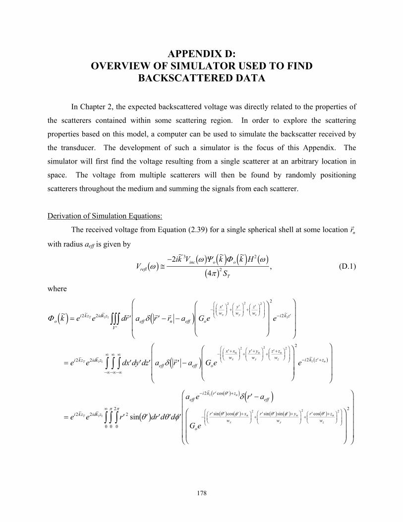
APPENDIX D: OVERVIEW OF SIMULATOR USED TO FIND
BACKSCATTERED DATA In Chapter 2, the expected backscattered voltage was directly related to the properties of
the scatterers contained within some scattering region. In order to explore the scattering
properties based on this model, a computer can be used to simulate the backscatter received by
the transducer. The development of such a simulator is the focus of this Appendix. The
simulator will first find the voltage resulting from a single scatterer at an arbitrary location in
space. The voltage from multiple scatterers will then be found by randomly positioning
scatterers throughout the medium and summing the signals from each scatterer.
Derivation of Simulation Equations:
The received voltage from Equation (2.39) for a single spherical shell at some location rn
with radius aeff is given by
Vik V k k H
Sreflinc o o
T
ωω ω
πb g b g d i d i b g
b g≅−2
4
3 2
2
~ ~ ~Ψ Φ, (D.1)
where
Φ oi kz idk z
eff n eff o
xw
yw
zw i k z
V
i kz idk zeff eff o
x xw
y y
k e e dr a r r a G e e
e e dx dy dz a r a G e
Tx y z
T
n
x
~ ~ ~ ~
~ ~
d i d i
d i
= ′ ′ − −
F
HGGG
I
KJJJ
F
H
GGG
I
K
JJJ
= ′ ′ ′ ′ −
−′FHGIKJ +
′FHGIKJ +
′FHGIKJ
FHGG
IKJJ
− ′
′
−′+FHG
IKJ +
′+
zzz2 2
2
2
2 2
1 1
2 2 2
1
1 1
2
δ
δn
y
n
zn
wz z
w i k z ze
FHG
IKJ +
′+FHGIKJ
FHGG
IKJJ − ′+
−∞
∞
−∞
∞
−∞
∞F
HGGG
I
KJJJ
F
H
GGG
I
K
JJJzzz2 2
1
2
2 ~ b g
= ′ ′ ′ ′ ′
′ −
F
HGGG
I
KJJJ
F
H
GGGGG
I
K
JJJJJ
− ′ ′ +
−′ ′ ′ +FHG
IKJ +
′ ′ ′ +FHG
IKJ +
′ ′ +FHG
IKJ
FHGG
IKJJ
∞ zzze e r dr d d
a e r a
G ei kz idk z
effi k r z
eff
o
r xw
r yw
r zw
T
n
n
x
n
y
n
z
2 2 2
2
2
0
2
00
1 1
1
2 2 2~ ~
~ cos
sin cos sin sin cossin θ θ φ
δθ
θ φ θ φ θππ
b gd ib gc h
b g b g b g b g b g
178
= ′ ′
′
F
HGGG
I
KJJJ
− ′ ′ +
−′ ′ +F
HGIKJ +
′ ′ +FHG
IKJ +
′ +FHG
IKJ
FHGG
IKJJ
z
z
a G e e e d
d e
eff oi k z idk z i k r z
a xw
a yw
a zw
T n
eff n
x
eff n
y
eff n
z
3 2 2 2 2
0
0
2 2
1 1 1
2 2 2
~ ~ ~ cos
sin cos sin sin cos
sin
.
θ θ
φ
θπ
πθ φ θ φ θ
b g b gc h
b g b g b g b g b g
(D.2)
Assuming that the source is circularly symmetric so that wx = wy, then Equation (D.2) becomes
Φ o eff oi kz idk z i k a z
a zw
wa x a
k a G e e e e d
d e
T eff n
eff n
z
xeff n eff n
~ sin~ ~ ~ cos
cos
sin cos sin sin
d i b g b gd ib g
b g b gd i b g b gd i
= ′ ′
′FHG
IKJ
− ′ +−
′ +
y
FHG
IKJ
−′ ′ + + ′ ′ +FH IK
zz
3 2 2 2 22
0
0
2 2
1 1 1
2
22 2
θ θ
φ
θθπ
π θ φ θ φ
= ′ ′
′FHG
IKJ
−+
− ′ +−
′ −′ +F
HGIKJ
−′ ′ + ′
zz
a G e e e e e e d
d e
eff ow
x yi kz idk z i k a z w
aa z
w
a
wx y
xn n
T eff n xeff
eff n
z
eff
xn n
3 22
2 2 22 2
0
0
2 4
22 2
1 1 1 22 2
2
2
e j b gd i b ge j b g
b g b g b gc h
b g~ ~ ~ cos sincos
sin cos sin
sin θ θ
φ
θ θθπ
π θ φ φ
= ′ ′
′F
HGG
I
KJJ
−+
− ′ +−
′ −′ +F
HGIKJ
− +′ ′ + ′
zz
a G e e e e e e d
d e
eff ow
x yi kz idk z i k a z w
aa z
w
a x y
w
xn n
T eff n xeff
eff n
z
eff n n
xn n
3 22
2 2 22 2
0
0
2 4
22 2
1 1 1 22 2
2
2 2
2
e j b gd i b ge j b g
b g b g b g b g b gc h
b g~ ~ ~ cos sincos
sin cos cos sin sin
sin θ θ
φ
θ θθπ
π θ φ φ φ φ
= ′ ′
′F
HGG
I
KJJ
=
−+
− ′ +−
′ −′ +F
HGIKJ
+′ ′−
−+
zz
a G e e e e e e d
d e
a G e e
eff ow
x yi kz idk z i k a z w
aa z
w
ii a x y
w
eff ow
x yi kz
xn n
T eff n xeff
eff n
z
eff n n
xn
xn n
T
3 22
2 2 22 2
0
0
2 4
3 22
2
22 2
1 1 1 22 2
2
2 2
2
22 2
e j b gd i b ge j b g
b g b g
e j
b g~ ~ ~ cos sincos
sin cos
~
sin θ θ
φ
θ θθπ
π θ φ φ
e e e e
Ji a x y
w
idk z i k a z wa
a zw
oeff n n
x
eff n xeff
eff n
z2 22 2
0
2 2
2
1 1 1 22 2
2
4
~ ~ cos sincos
sin
sin
′ ′
+′
FHGG
IKJJ
− ′ +−
′ −′ +F
HGIKJz θ θ
θ
θ θθπ
b g
b g
b gd i b ge j b gd
179
=′
+′
FHGG
IKJJ
F
H
GGGG
I
K
JJJJ′
− + −−
− ′−
′−
′ + ′
za G e e ee e e
Ji a x y
w
deff ow
x yz
w idk z i kz i k z
i k a wa
wa a z
oeff n n
x
xn n
n
z T n
eff xeff
zeff eff n
3 22 2
2 2 2
22 2
2
2 2
20
22 2
2
21 1 1
12
2 22
2 2
4e j
b g b g b g b ge jb g
b g~ ~ ~
~ cossin cos cos
sin
sin.
θ
θθ
θθ θ θ
π
(D.3)
Now perform the substitution of letting sθ θ= ′cosb g, so that Equation (D.3) becomes
Φ o eff ow
x y zw idk z i kz i k z
i k a s wa s
wa s a z s
oeff n n
x
eff ow
x y z
k a G e e ee e e
Ji a x y
ws
ds
a G e
xn n
n
z T n
eff xeff
zeff eff n
xn n
~ ~ ~ ~
~
d i e je j e j
e j
= +−
FHGG
IKJJ
F
H
GGGG
I
K
JJJJ
=
− + −−
−−
−−
+
−
− + −
z3 22 2
2 2 2
22 1 2 2
2 2
221
1
3 22 2
22 2
2
21 1 1
12
2 22
2 2
22 2
41
θθ θ θ
θ
θ
n
z T n
xeff
eff
z
eff zeff n
eff zeff n
w idk z i kz i k z
wa s
a s
wo
eff n n
x
i k a s wa z s
i k a s wa z s
e e
e e Ji a x y
ws
e e e e
ds2
21 1 1
22 2
2 2
2
12
12
2 2 2
2 12 2 2
22
24
24
0
1
41
~ ~ ~
~ ~
.−
−−
−
−−
+−
FHGG
IKJJ
+FHG
IKJ
F
H
GGGGGG
I
K
JJJJJJz
θθ
θθ
θθ
θ
θ
e j
(D.4)
In order to integrate Equation (D.4), assume that the scatterers are also small compared to the
width of the beam in the x, y, and z directions. In effect, this is the same as assuming the field is
constant across the surface of the scatterer. Then, to a first-order approximation, the integral
becomes
Φ o eff ow
x y zw idk z i kz i k z i k a s i k a s
eff ow
x y zw idk z i k z i k z
eff
eff ow
x y
k a G e e e e e ds
a G e e e k a s ds
a G e
xn n
n
z T n eff eff
xn n
n
z T n
xn n
~
cos ~
~ ~ ~ ~ ~
~ ~ ~
d i e j
d i
e j
e j
e
≅ +
≅
≅
− + −− −
− + −−
− +
zz
3 22 2
2 2 2 2 2
0
1
3 22 2
2 2 21
0
1
3 22
22 2
2
21 1 1 1 1
22 2
2
21 1 1
22 2
2 2
2
θ θθ
θ θ
j d i−−
22 2 2 1
1
2
21 1 1
2
2
zw idk z i k z i k z eff
eff
n
z T ne ek a
k a~ ~ ~ sin ~
~ ,
(D.5)
which is equivalent to the form factor for shells given by Insana et al. [1990].
Likewise, the scattering resulting from a single Gaussian scatterer can also be simulated.
In this case, the expression for Φo would be given by
180
Φ oidk z i kz
r rd
o
xw
yw
zw i k z
V
idk z i k zrd
o
x xw
y yw
k e e dr e G e e
e e dr e G e
T
nx y z
T
n
x
n
y
~ ~ ~
max
~
~ ~
max
d i = ′
F
HGGG
I
KJJJ
F
H
GGG
I
K
JJJ
= ′
−′− −
′FHGIKJ +
′FHGIKJ +
′FHGIKJ
FHGG
IKJJ
− ′
′
−′ −
′+FHG
IKJ +
′+FHG
IKJ
zzz2 2
2
2
2 2
1 1
2
2
2 2 2
1
1 1
2
2
2
γ
γ
2 2
1
2
2+
′+FHGIKJ
FHGG
IKJJ
− ′
′
F
HGGG
I
KJJJ
F
H
GGG
I
K
JJJzzzz z
w i k z
V
n
z e~
=
′ ′ ′ ′ ′
F
HGG
I
KJJ
F
H
GGGGG
I
K
JJJJJ
=
−′
− ′ ′ +
−′ ′ ′ +FHG
IKJ +
′ ′ ′ +FHG
IKJ +
′ ′ +FHG
IKJ
FHGG
IKJJ
∞ zzzγ
θ θ φ
γ
θ
θ φ θ φ θ
ππ
max
~ ~
~ cos
sin cos sin sin cos
max
sin
e e
r dr d d e e
G e
G
idk z i kz
rd i k r z
o
r xw
r yw
r zw
o
T
n
n
x
n
x
n
z
2 2
2 2
2
0
2
00
1 1
2
2 1
2 2 2
b g b gc h
b g b g b g b g b g
22
2 2 2
2
2 2
2
2 2 20
0
22 2
1 1 1
2
2
1
2 2
22
4e e e dr
r e
dJ
i r x yw
e
wx y
idk z i kz i k z
rd
on n
x
i k rr z
wrw
xn n
T n
n
z x
− +−
−′
− ′ ′ −′ ′ +FHG
IKJ −
′′
∞
′
′
′′
′ +′
FHG
IKJ
F
H
GGGG
I
K
JJJJ
F
H
GGGGGGG
I
K
JJJJJJJzz
e j
b g b g b g
b g b g~ ~ ~
~ coscos
sin
sin sinθ
θ θ
θθ
θ
π
= ′
′
′′
′ +′
FHG
IKJ
F
H
GGGG
I
K
JJJJ
F
H
GGGGGGG
I
− + −−
−′
− ′ ′ − ′ ′ + ′ ′ −′
′
zγ
θθ θ
θ θ θ
πmax
~ ~ ~
~ cos cos cos sin
sin sinG e e e dr
r e
dJ
i r x yw
e
ow
x yz
w idk z i kz i k z
rd
on n
x
i k rw
r r z rw
xn n
n
z T n
zn
x
22 2
2 2 2
2
2 2
2
2 2 2 20
22 2
2
21 1 1
2
2
1 22 2
2
22
4e j
b g b g b ge j b g
b g b g
θ
K
JJJJJJJ
≅ ′ ′′
′
FHGG
IKJJ
=FHG
IKJ ′ ′ ′
∞
− + −−
−′∞
− + −−
−
z
z
0
22 2
2 2 2 2 1
10
02
1
2 22 2 2
1
22 2
2
21 1 1
2
2
22 2
2
21 1 1
2
2
22
γ
γ
max
~ ~ ~
max ~ ~ ~
sin ~
~
~ sin ~
G e e e dr r ek r
k r
Gk
e e e dr r k r e
ow
x yz
w idk z i kz i k zrd
wx y
zw idk z i kz i k z
xn n
n
z T n
xn n
n
z T n
e j
e j
d i
d i′∞ F
HGIKJz r
d
2
2
0
,
(D.6)
where d is some characteristic length describing the Gaussian impedance distribution
(d ) [Insana et al., 1990]. The integral in Equation (D.6) can then be found by
integrating by parts to yield
aeff≅ 0 643.
181

dr r k r e d k r rd
e dr
d k r e k k r e dr
d kk r e dr
d ke
rd
rd
rd
rd
rd
k d
′ ′ ′FHG
IKJ= − ′ −
′′
FHG
IKJ
= − ′ + ′ ′FHGG
IKJJ
= − ′ ′FHG
IKJ
= −
−′∞ −
′∞
−′
∞−
′∞
−′∞
−
z z
z
z
sin ~ sin ~
sin ~ ~ cos ~
~cos ~
~~
22
2 2
22 2 2
22 2
2
10
2
1 20
2
1
0
1 10
21
10
31
2
2
2
2
2
2
2
2
2
2
12
d i d i
d i d i
d i
π 2
.
(D.7)
Hence, Equation (D.6) becomes
Φ ow
x y zw idk z i kz i k z k d
effw
x y zw idk z i kz i k z k a
k Gk
e e e d k e
a G e e e e
xn n
n
z T n
xn n
n
z T n eff
~~
~
.
max~ ~ ~ ~
max
~ ~ ~ . ~
d i
b g
e j
e j
= −FHG
IKJ
= −
− + −− −
− + −− −
γ π
γ
02
1
2 22 2 2
31
302
2 22 2 2 0 4136
2 2
01178
22 2
2
21 1 1 1
2 2
22 2
2
21 1 1 1
2 2
(D.8)
which is also equivalent to the form factor for Gaussian spheres given by Insana et al. [1990].
Now that an expression for the scattering from a single scatterer has been obtained, either
shell or Gaussian, scattering from multiple randomly oriented scatterers of various sizes can be
found by simply adding up the contribution from each of the scatterers. Hence, for n scatterers
per unit volume, the total scattered field at any given frequency would be given by
Vik V k H
Sk a x y zrefl
inc o
To eff n n
n
N
ωω ω
πb g b g d i b g
b g d≅−
=∑
2
4
3 2
21
n i~ ~
~; , , ,Ψ
Φ , (D.9)
where
N n w w
x w wy w w
z
xo yo
n xo xo x
n yo yo y
n z
= ⋅
= − += − +
= − +
10 10 16
5 105 10
8 16
b gd ib g
b g
mm
mm mm
χχ
χ
(D.10)
after limiting the scatterers to a reasonable number near the focus with wxo,yo being the Gaussian
beamwidths at the center frequency for the transducer. χx,y,z are random variables satisfying a
uniform distribution with possible values ranging from zero to one. Scatterers were only
positioned to within 8 mm of the focus along the beam axis to improve computation time, and
182
the simulation studies were always restricted to this region. However, for some of the
simulations, Equation (D.10) was modified as
N n w w
x w wy w w
z
xo yo
n xo xo x
n yo yo y
n z
= ⋅
= − += − +
= − +
30 30 16
15 3015 30
8 16
b gd ib g
b g
mm
mm mm
χχ
χ
(D.11)
in order to include scatterers in a larger region about the focus.
Before concluding, the generation of the simulated waveforms is based on several
approximations rather than a complete physics-capturing model in order to reduce the
computational complexity (i.e., ~ 20 as compared to ~ 1x10⁶ operations per scatterer at each
frequency assuming λ/20 gird spacing for a scatterer of radius λ/4 and order N 2 on the matrix
inversion for the complete solution). These approximations should be justified. First, the
simulator neglects multiple scattering, however, this approximation was shown to be valid by
comparing the experimental phantom results to the simulation results in Chapter 3. Second, the
simulator approximates the real velocity field from the focused source as a three-dimensional
Gaussian distribution rather than solving for the complete field exactly. Once again, the
validation of this approximation is demonstrated in Appendix E. Third, the generated
waveforms do not consider the generation of shear waves (i.e., mode conversions) at the surface
of the scatterer.
Shear waves are not significant in soft biological tissue at a macroscopic scale [Haken et
al., 1992]. However, shear waves may modify the scattering from individual scatterers at which
point the simplified simulator presented in this Appendix would need to be modified. Namely,
the calculation of the scattering from a single scatterer Φo would need to be modified to include
shear waves. For simple scatterers, an expression for the scattering could still be solved in
closed form, but the more complicated scatterers would require a numerical method (i.e., finite
element or possibly method of moments) to find the scattering. Multiple scattering, however,
would still not need to be included.
Matlab Code Used to Generate Received Voltage for Gaussian Scatterers: clear all; close all;
183
i=sqrt(-1); %%%%%%%%%%%%%%%%%%%%%%%%%%%%%%%%%%%%%%%%%%%%%%%%%%%%%%%% %BACKSCATTER SIMULATION % %%%%%%%%%%%%%%%%%%%%%%%%%%%%%%%%%%%%%%%%%%%%%%%%%%%%%%%% %This is a program that computes the acoustic signal % %scattered from a tissue region buried beneath N-layers% %of distinct tissue types. The simulation neglects % %multiple scattering and assumes that the Born % %approximation is valid. Region 1 is the layer with % %scatterers, and Region N is the layer with the % %transducer. The simulation assumes that the scatterers% %are Gaussian distributions. % %%%%%%%%%%%%%%%%%%%%%%%%%%%%%%%%%%%%%%%%%%%%%%%%%%%%%%%% %%%%%%%%%%%%%%%%%%%%%%%%%%%%%%%%%%%%%%%%%%%%%%%%%%%%%%%% %Enter properties of the different layers. % %%%%%%%%%%%%%%%%%%%%%%%%%%%%%%%%%%%%%%%%%%%%%%%%%%%%%%%% %Enter the number of layers and density of scatterers N=1; nbar=5*(1000)^3; %#/m^3 nbar_mult=7; mbar=nbar*nbar_mult; %Enter the density and sound speed for each layer. %******************************************************% %Typical Values for Different Tissue Types % %******************************************************% %Tissue Density(Kg/m^3) Speed(m/s)_2 % % Fat 850_1,937_3 1476-1487 % % Muscle 1050_1,1070_3 1500-1610 % % Liver 1050_1,1064_3 1532-1570 % % Brain 1021-1079_2 1501-1568 % % Skull 1738-1914_2 2010-3360 % % Bone (Cortical) 1700_1 3176-3406 % % % %1. Data from Table 4.1, pg. 53, NCRP Report No. 113. % %2. Human data Goss, Johnston, and Dunn "Ultrasonic % % properties of mammalian tissues," JASA, 1978. % %3. Pig data Goss, Johnston, and Dunn "Ultrasonic % % properties of mammalian tissues," JASA, 1978. % %******************************************************% rho_liver=1050;%+14*rand(1); rho_muscle=1050;%+20*rand(1); rho_fat=850;%+87*rand(1); rho_water=1000; rho=[rho_liver rho_muscle rho_fat rho_water]; c_liver=1532;%+38*rand(1); c_muscle=1500;%+110*rand(1); c_fat=1476;%+11*rand(1); c_water=1540;
184

c=[c_liver c_muscle c_fat c_water]; %Find Transmission coefficients T=1; for ti=1:(N-1) Tij=2*rho(ti+1)*c(ti+1)/(rho(ti+1)*c(ti+1) + rho(ti)*c(ti)); Tji=2*rho(ti)*c(ti)/(rho(ti+1)*c(ti+1) + rho(ti)*c(ti)); T=T*Tij*Tji; end %Enter the attenuation properties for each layer. %******************************************************% %Typical Values for Different Tissue Types % %******************************************************% %Tissue Attenuation a*f^b % % alpha_0(Np/cm/MHz^-b) b % % Fat 0.053_5 1_5 % % Muscle % % Perpendicular 0.0145_3 1.90_3 % % 0.13-0.18_4 1_4 % % Parallel 0.3626_3 1.20_3 % % 0.33-0.47_4 1_4 % % Liver 0.032-0.034_1 1.30-1.32_1 % % 0.08_2 1.13_2 % % Brain 0.07_2 1.14_2 % % White 0.064_1 1.27_1 % % Grey 0.012_1 1.17_1 % % Bone (Cortical) 0.46_4 1_4 % % % %1. Lyons and Parker "Absorption and attenuation in % % soft tissues II - experimental results," IEEE, 1988% %2. Goss, Frizzell, and Dunn "Ultrasonic absorption % % and attenuation in mammalian tissues," UMB, 1979. % %3. Kudo et al. "Basic study on the ultrasound % % attenuation of fibrous biological tissue in the % % frequency range of 10-40 MHz," IEEE-US, 1998. % %4. Goss, Johnston, and Dunn "Compilation of empirical % % properties of mammalian tissues. II," JASA, 1980. % %5. Data from Table 5.2, pg. 64, NCRP Report No. 113. % %******************************************************% alpha_0=input('Enter attenuation in Np/cm/MHz:'); b=1; %Give z location of each layer boundary. z=[5e-2 2.6e-2 3e-2]; %m %%%%%%%%%%%%%%%%%%%%%%%%%%%%%%%%%%%%%%%%%%%%%%%%%%%%%%%% %Enter properties of the transducer. % %%%%%%%%%%%%%%%%%%%%%%%%%%%%%%%%%%%%%%%%%%%%%%%%%%%%%%%% %******************************************************% F=5e-2; %m focal length f_num=4; %f# of transducer fo=8e6; %Circuit resonance frequency for the transducer.
185
rel_zo=0; %Distance from focus to plate as fraction of zT. %******************************************************% a_source=0.5*F/f_num; %Transducer aperture radius zT=sqrt(F^2 - a_source^2); %Distance to aperture plane. zo=zT*rel_zo; St=pi*a_source^2; %Focal gain of transducer. Go=a_source^2/(2*F); wx_m=0.87*f_num; wz_m=6.01*(f_num^2); lambda_o=c(1)/fo; wx_o=wx_m*lambda_o; wz_o=wz_m*lambda_o; %%%%%%%%%%%%%%%%%%%%%%%%%%%%%%%%%%%%%%%%%%%%%%%%%%%%%%%% %Determin Acoustic pulse in aperture plane % %%%%%%%%%%%%%%%%%%%%%%%%%%%%%%%%%%%%%%%%%%%%%%%%%%%%%%%% %Assume Kuv=1 %******************************************************% BW=2e6 %Width of Gaussian describing transducer filtering. vp=1000; %Amplitude of voltage spike excitation. Kuv=1;%m/s V^-1 %******************************************************% %Set incident voltage for each frequency. dt=0.15/fo; %Sampling time separation. Tp=2*(F+20e-3)/c(1); %Length of time window of interest. v=zeros(1,ceil(Tp/dt)); %Excitation pulse. v(35)=vp; %time1=35, time2=35 if mod(length(v),2) v=[v 0]; end time=dt*[0:length(v)-1]; offset=time(35); %time1=35, time2=35 %Determine value for each frequency Vinc=(ifft(v)); M=length(Vinc); Vinc_p=Vinc(1:M/2); %Find corresponding freq. values d_f1=[0:(M/2-1)]*2*pi/M; d_f2=[(M/2):(M-1)]*2*pi/M - 2*pi;
186

%freq=[d_f1 d_f2]*(1/dt)/(2*pi); freq=[d_f1]*(1/dt)/(2*pi); %Set Filtering Characteristics of Source. H=abs(freq).*exp(-((abs(freq)-fo)/BW).^2); %Use Rayleigh Distribution H=H/max(H); Uz_o=Kuv*Vinc_p.*H; uz_o=real(fft(Uz_o,M)); figure(1) clf plot(time*1e6,uz_o) xlabel('Time (\mus)') ylabel('Particle Velocity at Center of Aperture (m/s)') grid figure(2) clf plot(freq*1e-6,abs(Uz_o)/max(abs(Uz_o))) xlabel('Frequency (MHz)') ylabel('Normalized |U_z(0,0,z_T,\omega)|') grid axis([min(freq*1e-6) max(freq*1e-6) 0 1]) %%%%%%%%%%%%%%%%%%%%%%%%%%%%%%%%%%%%%%%%%%%%%%%%%%%%%%%% %Enable to run many simulations in a row % %%%%%%%%%%%%%%%%%%%%%%%%%%%%%%%%%%%%%%%%%%%%%%%%%%%%%%%% sv = input('Save data: y/n ','s'); path='/u1_peur/bigelow/Backscatter_Simulation/simulation_data/'; if sv=='y' n=input('Enter filename to save scattered voltage and time: ','s'); Num_Files=input('Enter number of independent scatterer ... distributions: '); else Num_Files = 1; end aeff_enter=input('Enter size of scatterers in micrometers: '); aeff_enter=aeff_enter*1e-6; clear uz_o figure(77) clf hold grid time_start=clock; for file_index=1:Num_Files
187
figure(77) plot(etime(clock,time_start),100*(file_index-1)/Num_Files,'x') V_scat=zeros(size(freq)); for mi=1:nbar_mult %%%%%%%%%%%%%%%%%%%%%%%%%%%%%%%%%%%%%%%%%%%%%%%%%%%%%%%% %Find Scattered Field at each Frequency % %%%%%%%%%%%%%%%%%%%%%%%%%%%%%%%%%%%%%%%%%%%%%%%%%%%%%%%% %Determine number of scatterers Numscat=ceil(nbar*100*wx_o*wx_o*(16e-3)) aeff=aeff_enter g_max=1; Vs=zeros(1,length(freq)); xn=-5*wx_o + 10*wx_o*rand(1,Numscat); yn=-5*wx_o + 10*wx_o*rand(1,Numscat); zn=-8e-3 + 16e-3*rand(1,Numscat); ko=2*pi*freq/c_water; k=2*pi*freq/c(1); alpha=100*alpha_0(1)*(freq/1e6).^b(1); k_comp=k+i*alpha; lambda=c(1)./freq; wx=wx_m*lambda; wz=wz_m*lambda; Psi=-2*i*((k_comp/(4*pi)).^2)*T; %Find V_scat term1=-0.1178 * g_max * Go^2 * aeff^3; term2a=exp(i*2*k_comp*zT); %Vector in Freq. term2b=exp(-i*2*k_comp'*zn); %Matrix in frequency, scatterer % number term3=exp(-2*(((wx.^-1)'*xn).^2 + ((wx.^-1)'*yn).^2 + ... ((wz.^-1)'*zn).^2)); %Matrix in frequency, scatterer number term4=exp(-0.4136*k_comp.^2*aeff^2); %Vector in frequency. term_freq_vector=(term1.*term2a.*term4 ... .*Psi.*k_comp.*Vinc_p.*H.*H/St); term_freq_vector2=((term2b.*term3)*ones(Numscat,1))'; Vs=(term_freq_vector.*term_freq_vector2).*(freq>1);
188

V_scat=V_scat+Vs; end %Find V_plate termA=-(ko.^2.*wx.^2)*(Go^2) .* Vinc_p .* H .* H/(St*8*pi); termB=exp(i*ko*(2*zT - 2*zo)); termC=exp(-(zo./wz).^2); V_plate=(termA.*termB.*termC).*(freq>1); figure(3) clf plot(freq*1e-6,abs(V_scat)/max(abs(V_scat))) grid hold plot(freq*1e-6,abs(V_plate)/max(abs(V_plate)),'r-.') xlabel('Frequency (MHz)') ylabel('Normalized |V|') %%%%%%%%%%%%%%%%%%%%%%%%%%%%%%%%%%%%%%%%%%%%%%%%%%%%%%%% %Find Scattered Field in Time Domain % %%%%%%%%%%%%%%%%%%%%%%%%%%%%%%%%%%%%%%%%%%%%%%%%%%%%%%%% v_scat=real(fft(V_scat,M)); figure(4) clf plot(time*1e6,v_scat) xlabel('Time (\mus)') ylabel('Scattered Voltage (V)') grid %%%%%%%%%%%%%%%%%%%%%%%%%%%%%%%%%%%%%%%%%%%%%%%%%%%%%%%% %PLATE SCATTER SIMULATION % %%%%%%%%%%%%%%%%%%%%%%%%%%%%%%%%%%%%%%%%%%%%%%%%%%%%%%%% V_plate(1) = 0; v_plate=real(fft(V_plate,M)); figure(5) clf plot(time*1e6,v_plate) xlabel('Time (\mus)') ylabel('Plane Voltage (V)') grid TIME=time'; VSCAT_TIME(:,file_index)=v_scat'; end %%%%%%%%%%%%%%%%%%%%%%%%%%%%%%%%%%%%%%%%%%%%%%%%%%%%%%%% %Save Scattered Field to File %
189
%%%%%%%%%%%%%%%%%%%%%%%%%%%%%%%%%%%%%%%%%%%%%%%%%%%%%%%% if sv=='y' txtfile=[path n '.txt']; fid=fopen(txtfile,'w'); for ti=1:length(time) fprintf(fid,'%2.6e ',time(ti)); for fi=1:(Num_Files-1) fprintf(fid,' %2.6e ',VSCAT_TIME(ti,fi)); end fprintf(fid,' %2.6e \n',VSCAT_TIME(ti,Num_Files)); end fclose(fid); end sv = input('Save Plate voltage and time: y/n ','s'); if sv=='y' n=input('Enter filename to save Plate voltage and time: ','s'); name=[path n]; txtfile=[path n '.txt']; fid=fopen(txtfile,'w'); for ti=1:length(time) fprintf(fid,'%2.6e ',time(ti)); fprintf(fid,'%2.6e \n',v_plate(ti)); end fclose(fid); end sv = input('Save parameters: y/n ','s'); if sv=='y' n=input('Enter filename to save parameters: ','s'); txtfile=[path n '.txt']; fid=fopen(txtfile,'w'); fprintf(fid,'c (m/s) = %f \n',c(1)); fprintf(fid,'aeff (um) = %f \n',aeff*1e6); fprintf(fid,'alpha (Np/cm MHz^-b) = %f \n',alpha_0); fprintf(fid,'b = %f \n',b); fprintf(fid,'F (cm) = %f \n',F*100); fprintf(fid,'f_num = %f \n',f_num); fprintf(fid,'fo (MHz) = %f \n',fo*1e-6); fprintf(fid,'BW (MHz) = %f \n',BW*1e-6); fprintf(fid,'nbar (#/mm^3) = %f \n',mbar/1e9);
190
fprintf(fid,'wx_m = %f \n',wx_m); fprintf(fid,'wy_m = %f \n',wx_m); fprintf(fid,'wz_m = %f \n',wz_m); fprintf(fid,'zT (cm) = %f \n',zT*100); fprintf(fid,'dt*fo = %f \n',dt*fo); fprintf(fid,'offset (us) = %f \n',offset*1e6); fclose(fid); end
Matlab Code Used to Generate Received Voltage for Shell Scatterers:
clear all; close all; i=sqrt(-1); %%%%%%%%%%%%%%%%%%%%%%%%%%%%%%%%%%%%%%%%%%%%%%%%%%%%%%%% %BACKSCATTER SIMULATION % %%%%%%%%%%%%%%%%%%%%%%%%%%%%%%%%%%%%%%%%%%%%%%%%%%%%%%%% %This is a program that computes the acoustic signal % %scattered from a phantom. The simulation neglects % %multiple scattering and assumes that the Born % %approximation is valid. Region 1 is the phantom, and % %Region 2 is the water containing the transducer. % %The simulation assumes that the scatterers are shells.% %%%%%%%%%%%%%%%%%%%%%%%%%%%%%%%%%%%%%%%%%%%%%%%%%%%%%%%% %%%%%%%%%%%%%%%%%%%%%%%%%%%%%%%%%%%%%%%%%%%%%%%%%%%%%%%% %Enter properties of the different layers. % %%%%%%%%%%%%%%%%%%%%%%%%%%%%%%%%%%%%%%%%%%%%%%%%%%%%%%%% %Enter the number of layers and density of scatterers N=2; %Enter the density and sound speed for each layer. rho_phantom=1040; rho_water=1000; rho=[rho_phantom rho_water]; Temp=input('Enter temperature to calculate sound speed:'); Phan_Num=input('Enter Phantom Number (1=A, 2=B):'); c_water=CfromT(Temp); if Phan_Num==1 alpha0=6.3597/100; %Np/cm/MHz c_phantom=1534.4; %m/s nbar=5.1135*(1000)^3; %20.454#/m^3 nbar_mult=4; mbar=nbar*nbar_mult;
191
else alpha0=9.5140/100; %Np/cm/MHz c_phantom=1539.6; %m/s nbar=5.9658*(1000)^3; %47.7266#/m^3 nbar_mult=8; mbar=nbar*nbar_mult; end b=1; c_phantom=c_phantom - 1.7*(22-Temp); c=[c_phantom c_water]; %Find Transmission coefficients T=1; for ti=1:(N-1) Tij=2*rho(ti+1)*c(ti+1)/(rho(ti+1)*c(ti+1) + rho(ti)*c(ti)); Tji=2*rho(ti)*c(ti)/(rho(ti+1)*c(ti+1) + rho(ti)*c(ti)); T=T*Tij*Tji; end %Now consider window. ff=[7 8 9]; TT=[.7910 .7491 .7093]; TTwin=polyfit(ff,TT,1); %Give z location of each layer boundary. Fdis=input('Enter distance to aperture plane of the transducer in m:'); zT=input('Enter distance from focal plane to surface of phantom in m:'); %z=[Fdis zT]; %m %%%%%%%%%%%%%%%%%%%%%%%%%%%%%%%%%%%%%%%%%%%%%%%%%%%%%%%% %Enter properties of the transducer. % %%%%%%%%%%%%%%%%%%%%%%%%%%%%%%%%%%%%%%%%%%%%%%%%%%%%%%%% f_num=input('Enter f-number for the transducer:'); a_source=input('Enter radius of transducer aperture in m:'); St=pi*a_source^2; F=sqrt(Fdis^2 + a_source^2); %Focal length of transducer. %Focal gain of transducer. Go=a_source^2/(2*F); wx_m=0.87*f_num; wz_m=input('Enter slope of wz (wz_m):'); wz_o=input('Enter intercept of wz (wz_o) in m:'); lambda_o=c(1)/9e6;
192
wx0=wx_m*lambda_o; wz0=wz_m*lambda_o+wz_o; %%%%%%%%%%%%%%%%%%%%%%%%%%%%%%%%%%%%%%%%%%%%%%%%%%%%%%%% %Determine Acoustic pulse in aperture plane % %%%%%%%%%%%%%%%%%%%%%%%%%%%%%%%%%%%%%%%%%%%%%%%%%%%%%%%% %******************************************************% fo=input('Enter value for fo in MHz:'); fo=fo*1e6; %Rayleigh resonance frequency for the transducer. BW=input('Enter value for BW in MHz:'); BW=BW*1e6; %Width of Rayleigh describing transducer filtering. vp=1000; %Amplitude of voltage spike excitation. Kuv=1;%m/s V^-1 %******************************************************% %Set incident voltage for each frequency. dt=1/1e8; %Sampling time separation. Tp=2*(F+20e-3)/c(1); v=zeros(1,ceil(Tp/dt)); %Excitation pulse. v(50)=vp; %f/4=35, f/2,1=50 %%%%%%%%%%%%%%%%%%%%%%%%%%%%%%%%%%%%%%%%%%%%%%%%%%%%%%% if mod(length(v),2) v=[v 0]; end time=dt*[0:length(v)-1]; offset=time(50); %f/4=35, f/2,1=50 %%%%%%%%%%%%%%%%%%%%%%%%%%%%%%%%%%%%%%%%%%%%%%%% %Determine value for each frequency Vinc=(ifft(v)); M=length(Vinc); Vinc_p=Vinc(1:M/2); %Find corresponding freq. values d_f1=[0:(M/2-1)]*2*pi/M; d_f2=[(M/2):(M-1)]*2*pi/M - 2*pi; freq=[d_f1]*(1/dt)/(2*pi); %Set Filtering Characteristics of Source. H=abs(freq).*exp(-((abs(freq)-fo)/BW).^2); %Use Rayleigh Distribution H=H/max(H); Uz_o=Kuv*Vinc_p.*H; uz_o=real(fft(Uz_o,M));
193
figure(1) clf plot(time*1e6,uz_o) xlabel('Time (\mus)') ylabel('Particle Velocity at Center of Aperture (m/s)') grid figure(2) clf plot(freq*1e-6,abs(Uz_o)/max(abs(Uz_o))) xlabel('Frequency (MHz)') ylabel('Normalized |U_z(0,0,z_T,\omega)|') grid axis([min(freq*1e-6) max(freq*1e-6) 0 1]) %%%%%%%%%%%%%%%%%%%%%%%%%%%%%%%%%%%%%%%%%%%%%%%%%%%%%%%% %Enable to run many simulations in a row % %%%%%%%%%%%%%%%%%%%%%%%%%%%%%%%%%%%%%%%%%%%%%%%%%%%%%%%% sv = input('Save data: y/n ','s'); path='/u1_peur/bigelow/Backscatter_Simulation/simulation_data/'; if sv=='y' n=input('Enter filename to save scattered voltage and time: ','s'); Num_Files=input('Enter number of independent scatterer distributions: '); else Num_Files = 1; end clear uz_o for file_index=1:Num_Files V_scat=zeros(size(freq)); for mi=1:nbar_mult %%%%%%%%%%%%%%%%%%%%%%%%%%%%%%%%%%%%%%%%%%%%%%%%%%%%%%%% %Find Scattered Field at each Frequency % %%%%%%%%%%%%%%%%%%%%%%%%%%%%%%%%%%%%%%%%%%%%%%%%%%%%%%%% %Determine number of scatterers Numscat=ceil(nbar*100*wx0*wx0*(16e-3)) aeff=24.5e-6; g_max=1; Vs=zeros(1,length(freq)); xn=-5*wx0 + 10*wx0*rand(1,Numscat); yn=-5*wx0 + 10*wx0*rand(1,Numscat); zn=-8e-3 + 16e-3*rand(1,Numscat); ko=2*pi*freq/c_water; k=2*pi*freq/c(1); alpha=100*alpha0*(freq/1e6).^b;
194

k_comp=k+i*alpha; lambda=c(1)./freq; wx=wx_m*lambda; wz=wz_m*lambda + wz_o; TTFix=polyval(TTwin,freq*1e-6); Psi=-2*i*((k_comp/(4*pi)).^2)*T.*TTFix; %Find V_scat term1=2 * Go^2 * aeff^3; term2a=exp(i*2*k_comp*zT+i*2*ko*(Fdis-zT)); %Vector in Freq. term2b=exp(-i*2*k_comp'*zn); %Matrix in frequency, scatterer %number term3=exp(-2*(((wx.^-1)'*xn).^2 + ((wx.^-1)'*yn).^2 + ... ((wz.^-1)'*zn).^2)); %Matrix in frequency, scatterer number term4=sinc(2*k_comp*aeff/pi); %Vector in frequency. term_freq_vector=(term1.*term2a.*term4 ... .*Psi.*k_comp.*Vinc_p.*H.*H/St); term_freq_vector2=((term2b.*term3)*ones(Numscat,1))'; Vs=(term_freq_vector.*term_freq_vector2).*(freq>1); V_scat=V_scat+Vs; end %Find V_plate termA=-(ko.^2.*wx.^2)*(Go^2) .* Vinc_p .* H .* H/(St*8*pi); termB=exp(i*ko*(2*Fdis)); V_plate=(termA.*termB).*(freq>1); figure(3) clf plot(freq*1e-6,abs(V_scat)/max(abs(V_scat))) grid hold plot(freq*1e-6,abs(V_plate)/max(abs(V_plate)),'r-.') xlabel('Frequency (MHz)') ylabel('Normalized |V|') %%%%%%%%%%%%%%%%%%%%%%%%%%%%%%%%%%%%%%%%%%%%%%%%%%%%%%%% %Find Scattered Field in Time Domain % %%%%%%%%%%%%%%%%%%%%%%%%%%%%%%%%%%%%%%%%%%%%%%%%%%%%%%%%
195
v_scat=real(fft(V_scat,M)); figure(4) clf plot(time*1e6,v_scat) xlabel('Time (\mus)') ylabel('Scattered Voltage (V)') grid %%%%%%%%%%%%%%%%%%%%%%%%%%%%%%%%%%%%%%%%%%%%%%%%%%%%%%%% %PLATE SCATTER SIMULATION % %%%%%%%%%%%%%%%%%%%%%%%%%%%%%%%%%%%%%%%%%%%%%%%%%%%%%%%% V_plate(1) = 0; v_plate=real(fft(V_plate,M)); figure(5) clf plot(time*1e6,v_plate) xlabel('Time (\mus)') ylabel('Plane Voltage (V)') grid TIME=time'; VSCAT_TIME(:,file_index)=v_scat'; end %%%%%%%%%%%%%%%%%%%%%%%%%%%%%%%%%%%%%%%%%%%%%%%%%%%%%%%% %Save Scattered Field to File % %%%%%%%%%%%%%%%%%%%%%%%%%%%%%%%%%%%%%%%%%%%%%%%%%%%%%%%% if sv=='y' txtfile=[path n '.txt']; fid=fopen(txtfile,'w'); for ti=1:length(time) fprintf(fid,'%2.6e ',time(ti)); for fi=1:(Num_Files-1) fprintf(fid,' %2.6e ',VSCAT_TIME(ti,fi)); end fprintf(fid,' %2.6e \n',VSCAT_TIME(ti,Num_Files)); end fclose(fid); end sv = input('Save Plate voltage and time: y/n ','s'); if sv=='y'
196

197
n=input('Enter filename to save Plate voltage and time: ','s'); name=[path n]; txtfile=[path n '.txt']; fid=fopen(txtfile,'w'); for ti=1:length(time) fprintf(fid,'%2.6e ',time(ti)); fprintf(fid,'%2.6e \n',v_plate(ti)); end fclose(fid); end sv = input('Save parameters: y/n ','s'); if sv=='y' n=input('Enter filename to save parameters: ','s'); txtfile=[path n '.txt']; fid=fopen(txtfile,'w'); fprintf(fid,'c_phantom (m/s) = %f \n',c_phantom); fprintf(fid,'c_water (m/s) = %f \n',c_water); fprintf(fid,'alpha (Np/cm MHz^-b) = %f \n',alpha0); fprintf(fid,'b = %f \n',b); fprintf(fid,'Phan_Num = %f \n', Phan_Num); fprintf(fid,'Temp = %f \n', Temp); fprintf(fid,'F (cm) = %f \n',F*100); fprintf(fid,'Fdis (cm) = %f \n',Fdis*100); fprintf(fid,'zT (cm) = %f \n',zT*100); fprintf(fid,'f_num = %f \n',f_num); fprintf(fid,'a_source (cm) = %f \n',a_source*100); fprintf(fid,'wx_m = %f \n',wx_m); fprintf(fid,'wy_m = %f \n',wx_m); fprintf(fid,'wz_m = %f \n',wz_m); fprintf(fid,'wz_o = %f \n',wz_o); fprintf(fid,'fo (MHz) = %f \n',fo*1e-6); fprintf(fid,'BW (MHz) = %f \n',BW*1e-6); fprintf(fid,'nbar (#/mm^3) = %f \n',mbar/1e9); fprintf(fid,'dt = %f \n',dt); fprintf(fid,'offset (us) = %f \n',offset*1e6); fclose(fid); end
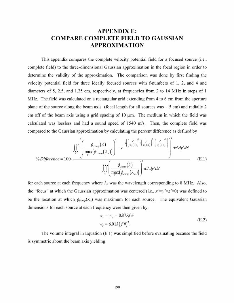
APPENDIX E: COMPARE COMPLETE FIELD TO GAUSSIAN
APPROXIMATION
This appendix compares the complete velocity potential field for a focused source (i.e.,
complete field) to the three-dimensional Gaussian approximation in the focal region in order to
determine the validity of the approximation. The comparison was done by first finding the
velocity potential field for three ideally focused sources with f-numbers of 1, 2, and 4 and
diameters of 5, 2.5, and 1.25 cm, respectively, at frequencies from 2 to 14 MHz in steps of 1
MHz. The field was calculated on a rectangular grid extending from 4 to 6 cm from the aperture
plane of the source along the beam axis (focal length for all sources was ~ 5 cm) and radially 2
cm off of the beam axis using a grid spacing of 10 µm. The medium in which the field was
calculated was lossless and had a sound speed of 1540 m/s. Then, the complete field was
compared to the Gaussian approximation by calculating the percent difference as defined by
%max
max
Difference
e d
dx dy dz
comp
V comp o
xw
yw
zw
V
comp
V comp oV
x y z
= ⋅
FHGG
IKJJ − x dy dz
F
HGGG
I
KJJJ
′ ′ ′
FHGG
IKJJ ′ ′ ′
′
−′F
HGIKJ +
′FHG
IKJ +
′FHG
IKJ
FHGG
IKJJ
′
′′
zzz
zzz100
22
2
4
2 2 2
φ λφ λ
φ λφ λ
λ λ λb gb gd i
b gb gd i
b g b g b g
(E.1)
for each source at each frequency where λo was the wavelength corresponding to 8 MHz. Also,
the “focus” at which the Gaussian approximation was centered (i.e., x’=y’=z’=0) was defined to
be the location at which φcomp(λo) was maximum for each source. The equivalent Gaussian
dimensions for each source at each frequency were then given by,
w w f
w fx y
z
= =
=
087
6 01 2
. #
. # .
λ
λb g (E.2)
The volume integral in Equation (E.1) was simplified before evaluating because the field
is symmetric about the beam axis yielding
198

%max
max
Difference
e r dr dz
r dr dz
comp
V comp o
rw
zw
r
L
L
comp
V comp o
r
L
L
x zmax
max
= ⋅
FHGG
IKJJ −
F
HGGG
I
KJJJ
′ ′ ′
FHGG
IKJJ ′ ′ ′
′
−′F
HGIKJ +
′FHG
IKJ
FHGG
IKJJ
−
′−
zz
zz100
22
2
02
2
4
02
2
2 2
φ λφ λ
φ λφ λ
ρ
λ λ
ρ ρ
ρ ρ
b gb gd i
b gb gd i
b g b g
(E.3)
where the limits of integration were set by using a window length of L = 13 mm and
r fmax = ⋅12 5 051. . #λb g and ′ = ′ + ′yρ2r x . The double integral in Equation (E.3) was then
evaluated using double integration function in Matlab based on the adaptive-recursive Newton-
Cotes 8 panel rule where φ
2
comp values away from the grid points were linearly extrapolated from
the closest grid values. In addition to calculating the percent difference according to Equation
(E.3), the percent difference was also calculated from
%max
max
Difference
e d
dz
comp
V comp o
zw
L
L
comp
V comp oL
L
z
= ⋅
zFHGG
IKJJ −
F
HGG
I
KJJ ′
FHGG
IKJJ ′
′
−′F
HGIKJ
−
′−
z
z100
22
2
2
2
4
2
2
2
φ λφ λ
φ λφ λ
λb gb gd ib gb gd i
b g
(E.4)
also using an L of 13 mm due to the importance of Gaussian approximation of the field along the
beam axis in the equation for the generalized attenuation-compensation function presented in
Chapter 2.
The percent differences from Equations (E.3) and (E.4) for all three sources at each
frequency are given in Figure E.1. The percent difference calculated over the entire field is
always less than 18.75%, indicating that assuming the velocity potential field is a three-
dimensional Gaussian distribution is a reasonable approximation. However, before concluding,
the differences between the complete and Gaussian fields were explored in greater detail. The
percent differences calculated from Equations (E.3) and (E.4) both exhibit a large increase after a
frequency of 8 MHz for the f/4 transducer. However, the percent differences from both
equations for the f/1 transducer are relatively constant with frequency with the results from
Equation (E.3) plateauing at ~18%. Likewise, the percent differences for the f/2 transducer as
given by Equation (E.3) also seem to approach a plateau of ~18% while the percent differences
from Equation (E.4) are relatively constant with frequency. Hence, the percent differences for
199
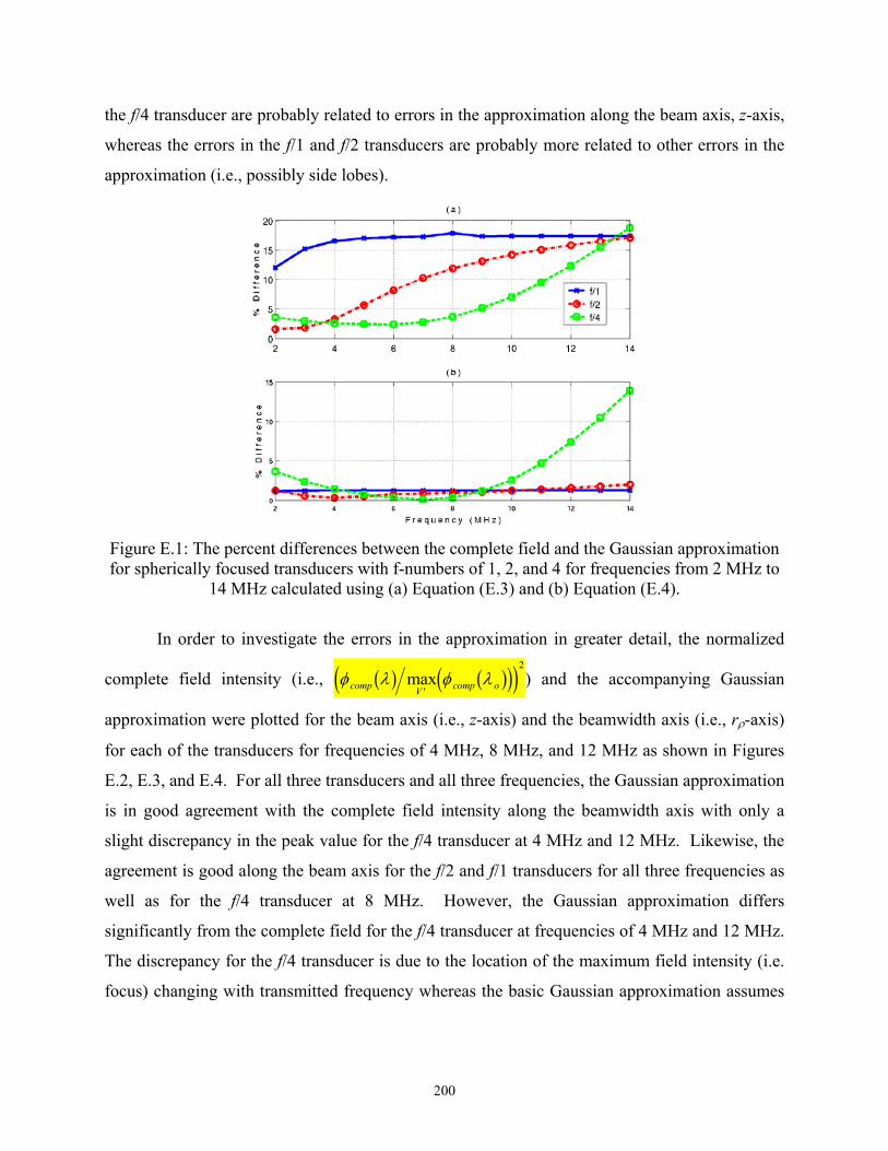
the f/4 transducer are probably related to errors in the approximation along the beam axis, z-axis,
whereas the errors in the f/1 and f/2 transducers are probably more related to other errors in the
approximation (i.e., possibly side lobes).
Figure E.1: The percent differences between the complete field and the Gaussian approximation for spherically focused transducers with f-numbers of 1, 2, and 4 for frequencies from 2 MHz to
14 MHz calculated using (a) Equation (E.3) and (b) Equation (E.4).
In order to investigate the errors in the approximation in greater detail, the normalized
complete field intensity (i.e., φ λ φ λcomp V comp ob g b gd jmax′
2
ie ) and the accompanying Gaussian
approximation were plotted for the beam axis (i.e., z-axis) and the beamwidth axis (i.e., rρ-axis)
for each of the transducers for frequencies of 4 MHz, 8 MHz, and 12 MHz as shown in Figures
E.2, E.3, and E.4. For all three transducers and all three frequencies, the Gaussian approximation
is in good agreement with the complete field intensity along the beamwidth axis with only a
slight discrepancy in the peak value for the f/4 transducer at 4 MHz and 12 MHz. Likewise, the
agreement is good along the beam axis for the f/2 and f/1 transducers for all three frequencies as
well as for the f/4 transducer at 8 MHz. However, the Gaussian approximation differs
significantly from the complete field for the f/4 transducer at frequencies of 4 MHz and 12 MHz.
The discrepancy for the f/4 transducer is due to the location of the maximum field intensity (i.e.
focus) changing with transmitted frequency whereas the basic Gaussian approximation assumes
200

that the location is independent of frequency. The effects of the shift of the focus are more
pronounced at the higher frequency (i.e., Figure E.4c) due to the smaller depth of focus.
Figure E.2: Plots showing the normalized complete field intensity with the accompanying
Gaussian approximation for the z-axis at frequencies of (a) 4 MHz, (b) 8 MHz, and (c) 12 MHz as well as the rρ-axis at frequencies of (d) 4 MHz, (e) 8 MHz, and (f) 12 MHz for an f/1
spherically focused transducer.
In addition to shifting the focus, the value of Go, as given by Equation (2.38), also
changed with frequency for the f/4 source. Figure E.5 shows the value of
max max′ ′V comp V comp oφ λ φ λb gd i b gde j
2
i (i.e., proportional to value of G from complete source) for all
of the frequencies for the calculated velocity potential field for the f/4 source. In addition, a line
corresponding to
o2
F 8 MHzb g
Go2
F2b gf hc (i.e., proportional to ideal value of G from Equation
(2.38)), where F(f) is the location of the focus at each frequency, is also shown. The values of
from the complete source follow the same trend as the ideal G values. Also, for frequencies
greater than 5 MHz for this source, the frequency dependence of G
o2
o2
o is not significant. Hence,
the larger percent differences reported in Figure E.1 for the f/4 transducer at higher frequencies
are due to the shifts in the location of the maximum field intensity (i.e., focus) alone.
201
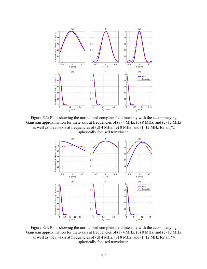
Figure E.3: Plots showing the normalized complete field intensity with the accompanying
Gaussian approximation for the z-axis at frequencies of (a) 4 MHz, (b) 8 MHz, and (c) 12 MHz as well as the rρ-axis at frequencies of (d) 4 MHz, (e) 8 MHz, and (f) 12 MHz for an f/2
spherically focused transducer.
Figure E.4: Plots showing the normalized complete field intensity with the accompanying
Gaussian approximation for the z-axis at frequencies of (a) 4 MHz, (b) 8 MHz, and (c) 12 MHz as well as the rρ-axis at frequencies of (d) 4 MHz, (e) 8 MHz, and (f) 12 MHz for an f/4
spherically focused transducer.
202

Figure E.5: Plot showing the values of G from a complete f/4 source (x) normalized with
respect to the complete G at 8 MHz with a line showing the ideal values of G from Equation (2.38) also normalized with respect to the ideal G at 8 MHz.
o2
o2
o2
o2
Having identified the predominance of the shifts of the focus with frequency, the next
step is to determine if the Gaussian approximation could be improved by properly accounting for
the shift. Since the shift is always along the beam axis, Equation (2.54) could be modified to
yield
ds g s e e ds g s e e
e ds g s e e
z win z
s z fw s
L
L
z win z
sw
s z fw
z fw s
L
L
z fw
z win z
sw
z fw
s
L
L
z oF
z z
z
z
z oF
z
oF
z z
oF
z
z
z
oF
zz
b g b g
b g
b gc h b g b g
b g b g
−−
−
− + −
−
− − +FHG
IKJ
−
F
HGG
I
KJJ =
FHGG
IKJJ
=FHGG
IKJJ
z z
z
4
4
2
2 4 8 44
2
2
4 4 48
2
2
2
21
2
2 2
2
21
2
2
2
2 1 2
α α
α
/
/
/
/
/
/
,
(E.5)
where, in this case, zoF is the shift of the focus at a particular frequency. However, the shift of
the focus is typically much smaller than wz. Hence, the terms involving zoF can be ignored
resulting in the same generalized attenuation-compensation function given in Equation (2.51).
Therefore, the Gaussian approximation could be improved for weakly focused sources provided
the equivalent Gaussian depth of focus is found by an independent fit to a Gaussian distribution
for every frequency of interest while allowing the peak of the Gaussian to occur at different
spatial locations for each frequency. Hence, when finding the Gaussian depth of focus for the
203
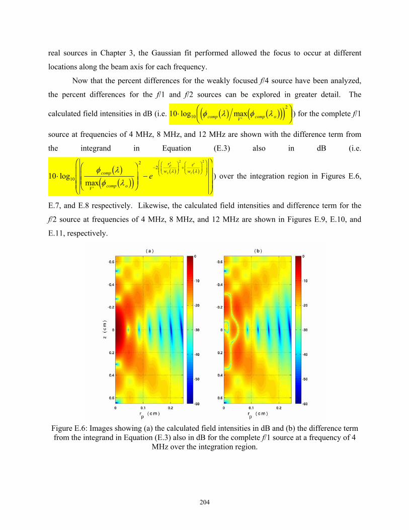
real sources in Chapter 3, the Gaussian fit performed allowed the focus to occur at different
locations along the beam axis for each frequency.
Now that the percent differences for the weakly focused f/4 source have been analyzed,
the percent differences for the f/1 and f/2 sources can be explored in greater detail. The
calculated field intensities in dB (i.e. 10 ) for the complete f/1
source at frequencies of 4 MHz, 8 MHz, and 12 MHz are shown with the difference term from
the integrand in Equation (E.3) also in dB (i.e.
10
2⋅ FHG
IKJ′
log maxφ λ φ λcomp V comp ob g b gde ij
10 10
22
2 2
⋅FHGG
IKJJ −
F
HGGG
I
KJJJ′
−′F
HGIKJ +
′FHG
IKJ
FHGG
IKJJ
logmax
φ λφ λ
ρ
λ λcomp
V comp o
rw
zw
e x zb gb gd i
b g b g) over the integration region in Figures E.6,
E.7, and E.8 respectively. Likewise, the calculated field intensities and difference term for the
f/2 source at frequencies of 4 MHz, 8 MHz, and 12 MHz are shown in Figures E.9, E.10, and
E.11, respectively.
Figure E.6: Images showing (a) the calculated field intensities in dB and (b) the difference term from the integrand in Equation (E.3) also in dB for the complete f/1 source at a frequency of 4
MHz over the integration region.
204
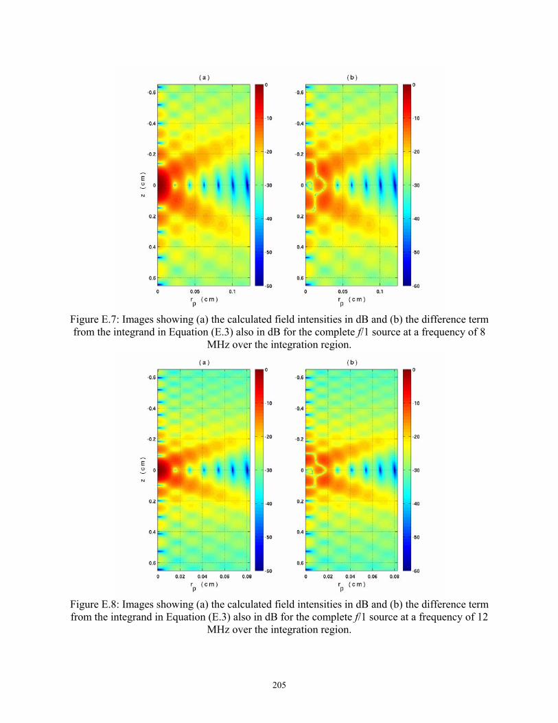
Figure E.7: Images showing (a) the calculated field intensities in dB and (b) the difference term from the integrand in Equation (E.3) also in dB for the complete f/1 source at a frequency of 8
MHz over the integration region.
Figure E.8: Images showing (a) the calculated field intensities in dB and (b) the difference term from the integrand in Equation (E.3) also in dB for the complete f/1 source at a frequency of 12
MHz over the integration region.
205

Figure E.9: Images showing (a) the calculated field intensities in dB and (b) the difference term from the integrand in Equation (E.3) also in dB for the complete f/2 source at a frequency of 4
MHz over the integration region.
Figure E.10: Images showing (a) the calculated field intensities in dB and (b) the difference term
from the integrand in Equation (E.3) also in dB for the complete f/2 source at a frequency of 8 MHz over the integration region.
206

Figure E.11: Images showing (a) the calculated field intensities in dB and (b) the difference term from the integrand in Equation (E.3) also in dB for the complete f/2 source at a frequency of 12
MHz over the integration region.
The largest differences between the complete fields and Gaussian approximations in
Figures E.6 through E.11 (i.e., (b) images) result from the “V” shaped side lobe structure before
and after the focal plane. When very little of this side lobe structure is included in the integration
region (Figure E.9); the corresponding percent difference in Figure E.1a is 3.3%. However,
when all of the “V” is included in the integration region (Figures E.7 and E.8), the corresponding
percent difference in Figure E.1a is close to 18%. Hence, the side lobe structure reduces the
accuracy of the Gaussian approximation for focused sources up to a percent difference of ~18%.
One way to improve the agreement between the complete fields and Gaussian approximation for
focused sources is to use smaller window lengths to gate the time domain signal so that not all of
the “V” shaped side lobe structure would influence the backscattered power spectrum.
207

APPENDIX F: EXAMPLE AVERAGE SQUARED DIFFERENCE CONTOURS
FOR SPECTRAL FIT ALGORITHM
This appendix contains 40 example Average Squared Difference (ASD) contours as given
by Equation (5.3) for different input values of scatterer size and total attenuation. In Figures F.1-
F.8, the colors correspond to the 1/ASD values. Hence, dark red corresponds to a small ASD
value and dark blue corresponds to a large ASD value. The 40 contours correspond to 1000
independent waveforms grouped into sets containing 25 waveforms that were subsequently
averaged in the normal spectral domain. The waveforms were generated for a f/4, 5 cm focal
length source whose filtering characteristics were given by Equation (4.19) sonifying an infinite
half-space with an attenuation of 0.3 dB/cm/MHz containing Gaussian scatterers with effective
radii of 25 µm at a density of 35/mm3. A hamming window with a length of 2.5 mm was used to
gate the time-domain waveforms. Normally, the Spectral Fit algorithm would yield the scatterer
size and total attenuation corresponding to the minimum of these ASD contours. Hence, the
scatterer size yielded by the minimization routine is provided above the corresponding contour.
(a) (b)
Figure F.1: (a) 1st set of 25 waveforms, aeff = 26.619 µm, (b) 2nd set of 25 waveforms, aeff =
24.383 µm.
208
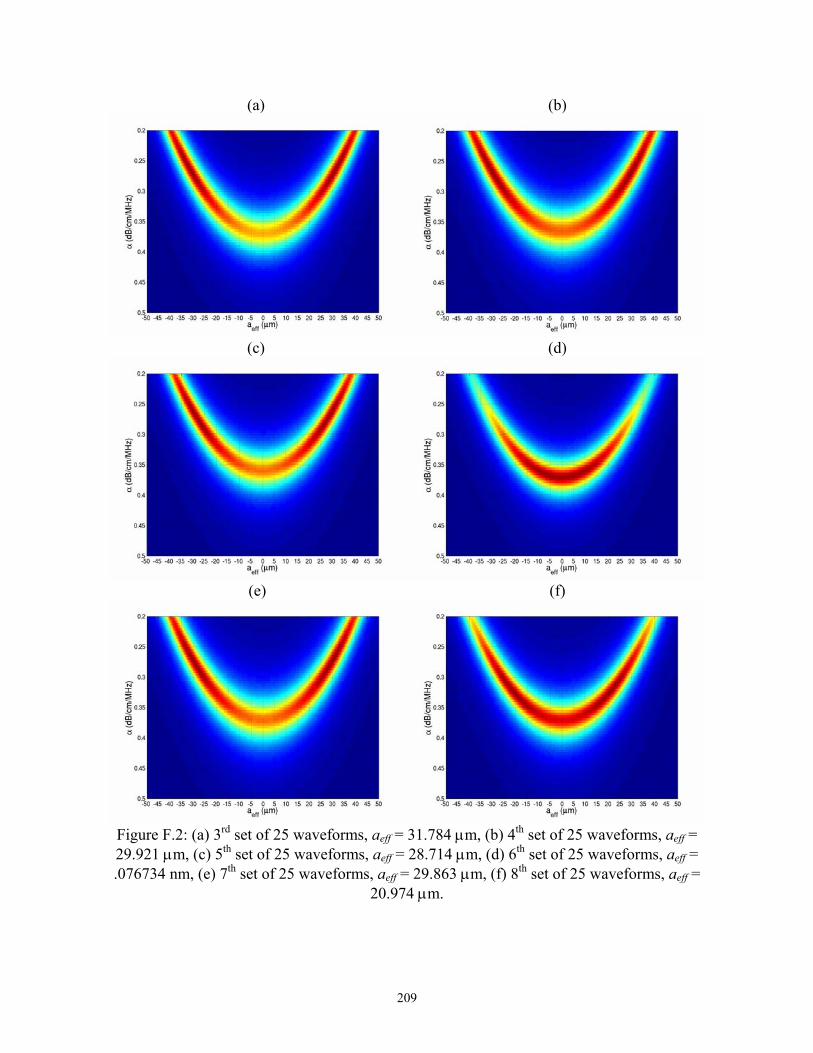
(a) (b)
(c) (d)
(e) (f)
Figure F.2: (a) 3rd set of 25 waveforms, aeff = 31.784 µm, (b) 4th set of 25 waveforms, aeff = 29.921 µm, (c) 5th set of 25 waveforms, aeff = 28.714 µm, (d) 6th set of 25 waveforms, aeff = .076734 nm, (e) 7th set of 25 waveforms, aeff = 29.863 µm, (f) 8th set of 25 waveforms, aeff =
20.974 µm.
209

(a) (b)
(c) (d)
(e) (f)
Figure F.3: (a) 9th set of 25 waveforms, aeff = .019431 nm, (b) 10th set of 25 waveforms, aeff = 37.621 µm, (c) 11th set of 25 waveforms, aeff = 33.909 µm, (d) 12th set of 25 waveforms, aeff = .00730 nm, (e) 13th set of 25 waveforms, aeff = 24.294 µm, (f) 14th set of 25 waveforms, aeff =
25.493 µm.
210
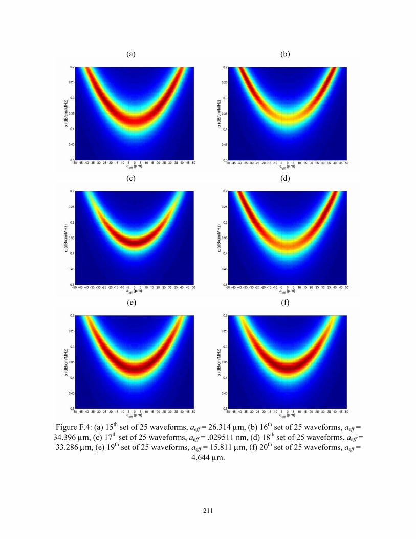
(a) (b)
(c) (d)
(e) (f)
Figure F.4: (a) 15th set of 25 waveforms, aeff = 26.314 µm, (b) 16th set of 25 waveforms, aeff =
34.396 µm, (c) 17th set of 25 waveforms, aeff = .029511 nm, (d) 18th set of 25 waveforms, aeff = 33.286 µm, (e) 19th set of 25 waveforms, aeff = 15.811 µm, (f) 20th set of 25 waveforms, aeff =
4.644 µm.
211
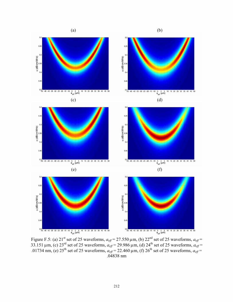
(a) (b)
(c) (d)
(e) (f)
Figure F.5: (a) 21st set of 25 waveforms, aeff = 27.550 µm, (b) 22nd set of 25 waveforms, aeff = 33.151 µm, (c) 23rd set of 25 waveforms, aeff = 29.986 µm, (d) 24th set of 25 waveforms, aeff = .01734 nm, (e) 25th set of 25 waveforms, aeff = 22.460 µm, (f) 26th set of 25 waveforms, aeff =
.04838 nm
212
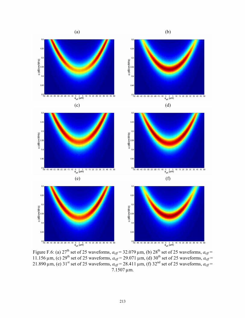
(a) (b)
(c) (d)
(e) (f)
Figure F.6: (a) 27th set of 25 waveforms, aeff = 32.079 µm, (b) 28th set of 25 waveforms, aeff = 11.156 µm, (c) 29th set of 25 waveforms, aeff = 29.071 µm, (d) 30th set of 25 waveforms, aeff = 21.890 µm, (e) 31st set of 25 waveforms, aeff = 28.411 µm, (f) 32nd set of 25 waveforms, aeff =
7.1507 µm.
213
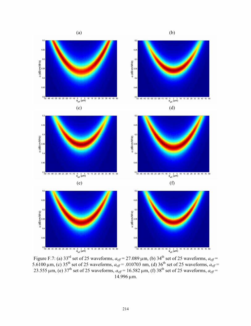
(a) (b)
(c) (d)
(e) (f)
Figure F.7: (a) 33rd set of 25 waveforms, aeff = 27.089 µm, (b) 34th set of 25 waveforms, aeff =
5.6100 µm, (c) 35th set of 25 waveforms, aeff = .010703 nm, (d) 36th set of 25 waveforms, aeff = 23.555 µm, (e) 37th set of 25 waveforms, aeff = 16.582 µm, (f) 38th set of 25 waveforms, aeff =
14.996 µm.
214

(a) (b)
Figure F.8: (a) 39th set of 25 waveforms, aeff = 23.843 µm, (b) 40th set of 25 waveforms, aeff =
26.275 µm.
215
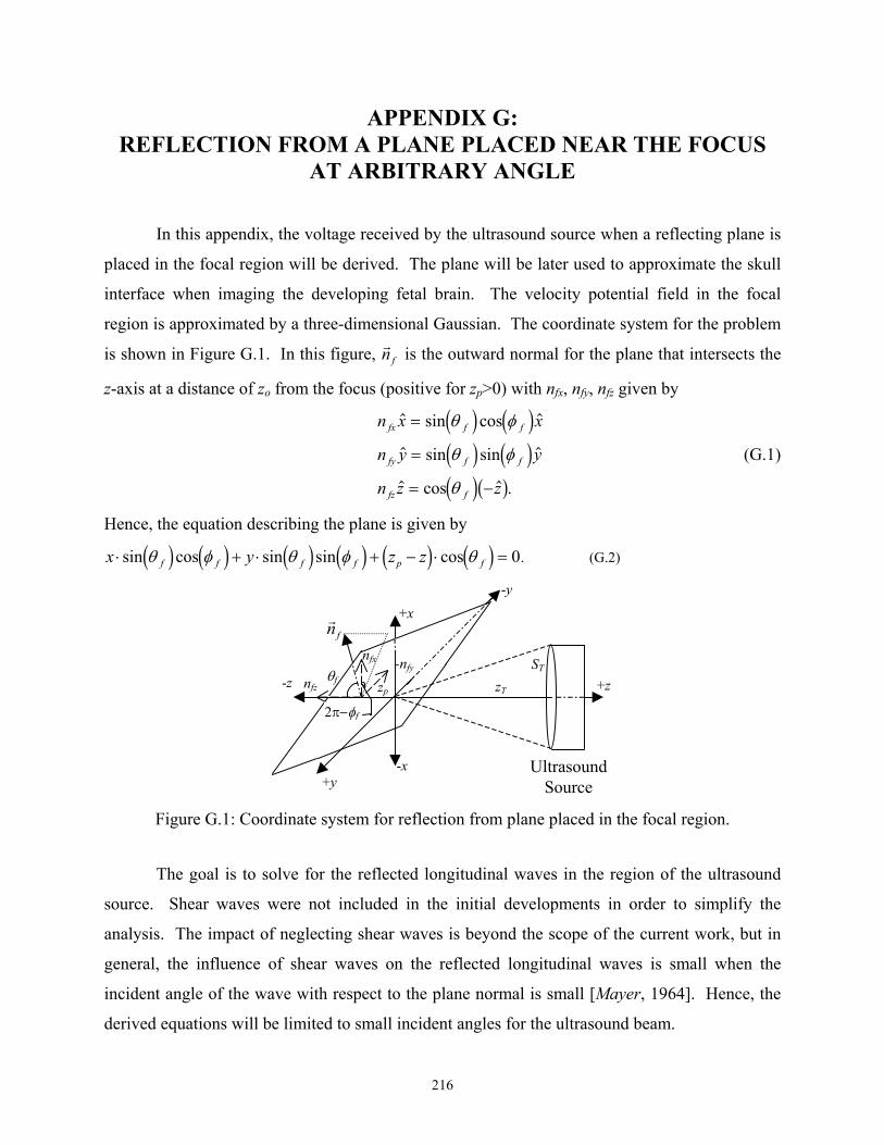
APPENDIX G: REFLECTION FROM A PLANE PLACED NEAR THE FOCUS
AT ARBITRARY ANGLE In this appendix, the voltage received by the ultrasound source when a reflecting plane is
placed in the focal region will be derived. The plane will be later used to approximate the skull
interface when imaging the developing fetal brain. The velocity potential field in the focal
region is approximated by a three-dimensional Gaussian. The coordinate system for the problem
is shown in Figure G.1. In this figure, n is the outward normal for the plane that intersects the
z-axis at a distance of z
f
o from the focus (positive for zp>0) with nfx, nfy, nfz given by
n x x
n y y
n z z
fx f f
fy f f
fz f
sin cos
sin sin
cos .
=
=
= −
θ φ
θ φ
θ
d i d id i d id ib g
(G.1)
Hence, the equation describing the plane is given by
x y z zf f f f p f⋅ + ⋅ + − ⋅sin cos sin sin cosθ φ θ φ θd i d i d i d i d i d i 0= . (G.2)
nf
+z-z
-x
+x
+y
-y
zT
ST
UltrasoundSource
nfx -nfy
nfzθf
2π−φf
zp
Figure G.1: Coordinate system for reflection from plane placed in the focal region.
The goal is to solve for the reflected longitudinal waves in the region of the ultrasound
source. Shear waves were not included in the initial developments in order to simplify the
analysis. The impact of neglecting shear waves is beyond the scope of the current work, but in
general, the influence of shear waves on the reflected longitudinal waves is small when the
incident angle of the wave with respect to the plane normal is small [Mayer, 1964]. Hence, the
derived equations will be limited to small incident angles for the ultrasound beam.
216
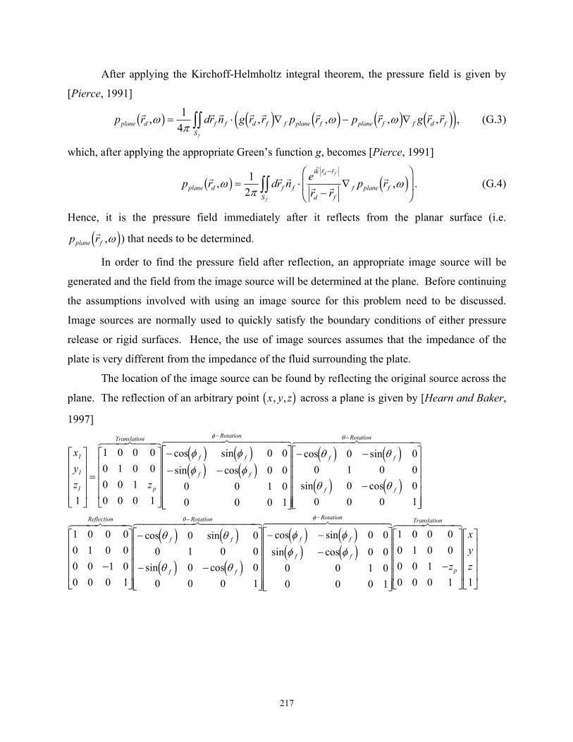
After applying the Kirchoff-Helmholtz integral theorem, the pressure field is given by
[Pierce, 1991]
p r dr n g r r p r p r g r rplane d f f d f f plane f plane f f d fS f
, , , ,ωπ
ω ωb g d i d i d i de j= ⋅ ∇ − ∇zz14
, i , (G.3)
which, after applying the appropriate Green’s function g, becomes [Pierce, 1991]
p r dr n er r
p rplane d f f
ik r r
d ff plane f
S
d f
f
, ,~
ωπ
ωb g d= ⋅−
∇ iFHG
IKJ
−
zz12
. (G.4)
Hence, it is the pressure field immediately after it reflects from the planar surface (i.e.
) that needs to be determined. p rplane f ,ωd i
g
In order to find the pressure field after reflection, an appropriate image source will be
generated and the field from the image source will be determined at the plane. Before continuing
the assumptions involved with using an image source for this problem need to be discussed.
Image sources are normally used to quickly satisfy the boundary conditions of either pressure
release or rigid surfaces. Hence, the use of image sources assumes that the impedance of the
plate is very different from the impedance of the fluid surrounding the plate.
The location of the image source can be found by reflecting the original source across the
plane. The reflection of an arbitrary point b across a plane is given by [Hearn and Baker,
1997]
x y z, ,
xyz z
I
I
I p
Translation
f f
f f
Rotation
f f
f f
Rotation
1
1 0 0 00 1 0 00 0 10 0 0 1
0 00 0
0 0 1 00 0 0 1
0 00 1 0 0
0 00 0 0 1
L
N
MMMM
O
Q
PPPP=
L
N
MMMM
O
Q
PPPP
−
− −
L
N
MMMMM
O
Q
PPPPP
− −
−
L
N
MMMMM
O
Q
PPPPP
− −
cos sinsin cos
cos sin
sin cos
φ φφ φ
θ θ
θ θ
φ θ
d i d id i d i
d i d i
d i d i
1 0 0 00 1 0 00 0 1 00 0 0 1
0 00 1 0 0
0 00 0 0 1
0 00 0
0 0 1 00 0 0 1
1
−
L
N
MMMM
O
Q
PPPP
−
− −
L
N
MMMMM
O
Q
PPPPP
− −
−
L
N
MMMMM
O
Q
PPPPP
− −Reflection
cos sin
sin cos
cos sinsin cos
θ θ
θ θ
φ φφ φ
θ φ
f f
f f
Rotation
f f
f f
Rotation
d i d i
d i d i
d i d id i d i
0 0 00 1 0 00 0 10 0 0 1 1
−
L
N
MMMM
O
Q
PPPP
L
N
MMMM
O
Q
PPPPz
xyzp
Translation
217
=
L
N
MMMM
O
Q
PPPP−
−
L
N
MMMMM
O
Q
PPPPP−
L
N
MMMM
O
Q
PPPP
−
1 0 0 00 1 0 00 0 10 0 0 1
00
0 00 0 0 1
1 0 0 00 1 0 00 0 1 00 0 0 1
0
zp
f f f f f
f f f f f
f f
f f f f f
f f
cos cos sin sin cossin cos cos sin sin
sin cos
cos cos sin cos sinsin cos
φ θ φ θ φφ θ φ θ φ
θ θ
φ θ φ θ θφ φ
d i d i d i d i d id i d i d i d i d id i d i
d i d i d i d i d id i d id i d i d i d i d i
0 00
0 0 0 1
1 0 0 00 1 0 00 0 10 0 0 1 1
sin cos sin sin cosθ φ θ φ θf f f f f pz
xyz−
L
N
MMMMM
O
Q
PPPPP−
L
N
MMMM
O
Q
PPPP
L
N
MMMM
O
Q
PPPP
=
− −
− −
−
L
N
MMMMM
O
Q
PPPPP
1 2 2 2 0
2 1 2 2
2 2 1 20 0 0
1 0 0 00 1 0 00
2 2 2
2 2 2
2
sin cos sin sin cos sin cos cos
sin sin cos sin sin sin sin cos
sin cos cos sin sin cos cos
θ φ θ φ φ θ φ θ
θ φ φ θ φ θ φ θ
θ φ θ θ φ θ θ
f f f f f f f f
f f f f f f f f
f f f f f f f z
d i d ie j d i d i d i d i d i d id i d i d i d i d ie j d i d i d id i d i d i d i d i d i d ie j
0 10 0 0 1 1 0 0 0 1 1 1
1 1 1 2 1 3 1 4
2 1 2 2 2 3 2 4
3 1 3 2 3 3 3 4−
L
N
MMMM
O
Q
PPPP
L
N
MMMM
O
Q
PPPP=
L
N
MMMM
O
Q
PPPP
L
0
1p
N
MMMM
O
Q
PPPP=
L
N
MMMM
O
Q
PPPPz
xyz
xyz
xyzp
M M M MM M M MM M M M
M
image image image image
image image image image
image image image imageimage
, , , ,
, , , ,
, , , , ,
(G.5)
where
M M
M
image image
image
:,
sin cos
sin sin cossin cos cos
:,
sin sin cos
sin sin
sin sin cos
:,
sin cos cossin
1
1 2
22
0
2
2
1 2
20
3
22
2 2
2
2
2 2
b gd i d ie j
d i d i d id i d i d i
b gd i d i d id i d ie j
d i d i d i
b gd i d i d id
=
−
−
L
N
MMMMM
O
Q
PPPPP=
−
−
L
N
MMMMM
O
Q
PPPPP
=
θ φ
θ φ φθ φ θ
θ φ φ
θ φ
θ φ θ
θ φ θθ
f f
f f f
f f f
f f
f f
f f f
f f f
f i d i d id ie j
b gd i d i d id i d i d id i
sin cos
cos:,
sin cos cossin sin cos
cosφ θ
θ
θ φ θθ φ θ
θf f
f
p f f f
p f f f
p f
zz
z1 20
4
22
21
2 2−
L
N
MMMMM
O
Q
PPPPP=
−
−
L
f
N
MMMMM
O
Q
PPPPPMimage
(G.6)
and is the image of the original point. Therefore, the field from the image source
would be given by [Pierce, 1991]
x y zI I I, ,b g
218
p r dr n er r
p r i dr n er r
u r
i K V Hdr G r e
r r
plane f I I
ik r r
I fI plane I
SI I
ik r r
I fI
S
plane uV incI T I
ik r r
I fS
I f
I
I f
I
I f
I
, ,
, ,
~ ~
~
ωπ
ω ωρπ
ω
ωρΓ ω ω ωπ
ω
d i b g b g
b g b g b g b g
=−
⋅−
∇ ,FHG
IKJ=−
⋅−
FHG
IKJ
=−
−
− −
−
zz zzzz
12 2
2
(G.7)
where Γplane accounts for the fact that the plane may not be a perfect reflector, and nI is the
normal vector perpendicular to the aperture plane of the image source pointing away from the
direction of wave propagation. Note that Γplane is only intended to correct for small deviations
from a perfect reflector. Large deviations are not allowed under the current method of images
formulation. Also, assuming that the planar surface is near the focus (i.e., rf is small compared
to rI ), Equation (G.7) becomes
p ri K V H
dr G r er
eplane fplane uV inc
I T I
ikr
I
ik rr
r
S
I I
If
I
, ,~ ~
ωωρΓ ω ω ω
πωd i b g b g b g b g≅
− − ⋅zz2, (G.8)
which can be written in closed form if the velocity potential field near the focus can be
approximated as a three-dimensional Gaussian. Hence, Equation (G.8) becomes
p ri K V H G
eplane fplane uV inc o w w w ik z
x
x
y
y
z
zT z,
~ω
ωρΓ ω ω ωe
π
ξ ξ ξ
ξd i b g b g b g b≅− −
gFHGIKJ +FHGIKJ +FHGIKJ
FHGG
IKJJ −
2
2 2 2
, (G.9)
where d refer to the coordinate system for the image source and zξ ξ ξx y z, , i
i
i
T is also the distance
of the aperture plane of the image source from its focus (same as for the original source).
The locations of points d now need to be determined in the original coordinate
system. Because the ξ
ξ ξ ξx y z, ,
x-axis, ξy-axis, and ξz-axis are the image of the x-axis, y-axis, and z-axis,
Equation (G.5) yields ,
,
,
,
,
,
,
,
,
ξ
ξ
ξ
ξ
ξ
ξ
ξ
ξ
ξ
x
x
x
y
y
y
z
z
z
x
y
z
x
y
z
x
y
z
⋅ =
⋅ =
⋅ =
⋅ =
⋅ =
⋅ =
⋅ =
⋅ =
⋅ =
M
M
M
M
M
M
M
M
M
image
image
image
image
image
image
image
image
image
1 1
2 1
3 1
1 2
2 2
2 3
1 3
2 3
3 3
, (G.10)
and the origin of the d coordinate system is located at d i. Therefore, d i in b coordinates are given by
ξ ξ ξx y z, ,
x y z, , gM M Mimage image image
1 4 2 4 3 4, , ,, ,
ξ ξ ξx y z, ,
219
ξ
ξ
ξ
x
y
z
x y z
x y z
x y z
= + + +
= + + +
= + + +
M M M M
M M M M
M M M M
image image,
image image
image,
image image image
image,
image image image
1 1 2 1 3 1 1 4
1 2 2 2 3 2 2 4
1 3 2 3 3 3 3 4
, ,
, ,
, ,
,
,
,
i
(G.11)
providing an expression for in closed form. p rplane f ,ωd Now determine n p by taking the gradient of Equation (G.9) to yield rf f plane f⋅∇ ,ωd i
∇ ≅−
∇
F
HGGG
I
KJJJ
−FHGIKJ +FHGIKJ +FHGIKJ
FHGG
IKJJ −
f plane fplane uV inc o
f
w w w ik zp ri K V H G
e ex
x
y
y
z
zT z,
~ω
ωρΓ ω ω ωπ
ξ ξ ξ
ξd i b g b g b g b g2
2 2 2
=−
F
HGGG
I
KJJJ
∇ − −FHGIKJ +FHGIKJ +FHGIKJ
FHGG
IKJJ
FHGG
IKJJ
−FHGIKJ +FHGIKJ +FHGIKJ
FHGG
IKJJ −i K V H G
e e
ik zw w w
plane uV inc o w w w ik z
f T zx
x
y
y
z
z
x
x
y
y
z
zT z
ωρΓ ω ω ωπ
ξ ξ ξ ξ
ξ ξ ξ
ξb g b g b g
b g
b g2
2 2 2
2 2 2
~
~
=
F
HGGG
I
KJJJ
∇ +FHGIKJ +FHGIKJ +FHGIKJ
FHGG
IKJJ
−FHGIKJ +FHGIKJ +FHGIKJ
FHGG
IKJJ −i K V H G
e e
ikw w w
plane uV inc o w w w ik z
f zx
x
y
y
z
z
x
x
y
y
z
zT z
ωρΓ ω ω ωπ
ξ ξ ξ ξ
ξ ξ ξ
ξb g b g b g b g2
2 2 2
2 2 2
~
~
=
F
HGGG
I
KJJJ
∇ + ∇ + ∇ + ∇FHG
IKJ
−FHGIKJ +FHGIKJ +FHGIKJ
FHGG
IKJJ −i K V H G
e e
ikw w w
plane uV inc o w w w ik z
f zx
xf x
y
yf y
z
zf z
x
x
y
y
z
zT z
ωρΓ ω ω ωπ
ξξ
ξξ
ξξ
ξ
ξ ξ ξ
ξb g b g b g b g2
2 2 2
2 2 2
~
~ .
(G.12)
Now taking the derivative of the expressions given in Equation (G.11) for ξx, ξy, and ξz yields
∇ =
L
NMMM
O
QPPP
∇ =
L
NMMM
O
QPPP
∇ =
L
NMMM
O
QPPP
f x f y f zξ ξ ξMMM
MMM
MMM
image
image,
image
image
image,
image
image
image,
image
1 1
2 1
3 1
1 2
2 2
3 2
1 3
2 3
3 3
,
,
,
,
,
,
. (G.13)
Also, taking the dot product of the expressions in Equation (G.13) with n yields f
220
n
n
n
f f x f f f f f
f f y f f f f f
f f z f f f f f
⋅∇ = + −
⋅∇ = + −
⋅∇ = + −
ξ θ φ θ φ
ξ θ φ θ φ
ξ θ φ θ φ
M M M
M M M
M M M
image image,
image
image image,
image
image image,
image
1 1 2 1 3 1
1 2 2 2 3 2
1 3 2 3 3 3
, ,
, ,
, ,
sin cos sin sin cos
sin cos sin sin cos
sin cos sin sin cos .
d i d i d i d i d id i d i d i d i dd i d i d i d i d i
θ
θ
θ
i (G.14)
At this point, the results can be simplified by assuming that θf is less than π/6, the typical critical
angle for longitudinal waves going from tissue to bone [Fujii et al., 1999]. Larger angles would
result in no signal entering the brain and, consequently, no image of the brain could be formed.
Also, a small incident angle is required if the neglecting of shear waves is going to be valid
[Mayer, 1964]. Under this assumption, 2 ξ ξx
xf xw
∇ , 2ξ
ξy
yf yw
∇ , and 2 ξ ξz
zf zw
∇ are all small
compared to ik f z~∇ ξ . Hence, n p can be approximated as rf f plane f⋅∇ ,ωd i
n p rk K V H G
e e nf f plane fplane uV inc o w w w ik z
f f z
x
x
y
y
z
zT z⋅∇ ≅
−F
HGGG
I
KJJJ
⋅∇−FHGIKJ +FHGIKJ +FHGIKJ
FHGG
IKJJ −,
~~
ωωρΓ ω ω ω
πξ
ξ ξ ξ
ξd i b g b g b g d ib g2
2 2 2
=−
F
HGGG
I
KJJJ
−FHGIKJ +FHGIKJ +FHGIKJ
FHGG
IKJJ −
~cos
~k K V H Ge eplane uV inc o w w w ik z
f
x
x
y
y
z
zT z
ωρΓ ω ω ωπ
θ
ξ ξ ξ
ξb g b g b g db g2
2 2 2
i . (G.15)
Now that an expression for n p has been derived, rf f plane f⋅∇ ,ωd i p rplane d ,ωb g can be
found from Equation (G.4). Substituting in for the necessary parameters yields
p r dr er r
n p r
k K V H Gdr e
r re e
plane d f
ik r r
d ff f plane f
S
plane uV inc o ff
ik r r
d f
w w w ik z
S
d f
f
d fx
x
y
y
z
zT z
f
, ,
~ cos,
~
~~
ωπ
ω
ωρΓ ω ω ω θ
π
ξ ξ ξ
ξ
b g d ie j
b g b g b g d ib g
b g
=−
⋅∇
=−
−
F
HGGG
I
KJJJ
−
− −FHGIKJ +FHGIKJ +FHGIKJ
FHGG
IKJJ −
zz
zz
12
2 2
2 2 2
(G.16)
where ξx, ξy, and ξz are given by Equation (G.11).
After determining the reflected fields in the region containing the original ultrasound
source, these fields need to be translated to a voltage output by the transducer. The voltage
output by the source can be found from
221
VH
i S Kdr G r
pzplane
T uVd T d
S
plane
dT
ωω
ωρ ωωb g b g
b g b g=∂
∂zz , , (G.17)
where ∂ ∂p zplane d is given by
∂∂
=−
⋅
F
HGGG
I
KJJJ
∂∂ −
−FHGIKJ +FHGIKJ +FHGIKJ
FHGG
IKJJ −
−
zzz
p rk K V H G
dr e ez
er r
dplane d
plane uV inc o f
f
w w w ik z
d
ik r r
d fS
x
x
y
y
z
zT z
d f
f
,~ cos
~~
ωωρΓ ω ω ω θ
π
ξ ξ ξ
ξ
b g b g b g b g d ib g
b g
2 2
2 2 2
≅−
⋅
F
HGGG
I
KJJJ
−FHGIKJ +FHGIKJ +FHGIKJ
FHGG
IKJJ −
− ⋅zz
~ cos
~~
~ ~
k K V H G
dr e e ikzr
e
plane uV inc o f
f
w w w ik z d
d
ikr ikr rr
S
x
x
y
y
z
zT z
d fd
d
f
ωρΓ ω ω ω θ
π
ξ ξ ξ
ξ
b g b g b g d ib g
b g
2 2
2
2 2 2
≅−
⋅
F
HGGG
I
KJJJ
−FHGIKJ +FHGIKJ +FHGIKJ
FHGG
IKJJ −
− ⋅
zz
ik K V H G
dr e e er
plane uV inc o f
f
w w w ik z
ikr ikrrr
dS
x
x
y
y
z
zT z
d fd
d
f
~ cos
.~
~ ~
2
222 2 2
ωρΓ ω ω ω θ
π
ξ ξ ξ
ξ
b g b g b g d ib g
b g (G.18)
Hence, the reflected voltage from the plate is given by
Vk V H G
S
dr G r dr e e er
planeplane inc o f
T
d T dS
f
w w w ik z
ikr ik r rr
dST
x
x
y
y
z
zT z
d fd
d
f
ωω ω θ
π
ωξ ξ ξ
ξ
b g b g b g d ib g
b g b g
≅−
⋅
F
HGGG
I
KJJJzz zz
−FHGIKJ +FHGIKJ +FHGIKJ
FHGG
IKJJ −
− ⋅
~ cos
,~
~ ~
2 2
222 2 2
Γ
=−
⋅F
HGGG
I
KJJJ
F
HGGG
I
KJJJ
−FHGIKJ +FHGIKJ +FHGIKJ
FHGG
IKJJ −
− ⋅
zzzz
~ cos
,~
~ ~
k V H G
S
dr e e dr G r er
plane inc o f
T
f
w w w ik zd T d
S
ikr ikr rr
dS
x
x
y
y
z
zT z
T
d fd
d
f
2 2
222 2 2
Γ ω ω θ
π
ωξ ξ ξ
ξ
b g b g d ib g
b gb g
222
=−
⋅
F
HGGG
I
KJJJ
F
HGGG
I
KJJJ
−FHGIKJ +FHGIKJ +FHGIKJ
FHGG
IKJJ −
−FHGIKJ +FHGIKJ +FHGIKJ
FHGG
IKJJ −zz
~ cos
~ ~
k V H G
S
dr e e e e
plane inc o f
T
f
w w w ik z
xw
yw
zw ik z z
S
x
x
y
y
z
zT z
f
x
f
y
f
z T f
f
2 2 2
222 2 2 2 2 2
Γ ω ω θ
π
ξ ξ ξ
ξ
b g b g d ib g
b g d i
=F
HGG
I
KJJ
−+
++
++
+ +FHG
IKJzzΩ ω
ξ ξ ξξ
b gd i
dr ef
x
w
y
w
z
wik z
S
x f
x
y f
y
z f
zz f
f
2 2
2
2 2
2
2 2
2~
, (G.19)
where the velocity potential fields has been assumed to be Gaussian and Ω ωb g is given by
ΩΓ
ωω ω θ
πb g b g b g d i
b g=−~ cos ~k V H G
Seplane inc o f
T
i kzT
2 2 2
22
2. (G.20)
In order to integrate Equation (G.19), all of the spatial coordinates need to be expressed in terms
of xf and yf. Solving Equations (G.11) and (G.2) yields
ξ x f f f
f f f f f f f
f f
x y z
x y x z x y z
y z
2 2 1 1 1 1 2 2 1 2 1 2 3 1 3 1 1 4 1 4
1 1 2 1 1 1 3 1 1 1 1 4 2 1 3 1
2 1 1 4 3 1 1 4
2 2 2 2
2 2
= + + +
+ + + +
+ +
M M M M M M M M
M M M M M M M M
M M M M
image image image,
image,
image image image image
image image,
image image image image image,
image
image,
image image image
, , , , , ,
, , , , ,
, , ,
,
ξ y f f f
f f f f f f f
f f
x y z
x y x z x y z
y z
2 2 1 2 1 2 2 2 2 2 2 2 3 2 3 2 2 4 2 4
1 2 2 2 1 2 3 2 1 2 2 4 2 2 3 2
2 2 2 4 3 2 2 4
2 2 2 2
2 2
= + + +
+ + + +
+ +
M M M M M M M M
M M M M M M M M
M M M M
image image image,
image,
image image image image
image image,
image image image image image,
image
image,
image image image
, , , , , ,
, , , , ,
, , ,
,
ξ z f f f
f f f f f f f
f f
x y z
x y x z x y z
y z
2 2 1 3 1 3 2 2 3 2 3 2 3 3 3 3 3 4 3 4
1 3 2 3 1 3 3 3 1 3 3 4 2 3 3 3
2 3 3 4 3 3 3 4
2 2 2 2
2 2
= + + +
+ + + +
+ +
M M M M M M M M
M M M M M M M M
M M M M
image image image,
image,
image image image image
image image,
image image image image image,
image
image,
image image image
, , , , , ,
, , , , ,
, , ,
,
p
f
(G.21)
and
z x y z
x C y C z
z x C x y C C x z C y C y z C z
f f f f f f f p
f f p
f f f f f p f f p
= ⋅ + ⋅ +
= + +
⇒ = + + + + +
tan cos tan sin
,
θ φ θ φd i d i d i d i1 2
2 212
1 2 12
22
222 2 2
(G.22)
where
C
C
f
f f
1
2
=
=
tan cos
tan sin .
θ φ
θ φ
d i d id i d i
(G.23)
223

Now consider each term of the exponent of Equation (G.19) individually.
ik z ikx C C y C C
z zz f
f f
p p
~ ~, ,
, ,ξ + =
+ + + + +
+ + +
,FHGG
IKJJd i d i dM M M M
M Mimage,
image image image
image image
1 31 1
3 3 2 32 2
3 3
3 4 3 3
i (G.24)
ξ x f
xf
x x x x
xw
xw w
Cw
Cw
2 2
22
2
1 1 1 1
2 12
3 1 3 1
2 1
1 1 3 1
2
1 2+
= + + +FHG
IKJ
M M M M M Mimage image image image image image, , , , , ,
++ +
+
F
H
GGGG
I
K
JJJJx
wz C
wC
w
zw
fx
px x
px
2 2 2
2
1 1 1 4
2 1
3 1 3 1
2 1
3 1 1 4
2
1 1 3 1
2
M M M M M M
M M
image image image image image image
image image
, , , , , ,
, ,
+ + +FHG
IKJ
M M M M M Mimage image image image image image1 4 1 4
22
3 1 3 1
2
3 1 1 4
22, , , , , ,
wz
wz
wxp
xp
x
+ + +FHG
IKJ
+
+ +
+ + +
+
yw
Cw
Cw
y
xw w
x C Cw
z Cw
x Cw
x Cw
C
fx x x
f
fx x
fx
px
fx
fx
22 1 2 1
2 22
3 1 3 1
2 2
2 1 3 1
2
1 1 2 1
2
2 1 1 4
2 1 2
3 1 3 1
2
2
3 1 3 1
2 1
2 1 3 1
2 2
1 1 3 1
2
2
2
2 2 2
2 2 2
2
M M M M M M
M M M M M M
M M M M M M
M
image,
image,
image image image,
image
image image,
image,
image image image
image image image,
image image image
, , ,
, , ,
, , , , ,
,
image image image,
imageM M M3 1 1 4
2
2 1 3 1
22, , ,
wz
wxp
x
+
F
H
GGGGGGGG
I
K
JJJJJJJJ
(G.25)
ξ y f
yf
y y
fy
py y
py
yw
xw
Cw
Cw
xw
z Cw
Cw
zw
2 2
22
1 2 1 2
2 12
3 2 3 2
2 1
1 2 3 2
2
1 2 2 4
2 1
3 2 3 2
2 1
3 2 2 4
2
1 2 3 2
2
2
2 2 2
2
+= + +
y
FHG
IKJ
+
+ +
+
F
H
GGGGG
I
K
JJJJJ
M M M M M M
M M M M M M
M M
image image image image image image
image image image image image image
image image
, , , , , ,
, , , , , ,
, ,
+ + +FHG
IKJ
M M M M M Mimage image image image image image2 4 2 4
22
3 2 3 2
2
3 2 2 4
22, , , , , ,
wz
wz
wyp
yp
y
+ + + +FHG
IKJy
w wC
wC
wfy y y y
22
2 2 2 2
2 22
3 2 3 2
2 2
2 2 3 2
2
1 2M M M M M Mimage
,image
,image image image
,image
, , ,
224
+
+ +
+ + +
+ +
F
H
GGGGGGGG
I
K
JJJJJJJJ
y
xw w
x C Cw
z Cw
x Cw
x Cw
Cw
zw
f
fy y
fy
py
fy
fy
yp
y
2 2 2
2 2 2
2 2
1 2 2 2
2
2 2 2 4
2 1 2
3 2 3 2
2
2
3 2 3 2
2 1
2 2 3 2
2 2
1 2 3 2
2
2
3 2 2 4
2
2 2 3 2
2
M M M M M M
M M M M M M
M M M M
image image,
image,
image image image
image image image,
image image image
image image image,
image
, , ,
, , , , ,
, , ,
,
(G.26)
ξ z f
zf
z z z z
fz
p
zp
z
zp
z
zw
xw
Cw
Cw
Cw
xw
z Cw
z Cw
Cw
zw
2 2
22
1 3 1 3
212
2 12
3 3 3 3
2 1
1 3 3 3
2
1 3 3 4
21
2 1
3 3 3 3
2
1
3 3 3 4
2
1 3 3 3
2
2
22
2
2 2
+= + + +FHG
IKJ
++ +
+ +
F
H
GGGG
I
K
JJJJ
M M M M M M
M M M M
M M M M
image image image image image image
image image image image
image image image image
, , , , , ,
, , , ,
, , , ,
+ + + +FHG
IKJ
M M M M M Mimage image image image image image3 4 3 4
2
2
22
3 3 3 3
2
3 3 3 4
22, , , , , ,
wzw
zw
zwz
p
zp
zp
z
+ + + +FHG
IKJ
+
+ +
+ + +
+
yw
Cw
Cw
Cw
y
xw w
x C Cw
x C Cw
z Cw
z Cw
x Cw
fz z z z
f
fz z
f
z
fz
p
zp
z
fz
22 3 2 3
222
2 22
3 3 3 3
2 2
2 3 3 3
2
1 3 2 3
2
2 3 3 4
21 2
2
1 2
3 3 3 3
22
2 2
3 3 3 3
2
1
2 3 3 3
2
2 22
22
2
2
M M M M M M
M M M M
M M M M
M M
image,
image,
image image image,
image
image image,
image,
image
image image image image
image,
image
, , ,
, ,
, , , ,
,
2 2
1 3 3 3
2 2
3 3 3 4
2
2 3 3 3
2
2 2
2
+ +
+
F
H
GGGGGGGGGGG
I
K
JJJJJJJJJJJ
x Cw
Cw
zw
fz z
pz
M M M M
M M
image image image image
image,
image
, , , ,
,
(G.27)
The appropriate terms can then be grouped resulting in an expression for the voltage returned
from the plane given by
225
VCw
Cw
Cw
ikC
dx
xXw
Xw
Xw
xXw
Xw
Xw
ikX
dy
yYw
Yw
Yw
yYw
Yw
Y
planex
x
y
y
z
zk
f
fx
x
y
y
z
z
fx
x
y
y
z
zk
f
fx
x
y
y
z
z
f
x
x
y
y
ω ωb g b g≅ − + + +FHG
IKJ
FHG
IKJ
− + +FHG
IKJ
− + + +FHG
IKJ
F
H
GGGGG
I
K
JJJJJ
− + +FHG
IKJ
−+ +
Ω exp ~
exp~
exp
2 2 2
2 12
12
12
22
22
22
2 12
12
12
22
22
22z
z
k
w
ikY+
F
HGGG
I
KJJJ
F
H
GGGGGGG
I
K
JJJJJJJ
F
H
GGGGGGG
I
K
JJJJJJJ−∞
∞
−∞
∞ zz~
,
(G.28)
where
X C C
Y C C
C z z z
k f
k f
k p p p
= + + =
= + + =
= + + =
M M
M M
M M
image,
image
image image
image image
1 31 1
3 3
2 32 2
3 3
3 4 3 3
2
2
2
,
, ,
, ,
tan cos
tan sin
θ φ
θ φ
d i d id i d i
f
f
=
=
(G.29)
X C C
X z C C zx
x p p
11 1 1 1
12 3 1 3 1
11 1 3 1
21 1 1 4
13 1 3 1
13 1 1 4 1 1 3 1
1 2 2
2 0
= + + + =
= + + +
M M M M M M
M M M M M M M Mimage image image image image image
image image image image image image image image
, , , , , ,
, , , , , , , ,d i (G.30)
X C C
X z C C zy
y p p
11 2 1 2
12 3 2 3 2
11 2 3 2
21 2 2 4
13 2 3 2
13 2 2 4 1 2 3 2
2 0
2 0
= + + =
= + + +
M M M M M M
M M M M M M M Mimage image image image image image
image image image image image image image image
, , , , , ,
, , , , , , , ,d i (G.31)
X C C C
X z C z C C z
z
z
f f
z p p p
p f f
11 3 1 3
12
12 3 3 3 3
11 3 3 3
2 2
21 3 3 4
1 13 3 3 3
13 3 3 4 1 3 3 3
2
2
2
4
= + + +
=
= + + + +
=
M M M M M M
M M M M M M M M
image image image image image image
image image image image image image image image
, , , , , ,
, , , , , , , ,
tan cos
tan cos
θ φ
θ φ
d i d id id i d i
(G.32)
Y C C
Y x C C C C
z C C z
x
x f
p p
12 1 2 1
22 3 1 3 1
22 1 3 1
21 1 2 1
1 23 1 3 1
12 1 3 1
21 1 3 1
2 1 1 42
3 1 3 12
3 1 1 4 2 1 3 1
2 0
2
2 0
= + + =
= + + +
+ + + +
M M M M M M
M M M M M M M M
M M M M M M M M
image,
image,
image image image,
image
image image,
image image image,
image image image
image,
image image image image image image,
image
, , ,
, , , , ,
, , , , , ,
d id i =
, (G.33)
Y C C
Y x C C C C
z C C z
y
y f
p p
12 2 2 2
22 3 2 3 2
22 2 3 2
21 2 2 2
1 23 2 3 2
12 2 3 2
21 2 3 2
2 2 2 42
3 2 3 22
3 2 2 4 2 2 3 2
1 2 2
2
2 0
= + + + =
= + + +
+ + + +
M M M M M M
M M M M M M M M
M M M M M M M M
image,
image,
image image image,
image
image image,
image image image,
image image image
image,
image image image image image image,
image
, , ,
, , , , ,
, , , , , ,
d id i =
, (G.34)
226
Y C C C
Y x C C C C C C
z C z C C z
z
f f
z f
p p p
12 3 2 3
22
22 3 3 3 3
22 3 3 3
2 2
21 3 2 3
1 2 1 23 3 3 3
12 3 3 3
21 3 3 3
2 3 3 42 2
3 3 3 32
3 3 3 4
2
2
2
2
= + + +
=
= + + + +
+ + + + +
M M M M M M
M M M M M M M M
M M M M M M M
image,
image,
image image image,
image
image image,
image image image,
image image image
image,
image image image image image
, , ,
, , , ,
, , , , ,
tan sinθ φd i d id i
image,
imageM2 3 3 3
24 4
,
tan sin cos tan sin
d id i d i d i d i d i= +x zf f f f p f fθ φ φ θ φ
, ,
zp
(G.35)
C z z
C z z
C z z z
x p p
y p p
z p p p
= + + =
= + + =
= + + +
M M M M M M
M M M M M M
M M M M M M
image image image image image image
image image image image image image
image image image image image image
1 4 1 4 2 3 1 3 1 3 1 1 4
2 4 2 4 2 3 2 3 2 3 2 2 4
3 4 3 4 2 2 3 3 3 3 3 3 3 4 2
2 0
2
2 2
, , , , , ,
, , , , , ,
, , , , , , .=
0 (G.36)
In order to finish solving for the reflected voltage, Equation (G.28) is integrated along xf
and yf. Integrating along yf first yields
dy
yYw
Yw
Yw
yYw
Yw
Yw
ikY
Yw
Yw
Yw
Yw
Yw
Yw
ikY
Yw
Yw
Yw
f
fx
x
y
y
z
z
f
x
x
y
y
z
z
k
x
x
y
y
z
z
x
x
y
y
z
zk
x
x
y
y
z
z
exp
~
exp
~− + +FHG
IKJ
−+ +
+
F
HGGG
I
KJJJ
F
H
GGGGGGG
I
K
JJJJJJJ
=
+ +FHG
IKJ
+ + +FHG
IKJ
+ +FHG
IK
−∞
∞z2 1
21
21
2
22
22
22 1
21
21
2
22
22
22
2
12
12
124
π
J
F
H
GGGGG
I
K
JJJJJ
=
+FHG
IKJ
′ + ′′ + ′FH IKπ
θ φ2 22
2 2
2
2 2
2
w w
x Y Y ikY
y
f f
z
f z z ktan sin
exp ~
d i d id i
=
+FHG
IKJ
′ + ′ ′′ + ′ ′
+ ′′ + ′′ ′ − ′
FHGG
IKJJ
π
θ φ2 2
2
22
2 2
2
22
22 2 2
22
22 2
w w
x Y x Y Y ikY Y
Y ikY Y k Y
y
f f
z
f z f z z z k
z z k ktan sinexp
~
~ ~d i d ib g d ib g b g
, (G.37)
where
′ =
+FHG
IKJ
Y
ww w
zf f f
zy
f f
z
2
2
22
2 2
2
2
2 2
tan sin cos
tan sin
θ φ φ
θ φ
d i d i d id i d i
′′ =
+FHG
IKJ
Yz
ww w
zp f f
zy
f f
z
2
22
2 2
2
2
2 2
tan sin
tan sin
θ φ
θ φ
d i d id i d i
(G.38)
227
′ =
+FHG
IKJ
Y
w w
kf f
y
f f
z
tan sin
tan sin
θ φ
θ φ
d i d id i d i2 2
2
2 2
2
.
Substituting the results from the integration back into Equation (G.28) then yields
VY ikY Y k Y
w w
zw
ikz
dx
x Xw
Xw
Xw
Y
x
Xw
Xw
Xw
ikX
Y Y ik
plane
z z k k
y
f f
z
p
zp
f
fx
x
y
y
z
zz
f
x
x
y
y
z
zk
z z
ω ωπ
θ φb g b g b g b ge j
d i d i
b g
≅′′ + ′′ ′ − ′
+FHG
IKJ
− −FHG
IKJ
⋅
− + + − ′FHG
IKJ
−+ + +
− ′ ′′ +
Ωexp ~ ~
tan sinexp ~
exp ~
~
22
22 2
2
2 2
2
2
2
2 12
12
12 2
2
22
22
22
2 2
2
2 2
22
2 ′ ′
F
HGGG
I
KJJJ
F
H
GGGGGGG
I
K
JJJJJJJ
F
H
GGGGGGG
I
K
JJJJJJJ−∞
∞zY Yz k2d i
(G.39)
which can now be integrated along xf. The integral along xf is given by
dx
xXw
Xw
Xw
Y
x
Xw
Xw
Xw
ikX
Y Y ikY Y
Xw
Xw
Xw
Yf
fx
x
y
y
z
zz
f
x
x
y
y
z
zk
z z z k
x
x
y
y
z
zz
exp ~
~
exp
− + + − ′FHG
IKJ
−+ + +
− ′ ′′ + ′ ′
F
HGGG
I
KJJJ
F
H
GGGGGGG
I
K
JJJJJJJ
F
H
GGGGGGG
I
K
JJJJJJJ
=
+ + − ′FHG
IKJ
⋅
−∞
∞z2 1
212
12 2
2
22
22
22
2 2 2
12
12
12 2
2
2
b g
d ib g
π
Xw
Xw
Xw
ikX
Y Y ikY Y
Xw
Xw
Xw
Y
x
x
y
y
z
zk
z z z k
x
x
y
y
z
zz
22
22
22
2 2 2
2
12
12
12 2
2
2
4
+ + +
− ′ ′′ + ′ ′
F
HGGG
I
KJJJ
+ + − ′FHG
IKJ
F
H
GGGGGGGGG
I
K
JJJJJJJJJ
~
~d ib g
228
=
+ − ′ ′′ + ′ ′FHG
IKJ
+ − ′FHG
IKJ
F
H
GGGGGG
I
K
JJJJJJ
+ − ′FHG
IKJ
π
θ φθ φ
θ φ
θ φ
exp
tan cos ~ tan cos ~
tan cos
tan cos
2
2 2
2 2
2 2 2 2
2
2
2 2
2 22
2
2 2
2 22
zw
ik Y Y ikY Y
w wY
w wY
p f f
zf f z z z k
x
f f
zz
x
f f
zz
d i d i d i d i d i
d i d i b g
d i d i b g. (G.40)
As a result, the voltage returned from the plane is given by
VY ikY Y k Y
zw
ikz
w w w wY
zw
ik Y Y ikY
plane
z z k kp
zp
y
f f
z x
f f
zz
p f f
zf f z z z
ωπΩ ω
θ φ θ φ
θ φθ φ
b gb g b g b ge j
d i d i d i d i b g
d i d i d i d i
≅
′′ + ′′ ′ − ′ − −FHG
IKJ
+FHG
IKJ
+ − ′FHG
IKJ
⋅
+ − ′ ′′ + ′ ′
exp ~ ~ exp ~
tan sin tan cos
exp
tan cos ~ tan cos ~
22
22 2
2
2
2
2 2
2 2
2 2
2 22
2 2 2 2
22
2
2 2 2 2
2Y
w wY
k
x
f f
zz
d i
d i d i b g
FHG
IKJ
+ − ′FHG
IKJ
F
H
GGGGGG
I
K
JJJJJJ
2
2
2 2
2 222 2 tan cos
.θ φ
(G.41)
Equation (G.41) can be simplified further by assuming that θf is small, allowing all terms to the
fourth power of sin to be ignored. Hence θ fd i
′ =
+FHG
IKJ≅Y
ww w
zf f f
zy
f f
z
22
4 2 2
42
2 2
2
4
2 20b g d i d i d i
d i d itan sin cos
tan sin
θ φ φ
θ φ (G.42)
′′ + ′′ ′ − ′ =
+FHG
IKJ
+ −FHG
IKJ
≅ + −FHG
IKJ
Y ikY Y k Y
w w
zw
ikz
wk
w zw
ikz
wk
z z k kf f
y
f f
z
p
z
p
z
y f f p
z
p
z
22
22 2
2 2
2
2 2
2
2
4 22
2 2 2 2
4 22
22 2
4 4
24 4
b g b g d i d id i d i
d i d i
~ ~ tan sin
tan sin~ ~
tan sin ~ ~
θ φ
θ φ
θ φ
(G.43)
229

′ ′′ + ′ ′ =
+FHG
IKJ+
+FHG
IKJ
=
+FHG
IKJ
+
Y Y ikY Yz
ww w
ik
ww w
ww w
zw
z z z kp f f f
zy
f f
z
f f f
zy
f f
z
f f f
zy
f f
z
p
z
2 2 2
3 2
42
2 2
2
3 2
22
2 2
2
3 2
22
2 2
2
2
4
2 2
2
2 2
1
2
~ tan sin cos
tan sin~ tan sin cos
tan sin
tan sin cos
tan sin
d i d i d i d id i d i
d i d i d id i d i
d i d i d id i d i
θ φ φ
θ φ
θ φ φ
θ φ
θ φ φ
θ φik
ww
zw
iky f f f
z
p
z
~
tan sin cos ~ .
FHG
IKJ
≅ +FHG
IKJ
2 3 2
2 2
2θ φ φd i d i d i
(G.44)
Substituting Equations (G.42), (G.43), and (G.44) into Equation (G.41) then yields
V
w zw
ikz
wk
zw
ikz
w w w w
zw
ikz
wk
plane
y f f p
z
p
z
p
zp
y
f f
z x
f f
z
f fp
z
p
z
ω
πΩ ωθ φ
θ φ θ φ
θ φ
b gb g d i d i
d i d i d i d i
d i d i
≅
+ −FHG
IKJ
FHG
IKJ
− −FHG
IKJ
+FHG
IKJ
+FHG
IKJ
⋅
+ −FHG
IKJ −
exptan sin ~ ~ exp ~
tan sin tan cos
exp
tan cos ~ ~
2 2 2 2
4 22
2
2
2
2 2
2 2
2 2
2
2 22
4 22
24 4 2
2
2 2 2 2
4 41
ww
w w
y f f
z
x
f f
z
2 2 2
2
2
2
2 2
22 2
tan sin
tan cos
θ φ
θ φ
d i d i
d i d i
FHG
IKJ
+FHG
IKJ
F
H
GGGGGG
I
K
JJJJJJ
≅
+ −FHG
IKJ
FHG
IKJ
− −FHG
IKJ
+ +
⋅ + −FHG
IKJ
FHG
IKJ
π ωθ φ
θ φ θ φ
θ φ
w ww z
wik
zw
kz
wikz
ww
ww
w zw
ikz
wk
x yy f f p
z
p
z
p
zp
x f f
z
y f f
z
x f f p
z
p
z
Ωb g d i d i
d i d i d i d i
d i d i
exptan sin ~ ~ exp ~
tan cos tan sin
exptan cos ~ ~
2 2 2 2
4 22
2
2
2 2 2
2
2 2 2
2
2 2 2 2
4 22
24 4 2
2
2 1
24 4
230

≅
− −FHG
IKJ
− −FHG
IKJ
⋅ + −FHG
IKJ
FHG
IKJ
⋅ + −FHG
IKJ
FHG
π ωθ φ θ φ
θ φ
θ φ
w wz
wikz
ww
ww
w zw
ikz
wk
w zw
ikz
wk
x yp
zp
x f f
z
y f
z
y f f p
z
p
z
x f f p
z
p
z
Ωb g d i d i d i d i
d i d i
d i d i
exp ~tan cos tan sin
exptan sin ~ ~
exptan cos ~ ~
22
21
2 2
24 4
24 4
2
2 2 2 2
2
2 2 2
2
2 2 2 2
4 22
2 2 2 2
4 22IKJ.
f
(G.45)
The value for Ω(ω) can now be substituted in from Equation (G.20) to get the complete
expression for the voltage returned from an inclined plane placed near the focus, that is,
Vw w k V H G
Se e
ww w
i kzw
w w
k w w
planex y plane inc o f
T
i kz
z
w
f
zx f y f
pf
zx f y f
fx f y
T
p
zωω ω θ
π
θφ φ
θφ φ
θφ φ
b g b g b g d i
d i d i d ie j
d i d i d ie j
d i d i
≅−
⋅ − +FHG
IKJ
⋅ − − +FHG
IKJ
FHGG
IKJJ
⋅ − +
−~ cos
tancos sin
exp ~ tancos sin
exp ~ tancos sin
~2 2 2
2
2
2
22 2 2 2
2
22 2 2 2
22
2 2 2 2
8
12
2 1
2
2
2Γ
fd ie jFHG
IKJ,
(G.46)
where it is assumed that 4 2 4z w kp z <<2~ . Also, because w w wx y, z<< , Equation (G.46) can be
further simplified to yield
Vw w k V H G
Se e
k w w
planex y plane inc o f
T
i k z zz
w
fx f y f
T p
p
zωω ω θπ
θφ φ
b g b g b g d i
d i d i d ie j
d i≅−
⋅ − +FHG
IKJ
−−
~ cos
exp ~ tancos sin .
~2 2 22
2
22
2 2 2 2
8
2
2
2Γ
(G.47)
Now that an expression for the voltage returned from the inclined plane has been derived,
the equation can be checked by considering a special case. First, if w wx = y , as would be the
case for circularly symmetric source, Equation (G.47) becomes
231

Vw k V H G
Se eplane
x plane inc o f
T
i k z zz
ww k
T p
p
zx
f
ωω ω θπ
θ
b g b g b g d i d id i
≅− −
− −2 2 2 22
22
8
2
22 2
2~ cos ~ ~ tanΓ, (G.48)
which is no longer dependent on the angle φ f as would be expected. Secondly, if θf goes to
zero, Equation (G.47) becomes
Vw w k V H G
Se eplane
x y plane inc o
T
i k z zz
wT p
p
zωω ω
πb g b g b g d i≅
− −−
~~2 2 2
22
8
2
2Γ, (G.49)
which is the same as was derived previously for a plane placed parallel to the focal plane in
Chapter 2.
In order to validate Equation (G.48), experiments were performed using a piece of
smooth Plexiglas to act as the rigid plane placed near the focal plane of a spherically focused f/2
transducer (Valpey Fisher Instruments, Inc., Hopkinton, MA). The transducer had a diameter of
2.1 cm, a center frequency of 8.7 MHz, and a –3 dB bandwidth of 1.6 MHz as measured from a
wire reflection [Raum and O’Brien, 1997]. Also, the equivalent Gaussian dimensions for the
transducer were measured in Chapter 3 and were found to be wz = + ⋅ −171 924 10 6. λ m and
wx = + ⋅ −157 27 0 10 6. .λ m. The transducer was placed in a water bath and shock excited using a
Panametrics 5900 pulser/receiver (Waltham, MA) operating in pulse-echo mode, and the
returned waveforms were recorded using a digital oscilloscope at a sampling frequency of 100
MHz (Lecroy 9354 TM; Chestnut Ridge, NY) and averaged 100 times. The Plexiglas plate was
placed at focal plane by positioning the plate so that the pulse-echo peak-to-peak voltage was a
maximum. The Plexiglas was then rotated so that θf swept out angles from –10o to 10o, while
maintaining a zo of approximately zero, and the pulse echo waveform was recorded for every 1o
change of θf. The scan was repeated four times with focus moved along the axis of rotation for
the plate in steps of 0.1 mm (i.e. 0 mm, 0.1 mm, 0.2 mm, and 0.3 mm). The results at each
angle for all four scans were then averaged together. Also, the value of zp was then estimated
from the location of the time-domain waveforms and the corresponding spectra were multiplied
by exp 22
z wp zd ie j. However, the correction term for zp did not significantly effect the final
results (max value for |zp| of 395 µm).
A comparison between the measured backscattered waveforms Vmeasured and the derived
theory Vtheory is given in Figure G.2 where the curve was calculated from
232
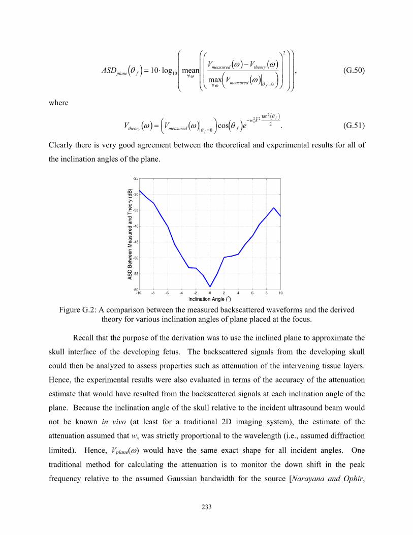
ASDV V
Vplane f
measured theory
measuredf
θω ω
ωω
ω θ
d i b g b gb g
= ⋅−
FH IK
F
HGGG
I
KJJJ
F
H
GGG
I
K
JJJ
F
H
GGG
I
K
JJJ∀
∀ =
10 10
0
2
log meanmax
, (G.50)
where
V V etheory measured f
w k
f
xf
ω ω θθ
θ
b g b g d id i
= FH IK=−
02
2 22
cos~ tan
. (G.51)
Clearly there is very good agreement between the theoretical and experimental results for all of
the inclination angles of the plane.
Figure G.2: A comparison between the measured backscattered waveforms and the derived
theory for various inclination angles of plane placed at the focus.
Recall that the purpose of the derivation was to use the inclined plane to approximate the
skull interface of the developing fetus. The backscattered signals from the developing skull
could then be analyzed to assess properties such as attenuation of the intervening tissue layers.
Hence, the experimental results were also evaluated in terms of the accuracy of the attenuation
estimate that would have resulted from the backscattered signals at each inclination angle of the
plane. Because the inclination angle of the skull relative to the incident ultrasound beam would
not be known in vivo (at least for a traditional 2D imaging system), the estimate of the
attenuation assumed that wx was strictly proportional to the wavelength (i.e., assumed diffraction
limited). Hence, Vplane(ω) would have the same exact shape for all incident angles. One
traditional method for calculating the attenuation is to monitor the down shift in the peak
frequency relative to the assumed Gaussian bandwidth for the source [Narayana and Ophir,
233
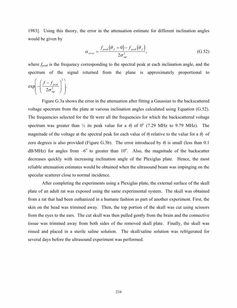
1983]. Using this theory, the error in the attenuation estimate for different inclination angles
would be given by
αθ θ
σωerror
peak f peak f
p
f f=
= −02 2
d i d i, (G.52)
where fpeak is the frequency corresponding to the spectral peak at each inclination angle, and the
spectrum of the signal returned from the plane is approximately proportional to
exp −−FHG
IKJ
FHGG
IKJJ
f f peak
p2 2
2
σω
.
Figure G.3a shows the error in the attenuation after fitting a Gaussian to the backscattered
voltage spectrum from the plate at various inclination angles calculated using Equation (G.52).
The frequencies selected for the fit were all the frequencies for which the backscattered voltage
spectrum was greater than ½ its peak value for a θf of 0o (7.29 MHz to 9.79 MHz). The
magnitude of the voltage at the spectral peak for each value of θf relative to the value for a θf of
zero degrees is also provided (Figure G.3b). The error introduced by θf is small (less than 0.1
dB/MHz) for angles from –6o to greater than 10o. Also, the magnitude of the backscatter
decreases quickly with increasing inclination angle of the Plexiglas plate. Hence, the most
reliable attenuation estimates would be obtained when the ultrasound beam was impinging on the
specular scatterer close to normal incidence.
After completing the experiments using a Plexiglas plate, the external surface of the skull
plate of an adult rat was exposed using the same experimental system. The skull was obtained
from a rat that had been euthanized in a humane fashion as part of another experiment. First, the
skin on the head was trimmed away. Then, the top portion of the skull was cut using scissors
from the eyes to the ears. The cut skull was then pulled gently from the brain and the connective
tissue was trimmed away from both sides of the removed skull plate. Finally, the skull was
rinsed and placed in a sterile saline solution. The skull/saline solution was refrigerated for
several days before the ultrasound experiment was performed.
234
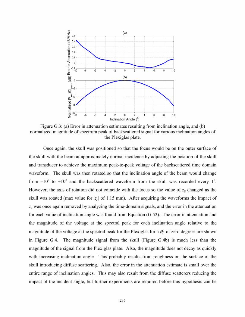
Figure G.3: (a) Error in attenuation estimates resulting from inclination angle, and (b)
normalized magnitude of spectrum peak of backscattered signal for various inclination angles of the Plexiglas plate.
Once again, the skull was positioned so that the focus would be on the outer surface of
the skull with the beam at approximately normal incidence by adjusting the position of the skull
and transducer to achieve the maximum peak-to-peak voltage of the backscattered time domain
waveform. The skull was then rotated so that the inclination angle of the beam would change
from –10o to +10o and the backscattered waveform from the skull was recorded every 1o.
However, the axis of rotation did not coincide with the focus so the value of zp changed as the
skull was rotated (max value for |zp| of 1.15 mm). After acquiring the waveforms the impact of
zp was once again removed by analyzing the time-domain signals, and the error in the attenuation
for each value of inclination angle was found from Equation (G.52). The error in attenuation and
the magnitude of the voltage at the spectral peak for each inclination angle relative to the
magnitude of the voltage at the spectral peak for the Plexiglas for a θf of zero degrees are shown
in Figure G.4. The magnitude signal from the skull (Figure G.4b) is much less than the
magnitude of the signal from the Plexiglas plate. Also, the magnitude does not decay as quickly
with increasing inclination angle. This probably results from roughness on the surface of the
skull introducing diffuse scattering. Also, the error in the attenuation estimate is small over the
entire range of inclination angles. This may also result from the diffuse scatterers reducing the
impact of the incident angle, but further experiments are required before this hypothesis can be
235
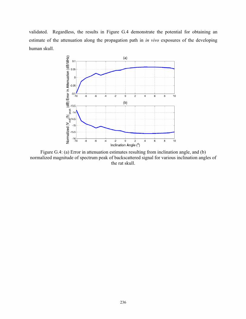
validated. Regardless, the results in Figure G.4 demonstrate the potential for obtaining an
estimate of the attenuation along the propagation path in in vivo exposures of the developing
human skull.
Figure G.4: (a) Error in attenuation estimates resulting from inclination angle, and (b)
normalized magnitude of spectrum peak of backscattered signal for various inclination angles of the rat skull.
236
VITA Timothy Allen Bigelow was born in Colorado Springs, Colorado, on December
14, 1976. He graduated from Rocky Mountain High School in Fort Collins, Colorado, in
April 1995. After high school, he enrolled in the Electrical Engineering Department at
Colorado State University (CSU) in Fort Collins. While at CSU, he received several
scholarships, including the Distinguished Scholars Award, that helped to fund his
education. He graduated summa cum laude from Colorado State University in December
1998 with a B.S. in Electrical Engineering and a minor in Mathematics. From January
1999 to May 1999, he studied religion at Faith Baptist Theological Seminary. In August
1999, he began his graduate studies in Electrical and Computer Engineering at the
University of Illinois at Urbana Champaign. The first three years of his graduate studies
were funded by the National Defense Science and Engineering Graduate Fellowship.
Initially, he studied Computer Vision under Dr. Narendra Ahuja in the computer vision
and Robotics Laboratory. Then, in January 2001, he moved to the Bioacoustics Research
Laboratory and worked under Dr. William D. O’Brien, Jr., where he completed his M.S.
thesis entitled “Experimental Evaluation on Nonlinear Indices for Ultrasound Transducer
Characterizations.” Mr. Bigelow remained in the Bioacoustics Research Laboratory until
he completed his Ph.D. thesis in April 2004. While pursuing his Ph.D. research, Mr.
Bigelow was also awarded a Beckman Institute Graduate Fellowship from September
2002 through August 2003.
243


![In vivo imaging of swimming micromotors using hybrid high … · 2020. 6. 15. · optical-ultrasound imaging technique, also called photoacoustic imaging (PAI).[28–32] PAI is](https://img.pdfslide.net/doc/110x75/6092d60f6674c8570e70cd4e/in-vivo-imaging-of-swimming-micromotors-using-hybrid-high-2020-6-15-optical-ultrasound.jpg)