Estimating the National Public Health Burden Associated ...ephtracking.cdc.gov/docs/Estimating_national_burden.pdf · Estimating the National Public Health Burden Associated ... comes

Risk Analysis DOI: 10.1111/j.1539-6924.2011.01630.x

Estimating the National Public Health Burden Associatedwith Exposure to Ambient PM2.5 and Ozone

Neal Fann,∗ Amy D. Lamson, Susan C. Anenberg, Karen Wesson, David Risley, andBryan J. Hubbell

Ground-level ozone (O3) and fine particulate matter (PM2.5) are associated with increasedrisk of mortality. We quantify the burden of modeled 2005 concentrations of O3 and PM2.5

on health in the United States. We use the photochemical Community Multiscale Air Quality(CMAQ) model in conjunction with ambient monitored data to create fused surfaces of sum-mer season average 8-hour ozone and annual mean PM2.5 levels at a 12 km grid resolutionacross the continental United States. Employing spatially resolved demographic and concen-tration data, we assess the spatial and age distribution of air-pollution-related mortality andmorbidity. For both PM2.5 and O3 we also estimate: the percentage of total deaths due to eachpollutant; the reduction in life years and life expectancy; and the deaths avoided according tohypothetical air quality improvements. Using PM2.5 and O3 mortality risk coefficients drawnfrom the long-term American Cancer Society (ACS) cohort study and National Mortality andMorbidity Air Pollution Study (NMMAPS), respectively, we estimate 130,000 PM2.5-relateddeaths and 4,700 ozone-related deaths to result from 2005 air quality levels. Among pop-ulations aged 65–99, we estimate nearly 1.1 million life years lost from PM2.5 exposure andapproximately 36,000 life years lost from ozone exposure. Among the 10 most populous coun-ties, the percentage of deaths attributable to PM2.5 and ozone ranges from 3.5% in San Jose to10% in Los Angeles. These results show that despite significant improvements in air qualityin recent decades, recent levels of PM2.5 and ozone still pose a nontrivial risk to public health.

KEY WORDS: air pollution; mortality; ozone; PM2.5; public health burden

1. INTRODUCTION

Ground-level ozone (O3) and fine particulatematter (PM2.5) are associated with increased riskof mortality.(1,2) While significant progress has beenmade in reducing ambient concentrations of air pol-lution in the United States, recent levels of O3 andPM2.5 remain elevated from the natural backgroundand are within the range of concentrations foundby epidemiology studies to affect health. This arti-cle estimates the public health burden attributable to

U.S. Environmental Protection Agency, Office of Air QualityPlanning and Standards, Research Triangle Park, NC, USA.

∗Address correspondence to Neal Fann, Mail Drop C539-07, 104T.W. Alexander Drive, Durham, NC 27711, USA; [email protected].

recent PM2.5 and ozone air quality levels within thecontinental United States.

The World Health Organization Global Burdenof Disease (GBD) study found that urban PM2.5 wasassociated with about 28,000 premature mortalitiesin the United States, Canada, and Cuba.(3,4) Anen-berg et al.(5) used a chemical transport model (reso-lution 2.8◦ × 2.8◦) to simulate O3 and PM2.5 concen-trations in both rural and urban areas, finding 35,000respiratory premature mortalities due to O3 in NorthAmerica and 141,000 cardiopulmonary and lung can-cer deaths due to PM2.5 in North America.

Using simulated rather than monitored con-centrations allows for full spatial coverage of airpollution impacts, but global chemical transport

1 0272-4332/11/0100-0001$22.00/1 C© 2011 Society for Risk Analysis

2 Fann et al.

models are generally coarsely resolved and fre-quently unable to capture fine spatial gradients ofpopulation and concentrations, particularly aroundurban areas. Global health impact assessment is alsolimited by the coarse resolution of demographic datain many locations, such as population and baselinemortality rates.

Previously, U.S. EPA calculated the publichealth burden attributable to PM2.5 in the UnitedStates at a 12 km resolution in the east and a 36 kmresolution in the west, finding that the percentage ofall-cause mortality associated with PM2.5 exposurewas as high as 11% in some counties.(6) However,that analysis did not consider O3-related or nonmor-tality impacts.

Here, we aim to quantify the burden of recentconcentrations of O3 and PM2.5 on mortality in theUnited States prior to the implementation of sev-eral recently promulgated air quality regulations thatpromise to greatly improve future air quality. Weuse the photochemical Community Multiscale AirQuality (CMAQ) model(7) in conjunction with sev-eral years of ambient monitored data to create fusedsurfaces of summer season average 8-hour ozone andannual mean PM2.5 levels at a 12 km grid resolu-tion across the continental United States. In contrastto the global analyses above, we employ finely re-solved demographic and concentration data to assessfully the spatial and age distribution of air-pollution-related mortality within specific geographic areas.We also utilize the environmental Benefits Mappingand Analysis Program (BenMAP), a software pack-age that contains a library of PM2.5 and ozone mortal-ity and morbidity concentration-response functionsand is able to automate the process of quantifyingPM2.5 and ozone health impacts from a large num-ber of scenarios. In addition, compared to previouswork this analysis expands the metrics for assessingthe public health burden for PM2.5 and ozone ex-posure by estimating the excess mortalities associ-ated with meeting hypothetical air quality improve-ments nationwide; the percentage of total mortalityattributable to these two pollutants; the estimatedlife years lost; the change in life expectancy; and theestimated PM2.5 and ozone morbidity impacts includ-ing hospitalizations and nonfatal heart attacks.

These methodological refinements enable us toanswer three key policy questions: (1) What are theestimated public health impacts of recent PM2.5 andozone levels in the United States? (2) How are theseimpacts distributed by geographic area, age, and pol-lutant? and (3) What would be the size and spatial

distribution of the health-related benefits of hypo-thetical air quality improvements?

2. METHODS

2.1. Overview of the HIA

We estimate the number of adverse health out-comes associated with population exposure to airpollution using a health impact function. The healthimpact function used in this analysis has four com-ponents: the change in air quality, the affected pop-ulation, the baseline incidence rate, and the effectestimate drawn from the epidemiological studies.(8,9)

A typical log-linear health impact function might beas follows:

�y=yo(eβ �x−1)Pop,

where y0 is the baseline incidence rate for the healthendpoint assessed; Pop is the population affected bythe change in air quality; �x is the change in air qual-ity; and β is the effect coefficient drawn from the epi-demiological study.

Here we use BenMAP (version 4.0)(10) to sys-tematize the HIA calculation process, drawing uponits library of population data, baseline incidence, andconcentration-response functions. We first describethe CMAQ air quality modeling used to simulatePM2.5 and ozone concentrations. We then detail ourselection of population estimates used to calculateexposure, baseline incidence rates used to calculaterisk, and the mortality and morbidity concentration-response functions used to assess PM2.5 and ozone-related health impacts.

2.2. PM2.5 and Ozone Air Quality Modeling

We utilize the CMAQ model(7) to estimate an-nual PM2.5 and summer season ozone concentrationsfor the year 2005 for a horizontal grid covering thecontinental United States at a 12 km resolution. TheCMAQ model is a nonproprietary computer modelthat simulates the formation and fate of photochemi-cal oxidants, including PM2.5 and ozone, for given in-put sets of meteorological conditions and emissions.The CMAQ model is a well-established and thor-oughly vetted air quality model that has seen usein a number of national and international applica-tions.(11−13) We use CMAQ version 4.71 and the U.S.

1 CMAQ version 4.7 was released on December 1, 2008. It isavailable from the Community Modeling and Analysis System(CMAS) at: http://www.cmascenter.org.

U.S. Public Health Burden of PM2.5 and Ozone 3

EPA 2005 Modeling Platform, with emissions, mete-orology, and initial and boundary conditions detailedelsewhere.(14,15) A detailed model performance eval-uation for ozone, PM2.5 and its related speciatedcomponents was conducted using observed/predictedpairs of daily/monthly/seasonal/annual concentra-tions.(14) Overall, the fractional bias, fractional error,normalized mean bias, and normalized mean errorstatistics were within the range or close to that foundin other recent applications, and determined to besufficient to provide a scientifically credible approachfor this assessment.

We improve the accuracy of the air qualitydata used in this analysis by combining the CMAQ-modeled PM2.5 and ozone concentrations with am-bient monitored PM2.5 and ozone measurements tocreate “fused” spatial surfaces for the domain shownin Figs. 1 and 2. We performed the fusion using theEPA’s Model Attainment Test Software (MATS),(16)

which employs the Voronoi neighbor averaging in-terpolation technique.(17) Fusing modeled and mea-sured ozone and PM2.5 concentrations leverages thecomplete spatial and temporal coverage of modeledconcentrations and the accuracy of observed air qual-ity measurements. This technique identifies the setof monitors that are nearest to the center of eachgrid cell, and then takes an inverse distance squaredweighted average of the monitor concentrations. Thefused spatial fields are calculated by adjusting theinterpolated ambient data (in each grid cell) up ordown by a multiplicative factor calculated as the ra-tio of the modeled concentration at the grid cell di-vided by the modeled concentration at the nearestneighbor monitor locations (weighted by distance).For PM2.5, spatial surfaces were created by fusingall 2005 valid2 modeled days of PM2.5 concentra-tions with validated PM2.5 data from 2004 to 2006from Speciated Trends Network, Interagency Mon-itoring of Protected Visual Environments, and CleanAir Status and Trends Network monitoring sites.For ozone, we only used modeling results from thesummer ozone season period between May 1 andSeptember 30, 20053 and fused these data with mon-

2 Normally, all 365 model days would have been used in the es-timation of PM2.5 levels; however during the modeling, an er-ror was discovered in the aqueous phase chemistry routines ofCMAQ v4.7. This error caused simulated hourly sulfate concen-trations to increase sporadically and in an unrealistic mannerover a very limited number of grid-cell hours over the RFS2 sim-ulations. These data were removed as described in U.S. EPA,2010b.

3 This 153-day period generally conforms to the ozone seasonacross most parts of the United States and contains the major-

itored ozone data from 2005 to 2007.4 By fusing theCMAQ-modeled air quality data with multiple yearsof ambient measured data, the air quality concentra-tions should be more reflective of a 3-year averageconcentration, and less biased by unusual changesin emissions or meteorology that may have occurredduring one year but not another (e.g., plant shutdownfor maintenance).

We calculate the total public health burden at-tributable to PM2.5 and ozone relative to “nonan-thropogenic background” concentrations of summer-season ozone and annual mean PM2.5 concentrationsthat would occur in the absence of anthropogenicemissions in the United States, Canada, and Mex-ico.(18) We identified two options to specifying thesebackground levels. The first option was to applyPM2.5 and ozone levels observed from monitors in re-mote locations. However, even remote monitors maybe affected by nonlocal sources of nonbiogenic emis-sions. Alternatively, chemical transport models allowusers to simulate background levels in the absenceof anthropogenic emissions. For ozone, we use a me-dian of the 4-hour mean value (13:00–17:00) for theeastern and western United States (22 ppb in the eastand 30 ppb in the west) reported by Fiore et al.(19)

In that analysis, the authors applied GEOS-Chem, aglobal circulation model, to model ozone formationdue to emissions originating outside of the UnitedStates.(18) We then adjusted the ozone value reportedin this study to an 8-hour maximum equivalent,(20)

consistent with the air quality metric used in theconcentration-response functions described below.

We applied background PM2.5 levels specifiedin Table 3–23 of the 2009 EPA Integrated ScienceAssessment (ISA).(18) Within the ISA, average re-gional nonanthropogenic background concentrationswere estimated using CMAQ v 4.7, with boundaryconditions from GEOS-Chem and emissions fromnatural sources everywhere in the world, and anthro-pogenic sources outside continental North Amer-ica.(18) The CMAQ modeling domain, with 36 kmgrid spacing, covered the continental United States.A model performance evaluation generally showed

ity of days with observed high ozone concentrations in 2005. Weacknowledge that the ozone season extends beyond these datesin some urban areas (e.g., Houston, L.A.) and failing to accountfor the full duration of the season in these areas may introduce adownward bias in our estimate of health impacts.

4 Normally, the calculation would have used the ambient data from2004 to 2006. However, because of the abnormally low levels ofozone measured in the continental United States in 2004 as com-pared to that measured in 2000–2007, we chose to use the ambi-ent data from the years of 2005–2007 instead.

4 Fann et al.

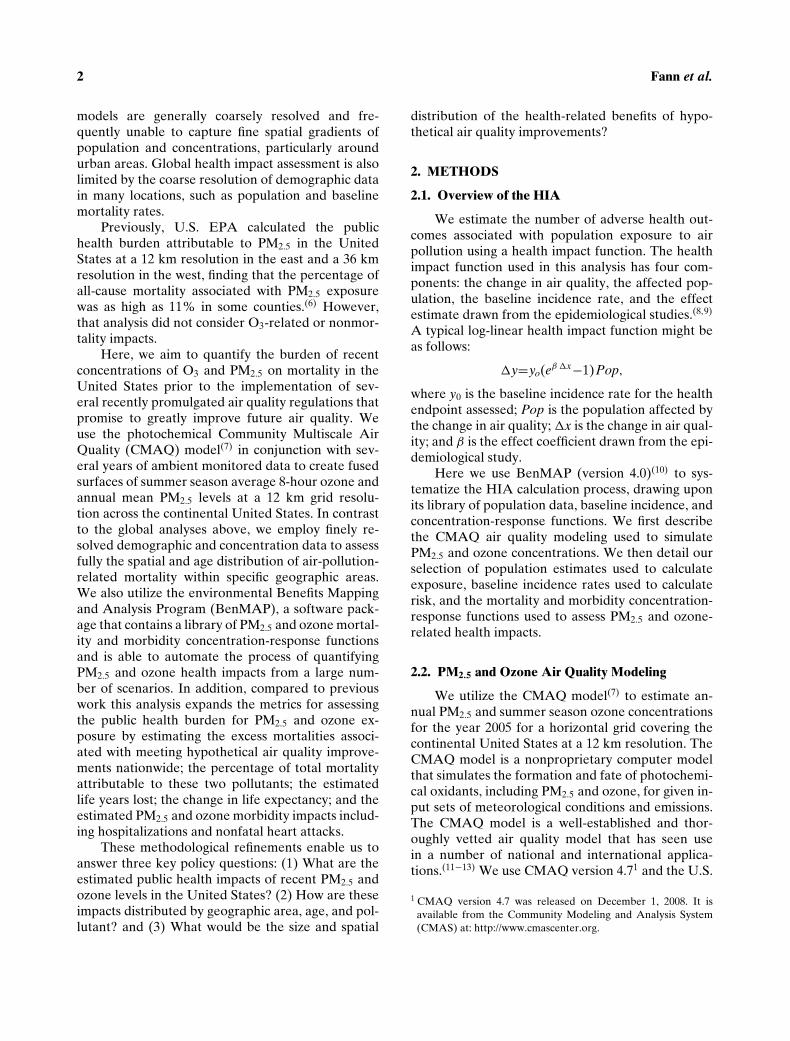
Fig. 1. Average daily 8-hour maximumsummer-season ozone levels (fusedsurface of 2005 modeled and 2004–2006monitored data).

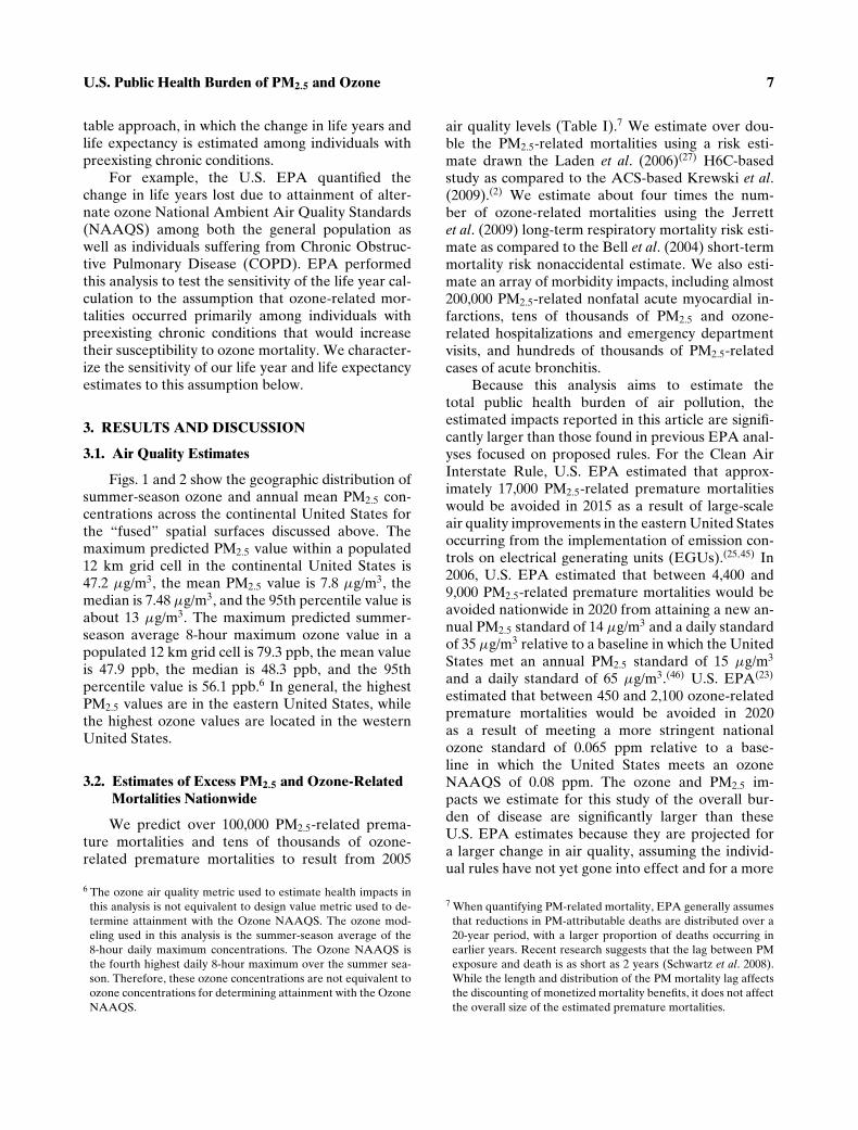
Fig. 2. Annual mean PM2.5 levels (fusedsurface of 2005 modeled and 2004–2006monitored data).

good agreement between modeled and monitoredvalues at remote sites.(18)

To determine annual regional PM2.5 backgroundconcentrations, the CMAQ domain was divided intoseven regions (i.e., Northwest, Southwest, industrialMidwest, upper Midwest, Southwest, Northwest, andsouthern California). An annual average PM2.5 con-centration was calculated for each CMAQ grid celland then a regional annual average was calculatedfrom the grid cells within each of the seven regions.These values were 0.74 μg/m3 for the Northeast,1.72 μg/m3 for the Southeast, 0.86 μg/m3 for the in-dustrial Midwest, 0.84 μg/m3 for the upper Midwest,0.62 μg/m3 for the Southwest, 1.01 μg/m3 for the

Northwest, and 0.84 μg/m3 for southern Califor-nia.(18)

2.3. Estimation of Air Quality ConcentrationsAcross the Population

We aggregate U.S. Census block-level popula-tion data(21) to the national 12 km CMAQ modelingdomain. We stratify population for the year 2000 byage, sex, race, and ethnicity categories correspond-ing to the demographic classifications considered inthe health impact functions (see later) and projectthese data to 2005 using an economic forecastingmodel.(22) Modeled PM2.5 and ozone concentrations


are matched with the population projected in each12 km grid cell and we assume that the fused air qual-ity value in each cell is the best measure of populationexposure.

2.4. Selection of Concentration-ResponseRelationships and Baseline Incidence Rates

We estimate impacts to several PM2.5-relatedhuman health endpoints, including prematuredeaths from long-term exposure, respiratory andcardiovascular-related hospital visits, asthma-relatedemergency department visits, chronic bronchitis,and nonfatal heart attacks among others. Ozone-related health endpoints include deaths from acuteand long-term exposure, respiratory hospital admis-sions, and asthma-related emergency departmentvisits among others. Table SI specifies each of theendpoints, epidemiological studies, and risk esti-mates considered in this analysis. We use annualmean PM2.5 changes as a surrogate for daily changesin PM2.5 for those functions that quantify short-term impacts; this is unlikely to add appreciablebias to the health impact estimates because theconcentration-response functions are approximatelylinear across the air quality levels experienced byU.S. populations.

We consider several factors in selecting the ap-propriate epidemiological studies and concentration-response functions for this analysis, includingwhether the study was peer reviewed, the matchbetween the pollutant studied and the pollutant ofinterest, the study design and location, and charac-teristics of the study population; this selection pro-cedure is described in detail in previous EPA regu-latory analyses.(23−25) In general, the studies utilizedhere are consistent with those applied in recent EPAregulatory analyses.(24,25) Because of the significanceof mortality as a health endpoint, we describe in de-tail the selection of the risk coefficients.

To estimate PM2.5-related long-term mortalitywe draw risk estimates from epidemiological studiesbased on data from two prospective cohort groups,often referred to as the Harvard Six-Cities Study,or “H6C,”(26,27) and the American Cancer Society“ACS” study;(2,28−30) these studies have found con-sistent relationships between fine particles and pre-mature death across multiple locations in the UnitedStates.

For PM2.5, we use from the recent Krewski et al.(2009) extended analysis of the ACS cohort the all-cause mortality risk estimate from the random effects

Cox model that controls for 44 individual and sevenecological covariates, based on average exposure lev-els for 1999–2000 over 116 U.S. cities(2) (RR = 1.06,95% confidence intervals 1.04–1.08 per 10 μg/m3 in-crease in PM2.5). We quantify all-cause mortalityrather than cardiopulmonary or lung cancer mortal-ity specifically because it is the most comprehensiveestimate of PM-related mortality. We also applied anall-cause mortality risk estimate from the Laden et al.(2006) reanalysis of the H6C cohort(27) (RR = 1.16,95% confidence intervals 1.07–1.26 per 10 μg/m3 in-crease in PM2.5).

There are strengths and weaknesses to eachPM2.5 mortality study that argue for using risk es-timates drawn from both analyses. While the ACS-based study includes a much larger population overa broader geographic area than the H6C study, theACS population is less racially diverse, better ed-ucated, and more affluent than the national aver-age. By contrast, the H6C cohort population is morerepresentative of the United States, but estimatesPM mortality risk in eastern U.S. cities where PM2.5

is generally comprised of a larger fraction of sul-fate than it is in western cities. There are other dif-ferences in population demographics and exposure-related factors that may also contribute to differencesin the eastern and western United States. To theextent that PM2.5-related mortality is strongly influ-enced by particle composition, applying a H6C-basedrisk coefficient nationwide may result in biased esti-mates of PM2.5 mortality in the west. Conversely, ap-plying an ACS-based risk estimate nationwide maynot characterize well the PM2.5 mortality impacts inthe eastern United States.(31)

While we apply both the ACS- and H6C-basedrisk coefficients, we also include in the supplement tothis article additional estimates of PM2.5-related pre-mature mortality for the western United States usingall-cause mortality risk estimates from the Krewskiet al. (2009) intra-urban analysis of the Los Ange-les region(2) (RR = 1.191, 95% confidence intervals1.06–1.33 per 10 μg/m3 increase in PM2.5) (Fig. S1).As a means of generating as comprehensive an es-timate of mortality possible, to also quantify PM-related infant deaths using a risk estimate from thecohort study by Woodruff et al.(32) This study founda significant link between PM10 and infant death be-tween 2 and 12 months of age. (RR = 1.04, 95% con-fidence intervals 1.02–1.07 per 10 μg/m3 increase inPM2.5).

For ozone, we estimate the change in ozone-related premature mortality applying both short- and

6 Fann et al.

long-term risk estimates. A number of time-seriesozone mortality studies including an analysis byHuang et al. (2004) in Los Angeles(33) and an anal-ysis by Schwartz (2005)(34) in Houston have strength-ened the findings of previous studies finding a re-lationship between short-term ozone exposure andpremature mortality. The Bell et al. (2004)(1) anal-ysis of the National Morbidity, Mortality, and AirPollution Study (NMMAPS) data set and the meta-analyses by Bell et al. (2005),(35) Ito et al. (2005),(36)

and Levy et al. (2005)(37) sought to resolve the re-lationship between ozone, PM, weather-related vari-ables, seasonality, and other variables. We apply theBell et al. (2004) ozone nonaccidental mortality rela-tive risk estimate (RR = 1.0052, 95% confidence in-tervals 1.0027–1.0077 per 10 ppb ozone increase)(1)

because it is broadly cited. This study is also anNMMAPS-based analysis, which applies a commonmethodology to all cities, suggesting that it is notsubject to the same risk of publication bias as themeta-analyses, which include the results of single-citystudies.5(38)

Recent evidence also suggests a relationship be-tween long-term exposure to ozone and prematurerespiratory mortality in the ACS cohort (Jerrettet al. 2009).(39) Jerrett et al. find that long-termexposure to ozone is associated with respiratorypremature mortality in a two-pollutant model thatcontrols for PM2.5. The Jerrett et al. (2009) estimaterepresents one of the few studies detecting an in-crease in mortality risk from long-term exposure toozone. From this study, we apply a long-term respira-tory mortality estimate (RR = 1.040, 95% confidenceintervals 1.013–1.067 per 10 ppb ozone increase) as ameans of capturing the impact of long-term ozone ex-posure. Until the literature evolves further, it will re-main unclear whether the biological mechanisms un-derlying the ozone-related deaths detected by theseshort- and long-term studies are similar or different.By extension, the literature may also resolve the de-gree to which these studies are each detecting thesame mortalities, over different periods of time. Thisuncertainty has implications for our findings, whichwe discuss below.

5 Anderson and colleagues cite three reasons that single-city stud-ies may be more prone to publication bias: (1) such studies fre-quently rely on easily available daily mortality counts, and re-searchers may be less inclined to publish negative findings; (2)the statistical modeling for time series entail a level of subjectiv-ity and (3) each study can produce a large number of estimatesand the researchers may select estimates based on the directionof their effect.

Because epidemiological studies assess changesin risk relative to some baseline rate, we use abaseline incidence rate for each health endpointin the analysis (Table SII). Ideally, the incidencerate should also be matched to the geographicarea of focus so that it describes the health sta-tus of the population of interest. In this analysiswe apply a three-year average of 2006–2008 cause-specific county-level mortality rates from the CDC-WONDER database as a surrogate for 2005 mortal-ity rates.(40) Morbidity rates are either national orregional averages depending on the data source(Table SII).

2.5. Calculating Health Impacts

Quantifying the number of PM2.5 and ozone-related excess mortalities and morbidities involvedspecifying the health impact function with each ofthe key data inputs described above. This calcula-tion produces counts of mortality and morbidity im-pacts. We estimate 95% confidence intervals aroundeach mean health impact estimate using the MonteCarlo method, which samples a distribution basedon the standard error reported in each epidemiolog-ical study. All estimated PM-related deaths are at-tributed to exposures to 2005 air quality, which weassume to occur over a 20-year period following thisexposure, though recent research suggests that thelag between PM exposure and death is as short as2 years.(25,41) We calculate the percentage of prema-ture PM2.5 and ozone-related mortality by dividingthe number of excess deaths by the total number ofcause-specific deaths in each county.

One criticism of the excess- or attributable-mortality calculation is that readers may infer thatreductions in air pollution exposure result in deathsavoided altogether, when in fact these deaths are sim-ply deferred into the future.(42) For this reason, weuse standard life tables available from the Centersfor Disease Control,(43) we estimate the number oflife years and life expectancy lost to air pollution. Wecalculate the number of life years lost using the fol-lowing formula:

Total Life Years =n∑

i=1

LEi × Mi ,

where LEi is the remaining life expectancy for age in-terval i, Mi is the change in number of deaths in ageinterval i, and n is the number of age intervals.(44) Al-ternate analyses have employed a cause-modified life


table approach, in which the change in life years andlife expectancy is estimated among individuals withpreexisting chronic conditions.

For example, the U.S. EPA quantified thechange in life years lost due to attainment of alter-nate ozone National Ambient Air Quality Standards(NAAQS) among both the general population aswell as individuals suffering from Chronic Obstruc-tive Pulmonary Disease (COPD). EPA performedthis analysis to test the sensitivity of the life year cal-culation to the assumption that ozone-related mor-talities occurred primarily among individuals withpreexisting chronic conditions that would increasetheir susceptibility to ozone mortality. We character-ize the sensitivity of our life year and life expectancyestimates to this assumption below.

3. RESULTS AND DISCUSSION

3.1. Air Quality Estimates

Figs. 1 and 2 show the geographic distribution ofsummer-season ozone and annual mean PM2.5 con-centrations across the continental United States forthe “fused” spatial surfaces discussed above. Themaximum predicted PM2.5 value within a populated12 km grid cell in the continental United States is47.2 μg/m3, the mean PM2.5 value is 7.8 μg/m3, themedian is 7.48 μg/m3, and the 95th percentile value isabout 13 μg/m3. The maximum predicted summer-season average 8-hour maximum ozone value in apopulated 12 km grid cell is 79.3 ppb, the mean valueis 47.9 ppb, the median is 48.3 ppb, and the 95thpercentile value is 56.1 ppb.6 In general, the highestPM2.5 values are in the eastern United States, whilethe highest ozone values are located in the westernUnited States.

3.2. Estimates of Excess PM2.5 and Ozone-RelatedMortalities Nationwide

We predict over 100,000 PM2.5-related prema-ture mortalities and tens of thousands of ozone-related premature mortalities to result from 2005

6 The ozone air quality metric used to estimate health impacts inthis analysis is not equivalent to design value metric used to de-termine attainment with the Ozone NAAQS. The ozone mod-eling used in this analysis is the summer-season average of the8-hour daily maximum concentrations. The Ozone NAAQS isthe fourth highest daily 8-hour maximum over the summer sea-son. Therefore, these ozone concentrations are not equivalent toozone concentrations for determining attainment with the OzoneNAAQS.

air quality levels (Table I).7 We estimate over dou-ble the PM2.5-related mortalities using a risk esti-mate drawn the Laden et al. (2006)(27) H6C-basedstudy as compared to the ACS-based Krewski et al.(2009).(2) We estimate about four times the num-ber of ozone-related mortalities using the Jerrettet al. (2009) long-term respiratory mortality risk esti-mate as compared to the Bell et al. (2004) short-termmortality risk nonaccidental estimate. We also esti-mate an array of morbidity impacts, including almost200,000 PM2.5-related nonfatal acute myocardial in-farctions, tens of thousands of PM2.5 and ozone-related hospitalizations and emergency departmentvisits, and hundreds of thousands of PM2.5-relatedcases of acute bronchitis.

Because this analysis aims to estimate thetotal public health burden of air pollution, theestimated impacts reported in this article are signifi-cantly larger than those found in previous EPA anal-yses focused on proposed rules. For the Clean AirInterstate Rule, U.S. EPA estimated that approx-imately 17,000 PM2.5-related premature mortalitieswould be avoided in 2015 as a result of large-scaleair quality improvements in the eastern United Statesoccurring from the implementation of emission con-trols on electrical generating units (EGUs).(25,45) In2006, U.S. EPA estimated that between 4,400 and9,000 PM2.5-related premature mortalities would beavoided nationwide in 2020 from attaining a new an-nual PM2.5 standard of 14 μg/m3 and a daily standardof 35 μg/m3 relative to a baseline in which the UnitedStates met an annual PM2.5 standard of 15 μg/m3

and a daily standard of 65 μg/m3.(46) U.S. EPA(23)

estimated that between 450 and 2,100 ozone-relatedpremature mortalities would be avoided in 2020as a result of meeting a more stringent nationalozone standard of 0.065 ppm relative to a base-line in which the United States meets an ozoneNAAQS of 0.08 ppm. The ozone and PM2.5 im-pacts we estimate for this study of the overall bur-den of disease are significantly larger than theseU.S. EPA estimates because they are projected fora larger change in air quality, assuming the individ-ual rules have not yet gone into effect and for a more

7 When quantifying PM-related mortality, EPA generally assumesthat reductions in PM-attributable deaths are distributed over a20-year period, with a larger proportion of deaths occurring inearlier years. Recent research suggests that the lag between PMexposure and death is as short as 2 years (Schwartz et al. 2008).While the length and distribution of the PM mortality lag affectsthe discounting of monetized mortality benefits, it does not affectthe overall size of the estimated premature mortalities.

8 Fann et al.

Table I. Estimated PM2.5 and Ozone-Related Health ImpactsDue to 2005 Modeled Air Quality (Relative to Nonanthropogenic

Background).

Annual Impact EstimatesHealth Effect (95% Confidence Interval)a

PM-related endpointsPremature mortality

Krewski et al. (2009) (age >29) 130,000(51,000–200,000)

Laden et al. (2006) (age >24) 320,000(180,000–440,000)

Infant (< 1 year) 1,800(−1,500–4,800)

Chronic bronchitis (age > 27) 83,000(16,000–140,000)

Nonfatal heart attacks (age > 17) 180,000(70,000–270,000)

Hospital admissions— 30,000respiratory (all ages) (15,000–45,000)

Hospital admissions— 62,000cardiovascular (age > 18) (44,000–73,000)

Emergency room visits 110,000for asthma (age < 18) (68,000–150,000)

Acute bronchitis (ages 8–12) 200,000(−7,600–350,000)

Lower respiratory 2,400,000symptoms (ages 7–14) (1,200,000–3,500,000)

Upper respiratory symptoms 2,000,000(asthmatics age 9–18) (640,000–3,400,000)

Asthma exacerbation 2,500,000(asthmatics 6–18) (280,000–6,800,000)

Lost work days (ages 18–65) 18,000,000(15,000,000–20,000,000)

Minor restricted-activity 100,000,000days (ages 18–65) (87,000,000–120,000,000)

Ozone-related endpointsPremature mortality

Bell et al. (2004) (all ages) 4,700(1,800–7,500)

Jerrett et al. (2009) (age >29) 19,000(7,600–29,000)

Hospital admissions— 31,000respiratory causes (age > 64) (1,200–53,000)

Hospital admissions— 27,000respiratory causes (age <2) (13,000–39,000)

Emergency room visits 19,000for asthma (all ages) (−1,200–58,000)

Minor restricted-activity 29,000,000days (ages 18–65) (14,000,000–44,000,000)

School absence days 11,000,000(4,500,000–16,000,000)

a95% confidence intervals calculated using a Monte Carlo methodbased on the standard error reported in each epidemiologicalstudy. Health impacts attributable to 2005 air quality levels. Weassume a time lag between initial exposure to PM2.5 and death.

comprehensive cross-section of U.S. population. Ta-ble SIII summarizes the per-person reduction inPM2.5 exposure between 2005 and 2014, when a re-

cently proposed rule expected to achieve significantemission reductions from EGUs is scheduled to takeeffect.

3.3. Detailed Estimates of Impacts by Region, Age,and Air Quality Level

While the total estimates of excess mortality andmorbidity help characterize the overall national pub-lic health burden attributable to recent air quality,they provide limited insight into how these estimatedimpacts are distributed by geographic location or byage. Below we: (1) consider the spatial distributionof these estimated mortality impacts; (2) characterizethe PM2.5 and ozone-related impacts according to thenumber of life years lost, change in life expectancy,and the percentage of total mortality attributable tothese pollutants; and (3) quantify the reduction inmortality impacts according to hypothetical improve-ments in air quality. Unless otherwise noted, each ofthese analyses apply PM2.5 and ozone mortality riskcoefficients from the Krewski et al. and Bell et al.studies, respectively.(1,2)

3.3.1. The Spatial Distribution of PM2.5

and Ozone-Related Excess Mortalities

To illustrate the spatial distribution of the pub-lic health burden, we provide maps of the combinedPM2.5 and ozone-related mortality impacts by countyin Fig. 3. These maps also identify the seven geo-graphic regions previously used by the U.S. EPAwhen performing air quality and health impact analy-ses.(6) In any given location the number of the PM2.5-related mortalities will be influenced by the combina-tion of air quality, population density, and baselinehealth status. On a per-person basis, southern Cal-ifornia and the industrial Midwest see the greatestexposure to PM2.5. However, the confluence of poorair quality, population size and density, and base-line health status cause the largest number of esti-mated PM2.5-related excess premature mortalities tooccur within the Northeast, Southeast, and Midwest-ern United States. Among urban areas, the largestestimated impacts occur in L.A., Chicago, Detroit,Pittsburgh, Houston, New York, Philadelphia, andBoston. The estimated ozone-related mortality im-pacts are an order of magnitude smaller than thoseestimated for PM2.5, partly due to the smaller rel-ative risk associated with ozone, and generally dis-tributed among the same counties affected most byPM2.5 mortality.


Fig. 3. PM2.5 and ozone-related excess mortalities at the county level by geographic area.

Fig. 4. The number of ozone-relatedexcess mortalities avoided by air qualitybenchmark and region of the UnitedStates (using Jerrett et al. 2009 riskestimate).

We also consider how the estimated number ofavoided PM2.5 and ozone deaths changes if we as-sume that air quality incrementally improves (Figs. 4and 5). For example, we estimate that about 23,000PM2.5-related mortalities would be avoided as a re-sult of lowering 2005 annual mean PM2.5 levels downto 10 μg/m3 nationwide. We estimate about 80,000premature mortalities would be avoided by lower-ing PM2.5 levels to 5 μg/m3 nationwide. We haveless confidence in impacts estimated below the low-est measured level of the PM2.5 mortality studiesbecause we are less certain of the shape of theconcentration-response relationship at these levels.However, given that there is little evidence for a

threshold PM2.5 mortality function, such estimatesstill give some insight into the fraction of the publichealth benefits of air quality improvements at lowerPM2.5 levels. The avoided PM2.5 and ozone-relatedmortalities appear to increase in an approximatelylinear fashion as we reduce air quality levels to lowerbenchmarks. The reduction in O3 and PM2.5-relatedexcess mortalities are not distributed evenly acrossthe United States, and most are concentrated in theNortheast, Southeast, and industrial Midwest.8

8 The ozone air quality benchmarks represent various daily 8-hourmaximum levels averaged over the summer season and equiv-alent with ozone NAAQS levels, which are set according to a

10 Fann et al.

Fig. 5. The number of PM2.5-relatedexcess deaths avoided by air qualitybenchmark and region of the UnitedStates (using Krewski et al. 2009 riskestimate).

Fig. 6. Percentage of premature deathsattributable to 2005 PM2.5 and ozone airquality by U.S. county.

3.3.2. Estimating the Percentage of All DeathsAttributable to PM2.5 and Ozone and theChange in Life Years and Life Expectancy

The counties with the largest estimated percent-age of mortality due to PM2.5 and ozone tend to be inthe northeastern United States, the industrial Mid-west, and southern California (Fig. 6). The cumula-tive distribution of the percentage of mortality at-tributable to PM2.5 and ozone indicates that amongthe most populous counties, the proportion of totaldeaths attributable to PM2.5 and ozone ranges from

fourth highest daily design value. As such, health impacts at eachozone benchmark level do not reflect the health benefits of meet-ing different NAAQS levels.

a low of 3.5% in San Jose to as high as 10% in LosAngeles (Fig. 7). Nationwide, the percentage rangesfrom less than 1% to about 10% in southern Califor-nia. We also estimate that about 19% of all ischemic-heart-disease-related deaths are attributable to PM2.5

nationwide (Table SIV).The overall percentage of all deaths due to PM2.5

is much higher than it is for ozone (Figs. S2 andS3). While the percentage of all deaths attributableto PM2.5 exposure is significantly higher in south-ern California than other regions, the percentageof total mortality from ozone exposure is roughlyequal for southern California, the industrial Midwest,and to a lesser extent the Northeast and Southeast,and significantly lower in the Pacific Northwest. The


Fig. 7. The cumulative distribution of thepercentage of all-cause mortalityattributable to PM2.5 and ozone amongthe 10 most populous U. S. counties.

spatial distribution of this metric and modeled ozonelevels are fairly consistent across the United States.For both ozone and PM2.5, the percentage appearsto decline modestly for older populations, suggestingthat older populations may live in areas with lowermodeled concentrations.

We estimate a large number of life years lostto PM2.5 and ozone and this number varies by re-gion of the country and by age (Figs. S4 and S5).For both PM2.5 and ozone, the Northeast, Southeast,and industrial Midwest show the largest estimated to-tal number of life years lost. Because the estimate oflife years lost is influenced in part by the total num-ber of individuals affected, we also estimate the per-centage of these PM2.5 and ozone-related life yearslost by age range and region, which controls for dif-ferences in the size of the populations within eachregion (Table SV). Among populations aged 65–99,we estimate nearly 1.1 million life years lost fromPM2.5 exposure and approximately 36,000 life yearslost from ozone exposure. The statistical abstract ofthe U.S. Census(47) reported 15 million life years lostamong populations aged 65–99 from all causes in2005, implying that PM2.5 and ozone-related mortal-ity accounted for approximately 7% of total life yearslost among populations ages 65–99 nationwide in2005.

Finally, using a standard life table, we quan-tify the change in life expectancy at birth and by 5-year age increment resulting from the elimination ofPM2.5 and ozone-related mortality risk (Table SVI).Among populations at birth, we estimate a change

in life expectancy of 0.7 years, a result that comportswell with recent analyses of the effect of air pollutionon life expectancy.(48)

When calculating changes in life expectancy, weassume that the life expectancy of those dying fromair pollution is the same as the general population.It is possible to characterize the sensitivity of this as-sumption by referring to a 2008 U.S. EPA analysis oflife years lost due to ozone exposure.(44) That analy-sis estimated approximately 14–53% fewer life yearslost when assuming that populations dying prema-ture from ozone exposure suffered average-to-severeCOPD, as compared to the assumption that thesepopulations shared the same life expectancy as thegeneral population.

However, using a standard life table is reason-able when considering that: (1) the vast majority ofpremature deaths are estimated to occur among pop-ulations aged >64, half of whom suffer from oneor more chronic illnesses, suggesting that a stan-dard life table captures the change in life expectancyamong a substantial number of individuals whosuffer such chronic illnesses; and (2) a recent long-term study found that PM2.5 initiated cardiovascu-lar events among women with no history of car-diovascular disease—underscoring the role of airpollution in both promoting chronic illness and caus-ing premature death.(49−51) Moreover, recent evi-dence available since the publication of that EPA re-port suggests that ozone-induced deaths do not occurexclusively, or even mostly, among individuals withsuch preexisting conditions.(52,53)

12 Fann et al.

4. DISCUSSION AND CONCLUSIONS

We have estimated the recent burden of PM2.5

and ozone on human health in the United States,using ambient measurements, 2005 and nonan-thropogenic background PM2.5 and O3 concentra-tions simulated by atmospheric chemistry models,and a health impact function. We find that be-tween 130,000 and 340,000 premature deaths are at-tributable to PM2.5 and O3. We also find that ge-ographic and age distribution of this health risk isnot shared equally. Major metropolitan areas in-cluding L.A., Houston, Pittsburgh, and New Yorksee the largest number of estimated excess PM2.5

and ozone-related deaths. Southern California is es-timated to experience the largest percentage of to-tal mortality attributable to PM2.5 across all ages(between 7% and 17% depending on the risk esti-mate used), while the greatest percentage of mor-tality attributable to ozone is the highest in theindustrial Midwest (between 0.24% and 1%, againdepending on the risk estimate used). Conversely,the largest estimated number of PM2.5 and ozone-related life years lost are in the Southeast. Whileestimating the contribution of air pollution to totalmorbidity impacts is difficult due to incomplete dataon hospitalizations and other health endpoints, wefind that the nonmortality impacts of air pollution aresubstantial, consistent with previous studies estimat-ing air pollution mortality and morbidity.(3,4)

The size of these mortality estimates is com-parable to those reported in Anenberg et al.(5) forNorth America and larger than those reported byCohen et al.(3,4) Although our estimates may belarger than those of Cohen et al.,(3,4) our analysis in-cludes several factors that may explain these differ-ences. In particular, we estimate impacts relative tonatural background and utilize modeled air qualitythat better represents population exposures in ruraland urban areas. This general consistency with priorestimates of PM2.5 and ozone impacts reaffirms thatdespite significant improvements in air quality in re-cent decades, recent levels of ozone and PM2.5 stillpose a public health risk in many regions of theUnited States. PM2.5 and ozone impose a nontriv-ial level of mortality risk, particularly when com-pared to other causes of death. For example, whilethis analysis estimates between 130,000 and 340,000PM2.5 and ozone-attributable deaths from 2005 airquality, in this same year there were approximately120,000 deaths due to accidents, 72,000 deaths due toAlzheimer’s, and 63,000 deaths due to influenza.(54)

It is more challenging to evaluate the contribu-tion of air pollution to total morbidity impacts. Forexample, incomplete information regarding the to-tal number and spatial distribution of asthma hospi-talizations prevent us from calculating the percent-age of total asthma hospitalizations attributable toPM2.5 with confidence. However, analyses includingthe GBD(3,4) provide evidence that the nonmortalityimpacts of air pollution are substantial—a finding re-inforced by these results.

The estimates presented here are subject to anumber of important limitations and uncertainties,only some of which we can quantify. Many of theseare endemic to health impact assessments (e.g., thetransfer of risk estimates from epidemiology studiesto other contexts and the selection of epidemiologicalstudies used to quantify impacts) and are describedin detail elsewhere.(25,55) However, certain sourcesof uncertainties are likely to influence the analysisgreatly and are worth noting here. This health im-pact analysis relies upon modeled air quality esti-mates that utilize a national emissions inventory. Pre-vious analyses(46) have found that even small errorsin emission inventory, when compounded with otheruncertainties in the analysis, can have a significantimpact on the overall size of the estimated healthimpacts.

Alternative methods for assessing air pollutionhealth impacts might also have yielded different re-sults. As noted earlier, the estimated life years lostand changes in life expectancy are sensitive to theassumption that populations dying prematurely fromair pollution exposure share the same life expectancyas the general population. Assuming that air pol-lution deaths occur only among populations withpreexisting chronic conditions yields significantlydifferent results—though the empirical evidence sug-gests that premature death does not occur exclusivelyamong such populations.(53) As another example ofhow alternative methods would have affected our re-sults, we might have employed an Institute of Occu-pational Medicine (IOM)-style life table approach,calculating lifetime air pollution risk among a cohortof individuals. A principal advantage of this tech-nique is that it characterizes changes in risk among apopulation cohort over time and reduces the chancethat the same health impact may be counted twicefrom one year to the next.

Due in part to the limited availability of air qual-ity modeling estimates, this analysis estimated healthimpacts and life expectancy changes attributable toair pollution exposure in a single historical year.


Future research might build upon this analysis byemploying the IOM life-table tool in conjunctionwith both historical and projected air quality. Sucha method would yield an improved characterizationof the public health burden over time after the im-plementation of national air quality regulations.

Another approach is the comparative risk anal-ysis method applied by the GBD, which aims toestimate air-pollution-related impacts within a riskframework that evaluates air pollution health im-pacts as one among many sources of public healthrisks.(3,4) One advantage of this type of compara-tive risk assessment is that by attempting to system-atically account for all sources of mortality risk, ofwhich air pollution is one component, it may reducethe potential for attributing an incorrect fraction oftotal mortality risk to air pollution. The GBD ap-proach also aims to apportion air pollution risk ac-cording to indoor and outdoor exposure, which datalimitations prevented this analysis from attempting.

Estimating PM2.5 mortality and long-term ozonemortality impacts down to nonanthropogenic back-ground levels also introduces important uncertain-ties. A sizable proportion of the total mortality at-tributed to these two pollutants occurs at air qualitylevels below the lowest measured level of each study(Figs. 4 and 5). Estimates of mortality impacts at airquality levels below the observable data in the epi-demiology study are inherently more uncertain be-cause at these levels we have less confidence in theshape of the concentration-response curve, althoughthere is little evidence to suggest there is a thresholdin the concentration-response functions.

We based PM2.5 and ozone mortality and mor-bidity estimates on recent air quality concentrations.As such, our results do not reflect the importantair quality improvements expected to result froman array of U.S. EPA and state air quality man-agement programs that will be implemented in thenear future—including the nonroad diesel rule, Tier-2 vehicle standards, the proposed transport rule, anda several maximum achievable control technologystandards, among other rules. U.S. EPA projectionsof future air quality indicate that overall ambient lev-els of PM2.5 and ozone will decline significantly com-pared to those levels estimated here. We anticipatethat these rules will address a large portion of thePM2.5 and O3 public health burden identified in thisarticle.

Another key uncertainty is the use of both time-series and cohort studies to quantify mortality im-pacts and changes in life years and life expectancy.

While we estimate PM2.5-related mortality using riskestimates drawn from two long-term cohort studies,we use both a short-term time-series study and along-term cohort study to quantify ozone impacts.PM2.5 cohort analyses are generally understood tobetter characterize the total risk of PM2.5 exposureover time because they capture the impacts of bothlong-term and some portion of short-term expo-sures.(46,53,56) However, it is less clear as to whetherthere is a separate short- and long-term mortality im-pact related to ozone exposure—or whether the long-term study used in this analysis might be capturingthese impacts. For this reason, there is some uncer-tainty as to whether the ozone mortality impacts es-timated using the Levy et al. (2005) short-term studyand the Jerrett et al. (2009) long-term study are addi-tive or overlapping.

ACKNOWLEDGMENTS

We greatly appreciate the contributions ofAaron Cohen in helping shape the conceptual basisfor this article.

REFERENCES

1. Bell ML, McDermott A, Zeger SL, Samet J, Dominici, F.Ozone and short-term mortality in 95 US urban communi-ties, 1987–2000. Journal of the American Medical Associa-tion, 2004; 292(19):2372–2378.

2. Krewski D, Jerrett M, Burnett RT, Ma R, Hughes E, Shi Y,Turner C, Pope CA, Thurston G, Calle EE, Thunt MJ. Ex-tended follow-up and spatial analysis of the American CancerSociety study linking particulate air pollution and mortality.HEI Research Report, 140. Boston, MA: Health Effects In-stitute, 2009.

3. Cohen AJ, Anderson HR, Ostro B, Pandey KD,Krzyzanowski M, Kuenzli N, Gutschmidt K, Pope CA,Romieu I, Samet JM, Smith KR. Mortality impacts of urbanair pollution. In Ezzati M, Lopez AD, Rodgers A, MurrayCUJL (eds). Comparative Quantification of Health Risks:Global and Regional Burden of Disease Due to Selected Ma-jor Risk Factors, Vol. 2. Geneva: World Health Organization,2004.

4. Cohen AJ, Anderson HR, Ostro B, Pandey KD,Krzyzanowski M, Kuenzli N, Gutschmidt K, Pope CA,Romieu I, Samet JM, Smith KR. The global burden ofdisease due to outdoor air pollution. Journal of Toxicologyand Environmental Health, 2005; 68(13):1301–1307.

5. Anenberg SC, Horowitz LW, Tong DQ, West JJ. An estimateof the global burden of anthropogenic ozone and fine par-ticulate matter on premature human mortality using atmo-spheric modeling. Environmental Health Perspectives, 2010;118:1189–1195.

6. U.S. Environmental Protection Agency (U.S. EPA). Quan-titative Health Risk Assessment for Particulate Matter. Re-search Triangle Park, NC: Office of Air Quality Planning andStandards, 2010. Available at: http://www.epa.gov/ttn/naaqs/standards/pm/data/20100209RA2ndExternalReviewDraft.pdf.Accessed April 25, 2011.

14 Fann et al.

7. Byun DW, Schere KL. Review of the governing equa-tions, computational algorithms, and other components of theModels-3 Community Multiscale Air Quality (CMAQ) mod-eling system. Applied Mechanics Reviews, 2006; 59(2):51–77.

8. Hubbell BJ, Hallberg A, McCubbin D, Post, E. Health-related benefits of attaining the 8-hr ozone standard. Envi-ronmental Health Perspectives, 2006; 113:73–82.

9. Hubbell BJ, Fann N, Levy JI. Methodological considerationsin developing local-scale health impact assessments: Balanc-ing national, regional and local data. Air Quality Atmosphereand Health, 2009; 2:99–110.

10. Abt Associates, Inc. Environmental Benefits and MappingProgram (Version 4.0), 2010. Bethesda, MD. Prepared forU.S. Environmental Protection Agency Office of Air QualityPlanning and Standards. Research Triangle Park, NC. Avail-able at: http://www.epa.gov/air/benmap. Accessed April 25,2011.

11. Hogrefe C, Biswas J, Lynn B, Civerolo K., Ku JY, Rosen-thal J, Rosenzweig C, Goldberg R, Kinney PL. Simulatingregional-scale ozone climatology over the eastern UnitedStates: Model evaluation results. Atmospheric Environment,2004; 38(17):2627–2638.

12. U.S. Environmental Protection Agency (U.S. EPA). Tech-nical Support Document for the Final Locomotive/MarineRule: Air Quality Modeling Analyses, 2008. Research Trian-gle Park, NC: U.S. Environmental Protection Agency, Officeof Air Quality Planning and Standards, Air Quality Assess-ment Division.

13. Lin M, Oki T, Holloway T, Streets DG, Bengtsson M, KanaeS. Long-range transport of acidifying substances in East Asia-Part I: Model evaluation and sensitivity studies. AtmosphericEnvironment, 2008; 42(24):5939–5955.

14. U.S. Environmental Protection Agency (U.S. EPA). AirQuality Modeling Technical Support Document: Changesto the Renewable Fuel Standard Program, 2010. Office ofAir Quality Planning and Standards, Research Triangle Park,NC. EPA 454/R-10–001. Available at: http://www.epa.gov/otaq/renewablefuels/454r10001.pdf. Accessed April 25,2011.

15. U.S. Environmental Protection Agency (U.S. EPA). RFS2Emissions Inventory for Air Quality Modeling TechnicalSupport Document, 2010. Office of Air Quality Planningand Standards, Research Triangle Park, NC. EPA-420-R-10–005. Available at: http://www.epa.gov/otaq/renewablefuels/420r10005.pdf. Accessed April 25, 2011.

16. Abt Associates, Inc. Model Attainment Test Software(Version 2), 2010. Bethesda, MD. Prepared for U.S. Envi-ronmental Protection Agency Office of Air Quality Planningand Standards. Research Triangle Park, NC. Availableat: http://www.epa.gov/scram001/modelingapps˙mats.htm.Accessed April 25, 2011.

17. Timin B, Wesson K, Thurman J. Application of Model andAmbient Data Fusion Techniques to Predict Current and Fu-ture year PM2.5 concentration in unmonitored areas. Pp. 175–179 in Steyn DG, Rao St (eds). Air Pollution Modeling andIts Application XX. Netherlands: Springer, 2010.

18. U.S. Environmental Protection Agency (U.S. EPA). In-tegrated Science Assessment for Particulate Matter (Fi-nal Report), 2009. EPA-600-R-08–139F. National Centerfor Environmental Assessment—RTP Division. Availableat: http://cfpub.epa.gov/ncea/cfm/recordisplay.cfm?deid=216546. Accessed April 25, 2011.

19. Fiore AM, Jacob DJ, Bey I, Yantosca RM, Field BD, FuscoAC, Wilkinson JG. Background ozone over the United Statesin summer—Origin, trend, and contribution to pollutionepisodes. Journal of Geophysical Research. D. Atmospheres,2002; 107(D15):ACH 11–1 to ACH 11–25.

20. Anderson BG, Bell ML. Does one size fit all? The suitabilityof standard ozone exposure metric conversion ratios and im-

plications for epidemiology. Journal of Exposure Science andEnvironmental Epidemiology, 2010; 20:2–11

21. GeoLytics Inc. 2001. CensusCD R© 1990 + Maps, Release 4.1.CD-ROM. GeoLytics, Inc.

22. Woods & Poole Economics Inc. 2008. Population by SingleYear of Age CD. CD-ROM. Woods & Poole Economics, Inc.Washington, D.C.

23. U.S. Environmental Protection Agency (U.S. EPA). Regu-latory Impact Analysis, 2008 National Ambient Air QualityStandards for Ground-Level Ozone, Chapter 6, 2008. Officeof Air Quality Planning and Standards, Research TrianglePark, NC. Available at http://www.epa.gov/ttn/ecas/regdata/RIAs/6-ozoneriachapter6.pdf. Accessed April 25, 2011.

24. U.S. Environmental Protection Agency (U.S. EPA). FinalRegulatory Impact Analysis (RIA) for the NO2 NationalAmbient Air Quality Standards (NAAQS), 2010. Officeof Air Quality Planning and Standards, Research Tri-angle Park, NC. Available at http://www.epa.gov/ttn/ecas/regdata/RIAs/FinalNO2RIAfulldocument.pdf. AccessedApril 25, 2011.

25. U.S. Environmental Protection Agency (U.S. EPA). Reg-ulatory Impact Analysis for the Final Clean Air Inter-state Rule, 2005. Office of Air and Radiation. Available athttp://www.epa.gov/cair/pdfs/finaltech08.pdf. Accessed April25, 2011.

26. Dockery DW, Pope CA, Xu XP, Spengler JD, Ware JH, FayME, Ferris BG, Speizer FE. An association between air pol-lution and mortality in six U.S. cities. New England Journalof Medicine, 1993; 329(24):1753–1759.

27. Laden F, Schwartz J, Speizer FE, Dockery DW. Reduction infine particulate air pollution and mortality. American Journalof Respiratory and Critical Care Medicine, 2006; 173:667–672.

28. Pope CA, Thun MJ, Namboodiri MM, Dockery DW, EvansJS, Speizer FE, Heath CW. Particulate air pollution as apredictor of mortality in a prospective study of U.S. adults.American Journal of Respiratory Critical Care Medicine,1995; 151:669–674.

29. Pope CA, Burnett RT, Thurston GD, Thun MJ, Calle EE,Krewski D, Godleski JJ. Cardiovascular mortality and long-term exposure to particulate air pollution. Circulation, 2004;109:71–77.

30. Pope CA, Burnett RT, Thun MJ, Calle EE, Krewski D, Ito K,Thurston GD. Lung cancer, cardiopulmonary mortality, andlong-term exposure to fine particulate air pollution. Journalof the American Medical Association, 2002; 287:1132–1141.

31. Fann N, Risley D. The public health context for PM2.5and ozone air quality trends. Air Quality, Atmosphere andHealth, 2011; doi:10.1007/s11869-010-0125-0, in press.

32. Woodruff TJ, Grillo J, Schoendorf KC. The relationship be-tween selected causes of postneonatal infant mortality andparticulate air pollution in the United States. EnvironmentalHealth Perspectives, 1997; 105(6):608–612.

33. Huang Y, Dominici F, Bell ML. Bayesian hierarchical dis-tributed lag models for summer ozone exposure and cardio-respiratory mortality. Environmetrics, 2005; 16:547–562.

34. Schwartz, J. How sensitive is the association between ozoneand daily deaths to control for temperature? American Jour-nal of Respiratory Critical Care Medicine, 2005; 171(6):627–631.

35. Bell ML, Dominici F, Samet JM. A meta-analysis of time-series studies of ozone and mortality with comparison to thenational morbidity, mortality, and air pollution study. Epi-demiology, 2005; 16(4):436–445.

36. Ito K, De Leon SF, Lippmann M. Associations betweenozone and daily mortality: Analysis and meta-analysis. Epi-demiology, 2005; 16(4):446–457.

37. Levy JI, Chemerynski SM, Sarnat JA. Ozone exposure andmortality: An empiric Bayes metaregression analysis. Epi-demiology, 2005; 16(4): 458–468.


38. Anderson HR, Atkinson RW, Peacock JL, Sweeting MJ,Marston L. Ambient particulate matter and health effects:Publication bias in studies of short-term associations. Epi-demiology, 2005; 16(2):155–163.

39. Jerrett M, Burnett RT, Pope CA, III, Kazuhiko I, ThurstonG, Krewski D et al. Long-term ozone exposure and mortality.New England Journal of Medicine, 2009; 360:1085–95.

40. CDC Wonder, Wide-Ranging OnLine Data for Epidemi-ologic Research (Wonder) (data from years 1996–1998),Centers for Disease Control and Prevention (CDC), U.S.Department of Health and Human Services, Available at:http://wonder.cdc.gov. Accessed April 25, 2011.

41. Schwartz J, Coull B, Laden F, Ryan L. The effect of doseand timing of dose on the association between airborne par-ticles and survival. Environmental Health Perspectives, 2008:116(1):64–69.

42. Brunekreef B, Miller BG, Hurley JF. The brave new worldof lives sacrificed and saved, deaths attributed and avoided.Epidemiology, 2007; 18(6):785–788.

43. Centers for Disease Control and Prevention (CDC) Health,United States. Table 30. Years of Potential Life Lost BeforeAge 75 for Selected Causes of Death, According to Sex, Raceand Hispanic Origin: United States, Selected Years 1980–2000, 2003.

44. U.S. Environmental Protection Agency (U.S. EPA). Regu-latory Impact Analysis, 2008 National Ambient Air QualityStandards for Ground-Level Ozone, Appendix G, 2008. Of-fice of Air Quality Planning and Standards, Research TrianglePark, NC. Available at http://www.epa.gov/ttn/ecas/regdata/RIAs/6-ozoneriachapter6.pdf. Accessed April 25, 2011.

45. Hubbell BJ, Crume RV, Evarts DM, Cohen JM. Regula-tions and progress under the 1990 Clean Air Act Amend-ments. Review of Environmental Economics and Policy, 2009;doi:10.1093/reep/rep019.

46. U.S. Environmental Protection Agency (U.S. EPA). Reg-ulatory Impact Analysis, 2006 National Ambient AirQuality Standards for Particulate Matter, Chapter 5,2009. Triangle Park, NC: Office of Air Quality Planningand Standards, Research. Available at: http://www.epa.gov/

ttn/ecas/regdata/RIAs/Chapter%205–Benefits.pdf. AccessedApril 25, 2011.

47. U.S. Census 2010. 2010 Statistical Abstract of the UnitedStates. Available at: http://www.census.gov/compendia/statab/2010/tables/10s0124.pdf.

48. Pope CA, Ezzati M, Dockery DW. Fine-particulate air pollu-tion and life expectancy in the United States. New EnglandJournal of Medicine, 2009; 360: 376–386.

49. Centers for Disease Control and Prevention (CDC). TheState of Aging and Health in America 2004. Available at:http://www.cdc.gov/aging/pdf/State of Aging and Health inAmerica 2004.pdf. Accessed April 25, 2011.

50. Miller KA, Sisovick DS, Sheppard L, Shepherd K, SullivanJH, Anderson GL, Kaufman JD. Long-term exposure to airpollution and incidence of cardiovascular events in women.New England Journal of Medicine, 2007; 356:447–458.

51. Kunzli N, Medina R, Kaiser P, Quenel F, Horak F, StudnickaM. Assessment of deaths attributable to air pollution: Shouldwe use risk estimates based on time series or on cohort stud-ies? American Journal of Epidemiology, 2001; 153:1050–1055.

52. Zanobetti A, Schwartz J. Mortality displacement in the asso-ciation of ozone with mortality: An analysis of 48 US cities.Respiratory and Critical Care Medicine, 2007; 177:184–189.

53. National Research Council (NRC). Estimating MortalityRisk Reduction and Economic Benefits from ControllingOzone Air Pollution, Washington, DC: National AcademiesPress, 2008.

54. Centers for Disease Control and Prevention (CDC). Na-tional Vital Statistics Reports: Deaths: Leading Causesfor 2006, 2010. Available at: http://www.cdc.gov/nchs/data/nvsr/nvsr58/nvsr58˙14.pdf. Accessed April 25, 2011.

55. Roman HA, Walker KD, Walsh TL, Conner L, RichmondHM, Hubbell BJ, Kinney PL. Expert judgment assessment ofthe mortality impact of changes in ambient fine particulatematter in the U.S. Environmental Science and Technology,2008; 42(7):2268–2274.

56. National Research Council (NRC). Estimating the Pub-lic Health Benefits of Proposed Air Pollution Regulations.Washington, DC: National Academies Press, 2002.

Documents

Estimating the National Public Health Burden Associated ...ephtracking.cdc.gov/docs/Estimating_national_burden.pdf · Estimating the National Public Health Burden Associated ... comes