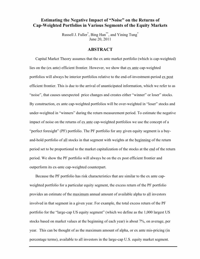
Estimating the Negative Impact of “Noise” on the Returns of

Cap-Weighted Portfolios in Various Segments of the Equity Markets

Russell J. Fuller*, Bing Han**, and Yining Tung* June 20, 2011

ABSTRACT

Capital Market Theory assumes that the ex ante market portfolio (which is cap-weighted)

lies on the (ex ante) efficient frontier. However, we show that ex ante cap-weighted

portfolios will always be interior portfolios relative to the end-of-investment-period ex post

efficient frontier. This is due to the arrival of unanticipated information, which we refer to as

“noise”, that causes unexpected price changes and creates either “winner” or loser” stocks.

By construction, ex ante cap-weighted portfolios will be over-weighted in “loser” stocks and

under-weighted in “winners” during the return measurement period. To estimate the negative

impact of noise on the returns of ex ante cap-weighted portfolios we use the concept of a

“perfect foresight” (PF) portfolio. The PF portfolio for any given equity segment is a buy-

and-hold portfolio of all stocks in that segment with weights at the beginning of the return

period set to be proportional to the market capitalization of the stocks at the end of the return

period. We show the PF portfolio will always be on the ex post efficient frontier and

outperform its ex-ante cap-weighted counterpart.

Because the PF portfolio has risk characteristics that are similar to the ex ante cap-

weighted portfolio for a particular equity segment, the excess return of the PF portfolio

provides an estimate of the maximum annual amount of available alpha to all investors

involved in that segment in a given year. For example, the total excess return of the PF

portfolio for the “large-cap US equity segment” (which we define as the 1,000 largest US

stocks based on market values at the beginning of each year) is about 7%, on average, per

year. This can be thought of as the maximum amount of alpha, or ex ante mis-pricing (in

percentage terms), available to all investors in the large-cap U.S. equity market segment.

Forthcoming, Journal of Investment Management

We thank the following who made many helpful comments on previous versions of this

paper: Shlomo Benartzi, David Jobson, Michael Klag, John Kling, Sylvia Kwan, Bill Sharpe,

Wei Su, Richard Thaler, Kent Womack, and two anonymous referees. All remaining errors and

omissions are ours.

______________________________________________________________________

*Fuller and *Tung are at Fuller & Thaler Asset Management, San Mateo, CA. **Han is at the University of Texas, Austin, TX.

1

Estimating the Negative Impact of “Noise” on the Returns of

Cap-Weighted Portfolios in Various Segments of the Equity Markets I. INTRODUCTION

Recently there have been several papers dealing with different concepts of market

efficiency.1 There is a long history in the financial economics literature, summarized by Fama

(1970, 1991), that dealt with what we will refer to as “fair-game” efficiency. Empirical tests of

“fair-game” efficiency essentially dealt with the question of whether active investment managers

“beat the market,” or more appropriately, “beat the appropriate benchmark” for the segment of

the equity (or bond) markets they are measured against. This paper deals with what we will call

“valuation” efficiency. That is, are current market prices set at t=0 such that the securities

actually provide the consensus expected return for the return measurement period, t=0 to t=1?

Does the consensus expected return for a security at t=0 equals the subsequent realized return

over the measurement period t=0 to t=1?

In financial theory the ex ante “market portfolio” is viewed as the portfolio that holds all

risky assets with portfolio weights based on the current market value of these assets, and it is

commonly assumed that the ex ante “market portfolio” lies on the ex ante efficient frontier.2 In

the practical world of equity investment management the concept of the ex ante “market

portfolio” is indirectly very important because most investment managers’ performance (ex post

returns) are measured relative to some index that typically is formed by using all (or most) of the

stocks in a particular segment of the equities market, and the initial weights of each stock in that

segment are typically based on each stocks’ relative market value at the beginning the

1 See Statman (2011) as one example.. 2 See Sharpe (1970) for a nice summary of the early literature on portfolio and capital market theory. See Markowitz (2005) for recent developments in this literature, and an argument that under more realistic assumptions, the market portfolio is not necessarily on the efficient frontier.

2

performance measurement period, t=0.3 (For example, two common proxies for the US large-cap

equity segment are the S&P 500 and the Russell 1000 index, and both indexes are, at any point in

time, ex ante cap-weighted indexes.)

We show that any ex ante, cap-weighted index for a particular equity segment will

always be an interior portfolio relative to the ex post measurement period efficient frontier for

that segment. The main reason for this is due to the arrival during the return measurement period

of new information that could not have been anticipated by the consensus of investors at the

beginning of the period. This new information can be “good,” for some companies, creating

“winner” stocks, for which the ex ante beginning of the period market-cap weighted segment

portfolio (or index) will be under-weighted, and vice versa for the arrival of unanticipated “bad”

news creating “loser” stocks. Simply put, ex ante cap-weighted segment portfolios will

inevitably be over-weighted in what turn out to be “loser” stocks and under-weighted in

“winners” during the ex post return measurement period.4 We will use the term “noise” to refer

to anything that causes unexpected changes in stock prices. For our purposes, it does not matter

whether these price changes are rational responses to genuine unanticipated information, or

irrational reactions to something else.5

This set-up allows us to ask, and provide a reasonable answer to the following question:

“How much is the ex ante cap-weighted segment portfolio an interior portfolio relative to the

segment’s ex post efficient frontier?” This is an important question for several reasons.

3 This is also generally true for investment managers in the bond markets and other segments of the capital markets that consist of tradable, risky assets. This paper focuses solely on various segmemts of the equity markets. These segments are relatively easy to identify and this helps avoid Roll's critique (1977) concerning the identification of the true market portfolio. 4 There is one unlikely exception to this result: If, over the return measurement period, all stocks in the segment generate exactly the return expected by the consensus of investors at t=0. Then there would be no “winners” or “loser” stocks, the segment would be perfectly valuation efficient, and the ex ante segment portfolio would plot on the ex post efficient frontier for the return measurement period. While this is conceptually possible, it strike us as extremely unlikely, and empirically this was not the case for any single year from 1951 – 2009 for the US Large-Cap Segment. (See Exhibit 1.) 5 Our usage of the term “noise” is very similar to Black’s (1986) use of the term “noise” in financial markets, as opposed to the irrational “noise” trader risk of De Long, Shleifer, Summers and Waldmann (1990).

3

• First, in the theory of finance, the concept of the ex ante market portfolio being the

tangency portfolio on the ex ante market efficient frontier which, when connected by

a straight line with the risk-free rate, creates the capital market line (CML), which is

an important concept for capital market theory.

• Second, to the extent the ex ante cap-weighted segment portfolio formed at t=0 is an

interior portfolio relative to the ex post efficient frontier at t=1, one has an estimate of

how “valuation” efficient that segment of the equity market was for the measurement

period in question. For example, if the market estimates for the values of each stock

were exactly correct at t=0 (this is the same as the estimates of the expected returns at

t=0 being exactly right for the return measurement period (t=0,1)), then the market for

that segment would be perfectly “valuation” efficient -- there will be no positive or

negative alpha stocks, and the ex ante segment portfolio at t=0 will be on the ex post

efficient frontier for the measurement period (t=0,1).

• Third, having a sensible estimate of how much the cap-weighted ex ante segment

portfolio is an interior portfolio relative to the ex post efficient frontier is important

for the actual practice of investment management because the ex ante segment

portfolio (usually some cap-weighted index such as the S&P 500) is frequently used

as a benchmark in selecting and evaluating active managers. If the ex ante segment

portfolio is only 1% below the subsequent ex post efficient frontier for the return

measurement period, it is unlikely that active managers in that segment and for that

time period will beat the segment benchmark, and it will be even more unlikely any

single manager will beat it by a large amount. On the other hand, if the ex ante

segment portfolio is 20% below its subsequent ex post efficient frontier, the

probability for a single manager significantly outperforming the benchmark is

considerably higher.

4

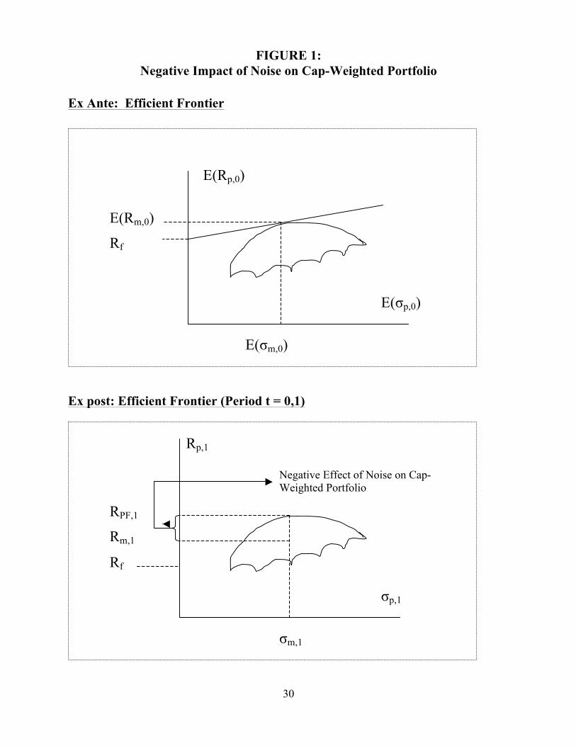
In Figure 1 below we use the notation E(Rm,0) to denote the expected return of the ex ante

cap-weighted market portfolio for segment S; Rm,1 to denote its realized return over the period

(t=0,1); and RPF,1 to denote the ex post return for the PF segment portfolio that has similar risk

characteristics as the Rm portfolio, but lies on the ex post efficient frontier – PF stands for

“perfect foresight,” a key concept we use to estimate how much the ex ante cap-weighted

portfolio is an interior portfolio relative to the ex post segment efficient frontier. Figure 1

illustrates that although the ex ante segment portfolio is on the ex ante efficient frontier at t=0, it

will be below the ex post efficient frontier for period (t=0,1).

{Place Figure 1 approximately here}

II. A SIMPLE METHOD FOR ESTIMATING THE NEGATIVE EFFECT OF “NOISE” ON CAP-WEIGHTED PORTFOLIO RETURNS

Our simple method to estimate an upper bound for the negative impact of noise on the ex

post return, and therefore the valuation efficiency of an ex ante cap-weighted market/segment

portfolio, depends upon two critical assumptions:

• Most important is the concept of perfect foresight (PF).6 Given that the PF

portfolio knows the end-of-period weights, it also must know the precise return

for the period of all stocks in the segment. Thus it should be clear that the

difference in returns between a PF segment portfolio and the ex ante cap-weighted

portfolio (at t=0) is an upper bound for the total excess return potentially available

to active managers in a particular equity segment.

• Second, by concentrating on specific segments of the equity markets, we avoid

the problem of defining the market portfolio. For example, arbitrarily defining the

6 Our definition of “perfect foresight” is similar in spirit, but different empirically from Shiller (1979, 1981), LeRoy and LaCivita [1981] and Arnott, et.al. [2009].

5

1,000 largest US stocks based on market values at the beginning of each year as

the “large-cap US equity segment,” our estimate of the total negative effect of

cap-weighting on the ex ante large-cap US segment portfolio per year is

approximately 7% of the total beginning of the year market-values of these

stocks.

The following summarizes the notation we use:

• MPS,0 = the ex ante portfolio that holds all stocks in segment S with initial

weights proportional to the market values of all stocks in S at the beginning of the

period.

• R(MPS,1) = the realized, ex post return on portfolio MPS,0 over the period (t=0,1).

• PFPS,0 = a portfolio that holds all stocks in segment S with initial weights

proportional to the market values of the stocks in S at the end of the period

because it has perfect foresight. (PF is obviously an artificial construct because

no one can have perfect foresight.)

• R(PFPS,1) = the realized, ex post, return on PFPS,0 over the period t=(0,1).

Both MPS,0 and PFPS,0 are buy-and hold portfolios over the period t=0 to 1. Leverage and

short selling are not allowed in MPS,0 and PFPS,0, although these assumptions are not technically

necessary to obtain our segment-level results, which are what we report. Any individual investor

in segment S can earn practically any return, depending upon how many stocks they hold long

and short, how much leverage is involved and how skilled (or lucky) they are. But, as a group, all

investors involved in segment S must hold all stocks in proportion to their market values at any

point in time, except for the PF investor, who we implicitly assume has no impact on prices.

In the Appendix A we show analytically that the ex-ante market portfolio always lies

below the ex-post efficient frontier and the perfect foresight portfolio always outperforms the ex-

ante segment portfolio. Active fund managers with relevant information about future stock

returns that is not reflected in the current stock prices would tilt their portfolios towards our

6

perfect foresight portfolio, but in aggregate they could never attain the excess return of the PF

portfolio.

In the Exhibits at the end of the paper we show empirically that for the US Large-Cap

Equity Segment the annualized total volatility for MPS,0 and PFPS,0 are nearly identical and that

the betas and correlations between the two portfolios are very close to 1.0. Thus, we estimate the

negative effect of “noise” on the ex ante cap-weighted portfolio’s ex post return (expressed as a

percentage of beginning total market values) in segment S during the return measurement period

as the difference between the returns of the PF portfolio and the ex ante cap-weighted portfolio.

We refer to this difference as simply the “excess return” of the PF portfolio for segment S.

(1) Excess return = R(PFPS,1) - R(MPS,1).

Conceptually, the difference between the realized return of the ex ante cap-weighted

segment portfolio for a particular segment and that of a portfolio on the ex post efficient frontier

for that segment and that has similar risk characteristics, provides an estimate of the total amount

of excess return available to all investors in segment S, expressed as a percentage of the

beginning of the period market value of the segment. Because the risk-characteristics of the ex

ante segment portfolio (MPS,0) for any segment S, and the PFPS,0 are so similar, our estimate of

the total amount of “excess return” can also be thought of as an estimate of the maximum annual

amount of alpha in Segment S, available to all investors involved in segment S in a given year.

For example, if the excess return difference is 7% and the market value of the segment at t=0 is

$1billion, then the maximum amount of “excess return,” or alpha, in dollars that is available to

all participants is approximately $70 million during the measurement period, which we define

arbitrarily as calendar years.

We have focused on price changes occurring during the period t=(0,1) due to the arrival

of information that is important for pricing, but could not have been anticipated by the consensus

7

of investors in segment S at t=0. We recognize that there could be other factors affecting

realized stock returns. For example, some stocks may not be ex ante “valuation efficient.”

Suppose there is mispricing at the beginning of the period that non-PF investors could identify ex

ante. An example might be the so-called value premium. To the extent one believes there is a

“true” value premium of, say, an average of 2% per year, then one would want to subtract 2%

from our estimate of the maximum negative effect of “noise” on cap-weighted portfolios.

Obviously the “value” premium is based on knowing the ratio of book value to price at t=0, two

data items available to any interested investor. If enough investors believe in the value premium,

it should be correctly imbedded in prices at t=0, i.e., arbitraged away, unless it is “risk”.

While our estimates of the negative impact of noise on cap-weighted portfolios represent

a maximum and therefore are overstated, we believe any “true” empirical anomalies and

possibly truly superior forecasting ability by a few investors relative to the entire set of investors

in segment S are small enough to be ignored for the purpose of this paper.

III. EMPIRICALLY ESTIMATING THE AMOUNT OF “EXCESS RETURNS” IN

VARIOUS SEGMENTS OF THE EQUITY MARKETS

To estimate the amount of excess returns as a percentage of various segments of the

equity markets, we used the following procedures and assumptions:

1. We constructed our own paper-indexes that are representative of various segments

of U.S. stocks, as well as large-cap EAFE stocks. In general terms, we followed

the methodology used in constructing the CRSP indices.7

2. The US data was taken from the CRSP data sets. For non-US stocks, the data was

taken from MSCI EAFE Index data sets.

3. The return measurement periods were set as annual calendar years for t=0 to 1.

7 The specific methodology for this procedure is described in detail in Fuller, Han and Tung (2010).

8

4. As of December 31 of each calendar year stocks in the data sets were ranked from

1 to N (where N is the total number of stocks in the data sets as of December 31

of each calendar year), based on each stock’s market value.

5. The segment denoted “large-cap US stocks” consisted of stocks ranked 1 to

1,000; the stocks denoted “mid-cap US stocks" consisted of stocks ranked 1,001

to 2,000; the stocks denoted “small-cap US stocks” consisted of stocks ranked

2,001 to 3,000. (For completeness, we also defined a US small-cap segment as

stocks ranked 1,001 to 3,000 which roughly match the Russell 2000 index.)

6. For non-US stocks, we simply used all the stocks in the MSCI EAFE Index data

set that are designated as “large-cap.” Thus, the number of stocks in this segment

varied for any single year as the MSCI EAFE Index data set expanded over time.

7. Paper-indexes obviously do not include transaction costs. However, real

portfolios that are indexed to paper-indexes do have transaction costs, even

though they are buy-and-hold portfolios for the time periods (calendar years in

this study) because of intermittent cash flows from cash dividends and certain

corporate transactions including stock splits, repurchases, mergers and

acquisitions. For the US large-cap segments we used 40bps for one-way total

transaction costs (commissions, market impact, etc.); for the US mid-cap segment

we used 80bps for one-way transaction costs, as well as for stocks 1,001 to 3,000

(essentially equivalent to the R2000 index); for the US small-cap segment (stocks

2,001 to 3,000) and for EAFE we used one-way 85bps transaction costs. Thus

Exhibit 1 and most of the other Exhibits report returns both before and after

transaction costs (TC) for both the segment benchmark (MPS,,t) and the segment

PF portfolio (PFPS,,t).

9

In Exhibit 1 the time period for large-cap US stocks includes the calendar years 1951

through 2009, 59 years inclusive. The choice of 1951 as the starting year is because December

31, 1950 was the first year-end for which CRSP has at least 1,000 stocks. 1973 was chosen as the

starting year for the other US stock segments because this was the first year CRSP lists 3,000 or

more stocks. Beginning with Exhibit 6 we use 1973 as the starting year for all US segments and

EAFE large-cap stocks to be consistent so that all segments have the same start date.

IV. EMPIRICAL RESULTS FOR THE US LARGE-CAP SEGMENT, 1951 – 2009

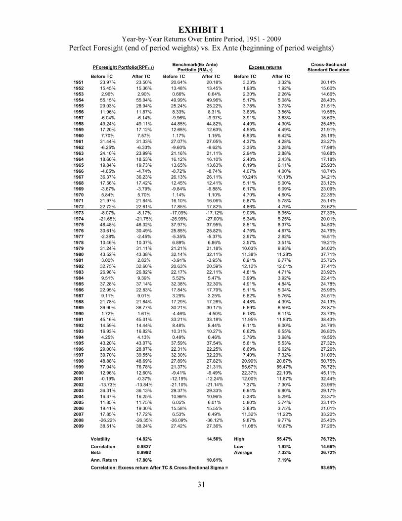
Exhibit 1 (and Exhibits 2, 3, 4, and 5) are based on the full 59 year period, 1951 -2009

inclusive, for the equity segment we designate as US Large-Cap. Note in Exhibit 1 that we have

drawn a line after 1972, as we only present results for the four other equity market segments we

examined from 1973 onward – in general, returns in the years 1951 – 1972 are less volatile than

in the subsequent time period, 1973 – 2009.

{Place Exhibit 1 Here}

In Exhibit 1, the column of most interest is the Excess return (After TC), which is our

estimate of the ex post “excess return”, R(PFPS,1) - R(MPS,1) for the US Large-Cap segment.

First, note that each year the excess return is positive, as “perfect foresight” should always be

valuable and has to be, by construction, using our methodology.

Note also the summary statistics at the bottom of the column: the high is a rather stunning

55.47% (1999), the low is 1.92% (1952) and the annualized excess return over the 59 years is

7.19%.8 Also note that the volatility (standard deviation of annual returns, bottom of column 2)

for the large-cap US “perfect foresight” portfolio, σ(RPFPS,1), is 14.82% compared to the

volatility for the benchmark (ex ante Segment Portfolio) of 14.56% (bottom of column 4), and

8 Compound annualized returns (geometric mean returns) will always be lower than the simple average of returns (7.32%) if there is any variance in the return time series.

10

the correlation between the two return series is 0.9827 (bottom of column 2), which results in a

beta of 0.9992 for R(PFPS,1) relative to R(MPS,1), after transaction costs. The similar risk

characteristics should not be surprising because the two portfolios hold the same 1,000 stocks at

the beginning of each year, with the difference being the ex ante market portfolio holds these

stocks based on the their beginning of the year market values and the PF portfolio holds these

stocks at the beginning of the year based on their end of the year market values. Particularly for

large-cap stocks, it seems reasonable that weights based on beginning and end of the year market

values should be highly correlated, and they are. In this case, the correlation coefficient (not

reported in Exhibit 1) is 0.978.

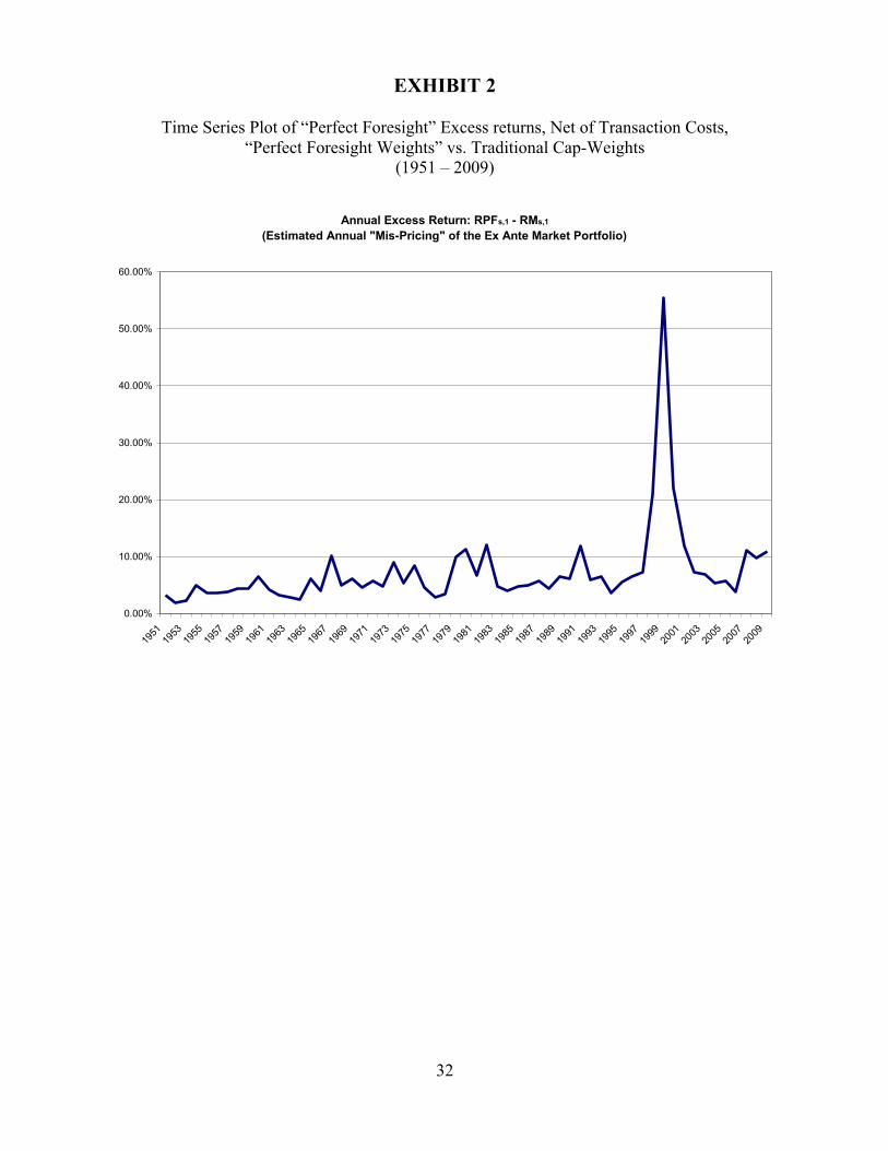
Exhibit 2 plots the time series of the PF portfolio’s yearly excess return after transaction

costs (column 6 in Exhibit 1) simply to illustrate the volatility of the year-by-year excess

returns, or what we refer to as the estimated annual ex post “excess return” for the PF portfolio

versus the ex ante US large-cap equity segment due to “noise” or simply price changes.

{Place Exhibit 2 Here}

An interesting question is: “What causes the year-by-year ex post “excess return” to be so

volatile?” The last column of Exhibit 1 lists the year-by-year cross-sectional standard deviation

of the 1,000 largest market value US stocks returns by year. Just by looking at the last two

columns in Exhibit 1, it is easy to see they are highly correlated time series.

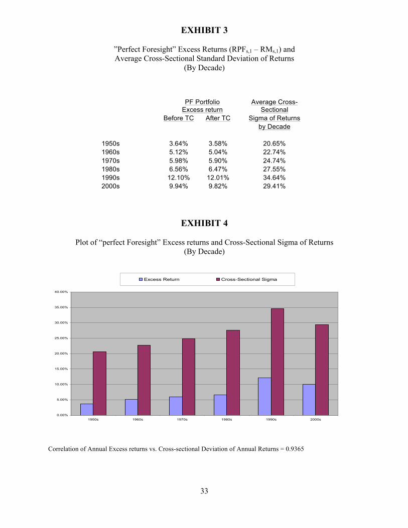
Exhibit 3 makes this clearer by presenting averages by decades of the “perfect foresight”

portfolio’s estimated excess returns of the PF portfolio for the US large-cap Equity segment and

the cross-sectional standard deviation of returns for the top 1,000 US stocks. It is easy to see

from Exhibit 3 that the higher the average cross-sectional dispersion of returns for the top 1,000

US stocks, the greater the PF portfolio’s estimated excess return in this segment of the equity

markets.

{Place Exhibits 3 & 4 Here}

11

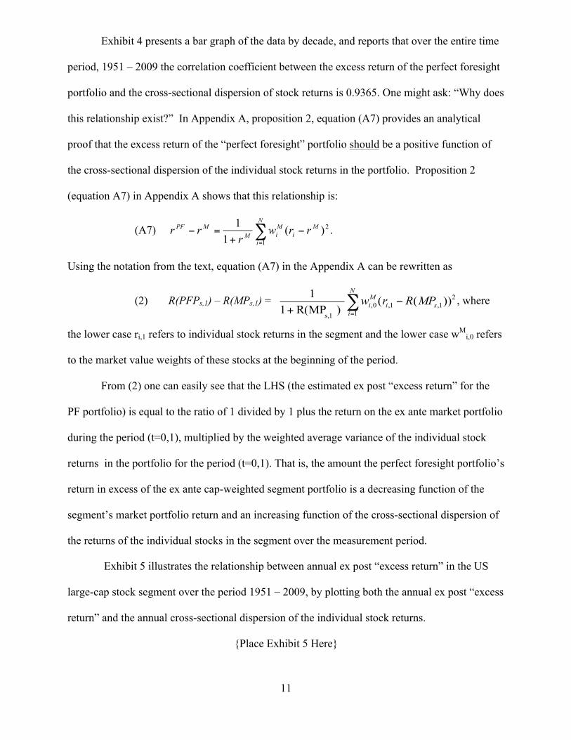
Exhibit 4 presents a bar graph of the data by decade, and reports that over the entire time

period, 1951 – 2009 the correlation coefficient between the excess return of the perfect foresight

portfolio and the cross-sectional dispersion of stock returns is 0.9365. One might ask: “Why does

this relationship exist?” In Appendix A, proposition 2, equation (A7) provides an analytical

proof that the excess return of the “perfect foresight” portfolio should be a positive function of

the cross-sectional dispersion of the individual stock returns in the portfolio. Proposition 2

(equation A7) in Appendix A shows that this relationship is:

(A7) 2

1

)(11 M

i

N

i

MiM

MPF rrwr

rr −+

=− ∑=

.

Using the notation from the text, equation (A7) in the Appendix A can be rewritten as

(2) R(PFPs,1) – R(MPs,1) = 21,1,

10,

s,1

))(( )R(MP1

1si

N

i

Mi MPRrw −

+ ∑=

, where

the lower case ri,1 refers to individual stock returns in the segment and the lower case wMi,0 refers

to the market value weights of these stocks at the beginning of the period.

From (2) one can easily see that the LHS (the estimated ex post “excess return” for the

PF portfolio) is equal to the ratio of 1 divided by 1 plus the return on the ex ante market portfolio

during the period (t=0,1), multiplied by the weighted average variance of the individual stock

returns in the portfolio for the period (t=0,1). That is, the amount the perfect foresight portfolio’s

return in excess of the ex ante cap-weighted segment portfolio is a decreasing function of the

segment’s market portfolio return and an increasing function of the cross-sectional dispersion of

the returns of the individual stocks in the segment over the measurement period.

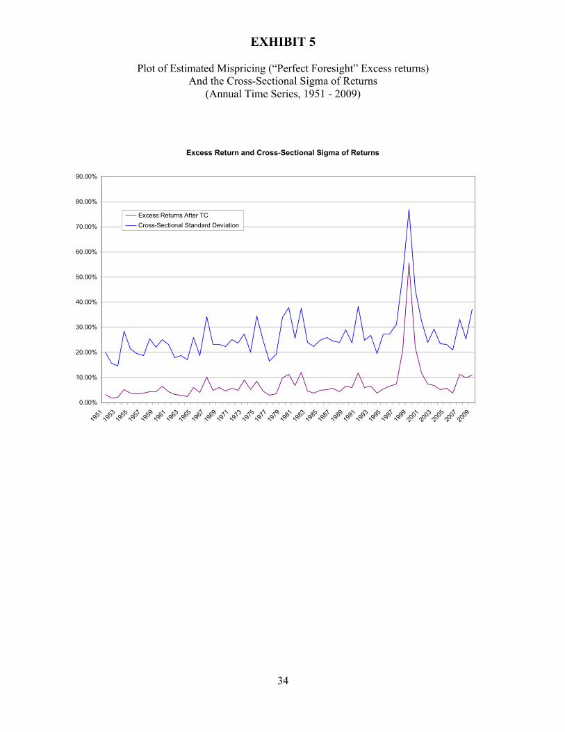
Exhibit 5 illustrates the relationship between annual ex post “excess return” in the US

large-cap stock segment over the period 1951 – 2009, by plotting both the annual ex post “excess

return” and the annual cross-sectional dispersion of the individual stock returns.

{Place Exhibit 5 Here}

12

Intuitively, this general relationship should be obvious. For example, imagine a year

when every stock has the same return, say, 6%. In that year, every portfolio will also have the

same return (even a single stock portfolio), including the ex ante segment portfolio. And, the

cross-sectional standard deviation of individual stock returns in the segment will, obviously, be

zero. One can easily see from equation (2) that, holding the segment return constant, the larger

the variance of the cross-sectional of individual stock returns in the segment, the larger will be

the value of perfect foresight and the amount of estimated ex post excess return of the PF

portfolio relative to the ex ante market portfolio for the segment.

Another interesting feature about our estimate of the amount of excess return in the large-

cap US segment is that it can easily be converted into an estimate of the potential maximum total

dollars of alpha (positive and negative) available to all investors in the large-cap U.S. equity

space.9 For example, if the market-value of the top 1,000 U.S. stocks at the beginning of a year is

$1 trillion, then assuming our estimate of the maximum possible alpha of 7.19% is reasonable,

simply multiply $1 trillion by 7.19% and the estimate of the potential maximum total dollars of

alpha in this segment available to all investors is $72 billion. Thus, the “holy grail” of investing

(being able to approach perfect foresight) is certainly worth pursuing, but at the same time, one

wants to treat such a number (for example, the $72 billion of potential total alpha noted above)

with a great deal of caution for several reasons:

• First, it represents a maximum across all investors in the segment – surely no

single investor, or group of investors, will ever have perfect foresight, as we

defined this concept.

9 Generally speaking, the sum of the alphas in a sector should equal zero, as one investor’s abnormal gain should be other investors’ abnormal loss. However, the sum of the absolute value of the alphas will always be a positive number. Since the PF portfolio is over-weighted in the winners and under-weighted in the losers, it’s positive excess return, in dollars, is equivalent to the sum of the absolute values of the alphas in its particular equity segment.

13

• Second, for an investor to achieve higher abnormal returns, that investor will

probably have to incur higher turnover and transaction costs. Also, for an investor

to achieve higher abnormal returns, that investor will probably have to own a

more concentrated portfolio, thus assuming more risk.

• Third, and most important, one must bear in mind that surely a significant amount

of our estimates of ex post excess return in various equity market segments is due

to the arrival of information that simply cannot be anticipated, and therefore is not

exploitable by active management strategies. It is an interesting question as to

how much of the PF portfolio’s excess return is truly not anticipatable, which we

leave for future research.

In the ongoing debate over the value of active management, the “answer” probably lies in

one’s belief structure. Those who believe markets are (or are nearly) perfectly efficient will

believe the answer is zero, or close to zero, and they should probably index their portfolios to

benchmarks for various market segments.

Those who believe in active management should still use realistic expectations of what is

achievable. For example, if our estimate of the amount of ex post excess return for the large-cap

US equity segment of 7% is reasonably close to the correct number, then it seems to us that one

should expect superior active managers in this segment to earn on average less than, say, half of

this amount, (2-3% per year). In other words, one should be realistic about what active

management can achieve in the large-cap US equity segment.

It is also the case that empirically, most studies have found active managers to

underperform their benchmarks.10 Almost all benchmarks that are used to evaluate equity

10 There is a large empirical literature that generally finds zero to negative alpha associated with most active management strategies – most of these studies have concentrated on mutual funds because of data availability. See Barras, Scaillet and Wermers [2010] for a recent study that summarizes much of the previous literature and presents a new empirical technique for conducting tests for alpha and finds resultants similar to the many previous papers. For example, according to the research firm Morningstar, only 32 percent of actively managed funds specializing in American stocks beat the return of the Standard & Poor's 500-stock index in 2006. The Wall Street Journal (April

14

managers are cap-weighted and cap-weighted benchmark returns suffer what seems to us to be a

quite large negative effect due to “noise”, or even more simply, to price changes. At first glance

this struck us as puzzling because active managers do not outperform, on average, their

benchmarks, despite the large negative effect of noise on cap-weighted benchmarks. However, it

seems plausible that many actively managed portfolios are weighted in a manner that is close to

cap-weighting.11 If this is so, then their portfolio returns would, on average, suffer roughly the

same negative return effect caused by “noise”.

Consequently, it is easy to make a strong case for traditional, cap-weighted indexing as a

sensible investment strategy, despite the fact that the paper index used as a benchmark is

constructed based on a number of arbitrary, active decisions12. It will be a low-cost form of

investing and it will provide a well diversified portfolio that also has relatively low-risk relative

to the benchmark that is chosen to be representative of the segment of the equity markets the

investor wants exposure to.

V. ESTIMATES OF THE AMOUNT OF EX POST EXCESS RETURN IN

VARIOUS EQUITY MARKETS SEGMENTS, 1971 - 2009

Appendix B and its corresponding exhibits (Exhibits7 –11) report results for estimating

the amount of ex post “excess return” for ex ante segment portfolios in five different segments of

the equities markets – large-cap US stocks, large-cap EAFE stocks, mid-cap US stocks, and

small-cap US stocks. For ease of comparison, all of the results for these exhibits are reported in a

22, 2009) reported a new study from Standard & Poor's that finds 70% of large-cap fund managers who use the S&P 500 as a benchmark for comparison have failed to match the performance of the index over the past five years. Sharpe [1991] argues that active managers trade among themselves but collectively they must resemble an index fund. Hence, after subtracting transaction costs, the average actively managed portfolio must under-perform the average indexed portfolio. 11 Recent studies document that actively managed funds are reluctant to deviate from the market portfolio, or the benchmark they are expected to beat. See Lakonishok, Shliefer and Vishny (1997), Chan, Chen and Lakonishok (2002), and Cohen, Gompers and Voluteenaho (2003). 12 See Fuller, Han and Tung (2010) for a discussion of how many active decisions are involved in constructing indexes, such as the S&P 500 or the Russell indexes, which are commonly used as benchmarks in the investment strategy known as “indexing.”

15

similar format and for the same time period, the 27 calendar years 1973 – 2009 inclusive -- the

time period for which sufficient data is available for each segment.

For the US stocks, our definition of large-cap remains the same, the top 1,000 stocks –

that is, stocks ranked from 1 to 1,000 based on beginning of the year market values; mid-cap

stocks are defined as stocks ranked from 1,001 to 2,000 and small-cap stocks are defined as

stocks 2,001 to 3,000, again based on beginning the year market values. (Simply for the purpose

of completeness Exhibit10 reports results for stocks 1,001 to 3,000 which are nearly identical to

the popular “Russell 2000” small-cap index.) For the large-cap EAFE stocks (Exhibit 8) we use

all stocks that are in the MSCI EAFE large-cap index at the beginning of each year13.

Because the results are similar to those in Exhibit 1, we place Exhibits 7-11 in Appendix

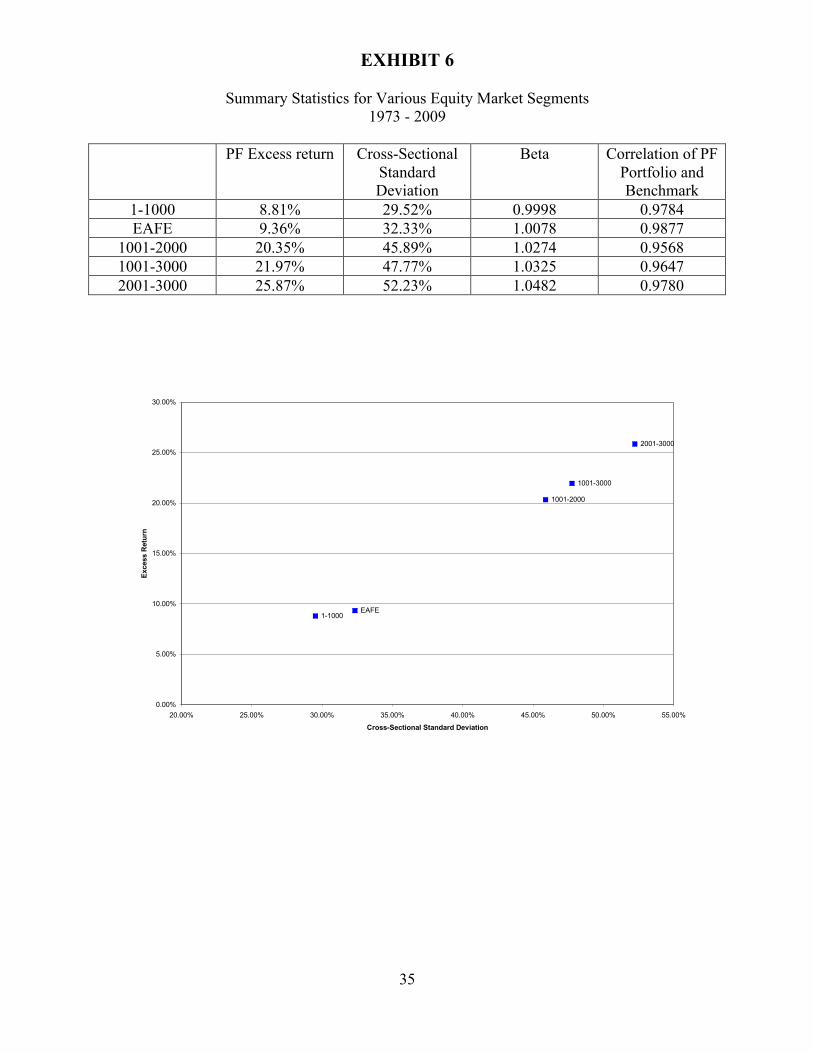
B, with additional comments on their results. Exhibit 6 below summarizes the results in Exhibits

7 -11in Appendix B.

{Place Exhibit 6 here}

Note in Exhibit 6 that as one moves down in market-cap size from the large-cap US

segment (the top 1,000 stocks) to the smallest (stocks 2,001 to 3,000), the average estimated ex

post excess returns of the PF segment portfolios for each of the segments increases

monotonically, from 8.81% to 25.87% (column 2). The average cross-sectional dispersion

(standard deviation) of the individual stock returns in these segments also increases

monotonically from 29.52% to 52.23% (column 3). This relationship is graphed at the bottom of

Exhibit 6.

In general we find that the smaller the average capitalization size in a segment of the

equity market, the greater the cross-sectional standard deviation of returns for stocks in that

13 The MSCI EAFE Index file actually has complete data starting at the end of 1969 – thus, we excluded 3 years of return data for EAFE in order to have a consistent starting date for the data in Exhibits76 – 11. Including the extra 3 years (1970 – 72 inclusive) does not change the EAFE results reported in Exhibits 7 and 11 materially. For the years 1973 – 2009 the number of stocks in the EAFE large-cap index ranged from 762 to 1,211, and generally (but not always) increased over time as new stocks were added to the index and occasionally stocks were deleted due to takeovers, bankruptcies and other corporate actions.

16

segment, and the greater the negative impact of price changes on the cap-weighted portfolios.

Also, we note that the EAFE large-cap segment has, on average, a smaller capitalization over the

period 1973-2009 than the US large-cap segment, a higher cross-sectional dispersion of returns

and a correspondingly greater negative impact on cap-weighted large-cap EAFE portfolios than

the large-cap US segment.

Finally, note that although the beta for each PF portfolio, relative to its segment of the

equity market, increases as the cap-size decreases, the betas are all still relatively close to 1.0,

and the correlations between the PF portfolios and their ex ante segment portfolios are all above

0.95. Thus, the PF portfolios, as constructed, have risk characteristics that are close to the

appropriate ex ante cap-weighted segment index or portfolio. (See Appendix B for additional

comments on these segments of the equity market.)

VI. SUMMARY AND THE CHALLENGE

In this paper we have proposed a simple method of estimating the negative effect of noise

on cap-weighted portfolios in various segments of the equity markets. Our methodology is based

on the concept of a perfect foresight (PF) portfolio, which is a portfolio holding long positions in

all stocks in the given equity segment with beginning weights proportional to the market

capitalization of the companies in the segment at the end of the investment period. (Obviously no

one knows precisely the future market value of each stock in the segment, so our estimates

should be considered the maximum that can be expected for the ex post excess return associated

with perfect foresight in each of the respective equity segments.) Our estimate of the average ex

post excess return for the PF portfolio in the U.S. large-cap segment of the capital markets,

defined as the largest 1,000 stocks based on their market values at the beginning of each year,

falls in the 7-9% range, depending upon the time period. The large-cap EAFE stocks are similar

to the large-cap US stocks, with the average ex post excess return being slightly larger. Our

17

estimate for the average amount of ex post excess return for the PF portfolios in the U.S. mid-cap

segment (defined as stocks 1,001 to 2,000) and the small-cap segment (stocks 2,001 – 3,000)

increases monotonically as one moves down the market-cap range.

In Appendix A we show analytically that our definition of the negative effect of noise on

cap-weighted portfolio returns in each particular segment is a positive function of the cross-

sectional dispersion of individual stock returns in the equity segment of interest in any particular

year. Our empirical results strongly confirm this relationship. However, caution is in order: We

use the term estimated ex post excess return because the risk characteristics for the perfect

foresight portfolios in the various segments, while close to the risk-characteristics for the ex ante

market portfolio for the same segment, they are not identical. Nevertheless, our estimates of the

amount of ex post excess return in various capital market segments provide a reasonable answer

to the old question in Capital Market/Asset Pricing theories of how much the ex ante market

portfolio will be an interior portfolio relative to the ex post efficient frontier, at least with respect

to various equity segments.

However, the CHALLENGE to active managers is not to show that the ex ante cap-

weighted segment portfolio will be an interior portfolio relative to the ex post segment efficient

frontier. The challenge is to show that they can consistently beat the ex ante cap-weighted

portfolio or index – what we refer to as “fair game” efficiency (can you beat the market?), as

opposed to the concept of “valuation efficiency” that is related the amount of ex post excess

return that is the result of ex ante mispricing due to noise. While we have shown that there is a

significant negative impact created by noise on the returns of ex ante cap-weighted portfolios,

this does not mean any particular active manager can beat their particular segment of the equity

markets.15 While there may be significant “valuation” inefficiency in various segments of the

equity markets, most of the commonly available data does not support the notion that the average

15 We do show in Fuller, Han and Tung (2010) that using only known market values (ex ante) of large-cap US stocks, one can beat the market-cap weighted large-cap index by 15-20 basis points per year after transaction costs.

18

active manager does “beat the market,” as suggested by many mutual fund studies and the data in

consultants’ databases of manager relative performance. Thus, while our evidence shows the

equity markets are not “valuation” efficient relative to having perfect foresight, our evidence

also does not suggest, (one way or the other) whether the equity markets are “fair game” efficient

– i.e., can you beat the market. The challenge to active managers is to prove they can.

Unfortunately, perfect foresight, like the fountain of youth, is probably something that

cannot be achieved or found. Thus, we believe one should not expect the average active manager

to achieve excess returns remotely close to our estimates of the amount ex post excess return in

various segments of the equity markets. However, by having these estimates, consultants, plan

sponsors and individual investors can form more reasonable estimates of what might be

achievable by active management.

19

APPENDIX A

Proposition 1: Proof that the Perfect Foresight Portfolio Lies on the Ex Post Efficient Frontier

In this Appendix A we use notation that is, in some cases, different from that used in the

text, in order to make the proofs more succinct.

There are N stocks Ni ,,2,1 = . For simplicity, assume their payoffs are uncorrelated

(we are not concerned with diversifications among stocks). Suppose uninformed investors

believe all stocks have the same expected return µ and standard deviationσ . Then the equal

weighted market portfolio is optimal from the perspective of the uninformed investors. Suppose

there is a set of informed investors (active-fund managers) who have access to private signals on

future stock returns. The active fund managers’ expected stock returns differ from those of

uninformed investors. Denote the expected return on stock i by [ ]iA rΕ .

Below we examine the optimal portfolio of active fund managers. Intuitively, their

portfolio would deviate from the market portfolio or the portfolio of uninformed investors, titling

towards stocks for which they expect higher returns (e.g., they have positive private signals).

However, in reality, active fund managers are constrained in their ability to transfer their

information into portfolio positions. In particular, they are often subject to both explicit and

implicit tracking-error constraints in their investment decisions. The explicit tracking-error

constraint as specified in investment contracts restricts the maximal possible deviation of a

money manager's portfolio from a given benchmark. Violation of such constraint can result in

termination of contract and lawsuits. The implicit tracking-error constraint arises from the

relative performance compensation, or the risk of being wrong and alone, popularly recognized

as the “maverick risk”.

20

Therefore, we study how an active fund manager chooses an all-stock portfolio by

maximizing expected return subject to a tracking-error constraint.16 This constraint requires that

the standard deviation of the manager’s return relative to the market portfolio does not exceed a

bound η . Specifically, the manager chooses portfolio weights Niwi ,,1, = to maximize the

expected return

⎥⎦

⎤⎢⎣

⎡Ε ∑

=

N

iii

A rw1

subject to ∑ ==

N

i iw1 1 and 21

))((Var η≤−∑ =

N

i iii rew , where ie is the weight of stock i in the

market portfolio M. The active manager's optimal portfolio choice and expected outperformance

of his optimal portfolio over the market portfolio are given below.

An active manager's optimal portfolio weight in stock i is

[ ]σ

η ][rbarrS

ew iA

ii−Ε

⎟⎠

⎞⎜⎝

⎛+= , (A1)

Where rbar is the cross-sectional mean of the expected stock returns, and S is a constant

describing the cross-sectional dispersion in the expected stock returns:

[ ] [ ]( )∑=

−Ε=N

ii

A rbarrS1

2 . (A2)

The excess expected return of his portfolio over the market portfolio is proportional to the cross-

sectional dispersion in the expected stock returns

SrrwN

iMii

A

ση

=⎥⎦

⎤⎢⎣

⎡−Ε ∑

=1

. (A3)

Proof: The Lagrangian of the constrained optimization is

⎥⎦

⎤⎢⎣

⎡−+⎥

⎦

⎤⎢⎣

⎡−−+⎥

⎦

⎤⎢⎣

⎡Ε= ∑∑∑

===

N

ii

N

iiii

N

iii

A wrewrwL1

21

21

11))((Var ληλ .

16 In the empirical part of this paper, we also consider other constraints faced by the managers. For example, they need to hold all stocks in equity segment portfolio and cannot short stocks.

21

The first order condition with respect to iw is

[ ] 0)(2 22

1 =−−−Ε λσλ iiiA ewr . (A4)

Summing (A4) over Ni ,,1 …= and using the fact that∑ ==

N

i iw1 1, we find that the Lagrangian,

multiplier, λ 2, is equal to the cross-sectional mean of the expected stock returns:

[ ] rbarNriAN

i=Ε=∑ =

/12λ .

Substituting this equation into (A4), we get

[ ]( )][21

21

rbarrew iA

ii −Ε+=σλ

. (A5)

We can solve for 1λ using (A4) and the tracking error constraint:

ησ

λ21S

= ,

where

[ ]( )∑=

−Ε=N

ii

A rbarrS1

2][

The optimal weight iw given in the Proposition 1 is obtained by substituting the expression for

1λ back into (5). The expression for the excess expected return ⎥⎦

⎤⎢⎣

⎡−Ε ∑

=

N

iMi

A rw1

follows

straightforwardly from (A1).

Two observations are noteworthy from Proposition 1. First, informed investors would

deviate from the market portfolio by overweighting (underweighting) stocks they have positive

private (negative) information about, or stocks they view as undervalued (overvalued) with

respect to their information set. Second, their expected outperformance over and above the

market portfolio is proportional to the cross-sectional dispersion in the expected stock returns.

Intuitively, when the cross-sectional dispersion in the expected stock returns is high, private

22

information is more valuable, and the informed investors have more opportunities to profit from

their information advantage.

Comments:

So what is the maximum expected out-performance by the active fund managers in

aggregate?17 This is an important question to both academic researchers and practitioners, but it

is difficult to answer. The problem is that empirically, active managers’ private information is

unobservable to researchers. Thus, it is impossible to exactly quantify the expected gain from

their information advantage.

We attempt to address estimate the maximum “alpha” available to the active fund

managers in the aggregate by constructing a proxy of the aggregate informed investors’ portfolio.

Our proxy is motivated by the following observation. If an active manager has an informational

advantage, stocks that these active fund managers are more bullish about (i.e., [ ] µ>Ε iA r ) on

average tend to have higher ex-post realized returns. On the other hand, stocks that active fund

managers are more bearish about (i.e., [ ] µ<Ε iA r ) tend to have on average lower ex-post realized

returns.

Proposition 2: The Excess Return for the Perfect Foresight Portfolio is a Positive Function of the Cross-Sectional Variance of the Individual Stock Returns in the Segment

Thus, we use the ex-post realized stock returns to proxy for private information that

active fund managers possess. Of course, the ex-post realized stock returns over a period are

foresight from an ex-ante perspective (at the beginning of the period). To measure the maximum

“dollar amount of alpha” defined as the average ex post “excess return” of the ex ante market

portfolio multiplied by the beginning of the period market value of the equity segment of

interest, we assume “perfect foresight” in the sense the market capitalization of each stock at the

17 We are only interested in the aggregate dollar amount of alpha, or the average excess return, that is available to active fund managers. Obviously, active fund managers are heterogeneous as they have access to different signals, and use different investment techniques, or follow different sets of stocks. Some of them would have higher alpha (excess return) while others have lower alpha than the average excess return we try to estimate.

23

end of the period is assumed to be known to someone at the beginning of the period. We define

the Perfect Foresight portfolio to be a value-weighted portfolio of all stocks in our universe with

initial weights proportional to the market capitalization of the stocks at the end of the period.

To fix notations so that they are more succinct, denote the market capitalization of stock

i at the beginning of the year by 0iM and stock return over the year by ),,1(, Niri = . By

definition, its market capitalization 1iM at the end of year is 01 )1( iii MrM += . Consider two

portfolios. The first portfolio (M ) is a value-weighted index of the N stocks with weights

proportional to each stock’s market capitalization at the beginning of the year. Its return over the

year is

∑=

=N

ii

Mi

M rr1

ω , where ∑=

=N

jji

Mi MM

100 /ω .

The second portfolio, the perfect foresight portfolio ( PF ) consists of the same N stocks, except

the weights are proportional to stock's market capitalization at the end of the year. Its return over

the year is

∑=

=N

ii

PFi

PF rr1

ω , where ∑=

=N

jji

PFi MM

111 /ω

By definition,

MiM

iN

j j

N

j j

N

j j

i

i

iPFi r

rM

M

MM

MM

ωω+

+==

∑∑

∑ =

=

=1

)1(

1 1

1 0

1 0

0

0

1 .

Thus, the difference in the portfolio weights between the perfect foresight portfolio and the

market portfolio is

)(1

MiM

MiM

iPFi rr

r−

+=−

ωωω (A6)

The difference between the realized returns of the two portfolios is

24

∑=

−=−N

ii

Mi

PFi

MPF rrr1

)( ωω

Plugging (A6) into MPF rr − , we have

MPF rr − ∑=

⎟⎠

⎞⎜⎝

⎛−

+

+=

N

iiM

iMi r

rr

1

11

)1(ω

∑=

−+

=N

ii

Mi

MiM rrr

r 1

)(11

ω

∑∑==

−+

+−+

=N

i

Mi

MiM

MN

i

Mi

MiM rr

rrrr

r 11

2 )(1

)(11

ωω

∑=

−+

=N

i

Mi

MiM rr

r 1

2)(11

ω . (A7)

which is the same as the simplified equation (2) in the text. Thus, regardless of what the realized

stock returns ir are, the portfolio PF always has higher return than the portfolio M . Equation

(A7) also shows that the return difference of these two portfolios is proportional to the weighted

cross-sectional dispersion of stock returns (i.e., standard deviation of { } Niir ,,1=, giving M

iω

weight to the observation ir ).

The following summarizes useful properties of the Perfect Foresight portfolio:

(1) The Perfect Foresight portfolio takes advantage of the foresight about stocks’ ex-post

realized returns by overweighting (relative to the market portfolio) stocks that turn out to be

winners (outperform the market), and vice versa for losers.

(2) The Perfect Foresight portfolio always has higher return than the market portfolio.

(3) The out-performance of the Perfect Foresight portfolio over the market portfolio is

proportional to the cross-sectional dispersion of stock returns.

25

The properties (1) and (3) above are exactly like those of the optimal portfolio of active

fund managers in Proposition 1. This provides justification for using the Perfect Foresight

portfolio to estimate the maximum potential dollar amount of alpha by all active fund managers

in the aggregate in a particular equity segment. Although we do not explicitly put in the tracking

error constraints, our empirical results in the later sections show that the Perfect Foresight

portfolio has a market beta close to one and small tracking error. It is also worth noting that just

like the market portfolio, the Perfect Foresight portfolio has positive weights on all the stocks

and is a buy-and-hold portfolio during the period (one-year in our empirical implementation).

Perfect Foresight Portfolio and the Ex Post Efficient Frontier

Compared to the market portfolio which is based on ex-ante information (market

capitalization of stocks at the beginning of the period), the Perfect Foresight portfolio can be

regarded as the ex-post market portfolio, since it weights all stocks by their market

capitalizations at the end of the period. The difference between the Perfect Foresight portfolio

and the market portfolio can be understood in the context of the efficient frontier. The market

portfolio is on the ex ante efficient frontier. The Perfect Foresight portfolio is on the ex post

efficient frontier.18 The difference in ex post returns between the two is the amount of ex post

excess return, or the total amount of alpha potentially available to all participants in that equity

segment of the capital markets.

18 To move from the ex-ante market portfolio to the perfect foresight portfolio, at t=0 one needs to buy future relative winners and sell relative losers – assuming one has perfect foresight. In contrast, traditional asset allocation policies require rebalancing a portfolio to a previously-set asset allocation policy which involves selling relative winners and buying relative losers (Sharpe 2010).

26

APPENDIX B

ESTIMATES OF THE AMOUNT OF EX POST EXCESS RETURN IN VARIOUS EQUITY MARKETS SEGMENTS, 1971 - 2009

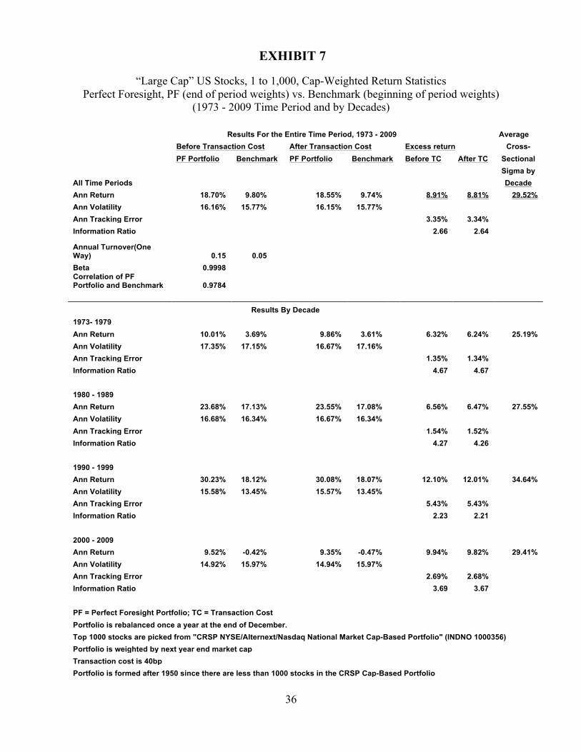
Recall from Exhibit 1 that, after transaction costs, the “perfect foresight” portfolio

averaged an excess return relative to the ex ante Market Portfolio for the large-cap US stocks of

7.19% (bottom of column 6). In Exhibit 7, for the shorter time period 1973 – 2009, our estimate

of the average annual “excess return” is 8.81% after transaction costs (top of column 6). This is

consistent with the increase in the average the cross-sectional dispersion of individual stock

returns (29.52%) for the period 1973 – 2009 (last column in Exhibit 6), compared to 26.72% for

the 1951 – 2009 period (last column, in Exhibit 1). This more than offsets the higher market

return in the longer period of 10.61% (column 4 Exhibit 1) compared to the lower return in the

shorter period, 9.74% (column 4 Exhibit 7.)19 This is consistent with equation (2) in the previous

section and the proof in Appendix A, equation A7.

(Place Exhibit 7 Here}

Moving to the large-cap EAFE stocks, row 2 in Exhibit 8, we see that the results are

similar to the large-cap US segment in Exhibit 6. However, there is more cross-sectional

dispersion of the returns for the individual EAFE stocks (32.33%) and the corresponding

estimated average ex post “excess return” of the PF portfolio for large-cap EAFE segment is also

higher at 9.36%, compared to 8.81% for the large-cap US segment over the same 1973-2009

period. While it is not reported in Exhibits 7 or 8, it is the case that the average large-cap US

stock (the top 1,000) has a slightly greater market value than the average large-cap EAFE stock

over this time period.

{Place Exhibit 8 Here}

19 While it is possible that a higher market return, which is part of the first term on the RHS of equation (2), (1/1+Rm,1) could more than offset an increase the in cross-sectional dispersion of returns, empirically this was never the case during the 51 years of our longer study – see Exhibit 1 and it seems unlikely to us that this will occur in the future.

27

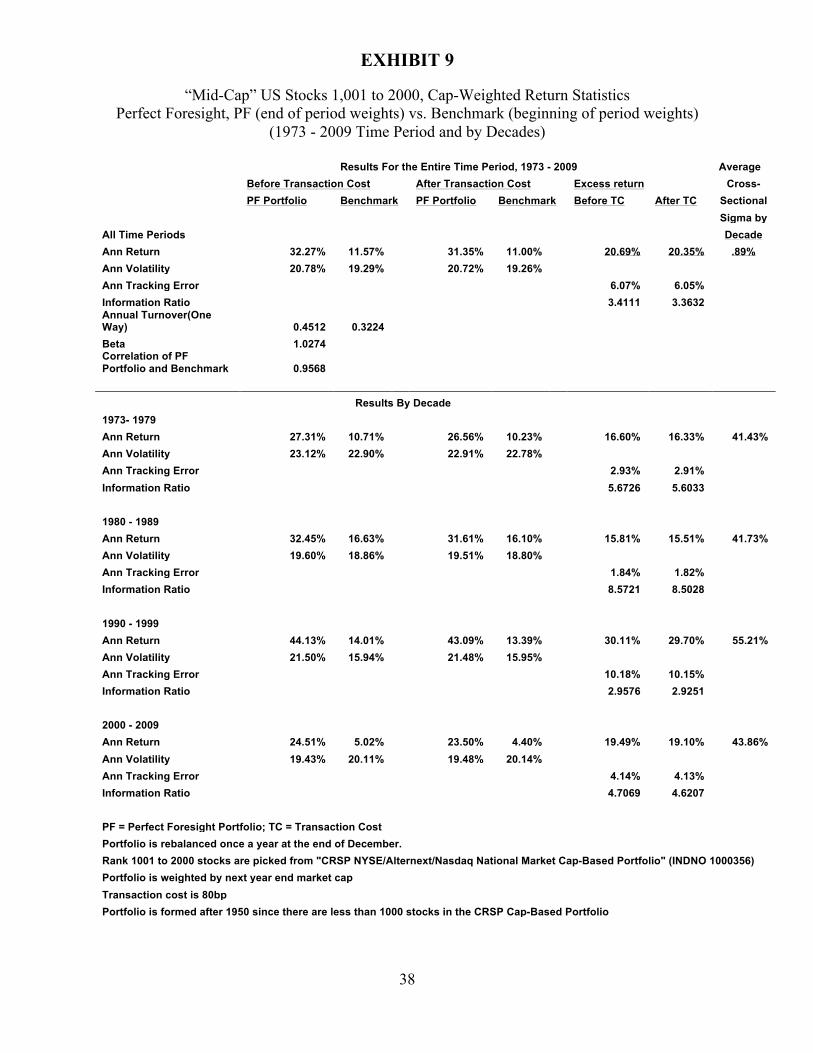
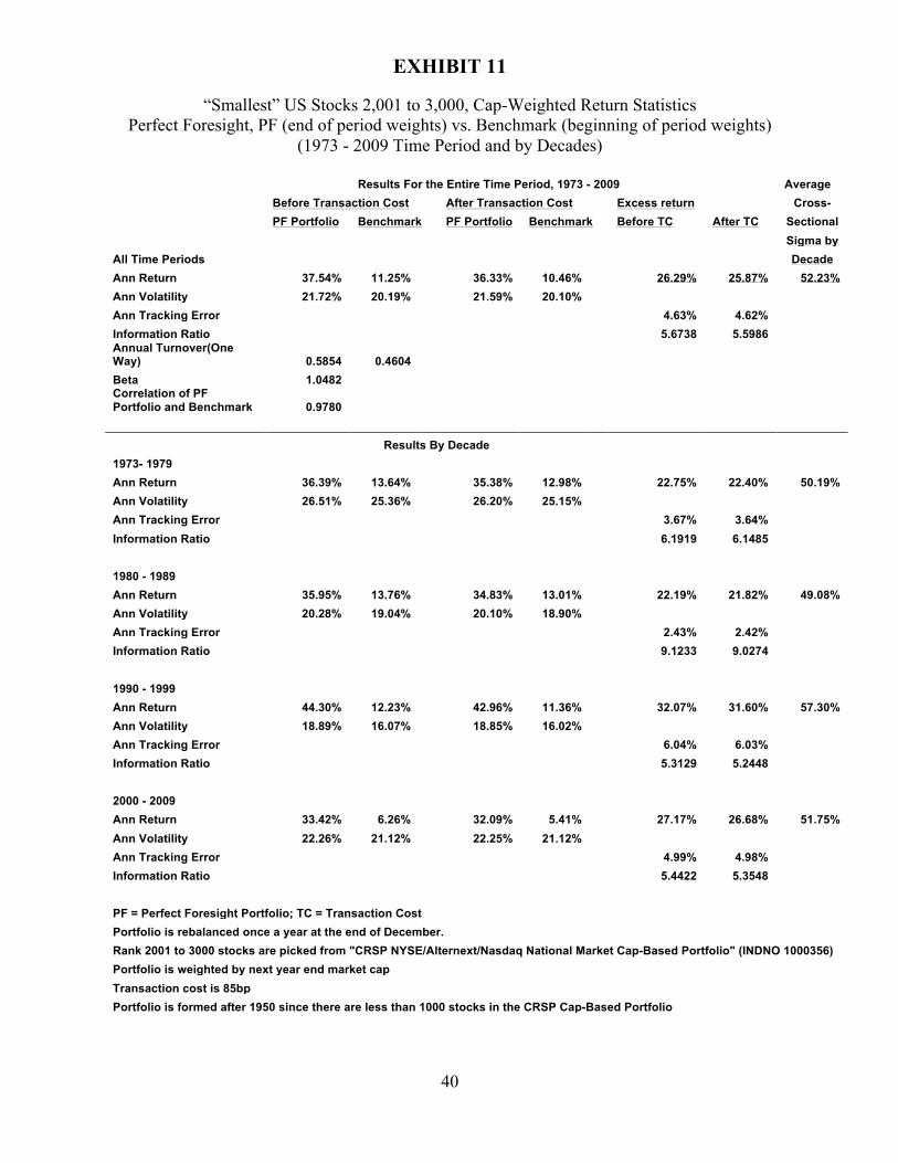
Exhibits 9, 10, and 11 clearly illustrate that as the equity segments move down in terms

of market-cap, the cross-sectional dispersion of the individual stock returns within the segments

increases and the estimated ex post excess return for the ex ante market portfolio increases for

each segment.

{Place Exhibits 9, 10, & 11 Here}

28

REFERENCES

Arnott, Robert D., Feifei Li and Katrina F. Sherrerd (2009), “Clairvoyant Value and the Value Effect,” Journal of Portfolio Management (Spring). Barras, Laurent, Olivier Sacaillet and Russ Wermers (2010), “False Discoveries in Mutual Fund Performance: Measuring Luck in Estimated Alphas,” Journal of Finance (February). Black, Fischer (1988), “Noise,” Journal of Finance (July). Chan, L. K. C.; H. Chen; and J. Lakonishok (2002), “On Mutual Fund Investment Styles. Review of Financial Studies, vol. 15, 1407-1437. Cohen, Randolph, Paul Gompers, and Tuomo Vuolteenaho (2002), “Who underreacts to cash-flow news? Evidence from trading between individuals and institutions,” Journal of Financial Economics, vol. 66, 409-462. De Long, Brad, Andrei Shleifer, Lawrence Summers and Robert Waldmann (1990), “Noise Trader Risk in Financial Markets,” Journal of Political Economy, vol. 98, no.4. Fama, Eugene (1970), “Efficient Capital Markets: A Review of Theory and Empirical Work,” Journal of Finance, vol. 25, 383 - 417. Fama, Eugene (1991), “Efficient Capital Markets: II,” Journal of Finance, 46(2), 1575 - 1617. Fuller, Russell, Bing Han and Yining Tung (2010), “Thinking About Indexes and “Passive vs. Active Management,” Journal of Portfolio Management (Summer). Lakonishok, Josef, Andrei Shleifer, and Robert Vishny (1997), “What do Money Managers Do?” Working Paper, Harvard Business School. LeRoy, Stephen and Charles LaCivita (1981), “Risk Aversion and the Dispersion of Asset Prices,” Journal of Business (October). Markowitz, Harry (2005), “Market Efficiency: A Theoretical Distinction and So What?,” Financial Analyst Journal (September/October). Roll, Richard (1977), “A Critique of the Asset Pricing Theory’s Tests,” Journal of Financial Economics (March). Sharpe, William (1970), Portfolio Theory and Capital Markets, McGraw-Hill. New York. Sharpe, William (2010), “Adaptive Asset Allocation Policy,” Financial Analyst Journal (May/June). Shiller, Robert J. (1979), “The Volatility of Long-Term Interest Rates and Expectation Models of the Term Structure,” Journal of Political Economy (December).

29

Shiller, Robert J. (1981), “Do Stock Prices Move Too Much to Be Justified by Subsequent Changes in Dividends?” American Economic Review (June). Statman, Meir (2011), “Efficient Markets in Crisis,” Journal of Investment Management, vol. 9 (2).

30

FIGURE 1:

Negative Impact of Noise on Cap-Weighted Portfolio Ex Ante: Efficient Frontier

Ex post: Efficient Frontier (Period t = 0,1)

Rm,1

Rp,1

σm,1

σp,1

RPF,1

Negative Effect of Noise on Cap-Weighted Portfolio

Rf

E(Rm,0)

E(Rp,0)

E(σm,0)

E(σp,0)

Rf

31

EXHIBIT 1 Year-by-Year Returns Over Entire Period, 1951 - 2009

Perfect Foresight (end of period weights) vs. Ex Ante (beginning of period weights)

PForesight Portfolio(RPFs,1) Benchmark(Ex Ante) Portfolio (RMs,1) Excess returns Cross-Sectional

Standard Deviation Before TC After TC Before TC After TC Before TC After TC

1951 23.97% 23.50% 20.64% 20.18% 3.33% 3.32% 20.14% 1952 15.45% 15.36% 13.48% 13.45% 1.98% 1.92% 15.60% 1953 2.96% 2.90% 0.66% 0.64% 2.30% 2.26% 14.66% 1954 55.15% 55.04% 49.99% 49.96% 5.17% 5.08% 28.43% 1955 29.03% 28.94% 25.24% 25.22% 3.78% 3.73% 21.51% 1956 11.96% 11.87% 8.33% 8.31% 3.63% 3.56% 19.56% 1957 -6.04% -6.14% -9.96% -9.97% 3.91% 3.83% 18.60% 1958 49.24% 49.11% 44.85% 44.82% 4.40% 4.30% 25.45% 1959 17.20% 17.12% 12.65% 12.63% 4.55% 4.49% 21.91% 1960 7.70% 7.57% 1.17% 1.15% 6.53% 6.42% 25.19% 1961 31.44% 31.33% 27.07% 27.05% 4.37% 4.28% 23.27% 1962 -6.25% -6.33% -9.60% -9.62% 3.35% 3.28% 17.98% 1963 24.10% 23.99% 21.16% 21.11% 2.94% 2.88% 18.68% 1964 18.60% 18.53% 16.12% 16.10% 2.48% 2.43% 17.18% 1965 19.84% 19.73% 13.65% 13.63% 6.19% 6.11% 25.93% 1966 -4.65% -4.74% -8.72% -8.74% 4.07% 4.00% 18.74% 1967 36.37% 36.23% 26.13% 26.11% 10.24% 10.13% 34.21% 1968 17.56% 17.42% 12.45% 12.41% 5.11% 5.00% 23.12% 1969 -3.67% -3.79% -9.84% -9.88% 6.17% 6.09% 23.09% 1970 5.84% 5.70% 1.14% 1.10% 4.70% 4.60% 22.35% 1971 21.97% 21.84% 16.10% 16.06% 5.87% 5.78% 25.14% 1972 22.72% 22.61% 17.85% 17.82% 4.86% 4.79% 23.62% 1973 -8.07% -8.17% -17.09% -17.12% 9.03% 8.95% 27.30% 1974 -21.65% -21.75% -26.99% -27.00% 5.34% 5.25% 20.01% 1975 46.48% 46.32% 37.97% 37.95% 8.51% 8.37% 34.50% 1976 30.61% 30.49% 25.85% 25.82% 4.76% 4.67% 24.79% 1977 -2.38% -2.45% -5.35% -5.37% 2.97% 2.92% 16.51% 1978 10.46% 10.37% 6.89% 6.86% 3.57% 3.51% 19.21% 1979 31.24% 31.11% 21.21% 21.18% 10.03% 9.93% 34.02% 1980 43.52% 43.38% 32.14% 32.11% 11.38% 11.28% 37.71% 1981 3.00% 2.82% -3.91% -3.95% 6.91% 6.77% 25.76% 1982 32.75% 32.60% 20.63% 20.59% 12.12% 12.01% 37.41% 1983 26.98% 26.82% 22.17% 22.11% 4.81% 4.71% 23.92% 1984 9.51% 9.39% 5.52% 5.47% 3.99% 3.92% 22.41% 1985 37.28% 37.14% 32.38% 32.30% 4.91% 4.84% 24.78% 1986 22.95% 22.83% 17.84% 17.79% 5.11% 5.04% 25.96% 1987 9.11% 9.01% 3.29% 3.25% 5.82% 5.76% 24.51% 1988 21.78% 21.64% 17.29% 17.26% 4.48% 4.39% 24.13% 1989 36.90% 36.77% 30.21% 30.17% 6.69% 6.59% 28.87% 1990 1.72% 1.61% -4.46% -4.50% 6.18% 6.11% 23.73% 1991 45.16% 45.01% 33.21% 33.18% 11.95% 11.83% 38.43% 1992 14.59% 14.44% 8.48% 8.44% 6.11% 6.00% 24.79% 1993 16.93% 16.82% 10.31% 10.27% 6.62% 6.55% 26.80% 1994 4.25% 4.13% 0.49% 0.46% 3.76% 3.68% 19.55% 1995 43.20% 43.07% 37.59% 37.54% 5.61% 5.53% 27.32% 1996 29.00% 28.87% 22.31% 22.25% 6.69% 6.62% 27.26% 1997 39.70% 39.55% 32.30% 32.23% 7.40% 7.32% 31.09% 1998 48.88% 48.69% 27.89% 27.82% 20.99% 20.87% 50.75% 1999 77.04% 76.78% 21.37% 21.31% 55.67% 55.47% 76.72% 2000 12.96% 12.60% -9.41% -9.49% 22.37% 22.10% 45.11% 2001 -0.19% -0.37% -12.19% -12.24% 12.00% 11.87% 32.44% 2002 -13.73% -13.84% -21.10% -21.14% 7.37% 7.30% 23.96% 2003 36.31% 36.13% 29.37% 29.33% 6.94% 6.80% 29.17% 2004 16.37% 16.25% 10.99% 10.96% 5.38% 5.29% 23.37% 2005 11.85% 11.75% 6.05% 6.01% 5.80% 5.74% 23.14% 2006 19.41% 19.30% 15.58% 15.55% 3.83% 3.75% 21.01% 2007 17.85% 17.72% 6.53% 6.49% 11.32% 11.22% 33.22% 2008 -26.22% -26.35% -36.09% -36.12% 9.87% 9.77% 25.40% 2009 38.51% 38.24% 27.42% 27.36% 11.08% 10.87% 37.26%

Volatility 14.82% 14.56% High 55.47% 76.72% Correlation 0.9827 Low 1.92% 14.66% Beta 0.9992 Average 7.32% 26.72% Ann. Return 17.80% 10.61% 7.19% Correlation: Excess return After TC & Cross-Sectional Sigma = 93.65%

32

EXHIBIT 2

Time Series Plot of “Perfect Foresight” Excess returns, Net of Transaction Costs,

“Perfect Foresight Weights” vs. Traditional Cap-Weights (1951 – 2009)

Annual Excess Return: RPFs,1 - RMs,1

(Estimated Annual "Mis-Pricing" of the Ex Ante Market Portfolio)

0.00%

10.00%

20.00%

30.00%

40.00%

50.00%

60.00%

195119531955195719591961196319651967196919711973197519771979198119831985198719891991199319951997199920012003200520072009

33

EXHIBIT 3

”Perfect Foresight” Excess Returns (RPFs,1 – RMs,1) and Average Cross-Sectional Standard Deviation of Returns

(By Decade)

PF Portfolio

Excess return Average Cross-

Sectional Before TC After TC Sigma of Returns by Decade 1950s 3.64% 3.58% 20.65% 1960s 5.12% 5.04% 22.74% 1970s 5.98% 5.90% 24.74% 1980s 6.56% 6.47% 27.55% 1990s 12.10% 12.01% 34.64% 2000s 9.94% 9.82% 29.41%

EXHIBIT 4

Plot of “perfect Foresight” Excess returns and Cross-Sectional Sigma of Returns (By Decade)

0.00%

5.00%

10.00%

15.00%

20.00%

25.00%

30.00%

35.00%

40.00%

1950s 1960s 1970s 1980s 1990s 2000s

Excess Return Cross-Sectional Sigma

Correlation of Annual Excess returns vs. Cross-sectional Deviation of Annual Returns = 0.9365

34

EXHIBIT 5

Plot of Estimated Mispricing (“Perfect Foresight” Excess returns) And the Cross-Sectional Sigma of Returns

(Annual Time Series, 1951 - 2009)

Excess Return and Cross-Sectional Sigma of Returns

0.00%

10.00%

20.00%

30.00%

40.00%

50.00%

60.00%

70.00%

80.00%

90.00%

1951

1953

1955

1957

1959

1961

1963

1965

1967

1969

1971

1973

1975

1977

1979

1981

1983

1985

1987

1989

1991

1993

1995

1997

1999

2001

2003

2005

2007

2009

Excess Returns After TCCross-Sectional Standard Deviation

35

EXHIBIT 6

Summary Statistics for Various Equity Market Segments 1973 - 2009

PF Excess return Cross-Sectional

Standard Deviation

Beta Correlation of PF Portfolio and Benchmark

1-1000 8.81% 29.52% 0.9998 0.9784 EAFE 9.36% 32.33% 1.0078 0.9877

1001-2000 20.35% 45.89% 1.0274 0.9568 1001-3000 21.97% 47.77% 1.0325 0.9647 2001-3000 25.87% 52.23% 1.0482 0.9780

1-1000EAFE

1001-2000

1001-3000

2001-3000

0.00%

5.00%

10.00%

15.00%

20.00%

25.00%

30.00%

20.00% 25.00% 30.00% 35.00% 40.00% 45.00% 50.00% 55.00%

Cross-Sectional Standard Deviation

Exce

ss R

etur

n

36

EXHIBIT 7

“Large Cap” US Stocks, 1 to 1,000, Cap-Weighted Return Statistics

Perfect Foresight, PF (end of period weights) vs. Benchmark (beginning of period weights) (1973 - 2009 Time Period and by Decades)

Results For the Entire Time Period, 1973 - 2009 Average Before Transaction Cost After Transaction Cost Excess return Cross- PF Portfolio Benchmark PF Portfolio Benchmark Before TC After TC Sectional Sigma by All Time Periods Decade Ann Return 18.70% 9.80% 18.55% 9.74% 8.91% 8.81% 29.52% Ann Volatility 16.16% 15.77% 16.15% 15.77% Ann Tracking Error 3.35% 3.34% Information Ratio 2.66 2.64

Annual Turnover(One Way) 0.15 0.05 Beta 0.9998 Correlation of PF Portfolio and Benchmark 0.9784 Results By Decade 1973- 1979 Ann Return 10.01% 3.69% 9.86% 3.61% 6.32% 6.24% 25.19% Ann Volatility 17.35% 17.15% 16.67% 17.16% Ann Tracking Error 1.35% 1.34% Information Ratio 4.67 4.67 1980 - 1989 Ann Return 23.68% 17.13% 23.55% 17.08% 6.56% 6.47% 27.55% Ann Volatility 16.68% 16.34% 16.67% 16.34% Ann Tracking Error 1.54% 1.52% Information Ratio 4.27 4.26 1990 - 1999 Ann Return 30.23% 18.12% 30.08% 18.07% 12.10% 12.01% 34.64% Ann Volatility 15.58% 13.45% 15.57% 13.45% Ann Tracking Error 5.43% 5.43% Information Ratio 2.23 2.21 2000 - 2009 Ann Return 9.52% -0.42% 9.35% -0.47% 9.94% 9.82% 29.41% Ann Volatility 14.92% 15.97% 14.94% 15.97% Ann Tracking Error 2.69% 2.68% Information Ratio 3.69 3.67 PF = Perfect Foresight Portfolio; TC = Transaction Cost Portfolio is rebalanced once a year at the end of December. Top 1000 stocks are picked from "CRSP NYSE/Alternext/Nasdaq National Market Cap-Based Portfolio" (INDNO 1000356) Portfolio is weighted by next year end market cap Transaction cost is 40bp Portfolio is formed after 1950 since there are less than 1000 stocks in the CRSP Cap-Based Portfolio

37

EXHIBIT 8

EAFE Large-Cap Stocks, Cap-Weighted Return Statistics

Perfect Foresight, PF (end of period weights) vs. Benchmark (beginning of period weights) (1973 - 2009 Time Period and by Decades)

Results For the Entire Time Period, 1973 - 2009 Average Before Transaction Cost After Transaction Cost Excess return Cross- PF Portfolio Benchmark PF Portfolio Benchmark Before TC After TC Sectional Sigma by All Time Periods Decade Ann Return 19.56% 9.95% 19.18% 9.82% 9.61% 9.36% 32.33% Ann Volatility 17.79% 17.39% 17.79% 17.40% Ann Tracking Error 2.82% 2.79% Information Ratio 3.4102 3.3575 Annual Turnover(One Way) 0.2020 0.0574 Beta 1.0078 Correlation of PF Portfolio and Benchmark 0.9877 Results By Decade 1973- 1979 Ann Return 17.50% 7.52% 17.07% 7.33% 9.99% 9.74% 33.05% Ann Volatility 17.68% 16.84% 17.60% 16.82% Ann Tracking Error 2.43% 2.36% Information Ratio 4.1056 4.1312 1980 - 1989 Ann Return 34.42% 23.00% 34.00% 22.88% 11.42% 11.12% 38.57% Ann Volatility 18.88% 17.47% 18.85% 17.46% Ann Tracking Error 3.24% 3.20% Information Ratio 3.5262 3.4773 1990 - 1999 Ann Return 17.59% 7.94% 17.28% 7.84% 9.65% 9.43% 31.01% Ann Volatility 17.19% 17.23% 17.18% 17.23% Ann Tracking Error 3.21% 3.19% Information Ratio 3.0054 2.9557 2000 - 2009 Ann Return 9.44% 1.69% 9.09% 1.57% 7.75% 7.52% 26.92% Ann Volatility 17.01% 17.61% 17.09% 17.64% Ann Tracking Error 2.10% 2.11% Information Ratio 3.6840 3.5598 PF = Perfect Foresight Portfolio; TC = Transaction Cost Portfolio is rebalanced once a year at the end of December. Portfolio is weighted by next year end market cap Transaction cost is 85bp

38

EXHIBIT 9

“Mid-Cap” US Stocks 1,001 to 2000, Cap-Weighted Return Statistics Perfect Foresight, PF (end of period weights) vs. Benchmark (beginning of period weights)

(1973 - 2009 Time Period and by Decades) Results For the Entire Time Period, 1973 - 2009 Average Before Transaction Cost After Transaction Cost Excess return Cross- PF Portfolio Benchmark PF Portfolio Benchmark Before TC After TC Sectional Sigma by All Time Periods Decade Ann Return 32.27% 11.57% 31.35% 11.00% 20.69% 20.35% .89% Ann Volatility 20.78% 19.29% 20.72% 19.26% Ann Tracking Error 6.07% 6.05% Information Ratio 3.4111 3.3632 Annual Turnover(One Way) 0.4512 0.3224 Beta 1.0274 Correlation of PF Portfolio and Benchmark 0.9568 Results By Decade 1973- 1979 Ann Return 27.31% 10.71% 26.56% 10.23% 16.60% 16.33% 41.43% Ann Volatility 23.12% 22.90% 22.91% 22.78% Ann Tracking Error 2.93% 2.91% Information Ratio 5.6726 5.6033 1980 - 1989 Ann Return 32.45% 16.63% 31.61% 16.10% 15.81% 15.51% 41.73% Ann Volatility 19.60% 18.86% 19.51% 18.80% Ann Tracking Error 1.84% 1.82% Information Ratio 8.5721 8.5028 1990 - 1999 Ann Return 44.13% 14.01% 43.09% 13.39% 30.11% 29.70% 55.21% Ann Volatility 21.50% 15.94% 21.48% 15.95% Ann Tracking Error 10.18% 10.15% Information Ratio 2.9576 2.9251 2000 - 2009 Ann Return 24.51% 5.02% 23.50% 4.40% 19.49% 19.10% 43.86% Ann Volatility 19.43% 20.11% 19.48% 20.14% Ann Tracking Error 4.14% 4.13% Information Ratio 4.7069 4.6207 PF = Perfect Foresight Portfolio; TC = Transaction Cost Portfolio is rebalanced once a year at the end of December. Rank 1001 to 2000 stocks are picked from "CRSP NYSE/Alternext/Nasdaq National Market Cap-Based Portfolio" (INDNO 1000356) Portfolio is weighted by next year end market cap Transaction cost is 80bp Portfolio is formed after 1950 since there are less than 1000 stocks in the CRSP Cap-Based Portfolio

39

EXHIBIT 10

“R2000”, US Stocks 1,001 to 3,000, Cap-Weighted Return Statistics Perfect Foresight, PF (end of period weights) vs. Benchmark (beginning of period weights)

(1973 - 2009 Time Period and by Decades) Results For the Entire Time Period, 1973 - 2009 Average Before Transaction Cost After Transaction Cost Excess return Cross- PF Portfolio Benchmark PF Portfolio Benchmark Before TC After TC Sectional Sigma by All Time Periods Decade Ann Return 33.84% 11.49% 33.04% 11.06% 22.35% 21.97% 47.77% Ann Volatility 20.88% 19.43% 20.82% 19.41% Ann Tracking Error 5.54% 5.53% Information Ratio 4.0305 3.9761 Annual Turnover(One Way) 0.3878 0.2366 Beta 1.0325 Correlation of PF Portfolio and benchmark 0.9647 Results By Decade 1973- 1979 Ann Return 29.73% 11.44% 29.05% 11.06% 18.28% 17.99% 43.88% Ann Volatility 23.92% 23.46% 23.74% 23.38% Ann Tracking Error 3.00% 2.98% Information Ratio 6.0991 6.0444 1980 - 1989 Ann Return 33.43% 15.88% 32.71% 15.49% 17.55% 17.22% 43.83% Ann Volatility 19.70% 18.84% 19.62% 18.78% Ann Tracking Error 1.90% 1.88% Information Ratio 9.2268 9.1479 1990 - 1999 Ann Return 44.41% 13.54% 43.52% 13.07% 30.87% 30.44% 55.94% Ann Volatility 20.59% 15.88% 20.57% 15.87% Ann Tracking Error 9.04% 9.01% Information Ratio 3.4148 3.3786 2000 - 2009 Ann Return 27.17% 5.36% 26.29% 4.91% 21.81% 21.37% 46.26% Ann Volatility 20.09% 20.28% 20.12% 20.30% Ann Tracking Error 4.14% 4.13% Information Ratio 5.2727 5.1791 PF = Perfect Foresight Portfolio; TC = Transaction Cost Portfolio is rebalanced once a year at the end of December. Rank 1001 to 3000 stocks are picked from "CRSP NYSE/Alternext/Nasdaq National Market Cap-Based Portfolio" (INDNO 1000356) Portfolio is weighted by next year end market cap Transaction cost is 80bp Portfolio is formed after 1950 since there are less than 1000 stocks in the CRSP Cap-Based Portfolio

40

EXHIBIT 11

“Smallest” US Stocks 2,001 to 3,000, Cap-Weighted Return Statistics Perfect Foresight, PF (end of period weights) vs. Benchmark (beginning of period weights)

(1973 - 2009 Time Period and by Decades) Results For the Entire Time Period, 1973 - 2009 Average Before Transaction Cost After Transaction Cost Excess return Cross- PF Portfolio Benchmark PF Portfolio Benchmark Before TC After TC Sectional Sigma by All Time Periods Decade Ann Return 37.54% 11.25% 36.33% 10.46% 26.29% 25.87% 52.23% Ann Volatility 21.72% 20.19% 21.59% 20.10% Ann Tracking Error 4.63% 4.62% Information Ratio 5.6738 5.5986 Annual Turnover(One Way) 0.5854 0.4604 Beta 1.0482 Correlation of PF Portfolio and Benchmark 0.9780 Results By Decade 1973- 1979 Ann Return 36.39% 13.64% 35.38% 12.98% 22.75% 22.40% 50.19% Ann Volatility 26.51% 25.36% 26.20% 25.15% Ann Tracking Error 3.67% 3.64% Information Ratio 6.1919 6.1485 1980 - 1989 Ann Return 35.95% 13.76% 34.83% 13.01% 22.19% 21.82% 49.08% Ann Volatility 20.28% 19.04% 20.10% 18.90% Ann Tracking Error 2.43% 2.42% Information Ratio 9.1233 9.0274 1990 - 1999 Ann Return 44.30% 12.23% 42.96% 11.36% 32.07% 31.60% 57.30% Ann Volatility 18.89% 16.07% 18.85% 16.02% Ann Tracking Error 6.04% 6.03% Information Ratio 5.3129 5.2448 2000 - 2009 Ann Return 33.42% 6.26% 32.09% 5.41% 27.17% 26.68% 51.75% Ann Volatility 22.26% 21.12% 22.25% 21.12% Ann Tracking Error 4.99% 4.98% Information Ratio 5.4422 5.3548 PF = Perfect Foresight Portfolio; TC = Transaction Cost Portfolio is rebalanced once a year at the end of December. Rank 2001 to 3000 stocks are picked from "CRSP NYSE/Alternext/Nasdaq National Market Cap-Based Portfolio" (INDNO 1000356) Portfolio is weighted by next year end market cap Transaction cost is 85bp Portfolio is formed after 1950 since there are less than 1000 stocks in the CRSP Cap-Based Portfolio