Embed Size (px)
Citation preview

Applied Energy 115 (2014) 190–204
Contents lists available at ScienceDirect
Applied Energy
journal homepage: www.elsevier .com/ locate/apenergy
Estimating the potential of controlled plug-in hybrid electric vehiclecharging to reduce operational and capacity expansion costs for electricpower systems with high wind penetration
0306-2619/$ - see front matter � 2013 Elsevier Ltd. All rights reserved.http://dx.doi.org/10.1016/j.apenergy.2013.10.017
⇑ Corresponding author. Address: Carnegie Mellon University, EPP Baker 129,5000 Forbes Ave, Pittsburgh, PA 15213, United States. Tel.: +1 (412)973 6185.
E-mail address: [email protected] (A. Weis).
Allison Weis ⇑, Paulina Jaramillo, Jeremy MichalekCarnegie Mellon University, United States
h i g h l i g h t s
�We quantify the benefits of controlled charging of plug-in hybrid electric vehicles.� Costs are determined using an economic dispatch and unit commitment model.� The model is based on New York ISO and allows for capacity expansion.� We find controlled charging can significantly lower system costs.� Controlled charging benefits are larger with high wind penetration.
a r t i c l e i n f o
Article history:Received 25 April 2013Received in revised form 3 September 2013Accepted 7 October 2013
Keywords:DispatchCapacity expansionPlug-in hybrid electric vehiclesControlled chargingWind power integration
a b s t r a c t
Electric power systems with substantial wind capacity require additional flexibility to react to rapidchanges in wind farm output and mismatches in the timing of generation and demand. Controlled vari-able-rate charging of plug-in electric vehicles allows demand to be rapidly modulated, providing an alter-native to using fast-responding natural gas plants for balancing supply with demand and potentiallyreducing costs of operation and new plant construction. We investigate the cost savings from controlledcharging of electric vehicles, the extent to which these benefits increase in high wind penetration scenar-ios, and the trade-off between establishing a controlled charging program vs. increasing the capacity ofgenerators in the power system. We construct a mixed integer linear programming model for capacityexpansion, plant dispatch, and plug-in hybrid electric vehicle (PHEV) charging based on the NYISO sys-tem. We find that controlled charging cuts the cost of integrating PHEVs in half. The magnitude of thesesavings is �5% to 15% higher in a system with 20% wind penetration compared to a system with no windpower, and the savings are 50–60% higher in a system that requires capacity expansion.
� 2013 Elsevier Ltd. All rights reserved.
1. Introduction
Electricity generation is responsible for over 40% of US CO2
emissions [1], and producing electricity from traditional fossil fuelsources also creates other emissions that harm human health andthe environment, such as NOx and SO2. Integrating low-emissionpower options, such as wind and solar power, will play a key rolein reducing harmful emissions. Many states have recognized theneed for more renewable energy production, and twenty-ninestates have adopted renewable energy portfolio standards (RPS)requiring between 10% and 40% of generated power to come from
renewable sources [2]. As one of the fastest growing electricitysources in the United States [3], wind can be expected to meet alarge proportion of the renewable portfolio standards. To compen-sate for the increased amounts of these inherently–variablesources of electricity, the power grid requires additional flexibilityto manage fluctuations in generation. For systems incorporatinghigh levels of wind power, ramping natural gas combustion turbineplants in response to changes in output from variable resources hastypically provided this flexibility. Recent research has shown thatramping gas turbines to manage the variability of wind powercan increase NOx emissions and reduce the greenhouse gas bene-fits associated with wind power production [4].
Plug-in electric vehicles (PEVs), including plug-in hybrid elec-tric vehicles (PHEVs) and battery electric vehicles (BEVs), createadditional electricity demand, resulting in additional air emissionsfrom power plants [5,6]. But they have also been proposed as a

A. Weis et al. / Applied Energy 115 (2014) 190–204 191
means for increasing grid flexibility in order to integrate renew-ables, with much emphasis on the possibility of using the vehiclesfor grid storage via a bidirectional electrical connection betweenthe vehicle and the electricity grid, referred to as vehicle-to-grid(V2G). For example, Lund and Kempton calculate the cost-savingsand emissions-savings from adding V2G capabilities to the powersystem, given simplified ramping constraints for the power gener-ation fleet [7]. However, it has been shown that the market for V2Gin the energy market [8] and ancillary services market [9] is small,arbitrage potential is limited, and participation can significantly re-duce battery life by increasing the total energy processed by thebattery [9]. V2G systems also require a substantial investment inpower electronics, control software, and additional grid infrastruc-ture. As an alternative, electricity demand can be partially man-aged by modulating the charging rate of PEVs – for example,following variations in wind supply. Such an approach does not in-crease the energy processed by the battery, and it is possible thatsuch an approach could actually extend battery life by loweringaverage charge rates and thus heat generation [10]. Controlledcharging can also take advantage of the high levels of wind gener-ation that commonly occur at night in the US. At these times otherload is likely to be low, and coal plants would likely need to becycled, adding costs and emissions that could be saved with smartcharging of PEVs. Alternatively, ramping of thermal plants could bereduced by building excess wind capacity, curtailing wind energywhen it is not needed, and taking it when most cost effective forthe system.
Previous work has shown the benefit of controlled charging inpower systems with wind power. Dallinger et al. show that excessrenewable energy in periods of low load can be significantly re-duced through optimized charging in California and Germany[11], and Foley et al. find that off-peak charging can save vehicleowners nearly 30% of the charging costs [12]. Wang et al. evaluatedifferent charging strategies of plug-in hybrid vehicles in the Illi-nois power system and find significant cost savings with controlledcharging. They assume the rest of the power system is static anduse a simple scaling of existing wind data to model new wind con-struction [13], exaggerating variability by ignoring the complex ef-fects of plant size and geographic diversity on mitigating windgeneration correlation [14]. Sioshansi and Denholm analyze a sys-tem based on the Electric Reliability Corporation of Texas (ERCOT)in its current form, with 10% wind generation, to calculate theadditional benefit of V2G over controlled charging, again allowingonly operation of existing power plants to vary [15]. They find thatV2G could decrease system costs by around 0.5%. Instead of hold-ing existing capacity fixed as in these studies, we consider a case inwhich new capacity needs to be built to meet required system re-serve margins. As discussed by De Jonge et al. it is important toconsider the capacity expansion in the context of all the opera-tional constraints of the power plants [16].
Other work has focused on how controlled charging can beused as balancing power in systems with high wind penetrationby modeling forecasting error for wind and load instead of eval-uating detailed operating constraints. A study by the PacificNorthwest National Laboratory estimates the number of vehiclesnecessary to provide a complete response to the balancing signal[17], capturing the high frequency behavior of the wind andvehicle charging but ignoring other types of flexibility alreadypresent in the grid. Druitt and Früh also focus on how controlledelectric vehicle charging can provide balancing power at highwind penetrations [18]. They use a simplified scheduling of con-ventional generation, which ignores many operating constraints,and develop a model based on historic prices to estimate eco-nomic effects.
We seek to evaluate the potential cost savings from controlledcharging in scenarios with vs. without additional wind power in
order to understand whether PEVs can provide cost savings insystems with increased levels of wind power, or whether con-trolled charging only limits the impact of the vehicles themselveson the system. We focus on PHEVs, which do not require changesin current driving patterns, since PHEVs can operate using gasolinefor long trips. The interaction of PHEV charging with the grid iscomplex, and a complete understanding requires evaluating thepower system in a range of circumstances and at a variety of timescales. We examine the benefit of controlled charging of PHEVs rel-ative to convenience charging (vehicle charges at maximum rateupon arrival), delayed charging (vehicle begins charging at maxi-mum rate just in time for its next use), and no charging (no PHEVs)under alternative scenarios of high vs. low wind penetration in thepower generation fleet, high vs. low PHEV penetration in the vehi-cle fleet, and high vs. low initial power generating capacity. For thisanalysis, we develop a capacity expansion and unit commitmentwith economic dispatch optimization model with detailed plantconstraints. We use hourly data for wind and load and assume per-fect information (no forecast error) to focus on capacity expansionand unit commitment decisions. We then compare results using a15-min resolution to test the importance of sub-hourly trends. Westudy a period of 20 days selected to be representative of the year.We do not evaluate the entire range of power plant fleets that existin the US but instead focus on comparing the difference between asystem with sufficient capacity and one requiring investment innew capacity.
In the remaining sections we present our detailed methods, re-sults, and conclusions. We find that controlled charging does helpto reduce system costs by about 2% in the scenarios examined with10% PHEV penetration. However, the additional benefit of con-trolled charging in high wind-penetration scenarios is much smal-ler. Thus the benefits of controlled charging are general to powersystems and not specific to wind integration under the scenariosexamined. We also examine the tradeoff between adding newcapacity to the system versus controlled charging in order toaccommodate high wind penetration scenarios, finding that con-trolled charging reduces the number of combined cycle gas plantsthat would otherwise be built.
2. Methods
2.1. Model overview
We pose a mixed integer linear programming (MILP) capacityexpansion model with hourly unit commitment and dispatch,plus hourly vehicle availability and charging rates, to find theoptimal combination of new power plants and controlled vehiclecharging to meet demand at lowest costs subject to operationconstraints. Capacity expansion optimizes which power plantsshould be added to the system, if any. Unit commitment and dis-patch determine which plants will be on in each time period andthe level of output for each. As part of the cost minimization, themodel also determines the charge rate in each hour for each setof available vehicles, where the set of vehicle driving profilesare selected to be representative of the US vehicle population.The model treats the penetration of plug-in vehicles that mustbe charged as exogenous, and the grid operator can choose a per-centage of the vehicles to participate in a controlled charging pro-gram for a given annual payment. We vary the number ofvehicles present in the system and the amount of the annual pay-ment to vehicle owners in a sensitivity analysis. The model con-strains electricity generation to match the load in each timestep, while keeping all plants within their operating constraintsand satisfying a wind penetration goal that defines a minimumpercentage of overall power generation that must be supplied

Fig. 1. System overview – energy is provided by conventional power plants andwind plants and must meet the demand from plug-in vehicles and non-vehicle loadin each time step.
0
5
10
15
20
25
30
35
40
45
Actual Capacity Capacity Expansion Fixed Capacity
Inst
alle
d C
apac
ity
(GW
)
Other
Hydro
Oil/Gas Steam
Gas Turbine
Combined Cycle
Coal
Nuclear
Fig. 2. Installed capacity of the actual capacity of the NYISO power plant fleet,Capacity Expansion Scenario, and the Fixed Capacity Scenario.
192 A. Weis et al. / Applied Energy 115 (2014) 190–204
by wind1,2. Fig. 1 shows a graphical representation of the frame-work used.
2.2. Power plant fleets
We construct two different power plant fleet scenarios usingpower plant fleet characteristics from the New York IndependentSystem Operator (NYISO) area: the first scenario with sufficientexisting capacity to meet vehicle and non-vehicle load (FixedCapacity Scenario); and the second where capacity expansion is re-quired regardless of PHEV penetration (Capacity Expansion Sce-nario). Because NYISO has significant amounts of hydroelectricpower for which operational data is unavailable, we constructthe Capacity Expansion Scenario by eliminating the hydro capacityfrom NYISO and using only existing nuclear, coal, oil, and naturalgas capacity as the initial state of the fleet. For the Fixed CapacityScenario we replace the hydro capacity with fossil fuel plantsroughly proportional to the existing fossil fuel mix. Individualplant data were not available for all fossil fuel plants in NYISO,so the fleet was chosen from a sample of similar plants in NYISO,ERCOT and PJM with available data. The plants were selected usingan optimization that minimizes the difference between actual fleetcharacteristics and the selected fleet characteristics.
minimizeX
sKTOT
s � xTOTs
��� ���þw1
Xs
Xc2Cs
KBINsc � xCBIN
sc
��� ���þw2
Xs
Xh2Hs
jHsh � xHRBINsh j
where total capacity of plants of each plant types is KTOTs for the actual
fleet and xTOTs for the selected fleet. The number of plants in each
capacity bin c 2 Cs for fuel type s is KBINs for the actual fleet and
xCBINsc for the selected fleet, and similarly the capacity of plants in each
heat rate bin h 2Hs for fuel type s is Hsh for the actual fleet and xHRBINsh
for the selected fleet. The distributions of plant capacities and heatrate were defined using four evenly spaced bins for each plant type.The optimization variables are how many of each of the sample plantsare included in the selected plant fleet and xTOT
s , xCBINsc , and xHRBIN
sh arecalculated from this selected fleet. We found that relative weightsof w1 = 300, and w2 = 100, respectively for these three factors in the
1 As the cheapest renewable energy source by levelized cost, wind is likely to makeup the bulk of power installed to meet RPS. Some RPS policies include specific set-asides for solar power, but these are very small: 0.2–2.5% [2]. For this paper, we modela system in which wind is the only renewable available.
2 The model took between 5–10 h to run on an Intel i& processor running CPLEXusing 20 day period with hourly data. Running the 15-min sensitivity cases over 20days had a wide range of solve times, going up to 80 h for each charging scenario.Because solve time for MILP problems is nonlinear with the number of variables, itwas not feasible to use smaller time steps or more days for all of the sensitivity casesanalyzed.
objective function gave a good fleet representation for these fueltypes. The fuel types that could be modeled in this way for NYISOwere bituminous coal plants, natural gas combined cycle, naturalgas combustion turbine, and oil/gas steam, whereas nuclear wasmodeled as a single capacity and heat rate. The resulting fleets areshown by plant type in Fig. 2. Because of the missing data, the fleetsused in this analysis are not meant to exactly replicate the New Yorksystem, but rather serve as a test system with realistic plant distribu-tions matched to a realistic load. Average ramp rates and minimumgeneration levels by generation type, along with the individual plantheat rates and total capacity for the sample of plants used, were takenfrom Ventyx [19], and the distribution of power plant capacities andheat rates for NYISO were taken from the National Electric EnergyData System (NEEDS) [20]. A comparison of the resulting characteris-tics for the Fixed Capacity Scenario and actual NYISO fleet is shown inTable 1. We are able to obtain a similar fleet according to measurablecharacteristics. The only large difference is the average age of the nat-ural gas combustion turbine plants due to the available data tochoose from. The simulated fleet is newer, but because the averageheat rate remains very close to that of the actual fleet, there shouldnot be a large impact on total operational cost. The newer gas plantsmay be somewhat more flexible, but on the hourly time scale, com-bustion turbine plants have excess ramping capability.’’
2.3. Plug-in hybrid electric vehicle fleet
We model a fleet of plug-in hybrid electric vehicles using theNational Household Travel Survey (NHTS) data set [21], which con-tains data for one day of driving for approximately 900,000 differ-ent passenger cars across the United States. We use time of arrivaland departure from home and distance traveled from all vehicles inthe dataset, weighted by vehicle to be nationally representative, tocompute uncontrolled electricity demand in the conveniencecharging (charge upon arrival at home) and delayed charging(charge just before departure) cases. The controlled-charging sce-narios use 20 representative driving profiles for computationaltractability. Weighted profiles were selected to match the charac-teristics of the overall data set (see Appendix A for more details).The PHEVs we study operate in charge-depleting mode until thebattery reaches its minimum state of charge or all the miles aredriven (sometimes called extended-range electric vehicles (EREVs),like the Chevy Volt). Any remaining miles are driven in charge-sus-taining (extended-range) mode, powered by the gasoline engine3.
3 We do not consider blended-operation PHEVs, like the PHEV Prius, which use alend of gasoline and electricity in charge depleting mode. In our model, whichcuses on electricity consumption, a blended-operation PHEV would function
quivalently to a higher-efficiency EREV PHEV, since the partial use of gasolineffsets some electricity use in charge depleting mode.
bfoeo

Table 1Comparison between the coal, natural gas, and oil/gas steam plants in the actual NYISO fleet and the simulated fleet in terms of capacity installed, number of units, average heatrate, and online year.
Type Actual MW Sim. MW Ref. # units Sim. # units Actual ave HR(BTU/kW h)
Sim. ave HR(BTU/kW h)
Actual aveonline year
Sim. aveonline year
Coal 2767 2767 32 31 10,507 10,738 1970 1962NGCC 8124 8124 103 103 8555 8584 1996 1995NGCT 4885 4885 215 215 14,971 14,945 1976 1992Oil/gas steam 11,723 11,723 32 32 11,341 11,763 1964 1963
A. Weis et al. / Applied Energy 115 (2014) 190–204 193
This allows all drivers to retain their existing driving patterns,regardless of the electric range of the vehicle. The base-case vehicleis modeled after the Chevy Volt with a 16 kW h hour lithium ion bat-tery of which 10.4 kW h are useable. We assume the vehicles onlycharge after their last trip of the day and must be fully charged bytheir first trip of the next day if controlled by the system operatorin the controlled charging program. The charging program altersthe rate of charge for each vehicle but does not withdraw powerfrom the battery. Charging for a portion of a time step is equivalentto charging for the entire time step at a lower rate. We model differ-ent levels of program costs, ranging from $0–$400/vehicle/year.These assumed costs would have to cover both payments to thevehicle owners as well as any infrastructure costs. with the systemoperator determining how many vehicles will be paid for participa-tion (the zero fee case allows the system operator to capture all ofthe cost savings). We perform a sensitivity analysis to examine sup-ply solutions at different participation fee levels and leave as futurework an estimate of the vehicle owner demand curve. We also per-form sensitivity analysis to examine a range of vehicle characteris-tics, shown below in Table 2, as well as different vehiclepenetration levels and payment to vehicle owners. The growth rateof PHEV penetration is very uncertain, but the governor of New Yorkwas quoted as saying ‘‘the number of plug-in electric vehicles on theroad in New York State could increase from less than 3000 today to30,000–40,000 in 2018 and one million in 2025,’’ [22] which wouldbe around 10% of the approximately 9 million passenger vehicles inNew York in 2008 [23]. Additionally, EIA estimates that PHEV’s couldaccount for 2–18% of all vehicles in the US in 2025 depending onwhat policies are adopted [24].
2.4. Wind power data
We use modeled wind production data for all potential land-based wind sites in New York reported in the Eastern Wind Inte-gration and Transmission Study (EWITS) dataset [25]. EWITS listsall the sites in the Eastern Interconnect that would be needed in or-der to reach a 30% RPS and contains ten-minute modeled wind
Table 2Ranges of values used to reflect the uncertainty in the characteristics of the futureplug-in vehicle fleet. The base case for the battery size comes from the Chevy Volt,allowing for roughly 35 miles of driving on electric power, with minimum andmaximum battery sizes allowing for 5 miles and 60 miles of electric driving,respectively. Vehicles with larger and smaller batteries are assumed to have thesame ratio of useable kWh to total kWh as the base case (65%). The range of chargerates come from the three standard levels of electric vehicle charging. Level 1charging can be achieved from a normal household 120 V plug and is used as theminimum. Level 2 charging requires a 240 V outlet, such as those used by largerhousehold appliances, but is more convenient for vehicle owners and is used as thebase case. Level 3 charging requires higher voltage and current levels than typicallyavailable on the household level but is possible at future service stations and is theupper bound on vehicle charge rates. Total fleet size in New York is 9 millionpassenger vehicles, and the range of 1–15% plug-in vehicle penetration represents90,000–1,350,000 plug-in electric vehicles.
Vehicle fleet characteristics Minimum Base case Maximum
Battery size 5 kW h 16 kW h 24 kW hMaximum charging rate 1.2 kW 7.4 kW 30 kWPlug-in vehicle Penetration 1% 10% 15%
plant output for these sites for 3 years from 2006 to 2008. We con-vert the ten-minute power data to hourly resolution for modeltractability by averaging the six data points given for each hour.We then add wind sites from the EWITS data set to our model inorder of highest capacity factor. We investigate wind penetrationrates that range from 0% to 20% to allow for additional wind plantsto be built in all scenarios without making use of offshore wind, asit is uncertain that offshore wind sites will be widely utilized by2025.
We use modeled wind data instead of measured output datafrom existing wind sites so that wind capacity can be expandedbeyond existing levels. Because wind production is dependenton local weather patterns and geography, existing empirical winddata cannot be easily scaled up to include new sites. The EWITSdataset is the only existing public sources for a time series simu-lation of wind production for potential wind sites in this area ofthe country.
2.5. Load data
We use five minute power demand data for the New York ISO in2006, again converted to hourly resolution by averaging the twelvedata points given for each hour. As load is predicted to remainwithin 1% of its current level by 2025 [26], this 2006 data is usedas non-vehicle load without any scaling. It is important to use loadand wind data from the same time and place to account for tempo-ral and geographical correlations. While this paper focus on a mod-el based on the characteristics of the New York System, the methoddeveloped could later be applied to other systems around thecountry. This additional analysis, however, is beyond the scope ofthis paper.
To ensure a reasonable computation time, we chose four differ-ent periods of five days each to capture the different shape of theload curve in different seasons and include the year’s peak load,while keeping the average load over the four periods equal to theaverage load of the year, 19 GW. Six of the 20 days are weekenddays. Given the wind plants needed to meet the 20% penetrationover the course of the entire year (when run as must-take), thewind generation from the modeled wind plants in these four peri-ods is both sufficient to meet the wind penetration goal (scaledwithin the twenty days) without building additional wind plants,and has an average power within 10% of the annual average windpower. Within each of the four periods, plant operating constraintsapply. The model’s capacity expansion variables apply simulta-neously across all four periods, along with the percent of PHEVswith controlled charging.
2.6. Optimization
The optimization model minimizes capital and operating costs:
minimizeX
i2W[NcBLD
i yBLDi|fflfflfflfflfflfflfflfflfflfflfflfflfflffl{zfflfflfflfflfflfflfflfflfflfflfflfflfflffl}
New Plant Construction
þ cEVnEVxEVCTRL|fflfflfflfflfflfflfflffl{zfflfflfflfflfflfflfflffl}
Payments to PHEV Owners
þX
t2T
Xi2C
xSUCit þ xSDC
it þ cFi hixG
it
� �� �|fflfflfflfflfflfflfflfflfflfflfflfflfflfflfflfflfflfflfflfflfflfflfflfflfflfflfflfflfflfflfflfflfflfflffl{zfflfflfflfflfflfflfflfflfflfflfflfflfflfflfflfflfflfflfflfflfflfflfflfflfflfflfflfflfflfflfflfflfflfflffl}
Cost of Plant Operations

194 A. Weis et al. / Applied Energy 115 (2014) 190–204
where N is the set of new conventional power plants; E is the set ofexisting conventional power plants; C ¼N [ E is the combined setof existing and new conventional power plants; W is the set of(new) wind plants; T is the set of time steps in the sample period;cBLD
i is the annualized cost for construction of plant i; yBLDi is the bin-
ary variable determining whether or not plant i is constructed; cEV isthe annual payment to each vehicle owner participating in the con-trolled charging program; nEV is the total number of PHEVs; xEV
CTRL isthe percentage of PHEVs are that are controlled; xSUC
it and xSDCit are
the start-up and shut-down costs, respectively, of plant i in timestep t, cF
i is the fuel cost of plant i, hi is the heat rate of plant i,and xG
it is the power output of the plant i in time step t. We varythe value of the annual payment to each participating vehicle ownerwith a sensitivity analysis to understand the willingness to pay ofthe system operator. The willingness to accept controlled chargingby vehicle owners is unknown and is outside the scope of thispaper.
The constraints are typical for economic unit commitment anddispatch models with plug-in vehicles, but they are adapted to al-low for additional binary variables to represent new power plantconstruction and a variable for the percentage of plug-in vehiclesparticipating in the controlled charging program. The overall sys-tem must meet the existing non-vehicle load plus the vehicle loadof both the controlled and uncontrolled vehicles in every time step:
xWt þ
Xi2C
xGit ¼ Lt þ
Xj2V
xEVjt þ 1� xEV
CTRL
� �nEVmUCTRL
t 8t 2T
where xWt is the amount of wind energy used in time step t, xEV
jt isthe total amount of energy consumed to charge all vehicles of pro-file j in time step t, V is the set of all PHEV profiles, and vUCTRL
t is thefixed amount of uncontrolled charging that occurs for vehicle pro-file j in time step t. The wind penetration goal must be met overthe 20 days:
Xt2T
xWt P ERPS
Xt2T
xWt þ
Xi2C
xGit
! !
where ERPS is the percent wind energy required by the penetrationgoal. In addition to meeting the load, the system must also providesufficient spinning and non-spinning reserves:
Xi2C
xSRit þ xNSR
it
� �P RTR xW
t þXi2C
xGit
!8t 2T
Xi2C
xSRit P RSR xW
t þXi2C
xGit
!8t 2T
where xSRit and xNSR
it are the spinning reserves and non-spinning re-serves provided by plant i in time step t, and RSR and RTR are thespinning and total reserve requirements as a percentage of the gen-eration. The system must also meet the 15% reserve margin abovepeak load recommended by NERC for power systems with predom-inantly thermal generators [27]:Xi2E
ki þXi2N
kiyBLDi P ð1þ RRMÞLPEAK
where RRM is the reserve margin, LPEAK is the peak load for the year,and ki is the capacity of plant i. Every power plant has its own set ofoperating constraints. All the conventional plants have a maximumoutput capacity:
xGit þ xSR
it 6 yONit ki 8i 2 C; 8t 2T
where yONit is the binary variable indicating whether or not plant i is
on in timestep t. xSUik and xSD
ik are continuous start-up and shut-downvariables for each plant that are restricted to be between 0 and 1
and forced to be only 0 or 1 by their relationship to yONit and the
start-up and shut-down costs:
xSUit � xSD
it ¼ yONit � yON
iðt�1Þ 8i 2 C; 8t 2T nT1
xSUCit P cSU
i xSUit 8i 2 C; 8t 2T
xSDCit P cSD
i xSDit 8i 2 C; 8t 2T
where cSUi and cSD
i is the cost for one start-up and shut-down forplant i respectively and T1 is the first time step for each five daysequence. Each plant has a minimum generation level (when on) mi:
xGit P miyON
it 8i 2 C; t 2T
They are also subject to ramp rate limitations:
xGit þ xSR
it 6 xGiðt�1Þ þ rUP
i yONiðt�1ÞDþmi yON
iðtÞ � yONiðt�1Þ
� �8i 2 C;
8t 2T nT1
xGiðt�1Þ � rDWN
i yONiðtÞD�mi yON
iðt�1Þ � yONiðtÞ
� �6 xG
it 8i 2 C; 8t 2T nT1
where rUPi and rDWN
i are the maximum amount the plant can rampup or down in a time step respectively and D is the length of a timestep. Plants have to stay on for a minimum number of time steps dON
i
once turned on and off a minimum number of time steps dOFFi once
turned off:
Xt
k¼t�dONi þ1
xSUik 6 yON
it 8i 2 C; dONi 6 t 6 TEND
Xt
k¼ti�dOFFi þ1
xSDik 6 ð1� yON
it Þ 8i 2 C; dOFFi 6 t 6 TEND
TEND is the last time step in the associated five day contiguous se-quence. The wind power plants have a generation potential at eachtime step based on the wind behavior modeled in the EWITSdatabase:
xWt 6
Xi2W
pityBLDi 8t 2T
where pit is maximum amount of wind that could be generated by awind plant i in time step t. Wind curtailment is not explicitly penal-ized in the objective function, and anywhere from zero to of the fullpotential wind generation may be used in each time step, as long asthe penetration goal is satisfied. Because the initial capacity of windis the minimum number of wind plants that can generate enoughwind energy over the 20 day time period to meet the penetrationgoal, if the system operator chooses to curtail, additional windcapacity must be installed to make up for the lost energy, incurringadditional capital costs.
Vehicle charging levels must not exceed the power limit of thecircuitry:
xEVjt 6 ljpjtwjnEVxEV
CTRL 8j 2V; t 2T
where lj is the maximum charge rate for the vehicle j, pjt is the per-cent of the time step t that the vehicle is parked at home at the endof the day and thus available to charge, and wj is percent of totalelectric vehicles that are of profile j. The charging must keep thebattery between its minimum and maximum states of charge:
bLOj bjwjnEVxEV
CTRL 6 xEjt 6 bHI
j bjwjnEVxEVCTRL 8j 2V; t 2T
where bLOj is the minimum SOC and bHI
j is the maximum SOC, bothexpressed as percentages, bj is the total size of the battery, and xE
jt isthe total amount of energy contained in the batteries of all the
A. Weis et al. / Applied Energy 115 (2014) 190–204 195
vehicles of profile j during time step t. Vehicles are driven in chargedepleting mode (using electricity as the sole propulsions source)until the battery has reached its minimum state of charge or allthe miles for the day have been driven, which is calculated aheadof time. The energy stored in the batteries of each vehicle profile de-pends on how much energy they had in the last period, the charg-ing, and the discharging due to driving:
xEjt ¼ xE
jðt�1Þ þ xEVjt D� djtwjnEVxEV
CTRLgELEC 8j 2V; t 2T
where s is the length of the time step and djt the distance in milesdriven in electric mode. Every car is required to have the batteryfilled by the first trip of the next day:
xEjt P bjwjnEVxEV
CTRL 8j 2V; t 2TAMj
where TAMj is the set of time steps each day when vehicle profile j
leaves for the first trip of the day. Tables for all the variables andparameters as well as how the formulation was altered for the15 min time step case can be found in Appendix B.
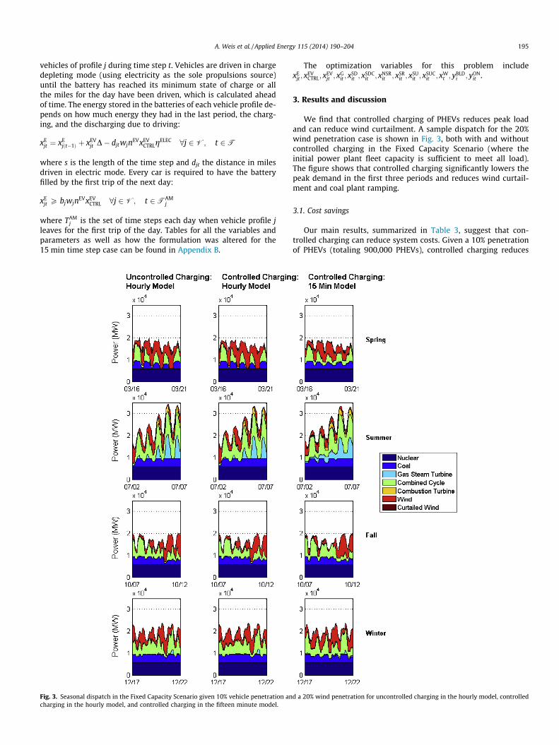
Fig. 3. Seasonal dispatch in the Fixed Capacity Scenario given 10% vehicle penetration ancharging in the hourly model, and controlled charging in the fifteen minute model.
The optimization variables for this problem includexE
jt; xEVCTRL; x
EVjt ; x
Git ; x
SDit ; x
SDCit ; xNSR
it ; xSRit ; x
SUit ; x
SUCit ; xW
t ; yBLDi ; yON
it .
3. Results and discussion
We find that controlled charging of PHEVs reduces peak loadand can reduce wind curtailment. A sample dispatch for the 20%wind penetration case is shown in Fig. 3, both with and withoutcontrolled charging in the Fixed Capacity Scenario (where theinitial power plant fleet capacity is sufficient to meet all load).The figure shows that controlled charging significantly lowers thepeak demand in the first three periods and reduces wind curtail-ment and coal plant ramping.
3.1. Cost savings
Our main results, summarized in Table 3, suggest that con-trolled charging can reduce system costs. Given a 10% penetrationof PHEVs (totaling 900,000 PHEVs), controlled charging reduces
d a 20% wind penetration for uncontrolled charging in the hourly model, controlled

Table 3Comparison of cost savings from controlled PHEV charging in the Fixed Capacity Scenario and Capacity Expansion Scenario for a 0% and 20% wind penetration, given differentcharging scenarios: Uncontrolled Charging, which uses the entire set of vehicles from the NHTS and begins as soon as the vehicle arrives home for the day; Delayed Charging,which also uses the entire set of vehicles from the NHTS and begins charging as late as possible before the vehicle leaves for the next day’s trip while still achieving maximalcharge; and Controlled Charging, which uses the weighted set of 20 representative vehicles and optimally charges each vehicle as part of the dispatch optimization, given a $0payment to vehicle owners for participation. The maximum savings are calculated as the difference between the Uncontrolled and Controlled Charging system costs. The systemcosts for each system without plug-in hybrid electric vehicles are given as a reference, and reduction in vehicle integration costs is found by dividing the difference in costsbetween uncontrolled charging vs. controlled charging with difference in costs between uncontrolled charging vs. no vehicles.
Fixed capacity scenario (starting capacity:34,700 MW)
Capacity expansion scenario (startingcapacity: 27,500 MW)
0% Windpenetration
20% Windpenetration
0% Windpenetration
20% Windpenetration
A. System costs with no PHEVs (reference) 3.56 $billion/year 4.42 $billion/year 4.05 $billion/year 4.89 $billion/yearB. System costs with uncontrolled charging 3.69 $billion/year 4.53 $billion/year 4.20 $billion/year 5.04 $billion/yearC. System costs with delayed charging 3.65 $billion/year 4.49 $billion/year 4.18 $billion/year 4.98 $billion/yearD. System costs with 100% controlled charging and $0 payment to vehicle
owners3.62 $billion/year 4.46 $billion/year 4.10 $billion/year 4.93 $billion/year
Maximum cost savings with controlled charging [B–D] 65 $million/year 69 $million/year 97 $million/year 110 $million/yearOperational cost savings%, capital cost savings% 100%, 0% 100%, 0% �27%, 127% 30%, 70%Reduction in vehicle integration costs with controlled charging
[(B–D)/(B–A)]54% 63% 66% 73%
196 A. Weis et al. / Applied Energy 115 (2014) 190–204
power generation costs by $65–$110 million dollars a year com-pared to the uncontrolled charging scenario, representing 1.5–2.3% of total system costs and 54–73% of the cost of integratingPHEVs. Controlled vehicle charging allows for shifting generationto cheaper plants and to off-peak hours. As shown in Table 3, con-trolled charging is most valuable in the Capacity Expansion Sce-nario, as the controlled charging program offers the opportunityto change which types and how many new power plants are built,in addition to influencing plant operation. In the Fixed CapacityScenario, the additional vehicle load can be accommodated with-out building any new capacity, as the system is already operatingwith more capacity than required by the 15% reserve margin. Inall cases, delayed charging is able to capture some, but not all, ofthe cost reductions offered by controlled charging. It is interestingto note that, regardless of the capacity scenario, when there is a20% wind penetration, controlled charging offers 6–13% greatercost reduction compared to the same system without wind. Thus,most of the cost savings can be captured even when there is nowind in the system, and savings are somewhat higher but not dra-matically higher in a system with significant wind generation. Adetailed breakdown of the costs for each payment level in each sce-nario can found in Appendix C.
There are limitations to these results. On one hand, they mayoverestimate the value of controlled charging by assuming perfectknowledge of vehicle trips and wind generation. Ensuring fullcharge of vehicles each day when vehicle trips and wind genera-tion are uncertain may require safety margins that limit the flexi-bility of controlled charging, and implementable controllers withlimited information about future states will have lower savingsthan optimal solutions under perfect information. On the otherhand, controlled charging may provide additional value to the gridwhen accounting for the forecasting error of wind generation, asvehicle charging can be changed on time scales much faster thanthe ramping constraints of conventional power plants. Addition-ally, while we allow charging only at home, availability of work-place or public charging might increase the flexibility and valueof controlled charging (though the availability of low cost plantswill continue to encourage most charging at night at home). Exceptfor the wind power, we assume that power plants are not limitedby availability because with a limited number of sample days itis difficult to predict which plants might be offline. This assump-tion could overestimate the flexibility in the system and thereforeunder-estimate the benefits of controlled charging. However, withthe exception of nuclear plants, none of the plant types run 100% ofthe time, so we do not expect cost estimates to be substantially
affected by plant downtime. This assumption also does not changethe value in the Capacity Expansion Scenario, as reserve marginsdo not take availability into account but only reference peak loadand total capacity. We also do not consider the costs maintainingwind farms or replacing them if they fail. While these costs couldsignificantly increase the total costs of wind farms, it should signif-icantly impact the interaction of vehicle charging and wind. Elec-tric vehicles would not change any of these costs and if less windis on the system it could only decrease the modest difference be-tween the value of controlled charging with high vs. low wind pen-etrations. Additionally, we ignore transmission constraints, whichmay over- or under-estimate this value depending on the distribu-tion of PHEVs and other flexible resources in congested areas of thegrid. It is possible that controlled charging of PHEVs could provideadditional value by mitigating transmission congestion, but theymay be unable to absorb wind energy if separated from wind re-sources by congested areas of the grid. The results from this modeldo give a good estimate of the operational cost savings possibleconsidering time scales greater than an hour. And because the costreductions result largely from shifting peak load, they should re-main relatively unchanged with more detailed models.
We examined the sensitivity of the cost savings to several dif-ferent important input assumptions, the first of which is the hourlytime scale. We optimized grid operations over the same twenty-day period with a fifteen minute time scale using a modified ver-sion of the optimization model designed to handle larger problems,without capacity expansion, by optimizing each day’s dispatchsequentially, as described further in Appendix B. This allowed formanageable runtimes even with four times as many variables perday, while obtaining solutions close to the optimal solution ofthe original model. Total system costs for a 10% vehicle penetrationwith uncontrolled charging were �2% higher in the fifteen minutemodel given a 0% wind penetration, and �7% higher given a 20%wind penetration compared to the hourly model. Higher systemcosts are expected especially in the high wind case because thereis more total ramping to accommodate the shorter time scaleexamined. The cost reductions associated with controlled chargingare slightly lower in the fifteen-minute model, as shown in Fig. 4.The higher time resolution of the data leads to a lower peak de-mand in the uncontrolled charging case. This effect overwhelmsany additional cost reductions that might occur at fifteen-minutetime resolution due to additional flexibility, and indicates thatthe cost reduction estimates at hourly resolution are optimistic.Both time resolutions produce similar trends between 0% and20% wind penetration given the same initial generation capacity.

Fig. 4. Annual cost savings due to controlled charging for different models given 0%and 20% wind penetration.
A. Weis et al. / Applied Energy 115 (2014) 190–204 197
These results suggest that the hourly time scale used in the basecase is likely sufficient resolution – it does not miss a major sourceof benefits from controlled charging at higher resolution. Althoughit is possible that even shorter time scales may allow for controlledcharging to provide more benefit through participation in the reg-ulation market, this requires more extensive communication infra-structure, and this market is expected to saturate with a relativelysmall number of vehicles [9]. In addition, the fifteen minute loadcontrol framework is similar to many existing demand responseprograms that use one-way radio controlled switches and cycleloads roughly every 15 min [28].
We also investigated the sensitivity of the results to changes inthe parameters of the PHEV fleet. The potential cost savings fromcontrolled charging is approximately linear with the penetrationof PHEVs, as shown in Fig. 5. Regardless of the vehicle penetration,controlled charging is worth more in scenarios with high windpenetration and capacity expansion. In the Capacity Expansion Sce-nario with 20% wind penetration, the cost reduction is slightlyhigher than the linear trend at the 15% vehicle penetration becausecontrolled charging prevents construction of an additional gasplant. The Fixed Capacity Scenario with 20% wind penetrationhas a slightly higher cost reduction at 10% vehicle penetration thanthe linear trend because it has the most switching away from gasturbine generation.
Fig. 5. Sensitivity of the maximum annual system cost savings possible through100% controlled electric vehicle charging compared to uncontrolled charging for arange of vehicle penetrations from 0% to 15% of a 9 million passenger vehicle fleet.
Increasing the maximum charge rates has diminishing returns,as shown in Fig. 6. Level 1 charging restricts the peak power thatoccurs with uncontrolled charging, so controlling the charging ismuch less valuable. In the uncontrolled charging scenarios,increasing to Level 3 charging from Level 2 charging only mini-mally increases the peak load because the total amount all vehiclescan be charged is limited by battery size and total driving distance.As battery size increases, the vehicles are able to drive more milesper day in charge depleting mode. This increases the value of con-trolled charging to the system somewhat, as the uncontrolled peakload becomes more and more expensive. However, this benefit islimited because the more miles traveled in charge depleting mode,the less flexibility there is to move charging to a later time, sincemuch of the time spent parked is needed for charging. Examininga range of 5 kW h batteries to 24 kW h batteries, we see cost reduc-tions differ from the base case by $1–$35 million dollars per yeardepending on the scenario due to the competing effects discussedabove.
3.2. Capacity and generation mix
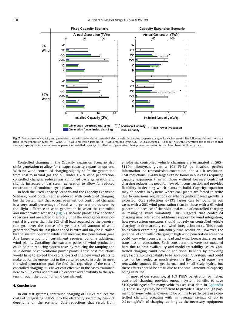
Fig. 7 summarizes plant capacity and generation results for fourcases. In the Fixed Capacity Scenario with no wind, controlledcharging reduces generation from gas-combined cycle and oil/gassteam plants and increases generation from coal plants slightly,bringing coal plants to very high utilization levels. The lack of boththe cheap energy from wind and its variability means that any coalcapacity is utilized nearly continuously with very few startups andshutdowns. Not surprisingly, in the Fixed Capacity Scenario undera 20% wind penetration, controlled charging results in reducedgeneration from all fossil fuel plants types, replacing it with windgeneration.
In the Capacity Expansion Scenario, controlled charging resultsin reduced plant construction: when there is no wind, fewer gascombined cycle and coal plants are built; and for a 20% wind pen-etration, no additional coal plants are built because of the abun-dance of low cost and high variability wind. Instead, mostadditional capacity is combined cycle gas. Given controlled charg-ing, far fewer combustion plants are built compared to the uncon-trolled charging scenario, and in exchange a small number of gasturbine plants are built to meet reserve margin and rampingrequirements. These plants have higher operating costs than coaland combined cycle plants but have the lowest capital costs.
Fig. 6. Sensitivity of the maximum annual system cost savings possible through100% controlled electric vehicle charging compared to uncontrolled charging forLevel 1 (1.2 kW), Level 2 (7.4 kW), and Level 3 (30 kW) charging. Only Level 1 and 2are likely to be used in residential settings in the foreseeable future.
Fixed Capacity Scenario Capacity Expansion Scenario
0% Wind
20% Wind
Fig. 7. Comparison of capacity and generation data with and without controlled electric vehicle charging by generator type for each scenario. The following abbreviations areused for the generation types: W – Wind, CT – Gas Combustion Turbine, CC – Gas Combined Cycle, O/G – Oil/Gas Steam, C – Coal, N – Nuclear. Generation axis is scaled so thataverage capacity factor can be seen as percent of installed capacity bar filled with generation. Peak power production is calculated based on hourly data.
198 A. Weis et al. / Applied Energy 115 (2014) 190–204
Controlled charging in the Capacity Expansion Scenario alsoshifts generation to allow for cheaper capacity expansion options.With no wind, controlled charging slightly shifts the generationfrom coal to natural gas and oil. Under a 20% wind penetration,controlled charging reduces gas combined cycle generation andslightly increases oil/gas steam generation to allow for reducedconstruction of combined cycle plants.
In both the Fixed Capacity Scenario and the Capacity ExpansionScenario, wind curtailment is reduced with controlled charging,but the curtailment that occurs even without controlled chargingis a very small percentage of total wind generation, as seen bythe slight difference in wind generation between the controlledand uncontrolled scenarios (Fig. 7). Because plants have specifiedcapacities and are added discretely until the wind generation po-tential is greater than the 20% of all load required by the penetra-tion goal over the course of a year, a small amount of windgeneration from the last plant added is extra and may be curtailedby the system operator while still meeting the penetration goal.Any larger amount of curtailment requires building additionalwind plants. Curtailing the extreme peaks of wind productioncould help in reducing system costs by reducing the ramping andshut downs of conventional power plants. These cost reductionswould have to exceed the capital costs of the new wind plants tomake up for the energy lost in the curtailed peaks in order to meetthe wind penetration goal. We find that regardless of the cost ofcontrolled charging, it is never cost effective in the cases examinedhere to build extra wind plants in order to add flexibility to the sys-tem through the option of wind curtailment.
4. Conclusions
In our test systems, controlled charging of PHEVs reduces thecosts of integrating PHEVs into the electricity system by 54–73%depending on the scenario. Cost reductions that result from
employing controlled vehicle charging are estimated at $65–$110 million/year, given a 10% PHEV penetration, perfectinformation, no transmission constraints, and a 1-h resolution.Cost reductions 50–60% larger can be found in our cases requiringcapacity expansion than in those without because controlledcharging reduces the need for new plant construction and providesflexibility in deciding which plants to build. Capacity expansionmay be needed in systems where coal plants are forced to retiredue to emissions regulations or when significant load growth isexpected. Cost reductions 6–13% larger can be found in ourcases with a 20% wind penetration than in those with a 0% windpenetration because of the additional value of controlled chargingin managing wind variability. This suggests that controlledcharging may offer some additional support for wind integration;however, system operators should not rely on controlled vehiclecharging to dramatically cut wind integration costs. This resultholds when examining sub-hourly time resolution. However, thepotential of controlled charging in high wind penetration scenarioscould vary when considering load and wind forecasting error andtransmission constraints. Such considerations were not modeledhere due to data availability and model tractability issues. Con-trolled charging could provide additional benefits by providingvery fast ramping capability to balance solar PV systems, and couldalso not be needed as much given the flexibility of some newrenewable sources like geothermal and small scale hydro, butthese effects should be small due to the small amount of capacitybeing installed.
In most of our scenarios, at 10% PHEV penetration or higher,controlled charging provides enough system benefits to save$100/vehicle/year for many vehicles (see cost data in AppendixC). These savings may be sufficient to provide a large enough pay-ment for some vehicles owners to be willing to participate in a con-trolled charging program with an average savings of up to0.2 cents/kW h of charging, as long as the necessary equipment

A. Weis et al. / Applied Energy 115 (2014) 190–204 199
can be obtained by the vehicle owner or system operator at lowcost. Both the installation and maintenance costs of the controlledcharging system would have to come out of the $100/vehicle/year.The cost benefits of controlled charging scale fairly linearly withthe number of PHEVs, so if the equipment costs per vehicle arelow enough and the overhead costs of program are kept low, a con-trolled charging program could pay for itself even at low PHEVpenetrations. We do not, however, model the vehicle owner’s will-ingness to participate in the program, as this is a behavioral ques-tion beyond the scope of our analysis.
Building additional wind plants beyond the penetration goal inorder to allow curtailment and mitigate extreme generation fluctu-ation is not cost effective in our model. Although the energy lost bycurtailing peaks is minimal and therefore requires little additionalcapacity to make up for it, the high capital cost of wind farms out-weighs any benefit of flexibility to the grid.
Acknowledgements
The authors would like to thank Bri-Mathias Hodge for his feed-back and guidance on our modeling efforts and to David Luke Oatesfor technical assistance. This work was supported through theRenewElec Project (http://www.renewelec.org) by the Doris DukeCharitable Foundation, the Richard King Mellon Foundation, theElectric Power Research Institute, and the Heinz Endowment. Addi-tional funding was provided by the National Science FoundationCAREER Award #0747911 and the National Science FoundationGraduate Research Fellowship Program. Findings and recommen-
Fig. A.1. Aggregate characteristics for all passenger vehicles in the NHTS dataset and be1 million random draws. The percent of vehicles at home dips during the day, and only
dations are the sole responsibility of the authors and do not neces-sarily represent the views of the sponsors.
Appendix A. Selecting representative driving profiles
The capacity expansion, unit commitment, and dispatch modeluses driving profiles to determine the state of charge of the plug-invehicles in the model. Representative driving profiles are chosenfrom the 2009 National Household Travel Survey (NHTS) data set,which contains data for one day of driving from approximately900,000 different passenger cars across the United States. Theseprofiles include information for each vehicle on all trips taken dur-ing that day, including distance traveled, starting and stoppingtimes, and starting and stopping locations, so that plug-in hybridvehicle expected battery state of charge can be tracked throughoutthe day with a variety of different location-dependent chargingschemes. Vehicles in the controlled charging program are allowedto charge when parked at home after the last trip of the day andmust be fully charged by the first trip of the day. Uncontrolledvehicles begin charging after arriving home for the last time thatday and charge at the maximum rate until fully charged or leavingfor the first trip of the next day. Each vehicle discharges its batterythroughout the day based on the number of miles driven until thebattery reaches its minimum state of charge.
In order to create a tractable controlled charging model whilemaintaining a representative dynamic vehicle load for the powersystem, a sample of 20 profiles were selected and optimallyweighted to best match the aggregate characteristics of the entire900,000 profiles available in the NHTS of passenger cars. These
st match 20 optimally weighted vehicle profiles drawn from the NHTS dataset overa small percentage of the fleet is driving at any time.

Table B.1Optimization variables.
Symbol Description Domain Units
xEjt
Sum of usable energy remaining in all vehicles in controlled charging program of type j in time step t Rþ MW h
xEVCTRL
Percentage of plug-in vehicles in the controlled charging program [0,100] %
xEVjt
Sum of power to charge all vehicles in controlled charging program of type j in time step t Rþ MW
xGit
Power generated in time step t by plant i Rþ MW
xSDit
Shut-down variable for the minimum on/off constraints for plant i at time t. Formulation forces this to 1 (plant shutting down) or 0 (plantnot shutting down)
[0,1] NA
xSDCit
Shut-downs for plant i in time step t Rþ NA
xNSRit
Non-spinning reserve power for plant i in time step t Rþ MW
xSRit
Spinning reserve power for plant i in time step t Rþ MW
xSUit
Start-up variable for the minimum on/off constraints for plant i at time t. Formulation forces this to 1 (plant starting up) or 0 (plant notstarting up)
[0,1] NA
xSUCit
Start-up cost for plant i in time step t Rþ NA
xWt Total wind generation taken in time step t Rþ MW
yBLDi
Binary decision = 1 if plant i is built, 0 otherwise {0,1} NA
yONit
Binary decision = 1 if plant i is on at time i, 0 otherwise {0,1} NA
Table B.2Model parameters.
Symbol Description Base value Sensitivity values Units
bj Battery capacity of vehicle j 16 5, 24 kW hbAM Battery charge requirement in the morning 100/Max possiblea – %
bHIj
Battery higher limit for vehicle j 100 – %
bLOj
Battery lower limit for vehicle j 30 – %
cBLDi
Capital cost of each new plant i EIA 2011 reference case – $/year
cEV Payment to vehicle owner for participation in controlled charging program $0 $100, $200, $300 $/vehicle/yearcF
iFuel cost of plant i EIA 2011 reference case – $/Btu
djt Distance driven by each vehicle of type j in time t NHTS sample – milesERPS RPS energy requirement 10% 0%, 20% %hi Heat rate for plant i Ventyx – Btu/MW hki Size of each plant i Ventyx – MWLt Non-vehicle load at time t NYISO – MWlj Charge limit of vehicle j 9.6 1.2, 30 kWmi Minimum generation for plant i Ventyx – %nEV Number of plug-in vehicles total 10% 1%, 15% % Of total vehiclespwt Wind power potential at time t from each wind plant EWITS data – MWpjt Percent of time step vehicle type j is home NHTS sample – %RSR Spinning reserve requirement 3% – %RTR Total reserve requirement 6% – %RRM Reserve margin over peak load 15% – %rDWN
iRamp down rate for plant i Ventyx – MW/h
rUPi
Ramp up rate for plant i Ventyx – MW/h
vUCTRLt Charging power to all uncontrolled plug-in hybrid electric vehicles at time t NHTS database – MW
wj Weighting factor for vehicles that are of type j NHTS sample – %D Length of time step 1 0.25 h
dOFFi
Minimum time off for plant i WECC – # Time steps
dONi
Minimum time on for plant i WECC – # Time steps
gELEC Efficiency of vehicle in electric mode .3 – kW h/mile
a Vehicles which cannot be charged completely during their longest period at home are always charged for that entire time period.
200 A. Weis et al. / Applied Energy 115 (2014) 190–204
aggregate characteristics were evaluated for each hour and in-cluded the average number of miles driven in that hour, the aver-age cumulative number of miles driven until that hour, the percentof vehicles at home, and the percent of vehicles parked.
20 Vehicle profiles were randomly selected from the NHTS dataset; the characteristics of the resulting fleet were compared tothose of the full NHTS data set using the distance metric below;and this process was repeated one million times, retaining onlythe set of 20 that minimizes the distance metric.
distance metric ¼X
t
Dh2t þ Dp2
t þ Do2t þ Dd2
t þDat
maxtðatÞ
0@
1A2
þ Dct
maxtðctÞ
0@
1A2
0B@
1CA
where Dht and Dpt are the difference in the percent of drivers in thesample vs. the full data set at home and parked at time step t,respectively, and Dat and Dct are the difference in average milesand cumulative miles, respectively, at time step t. The distanceterms are normalized so that all six terms will be of comparablescale. Each of the 20 vehicles was weighted by a variable wi,i 2 {1,2, . . . ,20}, wi 2 [0,1],
Piwi ¼ 1; wi was optimized to minimize
the distance metric above. This process was repeated 1 milliontimes and the best match optimally weighted profile of 20 vehicleswas retained. The weighted sample can be thought of as a casewhere some selected vehicle profiles are representative of a largerportion of the full NHTS dataset than others.As shown in Fig. A.1,the final sample of 20 weighted profiles does not perfectly match

Table C.1Costs given a 0% wind penetration and 10% vehicle penetration with different levels of payment to PHEV owners for controlled charging in the Fixed Capacity Scenario. Overnightnew capital costs include the cost of building wind capacity in order to meet the wind penetration goal as well as any additional plants. Annualized new capital costs represent thecost each year given the lifetime of each plant (50 years for coal, 30 years for gas, and 20 years for wind) and a 5% discount rate.a Annualized new system costs are the sum of theannualized new capital costs, annual vehicle program costs, and annual operating costs.
Vehicle payment ($/vehicle/year)
Percentcontrolled(%)
Overnight new capitalcost (billion $)
Annualized new capitalcosts (billion $)
Annual vehicle programcosts (million $)
Annual operatingcosts (billion $)
Annualized new systemcosts (billion $)
0 100 4.5 0.29 0 3.3 3.6100 48 4.5 0.29 43 3.4 3.7200 0 4.5 0.29 0 3.4 3.7
a The discount rate is highly uncertain because it depends on what else could have been invested in instead of the power plants. The IEA uses provides annualized costs ofpower plants using both a 5% and 10% discount rate [29] while the Office of Management and Budget suggests using a 7% discount rate [30] and experts consulted suggestedrates between 3% and 10%. A higher discount rate would mean that investments in new power plants would be more expensive and therefore increase the value of controlledcharging. Future work can examine a range of discount factors to understand the sensitivity to this parameter.
Table C.2Costs given a 20% wind penetration and 10% vehicle penetration with different levels of payment to PHEV owners for controlled charging in the Fixed Capacity Scenario.
Vehicle payment ($/vehicle/year)
Percentcontrolled(%)
Overnight new capitalcost (billion $)
Annualized new capitalcosts (billion $)
Annual vehicle programcosts (million $)
Annual operatingcosts (billion $)
Annualized new systemcosts (billion $)
0 100 25 2.0 0 2.5 4.5100 0 25 2.0 0 2.5 4.5
Table C.3Costs given a 0% wind penetration and 10% vehicle penetration with different levels of payment to PHEV owners for controlled charging in the Capacity Expansion Scenario.
Vehicle payment ($/vehicle/year)
Percentcontrolled(%)
Overnight new capitalcost (billion $)
Annualized new capitalcosts (billion $)
Annual vehicle programcosts (million $)
Annual operatingcosts (billion $)
Annualized new systemcosts (billion $)
0 100 10 0.65 0 3.5 4.1100 37 11 0.74 0.03 3.4 4.2200 7.2 12 0.77 0.01 3.4 4.2300 0 12 0.8 0 3.4 4.2
Table C.4Costs given a 20% wind penetration and 10% vehicle penetration with different levels of payment to PHEV owners for controlled charging in the Capacity Expansion Scenario.
Vehicle payment ($/vehicle/year)
Percentcontrolled(%)
Overnight capitalcost (billion $)
Annualized new capitalcosts (billion $)
Annual vehicle programcosts (million $)
Annual operatingcosts (billion $)
Annualized new systemcosts (billion $)
0 100 30 2.3 0 2.6 4.9100 94 30 2.3 0.085 2.6 5.0200 0 31 2.4 0 2.6 5.0
A. Weis et al. / Applied Energy 115 (2014) 190–204 201
the aggregate characteristics of all passenger vehicles. However, itmuch more closely matches the aggregate data than 20 randomlychosen profiles and according to the distance metric shown below,it is just as close as 200 randomly chosen profiles and allows for afeasible computation time. While we track day-to-day differencesin wind and load, we assume that vehicle travel patterns are thesame every day (due to lack of data on daily variability).
Appendix B. Optimization variables and parameters
See Tables B.1 and B.2.
B.1. Fifteen minute model
For the fifteen minute model, most of the constraints remainthe same, but everything regarding capacity expansion is removedfrom the objective function and constraints. Additionally, insteadof executing the full twenty day period at once, we optimize over
a 48 h window, save the first 24 h of data as the optimal operationfor that day, move the window forward 24 h and run another 48 hoptimization. This is repeated until optimal operation has beenfound for all 20 days. This shorter optimization window allowsfor a greater time resolution in the data while retaining similarrun times. The new objective function used for each 48 h periodis shown below. By removing the payment to vehicle owners fromthe objective function, we assume a $0/vehicle/year payment in allcases and separately dictate xEV
CTRL as 1 or 0. For the sensitivity anal-ysis, we are only interested in the extremes of all vehicles beingcontrolled or none to understand the largest possible cost savings.
Minimize the cost operating costs in each time step:
minimizeX
t2T48
Xi2C
xSUCit þ xSDC
it þ cFi hixG
it
� �� �|fflfflfflfflfflfflfflfflfflfflfflfflfflfflfflfflfflfflfflfflfflfflfflfflfflfflfflfflfflfflfflfflfflfflfflffl{zfflfflfflfflfflfflfflfflfflfflfflfflfflfflfflfflfflfflfflfflfflfflfflfflfflfflfflfflfflfflfflfflfflfflfflffl}
Cost of Plant Operations
No additional plants are provided to be built, so the constraintrequiring plants to be built in order to be turned on is dropped.

Fig. C.1. Comparison of resulting generation mixes between the hourly and fifteenminute model.
Table C.5Capacity factor for each generation type given a 0% wind penetration and 10% vehicle penFixed Capacity Scenario.
Vehicle payment ($/vehicle/year) Percent controlled (%) Nuclear (%) Coal (%
0 100 100 98100 48 100 97200 0 100 97
Table C.6Capacity factor for each generation type given a 20% wind penetration and 10% vehicle peneFixed Capacity Scenario.
Vehicle payment ($/vehicle/year)
Percent controlled(%)
Nuclear(%)
Coal(%)
Oil(%)
0 100 100 81 4.4100 0 100 82 4.9
Table C.7Capacity factor for each generation type given a 0% wind penetration and 10% vehicle peneCapacity Expansion Scenario.
Vehicle payment ($/vehicle/year) Percent controlled (%) Nuclear (%) Coal (%
0 100 100 97100 37 100 96200 7.2 100 96300 0 100 96
Table C.8Capacity factor for each generation type given a 20% wind penetration and 10% vehicle peneCapacity Expansion Scenario.
Vehicle payment ($/vehicle/year)
Percent controlled(%)
Nuclear(%)
Coal(%)
Oil(%)
0 100 100 86 5.3100 94 100 85 5.1200 0 100 85 4.4
202 A. Weis et al. / Applied Energy 115 (2014) 190–204
The wind penetration target requirement is also dropped because itcan only be used across all time periods at once. Instead, we assumethat the wind penetration functions simply as a requirement tobuild sufficient wind capacity so that 20% of the energy could begenerated by wind. The model uses the same set of wind farms asused in the hourly model with 20% wind penetration. Because ofthe low marginal cost of wind, most of this wind energy will be usedwithout a hard constraint. Constraints are added to hold the unitcommitment variables constant through a single hour so that plantscan only be turned off or turned on each hour, while generation lev-els are free to change every fifteen minutes.
Appendix C. Additional results
C.1. Detailed cost breakdown
In Tables C.1–C.4, the operational and capital costs are brokendown for each scenario. In each case, the higher the payment thatthe grid operator is assumed to pay to each individual vehicle own-er, the lower the number of vehicles it is optimal for the grid oper-ator to include in the charging program.
C.2. Generation mix
The generation mix remains fairly similar between the hourlyand fifteen minute model. The most noticeable differences arethe increased use of oil/gas steam turbines and combustion
etration with different levels of payment PHEV owners for controlled charging in the
) Oil/gas steam (%) Gas combined cycle (%) Gas combustion turbine (%)
7 73 127 73 128 74 12
tration with different levels of payment to PHEV owners for controlled charging in the
/gas steam Gas combined cycle(%)
Gas combustion turbine(%)
Wind(%)
47 6.5 3648 6.6 36
tration with different levels of payment to PHEV owners for controlled charging in the
) Oil/gas steam (%) Gas combined cycle (%) Gas combustion turbine (%)
7.0 54 2.87.0 50 2.36.2 49 2.46.1 49 2.4
tration with different levels of payment to PHEV owners for controlled charging in the
/gas steam Gas combined cycle(%)
Gas combustion turbine(%)
Wind(%)
38 2.2 3639 2.0 3636 1.2 36

Table DModel Assumptions. (�) Represents assumptions that we believe result in our model underestimating the benefits of controlled charging. (+) Represents assumptions that canresult in our model overestimating the benefits.
Assumption Justification Expected direction of bias of the value of controlled charging
No transmission constraints No data available (�) In our model, uncontrolled charging does not increasecongestion and controlled is given no chance to relieve thisand other congestion in the system
Perfect information for demand andwind
Limited forecasting data available for the future wind sites,and this would require assumptions about the structure offuture reserve markets to value the service
(�) Controlled charging may be able to help forecasting error
Hourly time steps Increasing the time step to 15 min does not qualitativelychange the results, and use of hourly time steps allows manymore scenarios to be examined. The variability of winddecreases with frequency [14] so substantial differences atsmaller time steps are unlikely
(�) Some of the fast balancing that can be performed bycontrolled charging is missed, but we expect it to be small
Battery can be charged anywherebetween 0 and its maximumcharge rate
While instantaneous changes in charge rate may be limited, atan hourly time scale, the desired average charge rate can beachieved without technical challenges
We do not expect this assumption to be unrealistic at the timescales examined
We focus on extended range plug-inhybrid electric vehicles instead ofvehicles with blended operation
Although not the case for every PHEV, the Chevy Volt depletesthe battery before extending the range with the gasolinemotor as opposed to operating in a blended mode. Likeprevious studies [12,14], we assume our PHEV’s operate as anextended range vehicle like the Chevy Volt
(+) Blended operation PHEVs result in somewhat smallerelectricity demand for the same battery size, reducing theimpact of uncontrolled charging and the potential forcontrolled charging to reduce this impact. We expect this tobe a small effect, as a blended mode is more common invehicles with smaller batteries where daily driving patternsare likely to use the entire battery even in blended mode.Modeling blended-operation PHEVs requires assumptionsabout vehicle control strategies, but there is no reason tobelieve these small differences in electricity consumptionwould qualitatively change results
Controlled charging does notsignificantly reduce battery life
Degradation is complex, so we cannot be certain, but weexpect that controlled charging will not decrease battery lifeand may increase it. Barre et al. review the literature onlithium-ion battery aging mechanisms and find that cyclenumber is the most important factor, but voltage,temperature, and change in SOC can also play a factor [10].Controlled charging does not change the number of cycles,and because it lowers the average C-rate, may decreaseaverage charging voltage and temperature and thereforepotentially extend battery life. Controlled charging alsochanges how long batteries remain at low SOC vs. high SOCwhile plugged in. Some chemistries have been shown todegrade faster at high SOC, so again controlled charging mayextend battery life by leaving batteries at low SOC longerbefore charging rather than charging immediately uponarrival
(�) The benefits of controlled charging may be larger if thereduced average C-rate of controlled charging results inextended battery life. However, it is not known whethervariation in C-rate or SOC profile may have other positive ornegative effects on battery life
20 days are used to represent thecalendar year
Necessary due to computational constraints in order toexamine a wide variety of sensitivity cases
This could shift the results in either direction, but we expectthe differences to be small since the average load and windmatch the annual averages and the peak and minimum loadconditions are captured
A. Weis et al. / Applied Energy 115 (2014) 190–204 203
turbines with the fifteen minute model, and a corresponding de-crease in the use of combined cycle plants. Wind energy is alsoused less with the fifteen minute model because we dropped thehard wind energy constraint in order to perform each day’s optimi-zation separately to save computation time with larger number oftime steps. Using the same wind capacity as in the Fixed CapacityScenario hourly model, the fifteen minute model had only 19%wind by energy.
C.3. Capacity factors
In the Fixed Capacity Scenario, combined cycle plants have alower capacity factor when charging is controlled. All conventionalpower plants except for nuclear which is held at 100% of its capac-ity at all times have a lower capacity factor under 20% wind pene-tration compared to a 0% wind penetration (see Fig. C.1 and TablesC.5–C.8).
In low initial capacity scenarios combined cycle plants have ahigher capacity factor with controlled charging as the controlledcharging allowed for fewer combined cycle plants to be built.
Appendix D. Assumptions
Table D discusses the assumptions made in the study and theexpected direction and magnitude of bias they might give theresults.
References
[1] US Energy Information Administration. Emissions of Greenhouse Gases in theUnited States 2008; 2008. <http://www.eia.gov/oiaf/1605/ggrpt/pdf/0573%282008%29.pdf> [accessed 24.03.13].
[2] DSIRE RPS Data Spreadsheet. 2012. <http://www.dsireusa.org/rpsdata/index.cfm> [accessed 24.03.13].
[3] Katzenstein W, Apt J. Air emissions due to wind and solar power. Environ SciTechnol 2009;43(2):253–8.
[4] Office of Energy Projects FERC, December 2012 Energy Infrastructure Report.December 2012. <http://www.ferc.gov/legal/staff-reports/dec-2012-energy-infrastructure.pdf> [accessed 18.06.13].
[5] Michalek JJ, Chester M, Jaramillo P, Samaras C, Shiau C-SN, Lave LB. Valuationof plug-in vehicle life-cycle air emissions and oil displacement benefits. PNAS2011;108(40):16554–8.
[6] Peterson SB, Whitacre JF, Apt J. Net air emissions from electric vehicles: theeffect of carbon price and charging strategies. Environ Sci Technol2011;45(5):1792–7.

204 A. Weis et al. / Applied Energy 115 (2014) 190–204
[7] Lund H, Kempton W. Integration of renewable energy into the transport andelectricity sectors through V2G. Energy Policy 2008;36(9):3578–87.
[8] Kristoffersen T, Capion K, Meiborn P. Optimal charging of electric drivevehicles in a market environment. Appl Energy 2011;88:1940–8.
[9] Peterson SB, Whitacre JF, Apt J. The economics of using plug-in hybrid electricvehicle battery packs for grid storage. J Power Sources 2010;195:2377–84.
[10] Barre A, Deguilhem B, Grolleau S, Gerard M, Suard F, Riu D. A review onlithium-ion battery ageing mechanisms and estimations for automotiveapplications. J Power Sources 2013;241:680–9.
[11] Dallinger D, Gerda S, Wietschel Martin. ‘‘Integration of intermittent renewablepower supply using grid-connected vehicles – a 2030 case study for Californiaand Germany’’. Appl Energy 2013;104:666–82.
[12] Foley A, Tyther B, Calnan P, Gallachoir B. Impacts of Electric Vehicle chargingunder electricity market operations. Appl Energy 2013;101:93–102.
[13] Wang J, Liu C, Ton D, Zhou Y, Kim J, Vyas A. Impact of plug-in hybrid electricvehicles on power systems with demand response and wind power. EnergyPolicy 2011;39(7):4016–21.
[14] Katzenstein W, Fertig E, Apt J. The variability of interconnected wind plants.Energy Policy 2010;38(8):4400–10.
[15] Sioshansi R, Denholm P. The value of plug-in hybrid electric vehicles as gridresources. Energy J 2010;31(3):1–10.
[16] De Jonghe C, Delarue E, Belmans R, D’haeseleer W. Determining optimalelectricity technology mix with high level of wind power penetration. ApplEnergy 2011;88:2231–8.
[17] Tuffner F, Kintner-Meyer M. PNNL ‘‘using electric vehicles to meet balancingrequirements associated with wind power’’; 2011.
[18] Druitt J, Früh W-G. Simulation of demand management and grid balancingwith electric vehicles. J Power Sources 2012;216:104–16.
[19] Ventyx. Velocity suite; 2011.[20] EPA. National Electric Energy Data System (NEEDS); 2010.[21] US Department of Transportation. Federal highway administration. 2009
National Household Travel Survey; 2009. <http://nhts.ornl.gov> [accessed10.06.11].
[22] State of New York Public Service Commission. ‘‘CASE 13-E-0199 – In theMatter of Electric Vehicle Policies’’; May 22, 2013.
[23] Federal Highway Administration. State Statistical Abstract 2008 New York.<http://www.fhwa.dot.gov/policyinformation/statistics/abstracts/ny.cfm>[accessed 04.07.13].
[24] EIA. Annual energy outlook 2011 with projections to 2035; 2010.[25] NREL. Eastern wind dataset. <http://www.nrel.gov/electricity/transmission/
eastern_wind_dataset.html> [accessed 07.07.11].[26] EIA. Annual energy outlook 2010 with projections to 2035; 2010.[27] NERC. Planning reserve margin. <http://www.nerc.com/pa/RAPA/ri/Pages/
PlanningReserveMargin.aspx> [accedssed 12.07.13].[28] Newsham GR, Bowker BG. The effect of utility time-varying pricing and load
control strategies on residential summer peak electricity use: a review. EnergyPolicy 2010;38(7):3289–96.
[29] International Energy Association. Projected cost of generating electricity;2010.
[30] Office of Budget and Management. Circular No. A-94 Revised. Guildines anddiscount rates for benefit-cost analyis of federal programs; October 29, 1992.<http://www.Whitehouse.Gov/omb/Circulars_A094> [accesssed 04.07.13].