ESTIMATING THE TAILS OF LOSS SEVERITY DISTRIBUTIOINS USING EXTREME VALUE THEORY

ALEXANDER J. MCNEIL

Departement Mathematlk ETH Zentrum

CH-8092 Zurich

March 7, 1997

A B S T R A C T

Good estimates for the tails of loss severity dustrlbutlons are essential for pricing or positioning high-excess loss layers m reinsurance We describe parametric curve- fitting inethods for modelling extreme h~storlcal losses These methods revolve around the genelahzed Pareto distribution and are supported by extreme value theory. We summarize relevant theoretical results and provide an extenswe example of thmr ap- plication to Danish data on large fire insurance losses

K E Y W O R D S

Loss severity distributions, high excess layers; exuelne value theory, excesses over high thresholds; generalized Pareto distribution

1 INTROI)UCTION

Insurance products can be priced using our expermnce of losses in the past We can use data on historical loss severities to predict the size of future losses One approach is to fit parametric dtsmbutlons to these data to obtain a model for the underlying loss

severity dlstnbutuon; a standard refelence ozl this practice is Hogg & Klugman (1984).

In thls paper we are specifically interested in modelhng the tails of loss severity distributions Thus is of particular relevance in reinsurance ff we ale required to choose or price a high-excess layer In this SltUatmn it is essential to find a good statistical model for the largest observed historical losses It is less unportant that the model explains slnaller losses, if slnaller losses were also of interest we could Ln any case use a m~xture dlstrlbutmn so that one model apphed to the taft and another to the mare body of the data However, a single model chosen for its ovelall fit to all historical losses may not provide a particularly good fit to the large losses and may not be suita- ble for pricing a high-excess layer

Our modelhng is based on extreme value theory (EVT), a theory whmh until coln- paratlvely recently has found more apphcatlon m hydrology and chlnatology (de Haan

ASTINBULLETIN, Vol 27. No I 1997 pp 117-1"17

118 ALEXANDER J MC NEll.

1990, Smith 1989) than in insurance As Its name suggests, this theory is concerned with the modelhng of extreme events and m the last few years various authors (Be~rlant & Teugels 1992, Embrechts & Kluppelberg 1993) have noted that the theory is as relevant to the modelhng of extreme insurance losses as it ~s to the modelhng of high river levels or temperatures.

For our purposes, the key result in EVT is the Pickands-Balkema-de Haan theorem

(Balkema & de Haan 1974, Pickands 1975) which essentially says that, for a wide class of distributions, losses which exceed high enough thresholds follow the generah- zed Pareto d~strlbutlon (GPD) In this paper we are concerned w~th fitting the GPD to data on exceedances of high thresholds This modelling approach was developed in Davlson (1984), Davlson & Smith (1990) and other papers by these authors

To illustrate the methods, we analyse Danish data on major fire insurance losses.

We provide an extended worked example where we try to point out the pitfalls and hm~tatlons of the methods as well their considerable strengths

2 MODELLING LOSS SEVERITIES

2.1 The context

Suppose insurance losses are denoted by the independent. ~dentlcally distributed ran- dom variables X~. X2, . whose common distribution function is Fx (x) = P{X < ,t} where x > 0 We assume that we are dealing with losses of the same general type and that these loss amounts are adJusted for inflation so as to be comparable.

Now, suppose we are interested m a high-excess loss layer with lower and upper

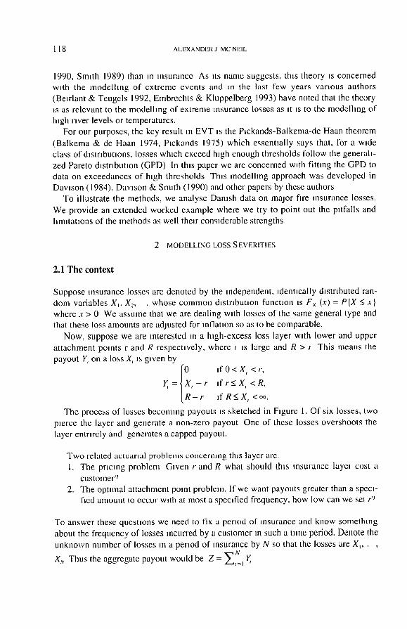
attachment points r and R respectively, where p is large and R > J This means the payout Y, on a loss X, is given by

I 0 i f 0 < X , < r ,

Y, = X, - r if r_< X, < R,

L R - r l fR<_X,<o~.

The process of losses becoming payouts is sketched in Figure 1. Of six losses, two pierce the layer and generate a non-zero payout One of these losses overshoots the

layer entnrely and generates a capped payout.

Two related actuarial problems concerning this layer are. 1. The pricing problem Given r and R what should this insurance layer cost a

customer 9 2. The optimal attachment point problem. If we want payouts greater than a spec~-

fled amount to occur with at most a specified frequency, how low can we set r?

To answer these questions we need to fix a period of insurance and know something about the frequency of losses incurred by a customer in such a tnne period. Denote the

unknown number of losses m a period of insurance by N so that the losses are X~,. ,

Xu Thus the aggregate payout would be Z = y~'~] Y,

ES FIMAq ING THE TAILS OF LOSS SEVERITY DISTRIBU FIONS USING EXTREME VALUE THEORY I 19

X

T X

1 Y1

FIGURE I Possible reahzat~ons of losses m futurc tm~c period

t

A c o m m o n way of pricing is to use the formula Price = E[Z] + k.var[Z], so that the

price is the expected payout plus a risk loading which is k t imes the var iance of the

payout, for some k This is known as the variance pricing principle and it requires only

that we can calculate the first two molnents of Z

The expected payout E[Z] is known as the pure pre lmum and it can be shown to be

E[Y,]E[N]. It is c lear that ,f we wish to price the cove r provided by the layer (r,R)

using the variance principle we must be able to calculate E[Y,], the pure premluln for a

single loss We will calculate E[Y,] as a s imple price Indication in later analyses in this

paper Howeve r , we note that the var iance pricing pr inciple ~s unsophis t ica ted and

may have its drawbacks in heavy tailed si tuations, since moments may not exist or

may be very large An insurance company general ly wishes payouts to be rare events

so that one possible way of fol mula tmg the at tachment point problem might be choo-

se r such that P{Z > 0} < p for some stipulated small probabdlty p That is to say, r is

determined so that in the period ot insurance a non-zero aggregate payout occurs with

probabdlty at most p

The a t tachment point p roblem essent ia l ly bolls down to the estHnatlon o f a high

quant l le of the loss s even ty distr ibution F~(x) In both of these problems we need ~,

good est imate of the loss severi ty dlStrlbul~on for x large, that is to say, In the taft area We must also have a good es t imate o f the loss f requency distr ibution of N, but this

wdl not be a topic ot this paper

2.2 Data Analysis

Typica l ly we will have historical data on losses which exceed a certain amount known

as a d isp lacement It is practically impossible to col lect data on all losses and data on

120 ALEXANDER J MC NElL

small losses are of less importance anyway Insurance is generally provided against significant losses and insured parties deal wnth small losses themselves and may not report them

Thus the data should be thought of as being reahzauons of random variables trun- cated at a displacement & where S<< r Thns dnsplacement ns shown m Figure I; we only observe realizations of the losses which exceed 6.

The dlsmbuuon funcuon (d f ) of the truncated losses can be defined as m Hogg & Klugman (1984) by

0 If x _< S,

Fx~(X)= P{X-< x lX>&}= Fx(Q-Fv(6) I f X > 8 , I - Fv(a)

and ~t is, in fact, this d f that we shall attempt to esumate With adjusted historical loss data. which we assume to be realizations of indepen-

dent, identically d,smbuted, truncated random variables, we attempt to find an esti-

mate of the truncated severity distribution Fx6(X) One way of doing this is by fitting parametric models to data and obtaining parameter estimates which opt,mnze some fitting criterion - such as maximum I,kehhood But problems arise when we have data as m Figure 2 and we are interested in a very high-excess layer

CO O "

- 6 d

CUd

CXl O

O d

~ o o o •

r

u

5 10 50 x (on log scale)

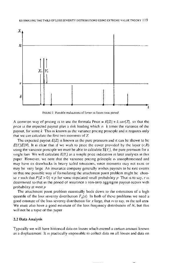
FK,u~i 2 High-excess layer m relalLOn to avaulablc data

100

ESTIMATING THE rAILS OF LOSS SEVERITY DISTRIBUTIONS USING EXTREME VALUE THEORY 121

Figure 2 shows the empirical distribution function of the Danish fire loss data evalua- ted at each of the data points. The empirical d f. for a sample of size n is defined by

Fn(x) = n - ' 2', '=. IIx, s~l ' i'e' the number of observations less than or equal to x diu-

ded by n. The einplrlcal d f. forms an approximation to the true d.f which inay be quite good in the body of the distribution; however, it is not an estimate which can be successfully extrapolated beyond the data.

The full Danish data comprise 2492 losses and can be considered as being essenti- ally all Danish fire losses over one mflhon Danish Krone (DKK) from 1980 to 1990

plus a number of smaller losses below one mllhon DKK We restrict our attention to the 2156 losses exceeding one million so that the effective displacements5 is one We work in units of one million and show the x-axis on a log scale to indicate the great range of the data

Suppose we are iequired to price a high-excess layer running from 50 to 200 In this intelval we have only six observed losses. If we fit some overall parametric severity

distribution to the whole dataset it may not be a particularly good fit in this tail area where the data are sparse

There are basically two options open to an insuralace coinpany Either it inay choo- se not to insure such a layer, because of too little experience of possible losses. Or, if it wishes to insure the layer, ~t must obtain a good estimate of the severity distribution in the tail

To solve this problem we use the extreme value methods explained m the next sec- tion. Such methods do not predict the future with certainty, but they do offer good models for explaining the extreme events we have seen m the past. These models are not arbitrary but based on rigorous matheinatical theory concerning the behavlour of extrema

3 EXTREME VALUE THEORY

In the following we summarize the results from EVT which underlie our modelling General texts on the subject of extreme values include Falk, Husler & Reiss (1994), Embrechts, Kluppelberg & Mikosch (1997) and Reiss & Thomas (1996)

3.1 The generalized extreme value d is t r ibut ion

Just as the normal distribution proves to be the nnportant hmitlng distribution for sample sums or averages, as is rnade explicit in the central hnnt theorem, another family of distributions proves important in the study of the hmltlng behavlour of sam- ple extrema. This is the famdy of extreme value distributions

This family can be subsumed under a single parametrizatlon known as the generali- zed extreme value distribution (GEV). We define the d f of the standard GEV by

J~exp(-(I + ~ , ) - " ¢ ) if ~ * O, H:(x)

" ~Lexp(-e- ) if ~ = O,

122 ALEXANDER J MC NElL

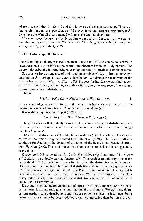
where x is such that 1 + ~ > 0 and ~ is known as the shape parameter. Three well

known distributions are specml cases, if ~ > 0 we have the Fr6chet d~stnbunon, if ~ < 0 we have the Welbull distribution; ~ = 0 gives the Gumbel dlstnbunon

If we introduce location and scale parameters/.t and cr > 0 respectively we can ex- tend the family of dls tnbunons We define the GEV H ~ o ( x ) to be H~((x - Lt)/cr) and we say that H,~ u o is of the type H e

3.2 The Fisher-Tippett Theorem

The FJsher-Tlppett theorem is the fundamental result m EVT and can be considered to have the same status in EVT as the central hmlt theorem has in the study of sums The theorem describes the hmltmg behavlour of appropriately normahzed sample maxmla.

Suppose we have a sequence of i i.d random variables X~, X 2, from an unknown

dlstnbutlon F - perhaps a loss seventy distribution. We denote the maximum of the first n observations by M, = max(Xp , X,,) Suppose further that we can find sequen- ces of real numbers a,, > 0 and b, such that (M,, - b,)/a,, the sequence of normalized maxima, converges in dlStrlbuhon

That is

P{(M, , , -b , ) /a , <x} = F"(anx + b,)---> H(x), as n--~ oo, (1)

for some non-degenerate d f H(x) If this condmon holds we say that F is m the maximum domain of attracnon of H and we wnte F ~ MDA (H)

It was shown by Fisher & Tippett (1928) that

F ~ MDA (H) ~ H is of the type H~ for some ~.

Thus, if we know that suitably normalized maxima converge in distribution, then the lnmt d ls tnbunon must be an extreme value dls tnbunon for some value of the pa- rameters ~, p and cr

The class of distributions F for which the condmon (I) holds is large A variety of eqmvalent conditions may be derived (see Falk et al. (1994)) One such result is a condition for F to be in the domain of attracnon of the heavy tailed Fr6chet distribu-

tion (H~ where ~ > 0). This is of interest to us because insurance loss data are generally heavy tailed

Gnedenko (1943) showed that for 4 > 0, F ~ MDA (H~) if and only ff 1 - F(x) = x ~/~ L(x), for some slowly varying function L(x) This result essentmlly says that ,f the tall of the d f. F(x) decays hke a power funcnon, then the d,s tnbunon is in the domain of attraction of the Fr6chet The class of d~str|bunon,, whele the tall decays hke a po-

wer function is quite large and includes the Pareto, Burr, loggamma, Cauchy and t-

distributions as well as various mixture models. We call distributions m this class heavy tailed d~stribunons, these are the dlstnbuttons which will be of most use in modelling loss severity data

Dlstrlbunons In the maximum domain of attracnon of the Gumbel MDA (Ho) inclu- de the normal, exponentml, gamma and Iognormal d,stnbunons. We call these distri-

butions medium tailed distributions and they are of some interest in insurance Some insurance datasets may be best modelled by a medium tailed d~stnbunon and even

ESI IMATING "['FIE TAILS OF LOgS SEVERITY DISTR IBUTIONS USING EX rREME VALUE THEORY 123

when we have heavy taded data we often compare them with a medium taded refe- rence &stributJon such as the exponentml in exploratwe analyses

Particular mention should be made of the Iognormal d~strlbuUon which has a much beaver tall than the normal &stnbutlon. The lognormal has historically been a popular model for loss seventy distributions; however, since it is not a member of MDA (HO for { > 0 ~t is not techmcally a heavy taded distribution

Distributions in the domain of attraction of the Welbull (H{ for ~ < 0) are short taded distributions such as the uniform and beta d~strlbut~ons. This class ~s generally of lesser interest m insurance apphcauons although ~t ~s possible to imagine s~tuat~ons where losses of a certain type have an upper bound which may never be exceeded so that the support of the loss severity d~stribunon ~s finite Under these circumstances the tad might be modelled with a short taded d~str~bunon

The Fisher-Tippet t theorem suggests the fitting of the GEV to data on sample maxima, when such data can be collected There ~s much literature on this topic (see Embrechts et a l , 1997), particularly m hydrology where the so-called annual maxima method has a long history A well-known reference is Gumbel (1958)

3.3 The generalized Pareto distribution

An equivalent set of results in EVT describe the behav~our of large observations which exceed high thresholds, and this is the theoretical formulauon which lends ~tself most readdy to the modelhng of Insurance losses This theory addresses the quesnon gwen an observation ~s extreme, how extreme might ~t be ̀ ) The &stribut~on which comes to the fore m these results Is the generahzed Pareto &stributlon (GPD)

The GPD is usually expressed as a two parameter dlStrlbuuon with d f

{ l l - ( l + ~ x / ° ' ) - I t ~ ' f ~ : 0 ' (2) G~.~(x) = - e x p ( - x / or) if ~ = 0,

where o ' > 0, and the support is x > 0 when ~ > 0 and 0 <.~ <-o"/4 when ~ < 0 The GPD again subsumes other d~Strlbuuons under its parametr~zatlon When ~ > 0 we have a reparametr~zed version of the usual Pareto distribution, if ~ < 0 we have a type II Pareto distribution, ~ = 0 gives the exponential distribution

Again we can extend the famdy by adding a location p a r a m e t e r / l The GPD G¢~,.o(x) is defined to be G~,,(x - la).

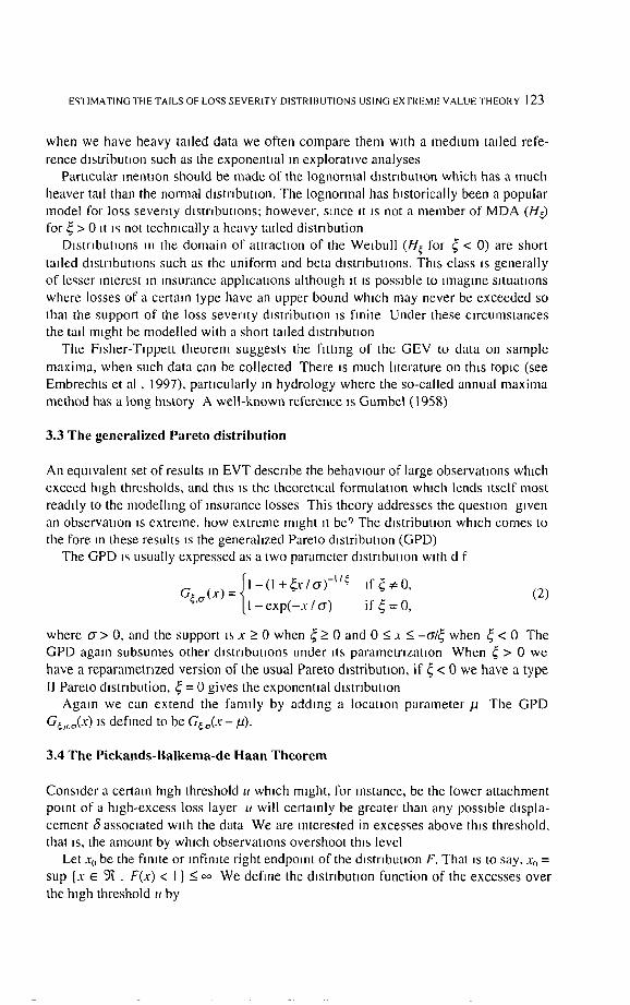
3.4 The Pickands-Balkema-de Haan Theorem

Consider a certain high threshold u which might, for instance, be the lower attachment point of a high-excess loss layer u will certainly be greater than any possible displa- cement S associated with the data We are interested in excesses above this threshold. that is, the amount by which observahons overshoot this level

Let xo be the fimte or mfimte right endpomt of the &stnbutJon F. That is to say. x 0 = sup {x 6 • . F(x) < 1 } _< ¢o We define the distribution function of the excesses over the high threshold it by

124 A L E X A N D E R J M C N E l L

F(x + u) - F(u) F,,(x)= P{X-u_< xl X > u} =

I - F ( u )

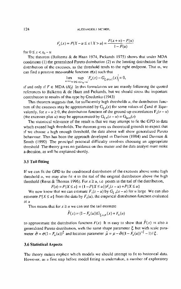
forO<_x < x o - u The theorem (Balkema & de Haan 1974, Plckands 1975) shows that under MDA

conditions (1) the generalized Pareto d~stnbution (2) ~s the hmlting dtstnbutlon for the d~stnbutlon of the excesses, as the threshold tends to the right endpolnt. That is, we can find a positive measurable function o'(u) such that

hm sup F , , (x ) - G~.,~o,)(x) = O, It'--) t 0 0 < - ~¢<j it 0 --U

if and only ff F ~ MDA (He) In this formulation we are mainly following the quoted references to Balkema & de Haan and Ptckands, but we should stress the important

contribution to results of this type by Gnedenko (1943) This theorem suggests that, for sufficiently high thresholds u, the distribution func-

tion of the excesses may be approximated by G ~ ( x ) for some values of ~and cr Equi- valently, for x - u > 0, the distribution function of the ground-up exceedances F,(x - u) (the excesses plus u) may be approximated by G~ °(x - u) = G~,, o(X)

The staust~cal relevance of the result is that we may attempt to fit the GPD to data which exceed high thresholds. The theorem gwes us theoretical grounds to expect that if we choose a high enough threshold, the data above wdl show generalized Pareto behavlour. This has been the approach developed ,n Davison (1984) and Davlson & Smith (1990) The principal practical diff iculty involves choosing an appropriate threshold The theory gives no guidance on th~s matter and the data analyst must make

a decision, as wdl be explained shortly.

3.5 Tail fitting

If we can fit the GPD to the condttlonal dlstrlbutton of the excesses above some high threshold u, we may also fit it to the tad of the original d~strlbutlon above the high threshold (Re~ss & Thomas 1996). For x > u, i.e points in the tall of the distribution,

F(x) = P { X < x} = (I - P I X < u})F,,(x- u) +P{X < u} We now know that we can estimate F,(x - u) by G¢ o(x - u) for u large We can also

estimate P{X < u} from the data by F,(u), the empirical distribution function evaluated

at u This means that for x > u we can use the tall estimate

F(x) = (1 - F,, (u))G~,,, a (x) + F,, (u)

to approximate the distribution functton F(x) It is easy to show that ~'(x) is also a

generahzed Pareto dlstribuuon, with the same shape parameter ~, but with scale para-

meter 6- = cr(l - F,,(u)) ~ and location parameter /] = # - 6 - ( 0 - F,,(u)) -# - 1)/~.

3.6 Statistical Aspects

The theory makes exphclt which models we should attempt to fit to historical data. However, as a first step before model fitting ~s undertaken, a number of exploratory

ESTIMATING THE TAILS OF LOSS SEVERITY DISTRIBUTIONS USING EXTREME VALUE THEORY ] 2 5

graphical methods provide useful preliminary infornlatlon about the data and m pan.i- cular their tall. We explain these methods m the next section in the context of an ana- lysis of the Danish data

The generalized Pareto dlstnbution can be fitted to data on excesses of high thres-

holds by a vanety of methods including the nlaxlmum likelihood method (ML) and the method of probability weighted moments (PWM) We choose to use the ML-method For a comparison of the relative merits of the methods we refer the reader to Hosklng & Walhs (1987) and Rootz6n & Tajvidl (1996).

For ~ > - 0 5 (all heavy tailed applications) it can be shown that maximum likeli- hood regularity conditions are fulfilled and that maximum likelihood esnmates

(~U,, ,~N,, ) based on a sample of N. excesses of a threshold u are asymptotically nor-

really distributed (Hosking & Walhs 1987) Specifically for a fixed threshold u we have

,v,, tON.) L to .s ' t .< : , ( l +¢ ) '

as N,, e oo. This result enables us to calculate approximate standard errors for our maximum likelihood estimates.

0

o 0

0

Q o

0 Iz3

0

030180 030182 030184 030186 030188 030190

Time

]l]]llb,,.,..__ 0t 0

6

¢q

d

0 0

1 2 3 4 5

10g(data)

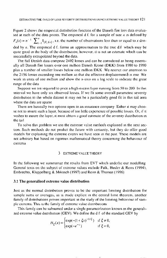
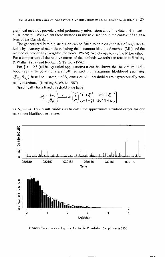
FIGURE3 Time sene~ and log data plolg for the Danish data Sample size ~s 2156

126 ALEXANDER J MC NEIL

4 ANALYSIS OF DANISH FIRE LOSS DATA

The Damsh data consist of 2156 losses over one million Danish Krone (DKK) from the years 1980 to 1990 inclusive (plus a few smaller losses which we ignore m our analyses) The loss figure is a total loss figure for the event concerned and includes damage to buildings, damage to furniture and personal property as well as loss of profits. For these analyses the data have been adjusted for Inflation to reflect 1985 values

4.1 Exploratory data analysis

The time series plot (Figure 3, top) allows us to identify the most extreme losses and their approximate t~lnes of occurrence We can also see whether there IS evidence of clustenng of large losses, which might cast doubt on our assumption of H.d data Th~s

does not appear to be the case with the Danish data The h~,~togram on the log scale (Figure 3, bottom) shows the wide range of the data

It also al lows us to see whether the data may perhaps have a lognormal right tall, which would be indicated by a familiar bell-shape m the log plot.

We have fitted a truncated lognormal distribution to the dataset using the maximum likelihood method and superimposed the resulting probabdlty density function on the

histogram. The scale of the y-ax~s is such that the total area under the curve and the total area of the histogram are both one The truncated Iognormal appears to provide a reasonable fit but it is difficult to tell from this picture whether it is a good fit to the largest losses in the high-excess area m which we are interested

The QQ-plot against the exponential distribution (Figure 4) is a very useful guide to heavy tads It examines visually the hypothesis that the losses come from an exponen-

tial distribution, ~.e from a distribution with a medium sized tall. The quantlles of the empirical distribution function on the x-ax~s are plotted against the quantdes of the exponential distribution function on the y-axis The plot is

( ( X k . , .' n - k + l = ,n}, G~, (-----~-~---11, ~ l,

where X~ ,, denotes the kth order statistic, and G -~ 0: is the inverse of the d f. of the ex-

ponentml dlstnbut,on (a special case of the GPD) The points should he approximately along a straight line if the data are an i.i.d, sample from an exponential distribution

A concave departure from the ideal shape (as in our example) indicates a heawer tailed dlstnbutlon whereas convexity indicates a shorter taded distribution. We would expect insurance losses to show heavy tailed behavlour.

The usual caveats about the QQ-plot should be mentioned. Even data generated from an exponentml distribution may sometimes show departures from typical expo- nent,al behavlour In general, the more data we have, the clearer the message of the QQ-plot. With over 2000 data points m this analysis ~t seems safe to conclude that the tad of the data ~s heavier than exponential.

ESTIMATING THE TAILS OF LOSS SEVERITY DISTRIBUTIONS USING EXTREME VALUE THEORY 1 2 7

- - ted

uJ

O )

O

QQPIot Sample Mean Excess Plot

O "

• e •

/ 0 50 1 O0 150 200 250 0 10 20 30 40 50 60

Ordered Data 'Threshold

FIC, URE4 QQ-pIoI and sample mean excess function

A further useful graphical tool is the plot o f the sample mean excess function (see

again Figure 4) which =s the plot.

{(u,e.(.)),X .... <u<Xl , ,}

where X t ,, and X,, ,, are the first and nth order s tausucs and e,,(u) is the sample mean

excess function defined by

y_."=,(x, - . r

i e. the sum of the excesses over the threshold u d~vlded by the number o f data points

which exceed the threshold u

The sample mean excess function en(u ) IS an empir ical e sumate of the mean excess

funcuon which is def ined as e(u) = E[X - u I X > u] The mean excess function descri-

bes the expected overshoot of a threshold given that exceedance occurs.

In plott ing the sample mean excess function we choose to end the plot at the fourth

order staust~c and thus omit a possible three further points, these points, being the

averages of at most three observations, may be erratic.

128 A L E X A N D E R J M C N E l L

The interpretation of the mean excess plot as explained in Beurlant, Teugels & Vynckler (1996), Embrechts et al. (1997) and Hogg & Klugman (1984). If the poants

show an upward trend, then th,s ,s a s,gn of heavy tailed behavlour. Exponentially dtstr,buted data would give an approxamately horizontal lane and data from a short tatled distribution would show a downward trend.

In particular, af the empirical plot seems to follow a reasonably straaght hne wnth positive gradtent above a certain value of u, then thts ns an mdtcatnon that the data follow a generahzed Pareto dastrtbut~on with pos]tave shape parameter an the tad area

above u Thas as precisely the kind of behavaour we observe m the Dantsh data (Fagure 4)

There as evtdence of a stra]ghtenmg out of the plot above a threshold of ten. and per-

haps again above a threshold of 20. In fact the whole plot ]s sufficiently straight to suggest that the GPD maght provade a reasonable fit to the entire dataset.

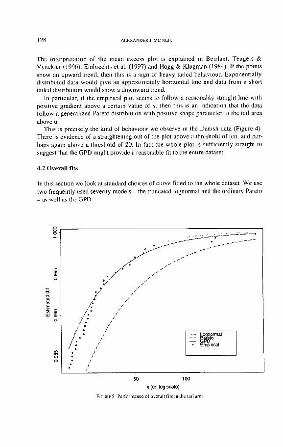
4 . 2 O v e r a l l f i t s

In thas sect,on we look at standard cho,ces of curve fitted to the whole dataset We use

two frequently used seventy models - the truncated Iognormal and the ordinary Pareto

- as well as the GPD

0

"0

o

~0 O~ 0

/ e •

' e e

/ : / ."

/.:

° . " . - - - - - " " " • e . - - - - e

1- / ~ e / . / "

J

/ • /

°,7 /

/ /

/ /

.... LoQnormal P~i~ t°

• ~mpmcal

50 1 O0

x (on log scale)

FIGURE5 Perfornmnee ot overall fits m the tall area

ESTIMATING THE TAILS OF LOSS SEVERITY DISTRIBUTIONS USING EXTREME VALUE THEORY 1 2 9

By ordmary Pareto we mean the distr ibution with d f F(x) = 1 - (abe) '~ for unknown

posi t ive parameters a and o~ and with support x > a This distribution can be rewritten

a s F ( x ) = I - ( 1 + ( x - a ) / a ) " s o t h a t t t t s s e e n t o b e a G P D w l t h s h a p e ~ = I / a , scale

= a/a and locatton Lt = a. That ts to say tt ts a G P D where the scale parameter is

cons t ramed to be the shape mul t tphed by the locatton It ts thus a little less f lexible

than a GPD wtthout thts constramt where the scale can be freely chosen.

As d iscussed earlier, the lognormal dlstr lbut ton ts not strictly speaking a heavy

tailed distribution H o w e v e r it is moderate ly heavy tailed and in many apphcatzons it is quite a good loss severity model.

In Ftgure 5 we see the fit of these models in the tall area above a threshold of 20.

The Iognormal is a reasonable fit, a l though tts tall ts just a little too thin to capture the behavlour of the very htghest observed losses. The Pareto, on the other hand, seems to

overes t imate the probabil i t ies o f large losses. Thns, at first sight, may seem a desirable,

conservat ive mode lhng feature But it may be the case, that this d f is so conservat ive ,

that tf we use tt to answer our at tachment point and premtum calculauon problems, we

wtll a m v e at answers that are unrealist ically high

O

e0 o

c.o o

~5

1.1.1

o

t%l O

GPD Fit (u =10)

o o

10 50 100

X (on 10g scale)

GPD Fit (u =20)

I

Od

O

O

50 100

X (on log scale)

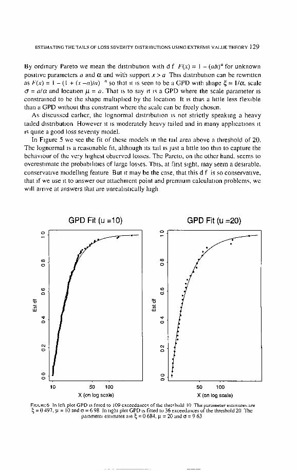
FIGURE 6 In left plot GPD Is fitted to 109 exceedances of the threshold I 0 The parameter esttmate~ are = 0 497, tU = 10 and ~ = 6 98 In nght plot GPD ts fitted to 36 exceedances of the threshold 20 The

parameter esumates are ~ = 0 684. p = 20 and ~ = 9 63

130 A L E X A N D E R ] M C N E l L

GPD Fit to Tail (u =10) 0

0

(D 0

0

o4 o

0 d

5 10 50 100

X (on log scale)

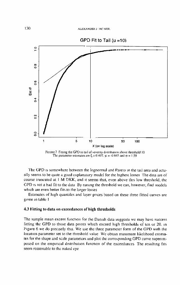
FIGURE 7 Fatmg the GPD to tall of seventy d]stnbutton above threshold 10 The parameter estimates are ~ = 0 497, ~ = -0 845 and c = I 59

The GPD ~s somewhere between the lognormal and Pareto m the tall area and actu-

ally seems to be qmte a good explanatory model for the highest losses The data are of

course truncated at I M DKK, and ~t seems that, even above th,s low threshold, the

GPD is not a bad fit to the data By raising the threshold we can, however , find models which are even better fits to the larger losses

Estmlates o f h~gh quantt les and layer prices based on these three fitted curves are gwen m table I

4.3 Fitting to data on exceedances of high thresholds

The sample mean excess function for the Damsh data suggests we may have success

fit t ing the G P D to those data points which exceed high thresholds of ten or 20, m

Figure 6 we do precisely this. We use the three parameter form of the GPD with the

location parameter set to the threshold value We obtain max imum hkehhood eshma-

tes for the shape and scale parameters and plot the corresponding GPD curve supen m-

posed on the empir ica l dis tr ibut ion funct ion o f the exceedances The resul tmg fits

seem reasonable to the naked eye

ESTIMA FING THE TAILS OF LOSS SEVERITY DISTRIBUTIONS USING EXTREME VALUE THEORY l 31

if)

C)

o~ O II

t~ CO

0 d

Threshold

314 3.30 3.50 377 3.99 417 450 487 5.38 5.79 6.67 799 108014.302200 i i [ i i i i i i ~ i i i i i i i i i i i i i i i i i

. . . ° .

, , , , , , , , , , , ~ , , , , , , , , , , ,

500 466 433 399 366 332 299 265 232 198 165 132

Number of exceedances

98 81 65 48 31 15

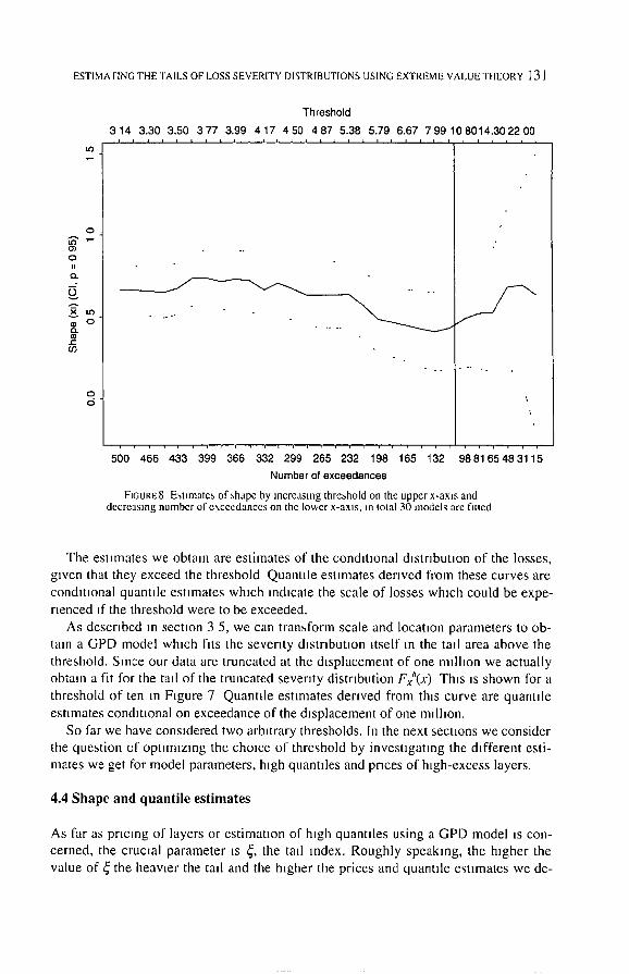
FIGURE8 Esumates of,shape by increasing threbhold on the upper x-axm and decreas ing number of e \ c e e d a n c e s on the lower x-axm, m Iolal 30 models are fiued

The esmnates we obtain are estitnates of the conditional dmtrlbutlon of the losses, given that they exceed the threshold Quantlle estimates derived from these curves are condmonal quantlle estimates which indicate the scale of losses which could be expe- rienced ff the threshold were to be exceeded.

As described in section 3 5, we can transform scale and location parameters to ob- tain a GPD model which fits the seventy dls tnbuuon itself in the tad area above the threshold. Since our data are truncated at the displacement of one million we actually obtain a fit for the tall of the truncated seventy distribution Fxa(X) This is shown for a threshold of ten in Figure 7 Quantde estimates derived from this curve are quantlle estimates condmonal on exceedance of the displacement of one indhon.

So far we have considered two arbHrary thresholds, in the next secuons we consider the question of optHnlzlng the choice of threshold by investigating the different esti- mates we get for model parameters, high quantlles and prices of high-excess layers.

4.4 Shape and quantile estimates

As far as pricing of layers or estimation of high quantfles using a GPD model is con- cerned, the crucml parameter is ~, the tall ,ndex. Roughly speaking, the higher the value of ~ the heavier the tall and the higher the prices and quantde estimates we de-

132 ALEXANDERJ MCNEIL

o

o Q 03

o 03

314 3.30 3.50 377 399 417 450 4.87 538 579 6.67 7.99108014.302200

f

500 466 433 399 366 332 299 265 232 198 165 132 988165483115

Number of exceedances

U3

O

0

0

0

0

0

314 3.30 350 3.77 3.99 417 450 487 538 579 667 7 9 9 1 0 8 0 1 4 3 0 2 2 0 0

\ f

500 466 433 399 366 332 299 265 232 198 165 132 988165483115

Number of exceedances

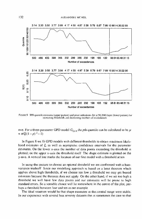
I=IGURE9 999 quantde esnmates (upper picture) and price md~c,'mom, for a (50,200) layer (lower picture) Ior increasing thresholds and decreasing numbers of exceedances

rive. For a three-parameter GPD model G~u o the pth quantile can be calculated to be u + o-/~((I - p ) ~ - 1)

In Figure 8 we fit GPD models with different thresholds to obtain maximum hkell-

hood estimates of ~, as well as asymptouc confidence intervals for the parameter

esUmates. On the lower x-axis the number of data points exceeding the threshold is

plotted; on the upper x-axis the threshold itself The shape estimate is plotted on the

y-ax~s. A vertical hne marks the locaUon of our first model with a threshold at ten

In using this picture to choose an optimal threshold we are confronted with a bias-

variance tradeoff Since our modelling approach is based on a hmlt theorem which

applies above high thresholds, if we choose too low a threshold we may get bmsed

estimates because the theorem does not apply On the other hand, if we set too high a

threshold we wall have few data points and our estimates will be prone to high

standard errors. So a sensible choice wall lie somewhere in the centre of the plot, per-

haps a threshold between four and ten in our example

The ideal s~tuauon would be that shape esumates in this central range were stable.

In our experience with several loss severity datasets this is sometimes the case so that

ESTIMATING THE TAILS OF LOSS SEVERITY I)[S'I'R[BU I'IONS USING EX'I REME VALUE TIIEORY 1 3 3

the data conform very well to a particular generalized Pareto distribution in the tall

and inference ~s not too sensitive to choice of threshold. In our present example the

shape estimates vary somewhat and to choose a threshold we should conduct further

i n v e s t i g a t i o n s .

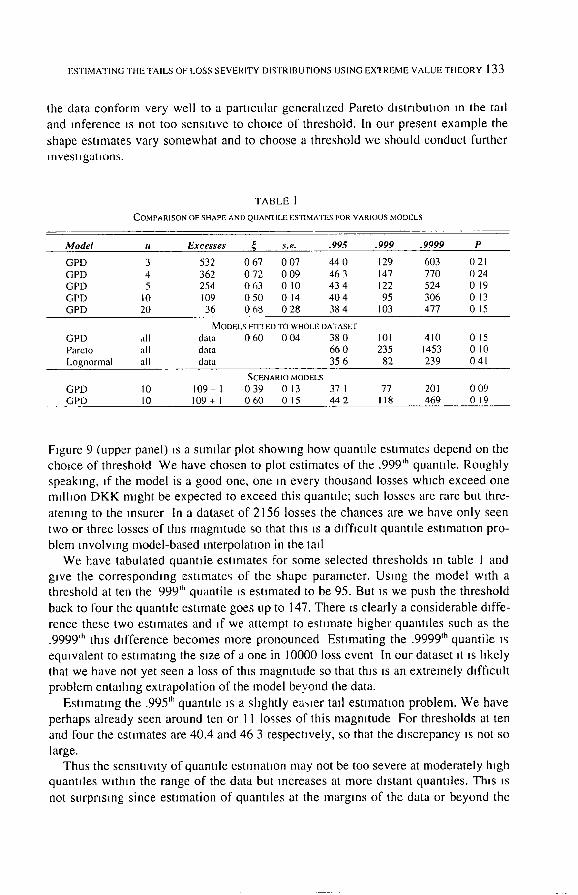
T A B L E I

COMPARISON OF SHAPE AND QUAN'I ILE ESTIMATES FOR VARIOUS MODELS

Model u Excesses ~ s.e. .995 .999 .9999 P

GPD 3 532 0 67 0 07 44 0 129 603 0 21 GPD 4 362 0 72 0 09 46 3 147 770 0 24 GPD 5 254 0 6 3 0 10 4 3 4 122 524 0 19 GPD 10 109 0 5 0 0 14 4 0 4 95 306 0 13 GPD 20 36 0 6 8 0 2 8 3 8 4 103 477 0 15

MODELS FIT1ED TO WHOLE DATASET GPD all data 0 6 0 0 0 4 3 8 0 101 410 0 15 ParcIo all data 66 0 235 1453 0 10 Lognormal all data 35 6 82 239 0 41

SCENARIO MODELS GPD 10 1 0 9 - I 0 3 9 0 13 37 I 77 201 0 0 9 GPD 10 109+ I 0 6 0 0 1 5 4 4 2 118 469 0 1 9

Figure 9 (upper panel) is a similar plot showing how quantlle estimates depend on the choice of threshold We have chosen to plot estimates of the .999 'h quantlle. Roughly speaking, if the model is a good one, one in every thousand losses which exceed one million DKK might be expected to exceed this quantlle; such losses are rare but thre-

atening to the insurer In a dataset of 2156 losses the chances are we have only seen two or three losses of this magnitude so that this is a difficult quantlle estimation pro- blem involving model-based interpolation in the tall

We have tabulated quantlle estimates for some selected thresholds in table I and give the corresponding estimates of the shape parameter. Using the model with a threshold at ten the 999 I" quantile IS estimated to be 95. But is we push the threshold back to four the quantlle estimate goes up to 147. There is clearly a considerable diffe- rence these two estimates and if we attempt to estimate higher quantlles such as the .9999 'h this difference becomes more pronounced Estimating the .9999'" quantile is equivalent to estimating the size of a one in 10000 loss event In our dataset it is likely that we have not yet seen a loss of this magmtude so that this is an extremely difficult problem entalhng extrapolation of the model beyond the data.

Estimating the .995 t" quantlle is a slightly caller tall estimation problem. We have perhaps already seen around ten or 1 I losses of this magnitude For thresholds at ten and four the estimates are 40.4 and 46 3 respectively, so that the discrepancy is not so

large. Thus the sensitivity of quantlle estimation may not be too severe at moderately high

quantlles wtthln the range of the data but increases at more distant quantlles. This is

not surprising since estimation of quantlles at the margins of the data or beyond the

134 ALEXANDER J MC NElL

data is an inherently difficult problem which represents a challenge for any method. It should be noted that although the estimates obtained by the GPD method often span a wide range, the estimates obtained by the naive method of fitting ordinary Pareto or lognormal to the whole dataset are even more extreme (see table) To our knowledge the GPD estimates are as good as we can get using parametric models

4.5 Calculating price indications

In considering the issue of the best choice of threshold we can also investigate how price of a layer varies with threshold To give an indication of the prices we get from our model we calculate P -- ElF, I X, > ~] for a layer running from 50 to 200 nnlhon (as in Figure 2) It is easily seen that, for a general layer (r. R), P is given by

P = ~ x - r)fx, (x)cL~ + ( R - r)(I - Fx~ (R)), (3)

where fx6(X) = dFxS(x)/dx denotes the density function for the losses truncated at Picking a high threshold u (< r) and fitting a GPD model to the excesses, we can esti- mate Fx6(x) forx > u using the tail esumation procedure We have the estimate

~x~ (x) = (I - F,, (u))G~.,,.,~ (x) + F,, (u),

where ~ and 6" are maximum-hkehhood parameter estimates and F,(u) is an estimate

of P{X ~<_ u} based on the empirical distribution function of the data We can estimate the density function of the 6-truncated losses using the derivative of the above expres-

sion and the integral in (3) has an easy closed form In Figure 9 (lower picture) we show the dependence of P on the choice of threshold

The plot seems to show very smnlar behavlour to that of the 999 'h percentile estimate, with low thresholds leading to higher prices The question of which threshold is ulti- mately best depends on the use to which the results are to be put If we are trying to answer the optimal attachment point problem or to price a high layer we may want to

err on the side of conservatism and arrwe at answers which are too high rather than too low. In the case of the Danish data we might set a threshold lower than ten, per- haps at four The GPD model may not fit the data quite so well above this lower thres- hold as it does above the high threshold of ten, but it might be safer to use the low threshold to make calculations

On the other hand there may be business reasons for trying to keep the attachment

point or premium low. There may be competition to sell high excess policies and this may mean that basing calculations only on the highest observed losses is favoured, since this will lead to more attractive products (as well as a better fitting model)

In other insurance datasets the effect of varying the threshold may be different In- ference about quantdes might be quite robust to changes in threshold or elevation of the threshold might result m higher quantde estimates Every dataset is unique and the

data analyst must consider what the data mean at every step The process cannot and should not be fully automated

ESTIMATING THE TAILS OF LOSS SEVERITY DISTRIBUTIONS USING EXTREME VALUE THEORY ] 3 5

4.6 Sensitivity of Results to the Data

We have seen that inference about the tall of the severity distribution may be sensitive to the choice of threshold It is also sensitive to the largest losses we have m our data- set. We show this by consldermg two scenarios m Table I.

In the first scenario we remove the largest observation from the dataset. If we return to our first model with a threshold at ten we now have only 108 exceedances and the estimate of the .999 'h quantlle is reduced from 95 to 77 whilst the shape parameter falls

from 0.50 to 0 39 Thus omission of this data point has a profound effect on the esh- mated quantlles. The estimates of the .999 'h and 9999 'h quantiles are now smaller than any previous estimates

In the second scenario we introduce a new largest loss of 350 to the dataset (the previous largest be,ng 263) The shape estimate goes up to 0.60 and the eStllnate of the 999 "~ quantlle increases to 118 Th,s is also a large change, although m this case it is

not as severe as the change caused by leaving the dataset unchanged and reducing the threshold from ten to five or four

The message of these two scenarios is that we should be careful to check the ac-

curacy of the largest data points in a dataset and we should be careful that no large data points are deemed to be outhers and omitted if we wish to make inference about the tall of a distribution. Addmg or deletmg losses of lower magnitude from the data-

set has much less effect

5 . DISCUSSION

We hope to have shown that fitting the generalized Pareto distribution to msurance losses which exceed high thresholds is a useful method for estimating the tails of loss severity dlstrlbut,ons In our experience with several msurance datasets we have found consistently that the generahzed Pareto distribution ~s a good approximation m the tall

This Is not altogether surpr~smg As we have explained, the method has solid foun-

dations in the mathematical theory of the behaviour of extremes; it is not simply a question of ad hoc curve fitting It may well be that, by trial and error, some other distribution can be found which fits the avadable data even better in the tall But such a distribution would be an arbitrary choice, and we would have less confidence m extrapolating it beyond the data

It is our belief that any practitioner who routinely fits curves to loss severity data

should know about extreme value methods There are, however, an number of caveats to our endolsement of these methods We should be aware of various layers of uncer- tamty which are present m any data analysis, but which are perhaps magmfied m an extreme value analys~s

On one level, there is parameter uncertainty. Even when we have abundant, good- quality data to work with and a good model, our parameter estlmales are still subject

to a standard error We obtain a range of parameter estimates which are compatible w~th our assumptions As we have already noted, inference is sensitive to small chan- ges m the parameters, particularly the shape parameter

136 ALEXANDER J MC NElL

Model uncertainty ~s also present - we may have good data but a poor model. Using extreme value methods we are at least working with a good class of models, but they are apphcable over h~gh thresholds and we must decide where to set the threshold If

we set the threshold too high we have few data and we introduce more parameter uncertainty If we set the threshold too low we lose our theoretical jusuficauon for the model. In the analysis presented m th~s paper inference was very sensmve to the thres- hold choice (although this is not always the case).

Equally as serious as parameter and model uncertainty may be data uncertainty. In a sense, it is never possible to have enough data m an extreme value analysis Whilst a

sample of 1000 data points may be ample to make reference about the mean of a dls- tnbuuon using the central hm~t theorem, our inference about the tad of the distnbuuon is less certain, since only a few points enter the tad region. As we have seen, inference is very sensitive to the largest observed losses and the mtroductton of new extreme losses to the dataset may have a substantial mapact For this reason, there may still be a role for stress scenarios in loss severity analyses, whereby historical loss data are

enriched by hypothetical losses Io investigate the consequences of unobserved, adver- se events

Another aspect of data uncertainly ts that of dependent data. In this paper we have made the fanuhar assumption of independent, identically d~stnbuted data In practice we may be confronted with clustering, trends, seasonal effects and other kinds of de- pendencies. When we consider fire losses m Denmark it may seem a plausible first

assumption that individual losses are independent of one another, however, it is also possible to imagine that circumstances conducive or mhlbmve to fire outbreaks gene- rate dependenctes m observed losses. Destructive fires may be greatly more common m the summer months, buildings of a particular wntage and building standard may succumb easdy to fires and cause h~gh losses Even after ajustment for inflation there may be a general trend of increasing or decreasing losses over time, due to an increa-

sing number of increasingly large and expensive buddmgs, or due to increasingly good safety measures

These issues lead to a number of interesting stausucal questions in what is very much an active research area. Papers by Davlson (1984) and Davlson & Smith (1990) discuss clustering and seasonahty problems m environmental data and make suggesti- ons concerning the modelhng of trends using regression models built into the extreme

value modelhng framework The modelhng of trends is also discussed m Rootz6n & Tajvldl (1996).

We have developed software to fit the generahzed Pareto dls tnbuuon to exceedan- ces of high thresholds and to produce the kinds of graphical output presented in this paper It ~s wnten m Splus and ~s available over the World Wide Web at http://www math ethz ch/~mcned

ESTIMATING THE TAILS OF LOSS SEVERITY DISTRIBUTIONS USING EXTREME VALUE THEORY 137

6 ACKNOWLEDGMENTS

Much of the work in this paper came about through a collaborative project with Swiss Re Zurich. I gratefully acknowledge Swiss Re for their financial support and many fruitful discussions ~

I thank Mette Rytgaard of Copenhagen Re for makmg the Danish fire loss data available and Richard Smith for advice on software and algorithms for fitting the GPD to data I thank an anonymous reviewer for helpful comments on an earlier version of

this paper Special thanks are due to Paul Embrechts for introducing me to the theory of ex-

tremes and its many lnterestmg apphcat~ons.

REFERENCES

BALKEMA, A and DE HAAN, L (1974), 'Residual hfe ume at great age'. Annal~ of Piobablht~. 2, 792-804 BEIRLANT, J and TEUGELS, J (1992), 'Modelling large clanns m non-hfe insurance'. Insurance Mathema-

tics and Economics, I t , 17-29 BEIRLANT. J . TEUGELS, J and VYNCKIER, P (1996), Practwal anaIvvl$ oJ eatreme vahte~. Leuven Umverstty

Press, Leuven D^V]SON, A (1984), Modelling excesses over high thresholds, with an apphcauon, in J de Ohve]ra. ed,

"Stausucal Extrcmcs and ApphcatJons', D Re~del, 461-482 DAVtSON, A and St, rUTH, R (1990), 'Modcls for exceedances over high thresholds (with discussion)', Jottt-

hal of the Royal Statistical Society. Series B, 52, 393-442 DE HAAN, L (1990), 'Fighting the arcil-enemy with mathenmt~cs', Statt~ttca Neerlandtca, 44, 45-68 EMBRECHTS, P. KLUPPELBERG, C (1983). 'Some awects of itt~tttatl£e mathematlc~ '. Theory of Probablhty

and its Apphcauon~ 38, 262-295 EMBRECIITS. P, KLUPPELBERG, C and MIKOSCH, T (1997), Modelhng eatremal event3 for insurance and

finance. Springer Verlag, Berhn To appear FALK, M , HUqLER, J and REI'qS, R (1994), /.ztw~ of Small nuolberv eroemes and rate events. Btrkhauser,

Basel FISHER, R and TH,PEr'r, L (1928). 'Lmmmg forn~s of the frequency dlstribuuon of the largest or smallest

member of a sample', Proceedings of the Combrtdge Philosophical Soctet 3, 24, 180-190 GNEDENKO, B (1943), 'Sur la distribution lumte du terme maxmlum d'une sEne alealolre', Atzttal9 of Mct-

thematt(s, 44, 423-453 GUMBEL. E (1958). Statistics of Eatteme~, Columbia Umvcrslty Press. New York HOGG. R and KLUGMAN, S (1984), bg~ Dtrtrtht~tlonx Wdey, New York HOSKING, J and WALLIS, J (1987), 'Parameter and quanule estm~auon for the generahzed Pareto distnbu-

uon', Technootetttcs, 29, 339-349 PICKANDS, J (1975), 'Statistical reference using extreme order statistics', The Annal~ of Statistics 3, 119-

131 REISS. R and TIIOMAS, M (1996), 'Staust~cal analysis of extreme wdue'.,' Documentation for XTREMES

software package ROOTZ~N, H and TAJVIDI, N (1996), 'Extreme value statistics and wind storm losses a casc study' To

appear m Scandmavmn Actuarml Journal SMI FII, R (1989), 'Extreme value analy~,ls of cnvlronmental time series an apphcauon to trend detecuon m

ground-level ozone', Statistical Science, 4. 367-393

I The author is supported by Swiss Re as a research fellow at ETH Zurich