Munich Personal RePEc Archive

ESTIMATING THE TOURISM

POTENTIAL IN NAMIBIA

Eita, Joel Hinaunye and Jordaan, Andre C.

15 October 2007

Online at https://mpra.ub.uni-muenchen.de/5788/

MPRA Paper No. 5788, posted 16 Nov 2007 19:53 UTC

1

ESTIMATING THE TOURISM POTENTIAL IN NAMIBIA

Joel Hinaunye Eita1 and Andre C. Jordaan

2

October 2007

Abstract

This paper investigates the determinants of tourism in Namibia for the period 1996 to

2005. The results indicate that an increase in trading partners’ income, depreciation of the

exchange rate, improvement in Namibia’s infrastructure, sharing a border with Namibia

are associated with an increase in tourist arrivals. The results show that there is

unexploited tourism potential from Angola, Austria, Botswana, Germany, South Africa

and the United States of America. This suggests that it is important to exploit the tourism

potential as this would help to accelerate economic growth and generate the much needed

employment.

JEL classification: F170, C500, C230, C330, C590

Keywords: tourism potential, panel data, fixed effects

1 Namibian Economic Policy Research Unit (NEPRU), P.O. Box 40710, WINDHOEK, Namibia, Tel: +264 61 277500, cell: +264 61 813567380. Email: hinaeita@yahoo.co.uk. 2 Investment and Trade Policy Centre, Department of Economics, University of Pretoria, 0002 PRETORIA. Tel: +2712 420 2413, Fax: +27 12 362 5207. Email: andre.jordaan@up.ac.za

2

1. Introduction

Tourism is the largest export earner in the world as it generates foreign exchange that

exceed those from products such as petroleum, motor vehicles, textiles and

telecommunication equipment since the late nineties. Giacomelli (2006) and Eilat and

Einav (2004) indicate that tourism is a labour intensive industry. It employs about 100

million people around the world and this account for 8.3 percent of world employment.

The World Travel and Tourism Council (WTTC) indicate that in 2005 tourism accounted

for about 10 percent of world GDP. Tourism is important in economies as it generates

revenues required to finance infrastructure and other projects that promote economic

development. It also promotes international peace through the provision of incentives for

peacekeeping and closure of the gap between different cultures.

The WTTC estimates that tourism accounts for a significant proportion of the GDP and

employment of developing countries and this indicates that it is important for economic

development. According to WTTC (2006) the direct impact of tourism in the Namibian

economy in 2006 is estimated at 3.7 percent of GDP and 4.7 percent of total employment.

Since tourism touches all sectors of the economy its real impact is higher. The total direct

and indirect impact of tourism is that it accounts for 17.7 percent of total employment and

16 percent of total GDP. The sector also accounts of 21 percent of the total exports of

goods and services.

3

Before and after independence in 1990, Namibia has depended on the extraction of

mineral resources, agriculture and fishing for growth and development but high

unemployment remains a challenge facing the government. The tourism sector is now

regarded as the sector with real opportunities for employment creation and economic

growth. The government of Namibia recognises the role of tourism in the economy and

has recently identified it in Vision 2030 and the National Development Plans as a priority

sector. Vision 2030 is a long-term national development framework reflecting the

aspirations and objectives of the people of Namibia. The kernel of this is the desire to

enhance the standard of living and improve the quality of life of the Namibian people.

Vision 2030 calls for every Namibian to have the standard of living equal to those in the

developed world. The development of the tourism sector is regarded as the key factor in

the Broad Based Economic empowerment. Given its importance and role in the Namibian

economy, it is important to investigate factors that determine tourism in Namibia. This

will help to analyse if there is unexploited tourism potential among Namibia’s trading

partners. An econometric model is a useful tool in analysing tourism.

In light of the above discussion, the objective of this paper is to investigate factors which

determine tourist arrivals in Namibia using an econometric model of international

tourism. It then investigates whether there is unexploited tourism potential among

Namibia’s trading partners in this sector. The rest of the paper is organised as follows.

Section 2 discusses the overview of tourism in Namibia. Section 3 discusses the literature

and model. Section 4 discusses the methodology for estimation and Section 5 provides

4

univariate characteristics of the data. Section 6 presents the estimation results, while

Section 7 discusses the tourism potential. The conclusion is presented in Section 8.

2. Overview of Tourism in Namibia

Namibia experienced a boom in the tourism sector between 1996 and 2005. The total

number of tourist arrivals in Namibia between 1996 and 2005 is presented in Figure 1.

Tourist arrivals in Namibia increased from 461310 in 1996 to 777890 in 2005.

Insert Figure 1. here

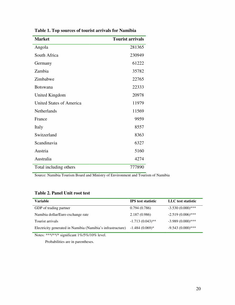
The composition of tourist arrivals in Namibia is presented in Table 1 and shows that

African countries are the main source of tourists to Namibia. With the exception of

Germany in third place in Namibia’s overall tourist ranking, African countries occupy the

top six positions. Angola and South Africa are leading source tourists for Namibia. Other

European countries (United Kingdom, Netherlands, France, Italy, Switzerland,

Scandinavia, and Austria) also account for a significant amount of tourist arrivals in

Namibia. The United States of America is the seventh main source of tourists for

Namibia.

Insert Table 1 here

5

According to the WTTC (2006), travel and tourism in Namibia is estimated to directly

produce N$ (Namibia dollars) 1.6 billion or US$256.7 million and this is equivalent to

3.7 percent of the GDP in 2006. The broader travel and tourism (which include direct and

indirect impact) is estimated to contribute N$ 6.8 billion or US$ 1.1 billion and this

accounts for 16 percent of Namibia’s GDP. The broader tourism and travel is also

expected to generate about 71800 jobs (total of direct and indirect) in 2006. This

represents 17.9 percent of the total employment in Namibia.

WTTC (2006) indicated that the travel and tourism sector plays an important role in

generating foreign exchange. It is estimated that this sector contributed N$4.4 billion or

US$715.9 million in 2006. This accounts for 21 percent of total exports of goods and

services in Namibia.

3. Literature and the Model

There are two main groups of literature on the tourism industry. The first is international

trade, which according to Eilat and Einav (2004) is a starting point because tourism is

part of international trade. The second group is the empirical tourism literature.

The general starting point for theoretical and empirical literature on international trade is

the Heckscher-Ohlin theory or pattern. It states that international trade depends on the

relative factor endowments. This is important when factors of production are capital and

labour as this makes it less necessary for tourism analysis. In the case of tourism, the

6

most important factors of production are unique to the specific country and not easy to

measure, evaluate or compute. Eilat and Einav (2004) gave examples of the Eiffel Tower,

Pyramids and nice beaches. In Namibia, sand dunes of the Namib Desert are good

examples of these unique factors of production, and it makes the investigation of the

determinants of international tourists to the country less attractive theoretically. The

ability of unique factors of production such as Sand Dunes of the Namib Desert to attract

tourists to Namibia is best measured by the number of international visitors who visit

them. An investigation of the variables that have an impact on the demand for tourism is

very important when dealing with this sector of the economy. The variables that have an

effect on tourism will be discussed later in this paper.

There are two groups in the empirical literature of tourism. The first group comprises of

studies that use time series and cointegration econometric techniques to investigate the

determinants of tourism demand and forecast the future tourist arrivals (among others,

Katafono and Gounder, 2004; Narajan, 2005; Durbarry, 2002; Divisekera, 2003; Cheung

and Law, 2001). The second group involves studies that deal with determinants of

tourism using panel data econometric techniques (such as Eilat and Einav, 2004; Luzzi

and Flückiger, 2003; Walsh, 1997; Roselló et al. 2005; Naude and Saayman, 2004). This

current study falls within the second group of the empirical tourism literature. Following

the review of the second group of the empirical tourism literature and theory, the demand

for tourism from country i to country j is specified as:

),,,,,,( ijjiijijijij AINFRAINFRATCERPYfT = (1)

7

where ijT is the number of tourist arrivals in country i from country j, jY is the income of

country j, iP is price or cost of living in country i, ijER is the exchange rate measured as

units of country i’s currency per unit of country j’s currency, ijTC is the transport costs

between country i and country j, iINFRA and jINFRA are the measure of infrastructure

in country i and j, and ijA represents any other factor that determines the arrival of

tourists from country i to country j. Equation (1) is specified in log form as for estimation

purpose as:

ijijj

iijijijij

AINFRA

INFRATCERPYT

εγγ

γγγγγγ

+++

+++++=

lnln

lnlnlnlnlnln

76

543210 (2)

The income of the source of tourism country is the most widely used variable. As Lim

(1997) states, travelling to another country is generally expensive and is regarded as a

luxury good and therefore disposable income is an appropriate variable as it affects the

ability of tourists to travel. Since disposable income data are hard to find, many studies

uses real GDP per capita, nominal or real GDP or GNP. This study uses GDP of the

tourism country as a proxy for income. An increase in income is positively related to the

number of tourist arrivals, and hence 1γ is expected to be positive.

The price of tourism is another most commonly used explanatory variable for tourism

arrivals in many studies (such as Naude and Saayman, 2004; Katafono and Gounder,

2004; Walsh, 1997; Luzzi and Flückiger, 2003). It is the cost of tourism services which

8

tourists pay at their destinations. A tourist price index which comprises of goods

purchased by tourists is appropriate, but since this index is not available, most studies use

the consumer price index as a proxy for price of tourism services. A rise in price at

destination means that the cost of tourism service is increasing and this discourages

tourist arrivals ( 2γ < 0).

The exchange rate variable is added to the list of explanatory variables in addition to the

price. This is the nominal exchange rate defined as the currency of the tourist destination

country per currency of tourist source country. A depreciation of the exchange rate makes

tourism goods and services cheaper and encourages tourist arrivals ( 3γ >0).

The cost of transport between the source and destination countries can be an important

part of the cost of tourism goods and services. According to Luzzi and Flückiger (2003),

the cost of transport should take into account the costs of an air ticket and the cost of the

whole journey. The cost of transport should comprise all components of costs to the

destination. The cost of transport to the destination could probably be measured as

weighted average price of air, sea and land. It is difficult to get data on all components of

transport costs between the source and destination countries, and most studies have used

distance in kilometres between the tourism source and tourism destination countries. This

current study also uses distance in kilometres between the source and destination

countries as a proxy for transport costs. An increase in transport costs causes a decrease

in the number of tourist arrivals, and this means that 4γ < 0.

9

A measure of infrastructure variable was added in recent research to explain tourism

flows. Studies such as Naude and Saayman (2004) used the number of hotel rooms in the

country as an indicator of tourism infrastructure. The number of hotel rooms available in

the country is an appropriate indicator of the capacity of the tourism sector in the country.

According to Naude and Sayman, the higher the number of rooms the greater the capacity

of the tourism sector and this implies that the country is highly competitive. The other

measure of infrastructure used by Naude and Sayman is the number of telephone lines per

employees. An increase or improvement in infrastructure in both the destination and

source countries attracts the number of tourist arrivals, hence 5γ and 6γ >0.

This study introduced a dummy variable to represent countries that border Namibia. After

introducing the dummy variables, Equation (2) is re-specified as:

ijj

iijijijij

BORDERINFRA

INFRADISERPYT

εγγ

γγγγγγ

+++

+++++=

76

543210

ln

lnlnlnlnlnln (3)

where ijDIS is the distance in kilometres between Namibia and its trading partners and is

a proxy for transport costs. Countries which border Namibia are given the value of 1 and

0 for otherwise. It is expected that being a neighbour to Namibia is associated with an

increase in tourist arrivals. That means the coefficient of 7γ is expected to be positive.

10

4. Estimation Procedure

There are different models in panel data estimation and these are pooled, fixed and

random effects. The pooled model assumes that countries are homogeneous, while fixed

and random effects introduce heterogeneity in the estimation. A decision should be made

whether to use random or fixed model because individual effects are included in the

regression. A random effects model is appropriate when estimating the model between a

country and its randomly selected sample of trading partners from a large group

(population). A fixed effects model is appropriate when estimating the model between a

country and predetermined selection of trading partners (Egger, 2000). Since this study

deals with tourism arrivals in Namibia from 11 selected trading partners in the tourism

sector, the fixed effects model will be more appropriate than the random effects model.

The top 11 trading partners were selected based on the tourism data for the period 1996 to

2005. In addition, the study uses the Hausman test to check whether fixed effects is more

appropriate than the random effects model. The fixed effects model will be better than the

random effects model if the null hypothesis of no correlation between individual effects

and the regressors is rejected.

The fixed effects model cannot directly estimate variables that do not change over time

because inherent transformation wipes out such variables. Martinez-Zarzoso and Nowak-

Lehmann (2001) suggested that these variables can be estimated in the second step by

running another regression with individual effects as a dependent variable and the

dummies as explanatory variables. This is estimated as:

11

iijij BORDERDISIE εγγγ +++= 210 (4)

where ijIE is individual effects.

5. Univariate Characteristics of the Variables

The study uses annual data and the estimation covers the period 1996 to 2005. Detailed

data description and their sources are given in the Appendix. Before estimating Equation

(3), univariate characteristics of the data are analysed and this involves panel data unit

root tests. Testing for unit root is the first step in determining a potentially cointegrated

relationship between variables. If all variables do not contain a unit root, the traditional

estimation methods can be used to estimate the relationship between variables. If

variables are nonstationary, a test for cointegration is required. The literature identifies

three types of unit root tests. The first test is Levin, Lin and Chu (2002) and it is referred

to as the LLC test. The second test is that of Hadri (2000). These two types of panel unit

root test assume that the autoregressive parameters are common across cross-sections.

The LLC uses the null hypothesis of a unit root while Hadri uses the null hypothesis of

no unit root.

Im, Pesaran and Shin (2003) developed a third type of panel unit root test called IPS. This

test allows for autoregressive parameters to differ across cross-sections and also for

individual unit root processes. It is computed by combining individual cross-section unit

root tests in order to come up with a test that is specific to the panel. This test has more

power than the single-equation Augmented Dickey-Fuller (ADF) by averaging N

12

independent regressions (Strauss and Yigit, 2003). The ADF specification may include

intercept but no trend or may include an intercept and time trend. It uses the null

hypothesis that all series have a unit root and the alternative hypothesis is that at least one

series in the panel has a unit root. This test is one-tailed or lower tailed based on the

normal distribution. This study uses LLC and the IPS to test for unit root. The results for

unit root test are presented in Table 2. According to the IPS test statistic only tourist

arrivals and electricity generated in Namibia are stationary and the remaining variables

are not stationary. However, the LLC indicates that the null of the unit root is rejected for

all variables, meaning that all variables are stationary. This study uses at least one test to

assume a verdict of stationarity. Since all variables are stationary, traditional estimation

techniques can be used to estimate Equation (3) and the test for cointegration is not

required.

Insert Table 2 here

6. Estimation Results

The results for the pooled, fixed effects and random effects models are presented in Table

3. The results in the second Column are those of the pooled model. The pooled model

assumes that there is no heterogeneity among countries and no fixed effects are

estimated. It therefore assumes homogeneity for all countries. It is a restricted model

because it assumes that the intercept and other parameters are the same across all trading

partners.

13

The results of the fixed effects model are in the third Column. The fixed effects model

assumes that countries are not homogeneous, and introduces heterogeneity by estimating

country specific effects. It is an unrestricted model as it allows for an intercept and other

parameters to vary across trading partners. The F-test is performed to test for

homogeneity or poolability of countries. It rejects homogeneity of countries even at 1

percent significance level and this means that a model with individual effects must be

selected.

The results of the random effects model are in Column 4. This model also acknowledges

heterogeneity among countries, but it differs from the fixed effects model because it

assumes that the effects are generated by a specific distribution. It does not explicitly

model each effect, and this avoids the loss of degrees of freedom which happens in the

fixed effects model. The LM test is applied to the null hypothesis of no heterogeneity.

The LM test also rejects the null hypothesis of no heterogeneity in favour of random

specification.

In order to discriminate between fixed effects and random effects models, the Hausman

specification test is used to test the null hypothesis that the regressors and individual

effects are not correlated. If the null hypothesis is rejected the fixed effects model will be

the appropriate model. Failure to reject the null hypothesis means that the random effects

model will be the preferred. The Hausman test rejects the null hypothesis and this

14

indicates that country specific effects are correlated with regressors and suggests that the

fixed effects model is appropriate. The random effects model will be inconsistent.

Insert Table 3 here

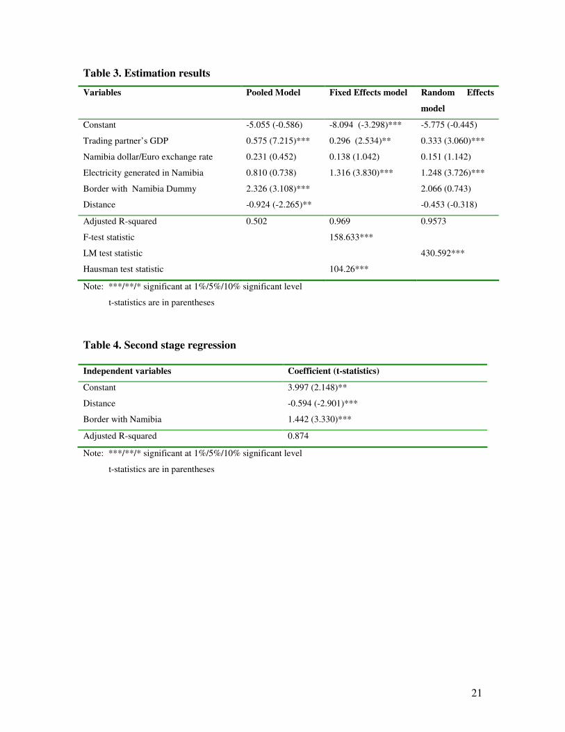
The results for all three models are consistent with the theoretical expectations. The

interpretation of the results focuses on the fixed effects model because it is the

appropriate one. All coefficients are statistically significant, except the Namibia

dollar/Euro exchange rate. The results of the fixed effects model shows that an increase

in trading partner’s GDP income causes tourist arrivals to Namibia to increase. An

increase (depreciation) in the Namibia dollar/Euro exchange rate attract tourist to

Namibia. Increase in electricity generated in Namibia is associated with an increase in

tourist arrivals. This means that it is important to improve infrastructure in order to

increase tourist arrivals. These results compares favourably with other tourism studies in

the literature.

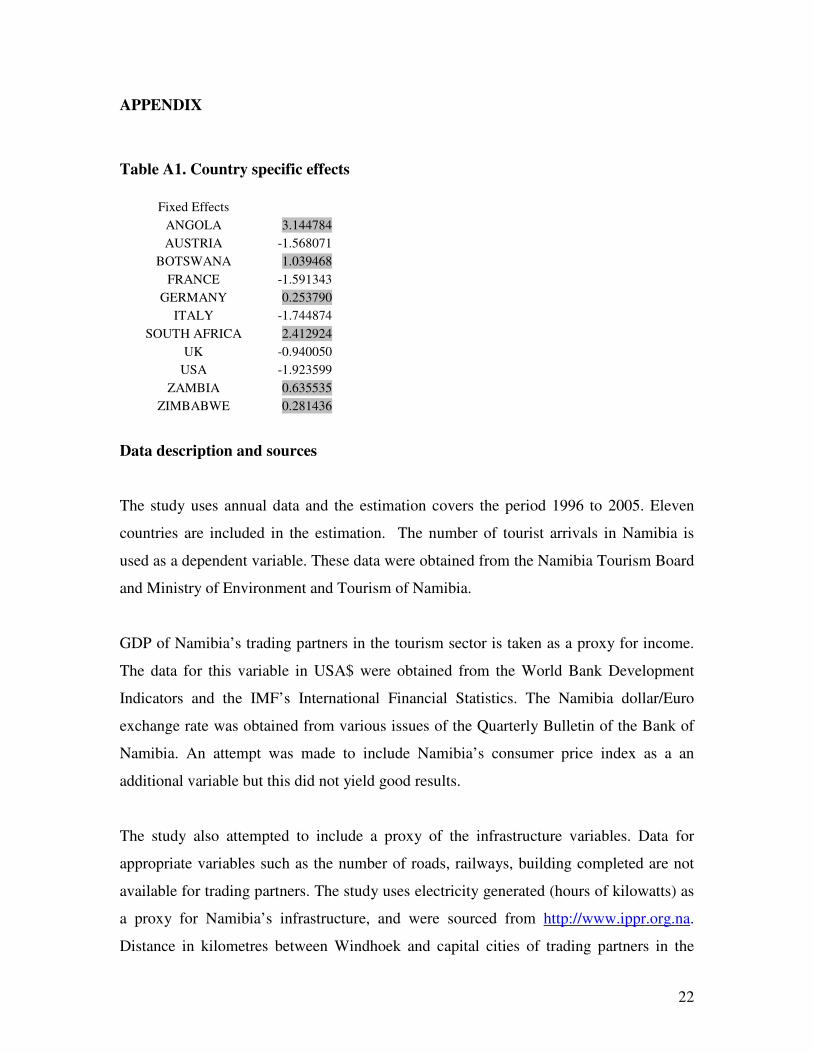
Table A1 in the Appendix presents country specific effects. The country specific effects

show the effects that are unique to each country but not included in the estimation. They

show that tourist arrivals in Namibia differ from country to country and each country is

unique. There are unique features in some countries which promote tourist arrivals in

Namibia from countries such as Botswana, Germany, South Africa, Zambia and

Zimbabwe. These are countries with positive effects and are shaded in Table A1. The

country specific effects also show that there are countries’ characteristics (unobservable)

15

that discourage tourist arrivals in Namibia from countries with negative fixed effects and

not shaded in Table A1. An investigation of the factors which discourage tourist arrivals

in Namibia from countries with negative fixed effects is important for policy making, as

this would help to identify constraints to the tourism sector.

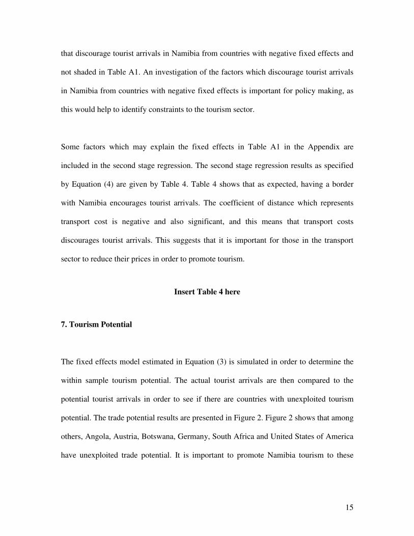
Some factors which may explain the fixed effects in Table A1 in the Appendix are

included in the second stage regression. The second stage regression results as specified

by Equation (4) are given by Table 4. Table 4 shows that as expected, having a border

with Namibia encourages tourist arrivals. The coefficient of distance which represents

transport cost is negative and also significant, and this means that transport costs

discourages tourist arrivals. This suggests that it is important for those in the transport

sector to reduce their prices in order to promote tourism.

Insert Table 4 here

7. Tourism Potential

The fixed effects model estimated in Equation (3) is simulated in order to determine the

within sample tourism potential. The actual tourist arrivals are then compared to the

potential tourist arrivals in order to see if there are countries with unexploited tourism

potential. The trade potential results are presented in Figure 2. Figure 2 shows that among

others, Angola, Austria, Botswana, Germany, South Africa and United States of America

have unexploited trade potential. It is important to promote Namibia tourism to these

16

countries in order to exploit the unexploited tourism potential. A further analysis of each

country to identify possible constraints to Namibia’s tourism is required.

8. Conclusion

This paper investigates the determinants of tourist arrivals in Namibia for the period 1996

to 2005 using a model of international tourism and analysed if there are some markets

with unexploited tourism potential. The study revealed that the main source of tourist

arrivals in Namibia is African countries, mainly neighbouring countries. Neighbouring

countries account for the largest number of tourists followed by Germany, USA and other

European countries.

The model was estimated for 11 main trading partners in the tourism sector. The

estimation results show that trading partners’ income has a positive effect on tourist

arrivals in Namibia. A depreciation of the Namibia dollar/Euro exchange rate and

increase in electricity generated in Namibia attract tourists. Transport costs increase the

cost of travelling and therefore discourage tourist arrivals. Having a border with Namibia

is associated with an increase in tourism arrivals in Namibia. The estimated model was

simulated to determine if there is unexploited tourism potential. The results revealed that

there is unexploited tourism potential in Angola, Austria, Botswana, Germany, South

Africa and United States of America. The results suggest that it is important to promote

tourism to markets where there is unexploited trade potential. Factors which inhibit the

17

tourism sector in Namibia need to be investigated. This can contribute to increase in

economic growth and employment generation.

18

Figure 1. Total number of tourist arrivals in Namibia

0

100000

200000

300000

400000

500000

600000

700000

800000

900000

1996 1997 1998 1999 2000 2001 2002 2003 2004 2005

tourist arrivals

Source: Data obtained from Namibia Tourism Board and Ministry of Environment and Tourism of

Namibia.

Figure 2. Trade Potential (in logs)

Angola Austria

11.4

11.6

11.8

12

12.2

12.4

12.6

12.8

1996 1997 1998 1999 2000 2001 2002 2003 2004 2005

Actual Potential

7.9

8

8.1

8.2

8.3

8.4

8.5

8.6

8.7

8.8

8.9

1996 1997 1998 1999 2000 2001 2002 2003 2004 2005

Actual Potent ial

19

Botswana Germany

9.2

9.4

9.6

9.8

10

10.2

10.4

1996 1997 1998 1999 2000 2001 2002 2003 2004 2005

Actual Potential

10.5

10.6

10.7

10.8

10.9

11

11.1

11.2

11.3

1996 1997 1998 1999 2000 2001 2002 2003 2004 2005

Actual Potential

South Africa United States of America

11.8

11.9

12

12.1

12.2

12.3

12.4

12.5

12.6

1996 1997 1998 1999 2000 2001 2002 2003 2004 2005

Actual Potential

8.7

8.8

8.9

9

9.1

9.2

9.3

9.4

9.5

9.6

1996 1997 1998 1999 2000 2001 2002 2003 2004 2005

Actual Potential

20

Table 1. Top sources of tourist arrivals for Namibia

Market Tourist arrivals

Angola 281365

South Africa 230949

Germany 61222

Zambia 35782

Zimbabwe 22765

Botswana 22333

United Kingdom 20978

United States of America 11979

Netherlands 11569

France 9959

Italy 8557

Switzerland 8363

Scandinavia 6327

Austria 5160

Australia 4274

Total including others 777890

Source: Namibia Tourism Board and Ministry of Environment and Tourism of Namibia

Table 2. Panel Unit root test

Variable IPS test statistic LLC test statistic

GDP of trading partner

Namibia dollar/Euro exchange rate

0.794 (0.786)

2.187 (0.986)

-3.530 (0.000)***

-2.519 (0.006)***

Tourist arrivals -1.713 (0.043)** -3.989 (0.000)***

Electricity generated in Namibia (Namibia’s infrastructure) -1.484 (0.069)* -9.543 (0.000)***

Notes: ***/**/* significant 1%/5%/10% level.

Probabilities are in parentheses.

21

Table 3. Estimation results

Variables Pooled Model Fixed Effects model Random Effects

model

Constant -5.055 (-0.586) -8.094 (-3.298)*** -5.775 (-0.445)

Trading partner’s GDP 0.575 (7.215)*** 0.296 (2.534)** 0.333 (3.060)***

Namibia dollar/Euro exchange rate 0.231 (0.452) 0.138 (1.042) 0.151 (1.142)

Electricity generated in Namibia 0.810 (0.738) 1.316 (3.830)*** 1.248 (3.726)***

Border with Namibia Dummy 2.326 (3.108)*** 2.066 (0.743)

Distance -0.924 (-2.265)** -0.453 (-0.318)

Adjusted R-squared

F-test statistic

LM test statistic

Hausman test statistic

0.502 0.969

158.633***

104.26***

0.9573

430.592***

Note: ***/**/* significant at 1%/5%/10% significant level

t-statistics are in parentheses

Table 4. Second stage regression

Independent variables Coefficient (t-statistics)

Constant 3.997 (2.148)**

Distance -0.594 (-2.901)***

Border with Namibia 1.442 (3.330)***

Adjusted R-squared 0.874

Note: ***/**/* significant at 1%/5%/10% significant level

t-statistics are in parentheses

22

APPENDIX

Table A1. Country specific effects

Fixed Effects

ANGOLA 3.144784

AUSTRIA -1.568071

BOTSWANA 1.039468

FRANCE -1.591343

GERMANY 0.253790

ITALY -1.744874

SOUTH AFRICA 2.412924

UK -0.940050

USA -1.923599

ZAMBIA 0.635535

ZIMBABWE 0.281436

Data description and sources

The study uses annual data and the estimation covers the period 1996 to 2005. Eleven

countries are included in the estimation. The number of tourist arrivals in Namibia is

used as a dependent variable. These data were obtained from the Namibia Tourism Board

and Ministry of Environment and Tourism of Namibia.

GDP of Namibia’s trading partners in the tourism sector is taken as a proxy for income.

The data for this variable in USA$ were obtained from the World Bank Development

Indicators and the IMF’s International Financial Statistics. The Namibia dollar/Euro

exchange rate was obtained from various issues of the Quarterly Bulletin of the Bank of

Namibia. An attempt was made to include Namibia’s consumer price index as a an

additional variable but this did not yield good results.

The study also attempted to include a proxy of the infrastructure variables. Data for

appropriate variables such as the number of roads, railways, building completed are not

available for trading partners. The study uses electricity generated (hours of kilowatts) as

a proxy for Namibia’s infrastructure, and were sourced from http://www.ippr.org.na.

Distance in kilometres between Windhoek and capital cities of trading partners in the

23

tourism sector is used as a proxy for transport costs and were obtained from

http://www.timeanddate.com.

24

9. References

Cheung, C. & Law, R. 2001. Determinants of Tourism Hotel Expenditure in Hong Kong,

International Journal of Contemporary Hospitality Management, 13(3): 151-158.

Divisekera, S. 2003. A Model of Demand for International Tourism, Annals of Tourism

Research, 30(1): 31-49.

Durbarry, R. 2000. Tourism Expenditure in the UK: Analysis of Competitiveness Using a

Gravity-Based Model, Christel DeHaan Tourism and Research Institute Research

Paper 2000/1, Nottingham, Nottingham University Business School.

Egger, P. 2000. A Note on the Proper Econometric Specification of the Gravity

Equation, Economic Letters, 66: 25-31.

Eilat, Y. & Einav, L. 2004. Determinants of International Tourism: A Three-Dimensional

Panel Data Analysis, Applied Economics, 36: 1315-1327.

Hadri, K. (2000) “Testing for Stationarity in Heterogeneous Panel Data”, Econometric

Journal, 3(2): 148-161.

Im, K.S., Pesaran, M.H. and Shin, Y. (2003) “Testing for Unit Roots in Heterogeneous

Panels”, Journal of Econometrics, 115: 53-74.

Katafono, R. & Gounder, A. 2004. Modelling Tourism Demand in Fiji, Reserve Bank of

Fiji Working Paper 2004/01, Suva: Reserve Bank of Fiji.

Lim, C. 1997. Review of International Tourism Demand Models, Annals of Tourism

Research, 24(4): 835-849.

25

Luzzi, G.F. & Flückiger, Y. 2003. An Econometric Estimation of the Demand for

Tourism: The Case of Switzerland, Pacific Economic Review, 8(3): 289-303.

Martinez-Zarzoso, I. and Nowak-Lehmann, F. (2003) “Augmented Gravity Model: An

Empirical Application to Mercosur-European Union Trade Flows”, Journal of

Applied Economics, 6(2): 291-316.

Narayan, P.K. 2005. The Structure of Tourist Expenditure in Fiji: Evidence from Unit

Root Structural Break Tests, Applied Economics, 37: 1157-1161.

Naude, W.A. & Saayman, A. 2004. The Determinants of Tourist Arrivals in Africa: A

Panel Data Regression Analysis, Paper Presented at the International

Conference, Centre for the Study of African Economies, St. Catherine’s College,

University of Oxford, 21-22 March.

Rossello, J., Aguiló, E. & Riera, A. 2005. Modeling Tourism Demand Dynamics, Journal

of Travel Research, 44: 111-116.

Strauss, J. and Yigit, T. 2003. Shortfalls of Panel Unit Root Testing, Economic Letters,

81: 309-313.

Walsh, M. 1997. Demand Analysis in Irish Tourism, Journal of the Statistical and Social

Inquiry Society of Ireland, XXVII (IV): 1-35.

World Travel & Tourism Council. 2006. Namibia: The Impact of Travel & Tourism on

Jobs and the Economy, London: World Travel & Tourism Council.