Embed Size (px)
Citation preview

CONGRESS OF THE UNITED STATESCONGRESSIONAL BUDGET OFFICE
A
CBOS T U D Y
AUGUST 2004
Estimating theValue of
Subsidies forFederal Loans
and LoanGuarantees
© R
oyal
ty-fr
ee/C
orbi
s


CBO
Estimating the Value of Subsidiesfor Federal Loans
and Loan Guarantees
August 2004
A
S T U D Y
The Congress of the United States O Congressional Budget Office


Preface
The Federal Credit Reform Act of 1990 (FCRA) changed the budgetary accounting for federal direct and guaranteed loans from a cash basis to an accrual basis. That shift requires that the government’s expected losses from such loans—because of defaults and interest rate subsidies—be recognized in the budget when the credit is extended. The FCRA specifies that uncertain future cash flows associated with such loans be converted (discounted) to their present values using the interest rates on Treasury securities.
With credit-reform rules having been in effect for more than a decade, the Chairman of the House Budget Committee has asked the Congressional Budget Office (CBO) to reexamine the provisions of the FCRA with an eye toward identifying possible improvements in, and extensions of, that accrual basis of budgetary accounting. This study—which is one part of CBO’s response to that request—focuses on using commercial interest rates, which incorpo-rate risk, instead of risk-free Treasury rates to measure the cost of federal credit programs.
Deborah Lucas, Marvin Phaup, and Ravi Prasad prepared this report under the direction of Roger Hitchner of CBO’s Microeconomic and Financial Studies Division. (Ravi Prasad, now with Bank of America Securities, contributed to this study while serving as a consultant to CBO.) Kim Cawley, Paul Cullinan, Robert Dennis, Peter Fontaine, Kathy Gramp, Arlene Holen, Albert Metz, Elizabeth Robinson, Robert Sunshine, David Torregrosa, Eric Wang, and Thomas Woodward of CBO contributed helpful comments on earlier drafts, and Wendy Kiska provided technical assistance. Susan Woodward of Sand Hill Econometrics and Michael Falkenheim, Robert Kilpatrick, and Sangkyun Park of the Office of Management and Budget reviewed earlier versions of this report; Robert McDonald of Northwestern University offered technical advice. (The assistance of such external participants implies no responsibility for the final product, which rests solely with CBO.)
Christian Spoor edited the study, and John Skeen proofread it. Maureen Costantino produced the cover and prepared the report for publication. Lenny Skutnik printed the initial copies, and Annette Kalicki prepared the electronic versions for CBO’s Web site (www.cbo.gov).
Douglas Holtz-EakinDirector
August 2004

Introduction and Summary 1
Costs Under the FCRA and with Market Prices 3
The Relevance of Market Prices and Market Risk toGovernment Budgeting for Credit Programs 4Is Market Risk Relevant? 4Differences Between the Government
and Private Financial Institutions 5
Methods for Valuing Federal Loans and Guarantees 6The Treasury-Rate Approach 6Risk-Adjusted Discount Rates
and Options-Pricing Methods 7
Estimating the Subsidies to Chrysler andAmerica West Airlines 9Chrysler’s Financial Condition and Guarantee Terms 9AWA’s Financial Condition and Guarantee Terms 10Treasury-Rate Subsidy Estimates 12Market-Value Subsidy Estimates 14
The Effect of Market Risk on Subsidy Rates 15
Uncertainty and Reestimates 15
Appendix A: Volume and Cost of FederalCredit Programs 21
Appendix B: An Example of Using the Binomial Modelto Price a Loan Guarantee 23
Appendix C: Parameter Estimates and ModelingAssumptions Used in This Analysis 25
CONTENTS

vi ESTIMATING THE VALUE OF SUBSIDIES FOR FEDERAL LOANS AND LOAN GUARANTEES
Tables
1. Estimated Federal Costs of Loan Guarantees to Chrysler and America West Airlines 13
2. Estimated Subsidy Rates for Federal Loan Guarantees to Chryslerand America West Airlines 15
3. Initial and Reestimated Federal Costs from the Loan Guaranteeto America West Airlines 17
A-1. Federal Direct and Guaranteed Loans Outstanding, 1994 to 2003 21
A-2. Budget Authority for Subsidies for Federal Direct and Guaranteed Loans, 2003 22
Figures
S-1. Federal Credit Outstanding, 1993 to 2003 2
1. AWA Stock Prices, January 2000 to July 2004 16
2. Probability Distribution of Market Values of the AWA Loan Guarantee 18
3. Probability Distribution of Market Values of the AWA Warrants 19
B-1. Illustrative Possible Values of Assets, Cash Flows, and Bonds in One Year 24
Box
1. Loan Guarantees as Put Options 10

Estimating the Value of Subsidiesfor Federal Loans
and Loan Guarantees
Introduction and SummaryTo achieve some of its policy goals, the federal govern-ment reduces the price and increases the availability of credit for particular uses by guaranteeing private loans or making loans directly. In fiscal year 2003, the govern-ment guaranteed $365 billion in new loans. More than two-thirds of them were for home mortgages, although the government also provides loan guarantees to com-panies in specific sectors, such as the airline, steel, oil, gas, and rural television industries. In addition, the govern-ment extended $36 billion in direct loans in 2003, many of them through its student loan programs. In all, the federal direct and guaranteed loans that were outstanding last year had a total value of $1.4 trillion—nearly two-thirds more than the value 10 years earlier (see Summary Figure 1).1
Those credit activities convey subsidies to borrowers—in the form of more-attractive loan terms than borrowers might otherwise obtain—at a cost to the government. The way that cost is treated in the federal budget has changed over time, most significantly in 1990 with the enactment of the Federal Credit Reform Act (FCRA). That legislation redefined the budgetary cost of federal credit activity: instead of the annual cash flow on all out-standing federal loans and loan guarantees, the budget now records the present value of future cash flows on credit extended in the current budget year. In making that change, the FCRA effectively put the accounting of federal credit on an accrual basis (as is the case for interest on federal debt held by the public and some pension costs for federal employees).2
The government’s estimates of its subsidy costs for loans and loan guarantees are modest, especially in relation to the volume of those loans. For example, the $36 billion in new direct loans obligated in 2003 are estimated to cost the government $657 million over the life of the loans—or $1.83 for each $100 lent (a subsidy rate of 1.83 per-cent).3 Similarly, the $365 billion in new guarantee com-mitments made in 2003 are estimated to cost $4.2 bil-lion—or $1.15 per $100 guaranteed (a subsidy rate of 1.15 percent). Some federal credit programs, such as di-rect student loans and the Federal Housing Administra-tion’s mortgage insurance, appear to make money for the government.
Although the government and private lenders estimate the value of loans and loan guarantees in essentially the same way, two exceptions make government credit pro-grams seem less costly than comparable credit extended by private financial institutions. First, federal agencies’ administrative expenses are not included in estimates of subsidy costs (though they appear elsewhere in the federal budget). Second, those estimates exclude the cost of mar-ket risk—the compensation that investors require for the
1. For more details about the volume and cost of federal credit pro-grams, see Appendix A.
2. See the Federal Credit Reform Act of 1990, included as title XIII, section 13201 of the Omnibus Budget Reconciliation Act of 1990; 2 U.S.C. 661, 104 Stat. 1388-610. See also Congressional Budget Office, Estimating the Costs of One-Sided Bets: How CBO Analyzes Proposals with Asymmetric Uncertainties (October 1999); Office of Management and Budget, “Federal Credit,” part 5 of Preparation, Submission, and Execution of the Budget, Circular No. A-11 (July 2004), available at www.whitehouse.gov/omb/circulars/a11/current_year/s185.pdf; and Marvin Phaup, “Credit Reform, Negative Subsidies, and FHA,” Public Budgeting & Fi-nance, vol. 16, no. 1 (1996), pp. 23-36.
3. Budget of the United States Government, Fiscal Year 2005: Analyti-cal Perspectives, Tables 7-3 and 7-4.

2 ESTIMATING THE VALUE OF SUBSIDIES FOR FEDERAL LOANS AND LOAN GUARANTEES
Summary Figure 1.
Federal Credit Outstanding, 1993 to 2003(Billions of dollars)
Source: Congressional Budget Office based on data from the Office of Management and Budget.
uncertainty of expected but risky cash flows. The reason is that the FCRA requires analysts to calculate present values by discounting expected cash flows at the interest rate on risk-free Treasury securities (the rate at which the government borrows money).4 In contrast, private finan-cial institutions use risk-adjusted discount rates to calcu-late present values.
Despite those limitations, credit-reform accounting pro-vides more-useful cost estimates than did the cash-basis accounting it replaced. The current approach is forward- looking for the life of a loan; it accounts for the time value of money; and it generally assigns the same budget-ary cost to equivalent loans and loan guarantees.
The FCRA adopted the private market’s definition of value (the present value of expected cash flows, with the two exceptions noted above) in an attempt to “place the cost of credit programs on a budgetary basis equivalent to other federal spending . . . and improve the allocation of resources among credit programs and between credit and other spending programs.”5 The costs of other programs in the federal budget are based on market prices—such as the estimated price of buying a weapon, repairing a road, or furnishing a service. In the case of credit programs, however, omitting some of the costs of providing credit results in an overstatement of the value of the govern-ment’s loans and guarantees. One indication of that over-statement is that proposed sales of federal loans to private investors usually appear to result in losses to the govern-ment because the market value of a loan is almost always less than the credit-reform value. The primary reason is the difference in discount rates used by the market and under credit reform.
Following more than a decade of experience with credit reform and rapid advances in financial theory and prac-tice, this Congressional Budget Office (CBO) study re-examines the use of risk-free Treasury rates to value fed-eral loans and guarantees and to estimate their subsidy costs.6 It discusses two approximately equivalent modifi-cations to the current approach, both of which would use market prices: risk-adjusted discounting and options pricing. The analysis then employs options pricing to show how that method’s estimates of federal subsidy costs differ from Treasury-rate estimates for two major govern-ment loan guarantees—those made to Chrysler in 1980 and America West Airlines (AWA) in 2002.
Those two loan guarantees were riskier than the ones typ-ically made under government credit programs. Thus, the difference between market-value estimates of their costs and Treasury-rate estimates would be expected to be greater than for many other programs. Nevertheless, for all programs, ignoring the cost of risk understates the fed-eral cost of credit assistance, potentially biasing the allo-cation of budgetary resources. For example, excluding the
4. Calculations of present value (a single number that expresses a flow of current and future payments in terms of an equivalent lump sum paid today) depend on the particular interest rate used. For example, if $100 is invested on January 1 at an annual interest rate of 5 percent, it will grow to $105 by January 1 of the next year. Hence, under the assumption of a 5 percent annual interest rate (or discount rate), the present value of $105 payable a year from today would be $100.
1993 1995 1997 1999 2001 2003
0
200
400
600
800
1,000
1,200
1,400
1,600
Total
Guaranteed Loans
Direct Loans
5. 2 U.S.C. 661.
6. Although Treasury securities are free from the risk of default, they are subject to other risks, including price risk (the risk that changes in market interest rates or other factors will alter the value of the securities). That risk is reflected in the market prices and yields on Treasury debt. In this study, the term “risk- free Treasury rates” refers only to the default-free quality of those securities.

ESTIMATING THE VALUE OF SUBSIDIES FOR FEDERAL LOANS AND LOAN GUARANTEES 3
cost of risk from budget and program decisions may mis-lead policymakers by suggesting that some federal credit programs provide financial resources to the government at no cost to taxpayers. It also encourages reliance on credit rather than other policies that might be more effi-cient in achieving particular goals.
The principal conclusions of this study are these:
B Market risk is a cost to the government.
B With the exception of administrative costs, projected cash flows on federal loans and loan guarantees are identical under credit-reform and market valuation. The key difference between the two methods is the use of different discount rates.
B Using Treasury rates to discount expected cash flows neglects the cost of market risk and results in the sys-tematic understatement of costs for both direct and guaranteed loans. Using risk-adjusted discount rates, which include the cost of market risk, would correct that understatement and improve the comparability of budgetary costs for credit and other programs.
B For some federal loans and guarantees, risk adjustment can have a significant effect on cost estimates. For in-stance, when the market price of risk is taken into ac-count, the subsidy rate on the Chrysler loan guarantee is 15.9 percent rather than 7.2 percent, CBO esti-mates, and the subsidy rate on the America West guar-antee is 6.9 percent instead of -12.7 percent. For other programs with less exposure to market risk, the effect on subsidy estimates may be much smaller. (Producing estimates for other programs was beyond the scope of this analysis.)
B Which market-pricing method is appropriate to use for a federal credit program depends on the character-istics of the program and of borrowers. This study uses an options-pricing approach to estimate the value of the Chrysler and AWA loan guarantees. That method is well suited to valuing federal loans and guarantees to private companies. For other programs, such as those providing student loans and home mortgage guaran-tees, alternative approaches to adjusting discount rates for risk are likely to be easier to apply.
Costs Under the FCRA and with Market Prices To calculate lifetime costs for new direct and guaranteed loans in a budget year, analysts project the government’s expected cash flows for loan disbursements, defaults, in-terest payments, fees, and repayments for the expected lives of the loans. Those future dollars are converted to present values through discounting to take account of the time value of money (the fact that a dollar tomorrow is worth less than a dollar today because of the interest that could have been earned on that dollar in the meantime). The credit-reform subsidy is the estimated difference be-tween the present value of expected cash outflows and ex-pected cash inflows at the time the credit is extended. As the financial condition of borrowers changes over time, the value of a loan or guarantee also changes. Periodic budget reestimates allow those changes to be recognized in the budget over the life of the loan.
The FCRA mandates that future cash flows be dis-counted using interest rates on marketable Treasury secu-rities with similar maturities to the loans in question. In the case of risk-free loans (those whose cash flows are cer-tain and do not change with the state of the economy), that method results in an estimate of the market value of the loans, just as it does for a promise of payment by the Treasury.7 In the case of risky loans (those whose ex-pected cash flows are uncertain), that procedure systemat-ically overestimates the market value of promised cash flows by discounting at too low a rate. Equivalently, it underestimates the cost of loan guarantees—that is, the value of cash shortfalls that the government has to make up when an underlying loan defaults.
Market prices, by contrast, reflect the fact that risky future cash flows are discounted by investors at risk-adjusted rates. For loans, higher market risk implies a higher discount rate and a lower present value of expected cash flows. Since the value of a loan guarantee is the dif-ference between the value of the loan’s principal and the present value of expected repayments, higher market risk implies a higher value for the guarantee. Private financial institutions use a variety of methods to estimate the mar-
7. In other words, if the Treasury promises with certainty to pay $106 one year from now (backed by the government’s sovereign power to tax and to print money), and the market rate on Trea-sury securities is 6 percent, then the present value of the promise is $100. That result can be confirmed by observing that such a promise will have a current market price of $100.

4 ESTIMATING THE VALUE OF SUBSIDIES FOR FEDERAL LOANS AND LOAN GUARANTEES
ket value of loans and loan guarantees. Some of those ap-proaches could be adapted to valuing federal credit. This study focuses primarily on one widely used method, op-tions pricing, although it also discusses an alternative, risk-adjusted discount rates.
The Relevance of Market Prices and Market Risk to Government Budgeting for Credit ProgramsThe main rationales for using market prices to estimate the cost of federal credit assistance are that such prices provide a comprehensive measure of cost, are consistent with the measurement of other programs’ costs, and offer the best available way to gauge the opportunity costs to society from such credit assistance.8 If the government provides goods or services at a below-market price, it in-curs an opportunity cost on behalf of its stakeholders (taxpayers and beneficiaries of government programs) in the amount of the underpricing. When the government assumes credit risk, that risk is passed on to government stakeholders, and its value represents a cost. With the ex-ception of a few differences described below, the govern-ment is like any financial institution that assumes costly risks on behalf of others. Thus, assumed risks are as rele-vant to the government as to other financial intermediar-ies and constitute a cost to its stakeholders. Relying on market prices offers a straightforward way to measure that cost and one that is consistent with other budgetary prac-tices.9
Market risk arises from the volatility of the economy and from associated changes in the value of aggregate wealth. Because those changes create undesired uncertainty, they are costly to investors and are reflected in market prices. Market risk differs from diversifiable risk, which can effectively be eliminated by pooling it—in the case of
financial assets, for example, by diversifying a portfolio so that unexpected gains on some investments offset unex-pected losses on others. Market risk, by contrast, is associ-ated with economywide increases or decreases in asset val-ues, so it cannot be eliminated through portfolio diversification.10
Is Market Risk Relevant?Some observers have argued that market risk is not a cost to the government and that Treasury rates are appropriate for valuing government cash flows, even if those flows are risky. Two main justifications are sometimes offered for that view: first, that the government can borrow at Trea-sury rates, so its costs are lower than those of other finan-cial institutions; and second, that the government can spread financial risk more widely than other institutions can, effectively making the risk diversifiable and thus without cost to stakeholders.
The first argument—that the government can borrow at a risk-free rate—ignores the role of stakeholders in en-hancing the government’s credit quality. The Treasury can borrow at a relatively low rate (by creating nominally safe securities) in part because of its sovereign power to tax. However, the authority to draw on the resources of others to ensure repayment of debt obligations does not reduce the risk that the government assumes by extending risky loans and guarantees. Rather, it is the means by which such risk is shifted to taxpayers and beneficiaries of government programs, who are, in essence, equity holders in the government’s financial activities.
For example, suppose the government borrows $1,000 through the sale of Treasury securities and makes a risky loan for $1,000. In balance-sheet terms, the government has acquired a risky asset that will pay $1,000 at most and a risk-free liability of $1,000. That transaction adversely affects stakeholders because they now bear more financial risk than before the loan was made: they are liable for re-payment of the government securities, independent of the performance of the loan. If the loan returns only $900, stakeholders lose $100. In fact, financing a loan with a debt issue implies that stakeholders have the equiv-alent of a highly leveraged, and hence very risky, owner-ship position in the loan. The critical implication of that example is that the government’s ability to create a risk-
8. Opportunity cost is the highest value of resources in alternative uses. Putting resources into one activity prevents their use in other activities. The highest value of a forgone alternative is the oppor-tunity cost of the chosen activity.
9. David F. Bradford, “On the Uses of Benefit-Cost Reasoning in Choosing Policy Toward Global Climate Change,” in Paul R. Portney and John P. Weyant, eds., Discounting and Intergenera-tional Equity (Washington, D.C.: Resources for the Future, 1999), pp. 37-43. See also the statement of Douglas Holtz-Eakin, Direc-tor, Congressional Budget Office, “The Economic Costs of Long-Term Federal Obligations,” before the House Committee on the Budget, July 24, 2003.
10. Thomas E. Copeland and J. Fred Weston, Financial Theory and Corporate Policy, 3rd ed. (New York: Addison-Wesley, 1992), Chapter 6.

ESTIMATING THE VALUE OF SUBSIDIES FOR FEDERAL LOANS AND LOAN GUARANTEES 5
free liability results from its sovereign authority to draw on the people’s resources. That authority does not protect stakeholders from market risk, nor does it increase the value of a loan above its market value.
The second argument—that the cost of risk is lower to the government because it can spread the risk more widely—is relevant to diversifiable risk but not to market risk. It is sometimes argued that the government can spread losses more widely over the population than, say, insurance companies can by compelling participation in the risk pool. However, as noted above, market risk can-not be eliminated by diversification because it results from an aggregate change in asset values. Even if the gov-ernment eliminated the diversifiable risk inherent in its lending activities, the associated market risk would re-main. At best, a government guarantee could shift the market risk from one group (lenders) to another (taxpay-ers and other government stakeholders).
A related argument is that the government’s ability to borrow and repay that borrowing with future taxes allows it to reduce market risk by spreading the risk among gen-erations. However, borrowing does not increase total resources; rather, it redistributes existing resources from lenders to borrowers. Moreover, risk is not reduced by the government’s power to print money, because financing credit losses by creating money substitutes an inflation tax for a pecuniary tax. In the end, someone must bear the consequences of unpredictable financial returns, and markets determine a price for assuming that risk.
Differences Between the Government and Private Financial InstitutionsAlthough the government does not have a capacity to bear risk on its own, it may have some advantages over private institutions that reduce its relative borrowing costs. The Treasury benefits from economies of scale in issuing, placing, and servicing debt, which lowers its transaction costs. The high liquidity of Treasury debt also reduces federal borrowing costs. But liquidity does not represent true savings if it comes at a cost to stakeholders through the backstop they provide against losses. In addi-tion, the fact that Treasury securities are exempt from state and local taxes reduces the yield that investors re-quire on them relative to the yield on private borrowing. However, lower state and local tax collections do not rep-resent an economic gain to citizens, who have to pay
more of those taxes to support services because states and localities cannot tax Treasury securities.
More fundamentally, none of those advantages are rele-vant from the perspective that the appropriate measure of the government’s cost of providing credit is its opportu-nity cost. That cost is the least expensive alternative for accomplishing a goal—in other words, the cost of credit provided by private lenders.
The question of the appropriate discount rate for the gov-ernment dates back at least to the classic 1970 paper of Kenneth Arrow and Robert Lind, which formalized the argument that when all risks are diversifiable, the govern-ment’s cost for bearing those risks is minimal.11 Although that paper is widely cited to justify the use of risk-free rates to discount federal cash flows, its conclusions do not apply to situations with market risk. Later authors, such as Robert Merton, distinguish between diversifiable and market risk and include the market price of the latter in their analyses of federal financial programs that have sig-nificant exposure to market risk (such as programs that provide deposit and pension insurance).12
The issue of discount rates also arises in accounting for federal investments in private securities. Without recog-nition of the cost of market risk, the budget will give the appearance that the government can finance itself by bor-rowing at the risk-free rate and investing in a portfolio of risky private securities with an expected return higher than that rate.13
11. Kenneth J. Arrow and Robert C. Lind, “Uncertainty and the Eval-uation of Public Investment Decisions,” American Economic Review, vol. 60, no. 3 (1970), pp. 364-378.
12. Robert C. Merton, “An Analytic Derivation of the Cost of Deposit Insurance and Loan Guarantees: An Application of Mod-ern Option Pricing Theory,” Journal of Banking and Finance, vol. I, no. 1 (June 1977), pp. 3-11; and Merton, “Applications of Option-Pricing Theory: Twenty-Five Years Later,” American Eco-nomic Review, vol. 88, no. 1 (March 1988), pp. 323-349. For a more recent discussion, see Steven Boyce and Richard A. Ippolito, “The Cost of Pension Insurance,” Journal of Risk and Insurance, vol. 69, no. 2 (2002), pp. 121-170.
13. For a parallel discussion of the budgetary treatment of federal investments in equity securities, see Budget of the United States Government, Fiscal Year 2004: Analytical Perspectives, “Railroad Retirement Board Investments,” p. 471; and Congressional Bud-get Office, Evaluating and Accounting for Federal Investment in Corporate Stocks and Other Private Securities (January 2003).

6 ESTIMATING THE VALUE OF SUBSIDIES FOR FEDERAL LOANS AND LOAN GUARANTEES
Methods for Valuing Federal Loans and GuaranteesFor both Treasury-rate and market-value estimates, the subsidy cost is the difference between the value of what the government gives and what it receives in a transac-tion. In the case of a direct loan, the government gives cash now and receives a promise of repayments of princi-pal, interest, and fees in the future. In the case of a loan guarantee, the government commits to pay off the lender if the borrower defaults. For that commitment, the gov-ernment often receives fees paid by the borrower. When the borrower is a publicly traded corporation, the govern-ment sometimes also receives compensation in the form of warrants to purchase stock. (A warrant is a type of call option that gives the government the right to buy shares of the company’s stock in the future for a predetermined price.) To calculate the net cost of such a loan guarantee, it is necessary to value all of the components of the agree-ment: the guarantee itself, the fees, and the warrants. This section explains various methods for determining that value, and the next section applies some of those methods to the guarantees, fees, and warrants in two large federal credit deals.
The Treasury-Rate ApproachUnder current practice, the first step in estimating sub-sidy costs for a direct or guaranteed loan is to project the government’s expected cash inflows and outflows from the transaction. Projected cash flows include the disburse-ment of principal, expected repayments, and fees. Ex-pected values for the government’s cash receipts depend on the probability of default each year, the recovery rate on defaulted loans, the planned repayment (amortiza-tion) schedule of a loan, estimated voluntary prepay-ments, and the fee schedule. As required by the FCRA, projected future cash flows are discounted at Treasury rates to obtain the present value of the direct loan or guarantee.
A few simple examples illustrate the process. First, sup-pose a federal agency makes a direct loan of $100 for one year at the government’s borrowing rate of 5 percent. If the loan is free of credit risk, the agency is certain of being repaid $105 in principal and interest at the end of the year. Under credit reform, the value to the government of that loan at its origination is the discounted present value of $105 in one year. Using the government’s borrowing rate of 5 percent as the discount rate, the loan value (V) is:
1) V = $105/1.05= $100
Because the loan is repaid in full with interest, the present value of the future repayment ($100) is equal to the amount advanced ($100), so the cost of the loan to the government is zero.
Second, suppose the agency makes a loan for the same amount on the same terms but with some credit risk in-volved. On the basis of experience, the agency projects that 25 percent of loans like this one will default at the end of a year. In such defaults, the government expects to recover only $30 from the borrower. Under the current approach, the value of this loan to the government is the present value of the weighted average expected return, with the weights being the probability of default and re-payment in full, respectively.14 That is:
2) V = 0.25 ($30/1.05) + 0.75 ($105/1.05) = 0.25 ($28.57) + 0.75 ($100) = $82.14
In that case, the government has given greater value ($100) than it expects to receive, on average, in return ($82.14). The cost (C) of the direct loan is the difference between value given and received. That is:
3) C = -$100 + [0.25 ($28.57) + 0.75 ($100)] = -$17.86
Third, suppose that instead of making a direct loan, the agency simply guarantees that a private lender making the loan to the same borrower on the same terms will be paid in full if the borrower defaults. As guarantor, the govern-ment will have to pay off the lender 25 percent of the time, in each such case giving the lender $105 in princi-pal and interest and collecting $30 from the borrower. The government’s cost will be the discounted present value of those net payments (given that 75 percent of the time the government will pay nothing). That is:
4) C = 0.25 [(-$105/1.05) + ($30/1.05)] + 0.75 ($0)= 0.25 [-$100 + 28.57] + 0= -$17.86
14. See Congressional Budget Office, Estimating the Costs of One-Sided Bets.

ESTIMATING THE VALUE OF SUBSIDIES FOR FEDERAL LOANS AND LOAN GUARANTEES 7
which is the same as the cost to the government of the di-rect loan in the previous example. That result illustrates the general principle that the cost of a direct loan is the same as the cost of a guarantee made on the same terms with the same risks. In both cases, the budgetary cost is the present value of expected losses.
Although those examples are illustrative, they oversim-plify the analytical difficulty of accurately projecting fu-ture cash flows from federal credit activity. Most federal direct and guaranteed loans have a longer maturity than one year, so defaults and recoveries are spread over a longer period. Moreover, the probability of default and the amount expected to be recovered are likely to vary with many things, including the length of time since origination.
More important, defaults do not occur randomly. They result from economic decisions and factors that can be used to project cash flows more accurately. For example, borrowers rarely default on loans when the value of the asset used as collateral exceeds the amount of the unpaid loan balance. Instead, they can sell the asset, pay off the loan, and keep the difference. To predict defaults and the associated cash flows on some loans, therefore, budget an-alysts could project the expected evolution of the price of the borrower’s assets along with the unpaid balance of the loan. As the price of a collateral asset falls, the probability of default increases. Thus, the probability of default at each point in time can be determined from the probabil-ity distribution of asset prices. And those distributions can be projected into the future on the basis of the start-ing price of the asset, its volatility, and its expected rate of return.
Prepayments—which are permitted without penalty for most federal credit programs—also affect the expected cash flows to the government from direct loans and guar-antees. Prepayments extinguish the risk of default and terminate the collection of fees. Like defaults, prepay-ments are usually economically motivated and can be pre-dicted from rising asset values and other factors associated with attractive refinancing opportunities, such as declin-ing interest rates. Successfully projecting those factors can significantly improve the accuracy of estimates of cash flows to the government.
In practice, time and resource limitations often preclude such detailed modeling of projected cash flows for sub-sidy estimates. Budget analysts have a variety of simpler
methods available for assessing the government’s exposure to the risk of default or prepayment—including, for ex-ample, the use of historical default rates for loans with specific credit ratings. However, focusing on the future evolution of the value of the borrower’s assets is consistent with the rules of credit reform and is a straightforward means of getting at the economic motive for default. It is also the method that most closely parallels modern pri-vate-sector methods for estimating the value of credit guarantees. CBO is currently exploring the usefulness of those methods to budget analysts, both for improving the accuracy of cash flow projections and for providing addi-tional information about the cost of risk.
Risk-Adjusted Discount Rates and Options-Pricing MethodsAs with Treasury-rate estimates, producing market-value estimates of subsidy costs also requires estimating the probability distribution of cash flows over the life of a loan or guarantee. The key difference is that the rates used to discount projected cash flows reflect the market price of risk. The financial sector commonly uses several methods to incorporate the price of market risk into esti-mates of value. For securities that are actively traded, the simplest and most reliable approach is to rely on observed market prices. For loans and guarantees for which market prices are unavailable or unreliable, one alternative is to use an adjusted-discount-rate (ADR) method. Another is to apply options-pricing methods.
Adjusted Discount Rates. The ADR method adds a spread—the difference between the interest rate on a Treasury security and the rate on a risky security—to Treasury rates and uses the resulting adjusted rate to dis-count expected cash flows associated with a loan. That higher rate results in a smaller present value of expected future payments, reflecting the cost of market risk. As be-fore, the subsidy cost of a loan or loan guarantee is the ex-tent to which the present value of expected payments falls short of the loan principal. The procedure is the same for both loans and loan guarantees because, in either case, the loss to the government reflects the shortfall in ex-pected repayment value.
To illustrate, consider the previous example of a $100 one-year loan with a 25 percent chance of default and an expected recovery of $30 in the case of default. If the risk-adjusted discount rate is 7 percent instead of the risk-free rate of 5 percent used in equation 2, the estimated market value of the loan will be:

8 ESTIMATING THE VALUE OF SUBSIDIES FOR FEDERAL LOANS AND LOAN GUARANTEES
5) V = 0.25 ($30/1.07) + 0.75 ($105/1.07) = 0.25 ($28.04) + 0.75 ($98.13) = $80.61
That value is $1.53 less than the estimated value with risk-free discounting; thus, the subsidy cost of the loan is higher by the same amount—$19.39 instead of $17.86. As is always the case, the value of a guarantee on that loan is identical to the subsidy on the loan, because the guar-antor (the government) makes up for the difference be-tween the principal of the loan and the value of what is repaid, which is the $19.39 subsidy cost.
One difficulty in applying the ADR method to a loan or guarantee is that the implicit market risk—and hence the appropriate discount rate—can vary significantly over the life of the loan.15 Another issue is that spreads between Treasury rates and private lending rates are influenced by a variety of factors other than market risk, such as differ-ential tax treatment, transaction costs, and liquidity.16 Some or all of those other factors could be considered legitimate elements of the opportunity cost to the govern-ment of making or guaranteeing loans since they affect people’s willingness to pay for those credit services. If such factors were considered significant, adjustments would be necessary to reflect only that part of the rate spread attributable to market risk.
Options Pricing. The general idea behind options-pricing methods is that assets with the same payoffs must have the same price; otherwise, investors would have the op-portunity to earn a risk-free profit by buying low and sell-ing high. The options-pricing method that CBO used for this analysis—the binomial pricing model—exploits that “no arbitrage” assumption by inferring the value of an option (in this case, a loan guarantee) from the price of a portfolio of assets that has the same payoff to the govern-ment as the guarantee.17 (For an explanation of why a loan guarantee can be considered an option, see Box 1 on page 11.) A highly useful feature of that approach is that
the payoff from a loan guarantee can be approximately replicated using a portfolio made up of risk-free bonds and assets of the borrowing firm, all of whose prices can be estimated.
In principle, both options pricing and risk-adjusted dis-count rates should yield identical subsidy estimates. As a practical matter, they entail different types of approxima-tions. Because options-pricing methods account for the changing risk of loan guarantees over time, they are likely to be more accurate at estimating the market value of subsidies—but only when the necessary data and models are available. Otherwise, they may be difficult or cumber-some to apply.
The practices of private financial institutions offer some guidance about which method is likely to prove the most accurate and feasible in particular cases. Options-pricing methods are often used for estimating the value of credit guarantees to businesses, which suggests that they are most suitable for credit to commercial enterprises. In those cases, the fact that things other than market risk can affect interest rate spreads is less relevant, because the value of the reference assets used for pricing (generally, publicly traded stocks) are less sensitive to those nonrisk factors. Private financial institutions also rely on options-pricing methods to value the option to prepay residential mortgages. Hence, those methods may be applicable to the many government mortgage programs that include a prepayment option. In addition, analysts have used options-pricing methods to value deposit insurance.18
Options-based methods are rarely used, however, to value loans or loan guarantees extended to individuals because of the difficulty of estimating the required variables, such as expected rates of return on borrowers’ assets. For fed-eral loans or guarantees made to individuals (such as stu-dent loans), a more standard approach would be to use
15. For example, many firms use the capital asset pricing model (CAPM) to adjust discount rates for risk when valuing capital investments. For a loan guarantee, the correct CAPM rate and thus the value of the guarantee change with time and with the assets and liabilities of the borrower and so are difficult to esti-mate.
16. See, for example, R. Glenn Hubbard, Money, the Financial System, and the Economy (New York: Addison-Wesley, 1994), pp. 143-155.
17. Appendix B provides an example of how the binomial pricing model might be used to estimate the value of a loan guarantee. For more information about such models, see Robert L. McDonald, Derivatives Markets (New York: Addison-Wesley, 2003), Chapter 10.
18. Alan Marcus and Israel Shaked, “The Valuation of FDIC Deposit Insurance Using Option-Pricing Estimates,” Journal of Money, Credit, and Banking (November 1984), pp. 446-460; and Ehud Ronn and Avinash Verma, “Pricing Risk-Adjusted Deposit Insur-ance: An Option-Based Model,” Journal of Finance (September 1986), pp. 871-895.
ESTIMATING THE VALUE OF SUBSIDIES FOR FEDERAL LOANS AND LOAN GUARANTEES 9
private-sector rates of return on consumer credit of simi-lar quality to identify a risk-adjusted discount rate.19 That rate would be used to discount expected net cash flows and thus to calculate the difference between those flows and the loan principal.
Other federal credit programs—such as loan assistance to sovereign states, municipalities, and special-purpose en-terprises—do not fit directly into either the commercial or consumer categories. Estimating the cost of such pro-grams is difficult even under current budgetary rules be-cause there often is little or no experience with a similar transaction on which to draw. In some of those cases, an options-pricing approach is likely to be feasible; in others, using the ADR method will be preferable.
Estimating the Subsidies to Chrysler and America West AirlinesAs noted in Box 1, options pricing is an especially useful type of risk adjustment for valuing complex loan guaran-tees extended to firms. Accordingly, this analysis illus-trates the effect of risk adjustment on federal credit-subsidy estimates by applying options pricing to the fed-eral guarantees extended to Chrysler and America West Airlines in 1980 and 2002, respectively—two instances of complicated guarantee transactions between the govern-ment and severely distressed companies. For comparison, this analysis also estimates the value of those guarantees using the Treasury-rate approach.
The government’s cost of extending a loan guarantee—whether estimated using Treasury-rate or market-based methods—depends on the present and future financial condition of the borrower and the terms of the guarantee. With both the Chrysler and AWA guarantees, the finan-cial outlook for the firms was highly uncertain and the guarantee terms were complex. That uncertainty and complexity must be addressed regardless of the estimating method used.
Chrysler’s Financial Condition and Guarantee TermsIn the 1970s, rising energy prices and the associated growth in demand for fuel-efficient cars hurt the U.S. auto industry.20 Chrysler was especially hard hit because of its high costs, weak financial condition, and unfavor-able mix of vehicles. By 1979, the company faced a declining market share, a reduced credit rating, and oper-ating losses of more than $1 billion. With its financial survival in doubt, Chrysler asked the federal government for assistance to avoid bankruptcy and possible liquida-tion.
The Congress held hearings on Chrysler’s financial condi-tion in October and November of 1979. Arguments in favor of federal assistance included the temporary nature of Chrysler’s difficulties and their external causes: “a series of energy-related external shocks not of the company’s making, which are unique to the automobile industry.”21 Advocates of assistance also argued that the direct cost of inaction—more than 500,000 job losses and a $3 billion to $10 billion increase in the federal deficit, they claimed—was greater than the maximum cost to the gov-ernment. Opponents of federal assistance argued that the projected social costs of Chrysler’s failure were exaggerated, that federal aid would expose the government to large losses, and that the discipline of the private market would be diminished if the government encouraged expectations that it would intervene to save large failing companies. In the end, lawmakers enacted the Chrysler Corporation Loan Guarantee Act in December 1979.
The following spring, in negotiations between Chrysler and the Secretary of Treasury, the government agreed to a loan guarantee of up to $1.5 billion of principal plus ac-crued interest—contingent on the company’s obtaining $1.5 billion in financial assistance and commitments from nongovernmental sources. The government became Chrysler’s senior creditor, meaning that it would be first in line to take the company’s assets in the event of default. Chrysler also agreed to pay the government an annual guarantee fee of 1.0 percent of the guaranteed amount and to furnish it with warrants for 14.4 million common
19. That rate, which reflects the cost of the capital backing the loans, is generally lower than the quoted borrowing rate, which includes additional compensation for default losses. For an extensive dis-cussion of the cost of capital, see, for example, Richard Brealey and Stewart Myers, Corporate Finance, 7th ed. (New York: McGraw Hill, 2003).
20. This Chrysler analysis is based in part on Robert F. Bruner, Chrysler’s Warrants: September 1983, Case No. UVA-F-0682 (Charlottesville, Va.: University of Virginia, Darden Graduate School of Business Administration, 1991).
21. House Report No. 96-690 to accompany H.R. 5860 and House Conference Report No. 95-730, December 20, 1979.

10 ESTIMATING THE VALUE OF SUBSIDIES FOR FEDERAL LOANS AND LOAN GUARANTEES
shares of Chrysler stock. Those warrants gave the govern-ment the right to buy Chrysler stock at $13 per share through 1990. (Participating banks were also given war-rants on the same terms for nearly 13.3 million shares.)22 With the guarantees, Chrysler was able to borrow at an average interest rate of 12.12 percent, much lower than the 20 percent rate it had paid before receiving the guar-antee.
AWA’s Financial Condition and Guarantee Terms America West Airlines was the eighth largest U.S. passen-ger airline in 2002, with a fleet of 146 planes serving 59 destinations.23 Its operations were concentrated around principal hubs in Phoenix and Las Vegas and a minor hub in Columbus, Ohio. In 2001, AWA flew 20 million passengers and generated $2 billion in revenues.
Box 1.
Loan Guarantees as Put Options
In general, options-pricing methods are applicable to loans and loan guarantees because a loan guarantee is a type of “put option”—a contract that gives the holder the right (though not the obligation) to sell specified assets for a predetermined price, no matter how little they turn out to be worth.1
Suppose a factory owner obtains a put option to sell the factory for a “strike price” of $1 million during the next three months. If the market value of the fac-tory is greater than $1 million, the owner will not ex-ercise the option because other buyers would be likely to pay more than that strike price. However, if the value of the factory falls below $1 million during the life of the option, the owner will exercise the op-tion and gain the difference between the market value of the asset and the strike price. For instance, as illustrated in the figure to the right, if the price of the factory declines to $750,000, the owner will exercise the option to sell at $1 million and make $250,000. In the extreme, if the value of the factory drops to
Payoff to the Holder of an Optionto Sell an Asset for $1 Million
zero, the owner will collect $1 million from the seller (the writer of the option). The put option thereby insures the factory owner against a decline in asset price.
Now consider a buyer who purchases the factory at its current market value of $1 million with money obtained from a federally guaranteed loan secured by the factory. Suppose that with a 100 percent federal guarantee, a bank is willing to lend the buyer $1 mil-lion to purchase the plant. In that case, the potential
1. This discussion draws on “Options Are Insurance,” Chapter 2, Section 5 in Robert L. McDonald, Derivatives Markets (New York: Addison-Wesley, 2003).
0.25
0.75
1.00
1.000
0
Gain (Millions of dollars)
Price of Asset (Millions of dollars)
22. Ultimately, Chrysler borrowed just $1.2 billion and issued less than the full number of warrants. It issued $500 million in notes at 10.35 percent in June 1980, another $300 million in July at 11.40 percent, and $400 million in February 1981 at 14.90 per-cent. The valuations in this analysis are based on the full amount of the initial agreements, since it was not known at the time that less than the full amount would be utilized.
23. America West Holdings Corporation—which trades on the New York Stock Exchange under the symbol AWA—is the parent com-pany of America West Airlines. In 2002, the airline was the only operating subsidiary of America West Holdings, although there is now a second subsidiary (the Leisure Company). This report uses AWA, America West Holdings, and America West Airlines inter-changeably.

ESTIMATING THE VALUE OF SUBSIDIES FOR FEDERAL LOANS AND LOAN GUARANTEES 11
That year was a difficult one for U.S. airlines, however. Earnings were in decline even before the terrorist attacks of September 11 because of a fall in high-yield business traffic, rising fuel costs, and reduced operating margins. The terrorist attacks dramatically worsened the economic condition of the airline industry, including AWA, whose credit rating was downgraded in a series of steps. Moody’s reduced its rating of AWA’s senior unsecured debt from B1 in April 2001 to Ca on November 21, 2001. Standard & Poor’s similarly lowered AWA’s credit rating from B+ on September 18, 2001, to CCC- on November 1, 2001.
In the wake of the September 11 attacks, lawmakers en-acted the Air Transportation Safety and System Stabiliza-tion Act, which allowed airlines to apply for credit guar-antees from the federal government. The credit down-grades described above meant that AWA would have found it expensive—if not impossible—to raise funds in
private markets. Accordingly, in November 2001, the air-line applied for a federal loan guarantee. In January 2002, it received final approval from the Air Transportation Sta-bilization Board for a $380 million guarantee.
Supported by that guarantee, AWA was able to borrow $429 million from private lenders and obtain additional concessions and financing (mainly reductions in rent on aircraft it leased and commitments for future financing). That funding allowed AWA to restructure its debt and lease commitments.24 The AWA loan that the govern-
Box 1.
Continued
payoffs to the borrower from the guarantee would be the same as those shown in the figure for the original owner who held an option to sell the factory. In other words, the guaranteed loan secured by the fac-tory gives the borrower the right to “put” the collat-eral asset to the government at a price equal to the balance on the loan. Of course, the borrower will ex-ercise that option only if the price of the factory falls below the amount of the loan, or $1 million. Thus, the loan guarantee is insurance against a drop in the value of the factory, which was the source of the loan’s credit risk. The loan guarantee shifts the risk of a decline in the price of the collateral asset from the lender to the government.
Thus, the position of a borrower is similar to that of the holder of a put option, whereas the position of the lender or guarantor is akin to that of the writer of the option. That is, the borrower can “sell” (put) the collateral assets to the lender or guarantor at a price equal to the unpaid balance on the loan. In fact, the relationship between the value of collateral assets and of debt is a key factor affecting the likelihood and ex-pected cost of default—just as the value of the un-derlying assets relative to the strike price is key to the value of a put option. When the value of the assets is
substantially above the amount owed, the borrower will refinance or sell the assets and pay off the debt rather than default on the loan obligation. But when the value of the assets is less than the unpaid balance, the borrower no longer has the opportunity to refi-nance or to liquidate the assets and repay the loan obligation. In that case, default is more likely. If de-fault occurs, the guarantor pays the amount due to the lender, seizes the collateral assets, and takes a loss equal to the difference between the promised loan payments and the residual value of the assets. In the case of a loan to a commercial enterprise, the poten-tial range of losses to the guarantor is equivalent to that for a written put option on the assets of the firm with a strike price equal to the face value of the loan.
The correspondence between put options and loan guarantees—along with the availability of computer programs for calculating option values—makes op-tions pricing a natural choice for estimating risk-adjusted subsidy costs for some federal direct and guaranteed loans. Options-pricing methods are espe-cially useful in valuing complex loan guarantees ex-tended to companies, such as the federal guarantees to Chrysler and America West Airlines that are ana-lyzed in this study.
24. As compensation for rent reductions on aircraft and other conces-sions, America West issued some of its lessors approximately $104.5 million in convertible senior notes, with an interest rate of 7.5 percent, which were due in 2009 and guaranteed by the com-pany. AWA also converted its existing revolving credit facility into an $89.9 million term loan maturing in 2007.

12 ESTIMATING THE VALUE OF SUBSIDIES FOR FEDERAL LOANS AND LOAN GUARANTEES
ment guaranteed had a seven-year term with equal repay-ments of principal scheduled for years three to seven. It could also be prepaid at any time without penalty. Be-cause of the guarantee, the loan carried a relatively low in-terest rate—the three-month London interbank offer rate (LIBOR) plus 0.4 percentage points, paid quarterly to the lender.
AWA was also obligated to pay guarantee fees to the gov-ernment and other loan participants equaling 5.5 percent of the loan balance in the first year and 8.0 percent there-after. Those fees left the company with a high effective in-terest rate—LIBOR plus 8.4 percentage points—and thus a strong incentive to prepay the loan if its financial condition improved. As further compensation to the gov-ernment, America West issued it warrants to purchase up to 18.8 million shares of Class B common stock at $3 per share for 10 years.25
Treasury-Rate Subsidy EstimatesThe net cost to the government of the AWA and Chrysler guarantees is the cost of the guarantees minus the value of the warrants and guarantee fees. The value of each of those components is affected by uncertainty about de-fault, prepayment, and future asset and stock values. For this analysis, CBO used the same statistical models to estimate the distribution of future cash flows for both the Treasury-rate and market-value estimates so that only the discount rates would differ between the two sets of esti-mates. To determine the effect of risk adjustment on each component of cost, CBO estimated the value of the guar-antees, warrants, and fees separately.26
Guarantee Value. Under credit reform, the cost of default is the discounted present value of expected federal outlays to lenders resulting from borrowers’ failure to make
scheduled payments, net of any recoveries. Currently, those outlays are discounted to the present using the rate on Treasury securities with the same maturities as the cash flows. The first step in estimating that cost, there-fore, is to specify the annual distribution of the probabil-ity and severity of default.
Various analytical methods are available to model the government’s exposure to the risk that a guaranteed bor-rower will default. A method that takes into account the economic causes of default should be based on the pro-jected path of the value of the borrower’s assets. Such an approach, which CBO used to develop market-value esti-mates as well as Treasury-rate estimates, yields estimates of the probability of default over time and the amounts expected to be recovered in default. In the case of the AWA guarantee, CBO projected the value of the com-pany’s assets on the basis of their value at the time of the guarantee and the historical returns on and volatilities of airline-industry assets as a whole. The distribution of Chrysler’s future asset values was similarly based on his-torical returns and volatilities for the auto industry. (For information about the parameter values used in those cal-culations, see Appendix C.)
Another critical variable in the event of default—the un-paid loan balance—depends in part on the amortization schedule for the guaranteed loan. It is also affected by the probability of voluntary prepayment. The high annual fees paid by AWA suggest that the airline will prepay its loan when it can find more favorable terms from private lenders. In CBO’s analysis, prepayment is assumed to occur when AWA’s asset value rises above the book value of its liabilities. The loan terms that Chrysler received were more favorable, but the automaker was also pro-jected to prepay its loan if the market value of its assets exceeded the value of its liabilities. In those cases, the quality of both AWA’s and Chrysler’s credit would proba-bly rise to the point that they could find private financing at a lower rate than that on their guaranteed loan.
The priority of the government’s claim in the event of de-fault affects the expected recovery from the borrower. In the case of AWA, the government-guaranteed loan has lowest priority in liquidation proceedings—all other debt holders would be paid before the government. In the case of Chrysler, by contrast, the government-guaranteed loan had highest priority after current liabilities.
25. In addition, other loan participants received warrants to purchase as many as 3.8 million shares of AWA’s Class B common stock.
26. The Treasury-rate estimates presented here are not the budget esti-mates that were made at the time of the guarantees. In 2001, CBO estimated the total cost of the Air Transportation Safety and System Stabilization Act (H.R. 2926), which provided authority for the government to guarantee loans to qualified airlines under terms to be agreed to by the Air Transportation Stabilization Board. CBO estimated that under that act, $8 billion in guaran-tees would be issued at an average subsidy rate of 25 percent, for a total cost of $2 billion. (At that point, neither the terms of the guarantees nor the specific recipients were known.) The Chrysler guarantee was issued prior to the Federal Credit Reform Act, so it was accounted for in the budget on a cash basis.

ESTIMATING THE VALUE OF SUBSIDIES FOR FEDERAL LOANS AND LOAN GUARANTEES 13
Table 1.
Estimated Federal Costs of Loan Guarantees to Chryslerand America West Airlines(Millions of dollars)
Source: Congressional Budget Office.
Note: These estimates reflect conditions when the guarantees were made, not the final results.
CBO discounted expected cash flows from the AWA guarantee at a rate of 4 percent (the rate on seven-year Treasury bonds). That procedure yielded a present-value cost of $84.8 million for the AWA guarantee (see Table 1). For Chrysler, expected cash flows were discounted at the then-prevailing 10-year Treasury rate of 10.52 per-cent, producing an estimated cost of $255.5 million. In the Treasury-rate calculations, the value of the Chrysler guarantee is three times that of the AWA guarantee mostly because the guaranteed loan to the automaker was much larger (up to $1.5 billion versus $380 million for AWA).
Warrant Values. As noted above, AWA partially compen-sated the government for the loan guarantee by giving it warrants to buy as many as 18.8 million shares of the company’s Class B common stock at an exercise price of $3 per share (the strike price) for a term of 10 years. Those warrants increase in value with the market price of AWA stock and thus provide the government with addi-tional compensation if its guarantee allows the company to return to profitability. Similarly, Chrysler issued war-
rants to the government to purchase up to 14.4 million shares of Chrysler’s common stock, also with a term of 10 years.
CBO calculated the Treasury-rate value of those warrants with the same type of probabilistic analysis that it used to estimate the cost of the guarantees—in other words, it calculated a probability distribution of future stock prices. The sum of the differences between those proba-bility-weighted prices and the strike price is the expected future value of the warrants. Discounting that future value at a risk-free rate (the same 4 percent and 10.52 percent used above) produces Treasury-rate estimates of the warrants’ value at the time they were issued: $79.7 million in the case of AWA and $119.0 million in the case of Chrysler.
Fees. The present value of the guarantee fees to be paid to the government depends on the same variables that deter-mine the value of the guarantee itself. The probabilities of default and prepayment every year are especially impor-tant because fee income to the government terminates with either event. For each company, CBO used the same assumptions about those variables to value guarantee fees that it used to estimate loan guarantee and warrant val-ues. Besides those probabilities, fee income also depends on the fee rate (a percentage of the outstanding balance) and the amortization schedule of the loan.
AWA agreed to pay guarantee fees of 5.5 percent of the unpaid balance in year one and 8.0 percent in later years as long as the loan was outstanding. Chrysler agreed to pay guarantee fees of 1.0 percent of the unpaid balance each year for the duration of the loan. (In Chrysler’s case, the government-guaranteed loan did not have a planned amortization schedule.) Under the current approach, the present value of expected guarantee fees is $52.5 million for AWA and $28.9 million for Chrysler, CBO estimates.
Net Cost. In Treasury-rate terms, when all of the compo-nents of the loan guarantee are taken into account, the AWA deal is expected to produce a net gain to the govern-ment, in that the value of the warrants and fees that it re-ceived exceeds the value of the loan guarantee by $47.4 million (see Table 1). That gain can be attributed to the assumption under the current approach that the price of market risk is zero. Such an assumption creates the ap-pearance that AWA paid the government more than the value of its guarantee. If that were true, then AWA should have rejected the offered terms because it should have
America West Chrysler
Treasury-Rate Estimates
Loan Guarantee -84.8 -255.5Warrants 79.7 119.0Guarantee Fees 52.5 28.9
Net Gain or Loss (-) to the Government 47.4 -107.6
Market-Value Estimates
Loan Guarantee -133.2 -347.5Warrants 50.4 80.6Guarantee Fees 56.6 27.9
Net Gain or Loss (-) to the Government -26.3 -239.0
14 ESTIMATING THE VALUE OF SUBSIDIES FOR FEDERAL LOANS AND LOAN GUARANTEES
been able to obtain credit support on more-favorable terms privately.
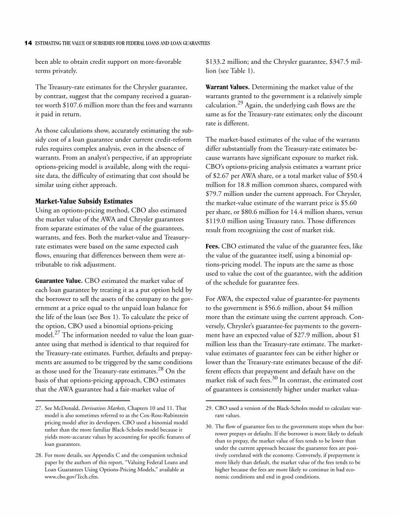
The Treasury-rate estimates for the Chrysler guarantee, by contrast, suggest that the company received a guaran-tee worth $107.6 million more than the fees and warrants it paid in return.
As those calculations show, accurately estimating the sub-sidy cost of a loan guarantee under current credit-reform rules requires complex analysis, even in the absence of warrants. From an analyst’s perspective, if an appropriate options-pricing model is available, along with the requi-site data, the difficulty of estimating that cost should be similar using either approach.
Market-Value Subsidy EstimatesUsing an options-pricing method, CBO also estimated the market value of the AWA and Chrysler guarantees from separate estimates of the value of the guarantees, warrants, and fees. Both the market-value and Treasury-rate estimates were based on the same expected cash flows, ensuring that differences between them were at-tributable to risk adjustment.
Guarantee Value. CBO estimated the market value of each loan guarantee by treating it as a put option held by the borrower to sell the assets of the company to the gov-ernment at a price equal to the unpaid loan balance for the life of the loan (see Box 1). To calculate the price of the option, CBO used a binomial options-pricing model.27 The information needed to value the loan guar-antee using that method is identical to that required for the Treasury-rate estimates. Further, defaults and prepay-ments are assumed to be triggered by the same conditions as those used for the Treasury-rate estimates.28 On the basis of that options-pricing approach, CBO estimates that the AWA guarantee had a fair-market value of
$133.2 million; and the Chrysler guarantee, $347.5 mil-lion (see Table 1).
Warrant Values. Determining the market value of the warrants granted to the government is a relatively simple calculation.29 Again, the underlying cash flows are the same as for the Treasury-rate estimates; only the discount rate is different.
The market-based estimates of the value of the warrants differ substantially from the Treasury-rate estimates be-cause warrants have significant exposure to market risk. CBO’s options-pricing analysis estimates a warrant price of $2.67 per AWA share, or a total market value of $50.4 million for 18.8 million common shares, compared with $79.7 million under the current approach. For Chrysler, the market-value estimate of the warrant price is $5.60 per share, or $80.6 million for 14.4 million shares, versus $119.0 million using Treasury rates. Those differences result from recognizing the cost of market risk.
Fees. CBO estimated the value of the guarantee fees, like the value of the guarantee itself, using a binomial op-tions-pricing model. The inputs are the same as those used to value the cost of the guarantee, with the addition of the schedule for guarantee fees.
For AWA, the expected value of guarantee-fee payments to the government is $56.6 million, about $4 million more than the estimate using the current approach. Con-versely, Chrysler’s guarantee-fee payments to the govern-ment have an expected value of $27.9 million, about $1 million less than the Treasury-rate estimate. The market-value estimates of guarantee fees can be either higher or lower than the Treasury-rate estimates because of the dif-ferent effects that prepayment and default have on the market risk of such fees.30 In contrast, the estimated cost of guarantees is consistently higher under market valua-
27. See McDonald, Derivatives Markets, Chapters 10 and 11. That model is also sometimes referred to as the Cox-Ross-Rubinstein pricing model after its developers. CBO used a binomial model rather than the more familiar Black-Scholes model because it yields more-accurate values by accounting for specific features of loan guarantees.
28. For more details, see Appendix C and the companion technical paper by the authors of this report, “Valuing Federal Loans and Loan Guarantees Using Options-Pricing Models,” available at www.cbo.gov/Tech.cfm.
29. CBO used a version of the Black-Scholes model to calculate war-rant values.
30. The flow of guarantee fees to the government stops when the bor-rower prepays or defaults. If the borrower is more likely to default than to prepay, the market value of fees tends to be lower than under the current approach because the guarantee fees are posi-tively correlated with the economy. Conversely, if prepayment is more likely than default, the market value of the fees tends to be higher because the fees are more likely to continue in bad eco-nomic conditions and end in good conditions.
ESTIMATING THE VALUE OF SUBSIDIES FOR FEDERAL LOANS AND LOAN GUARANTEES 15
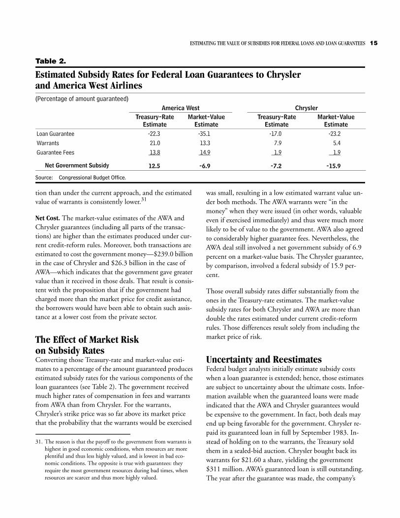
Table 2.
Estimated Subsidy Rates for Federal Loan Guarantees to Chryslerand America West Airlines(Percentage of amount guaranteed)
Source: Congressional Budget Office.
tion than under the current approach, and the estimated value of warrants is consistently lower.31
Net Cost. The market-value estimates of the AWA and Chrysler guarantees (including all parts of the transac-tions) are higher than the estimates produced under cur-rent credit-reform rules. Moreover, both transactions are estimated to cost the government money—$239.0 billion in the case of Chrysler and $26.3 billion in the case of AWA—which indicates that the government gave greater value than it received in those deals. That result is consis-tent with the proposition that if the government had charged more than the market price for credit assistance, the borrowers would have been able to obtain such assis-tance at a lower cost from the private sector.
The Effect of Market Risk on Subsidy RatesConverting those Treasury-rate and market-value esti-mates to a percentage of the amount guaranteed produces estimated subsidy rates for the various components of the loan guarantees (see Table 2). The government received much higher rates of compensation in fees and warrants from AWA than from Chrysler. For the warrants, Chrysler’s strike price was so far above its market price that the probability that the warrants would be exercised
was small, resulting in a low estimated warrant value un-der both methods. The AWA warrants were “in the money” when they were issued (in other words, valuable even if exercised immediately) and thus were much more likely to be of value to the government. AWA also agreed to considerably higher guarantee fees. Nevertheless, the AWA deal still involved a net government subsidy of 6.9 percent on a market-value basis. The Chrysler guarantee, by comparison, involved a federal subsidy of 15.9 per-cent.
Those overall subsidy rates differ substantially from the ones in the Treasury-rate estimates. The market-value subsidy rates for both Chrysler and AWA are more than double the rates estimated under current credit-reform rules. Those differences result solely from including the market price of risk.
Uncertainty and ReestimatesFederal budget analysts initially estimate subsidy costs when a loan guarantee is extended; hence, those estimates are subject to uncertainty about the ultimate costs. Infor-mation available when the guaranteed loans were made indicated that the AWA and Chrysler guarantees would be expensive to the government. In fact, both deals may end up being favorable for the government. Chrysler re-paid its guaranteed loan in full by September 1983. In-stead of holding on to the warrants, the Treasury sold them in a sealed-bid auction. Chrysler bought back its warrants for $21.60 a share, yielding the government $311 million. AWA’s guaranteed loan is still outstanding. The year after the guarantee was made, the company’s
America West ChryslerTreasury-Rate
EstimateMarket-Value
EstimateTreasury-Rate
EstimateMarket-Value
EstimateLoan Guarantee -22.3 -35.1 -17.0 -23.2Warrants 21.0 13.3 7.9 5.4Guarantee Fees 13.8 14.9 1.9 1.9
Net Government Subsidy 12.5 -6.9 -7.2 -15.9
31. The reason is that the payoff to the government from warrants is highest in good economic conditions, when resources are more plentiful and thus less highly valued, and is lowest in bad eco-nomic conditions. The opposite is true with guarantees: they require the most government resources during bad times, when resources are scarcer and thus more highly valued.

16 ESTIMATING THE VALUE OF SUBSIDIES FOR FEDERAL LOANS AND LOAN GUARANTEES
Figure 1.
AWA Stock Prices, January 2000 to July 2004(Dollars)
Source: Standard & Poor’s COMPUSTAT database.
stock price declined, but it rebounded thereafter (see Fig-ure 1). In March 2004, the price stood at more than $9 per share, implying that if the government exercised its $3 per-share warrants at that price, it would gain more than $100 million. (Since then, AWA’s stock price has de-clined further, but at $6 per share, it remains above the warrant price.)
Those cases might suggest that Treasury-rate subsidy esti-mates are too high rather than too low. However, a more valid conclusion is that such estimates are uncertain. In fact, many examples exist of loan guarantees whose value has deteriorated over time. For instance, the $100 billion in loan guarantees that the Federal Housing Administra-tion’s Mutual Mortgage Insurance Fund made in 2000 were initially estimated to net the government approxi-mately $2 billion. Since then, that estimate has been revised three times to indicate progressively smaller ex-pected gains. Currently, those loan guarantees are pro-jected to net only about $680 million—one-third of the amount originally estimated.32
The Federal Credit Reform Act recognizes that subsidy costs are uncertain and that realized gains and losses will deviate from initial estimates. It deals with that uncer-tainty in a logical way: by allowing analysts to make the best estimate possible when a loan or guarantee is origi-nated and then revise that estimate as new information becomes available. Under the FCRA, initial subsidy esti-mates are reestimated over the life of a loan or guarantee to reflect actual cash flows and other factors.33 The origi-nal estimate plus the sum of lifetime reestimates equals the realized subsidy. Consistent with the principles of ac-crual accounting, those reestimates are included in annual budget outlays and in the budget deficit or surplus.34
Market-value reestimates can be calculated analogously to Treasury-rate reestimates, using the same models initially
Jan-00 Ju l-00 Jan-01 Ju l-01 Jan-02 Ju l-02 Jan-03 Ju l-03 Jan-04 Ju l-040
2
4
6
8
10
12
14
16
18
20
A W A R ece ives
Federa l Loan
G uarantee
32. See the Office of Management and Budget’s annual Federal Credit Supplement for fiscal years 2003, 2004, and 2005, Table 8.
33. The Office of Management and Budget currently requires two types of reestimates. The first type is a one-time adjustment for interest rates, which corrects for any discrepancy between interest rates at the time of the original estimate and interest rates at the time the loans are disbursed. The second type is an annual techni-cal reestimate, which adjusts for factors such as changes in prepay-ments, defaults, and recoveries (but not interest rates).
34. See Congressional Budget Office, Credit Subsidy Reestimates, 1993-1999 (September 2000).

Table 3.
Initial and Reestimated Federal Costs from the Loan Guaranteeto America West Airlines(Millions of dollars)
Source: Congressional Budget Office.
Note: Reestimates are recorded in the federal budget as the change in subsidy value since the previous estimate or reestimate. For clarity, this table shows the subsidy value, not its change.
used to calculate subsidy values.35 Reestimation involves updating the parameters of a model to reflect differences between initial assumptions and current information. For comparative purposes, CBO calculated both types of re-estimates for the AWA loan guarantee.36 In that case, the key variable driving the reestimates is stock price. The drop in the company’s stock price during the first year that the loan was outstanding implies a significant in-crease in the probability and severity of future default and thus a sharp decline in the value of the warrants. Both of those factors increase the estimated subsidy cost of the guarantee after one year—from a government gain of $47.4 million to a loss of $115.5 million under current credit-reform rules or from a loss of $26.3 million to a loss of $180.9 million with market risk taken into ac-count (see Table 3). By January 2004, however, AWA’s greatly improved financial condition changed the net subsidy cost into an expected gain: of $250.0 million in
the Treasury-rate estimates or $229.6 million in the mar-ket-value estimates.
The probabilistic models that underlie both the Treasury-rate and market-value estimates are useful for depicting the probability distribution of future guarantee costs and thus the uncertainty associated with the initial cost esti-mates. The probability distribution of the future market value of the AWA guarantee, projected forward two years from January 2002 (when the guarantee was approved), is shown in Figure 2. That guarantee value has a lower bound of zero, which reflects the possibility of a large in-crease in asset value that enables AWA to prepay the loan, extinguishing the value of the guarantee. It has an upper bound of $380 million, the figure that results when AWA’s asset value falls to the point where default occurs and the government recovers nothing from the company. The distribution in Figure 2 suggests that the most prob-able event, looking ahead two years, is a market value between $50 million and $100 million for the AWA guarantee. In that case, the company would still be oper-ating, but the guarantee would remain costly to the gov-
OriginalEstimate
January 2003Reestimate
January 2004Reestimate
Loan Guarantee
Market-Value Estimate -133.2 -241.8 -8.2Treasury-Rate Estimate -84.8 -189.9 -3.9
Warrants
Market-Value Estimate 50.4 13.7 231.6Treasury-Rate Estimate 79.7 24.2 249.1
Guarantee Fees
Market-Value Estimate 56.6 47.2 6.1Treasury-Rate Estimate 52.5 50.2 4.8
Net Gain or Loss (-) to the Government
Market-Value Estimate -26.3 -180.9 229.6Treasury-Rate Estimate 47.4 -115.5 250.0
35. To account for the price of risk more accurately, the reestimate could be adjusted with a charge for market risk.
36. CBO did not produce reestimates for the Chrysler guarantee because the requisite historical data were not readily available.

18 ESTIMATING THE VALUE OF SUBSIDIES FOR FEDERAL LOANS AND LOAN GUARANTEES
Figure 2.
Probability Distribution of Market Values of the AWA Loan GuaranteeProbability (Percent)
Source: Congressional Budget Office.
Note: These numbers are two-year projections looking forward from January 2002, when the America West Airlines (AWA) loan guarantee was approved.
ernment because of the significant possibility of a default during the five years left on the loan.
The projected market-value distributions of fee income and warrant values can be obtained similarly by project-ing the distributions of future cash flows from fees and warrants. (The distribution for warrant values is shown in Figure 3.) Indeed, much of the variation in CBO’s reesti-mates for AWA can be attributed to the high volatility of future warrant values, which is a consequence of the com-pany’s highly volatile stock price.
The distributions of future guarantee and warrant values shown in Figures 2 and 3 reveal that the January 2004 re-estimates for AWA were extremely unlikely from the per-spective of January 2002. The vertical line in Figure 2 in-dicates the guarantee value corresponding to AWA’s asset value at the end of 2003. As the figure illustrates, the probability of such a large reduction in guarantee value was small. Similarly, the vertical line in Figure 3 indicates that it was extremely unlikely that the value of the war-rants would rise to the level that occurred.
FFFFF
F
F
F
F
F
F
F
F
F
F
F
F F F F
F
F
F
F
F
F
F
F
F
F
F
FFFFF0
1
2
3
4
5
6
7
0 50 100 150 200 250 300 350 400
January 2004Reestimate:$8.2 million
Market Value of Guarantee(Millions of dollars)

ESTIMATING THE VALUE OF SUBSIDIES FOR FEDERAL LOANS AND LOAN GUARANTEES 19
Figure 3.
Probability Distribution of Market Values of the AWA WarrantsProbability (Percent)
Source: Congressional Budget Office.
Note: These numbers are two-year projections looking forward from January 2002, when the America West Airlines (AWA) loan guarantee was approved.
FF
F
F
F
F
F
F
F
F
F
F
F
FFFF
F
F
F
F
F
F
F
F
F
F
F
FFFFF0
1
2
3
4
5
6
7
0 50 100 150 200 250 300 350 400 450 500
January 2004Reestimate:$231.6 million
Market Value of Warrants(Millions of dollars)


AVolume and Cost of Federal
Credit Programs
The tables in this appendix offer a sense of the scale of the federal government’s credit programs by detailing the total amounts of direct loans and loan guarantees that were outstanding at the end of each of the past 10 fiscal
years (see Table A-1). They also show the budget author-ity provided for the subsidy costs of those loans and guar-antees in 2003 (see Table A-2). In both cases, the num-bers are broken down by major credit programs.
Table A-1.
Federal Direct and Guaranteed Loans Outstanding, 1994 to 2003(Billions of dollars)
Source: Congressional Budget Office based on data from the Office of Management and Budget.
Notes: * = less than $50 million; FHA = Federal Housing Administration; VA = Department of Veterans Affairs; FFEL = Federal Family Edu-cation Loan program.
Excludes defaults on guarantees that result in recoveries. Excludes secondary loan guarantees issued by the Government National Mortgage Association.
APP ENDIX
1994 1995 1996 1997 1998 1999 2000 2001 2002 2003
Direct Loans
Ford Student Loans * 2.8 11.6 21.2 31.7 45.8 57.7 70.5 80.1 84.5Rural Housing and Community Development 35.3 36.2 36.3 36.4 36.3 35.2 33.3 33.5 33.4 32.9Rural Electrification, Telephone, and Telecommunications 37.6 37.4 35.5 34.0 33.6 33.1 32.1 31.2 31.7 32.1Export-Import Bank 7.5 7.6 7.9 10.1 10.8 12.2 11.1 11.7 11.4 11.1Other 78.8 79.3 75.2 79.7 73.4 74.1 73.9 66.4 63.4 58.7
Total 159.2 163.3 166.5 181.4 185.8 200.4 208.1 213.3 220.0 219.3
Loan Guarantees
FHA Housing 381.9 401.4 455.2 448.6 469.6 504.1 548.5 557.9 563.4 496.4VA Housing 155.0 154.5 154.8 170.5 200.2 221.3 224.3 236.9 264.5 323.1FFEL Student Loans 75.0 86.1 101.9 101.0 100.5 126.7 144.2 159.3 181.9 213.3Small Business Administration 23.6 28.6 30.9 35.2 37.5 39.4 33.8 36.6 41.1 53.4Export-Import Bank 16.8 17.8 17.8 22.1 21.8 25.4 29.8 30.5 31.0 33.5Other 46.5 38.4 45.5 44.5 52.1 58.9 62.3 62.9 63.7 64.8
Total 698.8 726.8 806.1 821.9 881.7 975.8 1,042.9 1,084.1 1,145.6 1,184.4
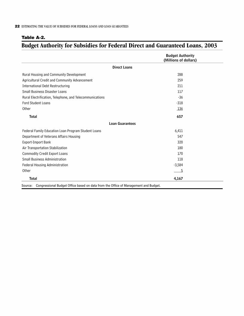
22 ESTIMATING THE VALUE OF SUBSIDIES FOR FEDERAL LOANS AND LOAN GUARANTEES
Table A-2.
Budget Authority for Subsidies for Federal Direct and Guaranteed Loans, 2003
Source: Congressional Budget Office based on data from the Office of Management and Budget.
Budget Authority(Millions of dollars)
Direct Loans
Rural Housing and Community Development 288Agricultural Credit and Community Advancement 259International Debt Restructuring 211Small Business Disaster Loans 117Rural Electrification, Telephone, and Telecommunications -36Ford Student Loans -318Other 136
Total 657
Loan Guarantees
Federal Family Education Loan Program Student Loans 6,411Department of Veterans Affairs Housing 547Export-Import Bank 320Air Transportation Stabilization 180Commodity Credit Export Loans 170Small Business Administration 118Federal Housing Administration -3,584Other 5
Total 4,167

BAn Example of Using the Binomial Model
to Price a Loan Guarantee
A ssume that the federal government guarantees the repayment of principal and interest on $90 million in debt coming due in one year issued by a company with assets of $100 million. The guarantor has effectively given the owner of the company the equivalent of a “put option” on the company’s assets with a “strike price” of $90. That is, the guarantee gives the borrower (the com-pany) the right to sell its assets to the guarantor for $90, whatever their current market value. Suppose that in one year, those assets will be worth either $140 million or $70 million (as shown in the top tree diagram in Figure B-1). If the asset value rises to $140 million, the firm will be able to repay its $90 million debt without any contribu-tion from the federal government. If the asset value falls to $70 million, however, the company will be unable to meet its debt obligation. In that case, it will “put” its as-sets to the government, which will pay $90 million to the lender and sell the assets for $70 million.
Thus, the tree of the borrower’s asset values in Figure B-1 implies the tree of cash flows for the government guaran-tor shown in the middle diagram of the figure. If the company’s asset value increases, the guarantee requires no payment by the government (the put option will expire unexercised); but if the asset value falls, the government will face net costs of $20 million ($90 million minus $70 million) to honor its guarantee.
The cost to the government of that guarantee when it is issued is the present value (P) of the distribution of possi-ble cash flows in one year. That value can be inferred from the price of a portfolio composed of assets of the borrowing firm and risk-free bonds that has the same payoff to the government as the guarantee. If the payoffs are the same, the cost must be the same, and the cost of
the guarantee can be inferred from the known prices of the borrower’s assets and risk-free bonds.
Suppose a risk-free zero-coupon bond with a face value of $100 and a maturity of one year has a current price of $95. Because the bond is risk-free, its value will be $100 in one year regardless of what happens to the value of the firm’s assets (see the bottom tree diagram in Figure B-1). The problem of the value of the loan guarantee is thus re-duced to the following question: how many risk-free bonds (X) and units of the borrower’s assets (Y) are re-quired to generate the same payoff as the guarantee? The payoffs for both the guarantee and the portfolio need to match in both good and bad states of the economy. Thus:
X100 + Y140 = 0 (good states)X100 + Y70 = -20 (bad states)
Those two equations can be solved for X and Y: X = -0.4 and Y = 0.2857. The price of the portfolio—based on the $95 price of the bond and the $100 current asset value—is -0.4($95) + 0.2857($100) = -$9.43. Thus, the guaran-tee is equivalent to selling -0.4 of the risk-free bonds (borrowing 0.4 x $95) at the risk-free rate and buying 0.2857 of the assets. And the cost of the guarantee is the value of the portfolio, or -$9.43.
The value of that guarantee, or option, was inferred with-out an explicit assumption or information about the probabilities of the two possible outcomes. In valuing the federal loan guarantees to Chrysler and America West Airlines, however, the probabilities of up and down moves and the asset value of an up move were estimated using a required rate of return on company assets and the volatility of that return.
APP ENDIX

24 ESTIMATING THE VALUE OF SUBSIDIES FOR FEDERAL LOANS AND LOAN GUARANTEES
To illustrate the relationship among those variables, as-sume that the probability of an up move is 0.6 and that of a down move is 0.4. Those probabilities are consistent
Figure B-1.
Illustrative Possible Values of Assets,Cash Flows, and Bonds in One Year
Source: Congressional Budget Office.
with an expected rate of return on assets of 12 percent (because [0.4(70) + 0.6(140)]/1.12 = 100). The risk-free interest rate can also be inferred from the equation 100/(1 + r) = 95, which implies a rate of 5.26 percent.
The government as guarantor has a portfolio position equivalent to a highly leveraged position in the firm’s as-sets—that is, issuing debt of $38 (0.4 x $95) and buying $28.57 of the firm’s assets. The market value of that port-folio is -$9.43, which is the fee the guarantor must be paid to accept the chance of losing $20. Using the proba-bilities inferred from market returns, the expected loss is 0.4($20) = $8.
Viewed from the lender’s perspective, the lender values an expected payment of $8 in one year at $9.43 today. The discount rate implied by 8/(1 + r) = 9.43 is -15.16 percent, or about 20 percentage points lower than the risk-free rate of 5.26 percent. The expected loss of $8 dis-counted at 5.26 percent has a present value of $7.60, which understates the value of the guarantee by about 19 percent.
That example illustrates that although future cash out-flows on loan guarantees are risky, their risk-adjusted dis-count rate (unlike that of future cash inflows on loans) is not higher than the risk-free rate. The market implicitly discounts expected guarantee payments at an interest rate below the risk-free rate. The reason is that a loan guaran-tee transfers market risk from the lender to the guarantor. For the guarantor to get a commensurate return for as-suming the market risk, the expected payments must be discounted at a rate lower than the risk-free rate. The borrower is paying the risk-free rate to the lender plus compensation to the guarantor for taking on the market risk, which has the effect of making the market value of the guarantee higher than the value obtained from dis-counting at the risk-free rate or an upwardly adjusted rate. Indeed, the guarantee has more market risk than the underlying assets because the guarantee is equivalent to a leveraged position in the assets, which always has more risk than the assets themselves do.
Possible Values of Borrower's Assets in One Year
Possible Values of Government's Cash Flowsfrom Guarantee in One Year
Possible Values of GovernmentZero-Coupon Bond in One Year

CParameter Estimates and Modeling Assumptions
Used in This Analysis
This appendix provides additional information about some of the key parameters and behavioral rules that the Congressional Budget Office (CBO) used to esti-mate the value—under both current credit-reform rules and market valuation—of federal loan guarantees to Chrysler and America West Airlines (AWA). A compan-ion technical paper by the authors of this report, titled “Valuing Federal Loans and Loan Guarantees Using Op-tions-Pricing Methods,” contains details about the under-lying options-pricing models.1
Asset VolatilityA critical input into both Treasury-rate and options-based estimates is the volatility of a firm’s asset value. Although that volatility is not directly observable, it can be esti-mated in a variety of ways. For AWA, this study uses a formula implied by the Black-Scholes options-pricing model:
C1) Volatility of Assets = Volatility of Equity (beta of As-sets/beta of Equity)
The “beta” of a stock or asset is a measure of the correla-tion of its returns with those of the overall market. For publicly traded companies, estimates of equity betas are available from various public sources. Estimates of asset betas are also available for many industries.
The equity beta of AWA’s stock is 1.55.2 The beta of AWA’s assets was set to equal the unlevered beta of the air-line industry (to remove the effect of debt), which is esti-mated at 0.67.3 The equity-volatility range that AWA
uses to value its employee stock options is 44.9 percent to 60 percent. On the basis of those parameters, CBO esti-mated the asset volatility at 19.4 percent to 25.9 percent. The estimates reported in this study use the high end of that range since it accords with independent estimates of asset volatility for the airline industry.
CBO used a different method to estimate asset volatility for Chrysler because not all of the necessary inputs for equation C1 were readily available. That company’s asset volatility was set to equal an average asset volatility for several firms in the automotive industry.4 The current average volatility for automotive firms is 22.5 percent. Although the equity volatility of a particular company can change substantially in a short time, the asset volatil-ity of an industry is likely to be more stable. Nonetheless, the 22 years between 1980 and 2002 are long enough for asset volatility to have altered greatly, and a more careful measure of that variable is recommended for any actual cost estimate.
Market Value of AssetsFor healthy publicly traded firms, adding the market value of equity to the book value of debt liabilities ap-proximates the market value of assets. For financially dis-tressed companies, the book value of debt is likely to be much higher than its market value, but obtaining accu-rate estimates of that market value is difficult. As ex-plained in the companion technical paper, an options-pricing formula can be used interactively to estimate the
APP ENDIX
1. That paper is available at www.cbo.gov/Tech.cfm.
2. Market data for AWA from Bloomberg (www.bloomberg.com).
3. “Damodaran Online,” Web site of Prof. Aswath Damodaran, Stern School of Business, New York University (www.stern.nyu. edu/~adamodar).
4. Ibid.

26 ESTIMATING THE VALUE OF SUBSIDIES FOR FEDERAL LOANS AND LOAN GUARANTEES
market value of assets without requiring an estimate of the market value of debt. That is the approach that CBO took for this analysis.
Using options-pricing formulas to estimate the market price of assets requires the following six measures:
B Market value of equity,
B Volatility of returns on assets,
B Volatility of returns on equity,
B Risk-free interest rate,
B Strike price of the option, and
B Maturity of the debt.
For AWA, the initial market value of equity is $138 mil-lion (based on a share price of $4 and 34.6 million out-standing shares). The volatility of assets is 25.9 percent (as described above), and the volatility of equity is 50 per-cent. The risk-free rate is 3.5 percent (as described be-low). The strike price of this option is the book value of all of AWA’s liabilities as reported in the company’s 10-Q report for the first quarter of 2002 filed with the Securi-ties and Exchange Commission, or $1,575 million (in-cluding pay-in-kind interest payments on AWA’s convert-ible senior notes during the first three years). The time to maturity of the call option is the weighted average time to maturity of all of AWA’s liabilities, or 3.82 years. The re-sulting estimate of the market value of the company’s as-sets is $1,113 million.
The calculation for Chrysler is similar. The market value of equity is $319 million (based on a share price of $7.5 and 42.5 million shares outstanding). The volatility of as-sets is 22.5 percent, and the volatility of equity is based on the implied volatility of long-term warrants and set at 70.5 percent. The risk-free rate is 10.02 percent (see be-low). The strike price for this option is the book value of all liabilities that Chrysler reported in its annual report for 1980, or $6,957 million (including preferred stock). The time to maturity of the call option is the weighted average time to maturity of all of Chrysler’s liabilities, or 3.68 years. The market value of Chrysler’s long-term as-sets is thus estimated to be $3,750 million.
Default TriggersIf a firm’s asset value falls below the “default trigger,” the options-pricing models assume that a default occurs—in other words, that the put option is exercised—and any re-sidual asset value is used to pay claimants (including the government) in order of their legal priority. In practice, the point at which firms declare bankruptcy varies con-siderably. Some companies hang on with very low asset values, whereas others seek the protection of bankruptcy court before they are forced to do so by creditors. As a re-sult, some judgment is required in choosing a default trigger.
The default trigger for AWA was set as a function of time based on the company’s debt repayment schedule. For in-stance, for the first year after the loan guarantee was is-sued (year one), the default trigger was set equal to the book value of current liabilities, as described in AWA’s 10-Q report for the first quarter of 2002. For year two, the default trigger is the sum of the current liabilities and the debt obligations coming due in the second year. That procedure is continued for the life of the government- guaranteed loan.
The assumption implicit in that procedure is that AWA can pay back principal due every year by refinancing it with short-term debt. One could argue that AWA can refinance maturing debt using long-term debt and, there-fore, that its default trigger should not increase with time. Although that is a plausible argument, lenders will sub-ject AWA to more-stringent requirements on its market value if the company chooses to issue long-term debt than they will if it issues short-term debt. In other words, the market value of AWA’s assets must be higher if it wants to refinance with long-term debt. In light of those two competing effects on the possibility of bankruptcy—that issuing short-term debt raises the default trigger whereas issuing long-term debt sets more-stringent re-quirements on a firm’s value at the time of refinancing—CBO believes that the procedure it used to set the default limit is a reasonable approximation.
The assumptions for Chrysler are similar. The default trigger is a function of time based on the company’s schedule of debt repayments. For the first year, the de-fault trigger is the book value of Chrysler’s current liabili-ties. For year two, it is the sum of the current liabilities and half of the “other liabilities and deferred credits” re-ported on Chrysler’s balance sheet, or $646 million. Since

ESTIMATING THE VALUE OF SUBSIDIES FOR FEDERAL LOANS AND LOAN GUARANTEES 27
the company’s long-term liabilities are nonamortizing, they do not change the default limit.
Prepayment TriggersAWA has a strong incentive to prepay its high-cost gov-ernment debt if it regains financial health. This analysis assumes that AWA prepays the government-guaranteed loan immediately if the market value of its assets exceeds the book value of its liabilities ($1,575 million). Clearly, that assumption is an oversimplified view of the firm’s be-havior, but it reflects the fact that AWA will want to pay off high-cost government-guaranteed debt as soon as fea-sible.
Although the financial incentives for prepayment were weaker with the Chrysler guarantee, CBO assumed that Chrysler would prepay its government-guaranteed loan if the market value of its assets exceeded the book value of its liabilities ($6,957 million).
Risk-Free RateThe risk-free interest rate required in the binomial op-tions-pricing model is the average short-term rate ex-pected to prevail over the life of the loan guarantee. For the AWA guarantee, that rate was estimated from the yield on seven-year Treasury notes, which consists of ex-pected short-term rates over the seven years and a liquid-ity premium. The seven-year Treasury yield in January 2002 was about 4.0 percent. Assuming a liquidity pre-mium of 0.5 percentage points (consistent with historical averages) results in a risk-free rate of 3.5 percent. The rate for the warrant calculations was set at 4.0 percent because of the warrants’ 10-year maturity.
The risk-free rate for Chrysler was estimated from the yield on 10-year Treasury notes, which also consists of ex-pected short-term rates and a liquidity premium. The 10-year Treasury yield at the time of Chrysler’s loan guaran-tee was 10.52 percent. Assuming a liquidity premium of 0.5 percentage points produces a risk-free rate of 10.02 percent.