K.7

Estimating Unequal Gains across U.S. Consumers with Supplier Trade Data Hottman, Colin J. and Ryan Monarch

International Finance Discussion Papers Board of Governors of the Federal Reserve System

Number 1220 January 2018

Please cite paper as: Hottman, Colin J. and Ryan Monarch (2018). Estimating Unequal Gains across U.S. Consumers with Supplier Trade Data. International Finance Discussion Papers 1220. https://doi.org/10.17016/IFDP.2018.1220

Board of Governors of the Federal Reserve System

International Finance Discussion Papers

Number 1220

January 2018

Estimating Unequal Gains across U.S. Consumers with Supplier Trade Data

Colin J. Hottman Ryan Monarch

NOTE: International Finance Discussion Papers are preliminary materials circulated to stimulate discussion and critical comment. References to International Finance Discussion Papers (other than an acknowledgment that the writer has had access to unpublished material) should be cleared with the author or authors. Recent IFDPs are available on the Web at www.federalreserve.gov/pubs/ifdp/. This paper can be downloaded without charge from the Social Science Research Network electronic library at www.ssrn.com.

Estimating Unequal Gains across U.S. Consumerswith Supplier Trade Data �

Colin J. HottmanBoard of Governors of the Federal Reserve System�

Ryan MonarchBoard of Governors of the Federal Reserve System�

January 17, 2018

Abstract

Using supplier-level trade data, we estimate the effect on consumer welfare from changes in U.S.imports both in the aggregate and for different household income groups from 1998 to 2014. To do this,we use consumer preferences which feature non-homotheticity both within sectors and across sectors.After structurally estimating the parameters of the model, using the universe of U.S. goods imports, weconstruct import price indexes in which a variety is defined as a foreign establishment producing an HS10product that is exported to the United States. We find that lower income households experienced themost import price inflation, while higher income households experienced the least import price inflationduring our time period. Thus, we do not find evidence that the consumption channel has mitigatedthe distributional effects of trade that have occurred through the nominal income channel in the UnitedStates over the past two decades.

JEL CLASSIFICATION: D12, E31, F14KEYWORDS: import price index, non-homotheticity, real income inequality, product variety, markups�We are grateful to Mary Amiti, Pol Antràs, Dave Donaldson, Ana Cecilia Fieler, Doireann Fitzgerald,

Gordon Hanson, Ralph Ossa, Peter Schott, Ina Simonovska, David Weinstein, Daniel Yi Xu, Mingzhi Xu, andseminar participants at the University of Michigan, the Bureau of Labor Statistics, the Federal Reserve Board,the Federal Reserve Bank of New York, the Fed System Conference on International Economics, the FedSystem Conference on Applied Microeconomics, the 2018 American Economic Association meeting, the 2017Rocky Mountain Empirical Trade Conference, the 2017 Georgetown Center for Economic Research Conference,the 2017 Mid-Atlantic Trade Conference, and the 2016 Duke Trade Conference. The views expressed in thispaper are solely those of the authors and do not represent the views of the U.S. Census Bureau, the Boardof Governors of the Federal Reserve System or any other person associated with the Federal Reserve System.All results have been reviewed to ensure that no confidential information is disclosed.�20th Street and Constitution Avenue N.W. Washington, D.C. 20551. Email: colin.j.hottman@frb.gov.�20th Street and Constitution Avenue N.W. Washington, D.C. 20551. Email: ryan.p.monarch@frb.gov.

1

1 Introduction

How has the cost of living in the United States been affected by changes in import prices over the past

two decades? How have these changes been distributed across income groups? These important questions

bear directly on current public policy debates over the effects of globalization and international trade on

U.S. consumers, as well as the evolution of real income inequality. Recent research has emphasized using

models in which different income groups can consume goods in different proportions (non-homotheticity),

with the consequence that price indexes are income group-specific1. The literature has also highlighted four

major channels that contribute to changes in the cost of living (i.e., price indexes): changes in average prices

(consisting of marginal cost movements and markup adjustment), changes in the dispersion of prices (i.e.,

changing opportunities for substitution), product quality changes, and an expansion (or contraction) in the

set of available varieties2.

In this paper, we develop a new framework based on non-homothetic preferences that allows each of

the four channels to contribute to changes in the price index, and, using detailed trade transaction data

for the United States from 1998 to 2014, estimate the import price index based on that framework for

different income deciles. The model permits both cross-sector and within-sector non-homotheticity, the first

of which captures differences in sectoral expenditure shares across consumers and the second which captures

differences in product quality. Exact linear aggregation over consumers is preserved in our framework, even

with entry and exit of varieties. Our framework also nests the standard, homothetic, Constant Elasticity of

Substitution (CES) monopolistic competition model as a special case.

To estimate the model parameters, we develop an extension of the Generalized Method of Moments

(GMM) estimator of Feenstra (1994), which exploits the relationship between income elasticities and price

elasticities for separable demand functions, and apply it to data on the universe of foreign establishments

exporting to the United States from 1998 to 2014. We define a variety as the combination of a foreign

establishment and a Harmonized System (HS) ten-digit product code, and, consistent with the literature

around this estimator, distinguish between “continuing ” varieties– those found in all years 1998-2014– and

non-continuing varieties. Over this time period, the number of unique imported varieties rises from 2 million

in 1998 to 2.9 million in 2006, before falling again afterward to about 2.2 million by 2014.3 We further

discipline the model using income-decile specific expenditure data from the Bureau of Labor Statistics (BLS)

Consumer Expenditure Survey. The data show that even though the share of total expenditure spent on

imports is fairly constant across income groups, there are large differences in the composition of imported1See Hunter (1991), Neary (2004), Choi et al. (2009), Fajgelbaum et al. (2011), Fieler (2011), Li (2012), Handbury (2013),

Markusen (2013), Caron et al. (2014), Faber (2014), Feenstra and Romalis (2014), Aguiar and Bils (2015), Simonovska (2015),Fajgelbaum and Khandelwal (2016), Jaravel (2016), Borusyak and Jaravel (2017), Cravino and Levchenko (2017), Faber andFally (2017), and Atkin et al. (Forthcoming).

2For example, Feenstra (1994), Boskin et al. (1997), Bils and Klenow (2001), Hausman (2003), Lebow and Rudd (2003),Broda and Weinstein (2006), Broda and Weinstein (2010), Khandelwal (2010), Hallak and Schott (2011), Handbury andWeinstein (2014), Hsieh et al. (2016), Aghion et al. (2017), Amiti et al. (2017), Feenstra (2017), Feenstra and Weinstein (2017),and Feldstein (2017).

3 This hump-shaped pattern for the number of imported varieties over time is new to the literature but is robust to differentdefinitions of a variety.

2

consumption across income groups.

Estimating the parameters of the model yields several new results. First, we estimate sectoral elasticities

of substitution squarely in line with the literature but find that the overall aggregate elasticity of substitution

(across consumer goods) is close to 2.8, higher than the typically assumed value of 1. Second, we find that

non-continuing, small foreign producers are often well approximated by the CES model, but continuing

varieties deviate from the behavior implied by the standard CES benchmark model. In particular, the

markups of these large foreign suppliers are often declining in their quantity sold, a relationship precluded

by standard models 4. Third, we find that the estimated markup of the median supplier to the United States

fell from 1998 to 2014. The median markup among continuing varieties fell from 23% in 1998 to about 13%

in 2006 and remained about constant thereafter.

Next, we use our model estimates and the variety-level universe of goods trade data to construct the

aggregate U.S. import price index. Taking 1998 as the reference year, import prices fell nearly 12% by 2006

(the same period that the number of available varieties was increasing, and that markups fell). It is useful to

compare our index to the Laspeyres-based BLS All-Commodity Import Price Index, which is based on survey

data and does not capture substitution effects or changes in the set of imported varieties. That index shows

a 25% increase in import prices by 2006, the opposite of our finding. By 2014, our aggregate import price

index had risen about 8% from its 1998 level, compared with an increase of 48% for the BLS All-Commodity

Import Price Index from 1998 to 2014. Therefore, we estimate an upward bias in the Laspeyres import price

index over our time period of about 37%, or about 2 percentage points per year. Decomposing our aggregate

import price index into its different components, we find that the main contributor to the difference between

our index and the Laspeyres-based one is that we include substitution effects.

Finally, we exploit the non-homothetic nature of our preferences to ask whether different income groups

experienced different levels of import price inflation over our time period. Supplementing our model esti-

mates with information from the BLS Consumer Expenditure Survey, we determine the basket of imported

consumer goods for different income deciles and calculate the associated price index for each. The U-shaped

pattern observed for the aggregate import price index over time is replicated for each individual income

group. However, we find that lower income households experienced the most import price inflation, while

higher income households experienced the least import price inflation during our time period. For example,

in our baseline results the 1st income decile experienced import price inflation of about 24% from 1998 to

2014, or about 1.33 percent per year. For comparison, the 9th income decile only experienced import price

inflation of about 15% over that time period, or about 0.90 percent per year. Given our finding that each

income decile’s share of expenditure on total imported goods was about the same, we do not find evidence

that the consumption channel has mitigated the distributional effects of trade that have occurred through

the nominal income channel as documented in Autor et al. (2016), Pierce and Schott (2016), and the related

literature. Instead, changes in import prices appear to be exacerbating increases in nominal income inequal-4This relationship between markups and quantities implies that increased competition may raise the markups charged by

these large foreign firms, which is the "anti-competitive" effect of trade discussed in the theoretical literature.

3

ity over this time period. Our results also indicate that cross-sector non-homotheticity is the key mechanism

driving the differences in import inflation across import groups.

The rest of this paper is structured as follows. Section 2 reviews related literature. Section 3 outlines

the model. Section 4 explains our identification strategy. Section 5 discusses our estimation results. Section

6 concludes.

2 Related Literature

Most of the international economics literature has studied import price indexes using homothetic preferences

(e.g., Feenstra (1994), Broda and Weinstein (2006), Hsieh et al. (2016), Amiti et al. (2017), Feenstra and

Weinstein (2017)). Of course, homothetic preferences preclude any focus on distributional issues across

consumers5. We use non-homothetic preferences, which allow us to quantify the effect of changes in U.S.

imports on different household income groups.

The international trade literature has highlighted two forms of non-homotheticity. First, there is sector-

level non-homotheticity (e.g., Caron et al. (2014), Fajgelbaum and Khandelwal (2016)), which reflects differ-

ences in sectoral expenditure shares across income groups. Second, there is variety-level non-homotheticity

(e.g., Feenstra and Romalis (2014)), which the literature has associated with differences in product quality.

Our framework allows us to take into account both forms of non-homotheticity. We exactly match sector-level

non-homotheticity from data on sectoral expenditure shares by income decile from the U.S. Consumer Ex-

penditure Survey. In order to identify variety-level non-homotheticity, we estimate our model on variety-level

microdata, exploiting the relationship between income elasticities and price elasticities (i.e. markups).

A growing body of theoretical work shows that how the price elasticity of demand changes with firm

sales determines the nature of market distortions in monopolistic competition (Dhingra and Morrow (forth-

coming)), the competitive effects of opening to international trade (Zhelobodko et al. (2012), Bertoletti and

Epifani (2014), Arkolakis et al. (forthcoming)), and the pass-through of cost shocks to firms’ profit margins

(Mrázová and Neary (2017)). However, most existing research hard-wires the sign of the relationship be-

tween the price elasticity of demand and sales, and thus implies “pro-competitive" effects of trade: reduced

markups of incumbents as a result of more foreign entry (and thus lower incumbent market shares). This is

the case with standard preferences and market structures such as CES with oligopoly (Atkeson and Burstein

(2008), Edmond et al. (2015)), Linear Demand (Melitz and Ottaviano (2008)), Logit demand (Fajgelbaum et

al. (2011)), Constant Absolute Risk Aversion, or CARA, preferences (Behrens and Murata (2007), Behrens

and Murata (2012)), and Almost Ideal Demand/Translog preferences (Feenstra and Weinstein (2017)). In

contrast, our new framework based on the S-branch utility tree allows us to directly test, instead of impose,

how markups move with quantities sold.

The markup flexibility of our model is important because the empirical literature on markup adjustment5Recent papers such as Antràs et al. (2017) and Galle et al. (2017) study the distributional effects of trade on the nominal

incomes of different types of workers, but in these models workers-as-consumers still have homothetic preferences.

4

in response to trade shocks is mixed. Domestic markups have been found to decline in countries with

dramatic trade liberalizations (Levinsohn (1993), Harrison (1994), Krishna and Mitra (1998)). Antidumping

cases that protect domestic firms also appear to raise markups (Konings and Vandenbussche (2005)). This

evidence suggests that import penetration may have pro-competitive effects. However, other recent papers

have found that increased international competition may also raise domestic markups, providing estimates

of anti-competitive effects (Chen et al. (2009), De Loecker et al. (2014), De Loecker et al. (2016)). None

of these papers present evidence on the U.S. case. In contrast, our paper directly estimates how the price

elasticity of demand varies with sales for U.S. import suppliers.

The literature has shown that markup adjustment and changes in the set of varieties available might

not contribute anything to gains from trade in standard general equilibrium trade models with Pareto

distributed firm productivity (Arkolakis et al. (2012), Costinot and Rodríguez-Clare (2014), Arkolakis et al.

(forthcoming)). However, we do not need to impose the full general equilibrium structure of these models on

the data in order to estimate the change in the U.S. import price index. Nor do we need to make assumptions

about the distribution of firm productivity in order to estimate markups. In fact, our framework lies outside

the class of models that these papers consider6.

Recent papers have used scanner data to study related questions (e.g., Jaravel (2016), Borusyak and

Jaravel (2017), Faber and Fally (2017)). However, standard scanner datasets capture only about 40 percent

of goods expenditures in the U.S. Consumer Price Index (Broda and Weinstein (2010)), and do not include

most consumer durable products (e.g., cars, cellphones, computers, furniture, apparel). In contrast, the

trade data we use captures the universe of U.S. goods imports.

The most closely related papers to ours are Fajgelbaum and Khandelwal (2016) and Borusyak and Jaravel

(2017). Fajgelbaum and Khandelwal (2016) use non-homothetic Almost Ideal Demand and aggregate trade

data from many countries to estimate how different income groups in these countries would gain or lose

from a counterfactual move to autarky. They find that U.S. consumers in the 1st decile of income would

face a much larger price index increase from moving to autarky than consumers in the 9th decile of income.

Borusyak and Jaravel (2017) study how a counterfactual 10% reduction in U.S. trade barriers would affect

the wages and consumer price indexes of college graduates and those workers without a college degree, using

a log-linear approximation approach. They find that the counterfactual’s effect on prices is biased in favor

of college graduates, but small enough in magnitude that they conclude that this channel is distributionally

neutral. In contrast with these papers, our contribution to the literature is to use supplier-level trade data

to provide the first estimates of how U.S. import price indexes for different income groups have changed over

time in the observed data. The next section outlines the theoretical framework we use to do this.6Relative to Arkolakis et al. (forthcoming), we allow for the possible presence of some varieties for which a reservation (choke)

price does not exist.

5

3 Theoretical model

3.1 Consumers

In order to study the effect of changes in U.S. imports on the consumer welfare of different income groups, we

develop a new theoretical framework that builds on the non-homothetic S-Branch utility tree representation

of consumer preferences in Brown and Heien (1972). These preferences have not been widely used in the

international trade literature7. However, the S-Branch utility tree nests as special cases preferences such as

Nested CES and Generalized CES that have been used recently in the literature8.

We consider a world of many producers, indexed by v. Each v should be thought of as a unique variety–

the data equivalent to any individual variety v will be a supplier-HS10 product pair. The product made by

each producer is classified into a broad sector s, which in our empirical application will be an HS4 code.

U.S. consumers have ordinary CES preferences over sectors, such that the utility of household h at time

t is given by

Vht D ŒXs2S

'��1�

hstQ��1�

hst����1 (1)

where Vht is the constant elasticity of substitution aggregate of real consumption of tradable consumer

goods sectors for household h at time t , Qhst is the consumption index of sector s for household h at time

t , 'hst is a demand shifter for sector s for household h at time t , � is an elasticity parameter, and S is the

set of tradable consumer goods sectors.

However, within each sector, households have some minimum quantity ˛v of each variety v that must

be consumed. Importantly, ˛v is a household-level parameter, but it is not indexed by h because we do not

allow variation across households9. In particular, the consumption index of sector s for household h at time

t is

Qhst D ŒXv2Gs

'�s�1�s

vt .qhvt � ˛v/�s�1�s �

�s

�s�1 (2)

where qhvt is the real consumption of variety v in sector s for household h at time t , 'vt is a demand

shifter for variety v at time t , � s is an elasticity parameter for sector s, ˛v is the household subsistence

quantity required of variety v, and Gs is the set of varieties in sector s.

This complete utility function– known as the S-Branch utility tree– satisfies the regularity conditions of

microeconomic theory when the direct utility function is well-behaved, and satisfies the continuity, mono-

tonicity, and curvature conditions implied by utility maximization when7However, for an early application to consumer import demand, see Berner (1977).8For examples of papers that use the former, see Atkeson and Burstein (2008), Edmond et al. (2015), Hsieh et al. (2016),

and Amiti et al. (2017). For the latter, see Arkolakis et al. (forthcoming), Mrázová and Neary (2017), and Dhingra and Morrow(forthcoming)

9In principle, we could allow variation in subsistence quantities of each variety across households (˛hv), but we lack data todiscipline this variation.

6

� > 0; 'hst > 0; � s > 0; 'vt > 0; khv < ˛v < qhvt ; (3)

where khv < 0 is defined in the appendix and is required to ensure a regular interior solution to the

utility maximization problem. Allowing for ˛v < 0 extends the parameter region considered in Brown and

Heien (1972)10. The regularity region is defined by the set of prices and sector expenditures such that

Yhst >Pv2S ˛vpvt . Thus, this utility function is effectively globally regular in the sense of Cooper and

McLaren (1996), because the regularity region grows with real expenditure.

3.1.1 Variety-Level Demand

Maximizing household utility can be done as a two-stage budgeting process, where we first maximize the

utility from sector s given a preliminary sectoral expenditure allocation. Taking sector expenditure Yhst as

given, the utility maximizing quantity demanded of variety v in sector s for household h at time t is

qhvt D ˛v C

pvt��s'�

s�1vt

P 1��s

st

!0@Yhst � Xj2Gs

˛jpjt

1A ; (4)

where Pst is a sectoral price aggregate given by

Pst D

0@Xj2Gs

p1��s

jt 'jt�s�1

1A 11��s

; (5)

Yhst is the expenditure on sector s for household h at time t , and pvt is the variety-specific price at

time t . For any variety v that does not have a positive quantity sold in all time periods t , we require that

˛v � 0. The possibility of “negative subsistence" quantities is also a feature of Stone-Geary preferences.

One interpretation of a negative ˛v, as can be seen in Equation 4, is that it lowers the utility–maximizing

quantity demanded of a particular variety relative to the CES case, which would correspond to ˛v D 0.

This variety-level demand system is known as the Generalized CES demand function (Pollak and Wales

(1992)) or the Pollak demand function (Mrázová and Neary (2017)) and nests well-known functions as

special cases. For example, the Constant Absolute Risk Aversion (CARA) demand function (Behrens and

Murata (2007)) and the Linear Expenditure System (Stone-Geary) are limiting cases of the Generalized CES

demand function as � s approaches zero and one, respectively. If all the ˛v terms are zero, the Generalized

CES demand function reduces to the standard CES demand function, which itself contains the Cobb-Douglas

and Leontief demand systems as limiting cases as � s approaches one and zero, respectively. Note that in

the CES case, varieties are substitutes if � s > 1 and complements if � s < 1. Finally, Mrázová and Neary

(2017) note that this demand function, as perceived by a monopolistically competitive firm, reduces to Linear

demand as � s approaches negative one. However, the Linear demand case is ruled out here by the parameter

restrictions required for integrability.10The admissibility of ˛v < 0 was noted by Blackorby et al. (1978), page 280.

7

The variety-level demand function has important advantages for the purposes of quantifying the gains

from new varieties. First, this demand system does not feature symmetric substitution patterns. Differenti-

ating Equation 4 with respect to the price of another variety j in the same sector s and multiplying by pjtqhvt

gives the following cross-price elasticity of demand11:

@qhvt

@pjt

pjt

qhvtD .

qhvt � ˛v

qhvt/.

pjt

Yhst �Pj2Gs

˛jpjt/Œ.�s � 1/.qhjt � ˛j / � ˛j � (6)

It immediately follows that, in general, @qhvt@pjt

pjtqhvt¤

@qhkt@pjt

pjtqhkt

, where k is a third variety in sector s12. Haus-

man (1996) argues that symmetric substitution patterns leads CES and logit demand systems to potentially

overstate the gains from new varieties, because, upon entry, new varieties gain sales symmetrically from all

other existing varieties. Related to this symmetry issue, Ackerberg and Rysman (2005) note that CES and

logit may overstate the gains from variety because they do not feature crowding in the product space (i.e.,

products do not become closer substitutes as the number of products grows). It is clear from Equation 6

that the substitutability of varieties changes as the number of varieties Gs changes.

Second, the consumer gain from the availability of a new variety, holding all else fixed, is the change in

the indirect utility function (or price index) when the price of the new variety changes from its reservation

price to the price at which it is sold in positive quantities. Unlike other standard demand functions used

in the trade literature, this demand function allows for reservation prices to be finite or infinite depending

on the sign of ˛v. Note from Equation 4 that if ˛v D 0, then the reservation price at which variety v is

demanded in zero quantity is infinite, as in the case of standard CES demand. Reservation prices are also

infinite in logit-based models (Bajari and Benkard (2003)). However, if ˛v < 0, then the reservation price

at which variety v is demanded in zero quantity is finite, as in the case of Translog demand. In the finite

reservation price case, the reservation price is decreasing in the number of available varieties.

3.1.2 Sector-Level Demand

Having solved for the household utility-maximizing quantity demanded for each variety given a preliminary

sectoral allocation, we can now solve for the utility-maximizing sectoral expenditures. First substitute

Equation 4 into Equation 2, and then substitute the result into Equation 1. As in Brown and Heien

(1972)13, maximizing this resulting expression, subject to the constraint thatPs Yhst D Yht , yields the

utility maximizing expenditures of household h on sector s:

Yhst D'��1hst

Pst1��P

r2S '��1hrt

Prt 1��

0@Yht �Xr2S

Xv2Gr

˛vpvt

1AC Xv2Gs

˛vpvt ; (7)

11Note that in this derivation we are holding sector expenditure fixed. However, as will be seen later in the paper, exceptin the case of a Cobb-Douglas upper tier of utility, sector expenditure will in general respond to changes in the sectoral priceaggregate.

12However, note that Slutsky symmetry is satisfied.13Note that the Brown and Heien (1972) expression for the utility-maximizing expenditure allocation had an error. Our

expression for the expenditures corrects this error.

8

where Yht is the total expenditure of household h at time t , S is the number of sectors, and Pst is the

sectoral price aggregate.

3.1.3 Within-Sector and Cross-Sector Non-Homotheticity

These preferences feature non-homotheticity both within and across sectors. To demonstrate within-sector

non-homotheticity, multiply both sides of Equation 4 by the price of variety v, then divide both sides by the

sectoral expenditure Yhst . This procedure yields the following variety-level share equation:

pvtqhvt

Yhst� shvt D ˛v

pvt

YhstC .

pvt1��s'�

s�1vtP

j2Gs.pjt'jt/1��

s/.Yhst �

Pj2Gs

˛jpjt

Yhst/; (8)

where shvt is the expenditure share of variety v for household h at time t . It is clear from Equation 8

that Generalized CES preferences are non-homothetic: the share of expenditure spent on a particular variety

v is different for households of different incomes.14 The fact that different households can spend different

shares of their income on any variety v can also be seen from the elasticity of variety demand with respect

to sectoral expenditure:

@qhvt

@Yhst

Yhst

qhvtD .

Yhst

Yhst �Pj2Gs

˛jpjt/.qhvt � ˛v

qhvt/ (9)

In fact, the Generalized CES expenditure function exhibits the Gorman Polar Form (Deaton and Muell-

bauer (1980)). Thus, its budget shares are not independent of the level of income, and its Engel curves are

not lines through the origin. Instead, the Generalized CES demand function has linear Engel curves that

are shifted to have intercepts equal to the subsistence requirements ˛v. Depending on the value of ˛v, the

expenditure elasticity can be greater than one (luxury goods), equal to one, less than one (necessity goods),

or nearly equal to zero, but not less than zero (i.e., no inferior goods). These preferences satisfy the necessary

and sufficient conditions for the existence of a representative consumer.

To demonstrate the presence of cross-sector non-homotheticity, we divide Equation 7 by total household

expenditure, which gives the following sector-level expenditure share equation:

Shst D

Pv2Gs

˛vpvt

YhtC

Pst

1��'hst��1P

r2S Prt1��'��1

hrt

!�Yht �

Pr2S

Pv2Gr

˛vpvt

Yht

�(10)

where Shst the share of total expenditure for household h spent on sector s. This equation shows that

these preferences feature non-homotheticity at the sector-level as well, for two reasons. The first reason is

because we allow the sector-level demand shifters ('hst ) to be different across income groups, which will

generate sector-level non-homotheticity even if all ˛ terms are zero. Second, even if all income groups have

the same sector-level demand shifters, the sectoral expenditure shares will differ with income long as the ˛

terms are not all zero.14In the model, there is no saving or transfers, so household income is household expenditure. We will deal with this distinction

in detail in the empirical section using U.S. Census income deciles together with implied expenditure patterns for householdsin that decile from the Consumer Expenditure Survey.

9

3.2 Import Price indexes

In this section, we first derive an expression for the household-level import price index. We then use the

aggregation properties of the model to build up the aggregate import price index.

3.2.1 Combining Sector-Level and Variety-Level Demand

Combining Equations 4 and 7, we can write the utility-maximizing quantity demanded of variety v in sector

s in terms of aggregate expenditure Yht for household h as

qhvt D ˛v C .pvt��s'�

s�1vtP

j2Gs.pjt'jt/1��

s/.

'��1hst

Pst1��P

r2S '��1hrt

Prt 1��/.Yht �

Xr2S

Xj2Gr

˛jpjt /: (11)

3.2.2 Household Import Price indexes

In this section, we derive expressions for the household-specific import price indexes.

As shown in Blackorby et al. (1978) (pages 280 - 284), we can substitute Equation 11 into Equation 2,

then substitute the subsequent expression into Equation 1, to write the indirect utility function dual to our

complete direct utility function as

Vht D

Xs2S

'��1hst Pst1��

! 1��1

.Yht �Xs2S

Xv2Gs

˛vpvt /; (12)

where Vht is indirect utility for household h at time t and Pst is the same sectoral price aggregate given

earlier.

Re-arranging Equation 12 gives the following household expenditure function:

Yht D Vht

Xs2S

'��1hst Pst1��

! 11��

C

Xs2S

Xv2Gs

˛vpvt : (13)

Picking a reference indirect utility Vhk to hold constant defines the following price index for household

imported consumption:

Pht � Vhk

Xs2S

'��1hst Pst1��

! 11��

C

Xs2S

Xv2Gs

˛vpvt ; (14)

where the change in the import price index for household h from time t to time t C i can be written as

PhtCi

PhtDVhk

�Ps2S '

��1hstCi

PstCi1��

� 11�� C

Ps2S

Pv2Gs

˛vpvtCi

Vhk�P

s2S '��1hst

Pst 1��� 11�� C

Ps2S

Pv2Gs

˛vpvt

: (15)

Using the expenditure function to substitute in for the reference utility level Vhk , we can alternatively

express the change in the import price index for household h from time t to time t C i as

10

PhtCi

PhtDŒPs2S 'hstCi

��1PstCi1�� �

11��

ŒPs2S 'hst

��1Pst 1�� �11��

�Yhk �

Ps2S

Pv2Gs

˛vpvt

Yhk

�C

�Ps2S

Pv2Gs

˛vpvtCi

Yhk

�(16)

This expression for the household-specific price index change clearly shows that households of different

incomes will experience different import price inflation rates if either 9.˛v ¤ 0/ or 'hst ¤ 'st8h.

3.2.3 Aggregate Market Demand

In this section, we show how our household-level demand functions can be consistently aggregated up to

market-level demand functions. In doing so, we primarily utilize the Gorman polar form of our variety-level

household demand functions. Crucially, we show that a simple restriction on the parameters of our functional

form, which will be supported by our unrestricted empirical estimates, allows us to extend the exact linear

aggregation results of Gorman (1961) to the case where varieties enter and exit the data over time. To our

knowledge, this is the first discussion of this issue and this theoretically consistent solution in the literature.

Specifically, we retain exact linear aggregation for our functional form with variety entry and exit under

two conditions.15 The first condition is that non-continuing varieties all have ˛v D 0. We will not initially

impose this constraint on our estimation, but our unconstrained estimates will provide support for this

condition. The second condition that we require, a standard condition with Gorman polar form, is that ˛v

for continuing varieties is such that each household income group buys some positive amount of each variety

in each time period t that has positive sales in the aggregate at that time t .16. In other words, we require

that Yhst >Pv2S ˛vpvt and ˛v > khv, which is the condition defined in the appendix that ensures regular

interior solutions.17

Under these simple parameter restrictions, the exact linear aggregation over households’ variety-level

demand is preserved, and the market demand for variety v at time t is given by qvt DPh qhvt . Market

demand can be written as

qvt D .˛vnt /C .pvt��s'�

s�1vtP

j2Gs.pjt'jt/1��

s/.Yst �

Xj2Gs

.˛jnt /pjt /; (17)

where Yst is aggregate U.S. expenditure on imports in sector s and demand is aggregated over nt house-

holds.

The representative U.S. consumer’s sector-level demand will take the following form:

Yst D'��1st Pst

1��Pj2S '

��1jt Pjt 1��

0@Yt �Xs2S

Xv2Gs

.˛vnt /pvt

1AC Xv2Gs

.˛vnt /pvt ; (18)

15In contrast, only exact nonlinear aggregation is retained in the implicitly additive non-homothetic CES demand system ofHanoch (1975).

16Each of our household income groups will represent multiple households that fall within the same income decile, so theproperty that each income group buys positive quantities of all goods with positive sales in the aggregate is not completelyunrealistic. Further, these preferences can also be given a discrete choice microfoundation with a random utility model fromthe Generalized Extreme Value distribution (Thisse and Ushchev (2016)).

17We impose this condition as a constraint on our parameter estimation.

11

where Yt is aggregate U.S. expenditure on imports and 'st is the representative agent’s sectoral demand

shifter for sector s, which can be thought of as the average 'hst across households h.18

3.2.4 Aggregate Import Price Index

When we analyze household price indexes, we will focus on consumer goods sectors. However, in our

baseline aggregate price index results we will treat all sectors as if they were consumer facing, as in Broda

and Weinstein (2006) and the subsequent literature.19

The expenditure function of the representative U.S. consumer is given by

Yt D Vt ŒXs2S

'��1st Pst1�� �

11�� C

Xs2S

Xv2Gs

.˛vnt /pvt : (19)

Picking a reference indirect utility Vk , the change in the price index for aggregate imports from time t

to time t C i can be written as

PtCi

PtDVk�P

s2S '��1stCiPstCi

1��� 11�� C

Ps2S

Pv2Gs

.˛vnt /pvtCi

Vk�P

s2S '��1st Pst 1��

� 11�� C

Ps2S

Pv2Gs

.˛vnt /pvt

(20)

3.2.5 Price Index Decomposition

A useful property that we will exploit is that the CES subcomponent of our aggregate import price index,

following Hottman et al. (2016), can be linearly decomposed as below:

ln.ŒXs2S

'��1st Pst1�� �

11�� / D

1

N St

Xs2S

.1

N vst

Xv2Gst

lnpvt /

�1

N St

Xs2S

.1

N vst

Xv2Gst

ln'vt / �1

N St

Xs2S

ln'st

�1

� � 1lnN S

t �1

N St

Xs2S

1

�S � 1lnN v

st (21)

�1

� � 1ln.

1

N St

Xs2S

.Pst'st/1��

3.Pst'st/1��

/ �1

N st

Xs2S

1

�S � 1ln.

1

N vst

Xv2Gst

.pvt'vt/1��

S

4.pvt'vt/1��

S

/:

where N St is the number of sectors at time t , N v

st is the number of varieties in sector s at time t , 3.Pst'st/1��

is the geometric average of the sector-level quality-adjusted prices at time t , and 4.pvt'vt/1��

S is the geometric

average of the variety-level quality-adjusted prices in sector s at time t .

In this decomposition of the CES subcomponent of the import price index, each set of terms captures

different economic forces. The first term on the right-hand side is a geometric average of prices, which18We do not rely on exact linear aggregation holding at the sectoral demand level, although for the purposes of constructing

an aggregate import price index we utilize the form given in the text.19See Caliendo and Parro (2015) and Ossa (2015) for papers that instead use an input-output structure to treat intermediate

goods differently.

12

captures the prices of varieties available at time t as in a standard price index. The terms in the second row

capture the geometric average sector quality and the geometric average variety quality at time t , which are

often absent from standard price indexes and thus give rise to a quality adjustment bias in these indexes.

The terms in the third row capture the number of sectors at time t and the number of varieties in the average

sector at time t , which, when absent from standard price indexes, give rise to a new goods bias. The terms

on the final row of the decomposition above capture the dispersion in quality-adjusted prices across sectors

at time t and the dispersion in quality-adjusted prices across varieties within sectors at time t , which, when

absent from standard price indexes, give rise to a substitution bias.

Importantly, this decomposition allows us to attribute changes in the price index to changes in quality

or changes in the set of available varieties, two of the main channels the literature attributes to changes in

import prices. The decomposition also separates the contribution of the geometric average of prices from

the contribution of dispersion in (quality-adjusted) prices. Therefore, our model can capture all four of

the major channels responsible for changing import prices, and identify which ones are most important via

estimation of the model.

3.3 Firms

Firms in each sector are assumed to engage in monopolistic competition and treat the sector price index

and expenditure parametrically20. Under this assumption, and given our demand structure, firms that sell

multiple varieties in the same sector will still behave like single-variety firms. That is, equilibrium markups

will vary across the varieties within a multivariety firm as if each variety was sold by a different firm in the

same sector. The exposition that follows refers to firms and varieties interchangeably, as would be the case

for single-variety firms.

In specifying the firm’s cost structure, we allow marginal costs to be variable, (weakly) increasing in

output, and given by

cvt D ıvt .1C !s/q!svt (22)

where !s � 0 parameterizes the convexity of the cost function in sector s and ıvt > 0 is a variety-level

shifter of the cost function.

Using Equation 17 (and as in Mrázová and Neary (2017)), the monopolistically competitive own-price

elasticity of demand perceived by each firm is given by21

"vt � �@qvt

@pvt

pvt

qvtD .

qvt � ˛vnt

qvt/.� s/ (23)

Importantly, even in the case of ˛v > 0 a firm can perceive itself to be facing price-elastic market demand

as long as ˛vnt is not too large relative to qvt , holding � s fixed.20Technically, firms do not internalize their effect on the sector price index because they are assumed to be measure zero with

regard to the market in which they operate.21If single-product firms internalize their effect on the price index, the perceived elasticity becomes "vt D .qvt�˛vntqvt

/Œ.�s/C˛vntpvt�.�

s�1/pvt .qvt�˛vnt /

.Yst�Pj2Gs ˛jntpjt /

�.

13

The curvature (convexity) of demand perceived by each monopolistically competitive firm is given by

�vt � �qvt

@2pvt .qvt /

@2qvt

@pvt .qvt /@qvt

D

�pvt

@2qvt .pvt /

@2pvt@qvt .pvt /

@pvt

"vtD .

� s C 1

� s/.

qvt

qvt � ˛vnt/ (24)

The first-order condition for profit maximization implies that firms set prices as a markup over marginal

cost according to

pvt D"vt

"vt � 1cvt (25)

where cvt is the marginal cost of variety v at time t . Each firm’s first order condition is satisfied when

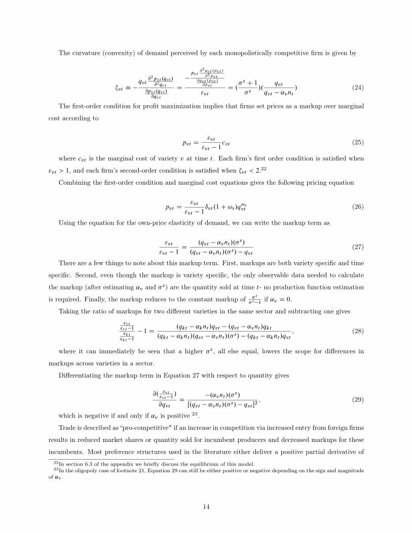
"vt > 1, and each firm’s second-order condition is satisfied when �vt < 2.22

Combining the first-order condition and marginal cost equations gives the following pricing equation

pvt D"vt

"vt � 1ıvt .1C !s/q

!svt (26)

Using the equation for the own-price elasticity of demand, we can write the markup term as

"vt

"vt � 1D

.qvt � ˛vnt /.�s/

.qvt � ˛vnt /.� s/ � qvt(27)

There are a few things to note about this markup term. First, markups are both variety specific and time

specific. Second, even though the markup is variety specific, the only observable data needed to calculate

the markup (after estimating ˛v and � s) are the quantity sold at time t - no production function estimation

is required. Finally, the markup reduces to the constant markup of �s

�s�1if ˛v D 0.

Taking the ratio of markups for two different varieties in the same sector and subtracting one gives

"vt"vt�1"kt"kt�1

� 1 D.qkt � ˛knt /qvt � .qvt � ˛vnt /qkt

.qkt � ˛knt /.qvt � ˛vnt /.� s/ � .qkt � ˛knt /qvt; (28)

where it can immediately be seen that a higher � s, all else equal, lowers the scope for differences in

markups across varieties in a sector.

Differentiating the markup term in Equation 27 with respect to quantity gives

@. "vt"vt�1

/

@qvtD

�.˛vnt /.�s/

Œ.qvt � ˛vnt /.� s/ � qvt �2; (29)

which is negative if and only if ˛v is positive 23.

Trade is described as “pro-competitive" if an increase in competition via increased entry from foreign firms

results in reduced market shares or quantity sold for incumbent producers and decreased markups for these

incumbents. Most preference structures used in the literature either deliver a positive partial derivative of22In section 6.3 of the appendix we briefly discuss the equilibrium of this model.23In the oligopoly case of footnote 21, Equation 29 can still be either positive or negative depending on the sign and magnitude

of ˛v .

14

markups with respect to quantity or (as in the CES case) no change in markups at all. However, as Equation

29 shows, rather than assuming these effects, estimating ˛v allows us to test whether trade is pro-competitive,

anti-competitive, or neither.24

All of these cases are possible in general, as highlighted in recent theory (Krugman (1979), Zhelobodko

et al. (2012), Mrázová and Neary (2017), Parenti et al. (2017), Dhingra and Morrow (forthcoming)). As can

be seen from differentiating the markup term, firm v’s markup is increasing in its quantity sold if ˛v < 0,

is decreasing in its quantity sold if ˛v > 0, and is constant if ˛v D 0. Standard monopolistic competition

models used in the trade literature based on demand systems such as Almost Ideal Demand or Translog

(Feenstra and Weinstein (2017)), Linear demand (Melitz and Ottaviano (2008)), Logit demand (Fajgelbaum

et al. (2011)), and CARA demand (Behrens and Murata (2007)) do not feature anti-competitive effects from

opening to trade. Additionally, trade models based on CES demand with oligopolistic competition (Atkeson

and Burstein (2008), Holmes et al. (2014), De Blas and Russ (2015), Edmond et al. (2015)) also have the

feature that larger market share implies larger market power, and thus successful import penetration must

have pro-competitive effects in these models.

4 Empirical strategy

In this section, we describe our strategy for recovering the deep parameters of the model laid out above,

using U.S. import data from 1998 to 2014. Importantly, we can estimate the parameters of the above partial

equilibrium model without relying on assumptions about the distribution of firm productivity or a full general

equilibrium framework.

Our estimation will proceed in two stages. In the first stage, we will estimate the parameters of the

variety demand functions at the aggregate market level. To address endogeneity concerns, we extend the

Feenstra (1994) approach of identification via heteroskedasticity to estimate the model directly from the

aggregate data on the universe of goods suppliers exporting to the United States. As will be made clear, the

only observable data needed are variety-level prices and sales.

In the second stage, we will estimate the parameters of the sectoral demand functions at the household

level. We do this by supplementing the import data with additional data on the sectoral composition of

the consumption baskets of different income groups from the BLS Consumer Expenditure Survey. To deal

with possible endogeneity, we develop an instrumental variables strategy for this setting. These two stages

of estimation will recover all of the parameters of our model, which, when combined with the microdata,

allow us to construct household-level and aggregate import price indexes.24In the empirical section, we are only using foreign producer data, so, in our context, incumbents should be interpreted as

producers already exporting to the United States. This is a data constraint, not a theoretical one.

15

4.1 Estimation Stage One

While the theory is written to accommodate arbitrarily different ˛’s for every variety, we will specify the

following empirical specification for this parameter:

˛v D1

n1998

hˇCs min

t.qvt j qvt > 0/

ifor v 2 GCs ; (30)

and

˛v D1

n1998

hˇEs min

t.qvt j qvt > 0/

ifor v 2 GEs ; (31)

where ˛v is the subsistence quantity required for variety v, n1998 is the number of households in 1998,

GCs is the set of varieties in sector s that constantly have positive quantities sold throughout the sample

period, GEs is the set of varieties in sector s that enter or exit (e.g., have zero quantity sold) at some point

during the sample period, and ˇjs is the parameter to be estimated that potentially differs across the two

sets of varieties for sector s. We require that ˇEs � 0 and ˇCs < 1. These restrictions satisfy the parameter

restrictions on ˛v required for regularity to hold for all our observations of prices and expenditure.

As a simple example to fix the intuition for this specification, consider the case of ˇCs D 1. In this case, the

total subsistence quantity of variety v sold in 1998 (˛vn1998) is simply the minimum quantity observed in the

import data, and therefore each household consumes mint .qvt j qvt>0/n1998

for subsistence. The total subsistence

quantity sold in any other year t , again in the case of ˇCs D 1, is given by ˛vnt D ntn1998

Œmint .qvt j qvt > 0/�.

For each sector, there are four deep parameters to be estimated: � s, ˇCs , ˇEs , and !s. Conditional on

estimating these parameters, the remaining variety-level unobservables of ˛v (subsistence quantities), 'vt

(demand shifters), ıvt (cost shifters), "vt"vt�1

(markups), and cvt (marginal costs) can be recovered from the

model’s structure given the data on prices and sales.25

To estimate these parameters, we extend the Feenstra (1994) approach of identification via heteroskedas-

ticity to our framework. Our extension is similar in spirit to the approach in Feenstra and Weinstein (2017).

Identification via heteroskedasticity has also been proposed in other recent papers (Rigobon (2003), Lewbel

(2012)).

Start from the variety-level demand expression in Equation 17. Multiplying both sides by pvt , taking

logs, taking the time difference and difference relative to another variety k in the same sector s gives

�k;t ln.pvtqvt � ˛vntpvt / D .1 � �s/�k;t ln.pvt /C �vt ; (32)

where�k;t refers to the double difference and the unobserved error term is �vt D .1 � � s/�4t ln'kt �4t ln'vt

�,

where 4t refers to a single difference across time periods.

Next, we work with the variety-level pricing expression in Equation 26. Multiplying both sides by p!svt ,

taking logs, and double-differencing as before gives25The number of U.S. households in a given year, nt , is available in public data from the U.S. Census Bureau.

16

�k;t lnpvt D!s

1C !s�k;t ln.pvtqvt /C

1

1C !s�k;t ln.

"vt

"vt � 1/C �vt ; (33)

where the unobserved error term is �vt D 11C!s

�4t ln ıvt �4t ln ıkt

�.

As in Feenstra (1994), the orthogonality condition for each variety is then defined as

G.ˇs/ D ET Œxvt .ˇs/� D 0 (34)

where ˇs D

0BB@� s

ˇCsˇEs!s

1CCA and xvt D �vt�vt .

This condition assumes the orthogonality of the idiosyncratic demand and supply shocks at the variety

level after variety and sector-time fixed effects have been differenced out. This orthogonality is plausible

because in addition to the fixed effects, we have also removed variation in prices due to markup variation and

movements along upward-sloping supply curves. The remaining supply shocks take the form of idiosyncratic

shifts in the intercept of the variety-level supply curve and are unlikely to be correlated with idiosyncratic

shifts in the intercept of the variety-level demand curve26.

For each sector s, stack the orthogonality conditions to form the GMM objective function

Os D argmin

ˇs

˚G�.ˇs/

0WG�.ˇs/

(35)

where G�.ˇs/ is the sample counterpart of G.ˇs/ stacked over all varieties in sector s and W is a positive

definite weighting matrix. Following Broda and Weinstein (2010), we give more weight to varieties that are

present in the data for longer time periods and sell larger quantities27. As can be seen from the estimating

equation above, the necessary observables to estimate the model are supplier-product quantities qvt and sales

pvtqvt . Supplier-product prices pvt can be obtained by dividing revenues by quantities to form unit values.

To see how the parameters are identified, rewrite the orthogonality condition that holds for each variety

and rearrange to get

ETŒ.�k;t lnpvt /2� D

!s

.1C !s/ETŒ�

k;t ln.pvtqvt /�k;t lnpvt �

�1

� s � 1ETŒ�

k;t lnpvt�k;t ln.pvtqvt � ˛vntpvt /�

C!s

.1C !s/.� s � 1/ETŒ�

k;t ln.pvtqvt /�k;t ln.pvtqvt � ˛vntpvt /� (36)

C1

.1C !s/ETŒ�

k;t lnpvt�k;t ln."vt

"vt � 1/�

C1

.1C !s/.� s � 1/ETŒ�

k;t ln.pvtqvt � ˛vntpvt /�k;t ln.

"vt

"vt � 1/�

26In a robustness exercise reported below, we show that our estimates do not change very much when we only estimate using asample of multi-variety firms, and take differences relative to another variety within the same firm, in order to remove firm-timefixed effects from the supply and demand error terms.

27Varieties with larger import volumes are expected to have less measurement error in their unit values.

17

This estimating equation shows the importance of heteroskedasticity. If the variances and covariances

in this equation are the same across the different varieties in a given sector, then there is not identification.

However, if the variances and covariances differ across varieties, then pooling the observations of these

moments across varieties in a sector allows for identification of the four common sector-level parameters, so

long as there more varieties in the sector than parameters.

Finally, at this point we recover the variety-level demand shifters. In the spirit of Redding and Weinstein

(2016), we normalize the demand shifter for the geometric average firm-product to be one for all time periods.

Thus, we normalize e'kt D e'k D 1 across firm-products, where the tilde denotes the geometric average. The

demand shifters for all firm-products can be computed using Equation 17 in differences to get the following

expression

'vt D expfln.pvtqvt � ˛vntpvt / � ln.epktqkt � ˛kntpkt /C .� s � 1/.lnpvt � lnepkt /

� s � 1g; (37)

where A.pktqkt � ˛kntpkt / is the geometric average of .pktqkt � ˛kntpkt / across varieties in the sector at

time t .

4.2 Estimation Stage Two

Given the previously estimated parameters, we can now estimate � in the following way. First, we must

construct Yhst , the expenditure on imports by HS4 sector s for household h. We leave the specific details to

the data section, but broadly, we construct the variable using the BLS Consumer Expenditure Survey and

the trade data. Then, starting from the household sector-level demand expression in Equation 7, take the

time difference and difference relative to another sector k bought by the same household h. This double-

differencing gives

�k;t ln.Yhst �Xv2Gs

˛vpvt / D .1 � �/�k;t ln.Pst /C �hst ; (38)

where �hst D .� � 1/��k;t ln'hst

�. We can construct the objects that enter this equation using our

previous parameters and the data. We then form our estimating equation by pooling the double-differenced

observations across households, sectors, and time.

We expect that running Ordinary Least Squares on the above equation would probably not produce

a consistent estimate of � , because of potential endogeneity bias from a possible correlation between the

sectoral price index and the error term. To address this potential issue, we pursue an instrumental variables

approach as in Hottman et al. (2016). Note that, as in section 3.2.5, the change in the log of the sectoral

price index can be linearly decomposed into four terms as follows:

�k;t lnPst D �k;t .

1

N vst

Xv2Gst

lnpvt / ��k;t .

1

N vst

Xv2Gst

ln'vt / ��k;t 1

�S � 1lnN v

st ��k;t 1

�S � 1ln.

1

N vst

Xv2Gst

.pvt'vt/1��

S

D.pvt'vt/1��

S

/;

18

We use the fourth term on the right-hand side, which measures the change in dispersion in quality-

adjusted variety-level prices within a sector, as an instrument for the change in the price index term when

we estimate Equation 38.

Given an estimate of � , we can then solve for the household-specific sectoral demand shifters ('hst ),

which can be done by normalizing e'hkt D e'hk D 1 across sectors and using Equation 7 in differences to

derive

'hst D expfln.Yhst �

Pv2Gs

˛vpvt / � ln.BYhkt �Pv2Gk˛vpvt /C .� � 1/.lnPst � lnePkt /

.� � 1/g (39)

4.3 Data4.3.1 Trade Data

The main data come from the Linked-Longitudinal Firm Trade Transaction Database (LFTTD), which

is collected by U.S. Customs and Border Protection and maintained by the U.S. Census Bureau. Every

transaction in which a U.S. company imports or exports a product requires the filing of Form 7501 with

U.S. Customs and Border Protection, and the LFTTD contains the information from each of these forms.28

There are typically close to 40 million transactions per year.

We utilize the import data from 1998 to 2014, which includes the quantity and value exchanged for each

transaction, Harmonized System (HS) 10 product classification, date of import and export, port information,

country of origin, and a code identifying the foreign supplier. Known as the manufacturing ID, or MID,

the foreign partner identifier contains limited information on the name, address, and city of the foreign

supplier.29 Monarch (2014) and Kamal and Monarch (n.d.) find substantial support for the use of the MID

as a reliable, unique identifier, both over time and in the cross section. Pierce and Schott (2012), Kamal and

Sundaram (2016), Eaton et al. (2014), Heise (2015), and Redding and Weinstein (2017) have all used this

exporter identifier, and Redding and Weinstein (2017) also show that many of the salient features associated

with exporting activity (such as the prevalence of multi-product firms and high rates of product and firm

turnover) are replicated for MID-identified exporters.

We build on the methods of Bernard et al. (2009) for cleaning the LFTTD. Specifically, we drop all

transactions with imputed quantities or values (which are typically very low-value transactions) or converted

quantities or values. We also drop all observations without a valid U.S. firm identifier. After making these

reductions, the average year has close to 2.6 million imported varieties. Figure 1 presents a snapshot of

the number of varieties over different years in our sample- interestingly, the number of varieties increases

dramatically between 1998 and 2007 before declining, rising, and declining again in the latter half of our

time period.28Approximately 80 to 85 percent of these customs forms are filled out electronically (Kamal and Krizan (2012)).29Specifically, the MID contains the first three letters of the producer’s city, six characters taken from the producer’s name,

up to four numeric characters taken from its address, and the ISO2 code for the country of origin.

19

Figure 1: Number of Imported Varieties in the U.S., 1998-2014

1998 1999 2000 2001 2002 2003 2004 2005 2006 2007 2008 2009 2010 2011 2012 2013 20142,000,000

2,200,000

2,400,000

2,600,000

2,800,000

3,000,000

3,200,000

This pattern is new to the literature, so we check it against a number of other similar measures of variety.

First, we compare this number to a more traditional definition of a variety in Figure 2 using publicly available

Census data on the number of country-HS combinations imported by the U.S.30 Although growth is more

muted than in the more disaggregated case (as there are typically multiple suppliers per country), the overall

contour is also very similar, with the exception of the change from 2013 to 2014. Second, motivated by the

potential for changes in HS codes over time (as documented by Pierce and Schott (2009)) to affect our

results, we confirm that this pattern holds even when only using those HS codes that are present in all years

of the data, defining a variety as a supplier in a continuing HS code (the yellow line) and a country in a

continuing HS code (the orange line). Correcting for entering and exiting HS codes does cause the level of

varieties to shrink by close to one-third, but does little to change the time series pattern of the respective

variety measures.

The first estimation stage entails estimating Equation 36 using the trade data. The estimation is per-

formed on a reduced sample of varieties, as a large number of supplier-HS10 combinations only appear once.

Thus, for our cleaned sample, we use only those varieties that are present for six or more years of data.

Furthermore, as Equation 36 relies on double-differenced price and sales terms as components, we winsorize

by dropping double-differenced variety price and sales changes that are below the 1st percentile and above

the 99th percentile. We also drop any HS4 sector that features fewer than 30 varieties over our 17 years of

data. Note that with the exception of our parameter estimation sample, all our results will use the universe

of goods varieties in the U.S. import data.

We run our estimation routine on each HS4 sector where there are enough observations to do so, which30These data are described in Schott (2008) and are available from http://faculty.som.yale.edu/peterschott/sub_

international.htm.

20

Figure 2: Number of Imported Varieties in the U.S., relative to 1998

1

1.1

1.2

1.3

1.4

1.5

1998 1999 2000 2001 2002 2003 2004 2005 2006 2007 2008 2009 2010 2011 2012 2013 2014

Supplier‐HS Varieties Supplier‐Continuing HS Varieties

Country‐HS Varieties Country‐Continuing HS Varieties

amounts to 980 HS4 sectors and over 95% of total U.S. goods imports. The parameters are estimated using

a nonlinear solver to solve the GMM problem described above for each of 980 HS4 sectors. We directly

impose constraints on this nonlinear estimation31. Our approach contrasts with the two-step process of

Broda and Weinstein (2006) and the related literature, which involves estimating parameters from the

unconstrained GMM problem in the first step and then conducting a grid search when the parameters from

the unconstrained estimation take implausible values.

4.3.2 Consumer Expenditure Survey Data

The next step is to move to estimating the sectoral demand equations at the household level. Here we present

the detailed procedure for constructing the household-specific expenditure on imports in an HS4 sector, Yhst .

The BLS Consumer Expenditure Survey (CE) public data provides information on how 10 income deciles

allocate their expenditure across different CE categories, beginning in 2014 (prior years only report expendi-

ture by quintiles)32. The CE is the data that underlie the category expenditure weights in the U.S. Consumer

Price Index. In order to utilize the decile expenditure information along with our parameters estimated at

the HS4 level, we undertake the following steps:31We impose the following constraints: "vt � 1:01, !s � 0, �vt � 1:99, ˇEs � 0, ˇ

Cs < 1, and khv < ˛v , the last of which is

the condition defined in the appendix.32The public-use microdata has income top-coding above the 6th decile, so we cannot use this data to calculate decile-level

expenditure shares for earlier years. In principle, we could use the non-public microdata to produce decile-level tables prior to2014.

21

1. Begin with public U.S. Census Bureau estimates for income levels for each decile and year, 1998 to

2014.

2. Construct expenditure-to-income (EI) ratios for each income level estimate in Step 1 using public data

from the CE in every year.

3. Apply the EI ratios to the Census income numbers by decile to obtain expenditure in every year for

every decile.

4. Apply the 2014 decile-specific expenditure shares across CE categories to each year’s decile total ex-

penditure to get decile-specific expenditure on each CE category.

5. Concord the CE categories to HS4 codes to get decile-specific expenditure on each HS4 category.

6. Apply the import share in domestic absorption for each year to create decile-specific imported expen-

diture in each HS4 category.

For Step 2, we take income levels from Census data and construct expenditure-to-income ratios using

the appropriate annual income-group from the BLS Consumer Expenditure Survey. For example, the first

income decile had an income of $14,070 in 1998, and the CE for 1998 indicates that people who earned

between $10,000 and $15,000 had expenditures equal to 1.613 of their income, on average, so we impute

total expenditure in 1998 to be $22,691.64. We generate total expenditures by applying these EI ratios to

the income data by decile in this manner (Step 3)- the implied expenditure numbers appear reasonably free

from large year-to-year swings.33 After this, we apply the decile-specific category expenditure shares from

2014 to each of these implied total decile expenditure numbers (Step 4). This is a workaround to the fact

that the BLS only provides decile-specific total expenditure and category expenditure shares for 2014. When

we look at earlier years, we find that the category expenditure shares by quintile do not change significantly

from 1998 to 201334.

For Step 5, we use a concordance between the categories in the CE and Harmonized System categories

developed by Furman et al. (2017).35 An important fact to note here is that only about 20% of HS4 sectors

can be found in consumer expenditures- the rest are intermediate inputs. In the end, we will use 228 HS4

sectors in the household price indexes. Although this may appear small, we find that 54.6% of total U.S.

goods import value is in HS4 categories that can be concorded to the CE. Additionally, 361 of the 787 total

expenditure categories in the CE can be linked to an imported HS4 category.

Step 6 entails converting total HS4 expenditure into imported HS4 expenditure. To do this, we multiply

by the sectoral import share in domestic absorption for each year, which is defined as in Feenstra and

Weinstein (2017). Household-specific expenditure on imports from sector s are given by33The expenditure numbers are included in Table 16 in the Appendix.34For example, using the expenditure shares of the broad CE categories (Food, Housing, Apparel, Transportation, Healthcare,

and Entertainment) we find a correlation between the 1998 quintile shares and the 2013 quintile shares of 0.9933.35In cases where one CE category maps into multiple HS4 categories, we use the share of total U.S. import expenditure to

allocate spending across HS4s.

22

Yhst D Ehst .Ms;t

Gs;t �Xs;t CMs;t

/; (40)

where Ehst is the sector-level expenditure by household h derived in Step 5, Ms;t is the nominal value of

U.S. imports in sector s; Gs;t is the nominal value of U.S. production in sector s; and Xs;t is the nominal

value of U.S. exports in sector s. We use total sectoral output data from the BEA to construct Gs;t , and

aggregate imports and exports from the LFTTD to construct Ms;t and Xs;t .36 Also, to clarify notation,

summing Yhst across sectors will result in total expenditure on imports, not total expenditure in the CE,

which we will refer to as TotExpht . Note that although EhstTotExpht

will be constant over time by construction

(since we only have CE decile shares for 2014), sector s’s share of household h’s import basket ( YhstPs Yhst

)

will not be constant over time because sectoral import shares in domestic absorption have different sectoral

trends37.

We find several interesting facts from our Yhst calculation.38 First, the share of imports in total expen-

diture (i.e.,Ps Yhst

TotExpht) does not differ much across income groups: we find that in 2014, the share of imports

in actual expenditure averaged about 10% across deciles, with a standard deviation of 0.5 percentage points.

Thus, any differences in import price indexes across income groups can be meaningfully compared because

there are small differences in shares of imports in consumption. Table 1 shows the share of total expenditure

on imports across different deciles in 1998 and 2014. Interestingly, there is not much variation across deciles

in the cross section, but the share of spending on imports does increase over our time period.

Table 1: Share of Expenditure on Imports by U.S. Decile of Income, 1998 and 2014 (%)

Year 1st Decile 2nd Decile 4th Decile 5th Decile 6th Decile 8th Decile 9th Decile1998 6.49 6.58 6.35 6.99 7.49 7.01 7.052014 9.96 9.22 9.24 10.05 10.63 10.02 10.06

Second, non-homotheticity across broad imported sectors is evident from the data. As one example, for

each household, we create the ratio of expenditure on CE-HS4 concorded imported food as a share of total

CE-HS4 concorded imports:Ps2Food Yhst=

Ps Yhst . Figure 3 shows the differences across income deciles for

spending on imported food in 2014: there are indeed large differences across income groups.36Gs;t is constructed using a concordance between NAICS codes and HS codes. In cases where one NAICS code maps into

multiple HS4 categories, we use the share of U.S. exports in each sector to allocate production across HS4s.37When we compute the percent change between 1998 and 2014 for each sector’s share of each decile’s imported consumption

( YhstPs Yhst

), we find that across all decile-sectors the 25th percentile is a 27.6% decrease in share, the median is a 7.1% increasein share, and the 75th percentile is a 85.8% increase in share.

38The calculations in section 4.3.2 rely on a version of Yhst constructed using public trade data for Ms;t and Xs;t .

23

Figure 3: Imported Food as a Share of Imported Consumption by Income Decile in 2014

18.0

20.0

22.0

24.0

26.0

28.0

30.0

32.0

1 2 4 5 6 8 9

Imported Food's Share of Income Decile's Imported Consumption

Another way to show this fact is to compare expenditure in HS4 categories as a share of total HS4

expenditures (i.e., YhstPs Yhst

�YhstYht

) across income deciles. Table 2 presents summary statistics across HS4

categories, weighted by expenditure in an HS4. Again, we find meaningful variation across deciles. Panel

(a) of Table 2 presents summary statistics for the ratio of Decile 9 expenditure shares over Decile 1 expen-

diture shares in 2014 (Y9st=Y9tY1st=Y1t

). The 25th and 75th percentiles demonstrate a wide range of differences in

expenditure shares across these deciles. Panels (b)-(d) show similar findings for other decile comparisons in

2014.

Table 2: Summary Statistics for Decile-to-Decile Expenditure Share Ratios in 2014

(a) Decile 9 to Decile 1 (Y9st=Y9tY1st=Y1t

)

10th Percentile 25th Percentile Median 75th Percentile 90th Percentile0.6101 0.7313 1.0068 1.1271 1.7832

(b) Decile 9 to Decile 5 (Y9st=Y9tY5st=Y5t

)

10th Percentile 25th Percentile Median 75th Percentile 90th Percentile0.7370 0.8644 0.8918 1.1753 1.4986

(c) Decile 2 to Decile 5 (Y2st=Y2tY5st=Y5t

)

10th Percentile 25th Percentile Median 75th Percentile 90th Percentile0.2735 0.9220 1.1292 1.3089 1.4230

(d) Decile 2 to Decile 1 (Y2st=Y2tY1st=Y1t

)

10th Percentile 25th Percentile Median 75th Percentile 90th Percentile0.6228 0.9254 1.0806 1.1438 1.3301

With Yhst constructed, we work with Equation 38 to obtain � and 'hst , giving us everything we need to

24

make the household-specific import price indexes.

5 Estimation Results

We use the supplier-level data to estimate the sector-level parameters of the model and use them to construct

import price indexes in the aggregate and for different income groups.

5.1 Parameter Estimates

We start with estimates of � s, which is the sectoral-level elasticity of substitution that is comparable to

estimates from Broda and Weinstein (2006). In all sectors our estimate of � s is statistically different from

zero at the 5 percent level or better. We also find that � s > 1 in all sectors. Across sectors, our estimates

of the elasticity of substitution have a median of 4.9, squarely in line with earlier findings for U.S. imports 39.

Table 3: Summary of � s

10% Median 90%3.06 4.93 8.59

Table 4 reports our estimate of � , which is the aggregate-level elasticity of substitution (across consumer

goods). The first column shows the OLS result from our estimating equation, while the second column

reports the Instrumental Variable (IV) estimate. As would be expected from the presence of an endogeneity

bias in this setting, the OLS estimate is biased toward zero. The IV estimate of � is about 2.8, with a 95

percent confidence interval between 2.6 and about 3. Note that most papers in the literature assume that

� D 1, making upper-tier utility Cobb-Douglas. Redding and Weinstein (2017) also estimates the elasticity

of substitution across U.S. HS4 import sectors from 1997-2011, and reports an estimate of 1.36.

Table 4: Estimates of �

OLS estimate IV estimate IV 95% C.I.0.82 2.78 (2.60 - 2.97)

Another parameter that corresponds with earlier work is the elasticity of marginal cost with respect to

output, !s. In all but a handful of sectors our estimate of !s is statistically different from zero at the 5

percent level or better. Again, our estimated parameters are in line with previous work40.39For comparison, starting with the Broda and Weinstein (2006) estimates of �s at the HS10 level for U.S. imports from

1990-2001, and collapsing to the HS4 level by taking the mean across HS10 estimates, then the 10th percentile value of �s is1.91, the median is 4.46, and the 90th percentile is 22.5.

40For comparison, Soderbery (2015) reports hybrid Feenstra estimates of !s for U.S. imports at the HS8 level from 1993 to2007, which range from 0.03 at the 25th percentile to 1.06 at the 75th percentile, with a median of 0.26. After collapsing to theHS4 level by taking the median of !s across HS8 estimates in Soderbery (2015), then the 10th percentile value of !s is 0.03,the median is 0.30, and the 90th percentile is 14.09.

25

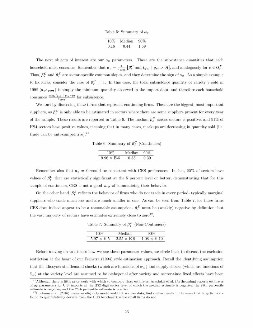
Table 5: Summary of !s

10% Median 90%0.16 0.44 1.59

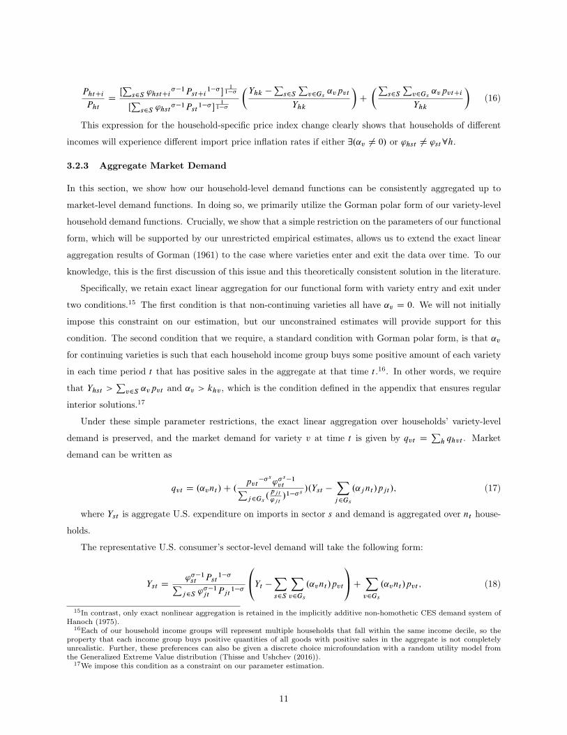
The next objects of interest are our ˛v parameters. These are the subsistence quantities that each

household must consume. Remember that ˛v D 1n1998

�ˇCs mint .qvt j qvt > 0/

�, and analogously for v 2 GEs .

Thus, ˇCs and ˇEs are sector-specific common slopes, and they determine the sign of ˛v. As a simple example

to fix ideas, consider the case of ˇCs D 1. In this case, the total subsistence quantity of variety v sold in

1998 (˛vn1998) is simply the minimum quantity observed in the import data, and therefore each household

consumes mint .qvt j qvt>0/n1998

for subsistence.

We start by discussing the ˛ terms that represent continuing firms. These are the biggest, most important

suppliers, as ˇCs is only able to be estimated in sectors where there are some suppliers present for every year

of the sample. These results are reported in Table 6. The median ˇCs across sectors is positive, and 91% of

HS4 sectors have positive values, meaning that in many cases, markups are decreasing in quantity sold (i.e.

trade can be anti-competitive).41

Table 6: Summary of ˇCs (Continuers)

10% Median 90%9.96 � E-5 0.33 0.39

Remember also that ˛v D 0 would be consistent with CES preferences. In fact, 85% of sectors have

values of ˇCs that are statistically significant at the 5 percent level or better, demonstrating that for this

sample of continuers, CES is not a good way of summarizing their behavior.

On the other hand, ˇEs reflects the behavior of firms who do not trade in every period- typically marginal

suppliers who trade much less and are much smaller in size. As can be seen from Table 7, for these firms

CES does indeed appear to be a reasonable assumption- ˇEs must be (weakly) negative by definition, but

the vast majority of sectors have estimates extremely close to zero42.

Table 7: Summary of ˇEs (Non-Continuers)

10% Median 90%-5.97 � E-5 -2.55 � E-9 -1.08 � E-10

Before moving on to discuss how we use these parameter values, we circle back to discuss the exclusion

restriction at the heart of our Feenstra (1994) style estimation approach. Recall the identifying assumption

that the idiosyncratic demand shocks (which are functions of 'vt ) and supply shocks (which are functions of

ıvt ) at the variety level are assumed to be orthogonal after variety and sector-time fixed effects have been41Although there is little prior work with which to compare these estimates, Arkolakis et al. (forthcoming) reports estimates

of ˛v parameters for U.S. imports at the HS2 digit sector level of which the median estimate is negative, the 25th percentileestimate is negative, and the 75th percentile estimate is positive.

42Hottman et al. (2016), using an oligopoly model and U.S. scanner data, find similar results in the sense that large firms arefound to quantitatively deviate from the CES benchmark while small firms do not.

26

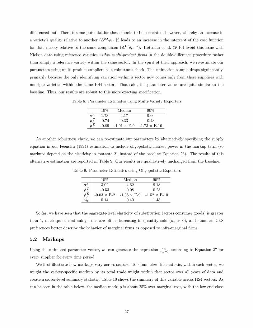
differenced out. There is some potential for these shocks to be correlated, however, whereby an increase in

a variety’s quality relative to another (�k;t'vt ") leads to an increase in the intercept of the cost function

for that variety relative to the same comparison (�k;tıvt "). Hottman et al. (2016) avoid this issue with

Nielsen data using reference varieties within multi-product firms in the double-difference procedure rather

than simply a reference variety within the same sector. In the spirit of their approach, we re-estimate our

parameters using multi-product suppliers as a robustness check. The estimation sample drops significantly,

primarily because the only identifying variation within a sector now comes only from those suppliers with

multiple varieties within the same HS4 sector. That said, the parameter values are quite similar to the

baseline. Thus, our results are robust to this more exacting specification.

Table 8: Parameter Estimates using Multi-Variety Exporters

10% Median 90%� s 1.73 4.17 9.60ˇCs -0.74 0.33 0.43ˇEs -0.89 -1.91 � E-9 -1.73 � E-10

As another robustness check, we can re-estimate our parameters by alternatively specifying the supply

equation in our Feenstra (1994) estimation to include oligopolistic market power in the markup term (so

markups depend on the elasticity in footnote 21 instead of the baseline Equation 23). The results of this

alternative estimation are reported in Table 9. Our results are qualitatively unchanged from the baseline.

Table 9: Parameter Estimates using Oligopolistic Exporters

10% Median 90%� s 3.02 4.62 9.18ˇCs -0.53 0.08 0.23ˇEs -0.03 � E-2 -1.36 � E-9 -1.52 � E-10!s 0.14 0.40 1.48

So far, we have seen that the aggregate-level elasticity of substitution (across consumer goods) is greater

than 1, markups of continuing firms are often decreasing in quantity sold (˛v > 0), and standard CES

preferences better describe the behavior of marginal firms as opposed to infra-marginal firms.

5.2 Markups

Using the estimated parameter vector, we can generate the expression "vt"vt�1

according to Equation 27 for

every supplier for every time period.

We first illustrate how markups vary across sectors. To summarize this statistic, within each sector, we

weight the variety-specific markup by its total trade weight within that sector over all years of data and

create a sector-level summary statistic. Table 10 shows the summary of this variable across HS4 sectors. As

can be seen in the table below, the median markup is about 25% over marginal cost, with the low end close

27

to 13% and the high end at 48%.43

Table 10: Markup Variation across HS4 Sectors ( "vt"vt�1

)

10% Median 90%Sales-Weighted Average 1.132 1.250 1.482

We can also how see the typical markup changes over time. Here we simply take the sales-weighted

median markup over all varieties sold in each year and track how this median moves over time. As can be

seen in Table 11, the median markup declined over the first half of the sample before flattening out from 2010

onward. Given our earlier results showing that markups are often decreasing in quantity sold, these markup

declines in the early part of our sample likely reflect a large increase in imports in early years, followed by a

leveling off.44

Table 11: Median Markup Over Time (Sales-Weighted)

Year 1998 2002 2006 2010 2014Markup 1.235 1.226 1.215 1.215 1.215Markup- Continuers 1.234 1.174 1.134 1.130 1.132

For robustness, we also report the markup results implied by the oligopoly specification from Table 9.

While markups are slightly higher in the oligopoly case, the results in terms of how the average markup

changes over time are unchanged from the baseline. This can be seen in Table 12 below.

Table 12: Median Markup Over Time (Sales-Weighted): Oligopoly case

Year 1998 2002 2006 2010 2014Markup 1.256 1.251 1.237 1.235 1.235Markup- Continuers 1.288 1.260 1.224 1.180 1.192

5.3 Aggregate Import Price Index

With our parameter estimates in hand, we can calculate the aggregate import price index for the United

States from 1998 to 2014. The exercise is similar to that of Broda and Weinstein (2006) but with the two

key differences that prices (and thus varieties) are supplier specific and that the preferences used here are a

more flexible, non-homothetic generalization of the CES preferences used in their study. We calculate the

aggregate import price index for each year from 1999 to 2014, with 1998 as the reference year.

5.3.1 Baseline Results

The results are shown in Figure 4. The value of the price index in each year is also reported in table form in

the Appendix. The dashed lines in the figure represent error bands, computed by recalculating the aggregate43For comparison, Feenstra and Weinstein (2017) estimate a median markup across HS4 digit U.S. import sectors in 2005 of

30% over marginal cost.44Feenstra and Weinstein (2017) also estimate that markups have declined in U.S. import sectors between 1992 and 2005.

28

import price index using values of � that represent the 95% thresholds for this parameter shown in Table 4.

We find a U-shaped pattern: by 2006, import prices were nearly 12% lower than in 1998. However, by 2014,

prices are about 8% higher than in 1998. The fall in the import price index in the early part of the period

is consistent with the large increase in the number of foreign varieties observed over this time period as well

as the decrease in median markups.

Figure 4: U.S. Import Price Index, 1998-2014

0.8

0.85

0.9

0.95

1

1.05

1.1

1998 1999 2000 2001 2002 2003 2004 2005 2006 2007 2008 2009 2010 2011 2012 2013 2014

Aggregate Import Price Index

Figure 5 again plots our estimated aggregate import price index from 1998 through 2014, with 1998

normalized to one. For comparison, the figure also plots the BLS All-Commodity Import Price Index, which

is a Laspeyres price index constructed from survey data gathered through the International Price Program.

Interestingly, the decline in our aggregate import price index from 1998-2006 is in contrast with the published

import price index from the BLS, which rises over this time period. Of course, the BLS price index is not

variety adjusted or widely quality adjusted and likely suffers from a substitution bias from the base period

weights used in the Laspeyres formula45.45Our import price index nests a Laspeyres index as a limiting special case when ˛v D 0, 'vt D 'v , 'st D 's , �s ! 0, and

� ! 0, as shown in Redding and Weinstein (2016).

29

Figure 5: U.S. Import Price Indexes, 1998-2014

0.8

0.9

1

1.1

1.2

1.3

1.4

1.5

1.6

1998 1999 2000 2001 2002 2003 2004 2005 2006 2007 2008 2009 2010 2011 2012 2013 2014

Aggregate Import Price Index BLS All‐Commodity Import Price Index

To summarize, we find that our aggregate import price index, with 1998 normalized to 1, was about 1.08

in 2014. For comparison, the All-Commodity Import Price Index from the BLS, which with 1998 normalized

to 1, takes a value of about 1.48 in 2014. The ratio of the two, 1.48/1.08, implies an upward bias in the

Laspeyres import price index over our time period of about 37%, or about 2 percentage points per year46.

5.3.2 Components of the Aggregate Import Price Index

Recall from Equation 21 that we can break down our import price index into a few major components. In

particular, the CES portion of the price index can be written as

ln.ŒXs2S

'��1st Pst1�� �

11�� / D

1

N St

Xs2S

.1

N vst

Xv2Gst

lnpvt /

�1

N St

Xs2S

.1

N vst

Xv2Gst

ln'vt / �1

N St

Xs2S

ln'st

�1

� � 1lnN S

t �1

N St

Xs2S

1

�S � 1lnN v

st (41)

�1

� � 1ln.

1

N St

Xs2S

.Pst'st/1��

3.Pst'st/1��

/ �1

N st

Xs2S

1

�S � 1ln.

1

N vst

Xv2Gst

.pvt'vt/1��

S

4.pvt'vt/1��

S

/:

This equation illustrates how we can consider what factors contributed to the U-shaped trend we observe

in our price index47. For example, we can look at the geometric average of observed variety-level prices,46For comparison, Broda and Weinstein (2006) use a CES aggregate import price index and find an upward bias in the non-

variety-adjusted import price index of 28 percent, or 1.2 percentage points per year over the 1972-2001 time period. Relativeto their exercise, our comparison to the Laspeyres price index includes additional sources of bias such as the substitution bias.

47Since our estimated ˛v terms tend to be very small, the approximation of our price index by the CES-style component onthe left side of Equation 41 is likely to be a very good one.

30

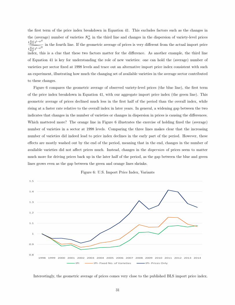
the first term of the price index breakdown in Equation 41. This excludes factors such as the changes in

the (average) number of varieties N vst in the third line and changes in the dispersion of variety-level prices

.pvt'vt

/1��S

3.pvt'vt

/1��S

in the fourth line. If the geometric average of prices is very different from the actual import price

index, this is a clue that these two factors matter for the difference. As another example, the third line

of Equation 41 is key for understanding the role of new varieties: one can hold the (average) number of

varieties per sector fixed at 1998 levels and trace out an alternative import price index consistent with such

an experiment, illustrating how much the changing set of available varieties in the average sector contributed

to these changes.

Figure 6 compares the geometric average of observed variety-level prices (the blue line), the first term

of the price index breakdown in Equation 41, with our aggregate import price index (the green line). This

geometric average of prices declined much less in the first half of the period than the overall index, while

rising at a faster rate relative to the overall index in later years. In general, a widening gap between the two

indicates that changes in the number of varieties or changes in dispersion in prices is causing the differences.

Which mattered more? The orange line in Figure 6 illustrates the exercise of holding fixed the (average)

number of varieties in a sector at 1998 levels. Comparing the three lines makes clear that the increasing

number of varieties did indeed lead to price index declines in the early part of the period. However, these

effects are mostly washed out by the end of the period, meaning that in the end, changes in the number of

available varieties did not affect prices much. Instead, changes in the dispersion of prices seem to matter

much more for driving prices back up in the later half of the period, as the gap between the blue and green

lines grows even as the gap between the green and orange lines shrinks.

Figure 6: U.S. Import Price Index, Variants

1998 1999 2000 2001 2002 2003 2004 2005 2006 2007 2008 2009 2010 2011 2012 2013 20140.8

0.9

1

1.1

1.2

1.3

1.4

1.5

IPI IPI‐ Fixed No. of Varieties IPI‐ Prices Only

Interestingly, the geometric average of prices comes very close to the published BLS import price index.

31

Figure 7 compares the geometric average price index (the blue line) with the price index from the BLS (the

red line) over the 2000 to 2012 period, now setting 2000 to one for both series. Remarkably, the two price

indexes behave very similarly in this subperiod, with the exception that our price index falls significantly

less in 2009 than the BLS price index.

Figure 7: U.S. Import Price Indexes, 2000-2012

2000 2001 2002 2003 2004 2005 2006 2007 2008 2009 2010 2011 20120.9

1

1.1

1.2

1.3

1.4

1.5

IPI‐ Prices Only BLS All‐Commodity Import Price Index

5.3.3 The Role of China

Another interesting question is the extent to which the well-known increase in U.S. trade with China con-

tributed to changes in the aggregate price index. Although our model does not permit a full general equi-

librium accounting of such an exercise, we can plot how the prices of non-Chinese varieties moved over this

time period.48 This comparison can be seen in Figure 8. Beginning in 2002, import price inflation for the

group of non-Chinese varieties rose more than the overall price index, implying a deflationary effect of China

for U.S. consumers. According to our baseline index, overall import inflation was 0.47% annualized between

1998 and 2014, while the non-China import price inflation was 0.73%49.48Not accounting for general equilibrium effects implies that prices and sales of the rest of the world’s varieties would evolve

equally compared with the case with Chinese varieties included.49When we look at the results of the same exercise focusing just on consumer products at the decile level, we will find a

difference in annual average inflation rates of about 0.5 percentage point, which is twice as large as this aggregate result.

32

Figure 8: U.S. Import Price Index, With and Without Chinese Varieties

0.8

0.85

0.9

0.95

1

1.05

1.1

1.15

1998 1999 2000 2001 2002 2003 2004 2005 2006 2007 2008 2009 2010 2011 2012 2013 2014

Import Price Index Import Price Index‐ No China Varieties

5.4 Import Price Inflation Across Consumers5.4.1 Baseline Results

Figure 9 reports import price indexes for selected income deciles over the entirety of 1998 through 2014,

namely the lowest, median, and second-highest deciles of income in the United States.50 The results for these

and other deciles are reported in table form in the appendix. The dashed lines in the figure represent error

bands, computed by recalculating the income-decile specific price indexes using values of � that represent

the 95% thresholds for this parameter above.51

There are several features of Figure 9 to discuss. First, note that the price index for the ninth decile of

income is below the other deciles in every year after 2002. Thus, the higher-income households experienced

less cumulative import price inflation than other households. Second, with the exception of 2009, the price

index for the lowest decile of income was above the other deciles in almost every year after 2002. Therefore,

the lowest-income households experienced the most cumulative import price inflation over this time period.50The U.S. Census Bureau does not disclose income amounts for the third, seventh, or tenth deciles.51Error bands calculated using the 95% thresholds from the nonlinear estimates of the sector level parameters ˇEs and ˇCs

are also extremely tight, and are available upon request.

33

Figure 9: U.S. Import Price Index, 1998-2014, Selected Income Deciles

1998 1999 2000 2001 2002 2003 2004 2005 2006 2007 2008 2009 2010 2011 2012 2013 20140.8

0.85

0.9

0.95

1

1.05

1.1

1.15

1.2

1.25

1.3

1st Income Decile Median Income Decile 9th Income Decile

Figure 9 can be compared with changes in nominal income for different deciles over the same time period.

As can be seen in Figure 10, U.S. Census data on income thresholds indicate that the highest income for a

person in the ninth income decile has risen about 7.5% from 1998 to 2014. At the same time, the highest

income of consumers in the first decile has dropped by about 12.5% 52.

.

Figure 10: Cumulative Percent Change in U.S. Decile Income Thresholds, 1998-2014

‐15.0

‐12.5

‐10.0

‐7.5

‐5.0

‐2.5

0.0

2.5

5.0

7.5

10.0

1998 1999 2000 2001 2002 2003 2004 2005 2006 2007 2008 2009 2010 2011 2012 2013 2014

1st Income Decile Median Income Decile 9th Income Decile

52We report the full set of decile thresholds in Table 18 in the Appendix.

34

Figure 11 shows the average annual change in income thresholds by decile over the 1998 to 2014 period.

Note that decile five is the median decile of income, and we do not report results for deciles three, seven,

or ten. Notably, there is a positive relationship between the decile of income and its average annual income

threshold change over this time period.

Figure 11: Average Annual Income Threshold Change by Decile, 1998-2014

-1.00

-0.80

-0.60

-0.40

-0.20

0.00

0.20

0.40

0.60

1 2 4 5 6 8 9

Income Decile's Change in Income Threshold (A.R.)

Figure 12 plots the import price inflation rates experienced by different deciles over the 1998 to 2014

period. We can see that the lowest-income households experienced the most inflation, while import price

inflation was substantially lower for higher-income deciles. Therefore, we find a negative relationship between

the decile of income and the average annual import price inflation over this time period. Importantly, the

sign of this relationship is the opposite of what we saw in terms of nominal income changes. Thus, changes

in import prices appear to be exacerbating increases in nominal income inequality over this time period.

35

Figure 12: Average Annual Import Price Inflation by Decile, 1998-2014

0.50

0.60

0.70

0.80

0.90

1.00

1.10

1.20

1.30

1.40

1.50

1 2 4 5 6 8 9

Income Decile's Import Price Inflation (A.R.)

5.4.2 Within- vs. Across-Sector Non-Homotheticity

Our model permits both within-sector (through ˛v) and across-sector non-homotheticity (through 'hst ). In

this section, we consider the relative importance of each of these channels to the differences in decile-level

import price inflation described above.

We first set all ˛v terms equal to zero and recalculate the decile-level price indexes. As can be seen from

Figure 13, shutting down within-sector non-homotheticity changes the lines only slightly and does not alter

the qualitative picture that consumers in the lowest income decile experienced the highest level of import

price inflation.

36

Figure 13: U.S. Import Price Index for ˛v D 0, Selected Deciles

0.8

0.85

0.9

0.95

1

1.05

1.1

1.15

1.2

1.25

1.3

1998 1999 2000 2001 2002 2003 2004 2005 2006 2007 2008 2009 2010 2011 2012 2013 2014

1st Income Decile Median Income Decile 9th Income Decile

However, shutting down cross-sector non-homotheticity by setting all household-level sectoral demand

shifters 'hst equal to the sectoral average 'st leads to a very different picture. Figure 14 shows that by

shutting down variation in the sectoral demand shifters across households, import price inflation differences

across deciles collapses to the point of being indistinguishable.53

Figure 14: U.S. Import Price Index for 'hst D 'st , Selected Deciles

0.8

0.85

0.9

0.95

1

1.05

1.1

1.15

1.2

1.25

1998 1999 2000 2001 2002 2003 2004 2005 2006 2007 2008 2009 2010 2011 2012 2013 2014

1st Income Decile Median Income Decile 9th Income Decile

53Individual yearly observations of the index are not exactly equal; they tend to differ by about 0.0001 to 0.0002 percentagepoint.

37

5.4.3 The Role of Different Products

Although we have shown that the total share of income spent on imported products does not differ much

across income deciles, it is still the case that the share of income spent on particular imported products differs

widely across deciles. One particularly useful decomposition is separating out food and energy products

from the overall price index to generate a “core” import price index. As can be seen in Figure 15, this

index preserves many of the same features of the baseline index: a U-shaped pattern for prices, important

differences between deciles, and the ninth decile of income facing the lowest level of import price inflation.

Figure 15: U.S. Import Price Index for “Core" Products, Selected Deciles

1998 2000 2002 2004 2006 2008 2010 2012 20140.75

0.8

0.85

0.9

0.95

1

1.05

1.1

1.15

1st Income Decile Median Income Decile 9th Income Decile

However, the import price index for food and energy (i.e. “Non-Core”) products in Figure 16 looks very

different. Although the richest decile still has the lowest level of inflation, prices for these imported products

rose steadily over the time period. Additionally, there are less stark differences between the median and

lowest-income deciles for non-core products.

38

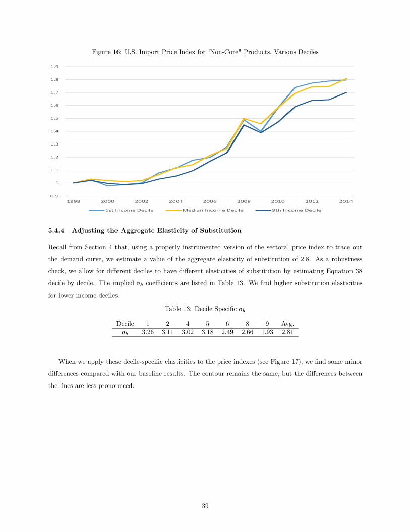
Figure 16: U.S. Import Price Index for “Non-Core" Products, Various Deciles

1998 2000 2002 2004 2006 2008 2010 2012 20140.9

1

1.1

1.2

1.3

1.4

1.5

1.6

1.7

1.8

1.9

1st Income Decile Median Income Decile 9th Income Decile

5.4.4 Adjusting the Aggregate Elasticity of Substitution

Recall from Section 4 that, using a properly instrumented version of the sectoral price index to trace out

the demand curve, we estimate a value of the aggregate elasticity of substitution of 2.8. As a robustness

check, we allow for different deciles to have different elasticities of substitution by estimating Equation 38

decile by decile. The implied �h coefficients are listed in Table 13. We find higher substitution elasticities

for lower-income deciles.

Table 13: Decile Specific �h

Decile 1 2 4 5 6 8 9 Avg.�h 3.26 3.11 3.02 3.18 2.49 2.66 1.93 2.81

When we apply these decile-specific elasticities to the price indexes (see Figure 17), we find some minor

differences compared with our baseline results. The contour remains the same, but the differences between

the lines are less pronounced.

39

Figure 17: U.S. Import Price Index, Decile-Specific �h

1998 2000 2002 2004 2006 2008 2010 2012 20140.8

0.85

0.9

0.95

1

1.05

1.1

1.15

1.2

1.25

1.3

1st Income Decile Median Income Decile 9th Income Decile

Our estimate of � D 2:8 is higher than Redding andWeinstein (2017)’s estimate of 1.36, partly because our

estimation sample for the second stage includes only those sectors that are directly consumed by households,

as is clear from Equation 38. A typical parametrization of the aggregate elasticity of substitution in the

literature would be � D 1, which corresponds to Cobb-Douglas preferences. If we were to adopt a value

of � that is close to the estimate from Redding and Weinstein (2017) and much closer to Cobb-Douglas

preferences, then our price index is changed significantly in magnitude relative to the baseline, as seen in

Figure 18. Differences between income groups are far larger in this case.

Figure 18: U.S. Import Price Index, � D 1:3

1998 1999 2000 2001 2002 2003 2004 2005 2006 2007 2008 2009 2010 2011 2012 2013 20140.5

0.7

0.9

1.1

1.3

1.5

1.7

1.9

2.1

2.3

2.5

1st Income Decile Median Income Decile 9th Income Decile

40

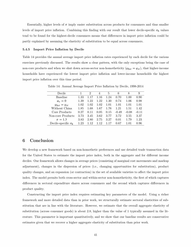
Essentially, higher levels of � imply easier substitution across products for consumers and thus smaller

levels of import price inflation. Combining this finding with our result that lower decile-specific �h values

tend to be found for the highest-decile consumers means that differences in import price inflation could be

partly explained by assuming the elasticity of substitution to be equal across consumers.

5.4.5 Import Price Inflation by Decile

Table 14 provides the annual average import price inflation rates experienced by each decile for the various

exercises previously discussed. The results show a clear pattern, with the only exceptions being the case of

non-core products and when we shut down across-sector non-homotheticity ('hst D 'st ), that higher-income

households have experienced the lowest import price inflation and lower-income households the highest

import price inflation over this time period.

Table 14: Annual Average Import Price Inflation by Decile, 1998-2014

Decile 1 2 4 5 6 8 9Baseline 1.33 1.17 1.16 1.24 0.70 1.00 0.90˛v D 0 1.39 1.22 1.22 1.30 0.74 1.06 0.98

'hst D 'st 1.02 1.02 1.02 1.01 1.01 1.01 1.01Without China 1.85 1.68 1.67 1.76 1.21 1.51 1.42Core Products 0.27 0.11 0.05 0.15 -0.49 -0.08 -0.11

Non-core Products 3.73 3.45 3.62 3.77 3.72 3.55 3.37� D 1:3 3.83 2.80 2.75 3.27 0.01 1.79 1.23

Decile-specific �h 1.23 1.12 1.12 1.17 0.67 1.01 0.96

6 Conclusion

We develop a new framework based on non-homothetic preferences and use detailed trade transaction data

for the United States to estimate the import price index, both in the aggregate and for different income

deciles. Our framework allows changes in average prices (consisting of marginal cost movements and markup

adjustment), changes in the dispersion of prices (i.e., changing opportunities for substitution), product

quality changes, and an expansion (or contraction) in the set of available varieties to affect the import price

index. The model permits both cross-sector and within-sector non-homotheticity, the first of which captures

differences in sectoral expenditure shares across consumers and the second which captures differences in

product quality.

Constructing the import price index requires estimating key parameters of the model. Using a richer

framework and more detailed data than in prior work, we structurally estimate sectoral elasticities of sub-

stitution that are in line with the literature. However, we estimate that the overall aggregate elasticity of

substitution (across consumer goods) is about 2.8, higher than the value of 1 typically assumed in the lit-

erature. This parameter is important quantitatively, and we show that our baseline results are conservative

estimates given that we recover a higher aggregate elasticity of substitution than prior work.

41

We use our parameter estimates and the variety-level universe of goods trade data to construct the

aggregate U.S. import price index. Relative to 1998, we find that aggregate import prices rose about 8%

by 2014. For comparison, the Laspeyres-based BLS import price index, which does not capture substitution

effects or changes in the set of imported varieties, rose by 48% over this time period. Therefore, we estimate

an upward bias in the Laspeyres import price index over our time period of about 37%, or about 2 percentage

points per year.

We also find that developments in U.S. trade over the past two decades have had important distributional

consequences through the consumption channel. In particular, we find that lower-income households experi-

enced the most import price inflation from 1998 to 2014, while the higher-income households experienced the

least import price inflation. In our baseline results, the 1st income decile experienced import price inflation

of about 24% from 1998 to 2014, or about 1.33 percent per year. For comparison, the 9th income decile

only experienced import price inflation of about 15% over that time period, or about 0.90 percent per year.

Therefore, we do not find evidence that the consumption channel has mitigated the distributional effects

of trade that have occurred through the nominal income channel in the United States over the past two

decades. Instead, our results imply that import price changes have exacerbated the increase in nominal in-

come inequality. Our results also indicate that cross-sector non-homotheticity is the key mechanism driving

the differences in import inflation across import groups.

References

Ackerberg, Daniel and Marc Rysman, “Unobserved Product Differentiation in Discrete Choice Models:

Estimating Price Elasticities and Welfare Effects,” RAND Journal of Economics, 2005, 36 (4), 771–788.

Aghion, Philippe, Antonin Bergeaud, Timo Boppart, Peter J. Klenow, and Huiyu Li, “Missing

Growth from Creative Destruction,” NBER Working Paper 24023, 2017.

Aguiar, Mark and Mark Bils, “Has Consumption Inequality Mirrored Income Inequality?,” American

Economic Review, 2015, 105 (9), 2725–2756.

Amiti, Mary, Mi Dai, Robert Feenstra, and John Romalis, “How Did China’s WTO Entry Benefit

U.S. Consumers?,” NBER Working Paper 23487, 2017.

Antràs, Pol, Alonso de Gortari, and Oleg Itskhoki, “Globalization, Inequality, and Welfare,” Journal

of International Economics, 2017, 108, 387–412.

Arkolakis, Costas, Arnaud Costinot, and Andres Rodríguez-Clare, “New Trade Models, Same Old

Gains?,” American Economic Review, 2012, 102 (1), 94–130.

, , David Donaldson, and Andres Rodríguez-Clare, “The Elusive Pro-Competitive Effects of

Trade,” Review of Economic Studies, forthcoming.

42

Atkeson, Andrew and Ariel Burstein, “Pricing to Market, Trade Costs and International Relative

Prices,” American Economic Review, 2008, 98 (5), 1998–2031.

Atkin, David, Benjamin Faber, and Marco Gonzalez-Navarro, “Retail Globalization and Household

Welfare: Evidence from Mexico,” Journal of Political Economy, Forthcoming.

Autor, David H., David Dorn, and Gordon H. Hanson, “The China Shock: Learning from Labor-

Market Adjustment to Large Changes in Trade,” Annual Review of Economics, 2016, 8, 205–240.

Bajari, Patrick and C. Lanier Benkard, “Discrete Choice Models as Structural Models of Demand:

Some Economic Implications of Common Approaches,” Stanford Graduate School of Business Research

Paper 1710, 2003.

Barnett, William, “Recursive Subaggregation and a Generalized Hypocycloidal Demand Model,” Econo-

metrica, 1977, 45 (5), 1117–1136.

Behrens, Kristian and Yasusada Murata, “General Equilibrium Models of Monopolistic Competition:

A New Approach,” Journal of Economic Theory, 2007, 136 (1), 776–787.

and , “Trade, Competition, and Efficiency,” Journal of International Economics, 2012, 87 (1), 1–17.

Bernard, Andrew B., J. Bradford Jensen, and Peter K. Schott, “Importers, Exporters and Multina-

tionals: A Portrait of Firms in the U.S. that Trade Goods,” in “Producer Dynamics: New Evidence from

Micro Data,” University of Chicago Press, 2009, pp. 513–552.

Berner, Richard, “Estimating Consumer Import Demand Equations,” Federal Reserve Board International

Finance Discussion Paper 105, 1977.

Bertoletti, Paolo and Paolo Epifani, “Monopolistic Competition: CES Redux?,” Journal of International

Economics, 2014, 93 (2), 227–238.

Bils, Mark and Peter J. Klenow, “Quantifying Quality Growth,” American Economic Review, 2001, 91

(2), 1006–1030.

Blackorby, Charles, Daniel Primont, and R. Robert Russell, Duality, Separability, and Functional

Structure: Theory and Economic Applications, Elsevier, 1978.

Borusyak, Kirill and Xavier Jaravel, “The Distributional Effects of Trade: Theory and Evidence from

the United States,” Working Paper 2017.

Boskin, Michael J., Ellen R. Dulberger, Robert J. Gordon, Zvi Griliches, and Dale W. Jor-

genson, “The CPI Commission: Findings and Recommendations,” American Economic Review, 1997, 87

(2), 78–83.

43

Broda, Christian and David Weinstein, “Globalization and the Gains from Variety,” The Quarterly

Journal of Economics, 2006, 121 (2), 541–585.

and , “Product Creation and Destruction: Evidence and Price Implications,” American Economic

Review, 2010, 100 (3), 691–723.

Brown, Murray and Dale Heien, “The S-Branch Utility Tree: A Generalization of the Linear Expenditure

System,” Econometrica, 1972, 40 (4), 737–747.

Caliendo, Lorenzo and Fernando Parro, “Estimates of the Trade and Welfare Effects of NAFTA,”

Review of Economic Studies, 2015, 82 (1), 1–44.

Caron, Justin, Thibault Fally, and James R. Markusen, “International Trade Puzzles: A Solution

Linking Production and Preferences,” The Quarterly Journal of Economics, 2014, 129 (3), 1501–1552.

Chen, Natalie, Jean Imbs, and Andrew Scott, “The Dynamics of Trade and Competition,” Journal of

International Economics, 2009, 77 (1), 50–62.

Choi, Yo Chul, David Hummels, and Chong Xiang, “Explaining Import Quality: The Role of the

Income Distribution,” Journal of International Economics, 2009, 78 (2), 293–303.

Cooper, Russel J. and Keith R. McLaren, “A System of Demand Equations Satisfying Effectively

Global Regularity Conditions,” The Review of Economics and Statistics, 1996, pp. 359–364.

Costinot, Arnaud and Andres Rodríguez-Clare, “Trade Theory with Numbers,” in “Handbook of

International Economics Vol. 4,” Elsevier, 2014.

Cravino, Javier and Andrei A. Levchenko, “The Distributional Consequences of Large Devaluations,”

American Economic Review, 2017, 107 (11), 3477–3509.

De Blas, Beatriz and Katheryn N. Russ, “Understanding Markups in the Open Economy,” American

Economic Journal: Macroeconomics, 2015, 7 (2), 157–180.

De Loecker, Jan, Catherine Fuss, and Johannes Van Biesebroeck, “International Competition and

Firm Performance: Evidence from Belgium,” National Bank of Belgium Working Paper 269, 2014.

, Pinelopi K. Goldberg, Amit K. Khandelwal, and Nina Pavcnik, “Prices, Markups, and Trade

Reform,” Econometrica, 2016, 84 (2), 445–510.

Deaton, Angus and John Muellbauer, Economics and Consumer Behavior, Cambridge University Press,

1980.

Dhingra, Swati and John Morrow, “Monopolistic Competition and Optimum Product Diversity under

Firm Heterogeneity,” Journal of Political Economy, forthcoming.

44

Eaton, Jonathan, Marcela Eslava, C.J. Krizan, Maurice Kugler, and James Tybout, “A Search

and Learning Model of Export Dynamics,” 2014. Mimeo.

Edmond, Chris, Virgiliu Midrigan, and Daniel Yi Xu, “Competition, Markups, and the Gains from

International Trade,” The American Economic Review, 2015, 105 (10), 3183–3221.

Faber, Benjamin, “Trade Liberalization, the Price of Quality, and Inequality: Evidence from Mexican

Store Prices,” Working Paper 2014.

and Thibault Fally, “Firm Heterogeneity in Consumption Baskets: Evidence from Home and Store

Scanner Data,” NBER Working Paper 23101, 2017.

Fajgelbaum, Pablo and Amit K. Khandelwal, “Measuring the Unequal Gains from Trade,” The Quar-

terly Journal of Economics, 2016, 131 (3), 1113–1180.

, Gene M. Grossman, and Elhanan Helpman, “Income Distribution, Product Quality, and Interna-

tional Trade,” Journal of Political Economy, 2011, 119 (4), 721–765.

Feenstra, Robert C., “New Product Varieties and the Measurement of International Prices,” The American

Economic Review, 1994, pp. 157–177.

, “Restoring the Product Variety and Pro-competitive Gains from Trade with Heterogeneous Firms and

Bounded Productivity,” Journal of International Economics, 2017.

and David E. Weinstein, “Globalization, Markups, and U.S. Welfare,” Journal of Political Economy,

2017, 125 (4), 1040–1074.

and John Romalis, “International Prices and Endogenous Quality,” The Quarterly Journal of Eco-

nomics, 2014, 129 (2), 477–527.

Feldstein, Martin S., “Underestimating the Real Growth of GDP, Personal Income and Productivity,”

NBER Working Paper 23306, 2017.

Fieler, Ana Cecilia, “Nonhomotheticity and Bilateral Trade: Evidence and a Quantitative Explanation,”

Econometrica, 2011, 79 (4), 1069–1101.

Furman, Jason, Katheryn Russ, and Jay Shambaugh, “U.S. Tariffs are an Arbitrary and Regressive

Tax,” VoxEU.org. http://voxeu.org/article/us-tariffs-are-arbitrary-and-regressive-tax, 2017.

Galle, Simon, Andres Rodríguez-Clare, and Moises Yi, “Slicing the Pie: Quantifying the Aggregate

and Distributional Effects of Trade,” NBER Working Paper 23737, 2017.

Gorman, William Moore, “On a Class of Preference Fields,” Metroeconomica, 1961, 13 (2), 53–56.

45

Hallak, Juan Carlos and Peter K. Schott, “Estimating Cross-Country Differences in Product Quality,”

The Quarterly Journal of Economics, 2011, 126 (1), 417–474.

Handbury, Jessie, “Are Poor Cities Cheap for Everyone? Non-homotheticity and the Cost of Living Across

U.S. Cities,” Working Paper 2013.

and David E. Weinstein, “Goods Prices and Availability in Cities,” The Review of Economic Studies,

2014, 82 (1), 258–296.

Hanoch, Giora, “Production and Demand Models with Direct or Indirect Implicit Additivity,” Economet-

rica, 1975, pp. 395–419.

Harrison, Ann E., “Productivity, Imperfect Competition and Trade Reform: Theory and Evidence,”

Journal of International Economics, 1994, 36 (1-2), 53–73.

Hausman, Jerry A., “Valuation of New Goods Under Perfect and Imperfect Competition,” in “The Eco-

nomics of New Goods,” University of Chicago Press, 1996, pp. 207–248.

, “Sources of Bias and Solutions to Bias in the Consumer Price Index,” The Journal of Economic Perspec-

tives, 2003, 17 (1), 23–44.

Heise, Sebastian, “Firm-to-Firm Relationships and Price Rigidity: Theory and Evidence,” Working Paper

2015.

Holmes, Thomas J., Wen-Tai Hsu, and Sanghoon Lee, “Allocative Efficiency, Mark-ups, and the

Welfare Gains from Trade,” Journal of International Economics, 2014, 94 (2), 195–206.

Hottman, Colin J., Stephen J. Redding, and David E. Weinstein, “Quantifying the Sources of Firm

Heterogeneity,” The Quarterly Journal of Economics, 2016, 131 (3), 1291–1364.

Hsieh, Chang-Tai, Nicholas Li, Ralph Ossa, and Mu-Jeung Yang, “Accounting for the New Gains

from Trade Liberalization,” NBER Working Paper 22069, 2016.

Hunter, Linda, “The Contribution of Nonhomothetic Preferences to Trade,” Journal of International Eco-

nomics, 1991, 30 (3-4), 345–358.

Jaravel, Xavier, “The Unequal Gains from Product Innovations: Evidence from the US Retail Sector,”

2016.

Kamal, Fariha and Asha Sundaram, “Buyer-Seller Relationships in International Trade: Do Your Neigh-

bors Matter?,” Journal of International Economics, 2016, 102, 128–140.

and C.J. Krizan, “Decomposing Aggregate Trade Flows: New Evidence from U.S. Traders,” Working

Paper 12-17, U.S. Census Center for Economic Studies 2012.

46

and Ryan Monarch, “Identifying Foreign Suppliers in U.S. Import Data,” Review of International

Economics, 26 (1), 117–139.

Khandelwal, Amit K., “The Long and Short (of) Quality Ladders,” The Review of Economic Studies,

2010, 77 (4), 1450–1476.

Konings, Jozef and Hylke Vandenbussche, “Antidumping Protection and Markups of Domestic Firms,”

Journal of International Economics, 2005, 65 (1), 151–165.

Krishna, Pravin and Devashish Mitra, “Trade Liberalization, Market Discipline and Productivity

Growth: New Evidence from India,” Journal of Development Economics, 1998, 56 (2), 447–462.

Krugman, Paul, “Increasing Returns, Monopolistic Competition, and International Trade,” Journal of

International Economics, 1979, 9 (4), 469–479.

Lebow, David E. and Jeremy B. Rudd, “Measurement Error in the Consumer Price Index: Where Do

We Stand?,” Journal of Economic Literature, 2003, 41 (1), 159–201.

Levinsohn, James, “Testing the Imports-As-Market-Discipline Hypothesis,” Journal of International Eco-

nomics, 1993, 35 (1-2), 1–22.

Lewbel, Arthur, “Using Heteroscedasticity to Identify and Estimate Mismeasured and Endogenous Re-

gressor Models,” Journal of Business and Economic Statistics, 2012, 30 (1), 67–80.

Li, Nicholas, “An Engel Curve for Variety: Household Food Consumption and Welfare in India,” University

of Toronto mimeo, 2012.

Markusen, James R., “Putting Per-Capita Income back into Trade Theory,” Journal of International

Economics, 2013, 90 (2), 255–265.

Melitz, Marc J. and Gianmarco I.P. Ottaviano, “Market Size, Trade, and Productivity,” The Review

of Economic Studies, 2008, 75 (1), 295–316.

Monarch, Ryan, “It’s Not You, It’s Me: Breakups in U.S.-China Trade Relationships,” Working Paper

14-08, U.S. Census Center for Economic Studies 2014.

Mrázová, Monika and J. Peter Neary, “Not So Demanding: Preference Structure, Firm Behavior, and

Welfare,” American Economic Review, 2017, 107 (12), 3835–3874.

Neary, J. Peter, “Rationalizing the Penn World Table: True Multilateral Indices for International Com-

parisons of Real Income,” The American Economic Review, 2004, 94 (5), 1411–1428.

Ossa, Ralph, “Why Trade Matters After All,” Journal of International Economics, 2015, 97 (2), 266–277.

47

Parenti, Mathieu, Philip Ushchev, and Jacques-François Thisse, “Toward a Theory of Monopolistic

Competition,” Journal of Economic Theory, 2017, 167, 86–115.

Pierce, Justin R. and Peter K. Schott, “Concording U.S. Harmonized System Codes Over Time,”

Journal of Official Statistics, 2009.

and , “The Surprisingly Swift Decline of U.S. Manufacturing Employment,” NBER Working Paper

18655, 2012.

and , “The Surprisingly Swift Decline of U.S. Manufacturing Employment,” The American Economic

Review, 2016, 106 (7), 1632–1662.

Pollak, Robert A. and Terence J. Wales, Demand System Specification and Estimation, Oxford Uni-

versity Press, 1992.

Redding, Stephen J. and David E. Weinstein, “A Unified Approach to Estimating Demand and

Welfare,” NBER Working Paper 22479, 2016.

and , “Aggregating From Micro to Macro Patterns of Trade,” NBER Working Paper 24051, 2017.

Rigobon, Roberto, “Identification Through Heteroskedasticity,” Review of Economics and Statistics, 2003,

85 (4), 777–792.

Schott, Peter K., “The Relative Sophistication of Chinese Exports,” Economic Policy, 2008, 23 (53), 6–49.

Simonovska, Ina, “Income Differences and Prices of Tradables: Insights from an Online Retailer,” The

Review of Economic Studies, 2015, 82 (4), 1612–1656.

Soderbery, Anson, “Estimating Import Supply and Demand Elasticities: Analysis and Implications,”

Journal of International Economics, 2015, 96 (1), 1–17.

Thisse, Jacques-François and Philip Ushchev, “When Can A Demand System Be Described By A

Multinomial Logit With Income Effect?,” 2016.

Zhelobodko, Evgeny, Sergey Kokovin, Mathieu Parenti, and Jacques-François Thisse, “Mo-

nopolistic Competition: Beyond the Constant Elasticity of Substitution,” Econometrica, 2012, 80 (6),

2765–2784.

48

Appendix

6.1 Supplementary Tables

Table 15: Aggregate Import Price Index, 1998-2014

Year Price Index1998 1.00001999 0.94962000 0.88352001 0.89512002 0.84982003 0.85772004 0.86972005 0.87222006 0.88432007 0.93732008 1.01262009 1.01682010 0.99612011 1.07052012 1.07822013 1.06462014 1.0777

Table 16: Implied Expenditure by U.S. Decile of Income

Year 1st Decile 2nd Decile 4th Decile 5th Decile 6th Decile 8th Decile 9th Decile1998 22,691.64 26,500.19 39,771.70 47,594.73 59,164.12 77,489.22 80,510.081999 23,484.90 28,776.54 41,779.38 49,057.11 60,734.75 80,188.73 83,908.752000 25,042.57 29,985.88 43,442.33 48,546.20 60,319.89 80,070.49 84,368.442001 23,826.67 28,081.95 41,022.47 48,034.21 60,286.87 79,535.57 83,257.292002 23,527.28 27,756.49 41,300.90 47,736.58 59,840.07 78,754.93 82,282.562003 21,845.63 27,262.87 39,284.88 47,137.25 59,253.98 79,648.11 83,368.512004 21,265.66 25,953.35 37,191.67 44,776.65 55,781.26 78,565.46 83,005.802005 21,051.07 26,469.51 39,363.39 46,600.36 58,002.03 79,215.77 83,784.382006 23,141.08 27,433.93 39,338.86 47,844.29 59,555.79 81,156.70 85,570.552007 22,580.07 27,648.00 41,167.83 48,591.39 59,974.48 81,331.92 85,086.752008 22,304.27 27,779.90 38,852.76 47,057.79 58,678.04 78,509.91 83,324.132009 23,087.09 26,666.13 37,624.56 45,531.39 56,529.72 78,620.31 83,237.562010 20,341.74 25,329.12 37,464.52 43,315.35 54,060.81 77,366.00 82,566.922011 19,924.30 25,996.75 36,564.68 44,453.20 55,447.76 76,165.12 82,830.472012 20,094.04 26,401.61 38,077.93 44,352.56 56,145.12 76,452.87 82,485.292013 20,766.97 27,872.19 39,062.89 46,662.36 58,518.59 79,799.83 86,552.402014 21,796.67 27,533.58 40,352.67 46,514.05 59,131.45 79,960.80 86,283.93

49

Table 17: Baseline Import Price Index by U.S. Decile of Income, 1998-2014

Year 1st Decile 2nd Decile 4th Decile 5th Decile 6th Decile 8th Decile 9th Decile1998 1 1 1 1 1 1 11999 0.9991 0.9691 0.9902 1.0031 1.0080 0.9992 0.99622000 0.9161 0.8999 0.9298 0.9703 0.9759 0.9651 0.95892001 0.9563 0.9461 0.9661 0.9789 0.9775 0.9653 0.96202002 0.9161 0.9077 0.9123 0.9311 0.9288 0.9195 0.91642003 0.9383 0.8996 0.9210 0.9222 0.9183 0.8991 0.89502004 0.9478 0.9191 0.9411 0.9452 0.9473 0.9012 0.89722005 0.9430 0.9010 0.9006 0.9099 0.9142 0.8836 0.87872006 0.9532 0.9431 0.9605 0.9552 0.9588 0.9274 0.92372007 1.0184 0.9886 0.9877 0.9969 1.0041 0.9742 0.97602008 1.1110 1.0763 1.1090 1.1025 1.1060 1.0810 1.07622009 1.0693 1.0840 1.1128 1.1060 1.1131 1.0661 1.06282010 1.1367 1.1023 1.1036 1.1276 1.1164 1.0647 1.05702011 1.2477 1.1748 1.2152 1.2092 1.2035 1.1662 1.14702012 1.2665 1.1916 1.2128 1.2332 1.2027 1.1833 1.16732013 1.2622 1.1803 1.2145 1.2136 1.1770 1.1692 1.15002014 1.2363 1.2037 1.2019 1.2183 1.1177 1.1719 1.1547

Table 18: Income Thresholds by U.S. Decile of Income

Year 1st Decile 2nd Decile 4th Decile 5th Decile 6th Decile 8th Decile 9th Decile1998 14,281 23,727 44,768 57,248 71,163 110,418 149,1371999 14,914 24,702 46,014 58,665 72,630 114,216 155,3662000 14,754 24,985 46,009 58,544 72,742 114,000 156,1532001 14,486 24,361 45,162 57,246 71,849 113,195 154,0382002 14,173 23,911 44,545 56,599 70,950 112,127 152,2932003 13,749 23,468 44,369 56,528 71,059 113,358 154,2462004 13,857 23,489 44,059 56,332 70,177 111,818 153,5762005 13,873 23,570 44,244 56,935 70,864 112,705 154,9652006 14,285 23,850 44,967 57,379 71,425 115,508 158,3252007 14,079 23,489 45,262 58,149 71,770 115,758 157,4312008 13,557 23,089 43,476 56,076 69,924 111,744 154,1722009 13,558 22,880 43,124 55,683 69,134 111,865 153,9632010 13,057 22,017 41,832 54,245 67,702 110,116 152,7722011 12,802 21,617 41,096 53,401 66,609 108,375 153,2142012 12,791 21,533 41,568 53,331 67,511 108,818 152,6232013 12,570 21,638 42,282 55,214 69,242 113,582 160,1502014 12,445 21,728 41,754 54,398 69,153 113,811 159,652

50

6.2 Parameter Restriction for Interior Solution to UMP

As in Barnett (1977), we require for regular interior solutions to the utility maximization problem that the

restrictions in equation 3 hold. The final restriction given in that list is

khv < ˛v < qhvt ; (42)

where

khv D �.pvt��s'�

s�1vtP

k2Gs.pkt'kt/1��

s /.Yhst �Xk2Gs

˛kpkt /: (43)

Further, the regularity region is defined by the set of prices and income that satisfy

Yhst >Xv2Gs

˛vpvt : (44)

6.3 Equilibrium

Existence of partial equilibrium under monopolistic competition requires that incomes, equilibrium prices,

and equilibrium quantities are such that consumer demands have a regular interior solution (the restrictions

in section 6.2 hold for each household), each firm’s first order condition is satisfied (when "vt > 1, see

equation 23), and each firm’s second-order condition is satisfied (when �vt < 2, see equation 24). While we

will ensure that these conditions hold for all of the observations in our data, it is clear that these conditions

will not in general hold globally.

For further details, see the related theoretical literature on monopolistic competition with general additive

preferences, a class of models which includes our baseline model. Zhelobodko et al. (2012) characterize

the free-entry equilibrium under monopolistic competition with additive consumer preferences. Mrázová

and Neary (2017) characterize comparative statics of a general equilibrium model of international trade

using generalized CES preferences (they call them Pollak preferences). Dhingra and Morrow (forthcoming)

characterize the allocational efficiency of general equilibrium with monopolistic competition and additive

preferences.

51