Embed Size (px)
Citation preview

Estimation of Agricultural Production Relations in the LUC Model for China
Albersen, P., Fischer, G., Keyzer, M.A. and Sun, L.
IIASA Interim ReportNovember 2000

Albersen, P., Fischer, G., Keyzer, M.A. and Sun, L. (2000) Estimation of Agricultural Production Relations in the LUC
Model for China. IIASA Interim Report. IIASA, Laxenburg, Austria, IR-00-027 Copyright © 2000 by the author(s).
http://pure.iiasa.ac.at/6218/
Interim Reports on work of the International Institute for Applied Systems Analysis receive only limited review. Views or
opinions expressed herein do not necessarily represent those of the Institute, its National Member Organizations, or other
organizations supporting the work. All rights reserved. Permission to make digital or hard copies of all or part of this work
for personal or classroom use is granted without fee provided that copies are not made or distributed for profit or commercial
advantage. All copies must bear this notice and the full citation on the first page. For other purposes, to republish, to post on
servers or to redistribute to lists, permission must be sought by contacting [email protected]

International Institute forApplied System s AnalysisSchlossplatz 1A-2361 Laxenburg, Austria
Tel: +43 2236 807 342Fax: +43 2236 71313
E-m ail: publications@ iiasa.ac.atW eb: www.iiasa.ac.at
Interim Reports on work of the International Institute for Applied Systems Analysis receive onlylimited review. Views or opinions expressed herein do not necessarily represent those of theInstitute, its National Member Organizations, or other organizations supporting the work.
Interim Report IR-00-027
Estimation of agricultural productionrelations in the LUC Model for China
Peter Albersen ([email protected])Günther Fischer ([email protected])Michiel Keyzer ([email protected])Laixiang Sun ([email protected])
Approved by
Arne Jernelöv ([email protected])Acting Director, IIASA
December, 2000
Stichting Onderzoek Wereldvoedselvoorziening van de Vrije Universiteit(Centre for World Food Studies of the Free University, Amsterdam)
International Institute for Applied Systems Analysis, Laxenburg, Austria

ii
Contents
Abstract iiiAcknowledgements ivAbout the authors v
1. Introduction 12. Transformation of the agricultural sector during the period 1979-1999 52.1 Institutional arrangement of China’s family farms in the post-reform era 52.2 Pricing and marketing of agricultural products 62.3 Dependence on irrigation 72.4 Labor-intensive production 73. Crop-mix index and input response function 103.1 Introduction 103.2 Crop-mix output index 113.3 Input response function 123.4 Computing implicit prices for aggregation 144. Data sources, adjustments, and qualifications 174.1 Crop outputs and procurement prices 174.2 Land and Non-land inputs 184.3 Potential yields 214.4 Crop-mix 244.5 Data checking 255. Results from estimation 275.1 Analysis of error term 275.2 Input response 285.3 Output index 345.4 Implicit prices 365.5 Marginal productivity 396. Conclusions 42
References 43Appendix I: Description of the estimation procedure and calculation of
partial derivatives for the Taylor expansion approach 48Appendix II: Output elasticities of input k, land input s and of crop c 52

iii
Abstract
China’s demand for feed-grains has been growing fast during the last two decades,largely due to the increasing meat demand. This raises the important question whetherChina will in the coming years be able to satisfy these increasing needs which hasimplications that reach far beyond the country itself, especially in the light of China’supcoming accession to WTO. The answer depends on many factors, including thepolicy orientation of the Chinese government, the loss of cropland caused by theongoing industrialization and urbanization processes, and the effect of climate changeon the agricultural potentials of the country.
To analyze these issues, the Land Use Change (LUC) Project is engaged in thedevelopment of an intertemporal welfare maximizing policy analysis model. Thepresent report presents the input-output relationships for agricultural crops in thismodel. The specified relationships are geographically explicit and determine the cropoutput combinations that can be achieved, under the prevailing biophysical conditionsacross China, from given input combinations in each of some 2040 counties, on thebasis of data for 1990. The inputs are chemical and organic fertilizer, labor andmachinery. Irrigated and rain-fed land is distinguished as separate land-use types.Distinct relationships are estimated by cross-section for eight economic regionsdistinguished in the LUC model. The biophysical potential enters as an asymptote in ageneralized Mitscherlich-Baule (MB) yield function and is computed on the basis of anagro-ecological assessment of climatic and land resources, including irrigation. Thechosen form globally satisfies the required slope and curvature conditions.
Estimation results show that all key parameters are significant and are of the expectedsign. The calculated elasticities of aggregate output with respect to inputs reflect ratherclosely the relative scarcity of irrigated land, labor and other inputs across the differentregions. It also appears that if account is taken of the distance to main urban centers, theobserved cropping patterns are generally consistent with profit maximization.Confirmation is found for the often noted labor surplus in the Southern and South-Eastern regions.
iv
Acknowledgments
The research of the LUC project is a multidisciplinary and collaborative effort. It hasinvolved researchers at IIASA and in various collaborating institutions in China,Europe, Japan, Russia, and United States. For the work presented in this paper, theauthors are grateful to the researchers who have developed and significantly contributedto the various themes: Silvia Prieler and Harrij T. van Velthuizen (IIASA, LUC)contributed to the AEZ modeling. Li Xiubin, Liu Yanhua, Zhao Mingcha (Institute ofGeography, Chinese Academy of Sciences, Beijing) and Zheng Zenyuan (State LandAdministration, Beijing) greatly supported the provision, adequate interpretation andcompilation of data. Liu Jiyuan (Institute of Geographical Sciences and NaturalResources, Chinese Academy of Sciences, Beijing) kindly provided mapped datadefining the spatial distribution of cultivated land.

v
About the Authors
Peter Albersen received his M.Sc. in Econometrics at University of Groningen in 1986.Since 1987 he has been a research analyst at the Centre for World Food Studies, FreeUniversity (SOW-VU), Amsterdam. His research areas include spatial maximumlikelihood estimation, Kernel density regression, and applied general equilibriummodeling. Since 1997 Peter Albersen has been collaborating with the IIASA-LUC team,developing algorithms and GAMS code for procedures to estimate a set of agriculturalproduction relations for eight regions in China.
Günther Fischer leads the project Modeling Land Use and Land Cover Changes in Europeand Northern Asia at IIASA (IIASA-LUC). He is a member of the Scientific SteeringCommittee of the IGBP-IHDP Core Project on Land-Use and Land-Cover Change(LUCC), a co-author of the LUCC Science Plan and the LUCC Implementation Plan,and leader of the LUCC Focus 3 office at IIASA. Günther Fischer received degrees inmathematics and data/information processing from the Technical University, Vienna andjoined IIASA’s Computer Science group in 1974.
Michiel A. Keyzer is professor of mathematical economics and Director of the Centrefor World Food Studies, Free University (SOW-VU), Amsterdam. Professor Keyzer’smain activities are in research and research co-ordination in the areas of mathematicaleconomics and economic model building. He has led studies on development planningin Bangladesh, Indonesia, Nigeria, on reform of the Common Agricultural Policy, andon farm restructuring and land tenure in reforming socialist economies for IFAD and theWorld Bank. Michiel Keyzer is member of the Board of the Netherlands Foundation forResearch in the Tropics (NWO/WOTRO).
Laixiang Sun is a senior researcher, mathematician and economist engaged indeveloping the economic component of the IIASA-LUC model. He is also a projectdirector at the United Nations University, WIDER, in Helsinki, Finland, working onproperty rights regimes, microeconomic incentives, and development. Laixiang Sunreceived his Ph.D. in economics in 1997 from Institute of Social Studies in The Hague,and a MSc. (1985) and BSc. (1982) in mathematics from Peking University, Beijing,China.

1
Estimation of agricultural production relations inthe LUC Model for ChinaPeter Albersen, Günther Fischer, Michiel Keyzer and Laixiang Sun 1
1. Introduction
Fast economic growth has stimulated China’s demand for food and feed-grains. While the
country has an impressive record in raising its agricultural production, it is not fully clear
to which degree China can or should maintain food self-sufficiency, and whether eventual
imports should consist of meat or feed-grains. The answer to these questions is not only
important for China itself. It has strong implications for world markets at large. In its
World Food Prospects, the International Food Policy Research Institute (IFPRI) (Pinstrup-
Andersen et al., 1999) anticipates that the net meat export to East-Asia will be 28-fold in
2020, primarily because the demand for meat in China is expected to double. The demand
for maize as main feed grain will grow by 2.7 percent per year.
However, the successful economic development has itself created new room for choice
and may render any prediction irrelevant that merely extrapolates past trends. Based on
this recognition, the IIASA Land Use Change (LUC) Project2 has opted for an approach
that seeks to identify alternative options for agricultural policy through a spatially explicit,
intertemporal model. This model accounts for the main biophysical restrictions in the
various parts of the country, in conjunction with the main socio-economic factors that
drive land-use and land-cover change (Fischer et al., 1996).
The present paper documents the specification of the input-output relationships for crop
production and reports the estimation results. These relationships describe, for each of
some 2040 counties in China, in the year 1990, the crop output combinations that can,
1 All authors provided some specific contributions to the writing of this report. Günther Fischer andLaixiang Sun compiled the database. Günther Fischer developed the agro-ecological assessment model forChina and estimated the biophysical potentials. Laixiang Sun and Peter Albersen estimated the inputresponse function. Peter Albersen also estimated the output function, performed the final, joint estimationof the output and input components, and computed the implicit prices. Michiel Keyzer provided generalguidance and gave technical advice.

2
under the prevailing environmental conditions (i.e., climate, terrain, soils), be produced
from given combinations of chemical and organic fertilizers, labor and traction power, and
irrigated and rain-fed land. The relationships are estimated separately for the eight
economic regions distinguished in the LUC model3. In addition to these input-output
relations for crop production, the LUC model contains also components for livestock
production, consumer demand, land conversion, and water development. These will be
presented in separate reports.
Several examples exist in the literature of agricultural production functions, which were
estimated for China. The major interest was generally to assess the level of the total factor
productivity and its change, to estimate the marginal productivity and output elasticities of
the main production factors, and to evaluate the specific contribution of the rural reform to
agricultural growth. On the basis of pooled data at the provincial level Lin (1992) assesses
the contributions of decollectivization, price adjustments, and other reforms to China’s
agricultural growth in the reform period. The study estimates that decollectivization
accounted for about half of the output growth during 1978-1984. Wiemer (1994) uses
micro-panel data from households and production teams in a rural township to analyze the
pattern and change of rural resource allocation before and after the reform. Both studies
applied a Cobb-Douglas form to specify an agricultural production function with four
conventional inputs: land, labor, capital, and chemical fertilizer (or intermediate inputs).
Additional variables needed for the specific assessment purposes were incorporated into
the exponential term of the Cobb-Douglas form.
Two recent studies by Carter and Zhang (1998) and Lindert (1999) incorporate besides the
conventional inputs also climate and biophysical information. Carter and Zhang estimate a
Cobb-Douglas model for grain productivity for the five major grain-producing regions in
China with aridity indices using data over 1980-1990. Lindert estimates the agricultural
and grain productivity for both North and South China with a mixed translog and Cobb-
Douglas specification using soil chemistry indices from soil profiles and input-output data
2 IIASA and SOW-VU co-operate in the construction of the LUC model.3 The eight LUC economic regions are, respectively: North including Beijing, Tianjin, Hebei, Henan,
Shandong, and Shanxi; North-East including Liaoning, Jilin, and Heilongjiang; East including Shanghai,Jiangsu, Zhejiang, and Anhui; Central including Jiangxi, Hubei, and Hunan; South including Fujian,Guangdong, Guangxi, and Hainan; South-West including Sichuan, Guizhou, and Yunnan; North-Westincluding Nei Mongol, Shaanxi, Gansu, Ningxia, and Xinjiang; and Plateau representing Tibet andQinghai.
3
at county level. In both studies fertilizer input was limited to chemical fertilizer, although
the manure aspect is implicitly incorporated in Lindert by an organic matter index.
The aim to include the crop input-output relationships within the wider LUC welfare
optimum model imposes various requirements. We mention the following:
First, an adequate representation of environmental conditions relevant to agricultural land-
use patterns should be reflected in the LUC model. To ensure this, the biophysical
potentials as computed from an agro-ecological assessment were included in the crop
production function in a form that fits meaningfully within the economy-wide model. The
potentials enter through the vector of land resources and a maximal yield that serves as
asymptote to actual yields. The building bricks for the potential output calculation are
potential yields at county level for different land types (irrigated and rain-fed) and for
major seasonal crops (e.g., winter and summer crops corresponding to relevant Asian
monsoon seasons in China). These county-level potential yields were compiled in the LUC
Project’s land productivity assessment component based on the experiences gained in site
experiments employing detailed crop process models (Rosenzweig et al., 1998) and
applying a China-specific implementation of the enhanced Agro-Ecological Zones (AEZ)
methodology (Fischer et al., 2000). The AEZ assessment is a well-developed
environmental approach. It provides an explicit geographic dimension for establishing
spatial inventories and databases of land resources and crop production potential. The
method is comprehensive in terms of coverage of factors affecting agricultural production,
such as components of climate, soil and terrain. It takes into account basic conditions in
supply of water, energy, nutrients and physical support to plants. The AEZ method uses
available information to the maximum. Moreover, it is also directly applicable to assessing
changes in production potential in response to scenarios of climate change.
Second, the functions must satisfy global slope and curvature conditions (i.e., convexity
for the output index and concavity for the input response function). This was imposed
through respective restrictions on the relevant function parameters.
Third, the estimations must accommodate the limitations of the available information. For
instance, no data was available on crop-specific inputs, say, fertilizer applied to wheat.
This lack of information is not specific to China but is a fairly common situation in
agricultural sector modeling, which makes it impossible to identify the parameters of
separate crop-specific production functions. The usual approach is to represent the

4
technology via a transformation function with multiple outputs jointly originating from a
single production process with multiple inputs. Under the assumption of revenue
maximization this approach enables to identify derived net output functions separately by
commodity (see e.g., Hasenkamp, 1976; Hayami and Ruttan, 1985, among others). These
functions use output and input prices and resource levels (land, labor, capital) as
dependent variables. However, in the case of China two special difficulties impede the
applicability of this approach. First, despite the decollectivization in the 1980s, farm
decision-making has not yet fully become a family affair, and various rules and
regulations are still in effect which do not find an expression in farm-gate prices and are
not formally recorded. The data used in our study refer to the year 1990 when even more
decisions where made at village government level than is the case now. Second, the only
available output price data are (weighted average) state procurement prices for major
crops at provincial and national levels, and there are no published input price data
available. To overcome these obstacles, the transformation function had to be estimated
directly in its primal form. Yet, to investigate the degree to which the prevailing
allocations could be interpreted as resulting from a profit maximization model, we
compute and compare the implicit prices that would support observed allocations under
profit maximization.
The paper proceeds as follows. Section 2 describes basic institutional features of the
agricultural sector in China during the early 1990s, including the land tenure system, crop
pricing and marketing, basic production technology, and the level of autonomy of farm
households in making decisions regarding production, marketing and resource allocation.
Section 3 introduces the specification of the transformation function. Section 4 describes
the data used for estimation including preparatory compilations and adjustments. The
estimation results and their implications in terms of elasticities, spatial distributions and
implicit prices are presented in Section 5. Some conclusions are provided in Section 6.
Two annexes report on the numerical implementation of the estimation procedure and the
formulae for elasticity calculations.
5
2. Transformation of the agricultural sector during 1979-1999
In 1979 China initiated a dramatic reform of the institutional structure in its agricultural
sector. From a collective based agriculture, changes were made towards a system in which
the individual farm household becomes the basic unit of decision with respect to inputs
and most outputs. As a rule, the new family farms are small and fragmented, depend
heavily on irrigation, inducing Chinese farmers to save land and capital and to opt for
highly labor-intensive practices. The present section reviews the main elements of this
transformation process.
2.1 Institutional arrangement of China’s family farms in the post-reform era
During the period 1979 to 1983 collective farming was replaced by the household
responsibility system (HRS). Under the HRS, individual households in a village are
granted the right to use the farmland for 15-30 years, whereas the village community, via
its government, retains other rights associated with the ownership of the land. This land
tenure system constitutes a two-tier system with use-rights vested in individual households
and the ownership rights in the village community (Dong, 1996; Kung, 1995).
Under the new land tenure system, unlike in the previous collective system, farm
households became independent production and accounting units. Each household could
independently organize its production and exercise control over outputs and production.
Most importantly, the control rights over residual benefits are assigned to individual
households. A fraction of the crop is still sold to the state via state procurement
requirements at prices below the free market level, and another fraction is to be delivered
to the village government as payment for rent or taxes and as contribution to the village
welfare fund and accumulation fund. The remainder is left with the households for
consumption, saving and possibly for selling in the free market. The right to use land also
entails an obligation to contribute labor for maintenance and construction of public
infrastructure. The function of the village governments in the HRS includes the
management of land contracts, maintenance of irrigation systems, and provision of
agricultural services such as large farm machinery, product processing, marketing and
technological advice and assistance (Lin, 1997; Wen, 1993, World Bank, 1985).
When the HRS was introduced, collectively owned land was initially contracted to each
household in short leases of one to three years. In the distribution of land, egalitarianism

6
was generally the guiding principle. Most villages have leased land to their member
households strictly on the basis of family size rather than intra-household labor
availability. Moreover, at the initial distribution, land was first classified into different
grades. Thus, a typical farm household would contract 0.56 hectare of land fragmented
into 9.7 tracts (Dong, 1996; Lin, 1997). As the one- to three-year contract was eventually
found to discourage investment in land improvement and soil fertility conservation, further
reforms were initiated and the duration of the contract was extended to 15-30 years. As a
result, various models of the land tenure system have evolved in different regions as an
adaptation to local needs and conditions.4
2.2 Pricing and marketing of agricultural products
During the establishment of the HRS, increasingly more emphasis was given to market
mechanisms for guiding production decisions in the agricultural sector, although the
central planning was still deemed essential. The number of planned product categories and
mandatory targets was reduced from 21 and 31 in 1978 to respectively 16 and 20 in 1981,
and further to 13 in 1982. Moreover, restrictions on interregional trade of agricultural
products by private traders were gradually loosened. Cropping patterns that fit local
conditions and exploit comparative advantages were encouraged. As a consequence, both
cropping patterns and intensity changed substantially between 1978 and 1984. The sown
acreage of cash crops increased from 9.6 percent of the total in 1978 to 13.4 percent in
1984, and the multiple-cropping index declined from 151 to 147 (Lin, 1997, Table 3).
The second round of market reforms was initiated in 1985. The central government
announced that the state would no longer set any mandatory production plans in
agriculture and that the obligatory procurement quotas were to be replaced by purchasing
contracts between the state and farmers (Central Committee of CCP, 1985). Although the
progress of this market reform has been slower and less smooth than expected, the market
freedom enjoyed by Chinese farmers has increased significantly since then. In the early
1990s about two-thirds of China’s marketable cereal production was purchased or sold in
the form of free retails or wholesales at prices determined by market forces. The gap
between market prices and quota prices has been gradually narrowed though the pace has
4 For more information on various innovative models of land tenure, e.g., see Dong (1996), Fahlbeck andHuang (1997), Wang (1993), Rural Sample Survey Office (1994), Chen and Han (1994), Lin Nan (1995).

7
been slow and uneven. The production and marketing of vegetables, fruits, and most cash
crops have been fully liberalized since 1985.
2.3 Dependence on irrigation
About half of China’s farmland has been under some form of irrigation since the 1980s5.
The irrigated land produces about 70 percent of grain output, most of cotton, cash crops,
and vegetables. Thus, heavy dependence on irrigation is another unique feature of China’s
agriculture. This contrasts sharply with the situation in other major agricultural world
regions. For instance, in the United States, only one-tenth of the grain output comes from
irrigated land (Brown and Halweil, 1998). While the major share of irrigation water has
been delivered to the fields by gravity irrigation with the help of dams, reservoirs, canals,
and irrigation systems, an increasing portion of irrigation water is being supplied by diesel
and electric pumps. Machine-powered irrigation accounted for one quarter of the total
irrigated area in 1965, increasing to two-thirds in 1993 (SSB, 1993, p. 349; Ministry of
Water Conservation, 1994). As a consequence, irrigation equipment has been accounting
for a large fraction of the total power consumed by agricultural machinery since the 1980s.
2.4 Labor-intensive production
It is generally accepted (Lindert, 1999; Wang, 1998; Dazhong, 1993) that land is an
extremely scarce factor in China’s agriculture, while capital is limited, and labor is
relatively abundant. Although the percentage of labor force engaged in agriculture has
been gradually falling from 93.5 percent in 1952 to 56.4 percent in 1993, the total number
of agricultural workers doubled during the same period due to rapid population growth, up
from 173 million in 1952 to 374 million in 1993, even though the rapid expansion of the
rural industrial sector has created employment for more than 120 million rural workers
since 1992. However, the growth in the absolute number of farm workers in the cropping
sector persisted until 1984, and this trend was persisting by 1993 for the agricultural sector
5 There are two sets of farmland data in China. Most widely used is the data set published by State StatisticalBureau (SSB) in the Statistical Yearbook of China. Another data set was compiled by the State LandAdministration (SLA), based on a land survey in the 1980s. SSB has noticed that its figures for cultivatedareas may underestimate the actual extent. According to SSB, the area of cultivated and irrigated land in1990 was only 95.7 and 47.4 million hectares, respectively, whereas the corresponding figures from SLAwere 132.7 and 63.5 million hectares. Thus the irrigation share is similar on average but the differencesbetween the estimates at province and national level are quite large (SSB, 1994, pp. 329 and 335; Fischeret al., 1998).

8
as a whole (Lin, 1992, Table 4; SSB, 1997, pp. 94 and 400). In 1990, the average family
farm managed only 0.42 hectare farmland but it had 1.73 laborers engaging in agriculture
(Ministry of Agriculture, 1991).
Constrained by the unfavorable land/labor ratio, Chinese peasants historically could not
but adopt a number of labor-intensive, land-saving and yield-increasing technologies, such
as intensive use of organic and chemical fertilizers, irrigation development, use of plastic
film to cover fields, rapid adoption of new crop varieties like hybrid rice, sophisticated
cropping systems, and high levels of multiple cropping. Most of the land-saving
technologies increase the need for application of nutrients and other farm inputs.
Organic fertilizer has always been central to traditional, small-scale Chinese farming.
Farmers commonly use a wide variety of organic fertilizers, including night soil (i.e.,
human excrements), animal manure, oil cakes, decomposed grasses and household wastes,
river and lake sludge, and various green manures. Night soil and animal manure have been
the most important sources due to their high nutrient content and low cost6.
Chemical fertilizers have been increasingly used to improve crop yields owing to the rapid
growth of domestic fertilizer production capacity and of fertilizer imports. Chemical
fertilizer use in China has quadrupled since 1978. Since the early 1990s, China has
emerged as the largest consumer, the second largest producer and as a major importer of
chemical fertilizers in the world (FAO; SSB, 1989-1997). However, the average
application of chemical fertilizer has remained modest, at 155 kilograms of nutrients per
hectare in 1995, which is below the average level of East Asian developing countries and
far below that in Japan and South Korea7 . According to estimates of the World Bank
(1997, p. 16), fertilizer applied in 1995, with an estimated value of 125 billion Yuan, was
the major cash input in crop production. The rapidly increasing application of chemical
fertilizer has been identified by many as a key factor contributing to the significant
productivity growth in China’s agricultural sector over the past three decades. Many
studies suggest that the overall yield response to chemical fertilizer has been significant
6 We note that econometric studies may underrate the role played by organic fertilizer because relevantstatistical data are often lacking and where available they exhibit high correlation with total labor input.
7 This rate is calculated on the basis of the State Land Administration’s (SLA) figure of the total farmlandarea, which is about 132 million hectares in 1995. SLA’s farmland figure is based on a detailed land surveyconducted from 1985 to 1995, and is consistent with estimates derived from satellite imagery (see alsoFischer et al., 1998).

9
(e.g., among others, Kueh, 1984; McMillan et al., 1989; Halbrendt and Gempesaw, 1990;
Lin, 1992), partly through a mutual reinforcement between increasing application of
chemical fertilizer and adoption of new crop varieties responsive to chemical fertilizers.
Two recent quantitative estimations suggest that chemical fertilizer application has
increased much faster than the use of organic fertilizer since the early 1970s and has
become the dominant nutrient source by 1988 (Agricultural Academy of China, 1995,
Chapter 8) or 1982 (Wang et al., 1996). However, because of the low quality and
inefficient methods of application of chemical fertilizer, about half the nitrogen applied to
irrigated land is lost to evaporation (World Bank, 1997, p. 18), leaching and emissions,
and this leaves much room for efficiency gains.
It may also need to be noticed in this connection that organic fertilizer is more than a mere
substitute for chemical macro-nutrients. With its high content of organic matter and a wide
range of crop macro- and micro-nutrients, organic fertilizer improves soil structure and
fertility in the long run. Thus, it is believed that organic fertilizer should complement
chemical fertilizer and improve its effectiveness. Also, organic fertilizer is applicable to
rain-fed land without preconditions, whereas the application of chemical fertilizer is
constrained by timely water supply. Finally, the tradition of careful use of organic
fertilizers has made the transition to chemical fertilizers relatively smooth and easy in
China in the 1960s and 1970s (Stone and Desai, 1989).

10
3. Crop-mix index and input response function
3.1 Introduction
Our specification of the agricultural production relationships follows Keyzer (1998). We
postulate a transformation function that is separable in outputs and inputs, with a crop-mix
index for outputs and a response function for inputs. The crop-mix index is in CES form
and the input response is specified as a generalized version of the common Mitscherlich-
Baule (MB) yield function, whose maximal attainable output is obtained from an agro-
ecological zone assessment. The input response distinguishes two types of land, irrigated
and rainfed. Their yield potentials and cropping practices differ significantly. However,
since as usual in agricultural sector modeling, the data on inputs is not differentiated by
type of land use or by crop, and since data on crop output is not land-use type specific, we
cannot estimate a transformation function for each land-type or crop separately, but rather
must be satisfied with the estimation of a single transformation function applied for all
crops and land-use types.
Let the subscript � denote observations (i.e., more than 2000 counties in our case), Y a � ×
C vector of outputs, V a � × K vector of non-land inputs, and A a � × S vector of land uses
with S different land quality types. The vector of natural conditions, including climate, soil
and terrain characteristics, is denoted by x. We postulate a transformation function T(Y,
−V, −A, x) that is taken to be quasi-convex, continuously differentiable, non-decreasing in
(Y, −V, −A), and linear homogeneous in (V, A). The function T describes all possible
input-output combinations. To ease estimation, separability is assumed between inputs and
outputs:
T(Y, −V, −A, x) = Q(Y) − G(V, A; x), (3.1)
where Q(Y) is the crop-mix index, and G(V, A; x) the input response function. Function
Q(Y) is taken to be linear homogeneous, convex, non-decreasing, and continuously
differentiable, and G(V, A; x) is linear homogeneous, concave, and non-decreasing in (V,
A), and continuously differentiable. This implies that the transformation function T is
convex and non-increasing in net outputs. The interpretation of this transformation
function is as follows: under natural conditions x, the given input and land availabilities

11
(V, A) make it possible to produce a quantity G of the aggregate production index Q, with
any crop mix such that Q(Y) = G.
The input and output variables are measured in quantity terms and were compiled per
county. As discussed earlier, the transformation function is estimated in primal form rather
than in the dual form with separate crop-specific supply functions, for two reasons. First,
profit maximization may not be the relevant behavioral criterion for Chinese agriculture,
and price data cannot capture the variability at county level since they are only available at
provincial level and measured as a mix of procurement prices and free-market prices. The
estimation is cross-section over counties, in volumes per unit area (represented by the
corresponding lower case characters), i.e.:
q(y) = g(v, a; x) + ε, (3.2)
where ε denotes the error term, assumed to be independently and normally distributed. The
estimation procedure and results are discussed in Section 4.
3.2 Crop-mix output index
The crop-mix output index Q(Y) is specified as a convex function with constant-elasticity-
of-substitution (CES):
00 1/
ccc ))Y((=)(YQ αα∑ α
ll(3.3)
where αc ≥ 0 and α0 > 1. The curvature of the output function, or the (direct) elasticity of
transformation between any two outputs, equals 1/(1 - α0). The restriction α0 > 1
guarantees the CES-function to be convex.
The specification also needs to be flexible in order to account for differences in cropping
patterns across counties, say, in a county only 10 out of the 16 crops are being grown. This
could be incorporated in various ways. One way would be to drop the crops from the crop-
mix index, while scaling up the coefficients for the remaining crops in (3.3) through an
additional parameter. However, doing this we must face the problem that in China the
number of crop-mixes often outnumbers the observations and two to four crops often
cover about two-thirds of the total production value. To deal with this problem we
introduce a distinction between major and minor absent crops, and associate a limited
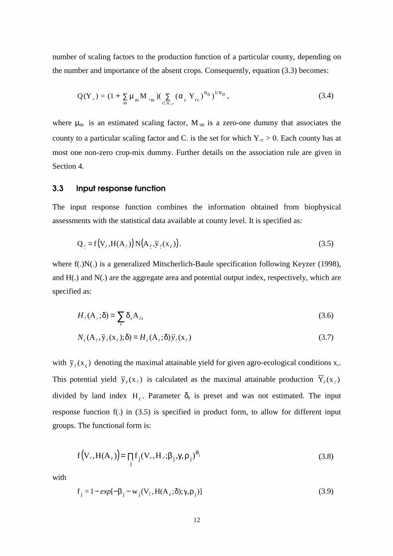
12
number of scaling factors to the production function of a particular county, depending on
the number and importance of the absent crops. Consequently, equation (3.3) becomes:
01/
Cc
0cc
mmm
))Y()(M(1=)(YQα
∈
α∑ α∑ µ+l
lll, (3.4)
where µm is an estimated scaling factor, Mlm is a zero-one dummy that associates the
county to a particular scaling factor and Cl is the set for which Y
lc > 0. Each county has at
most one non-zero crop-mix dummy. Further details on the association rule are given in
Section 4.
3.3 Input response function
The input response function combines the information obtained from biophysical
assessments with the statistical data available at county level. It is specified as:
( ) ( ))x(yAN)A(HVfQllllll
,,= . (3.5)
where f(.)N(.) is a generalized Mitscherlich-Baule specification following Keyzer (1998),
and H(.) and N(.) are the aggregate area and potential output index, respectively, which are
specified as:
∑δ=δs
sH sA);(Alll
(3.6)
)(x);(A));(xy,(Allllllll
yHN δ=δ (3.7)
with )x(yll
denoting the maximal attainable yield for given agro-ecological conditions xl.
This potential yield )x(yll
is calculated as the maximal attainable production )x(Yll
divided by land index l
H . Parameter δs is preset and was not estimated. The input
response function f(.) in (3.5) is specified in product form, to allow for different input
groups. The functional form is:
( ) ∏ ργβ= θ
jjjj
j) ,;H,V(f)(AH,Vf ,llll (3.8)
with
)],);;H(A,(Vw[1=f jjjj ργδ−β−−ll
exp (3.9)

13
where fj is the j-th component of a Mitscherlich-Baule (MB) yield function and its
exponent θj > 0 is such that 1j j =∑ θ . This parameter θj avoids the increasing returns that
would result from the standard MB-form with θj = 1. In addition, a nested structure is
assumed for inputs so as to ease the nonlinear estimation. In equations (3.8) and (3.9),
index j stands for two categories of inputs, power and nutrients. Power consists of labor
and agricultural machinery. Nutrients includes chemical and organic fertilizers. For both
categories we assume a CES form, denoted by wj.
jj
1/
jk
kkjj H
V),);;H(A,(Vw
ρ
∈
ρ
γ=ργδ ∑
l
l
ll(3.10)
with γk ≥ 0 and ρj ≤ 1 ensuring concavity of w(.). Input response function (3.5) is linear
homogeneous, globally concave and non-decreasing in (V,A), and continuously
differentiable.
The biophysical diversity across China is reflected in the potential yield )x(yll
as will be
explained in Section 4. However, cropping possibilities vary widely across China and also
within the estimated regions, ranging from single cropping to triple rice cropping. The
maximal attainable yield )x(yll
alone is not sufficient to capture this variability. To
account for these differences, cropping system zone variables z
Zl
are introduced, where
the subscript z indicates the cropping system zone. If for irrigated conditions a county is
located in cropping system zone z, the value of the related variable is 1, and 0 otherwise.
Then (3.5) becomes:
( ) ( ))x(yAN)A(HVfZQ z llllll,,= (3.11)
with
∑ζ=z
zzz ZZl
. (3.12)
The outputs in (3.4) and the potential production in (3.5) are measured in different units of
measurement. c
Yl
is given in metric tonnes of produce, while the potential is given as
cereal equivalent in metric tonnes of economic dry matter. Harmonization of the

14
dimensions is restored via the crop and county specific parameter ratio
zzmmc Z)M(1ll
ζµ+α .
3.4 Computing implicit prices for aggregation
The transformation function enters the LUC-model for China after an aggregation
procedure from county to region. Our approach is to assume “ implicit” profit
maximization, at implicit prices. These are the prices that would support the observed crop
and input allocations under profit maximization. We interpret the gap between these prices
and average market prices in the cities as processing margins, which we use in the
aggregation procedure from county to region. Clearly, this procedure needs further
empirical justification and we show in Section 5.5 that the resulting margins have a
meaningful interpretation, i.e., that despite the institutional peculiarities in China we can
indeed view the allocation decisions as being based on profit maximization, at prices
governed by institutionally determined wedges.
Assuming profit maximization subject to the separable transformation function (3.1)
ensures separability between output and input decisions. The farmer determines the crop-
mix so as to maximize the revenue corresponding to a given value of the index Q, while
choosing the level of inputs V and corresponding aggregate output Q so as to maximize
his revenue, at given prices of V and Q.
Thus, the crop-mix problem of the revenue maximizing farmer with given output index
lQ is stated as
ll
ll
l
l
Q)Q(Yts
YpCc
cc0Y c
=
∑∈
≥
.
max, (3.13)
with plc as the price of crop c in county �. The Lagrangean of this problem is:
)Q)(Q(YPYpCc
cc lllll
l
−∑ −=∈
L (3.14)
where the Lagrangean multiplier is the county level price index l
P since the function
Q(Ylc) has constant returns to scale. The first-order conditions of this problem determine
the implicit (shadow) prices of crop c∈ Cl:

15
∑ αα
=∂∂
=′
α′′
α
ccc
cc
ccc
0
0
)Y(
)Y(
Y
QP
Y
)(YQPp
l
l
l
ll
l
l
ll. (3.15)
For the base year the county level price indexl
P has been calculated from provincial and
national prices and county level production data (see annex I). In simulation runs with
endogenous crop prices cpl
the index is calculated as:
σ
∑
α∑µ+
=∈
σ1
Cc c
c
mmm
p
)M1(
1P
l
l
l
l(3.16)
with 10
0
−αα
=σ . The county specific relation between the base year price index and the
obtained under the maximizing producer assumption becomes:
)P
PP1(P)1(PP p
l
ll
llll
−+=ε+= , (3.17)
and in simulation runs the estimated price index can replace the ’observed’ index.
Finally, for the input side the restricted profit maximization problem becomes:
∑−∑−≥≥s
ssk
kk0A0V ApVp)A,V(GPsk lllllllll
,max . (3.18)
The first-order condition with respect to input k of group j gives the marginal productivity:
k
k
kk v
)v(gP
V
)A,(VGPp
l
l
l
l
ll
ll ∂∂
=∂
∂= , (3.19)
with lll
HVv kk /= and
1kk
1j
j
jj
k
k jj vwf
f1g
v
)v(g −ρρ− γ−
θ=∂
∂ll
l
l
l
l
l . (3.20)
For land-use type s the marginal productivity is:

16
∂
∂−δ=
∂
∂+
∂∂
=∂
∂=
)(v
v
v
)(v1)(v
A
)A,f(VN
A
)N(AfP
A
)A,G(VPp
s
s
s
s
ss
l
l
l
l
ll
l
ll
l
l
l
ll
l
ll
ll
g
ggP s
(3.21)
where
∑−
θ=∂∂
jj
j
jj w
f
f1
)(vg
v
v
)(vgl
l
l
l
l
l
l (3.22)
and jfl
and jwl
are the same as defined by (3.9) and (3.10).

17
4. Data: sources, adjustments, and qualifications
Despite major improvements in the quality and availability of relevant statistics for China,
various procedures had to be applied to scrutinize data, fill data gaps, and define proxy
variables, which are discussed in the present section.
4.1. Crop outputs and procurement prices
The total annual output of grain, cotton, and oilseeds is available at county level (SSB and
CDR, 1996). The published data were matched with county administrative codes as used
in the LUC Project’s database of China. Also available are output data and sown areas of
wheat, rice, maize, sorghum, millet, other starchy crops, potato and other root crops,
soybean, oilseeds, cotton, sugar beet, sugarcane, fiber crops, tobacco, tea, and fruit for
1989 but not for 1990. These data were compiled by the State Land Administration and
provided to FAO. While the year 1990 represents rather well the average conditions of
Chinese cropping agriculture during the period from 1985 to 1995, whereas the 1989-crop
was fairly poor due to weather conditions, we use data for 1990 whenever possible. As a
consequence, we had to disaggregate the data for grains in 1990 on the basis of crop-
pattern distribution available for 1989. According to Chinese statistics, the aggregate
termed grains includes wheat, rice, maize, sorghum, millet, other starchy crops, potato and
other root crops, and soybean (five kilograms of potato and other root crops are counted as
one kilogram of grain; all other commodities have a conversion factor of unity). For
sugarcane, fiber crops, tobacco, tea and fruits, the 1989 outputs had to be used.
Thus, crop outputs in 1990 were estimated as:
89
89c9090
c G
qGq ⋅= , (4.1)
where Gt is total grain output in year t and t
cq is crop-specific output measured in grain
equivalent. For vegetables, only estimates of sown areas at county level for 1989 were
available, and no output data for any year. The national average yield of 20.9 tons per
hectare in 1989 was used (Xie and Jia, 1994, p. 103) to calculate vegetable output at
county level.
Procurement prices at both provincial and national levels for wheat, rice, maize, sorghum,
millet, soybean, oilseeds, cotton, sugarcane, fiber crops, tobacco, tea, and fruit were

18
extracted from Yearbook of Price Statistics of China 1992 (SSB, 1992b, pp. 302-365). The
procurement price for a crop is a quantity-share-weighted mean of quota prices, negotiated
prices, and free-market prices. The procurement of commodities is done not only by
government agencies, but also enterprises, social organizations, and trade companies.
There is no price data for Hainan Province in this Yearbook. Prices in Guangdong were
used as proxies for Hainan in view of the fact that Hainan Province had been a prefecture
of Guangdong until 1988. No price data are available for the aggregate of other starchy
crops. The price of maize is used as a proxy in each province following the information in
the national price data for China listed in the FAO-AGROSTAT database. Again with
reference to FAO-AGROSTAT, one third of wheat price is used as a proxy for the price of
potato and other root crops in each province.
Prices of vegetables were compiled from Nationwide Data on Costs and Revenues of
Agricultural Products 1991 (Eight Ministries and Bureaus, 1991). The prices listed in this
publication are free-market selling prices of major vegetables shown for selected major
cities (typically, provincial capital city) in most of the provinces. Representative
vegetables for each province were selected and the representative price for the vegetable
category is the arithmetic mean of the various prices.
With the steps described in the previous paragraphs, price data could be obtained for all
major crops of each province. However, the price information for some minor crops was
still missing, and these are actually the main crops in some counties. To fill these gaps, a
corresponding price was used from one of the neighboring provinces with similar
production conditions. When no such province was available, the national average price
was used as a proxy.
In the compilation of the initial output index Q, the provincial prices were applied directly
to the county level, ignoring all price differences across counties within each province.
4.2 Non-land and land inputs
Data on non-land inputs used in the broad agricultural sector at county level are available
in the LUC project for various years between 1985 to 1994. They include agricultural
labor force, total power of agricultural machinery, total number of large animals, and
chemical fertilizer applied. In the following we will only discuss the 1990 data since these
were used in estimation. A data problem arises from the fact that in Chinese statistics,

19
broad agriculture consists of farming, forestry, animal husbandry, fishery, and sideline
production. We attribute non-land inputs to the crop sector based on the share of crop
agriculture in broad agriculture. The total output value of broad agriculture is available at
county level. Availability of crop output enables us to calculate the total output value of
cropping agriculture for each county by straight aggregation over crops valued at
provincial prices. The resulting shares are applied to agricultural labor force and power of
agricultural machinery8.
Two remarks are in order. First, the approach is questionable for counties where the share
of cropping agriculture is minor or where agricultural workers or machinery are in fact
used for non-agricultural activities. In some (sub-)urban counties the number of
agricultural workers per hectare of agricultural land is extremely high (more than 10).
Machine power per hectare is likewise biased due to the fact that transport vehicles and
other processing machineries are included in the statistics. Nonetheless these counties
were initially included in the estimations. After the first round some of the counties biased
the estimation substantially and these observations were dropped. Secondly, prices are at
provincial level and, consequently, the variability at county level depends on quantities
alone.
Whereas "chemical fertilizer applied" can safely be attributed to crop farming rather than
to forests or pastures, organic fertilizer data can only be derived by imputation. We follow
the approach in Wen (1993, Tables 4 and 5) and assume that (i) one person produces 0.5
tons of night soil per year on average; the utilization rates of night soil in the rural and
urban areas are 0.8 and 0.4, respectively, in 1990; the nutrient content rate of night soil is
0.011, i.e., 1.1 percent; (ii) a large animal produces 7.7 tons of manure per year on
average; the utilization rate is 0.8; the nutrient content rate is 0.0102; and (iii) hog manure
is assumed to be 2 tons per animal per year, with a utilization rate 0.8, and a nutrient
content rate of 0.014. No systematic data is available on other sources of organic fertilizer
such as green fertilizer, oil cake, compost, and mud and pond manure. The resulting
estimate of the national total at 17.5 million tons of organic fertilizer supply is 6 million
tons lower than Wen’s 1989 figure, but 7 million tons higher than the corresponding 1991
figure given by the Agricultural Academy of China (1995, p. 95). In some counties, where
8 We used the total number of large animals as a proxy for draught animals. However, due to the poorperformance of this proxy in all estimations, we finally had to drop it from the estimation.

20
animal husbandry plays a key role, the manure of large animals may dominate in total
organic fertilizer, and animal manure often is used as fuel rather than as plant nutrient.
Hence, to avoid unrealistically high estimates of organic fertilizer application in these
counties, we impose a ceiling of 120 tons raw organic fertilizer manageable per worker per
year (Wiemer, 1994), which is equivalent to about 1.2 tons of nutrient content.
For farmland, we use the county level data on total cultivated land areas and irrigated land
compiled by China’s State Land Administration (SLA). The national total of cultivated
land areas obtained by summation over counties is some 135 million hectares, which is
about 40 million hectares higher than the corresponding national figure published in the
Statistical Yearbook of China (SSB, 1991, p. 314), but is quite consistent with the figure
recently compiled by the SLA, based on a detailed land survey9 (see Fischer et al., 1998).
In addition to statistical data, the LUC project database includes several digital coverages
for China, including climate, land use, vegetation, altitude and soils. These were compiled,
re-organized and edited jointly with the Chinese collaborators in the LUC project to
provide a basis for biophysical assessments of surface hydrology, vegetation distribution,
and for estimating potential yields of major crops10. Although these maps provide useful
spatial information for land-use research, their scale is insufficient to derive accurate
overlays of the actual farmland in 1990 with soil and terrain resources for differentiating
land quality types among actual farmland. Hence, the land quality types (index s) applied
at county level currently only distinguish irrigated and rain-fed land.
In actual farming practice, the distinction between irrigated and rain-fed land is not as
strict as suggested by the statistical figures. In some areas, when rainfall comes in time for
cropping and in adequate amounts, irrigation is not necessary and the differentiation
between irrigated and rain-fed land becomes unimportant. And conversely, when the water
shortage is severe, irrigation may be impossible despite existing irrigation facilities.
9 Personal communications with Chinese officials suggest that the farmland data compiled by SLA based ondetailed surveys will eventually replace the unrealistic estimates published in the Statistical Yearbook ofChina. Except where specifically mentioned, the data in this sub-section are derived from variouspublications of China’s State Statistical Bureau.
10 For detailed documentation and references regarding the compilation and editing of these land use andsoil maps, see http://www.iiasa.ac.at/Research/LUC/
21
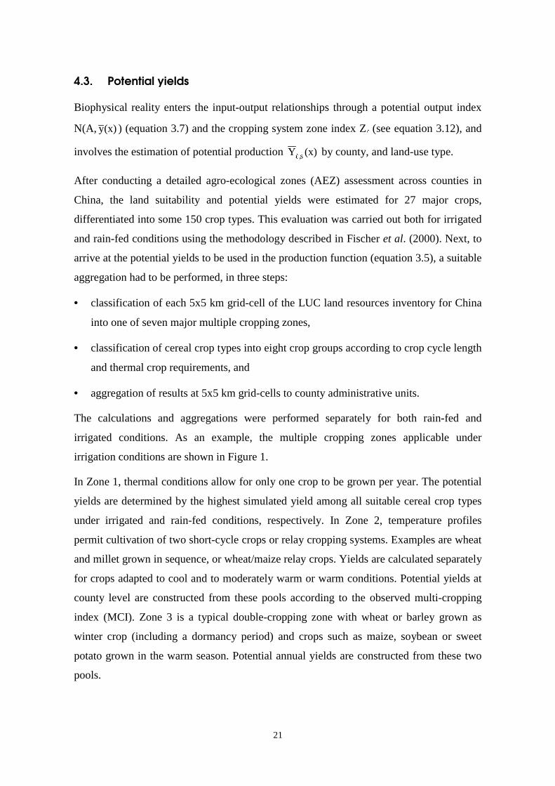
4.3. Potential yields
Biophysical reality enters the input-output relationships through a potential output index
N(A, (x)y ) (equation 3.7) and the cropping system zone index Zl (see equation 3.12), and
involves the estimation of potential production (x)Y s,l by county, and land-use type.
After conducting a detailed agro-ecological zones (AEZ) assessment across counties in
China, the land suitability and potential yields were estimated for 27 major crops,
differentiated into some 150 crop types. This evaluation was carried out both for irrigated
and rain-fed conditions using the methodology described in Fischer et al. (2000). Next, to
arrive at the potential yields to be used in the production function (equation 3.5), a suitable
aggregation had to be performed, in three steps:
• classification of each 5x5 km grid-cell of the LUC land resources inventory for China
into one of seven major multiple cropping zones,
• classification of cereal crop types into eight crop groups according to crop cycle length
and thermal crop requirements, and
• aggregation of results at 5x5 km grid-cells to county administrative units.
The calculations and aggregations were performed separately for both rain-fed and
irrigated conditions. As an example, the multiple cropping zones applicable under
irrigation conditions are shown in Figure 1.
In Zone 1, thermal conditions allow for only one crop to be grown per year. The potential
yields are determined by the highest simulated yield among all suitable cereal crop types
under irrigated and rain-fed conditions, respectively. In Zone 2, temperature profiles
permit cultivation of two short-cycle crops or relay cropping systems. Examples are wheat
and millet grown in sequence, or wheat/maize relay crops. Yields are calculated separately
for crops adapted to cool and to moderately warm or warm conditions. Potential yields at
county level are constructed from these pools according to the observed multi-cropping
index (MCI). Zone 3 is a typical double-cropping zone with wheat or barley grown as
winter crop (including a dormancy period) and crops such as maize, soybean or sweet
potato grown in the warm season. Potential annual yields are constructed from these two
pools.

22
Figure 1. Multiple cropping zones under irrigated conditions.
Zone 4 has double cropping similar to the previous zone, except that the main summer
crop such as rice or cotton demands more heat. Zone 5 is generally found south of the
Yangtse, and permits limited triple cropping consisting of two rice crops and, for instance,
green manure. The annual temperature profile is usually insufficient for growing three full
crops. When the observed MCI does not exceed 2.0, the combination of the best suitable
crops during the cooler and warmer seasons of the year defines the potential annual yield.
The more the observed MCI exceeds 2.0, the less applicable are crop types with long
growth cycles because of the time limitations. When the MCI approaches 3.0 only crop
types requiring 120 days or less are considered when calculating annual output. Zone 6
occurs in southern China and allows three sequential crops to be grown. A typical example
is the cropping system with one crop of winter wheat and two rice crops grown in spring
to autumn. In this case, only short cycle crops can be considered.

23
Table 1. Number of counties per cropping system zone by region
Region
North North-East East Central South South-WestNorth-West/
Plateau
Single cropping 94 138 62 200
Limited double 111 21 10 64 48
Double cropping 287 73 14 102 22
Double with rice 115 171 18 90
Double rice 41 62 39 66
Triple cropping 116
Triple rice 78
Total 492 159 229 257 251 384 270
Figure 2. Annual potential production (tons/ha), weighted average of irrigation andrain-fed potentials.
Finally, Zone 7 delineates the most southern part of China where tropical conditions
prevail, and allows three crops to grow that are well adapted to warm conditions, e.g., rice.
In our calculation, this condition is satisfied when the growing season is year-round and
24
annual accumulated temperature (above 10ºC) exceeds 7000 degree-days. Only crop types
requiring less than 120 days until harvest are considered when the MCI exceeds 3.0.
Table 1 shows the number of counties in each cropping system zone under irrigated
conditions to be used in the estimation. If there were only very few counties in a cropping
system zone of a particular region the observations were added to the adjacent zone.
Figure 2 summarizes the results of the biophysical assessment weighted by actual shares
of irrigated and rain-fed cultivated land in each county.
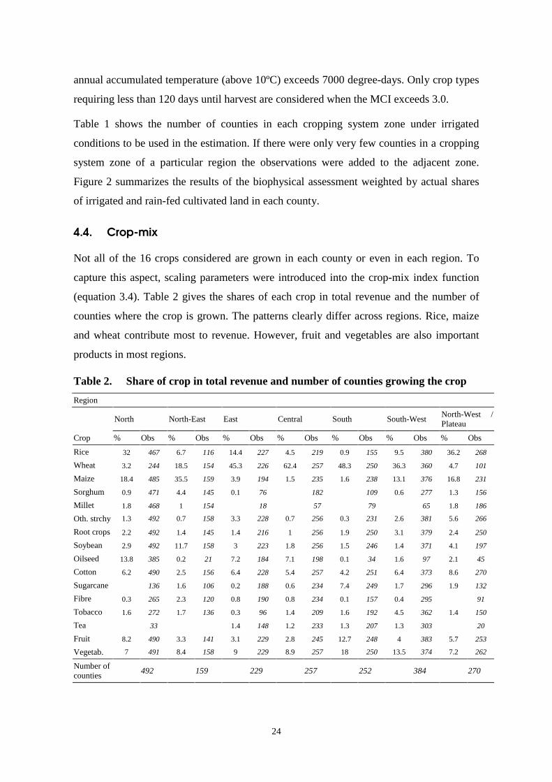
4.4. Crop-mix
Not all of the 16 crops considered are grown in each county or even in each region. To
capture this aspect, scaling parameters were introduced into the crop-mix index function
(equation 3.4). Table 2 gives the shares of each crop in total revenue and the number of
counties where the crop is grown. The patterns clearly differ across regions. Rice, maize
and wheat contribute most to revenue. However, fruit and vegetables are also important
products in most regions.
Table 2. Share of crop in total revenue and number of counties growing the crop
Region
North North-East East Central South South-WestNorth-West /Plateau
Crop % Obs % Obs % Obs % Obs % Obs % Obs % Obs
Rice 32 467 6.7 116 14.4 227 4.5 219 0.9 155 9.5 380 36.2 268
Wheat 3.2 244 18.5 154 45.3 226 62.4 257 48.3 250 36.3 360 4.7 101
Maize 18.4 485 35.5 159 3.9 194 1.5 235 1.6 238 13.1 376 16.8 231
Sorghum 0.9 471 4.4 145 0.1 76 182 109 0.6 277 1.3 156
Millet 1.8 468 1 154 18 57 79 65 1.8 186
Oth. strchy 1.3 492 0.7 158 3.3 228 0.7 256 0.3 231 2.6 381 5.6 266
Root crops 2.2 492 1.4 145 1.4 216 1 256 1.9 250 3.1 379 2.4 250
Soybean 2.9 492 11.7 158 3 223 1.8 256 1.5 246 1.4 371 4.1 197
Oilseed 13.8 385 0.2 21 7.2 184 7.1 198 0.1 34 1.6 97 2.1 45
Cotton 6.2 490 2.5 156 6.4 228 5.4 257 4.2 251 6.4 373 8.6 270
Sugarcane 136 1.6 106 0.2 188 0.6 234 7.4 249 1.7 296 1.9 132
Fibre 0.3 265 2.3 120 0.8 190 0.8 234 0.1 157 0.4 295 91
Tobacco 1.6 272 1.7 136 0.3 96 1.4 209 1.6 192 4.5 362 1.4 150
Tea 33 1.4 148 1.2 233 1.3 207 1.3 303 20
Fruit 8.2 490 3.3 141 3.1 229 2.8 245 12.7 248 4 383 5.7 253
Vegetab. 7 491 8.4 158 9 229 8.9 257 18 250 13.5 374 7.2 262
Number ofcounties
492 159 229 257 252 384 270

25
Table 2 does not capture the broad variation of over 400 crop combinations, which enter
the model through the crop (-mix) variables Mm. Their definition is listed in Table 3.
Guiding principles in the definition of crop-mix variables were: (i) not to exceed a total of
4 crop-mix parameters, and (ii) to give missing major crops priority over the less
important ones. Each county has at most one nonzero crop-mix dummy. Table 4 presents
the results of these crop-mix definitions.
Table 3. Definition of crop-mix variables Mm (entries are crops missing)
Mix 1 Mix 2 Mix 3 Mix 4 No mix
North Wheat Maize/ Cotton/ Fruit ≥ 3 smaller crops - All other cases
North-East Maize/ Rice/Soybean/ Vegetables
Wheat ≥3 smaller crops - All other cases
East Rice or Wheat ≥ 5 smaller crops - - All other cases
Central Rice/ Vegetables/Cotton
≥ 3 smaller crops - - All other cases
South Rice/ Vegetables/Fruit/ Sugarcane
≥ 3 smaller crops - - All other cases
South-West 1 of Rice/Vegetables/ Maize/
Wheat
2 or 3 of Wheat/Rice/ Vegetables/
Maize
- - All other cases
North-West /Plateau
1 of Wheat/ Maize/Fruit/ Vegetables
2 or 3 of Wheat/Maize/ Fruit/Vegetables
4 or 5 smaller crops ≥ 6 smallercrops
All other cases
Table 4. County number corresponding to the crop-mix variables by region
Region
North North-East East Central South South-WestNorth-West /
Plateau
None 130 88 200 159 123 163 87
Mix 1 25 7 5 59 7 14 36
Mix 2 87 42 25 39 121 13 8
Mix 3 250 22 194 101
Mix 4 38
Total 492 159 229 257 251 384 270
4.5. Data checking
Multiple checks were conducted in order to improve data reliability and consistency. This
was done on the basis of checking various relative indicators such as the irrigation ratio,
land per laborer, land per capita, output per sown hectare, and each non-land input per
hectare and per laborer. Occasionally, errors in the original publications could be corrected
by comparison of different data sources. In some cases missing or dubious data could be

26
corrected by reference to data for other years. When data was missing or appeared to be
highly implausible but could not be corrected by using other sources, the respective county
was dropped from the estimation.
Table 5. Observations per region
Regions
North North-East East Central South South-WestNorth-West /
PlateauTotal
All counties 510 184 244 275 272 402 491 2378
Missing data 13 25 15 18 21 18 212 322
Outliers(Labor/Machinery) 5 0 0 0 0 0 9 14
For estimation 492 159 229 257 251 384 270 2042
Eventually, of the 2378 administrative units contained in the LUC database in total, 2042
counties could be retained in the study, i.e., data were complete and were judged
sufficiently reliable to be used for the output side as well as the input side of the
estimation. Table 5 gives an account by region. Incomplete county level records
eliminated 322 counties, and outliers mainly for labor and machinery figures eliminated
another 14 (see also Section 4.2 above). These outliers were concentrated in the North,
Plateau and North-East regions. Only 20 counties on the Plateau located in the Qinghai
province qualified for inclusion in the estimation. Xizang (Tibet) had no acceptable data
records at all. Consequently, it was decided to pool Qinghai with the North-West region
based on the similarity of cropping zone pattern.

27
5. Results from estimation
Parameters of the model, which was described in Section 3, were estimated by Nonlinear
Least Squares (NLS) for each region separately, except that the North-West region and
Plateau (i.e., a few counties in Qinghai Province) were treated jointly because the number
of valid observations (some 20) was too low for the Plateau region to be estimated
separately. The presentation of results proceeds as follows. In Section 5.1, we check
whether the error term meets the statistical requirements, which permit to consider NLS as
a maximum likelihood estimator. Next, we discuss the estimation results of the input
response function G (Section 5.2). Coefficient values of the output index Q are reported in
Section 5.3. Finally, in Section 5.4 we present and discuss the spatial distribution of
calculated implicit (shadow) prices and in Section 5.5 of the marginal productivity of input
factors.
5.1 Analysis of error term
To test whether Nonlinear Least Squares amounts to maximum likelihood estimation, we
check normality, homoscedasticity and independence of the error term. We apply two
tests, one parametric and one non-parametric. First, we use the common Shapiro-Wilk test
(Shapiro and Wilk, 1965) to check whether for the sample as a whole the errors are a
random sample from the normal distribution. Secondly, we check whether errors might be
spatially correlated, albeit locally. This is done by applying a spatial non-parametric
(kernel density) regression (Bierens, 1987; Keyzer and Sonneveld, 1997) regressing the
error term on longitude and latitude of the counties. For each county, the estimated value
is calculated, the derivative with respect to longitude and latitude and the estimated
probability of wrong sign for that derivative is calculated. Lack of spatial correlation finds
expression in frequently changing signs of the derivatives and a high average probability
of wrong sign of the derivatives.
Table 6 presents the Shapiro-Wilk statistic. The normality test is passed at 5 percent level
for all regions. The table also shows results from kernel density regression and indicates
that no spatial dependency could be detected anywhere. On average, the probability of a
wrong sign of the derivative in either direction is close enough to 0.5, implying that the
error term could vary in any direction. Therefore, there is no need to correct for spatial

28
correlation of errors in the regression and that homoscedasticity and independence can be
assumed.
Table 6. Tests on the error termRegion
Coefficient North North-East East Central South South-WestNorth-West /Plateau
Shapiro-Wilk’s W .989 .977 .986 .982 .980 .988 .983
Probability < W .876 .231 .726 .416 .234 .820 .453
Spatial dependency using the mollifier method
Probability of wrong sign of derivative:
Longitude .454 .443 .454 .461 .458 .465 .446
Latitude .441 .418 .455 .457 .452 .448 .423
We conclude that the model can be estimated by least squares. Appendix I describes an
iterative numerical procedure to perform this estimation.
5.2 Input response
Next, we report on the coefficient values and their likelihood ratios and on the elasticities
of the input response equations, recalling that these were actually estimated
simultaneously with the output mix equations. The likelihood ratio is used to check the
robustness of the coefficients.
Let us briefly recapitulate its main principles first (see Gallant, 1987; Davidson and
MacKinnon, 1993). We denote model parameters by 21 ζζ , . Under our null hypothesis H0:
11 ζ=ζ and 2ζ unrestricted while under the alternative H1: both 1ζ and 2ζ are
unrestricted. With maximum likelihood estimation, the significance level of an estimated
parameter 1ζ̂ can be determined by an F-test: j
mn
S
S −⋅
−=− 1
)2ˆ,1
ˆ(
)2~
,1(m)nF(j,
ζζζζ
, where
n, m and j are the number of observations, parameters and restrictions, respectively;
)(S 21 ζζ ˆ,ˆ is the minimum residual sum of squares corresponding to maximization of the
unrestricted likelihood function, and )~
,( 21 ζζS is the residual sum of squares for given
reference value 1ζ and free 2
~ζ , corresponding to maximization of the restricted likelihood
function. Critical value for the region with smallest sample size (i.e., the North-East
region) F(1,159) at 0.95 is 3.83.

29
As a reference value we use 50 percent11 of the original estimate1ζ̂ , as opposed to the
usual reference value zero because the function form is given and all variables have to
enter the welfare model eventually. Hence, we need to assess the robustness of the
estimated parameter value, rather than deciding whether the variable should be included at
all.
Coefficients
Table 7 presents the estimated coefficients of the input response function index G, their
corresponding likelihood ratios (LR, in italics), and the number of observations in each
region. Clearly, for parameters with zero value no likelihood ratio can be calculated. Since
Σjθj = 1 no LR for θNutrient is estimated. As the parameter δRainfed is by definition equal to
unity it has no LR value.
Table 7. Estimated coefficients for the input response function
Region
Coefficient North North-East East Central South South-WestNorth-West /Plateau
ζsingle cropping 0.939 182.131 - - - 3.050 40.205
33.8 136.6 258.0 129.3
ζLimited double 0.892 169.202 - 5.150 - 2.217 32.751
41.8 75.0 92.5 208.2 151.3
ζDouble cropping 0.841 - 5.983 4.353 - 2.111 33.862
43.6 711.4 159.9 275.5 154.9
ζDouble with rice - - 5.768 3.502 2.806 1.891 -
793.6 595.0 111.8 32.8
ζDouble rice - - 5.169 2.887 2.553 1.742 -
636.0 2077.7 178.8 62.9
ζTriple cropping - - - - 2.365 - -
30.5
ζTriple rice - - - - 2.595 - -
78.7
11 The alternative values against which the estimated values are tested read: θPower = .5, ζz = 1, µm = 0,ρPower = −1.5, ρNutrient = .7 or 1. and α0 = 2. For δIrrigated=1, the ratio between the potential yield onirrigated land to the potential yield on rain-fed land is used as the alternative, in the other cases ifδIrrigated=1 is the hypothesis. Leading to the values δIrrigated = 1.00, 1.00, 1.05, 1.04, 1.03, 1.16 and 1.00,respectively, for the various regions.

30
Table 7. Estimated coefficients for the input response function (cont.)
Region
Coefficient North North-East East Central South South-WestNorth-West /Plateau
θPower 0.320 0.700* 0.430 0.365 0.341 0.300* 0.555
376.6 772.9 4.8 115.4 160.2 210.7 22.7
θNutrient 0.680 0.300 0.570 0.635 0.659 0.700 0.445
βPower 0.000 0.000 0.013 0.001 0.005 0.006 0.001
20.8 68.7 122.7 33.9 16.8
βNutrient 0.000 0.031 0.005 0.000 0.000 0.013 0.003
2.8 96.6 15.4 10.6
ρPower -0.250* -0.250* -0.250* -0.250* -0.250* -1.630 -1.265
43.4 126.1 15.5 20.4 24.1 74.6 48.9
ρNutrient 0.700* 0.700* 1.000* 1.000* 1.000* 1.000* 0.700*
30.8 17773.5 16.8 3552.1 243.1 255.3 3.2
γLabor 0.161 2.062 0.464 0.389 0.291 3.010 7.856
30.0 14.5 15.7 50.2 40.9 22.5 16.6
γMachine 0.807 2.141 1.024 1.779 1.457 3.179 23.589
446.5 12.1 153.5 2264.7 817.3 34.9 22.6
γChemicals 3.235 0.337 0.160 1.578 0.728 0.934 0.120
38.0 10.8 549.5 826.3 174.4 12.8 12.5
γOrganic 1.481 0.025 0.135 0.770 0.623 0.387 0.029
37.8 11.2 97.3 75.5 28.3 37.8 13.8
δIrrigated¹ 2.110 1.590 1.000 1.000 1.000 1.000 2.210
35.5 4.9 117.2 54.4 28.7 30.6 22.2
δRainfed¹ 1.000 1.000 1.000 1.000 1.000 1.000 1.000
Observations 492 159 229 257 173 384 270
* parameter at bound, ¹ preset value
As described in Section 3.3, the area index H(A) is preset before estimation. The
parameter δIrrigated converts irrigated land into rain-fed equivalent. It is chosen on the
interval between unity and the ratio of potential yield on irrigated land to potential yield on
rain-fed land and its significance was assessed (see previous footnote). The estimation
results for the North-East region are generally slightly deviant on the input side. The
quality of the input data and potential production in North-East is probably causing this
result. Except for βNutrient in North-East all parameters are significant at 95 per cent level.
Not surprisingly, the input specific parameters γ show a large range of variability across
regions, justifying estimation by region as opposed to a pooled estimation for China as a

31
whole. For the Northern regions, i.e. North-West/Plateau, North and North-East, fertilizer
substitution is at the lower bound and relatively inelastic (elasticity of substitution εNutrient
= 3.33). Generally, the constants β of the input groups are small or zero. The upper bound
for ρPower of -.25 is in effect for five regions. The substitution elasticities for the power-
related inputs range from 0.38 in South-West to 0.80 in most other regions. .
Elasticities and marginal values
As a further description of the results from estimation, we present in Table 8 the output
elasticities by input category, evaluated at the regional mean (see Appendix II for a
specification of the analytical form of elasticities). Since the input response function G is
linear homogeneous of degree one in (V, A), the elasticities of the inputs add up to unity.
Table 8. Output elasticities of land and non-land inputs at the regional mean
Region
Input North North-East East Central South South-WestNorth-West /
Plateau
Labor 0.052 0.172 0.095 0.054 0.036 0.028 0.100Machinery 0.248 0.160 0.216 0.279 0.202 0.211 0.331
Power 0.300 0.332 0.311 0.333 0.238 0.239 0.431Chemical fertilizer 0.309 0.122 0.392 0.344 0.376 0.398 0.209Organic fertilizer 0.084 0.005 0.121 0.102 0.184 0.192 0.042
Nutrient 0.393 0.127 0.513 0.446 0.560 0.590 0.251Irrigated area 0.215 0.140 0.131 0.165 0.127 0.063 0.138Rain-fed area 0.092 0.401 0.045 0.056 0.075 0.108 0.180
Land 0.307 0.541 0.176 0.221 0.202 0.171 0.318Elasticity of land-index H if change is attributed to:
Irrigated area 0.414 0.779 0.185 0.221 0.203 0.171 0.544Rain-fed area 0.196 0.490 0.185 0.221 0.203 0.171 0.246
The results suggest a differentiation into three zones. First, the Southeast part of China,
i.e., regions East, Central, South and to some extend South-West. They show a great
similarity in elasticities for most inputs and input groups (Power, Nutrient and Land). The
elasticity is highest for chemical fertilizer, followed by machinery and irrigated land,
while labor has a small contribution to the output index. Second, we identify the regions
North and North-West/Plateau where the similarity between the elasticities manifests
mainly in their pattern with respect to the non-land inputs and not so much in their levels.

32
The levels of elasticities in North are comparable to the first zone. Finally, in the
remaining region, North-East, the picture is different with the highest elasticity for labor.
The elasticities of land-use types might convey the wrong impression that investment in
irrigation in North-East, South-West and North-West/Plateau is not profitable. In fact the
lower elasticities for irrigated land in some region merely reflects the lower area under
irrigation (see Appendix II.2). For example, in North-East rain-fed agriculture is the
dominant land-use type (78 percent) and δIrrigated is 1.59 resulting in a ratio of the rain-fed
over irrigated land of about 2.9. To assess the relative productivity of investment into
irrigated and non-irrigated, a common area basis is needed. The two lines at the bottom of
Table 8 measure the percentage increase in output if the land basis expands by one per
cent of irrigated and non-irrigated land, respectively. Since δIrrigated exceeds δRainfed,
irrigation appears to be more productive.
Figure 3 and 4 map the county level elasticities for labor and machinery and seems to
confirm the spatial pattern of the regional averages. The maps are computed on the basis
of kernel density regression as in Keyzer and Sonneveld (1997). The histogram on the left
Figure 3. Elasticity for labor

33
of each panel shows the percentage shares of the colored areas. A combined mask of
estimated counties and agricultural areas as given by Figure 1 is applied.
As a further characterization of the differences across regions, we calculate the marginal
values (see Table 9). These reflect the variability of implicit wages, rental cost of
machinery, and price of chemical and organic fertilizers.
The marginal value of labor is high in the Northern regions and, as could be expected, low
in densely populated areas of the Central and South regions where marginal returns to land
are relatively high for both irrigated and rain-fed land. Despite its dense population, the
East region reflects, with the relatively high marginal value of labor, the attractiveness of
the more industrialized area.
Figure 4. Elasticity for machinery
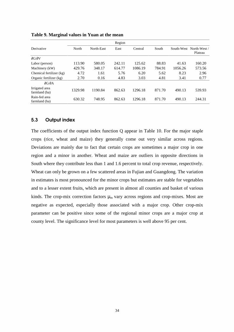
34
Table 9. Marginal values in Yuan at the mean
Region
Derivative North North-East East Central South South-West North-West /Plateau
∂G/∂VLabor (person) 113.90 580.05 242.11 125.62 88.83 41.63 160.20Machinery (kW) 429.76 348.17 614.77 1086.19 784.91 1056.26 573.56Chemical fertilizer (kg) 4.72 1.61 5.76 6.20 5.62 8.23 2.96Organic fertilizer (kg) 2.70 0.16 4.83 3.03 4.81 3.41 0.77
∂G/∂AIrrigated areafarmland (ha)
1329.98 1190.84 862.63 1296.18 871.70 490.13 539.93
Rain-fed areafarmland (ha)
630.32 748.95 862.63 1296.18 871.70 490.13 244.31
5.3 Output index
The coefficients of the output index function Q appear in Table 10. For the major staple
crops (rice, wheat and maize) they generally come out very similar across regions.
Deviations are mainly due to fact that certain crops are sometimes a major crop in one
region and a minor in another. Wheat and maize are outliers in opposite directions in
South where they contribute less than 1 and 1.6 percent to total crop revenue, respectively.
Wheat can only be grown on a few scattered areas in Fujian and Guangdong. The variation
in estimates is most pronounced for the minor crops but estimates are stable for vegetables
and to a lesser extent fruits, which are present in almost all counties and basket of various
kinds. The crop-mix correction factors µm vary across regions and crop-mixes. Most are
negative as expected, especially those associated with a major crop. Other crop-mix
parameter can be positive since some of the regional minor crops are a major crop at
county level. The significance level for most parameters is well above 95 per cent.

35
Table 10. Estimated coefficients for the output functionRegion
CoefficientNorth North-East East Central South South-WestNorth-West /
Plateau
α01
1.500 1.500 1.500 1.500 1.500 1.500 1.500
46.6 25.4 29.9 35.6 35.1 74.4 42.7
αRice 0.780 0.727 0.892 0.752 0.712 0.839 0.890
36.4 1.3 199.8 281.8 111.4 93.2 18.3
αWheat 1.171 0.881 1.099 1.374 5.425 1.035 1.024
163.7 5.0 21.0 32.3 33.1 28.5 17.0
αMaize 1.433 0.668 3.863 10.922 13.532 0.030* 0.030*
38.4 11.1 14.5 23.5 23.0 31.9 16.5
αSorghum 2.095 0.168 0.030* 0.030* 49.332 0.030* 0.793
43.7 5.0 14.5 17.3 20.5 30.3 16.9
αMillet 0.720 0.586 0.934 0.806 2.346 1.205 0.672
48.7 9.4 16.0 17.7 39.6 68.5 19.7
αOther starchy 0.944 3.588 0.714 2.592 0.030* 0.592 0.159
30.9 6.9 14.2 16.5 18.8 33.3 17.6
αRoot crops 0.383 0.030* 0.534 0.724 0.030* 0.841 0.95930.2 5.9 14.7 16.5 19.9 33.1 16.2
αSoybean 2.624 1.231 3.467 6.385 0.030* 0.030* 0.030*
33.7 3.9 15.3 17.8 20.1 30.0 16.9
αOilseed 1.324 0.503 3.300 4.417 7.972 2.361 0.526
28.2 5.4 17.7 23.9 31.3 29.1 17.0
αCotton 6.796 35.730 10.066 9.360 6.079 18.836 11.477
46.8 5.5 17.6 22.0 22.7 33.3 22.0
αSugarcane 1.043 0.030* 0.536 0.342 0.201 0.212 0.563
35.9 5.0 14.7 15.8 24.1 49.6 20.7
αFiber 4.802 0.030* 2.889 2.577 13.924 11.246 39.267
34.6 5.0 13.7 15.3 21.8 24.2 16.3
αTobacco 3.203 8.088 0.030* 7.062 6.844 4.713 1.391
31.5 7.3 14.3 32.8 23.4 45.5 18.3
αTea 31.912 - 10.469 12.199 17.698 11.082 0.030*
32.8 17.7 17.0 24.6 31.7 17.2
αFruit 1.674 1.241 1.427 2.504 1.901 2.206 1.885
30.1 7.3 15.3 24.1 21.5 28.9 15.3
αVegetables 0.346 0.267 0.364 0.484 0.347 0.461 0.335
42.1 7.9 26.9 29.9 18.9 64.2 19.4
µMix 1 -0.182 -0.182 -0.076 -0.014 0.121 -0.215 -0.376
41.6 7.7 12.5 14.1 20.8 35.1 34.4
µMix 2 -0.083 0.203 -0.119 -0.043 0.054 -0.031 -0.022
41.8 10.9 29.8 20.8 24.0 30.7 16.6
µMix 3 -0.014 0.021 - - - -0.034 -0.043
32.3 5.0 35.7 21.3
µMix 4 - - - - - - 0.019
17.6
* parameter at bound, ¹ preset value

36
5.4 Implicit prices
We are now ready to calculate implicit prices along the lines set out in Section 3.6, and
compare these with the consumer prices in nearby urban centers. The difference between
both measures an implicit trade and transportation margin. Clearly, this margin should
increase with the distance to the main consuming areas. We show results for rice and
wheat, the major staples, by means of a price map computed through kernel density
regression.
Figure 5 displays the implicit price of rice for the main rice producing provinces. Figure 6
shows the population density in 100 persons per km². It appears that the farm gate price of
rice is in general higher in areas with a high population density. This holds especially for
the relatively urbanized areas in the Southern provinces Guandong, Guanxi and Hainan.
Also the Red Basin area in Sichuan and the Dongbei Pingyuan Plains stretching from
South to North in the three North-Eastern provinces exhibit rising prices closer to
consuming areas. Thus, the figures indicate that our (purely quantity based) estimation
results in a positive trade and transportation margin.
Figure 5. Shadow price of rice (Yuan/kg)

37
The implicit prices of the two other major crops, wheat and maize, for the relevant
producing areas are shown in Figures 7 and 8, respectively. The picture also shows prices
rising as one comes nearer to densely populated areas. Wheat has an outlier in the South
region, resulting in high farm gate price. Note that there is no wheat in the plains of the
North-East where the conditions are more favorable for maize, which is grown on more
than 50 percent of the area.
Figure 6. Population density (persons/km2)

38
Figure 7. Shadow price of wheat (Yuan/kg)
Figure 8. Shadow price of maize (Yuan/kg)
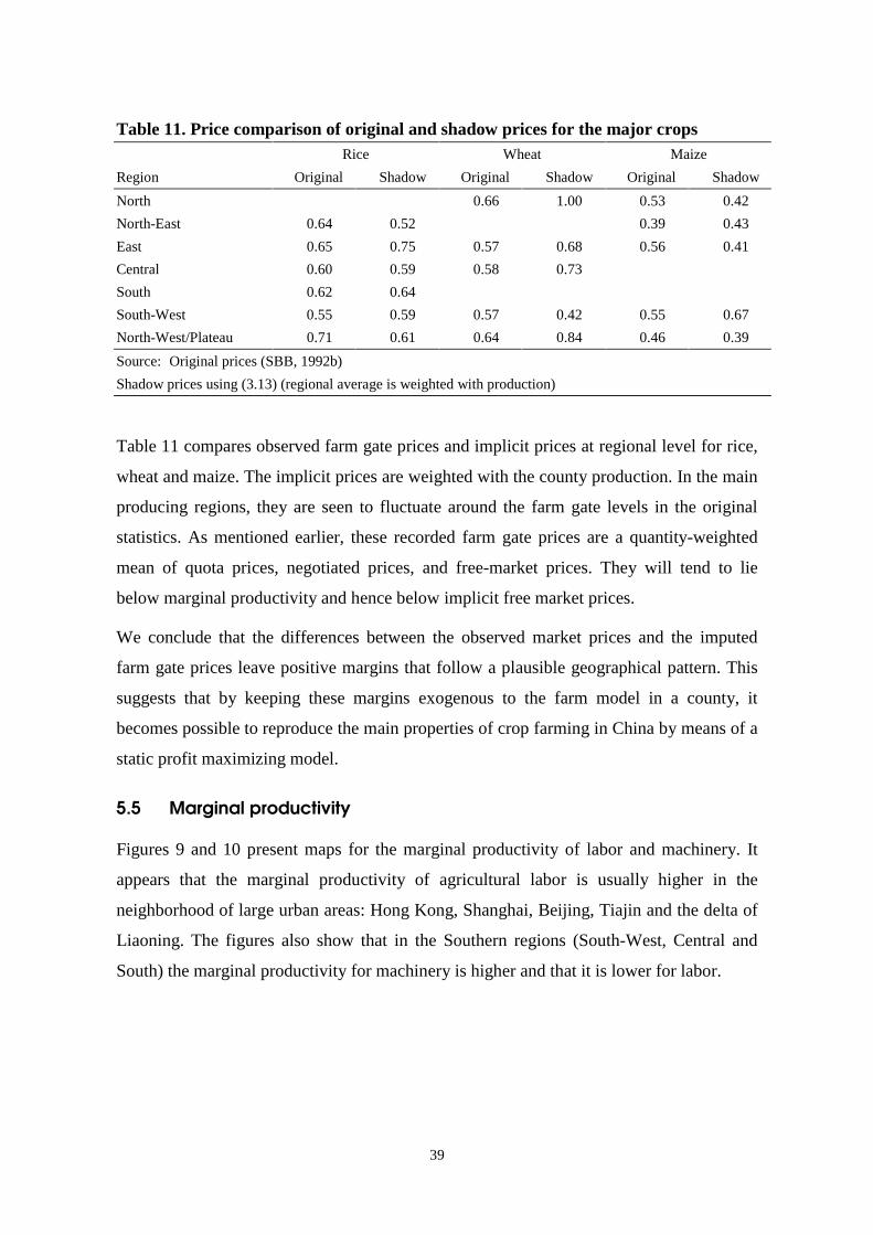
39
Table 11. Price comparison of original and shadow prices for the major cropsRice Wheat Maize
Region Original Shadow Original Shadow Original Shadow
North 0.66 1.00 0.53 0.42
North-East 0.64 0.52 0.39 0.43
East 0.65 0.75 0.57 0.68 0.56 0.41
Central 0.60 0.59 0.58 0.73
South 0.62 0.64
South-West 0.55 0.59 0.57 0.42 0.55 0.67
North-West/Plateau 0.71 0.61 0.64 0.84 0.46 0.39
Source: Original prices (SBB, 1992b)
Shadow prices using (3.13) (regional average is weighted with production)
Table 11 compares observed farm gate prices and implicit prices at regional level for rice,
wheat and maize. The implicit prices are weighted with the county production. In the main
producing regions, they are seen to fluctuate around the farm gate levels in the original
statistics. As mentioned earlier, these recorded farm gate prices are a quantity-weighted
mean of quota prices, negotiated prices, and free-market prices. They will tend to lie
below marginal productivity and hence below implicit free market prices.
We conclude that the differences between the observed market prices and the imputed
farm gate prices leave positive margins that follow a plausible geographical pattern. This
suggests that by keeping these margins exogenous to the farm model in a county, it
becomes possible to reproduce the main properties of crop farming in China by means of a
static profit maximizing model.
5.5 Marginal productivity
Figures 9 and 10 present maps for the marginal productivity of labor and machinery. It
appears that the marginal productivity of agricultural labor is usually higher in the
neighborhood of large urban areas: Hong Kong, Shanghai, Beijing, Tiajin and the delta of
Liaoning. The figures also show that in the Southern regions (South-West, Central and
South) the marginal productivity for machinery is higher and that it is lower for labor.
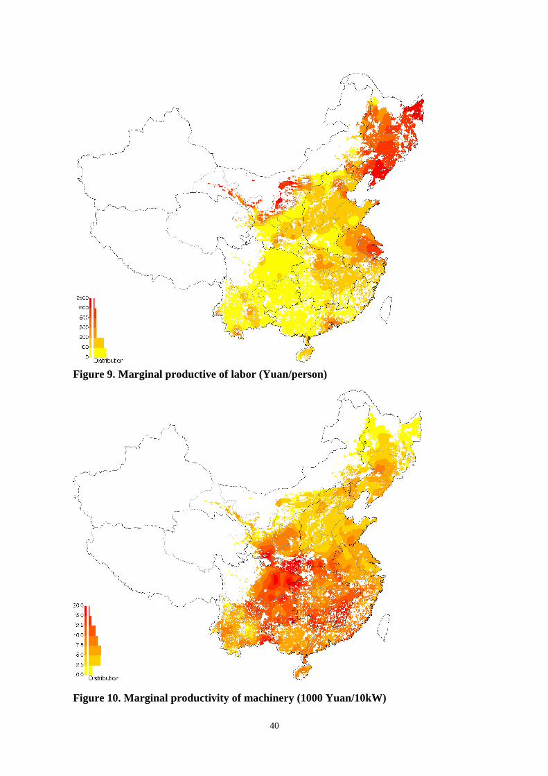
40
Figure 9. Marginal productive of labor (Yuan/person)
Figure 10. Marginal productivity of machinery (1000 Yuan/10kW)
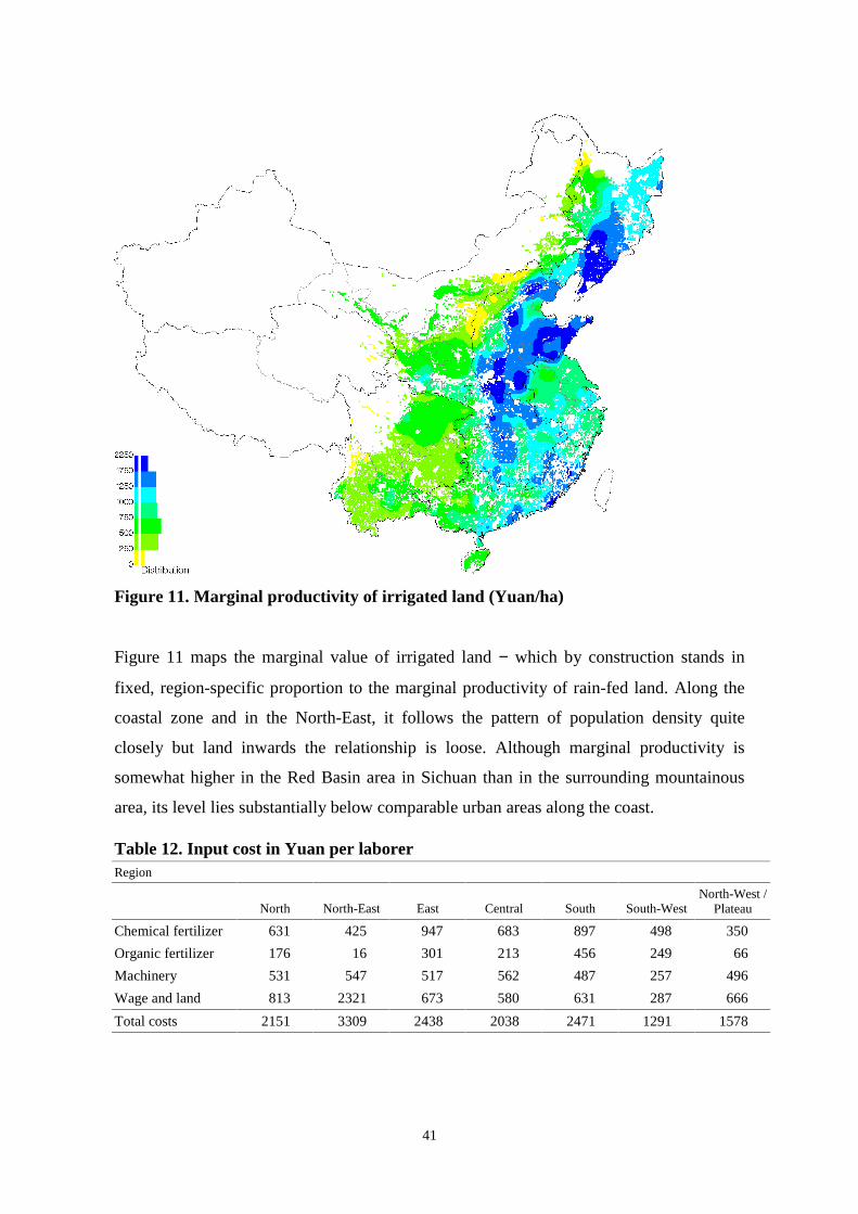
41
Figure 11 maps the marginal value of irrigated land − which by construction stands in
fixed, region-specific proportion to the marginal productivity of rain-fed land. Along the
coastal zone and in the North-East, it follows the pattern of population density quite
closely but land inwards the relationship is loose. Although marginal productivity is
somewhat higher in the Red Basin area in Sichuan than in the surrounding mountainous
area, its level lies substantially below comparable urban areas along the coast.
Table 12. Input cost in Yuan per laborerRegion
North North-East East Central South South-WestNorth-West /
Plateau
Chemical fertilizer 631 425 947 683 897 498 350
Organic fertilizer 176 16 301 213 456 249 66
Machinery 531 547 517 562 487 257 496
Wage and land 813 2321 673 580 631 287 666
Total costs 2151 3309 2438 2038 2471 1291 1578
Figure 11. Marginal productivity of irrigated land (Yuan/ha)

42
At regional level, the average implicit costs (and returns) per laborer for land and wage are
lowest in Central and South-West (see Table 12). In the South-West region, an average
laborer earned in 1990 an income of 287 Yuan. For the coastal regions South, East and
North the earnings for a crop laborer range from 631 Yuan to 813 Yuan on average. This
pattern is in line with the observed out-migration to the coastal provinces during the last
decade. The marginal productivities of labor and land are highest in the northern
provinces.
6. Conclusions
The paper has reported on the specification and estimation of a spatially explicit
transformation function for crop production in China, and indicated that the implicit prices
associated to this function seem compatible with static profit maximization at county level,
at prices that correct for the distance from the main consuming areas. The next step is to
conduct scenario simulations with such a profit-maximizing model, after inclusion of
livestock production and feed demand equation. Then, we will confront these with
consumer demand and balance of payment restrictions, and the final step will be to
incorporate investment into irrigation and solve an inter-temporal welfare model.
43
References
Agricultural Academy of China – Institute of Agricultural Natural Resources and RegionalPlanning (1995), Cultivated Land in China. Beijing: China Agricultural Science Press.
Ash, Robert F. (1997), "The Performance of China's Grain Sector: A RegionalPerspective." In OECD (1997).
Aubert, Claude (1997), "China's Grain Distribution and Price Policy." In OECD (1997),pp. 171-179.
Bierens, H.J. (1987), "Kernel estimators of regression functions." In: Truman F. Bewly(ed.), Advances in Econometrics 1985, New York: Cambridge University Press, pp.99-144.
Bowman, K.O. and L.R. Shenton (1977), "Omnibus Test Contours for Departures fromNormality Based on √b1 and b2 ." Biometrika, 62: 243-250.
Brooke, A., D. Kendrick, and A. Meeraus (1992), GAMS: A User's Guide. Release 2.25.San Francisco: Scientific Press.
Brown, Lester R. and Brain Halweil (1998), "China's Water Shortage Could Shake WorldFood Security." World Watch, July/August, pp. 10-21.
Byrd, William A. (1987), "The Impact of the Two-Tier, Plan/Market System in ChineseIndustry." Journal of Comparative Economics, 11, 2: 295-308.
Byrd, William A. (1989), "Plan and Market in the Chinese Economy: A Simple GeneralEquilibrium Model." Journal of Comparative Economics, 13, 1: 177-204.
Carter, Colin A. and Bin Zhang (1998) “The Wheather Factor and Variability in China’sGrain Supply” , Journal of Comparative Economics, 26, 529-543.
Central Committee of CCP (1985), "Ten Policies of the CCP Central Committee and theState Council for the Further Invigoration of the Rural Economy." In AgriculturalYearbook of China, 1985, Beijing: China's Statistical Publishing House, 1985, pp. 1-3.
Chen, J. Y. and J. Han (1994), "On the China's Rural Reform and Deng Xiaoping's Ideasabout the development of China's Agriculture." China's Rural Economy, no. 10 (Oct.),in Chinese.
Dasgupta, Partha, and Debraj Ray (1986), "Inequality as a Determinant of Malnutritionand Unemployment: Theory." Economic Journal, 96, ?: 1011-1034.
Dasgupta, Partha, and Debraj Ray (1987), "Inequality as a Determinant of Malnutritionand Unemployment: Policy." Economic Journal, 97, 1: 177-188.
Davidson, Russell, and James G. MacKinnon (1993), Estimation and inference ineconometrics. New York, Oxford University Press.
Dazhong, Wen (1993), “Soil erosion and Conservation” , In: Pimentel (eds.), World SoilErosion and Conservation, Cambridge.
Dong, Xiao-yuan (1996), "Two-Tier Land Tenure System and Sustained EconomicGrowth in Post-1978 Rural China." World Development, 24, 5: 915-928.
Eight Ministries and Bureaus – Survey Team of the Costs of Industrial and AgriculturalProducts of State Statistical Bureau, Finance and Price Bureau and Grain Bureau of the

44
Ministry of Commerce, Ministry of Agriculture, Ministry of Forestry, Ministry ofLight Industry, and others (1991), Nationwide Data on Costs and Revenues ofAgricultural Products. Beijing: China Price Publishing House (in Chinese).
Fahlbeck, Erik and Zuhui Huang (1997), "The Property Right Structure of Farmland andFamily Farming in China – An Analysis of Development Options." In OECD (1997),pp. 78-87.
Fan, Shenggen (1991), "Effects of Technological Changes and Institutional Reform onProduction Growth in Chinese Agriculture." American Journal of AgriculturalEconomics, 73, 2: 266-275.
FAO-Food and Agriculture Organization, FAO Fertilizer Yearbook. Rome: FAO (variousissues).
Fischer, Günther, Yuri Ermoliev, Michiel A. Keyzer and Cynthia Rosenzweig (1996),"Simulating the Socio-economic and Biogeophysical Driving Forces of Land-use andLand-cover change: The IIASA Land-use Change Model." Working Paper WP-96-010, International Institute for Applied Systems Analysis, Laxenburg, Austria.
Fischer, Günther and Harry T. van Velthuizen (1996), "Climate Change and GlobalAgricultural Potential Project: A Case Study of Kenya." Working Paper WP-96-71,International Institute for Applied Systems Analysis, Laxenburg, Austria.
Fischer, Günther, Yufeng Chen and Laixiang Sun (1998), "The Balance of CultivatedLand in China During 1988-1995." Interim Report IR-98-047/August, InternationalInstitute for Applied Systems Analysis, Laxenburg, Austria.
Fischer, Günther, Harry T. van Velthuizen and F.O. Nachtergaele (2000), "Global Agro-Ecological Zones Assessment: Methodology and Results." Interim Report IR-00-064,International Institute for Applied Systems Analysis, Laxenburg, Austria.
Gallant, Ronald A. (1987). Nonlinear Statistical Models, New York, John Wiley & Sons.
Halbrendt, Catherine, and Conrado Gempesaw (1990), "A Policy Analysis of China'sWheat Economy." American Journal of Agricultural Economics, 72, 2: 268-278.
Hasenkamp, Georg (1976), Specification and Estimation of Multiple-Output ProductionFunctions. Berlin: Springer-Verlag.
Hayami, Yujiro and Vernon W. Ruttan (1985), Agricultural Development: AnInternational Perspective. Baltimore: The Johns Hopkins University Press.
Huang, Jikun and Linxiu Zhang (1997), "The Macroeconomic and Public ExpenditureImplications of Grain Policies in China: Some Selected Issues for Discussion." InOECD (1997), pp. 180-189.
Kenny, G.J., Harrison, P.A., and Parry, M.L. (eds.), 1993. The effect of climate change onagricultural and horticultural potential in Europe. Environmental Change Unit,University of Oxford.
Keyzer, M.A. (1998), "Formulation and Spatial Aggregation of Agricultural ProductionRelationships within the LUC Model." Interim Report IR-98-092/October,International Institute for Applied Systems Analysis, Laxenburg, Austria.
Keyzer, M.A. and B.G.J.S. Sonneveld (1997). "Using the mollifier method to characterizedata sets and models: the case of the Universal Soil Loss Equation." ITC Journal 97(3-4), 263-272.

45
Kueh, Yak-Yeow (1984), "China’s New Agricultural Policy Program: Major EconomicConsequences, 1979-1983." Journal of Comparative Economics, 8, 2 (June): 353-375.
Kung, James K. (1995), "Equal Entitlement versus Tenure Security under a Regime ofCollective Property Rights: Peasants’ Preference for Institutions in Post-reformChinese Agriculture." Journal of Comparative Economics, 21, 1 (Aug.): 82-111.
Leibenstein, H. (1957), Economic Backwardness and Economic Growth: Studies in theTheory of Economic Development. New York: Wiley.
Lindert, Peter H. (1999) “The Bad Earth? China’s Soils and Agricultural Developmentsince the 1930s” , Economic Development and Cultural Change, 47, 4:701-736.
Lin, Justin Y. (1989), "Rural Factor Markets in China: After the Household ResponsibilitySystem Reform." In B. Reynolds (ed.), Chinese Economic Policy: Economic Reformat Midstream. New York: Paragon House, pp. 169-203.
Lin, Justin Y. (1992), "Rural Reforms and Agricultural Growth in China." AmericanEconomic Review, 82, 1 (March): 34-51.
Lin, Justin Y. (1993), "Government Procurement Price and Rice Supply Response inChina." Paper presented in the Rice Demand and Supply Workshop, International RiceResearch Institute, Philippines.
Lin, Justin Y. (1997), "The Role of Agriculture in the Transition Process in China." InJonathan Kydd, Sophia Davidova, Miranda Mackay and Thea Mech (eds.), The Roleof Agriculture in the Transition Process Towards a Market Economy, UN/ECEEconomic Studies No. 9, New York and Geneva: United Nations, pp. 63-75.
Lin, Nan (1995), "Local Market Socialism: Local Corporatism in Action in Rural China."Theory and Society, 24, 3: 301-354.
McMillan, John, John Whalley and Lijing Zhu (1989), "The Impact of China's EconomicReforms on Agricultural Productivity Growth." Journal of Political Economy, 97: 781-807.
Mendelsohn, Robert, William D. Nordhaus, and Daigee Shaw (1994), "The Impact ofGlobal Warming on Agriculture: A Ricardian Analysis." American Economic Review,84, 4: 753-771
Ministry of Agriculture – Study Group of Rural Cooperative Economy (1988), "A Surveyof Contractual Arrangements and Cooperative Organization in Rural China." Issues inAgricultural Economy (Nongcun Jingji Wenti), no. 8 (Aug.): 33-40.
Ministry of Agriculture – Study Group of Rural Cooperative Economy (1991), "A Surveyof Contractual Arrangements and Cooperative Organization in Rural China." Issues inAgricultural Economy (Nongcun Jingji Wenti), no. 8 (Aug.): 33-40.
Ministry of Water Conservation (1991-1995), Water Conservation Yearbook of China,1990-1994. Beijing: Hydraulic and Electric Publishing House, 1991-1995.
Moene, Karl O. (1992), "Poverty and Land Ownership." American Economic Review, 82,1: 52-64.
Moll, Peter G. (1988), "Transition to Freehold in the South African Reserves."WorldDevelopment, 16, 3: 349-360.

46
OECD (1997), Agricultural Policies in China. Paris: Organization for Economic Co-operation and Development.
Pinstrup-Andersen, Per, Rajul Pandya-Lorch, and Mark W. Rosegrant (1999), World foodprospects: critical issues for the early twenty-first century. IFPRI, Washington, D.C.
Ratkowsky, David A. (1983), Nonlinear Regression Modeling: A Unified PracticalApproach. New York: Marcel Dekker, Inc..
Research Team of Rural Cooperative Economies (1993), "A Survey of the Operation ofChina’s Land Contract System and Cooperative Organizations." Issues in AgriculturalEconomy (Nongcun Jingji Wenti), no. 11 (Nov.): 45-53.
Rosenzweig, C. and Iglesias, A. (eds.) 1994. Implications of climate change forinternational agriculture crop modeling study. U.S. Environmental Protection Agency,EPA 230-B-94-003, Washington, D.C.
Rosenzweig, Cynthia, Ana Iglesias, Günther Fischer, Yanhua Liu, Walter Baethgen, andJames W. Jones (1998), "Wheat Yield Functions for Analysis of Land-use Change inChina." Working Paper, LUC Project, International Institute for Applied SystemsAnalysis, Laxenburg, Austria.
Rozelle, Scott and Echo H. Liang (1992), "Contracts and Choices: Decision Making inPost-reform Rural China." Paper presented at the AAEA/CAEA jointly sponsoredConference on Chinese Agricultural Development in the 1990s, Beijing, China.
Rural Sample Survey Office, Ministry of Agriculture and the Policy Study Office of theCentral Committee of the CCP (1994), "The China's Peasants in the MarketizationProcess: A Survey of Peasant Households and Markets." China's Rural Economy, no. 2(Feb.): 37-43, in Chinese.
Shapiro, S.S. and M.B. Wilk (1965), "An analysis of variance test for normality (completesamples)," Biometrika, 52, 591-611.
Shaw, D. E. and D. A. Griffiths (1979), "Likelihood Ratio and Exact Confidence Regionsin Nonlinear Regression." Symposium on Regression Analysis, Statistical Society ofAustralia, N. S. W. Branch, August 30-31, 1979.
Sicular, Terry (1988), "Plan and Market in China's Agricultural Commerce." Journal ofPolitical Economy, 96, 2: 283-307.
SSB-State Statistical Bureau (1989-1997), Statistical Yearbook of China, 1989-1997.Beijing: China Statistical Publishing House, 1989-1997.
SSB-State Statistical Bureau, Survey Team of Urban Socio-Economy (1992b), Yearbookof Price Statistics of China, 1992. Beijing: China Statistical Publishing House (inChinese).
SSB and CDR- State Statistical Bureau and Center for Development Studies of the StateCouncil (eds.) (1996), County Economies of China (four volumes). Beijing: ChinaStatistical Publishing House (in Chinese).
Stone, B. and G. Desai (1989), "China and India: A Comparative Perspective on FertilizerPolicy Requirements for Long-term Growth and Transitional Needs." In J. W.Longworth (ed.), China's Rural Development Miracle with International Comparisons.Queensland: University of Queensland Press, pp. 274-293.

47
UN (1997), China: Water Resources and Their Use. ST/ESCAP/1762, United Nations.New York: United Nations.
Wang, Lixian (1998) “Mountain Watershed Management in China” , In: H.P. Blume, H.Eger, E. Fleischhauer, A. Hebel, C. Reij and K.G. Steiner (eds), Towards sustainableland use. Advances in geoecology 31. pp. 1017-1021. Catena Verlag, Reiskirchen,Germany.
Wang, Qingbin, Catherine Halbrendt and Stanley R. Johnson (1996), "Grain Productionand Environmental Management in China's Fertilizer Economy." Journal ofEnvironmental Management, 47, 2: 283-296.
Wang, X. Y. (1993), "On the Mechanism of Land Circulation." China's Rural Economy,no. 10 (Oct.), in Chinese.
Wen, Guanzhong J. (1993), "Total Factor Productivity Change in China's Farming Sector:1952-1989." Economic Development and Cultural Change, 42, 1 (Oct.): 1-41.
Wiemer, Calla (1994), "State Policy and Rural Resource Allocation in China as SeenThrough a Hebei Province Township, 1970-85." World Development, 22, 6: 935-947.
World Bank (1985), China: Agriculture to Year 2000. Washington D.C.: The World Bank.
World Bank (1997), China 2020: Food Security Options – At China's Table. WashingtonD. C.: World Bank.
Xie Jungi and Jia Keijing (1994), Potential assessment of crop production. China's LandResources, Use and Productivity Assessments. Technical Report of ProjectCPR/87/029, Vol. III. Beijing.
Ye, Qiaolun and Scott Rozelle (1994), "Fertilizer Demand in China's ReformingEconomy." Canadian Journal of Agricultural Economics, 42, 2: 191-207.
Zhang, Wenfang and Jack Makeham (1992), "Recent Developments in the Market forRural Land Use in China." Land Economics, 68, 2 (May): 139-162.

48
Appendix I:
Description of the estimation procedure and calculation of partial
derivatives for the Taylor expansion approach
The transformation function described in Sections 3.2 and 3.3 can be written in more
compact form as:
Ql(Y, M; α0, α, µ) = C
lG
l(V, A, (x)y ; θ, ρ, β, γ, δ),
where Greek symbols refer to parameters that should be estimated or fixed. On the output
side Ql is a combination of a sum of crop-mix constants and a CES:
0
0
1/
ccc )Y(1
αα
α
µ+= ∑∑ lll
mmmMQ , (I.1)
and on the input side Cl is the sum of cropping zone constants
∑ζ=z
zzZCll
,
while Gl is the generalised Mitscherlich-Baule function:
( ) ( )δ∏ ρδγβ= θ (x);y,AN);;A,VfGj
jlllll
,, (I.2)
with
lll
ll
lll
lll
yHN
and AH
)H(Vw
))/Hw(V(1f
sss
1
jkkkj
jj
j
j
=
δ=
γ=
−β−−=
∑
∑ρ
∈
ρ/
/
exp
Index � stands for counties, m for crop-mix, c for crops, z for multiple cropping zones, s
for land use types, j for input groups, and k for inputs. Estimation is performed by each of
seven regions.

49
Numerical implementation of the estimation procedure
As the estimation problem to be solved is highly nonlinear and nonconvex in parameters,
and relatively large and complex in parameters, it cannot be solved by invoking a standard
numerical optimization procedure. Therefore, it was necessary to develop an iterative
procedure, which operates in five steps:
1. Generation of the initial quantitieslll
/HQq~~ = as data for the separate estimation of the
input and the output function. Calculation of lll
HYy /= .
2. Iterative estimation of parameters of the input function 1HGCq ε+⋅=llll
/~ by linear
regression using a first-order Taylor expansion of the function, which is adjusted until
convergence. This provides good initial estimates for 3.
3. Further estimation of the parameters of the input function in the original nonlinear
form.
4. Estimation of parameters of the output function 2HQq ε+=lll
/~ in the nonlinear
form, for fixed substitution parameter α0.
5. Update the quantity index l
q~ and go to Step 3 until convergence.
Thus, Steps 1-2 constitute the initialization and Steps 3-5 the actual estimation. We note
that a free nonlinear regression would do without separate data for the quantity index, but
attempts to relax this restriction causes convergence problems in the estimation. It should
be added that since the estimation problem is non-convex, only a stationary point could be
obtained which appears to be a local optimum. The robustness of this estimate was tested
by checking convergence to the optimal value after shocks and also by assessing the
resulting change in the other parameters in the calculation of the likelihood ratios (which
performs new rounds of least squares while iteratively setting parameters at half their
originally estimated value). We conclude with some additional remarks on the various
steps:
Step 1. The initial county-level output index l
Q~
is calculated based on the available
provincial prices rcP , the national prices cP and the county-level crop outputs cY� . The
50
provincial crop output rcY is the sum of the county level outputs. A provincial output price
index irP is calculated as
∑∑
=c rcc
c rcrci
r YP
YPP
to measure the departure of the provincial price level from the national one. This provincial
level price index, together with provincial level output prices, is applied to all counties � in
province r, yielding a country-level output index �Q~
.
i
ccc
PPYQllll
/~
∑=
Step 2. The Taylor expansion uses two matrices e and pe of dimension z×ψ. Let subscript p
denote the results of the previous iteration. Using the definitions of (I.1) and (I.2), the sum of
squared disturbances el(z;ψ) can be written as:
lllllll)/H;y,A,V)G(;(ZCQ)(z;e kjjjlssjzz γρβθζ−=ψ ,,, (I.3)
and the derivatives are:
a) partial derivative with respect to ζz:
lll
l HGZe
zz
/−=∂ζ∂
(I.4a)
b) partial derivative with respect to jθ :
llll
l /HGCfe
jj
log−=∂θ∂
(I.4b)
c) partial derivative with respect tojβ :
lll
l
ll HGCf
f1e
j
jj
j
/−
θ−=∂β∂
(I.4c)

51
d) partial derivative with respect tojρ :
lll
l
lll
l
lll HGCw
)vv(w
f
f1wej
jj
j
jkkkk
j
j
j
j
j
jj
j
/
loglog
∑ γ−
ρ−
ρθ−
=∂ρ∂
ρ∈
ρρ
(I.4d)
with lll
HVv kk /=
e) partial derivative with respect to jk,k ∈γ :
lllll
l
ll HGCvw1
f
f1ejj
j1j
jj
jj
j
/ρρ−
ρ−
θ−=∂γ∂
(I.4e)
Step 3. To avoid parameters drifting away in course of the estimation, the parameters ζ, θ, ρ
and η are estimated keeping the others fixed, and next the parameters β and γ are estimated
keeping ζ, θ, ρ and η fixed. The parameters are updated until convergence is reached. The
update procedure of the parameters and convergence level are the same as in Step 2.
Step 4. The parameter α0 is estimated by scanning over the interval [1.5, 2].
Step 5. Convergence is reached when two full rounds lead to less than 0.1 percent change
of the sum of squares of
−lllll
�
HGCHQ /ˆˆ/ˆ .
The entire estimation procedure was implemented in GAMS* (Brooke et al., 1992). The
databases for estimation of the output and input response functions were stored and
managed as MS-Excel worksheets. The statistical software package SAS was used to
transfer the basic data into GAMS format, with a proper declaration and initialization of
sets in GAMS syntax. The resulting database in GAMS format was stored with the save
option "s = ..\data", so that it can be used by the different parts of the GAMS programs
independently using the restart option "r = ..\data".
* The acronym GAMS stands for General Algerbraic Modeling System. GAMS provides a high-levellanguage for compact representation (and documentation) of large and complex optimization models.

52
Appendix II
Output elasticities of input k and land input s, and of crop c
Output elasticity with respect to inputkVl
:
j
j
H
Vw
f
f1
G
V
V
G k1jkj
j
jk
k
ρρ−
γθ
−=
∂∂
l
l
l
l
l
l
l
l
l (II.1)
Output elasticity with respect to land input of types
Al
:
∑
−θ−
δ=
∂∂
jj
j
jj
sss
s
wf
f11
H
A
G
A
A
Gl
l
l
l
l
l
l
l
l (II.2)
Output elasticity with respect to cropcYl
:
∑ αα
=∂∂
α
α
ccc
ccc
c0
0
)Y(
)Y(
Q
Y
Y
Q
l
l
l
l
l
l (II.3)