ESTIMATION OF DISTRIBUTION ALGO- RITHMSccottap/papers/capitulo18.pdf · ESTIMATION OF DISTRIBUTION ALGO-RITHMS A New Tool for Evolutionary Computation Edited by P. LARRANAGA~ J.A

ESTIMATION OF DISTRIBUTION ALGO-RITHMS

ESTIMATION OF DISTRIBUTION ALGO-RITHMSA New Tool for Evolutionary Computation

Edited by

P. LARRANAGA

J.A. LOZANOUniversity of the Basque Country

Kluwer Academic PublishersBoston/Dordrecht/London

Contents

List of Figures vii

List of Tables ix

1Adjusting Weights in Artificial Neural Networks using Evolutionary

Algorithms1

Carlos Cotta, Enrique Alba R. Sagarna, P. Larranaga1. Introduction 22. An Evolutionary Approach to ANN Training 33. Experimental Results 84. Conclusions 14

References 15

v

List of Figures

1.1 The weights of an ANN are encoded into a linear binarystring in GAs, or into a 2k-dimensional real vector in ESs (kweights plus k stepsizes). The EDA encoding is similar tothat of the ES, excluding the stepsizes, i.e., a k-dimensionalreal vector. 6

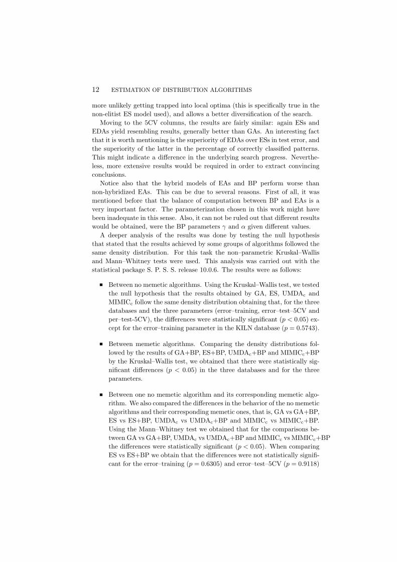
1.2 Convergence plot of different EAs on the KILN database. 13

vii

List of Tables

1.1 Results obtained with the BC database. 101.2 Results obtained with the ECOLI database. 111.3 Results obtained with the KILN database. 11

ix

Chapter 1

Adjusting Weights in Artificial Neural Networksusing Evolutionary Algorithms

Carlos Cotta, Enrique AlbaDepartment of Computer ScienceUniversity of Malaga{ccottap, eat}@lcc.uma.es

R. Sagarna, P. LarranagaDepartment of Computer Science and Artificial IntelligenceUniversity of the Basque Country{ccbsaalr, ccplamup}@si.ehu.es

Abstract Training artificial neural networks is a complex task of great practicalimportance. Besides classical ad-hoc algorithms such as backpropaga-tion, this task can be approached by using evolutionary computation,a highly configurable and effective optimization paradigm. This chap-ter provides a brief overview of these techniques, and shows how theycan be readily applied to the resolution of this problem. Three popu-lar variants of evolutionary algorithms –Genetic Algorithms, EvolutionStrategies and Estimation of Distribution Algorithms– are describedand compared. This comparison is done on the basis of a benchmarkcomprising several standard classification problems of interest for neuralnetworks. The experimental results confirm the general appropriatenessof evolutionary computation for this problem. Furthermore, EvolutionStrategies seem particularly proficient techniques in this optimizationdomain, being Estimation of Distribution Algorithms a competitive ap-proach as well.

Keywords: Evolutionary Algorithms, Artificial Neural Networks, Supervised Train-ing, Hybridization

1

2 ESTIMATION OF DISTRIBUTION ALGORITHMS

1. IntroductionArtificial Neural Networks (ANNs) are computational models based on par-

allel processing (McClelland and Rumelhart, 1986). Essentially, an ANN canbe defined as a pool of simple processing units which communicate amongthemselves by means of sending analog signals. These signals travel throughweighted connections between units. Each of these processing units accumu-lates the inputs it receives, producing an output according to an internal ac-tivation function. This output can serve as an input for other units, or canbe a part of the network output. The interest of ANNs resides in the veryappealing properties they exhibit, such as adaptivity, learning capability, andability to generalize. Nowadays, ANNs have a wide spectrum of applicationsranging from classification to robot control or vision (Alander, 1994).

The rough description of ANNs given in the previous paragraph providessome clues on the design tasks involved in the application of ANNs to a par-ticular problem. As a first step, the architecture of the network has to bedecided. Basicly, two major option can be considered: feed-forward networksand recurrent networks. The former model comprises networks in which theconnections are strictly feed-forward, i.e., no unit receives input from a unitto which the former sends its output. The latter model comprises networks inwhich feedback connections are allowed, thus making the dynamical propertiesof the network turning to be important. In this work we will concentrate onthe first and simpler model, feed-forward networks. To be precise, we will con-sider the so-called multilayer perceptron (Rosenblatt, 1959), in which units arestructured into ordered layers, being connections allowed only between adjacentlayers.

Once the architecture of the ANN is restricted to that of a multilayer percep-tron, some parameters such as the number of layers, and the number of unitsper layer must be defined. After having done this, the last step is adjustingthe weights of the network, so as to make it produce the desired output whenconfronted with a particular input. This process is known as training the ANNor learning the network weights1. We will focus on the learning situation knownas supervised training, in which a set of current-input/desired-output patternsis available. Thus, the ANN has to be trained to produce the desired outputaccording to these examples.

The most classical approach to supervised training is a domain-dependenttechnique known as Backpropagation (BP) (Rumelhart et al., 1986). This al-gorithm is based on measuring the total error in the input/output behaviour ofthe network, calculating the gradient of this error, and adjusting the weights inthe descending gradient direction. Hence, BP is a gradient-descent local searchprocedure. This implies that BP is subject to some well-known problems suchas the existence of local-minima in the error surface, or the non-differentiability

Adjusting Weights in Artificial Neural Networks using Evolutionary Algorithms 3

of the weight space. Different solutions have been proposed to this problem,resulting in several algorithmic variants, e.g., see (Silva and Almeida, 1990).A completely different alternative is the use of evolutionary algorithms for thistraining task.

Evolutionary algorithms (EAs) are heuristic search techniques loosely basedon the principles of natural evolution, namely adaptation and survival of thefittest. These techniques have been shown to be very effective in solving hardoptimization tasks with similar properties to the training of ANNs, i.e., prob-lems in which gradient-descent techniques get trapped into local minima, or arefooled by the complexity and/or non-differentiability of the search space. Thiswork will provide a gentle introduction to the use of these techniques for thesupervised training of ANNs. To be precise, this task will be tackled by meansof three different EA models, namely Genetic Algorithms (GAs), EvolutionStrategies (ESs), and Estimation of Distribution Algorithms (EDAs).

The remainder of the chapter is organized as follows. Section 2. addressesthe application of these techniques to the training of an ANN. This section givesa brief overview on the classical BP algorithm, in order to clarify the differenceand distinctiveness of the EA approach, subsequently described. Some basicdifferences and similarities in the application of the several variants of EAsmentioned to the problem at hand are illustrated in this section too. Next, anexperimental comparison of these techniques is provided in Section 3. Finally,some conclusions and directions for further developments are outlined in Section4.

2. An Evolutionary Approach to ANN TrainingAs mentioned in Section 1, this section is intended to provide an overview

of an evolutionary approach to weight adjusting in ANNs. This is done inSubsections 2.2 and 2.3. Previously, a classical technique for this task, theBP algorithm, is described in Subsection 2.1. This description is importantfor the purposes of a further combination of both –evolutionary and classical–approaches.

2.1 The BP algorithm

It has been already mentioned that the BP algorithm is based on determiningthe descending gradient direction of the error function of the network, adjustingthe weights accordingly. It is thus necessary to define the error function in thefirst place. This function is the summed squared error E defined as follows:

E =12

∑

1≤p≤m

Ep =12

∑

1≤p≤m

∑

1≤o≤no

(dpo − yp

o)2, (1.1)


where m is the number of patterns, no the number of outputs of the network,dp

o is the desired value of the o-th output in the p-th pattern, and ypo is the actual

value of this output. This actual value is computed as a function of the totalinput sp

o received by the unit, i.e.,

ypo = F (sp

o) = F (∑

ur→uo

wroypr ), (1.2)

where F is the activation function on the corresponding unit, and r rangesacross the units from which unit o receives input.

The gradient of this error function E with respect to individual weights is

∂E

∂wij=

∑

1≤p≤m

∂Ep

∂wij=

∑

1≤p≤m

∂Ep

∂spj

∂spj

∂wij=

∑

1≤p≤m

∂Ep

∂spj

ypi . (1.3)

By defining δpj = −∂Ep

∂spj, the weight change is

∆wij =∑

1≤p≤m

∆pwij =∑

1≤p≤m

γδpj yp

i , (1.4)

where γ is a parameter called learning rate.In order to calculate the δp

j terms, two situations must be considered: thej-th unit being an output unit or an internal unit. In the former case,

δpj = (dp

j − ypj )F ′(sp

j ) (1.5)

In the latter case, the error is backpropagated as follows:

δpj = −∂Ep

∂spj

= −∂Ep

∂ypj

∂ypj

∂spj

= −∂Ep

∂ypj

F ′(spj ). (1.6)

The term ∂Ep

∂ypj

can be developed as

∂Ep

∂ypj

=∑

uj→ur

∂Ep

∂spr

∂spr

∂ypj

=∑

uj→ur

∂Ep

∂spr

wjr = −∑

uj→ur

δprwjr, (1.7)

where r ranges across the units receiving input from unit j. Thus,

δpj = F ′(sp

j )∑

uj→ur

δprwjr. (1.8)

One of the problems of following this update rule is the fact that someoscillation can take place were γ large. For this reason, a momentum term α isadded, so

∆wij(t + 1) =∑

1≤p≤m

γδpj yp

i + α∆wij(t). (1.9)


This modification notwithstanding, the BP algorithm is still sensitive to theruggedness of the error surface, being often trapped into local optima. Hence,the necessity of alternative search techniques.

2.2 The Basic Evolutionary Approach

EAs can be used for adjusting the weights of an ANN. This approach isrelatively popular, dating back to late 80s – e.g., see (Caudell and Dolan,1989; Montana and Davis, 1989; Whitley and Hanson, 1989; Fogel et al., 1990;Whitley et al., 1990)– and constituting nowadays a state-of-the-art tool forsupervised learning. The underlying idea is making individuals represent theweights of the ANN, using the network error function as a cost function to beminimized (alternatively, an accuracy function such as the number of correctlyclassified patterns could be used as a fitness function to be maximized; thisapproach is rarely used though). Some general considerations must be takeninto account when using an evolutionary approach to ANN training. These arecommented below.

The first topic that has to be addressed is the representation of solutions.In this case, it is clear that the phenotype space F is Rk, where R ⊂ Ris a closed interval [min,max], and k is the number of weights of the ANNbeing trained, i.e., solutions are k-dimensional vectors of real numbers in therange [min,max]. This phenotype space must be appropriately translated toa genotype space G which will depend on the particulars of the EA used. Inthis work we will consider the linear encoding of these weights. Thus, G ≡Gk

w, i.e, each weight is conveniently encoded in an algorithm-dependent way;subsequently, the genotype is constructed by concatenating the encoding ofeach weight into a linear string.

This linear encoding of weights raises a second consideration, the distributionof weights within the string. This distribution is important in connection withthe particular recombination operator used. If this operator breaks the stringsinto large blocks using them as units for exchange (e.g., one-point crossover),this distribution might be relevant. On the contrary, using a recombinationoperator that breaks the string into very small blocks (e.g., uniform crossover)makes the distribution be irrelevant. A good piece of advice is grouping togetherthe input weights for each unit. This way, the probability of transmitting themas a block is increased, in case an operator such as one-point crossover wereused. Obviously, recombination is not used in some EAs, e.g., in EDAs, so thisconsideration should be rendered mute in such a situation.

2.3 Specific EA Details

The basic idea outlined in the previous subsection can be implemented in avariety of ways depending upon the particular EA used. We will now discuss


Figure 1.1 The weights of an ANN are encoded into a linear binary string in GAs,or into a 2k-dimensional real vector in ESs (k weights plus k stepsizes). The EDAencoding is similar to that of the ES, excluding the stepsizes, i.e., a k-dimensionalreal vector.

these implementation details for the EA models mentioned in the previoussection, namely, GAs, ESs and EDAs.

2.3.1 Genetic Algorithms. GAs are popular members of the evolu-tionary-computing paradigm. Initially conceived by Holland (Holland, 1975),these techniques constitute nowadays the most widespread flavor of EAs. Inthe context of traditional GAs, the encoding of solutions is approached viabinary strings. More precisely, m bits are used to represent each single weight;subsequently, the k m-bit segments are concatenated into a `-bit binary string,` = k ·m. This process is illustrated in Fig. 1.1.

This encoding of the network weights raises a number of issues. The firstone is the choice of m (the length of each segment encoding a weight). It isintuitively clear that a low value of m would induce a very coarse discretizationof the allowed range for weights, thus introducing oscillations and slowing downconvergence during the learning process. On the contrary, too large a valuefor m would result in very long strings, whose evolution is known to be veryslow. Hence, intermediate values for m seem to be appropriate. Unfortunately,such intermediate values seem to be problem dependent, sometimes requiringa costly trial-and-error process. Alternatively, advanced encoding techniquessuch as delta coding (Whitley et al., 1991) could be used, although it has to betaken into account that this introduces an additional level of complexity in thealgorithm.

A related issue is the encoding mechanism for individual weights, i.e., pure bi-nary, Gray-coded numbers, magnitude-sign, etc. Some authors have advocatedfor the use of Gray-coded numbers (Whitley, 1999) on the basis of theoreticalstudies regarding the preservation of some topological properties in the result-ing fitness landscape (Jones, 1995). However, the suitability of such analysis tothis problem is barely understood. Furthermore, the disruption caused by clas-sical recombination operators, as well as the effects of multiple mutations persegment being performed (a usual scenario) will dilute with high probabilitythe advantages (if any) of this particular encoding scheme. Hence, no preferredencoding technique can be distinguished in principle.

2.3.2 Evolution Strategies. The ES (Rechenberg, 1973; Schwefel,1977) approach is somewhat different from the GA approach presented in theprevious subsection. As a matter of fact, the relative intricacy of deciding the


representation of the ANN weights in a genetic algorithm contrasts with thesimplicity of the ES approach. In this case, each solution is represented as itis, a k-dimensional vector of real numbers in the interval [min,max] (see Fig.1.1)2.

Associated to each weight wi, a stepsize parameter σi for performing Gaus-sian mutation on each single weight is included3. These stepsizes undergo evo-lution together with the parameters that constitute the solution, thus allowingthe algorithm to self-adapt the way the search is performed.

Notice also that the use of recombination operators (let alone positionalrecombination operators) is often neglected in ESs, thus making irrelevant thedistribution of weights inside the vector.

Some works using ESs in the context of ANN training can be found in(Wienholt, 1993; Berlanga et al., 1999a; Berlanga et al., 1999b).

2.3.3 Estimation of Distribution Algorithms. EDAs, intro-duced by (Muhlenbein and Paaß, 1996), constitute a new tool for evolutionarycomputation, in which the usual crossover and mutation operators have been re-placed by the estimation of the joint density function of the individuals selectedat each generation, and the posterior simulation of this probability distribution,in order to obtain a new population of individuals. For details about differentapproaches the reader can consult Chapter 3 in this book.

When facing the weighting learning problem in the field of ANNs, discreteas well as continuous EDAs may constitute effective approaches to solve it sincethis problem can be viewed as an optimization problem.

If discrete EDAs are used to tackle the problem, then the representation ofthe individuals would be similar to the one previously explained for GAs. Onthe other hand, if continuous EDAs are considered, then the representationwould be analogous to one used by ESs. In the last case the representationis even simpler than for evolutionary strategies as no mutation parameter isrequired.

Works where EDA approaches have been applied to evolve weights in ar-tificial neural networks can be consulted in (Baluja, 1995; Galic and Hohfeld,1996; Maxwell and Anderson, 1999; Gallagher, 2000; Zhang and Cho, 2000).

2.3.4 Memetic Algorithms. Besides the standard operators usedin each of the EA models discussed above, it is possible to consider additionaloperators adapted for the particular problem at hand. It is well-known –andsupported both by theoretical (Wolpert and Macready, 1997) and empirical(Davis, 1991) results– that the appropriate utilization of problem-dependentknowledge within the EA redounds to highly effective algorithms. In this case,this addition of problem-dependent knowledge can be done by means of a localsearch procedure specifically designed for ANN training: the BP algorithm.


The resulting combination of an EA and BP can be described as a hybrid ormemetic (Moscato, 1999) algorithm.

The BP algorithm can be used in combination with an EA in a variety ofways. For example, an EA has been utilized in (Gruau and Whitley, 1993) tofind the initial weights used in the BP algorithm for further training. Anotherapproach is using BP as a mutation operator, that is, as a procedure for mod-ifying a solution (Davis, 1991). Due to the fact that BP is a gradient-descentalgorithm, this mutation is ensured to be monotonic in the sense that the mu-tated solution will be no worse that the original solution. However, care has tobe taken with respect to the amount of computation left to the BP operator.Despite BP can produce better solutions when executed for a longer time, itcan fall within a local optimum, being the subsequent computational effort use-less; moreover, even when BP steadily progressed, the amount of improvementcould be negligible with respect to additional overhead introduced. For thesereasons, it is preferable to keep the BP utilization at a low level (the exactmeaning of “low level” is again a matter of the specific problem being tackled,so no general guideline can be given).

3. Experimental ResultsThis section provides an empirical comparison of different evolutionary ap-

proaches for training ANNs. The details of these approaches, as well as adescription of the benchmark used are portrayed in Subsection 3.2. Next, theresults of the experimental evaluation of these techniques are presented andanalyzed in Subsection 3.3.

3.1 ANNs and Databases

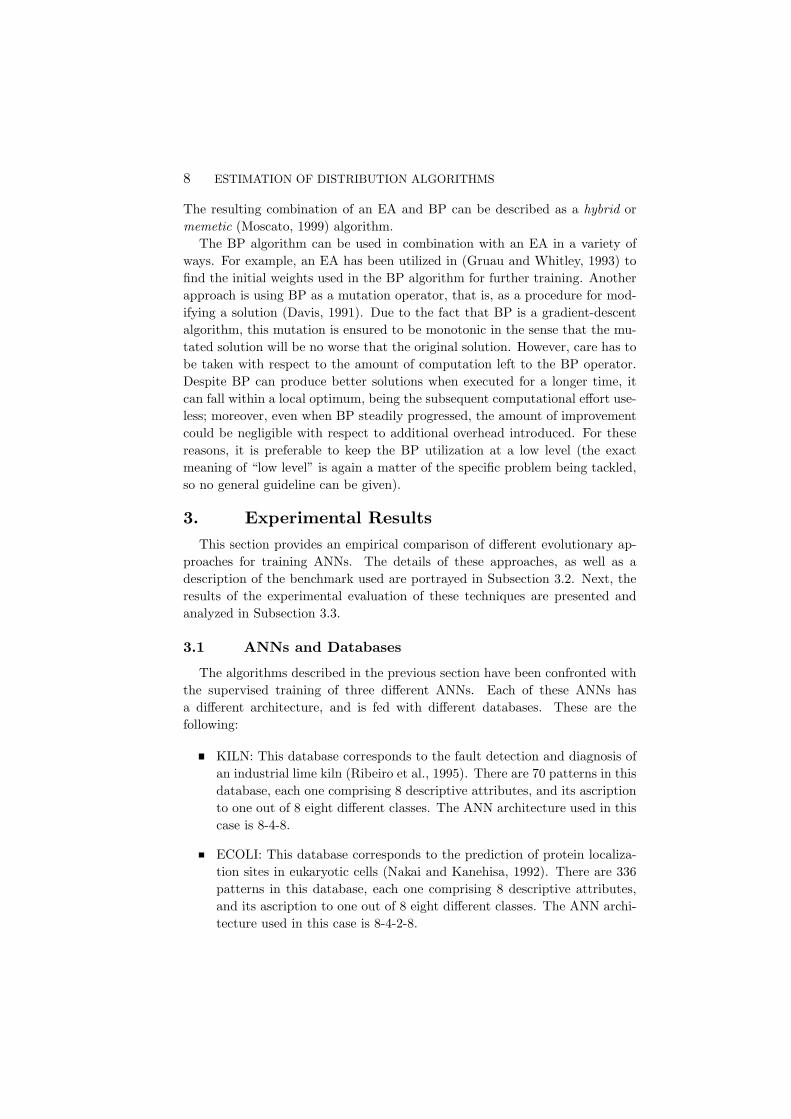
The algorithms described in the previous section have been confronted withthe supervised training of three different ANNs. Each of these ANNs hasa different architecture, and is fed with different databases. These are thefollowing:

KILN: This database corresponds to the fault detection and diagnosis ofan industrial lime kiln (Ribeiro et al., 1995). There are 70 patterns in thisdatabase, each one comprising 8 descriptive attributes, and its ascriptionto one out of 8 eight different classes. The ANN architecture used in thiscase is 8-4-8.

ECOLI: This database corresponds to the prediction of protein localiza-tion sites in eukaryotic cells (Nakai and Kanehisa, 1992). There are 336patterns in this database, each one comprising 8 descriptive attributes,and its ascription to one out of 8 eight different classes. The ANN archi-tecture used in this case is 8-4-2-8.


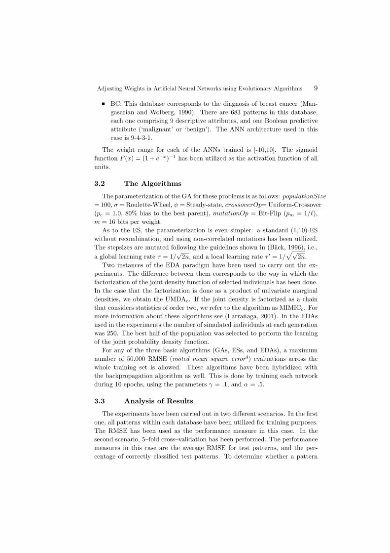
BC: This database corresponds to the diagnosis of breast cancer (Man-gasarian and Wolberg, 1990). There are 683 patterns in this database,each one comprising 9 descriptive attributes, and one Boolean predictiveattribute (‘malignant’ or ‘benign’). The ANN architecture used in thiscase is 9-4-3-1.

The weight range for each of the ANNs trained is [-10,10]. The sigmoidfunction F (x) = (1 + e−x)−1 has been utilized as the activation function of allunits.

3.2 The Algorithms

The parameterization of the GA for these problems is as follows: populationSize

= 100, σ = Roulette-Wheel, ψ = Steady-state, crossoverOp= Uniform-Crossover(pc = 1.0, 80% bias to the best parent), mutationOp = Bit-Flip (pm = 1/`),m = 16 bits per weight.

As to the ES, the parameterization is even simpler: a standard (1,10)-ESwithout recombination, and using non-correlated mutations has been utilized.The stepsizes are mutated following the guidelines shown in (Back, 1996), i.e.,a global learning rate τ = 1/

√2n, and a local learning rate τ ′ = 1/

√√2n.

Two instances of the EDA paradigm have been used to carry out the ex-periments. The difference between them corresponds to the way in which thefactorization of the joint density function of selected individuals has been done.In the case that the factorization is done as a product of univariate marginaldensities, we obtain the UMDAc. If the joint density is factorized as a chainthat considers statistics of order two, we refer to the algorithm as MIMICc. Formore information about these algorithms see (Larranaga, 2001). In the EDAsused in the experiments the number of simulated individuals at each generationwas 250. The best half of the population was selected to perform the learningof the joint probability density function.

For any of the three basic algorithms (GAs, ESs, and EDAs), a maximumnumber of 50.000 RMSE (rooted mean square error4) evaluations across thewhole training set is allowed. These algorithms have been hybridized withthe backpropagation algorithm as well. This is done by training each networkduring 10 epochs, using the parameters γ = .1, and α = .5.

3.3 Analysis of Results

The experiments have been carried out in two different scenarios. In the firstone, all patterns within each database have been utilized for training purposes.The RMSE has been used as the performance measure in this case. In thesecond scenario, 5–fold cross–validation has been performed. The performancemeasures in this case are the average RMSE for test patterns, and the per-centage of correctly classified test patterns. To determine whether a pattern


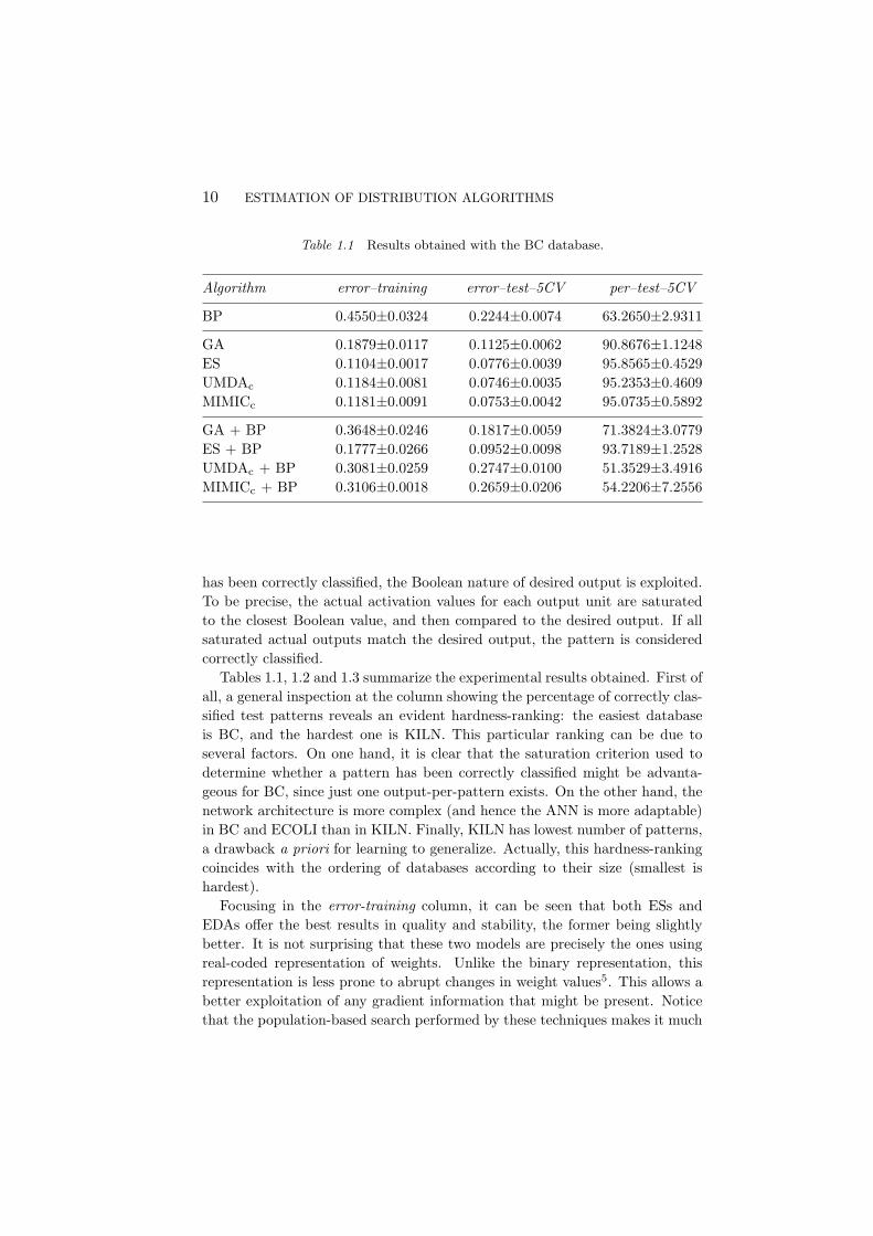
Table 1.1 Results obtained with the BC database.

Algorithm error–training error–test–5CV per–test–5CV

BP 0.4550±0.0324 0.2244±0.0074 63.2650±2.9311

GA 0.1879±0.0117 0.1125±0.0062 90.8676±1.1248ES 0.1104±0.0017 0.0776±0.0039 95.8565±0.4529UMDAc 0.1184±0.0081 0.0746±0.0035 95.2353±0.4609MIMICc 0.1181±0.0091 0.0753±0.0042 95.0735±0.5892

GA + BP 0.3648±0.0246 0.1817±0.0059 71.3824±3.0779ES + BP 0.1777±0.0266 0.0952±0.0098 93.7189±1.2528UMDAc + BP 0.3081±0.0259 0.2747±0.0100 51.3529±3.4916MIMICc + BP 0.3106±0.0018 0.2659±0.0206 54.2206±7.2556

has been correctly classified, the Boolean nature of desired output is exploited.To be precise, the actual activation values for each output unit are saturatedto the closest Boolean value, and then compared to the desired output. If allsaturated actual outputs match the desired output, the pattern is consideredcorrectly classified.

Tables 1.1, 1.2 and 1.3 summarize the experimental results obtained. First ofall, a general inspection at the column showing the percentage of correctly clas-sified test patterns reveals an evident hardness-ranking: the easiest databaseis BC, and the hardest one is KILN. This particular ranking can be due toseveral factors. On one hand, it is clear that the saturation criterion used todetermine whether a pattern has been correctly classified might be advanta-geous for BC, since just one output-per-pattern exists. On the other hand, thenetwork architecture is more complex (and hence the ANN is more adaptable)in BC and ECOLI than in KILN. Finally, KILN has lowest number of patterns,a drawback a priori for learning to generalize. Actually, this hardness-rankingcoincides with the ordering of databases according to their size (smallest ishardest).

Focusing in the error-training column, it can be seen that both ESs andEDAs offer the best results in quality and stability, the former being slightlybetter. It is not surprising that these two models are precisely the ones usingreal-coded representation of weights. Unlike the binary representation, thisrepresentation is less prone to abrupt changes in weight values5. This allows abetter exploitation of any gradient information that might be present. Noticethat the population-based search performed by these techniques makes it much


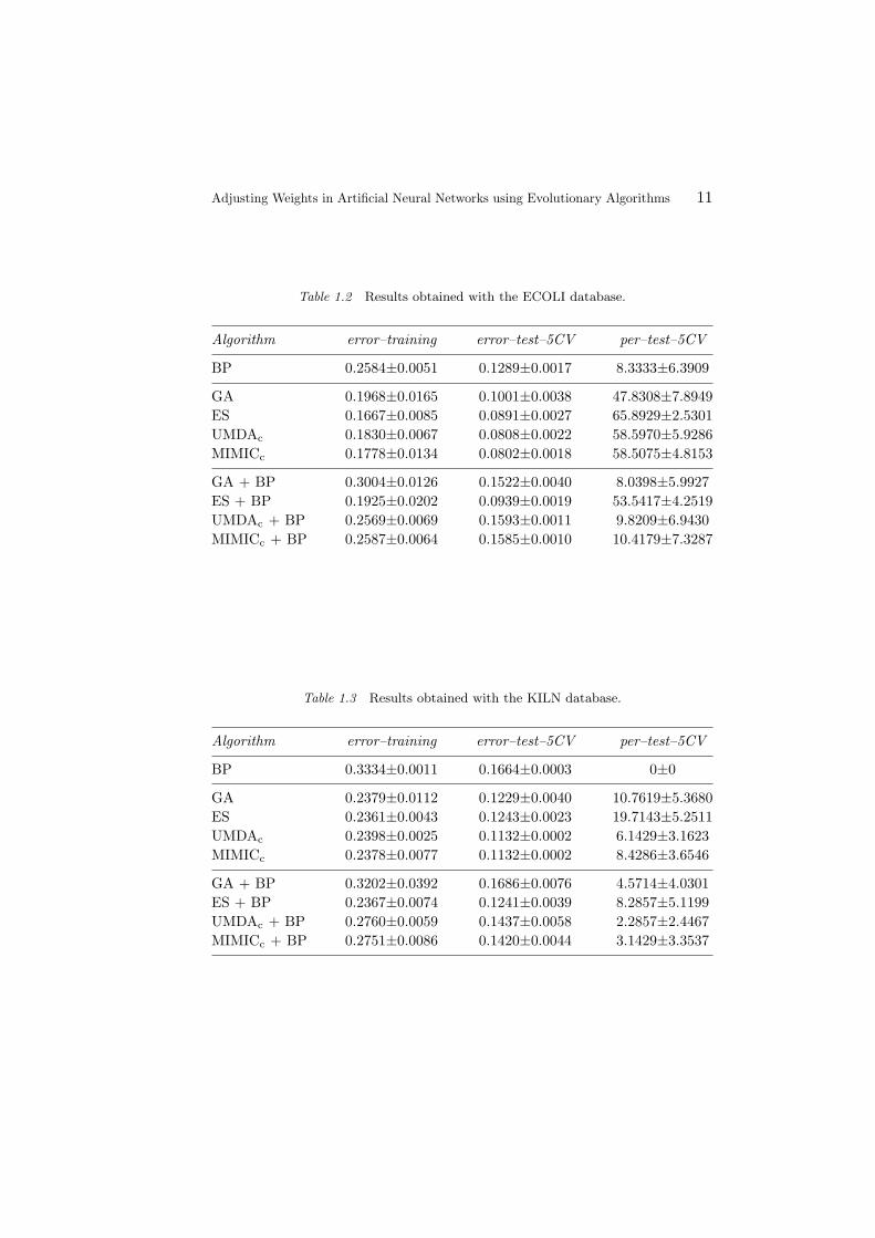
Table 1.2 Results obtained with the ECOLI database.


BP 0.2584±0.0051 0.1289±0.0017 8.3333±6.3909



Table 1.3 Results obtained with the KILN database.


BP 0.3334±0.0011 0.1664±0.0003 0±0




more unlikely getting trapped into local optima (this is specifically true in thenon-elitist ES model used), and allows a better diversification of the search.

Moving to the 5CV columns, the results are fairly similar: again ESs andEDAs yield resembling results, generally better than GAs. An interesting factthat it is worth mentioning is the superiority of EDAs over ESs in test error, andthe superiority of the latter in the percentage of correctly classified patterns.This might indicate a difference in the underlying search progress. Neverthe-less, more extensive results would be required in order to extract convincingconclusions.

Notice also that the hybrid models of EAs and BP perform worse thannon-hybridized EAs. This can be due to several reasons. First of all, it wasmentioned before that the balance of computation between BP and EAs is avery important factor. The parameterization chosen in this work might havebeen inadequate in this sense. Also, it can not be ruled out that different resultswould be obtained, were the BP parameters γ and α given different values.

A deeper analysis of the results was done by testing the null hypothesisthat stated that the results achieved by some groups of algorithms followed thesame density distribution. For this task the non–parametric Kruskal–Wallisand Mann–Whitney tests were used. This analysis was carried out with thestatistical package S. P. S. S. release 10.0.6. The results were as follows:

Between no memetic algorithms. Using the Kruskal–Wallis test, we testedthe null hypothesis that the results obtained by GA, ES, UMDAc andMIMICc follow the same density distribution obtaining that, for the threedatabases and the three parameters (error–training, error–test–5CV andper–test-5CV), the differences were statistically significant (p < 0.05) ex-cept for the error–training parameter in the KILN database (p = 0.5743).

Between memetic algorithms. Comparing the density distributions fol-lowed by the results of GA+BP, ES+BP, UMDAc+BP and MIMICc+BPby the Kruskal–Wallis test, we obtained that there were statistically sig-nificant differences (p < 0.05) in the three databases and for the threeparameters.

Between one no memetic algorithm and its corresponding memetic algo-rithm. We also compared the differences in the behavior of the no memeticalgorithms and their corresponding memetic ones, that is, GA vs GA+BP,ES vs ES+BP, UMDAc vs UMDAc+BP and MIMICc vs MIMICc+BP.Using the Mann–Whitney test we obtained that for the comparisons be-tween GA vs GA+BP, UMDAc vs UMDAc+BP and MIMICc vs MIMICc+BPthe differences were statistically significant (p < 0.05). When comparingES vs ES+BP we obtain that the differences were not statistically signifi-cant for the error–training (p = 0.6305) and error–test–5CV (p = 0.9118)


Figure 1.2 Convergence plot of different EAs on the KILN database.

parameters in the KILN database, maintaining the significativity in thedifferences (p < 0.05) in the rest of the databases and parameters.

In the line of the above remarks about parameterization, it is also interestingto consider the situation in which a larger number of RMSE calculations areallowed. To be precise, the convergence properties of any of these algorithmsis concern arousing. A final experiment has been done to shed some light onthis: the convergence in a long (2 · 105 RMSE calculations) run of the differ-ent algorithms considered has been compared. The results are shown in Fig.1.2. Focusing first in the leftmost plot (corresponding to pure evolutionary ap-proaches) it is evident the superiority of ESs in the short term (≤ 104 RMSEcalculations). In the medium term (∼ 5 · 104 RMSE calculations), UMDAc

emerges as a competitive approach. In the long term (∼ 105 RMSE calcula-tions), UMDAc yields the best results, being the remaining techniques fairlysimilar in performance. From that point on, there is not much progress, ex-cept in the GA case, in which an abrupt advance takes place around 1.5 · 105

RMSE calculations. Due to this abruptness, it would be necessary to carry onadditional tests to determine the likelihood of such an event.

The scenario is different in the case of the hybridized algorithms. Thesetechniques seem to suffer from premature convergence to same extent (in ahigh degree in the case of the GA, somewhat lower in the case of the EDAs,and not so severely in the case of the ES). As a consequence, only ES andMIMICc can advance beyond the 104-RMSE-calculation point. In any case,and as mentioned before, more tests are necessary in order to obtain conclusiveresults.


4. ConclusionsThis work has surveyed the utilization of EAs for supervised training in

ANNs. It is a remarkable fact that EAs remain a competitive technique forthis problem, despite their apparent simplicity. There obviously exist very spe-cialized algorithms for training ANNs that can outperform these evolutionaryapproaches but, in the same line of reasoning, it is foreseeable that more sophis-ticated versions of these techniques could again constitute highly competitiveapproaches. As a matter of fact, the study of specialized models of EAs forthis domain is a hot topic, continuously yielding new encouraging results, e.g.,see (Castillo et al., 1999; Yang et al., 1999).

Future research can precisely be directed to the study of such sophisticatedmodels. There are a number of questions that remain open. For example, thereal usefulness of recombination within this application domain is still underdebate. Furthermore, and granting this usefulness, the design of appropriaterecombination operators for this problem is an area in which a lot of workremains to be done. Finally, the lack of theoretical support of some of theseapproaches (a situation that could alternatively be formulated as their excessiveexperimental bias) is a problem to whose solution many efforts have to bedirected.

AcknowledgmentsCarlos Cotta and Enrique Alba are partially supported by the Spanish Comision

Interministerial de Ciencia y Tecnologıa (CICYT) under grant TIC99-0754-C03-03.

Notes1. Network weights comprise both the previously mentioned connection weights, as well

as bias terms for each unit. The latter can be viewed as the weight of a constant saturatedinput the corresponding unit always receives.

2. Although it is possible to use real-number encodings in GAs, such models still lackthe strong theoretical corpus available for ESs (Beyer, 1993; Beyer, 1995; Beyer, 1996). Fur-thermore, crossover is the main reproductive operator in GAs, so it is necessary to definesophisticated crossover operators for this representation (Herrera et al., 1996). Again, ESsoffer a much simpler approach.

3. Some advanced ES models also include covariance values θij to make all perturbationsbe correlated. We have not considered this possibility in this work since we intended to keepthe ES approach simple. On the other hand, notice that the number of these covariancevalues is O(n2), where n is the number of variables being optimized. Thus, very long vectorswould have been required in the context of ANN training.

4. RMSE =√

2Emno

.

5. Of course, this also depends on the particular operators used in the algorithm. Re-combination is a potentially disturbing operator in this sense. No recombination has beenconsidered in these two models though.

References

Alander, J. (1994). Indexed bibliography of genetic algorithms and neural net-works. Technical Report 94-1-NN, University of Vaasa, Department of In-formation Technology and Production Economics.

Back, T. (1996). Evolutionary Algorithms in Theory and Practice. Oxford Uni-versity Press, New York.

Baluja, S. (1995). An empirical comparison of seven iterative and evolutionaryfunction optimization heuristics. Technical Report CMU-CS-95-193, CarnegieMellon University.

Berlanga, A., Isasi, P., Sanchıs, A., and Molina, J. (1999a). Neural networksrobot controller trained with evolution strategies. In Proceedings of the 1999Congress on Evolutionary Computation, pages 413–419, Washington D.C.IEEE Press.

Berlanga, A., Molina, J., Sanchıs, A., and Isasi, P. (1999b). Applying evolutionstrategies to neural networks robot controllers. In Mira, J. and Sanchez-Andres, J., editors, Engineering Applications of Bio-Inspired Artificial Neu-ral Networks, volume 1607 of Lecture Notes in Computer Science, pages516–525. Springer-Verlag, Berlin.

Beyer, H.-G. (1993). Toward a theory of evolution strategies: Some asymptoticalresults from the (1+

, λ)-theory. Evolutionary Computation, 1(2):165–188.Beyer, H.-G. (1995). Toward a theory of evolution strategies: The (µ, λ)-theory.

Evolutionary Computation, 3(1):81–111.Beyer, H.-G. (1996). Toward a theory of evolution strategies: Self adaptation.

Evolutionary Computation, 3(3):311–347.Castillo, P. A., Gonzalez, J., Merelo, J., Prieto, A., Rivas, V., and Romero,

G. (1999). GA-Prop-II: Global optimization of multilayer perceptrons usingGAs. In Proceedings of the 1999 Congress on Evolutionary Computation,pages 2022–2027, Washington D.C. IEEE Press.

Caudell, T. and Dolan, C. (1989). Parametric connectivity: training of con-strained networks using genetic algoritms. In Schaffer, J., editor, Proceed-

15


ings of the Third International Conference on Genetic Algorithms, pages370–374, San Mateo, CA. Morgan Kaufmann.

Davis, L. (1991). Handbook of Genetic Algorithms. Van Nostrand ReinholdComputer Library, New York.

Fogel, D., Fogel, L., and Porto, V. (1990). Evolving neural networks. BiologicalCybernetics, 63:487–493.

Galic, E. and Hohfeld, M. (1996). Improving the generalization performanceof multi-layer-perceptrons with population-based incremental learning. InParallel Problem Solving from Nature IV, volume 1141 of Lecture Notes inComputer Science, pages 740–750. Springer-Verlag, Berlin.

Gallagher, M. R. (2000). Multi-layer Perceptron Error Surfaces: Visualization,Structure and Modelling. PhD thesis, Department of Computer Science andElectrical Engineering, University of Queensland.

Gruau, F. and Whitley, D. (1993). Adding learning to the cellular developmentof neural networks: Evolution and the baldwin effect. Evolutionary Compu-tation, 1:213–233.

Herrera, F., Lozano, M., and Verdegay, J. (1996). Dynamic and heuristic fuzzyconnectives-based crossover operators for controlling the diversity and con-vengence of real coded genetic algorithms. Journal of Intelligent Systems,11:1013–1041.

Holland, J. (1975). Adaptation in Natural and Artificial Systems. University ofMichigan Press, Ann Harbor.

Jones, T. (1995). Evolutionary Algorithms, Fitness Landscapes and Search. PhDthesis, University of New Mexico.

Larranaga, P. (2001). A review on Estimation of Distribution Algorithms. InLarranaga, P. and Lozano, J. A., editors, Estimation of Distribution Algo-rithms: A new tool for Evolutionary Computation. Kluwer Academic Pub-lishers.

Mangasarian, O. and Wolberg, W. H. (1990). Cancer diagnosis via linear pro-gramming. SIAM News, 23(5):1–18.

Maxwell, B. and Anderson, S. (1999). Training hidden Markov models usingpopulation-based learning. In Banzhaf, W. et al., editors, Proceedings of the1999 Genetic and Evolutionary Computation Conference, page 944, OrlandoFL. Morgan Kaufmann.

McClelland, J. and Rumelhart, D. (1986). Parallel Distributed Processing: Ex-plorations in the Microstructure of Cognition. The MIT Press.

Montana, D. and Davis, L. (1989). Training feedforward neural networks usinggenetic algorithms. In Proceedings of the Eleventh International Joint Con-ference on Artificial Intelligence, pages 762–767, San Mateo, CA. MorganKaufmann.

References 17

Moscato, P. (1999). Memetic algorithms: A short introduction. In Corne, D.,Dorigo, M., and Glover, F., editors, New Ideas in Optimization, pages 219–234. McGraw-Hill.

Muhlenbein, H. and Paaß, G. (1996). From recombination of genes to the es-timation of distributions i. binary parameters. In H. M. Voigt, e. a., editor,Parallel Problem Solving from Nature IV, volume 1141 of Lecture Notes inComputer Science, pages 178–187. Springer-Verlag, Berlin.

Nakai, K. and Kanehisa, M. (1992). A knowledge base for predicting proteinlocalization sites in eukaryotic cells. Genomics, 14:897–911.

Rechenberg, I. (1973). Evolutionsstrategie: Optimierung technischer Systemenach Prinzipien der biologischen Evolution. Frommann-Holzboog Verlag,Stuttgart.

Ribeiro, B., Costa, E., and Dourado, A. (1995). Lime kiln fault detection anddiagnosis by neural networks. In Pearson, D., Steele, N., and Albrecht, R.,editors, Artificial Neural Nets and Genetic Algorithms 2, pages 112–115,Wien New York. Springer-Verlag.

Rosenblatt, F. (1959). Principles of Neurodynamics. Spartan Books, New York.Rumelhart, D., Hinton, G., and Williams, R. (1986). Learning representations

by backpropagating errors. Nature, 323:533–536.Schwefel, H.-P. (1977). Numerische Optimierung von Computer–Modellen mit-

tels der Evolutionsstrategie, volume 26 of Interdisciplinary Systems Research.Birkhauser, Basel.

Silva, F. and Almeida, L. (1990). Speeding up backpropagation. In Eckmiller,R., editor, Advanced Neural Computers. North Holland.

Whitley, D. (1999). A free lunch proof for gray versus binary encoding. InBanzhaf, W. et al., editors, Proceedings of the 1999 Genetic and EvolutionaryComputation Conference, pages 726–733, Orlando FL. Morgan Kaufmann.

Whitley, D. and Hanson, T. (1989). Optimizing neural networks using faster,more accurate genetic search. In Schaffer, J., editor, Proceedings of the ThirdInternational Conference on Genetic Algorithms, pages 391–396, San Mateo,CA. Morgan Kaufmann.

Whitley, D., Mathias, K., and Fitzhorn, P. (1991). Delta coding: An iterativesearch strategy for genetic algorithms. In Belew, R. K. and Booker, L. B.,editors, Proceedings of the Fourth International Conference on Genetic Al-gorithms, pages 77–84, San Mateo CA. Morgan Kaufmann.

Whitley, D., Starkweather, T., and Bogart, B. (1990). Genetic algorithms andneural networks: Optimizing connections and connectivity. Parallel Comput-ing, 14:347–361.

Wienholt, W. (1993). Minimizing the system error in feedforward neural net-works with evolution strategy. In Gielen, S. and Kappen, B., editors, Pro-ceedings of the International Conference on Artificial Neural Networks, pages490–493, London. Springer-Verlag.


Wolpert, D. and Macready, W. (1997). No free lunch theorems for optimization.IEEE Transactions on Evolutionary Computation, 1(1):67–82.

Yang, J.-M., Horng, J.-T., and Kao, C.-Y. (1999). Incorporation family com-petition into Gaussian and Cauchy mutations to training neural networksusing an evolutionary algorithm. In Proceedings of the 1999 Congress onEvolutionary Computation, pages 1994–2001, Washington D.C. IEEE Press.

Zhang, B.-T. and Cho, D.-Y. (2000). Evolving neural trees for time series pre-diction using Bayesian evolutionary algorithms. In Proceedings of the FirstIEEE Workshop on Combinations of Evolutionary Computation and NeuralNetworks (ECNN-2000).

Documents

ESTIMATION OF DISTRIBUTION ALGO- RITHMSccottap/papers/capitulo18.pdf · ESTIMATION OF DISTRIBUTION ALGO-RITHMS A New Tool for Evolutionary Computation Edited by P. LARRANAGA~ J.A