Embed Size (px)
Citation preview
132
[Journal of Political Economy, 2004, vol. 112, no. 1, pt. 1]� 2004 by The University of Chicago. All rights reserved. 0022-3808/2004/11201-0004$10.00
Estimation of Educational BorrowingConstraints Using Returns to Schooling
Stephen V. CameronColumbia University and Federal Reserve Bank of New York
Christopher TaberNorthwestern University
This paper measures the importance of borrowing constraints on ed-ucation decisions. Empirical identification of borrowing constraints issecured by the economic prediction that opportunity costs and directcosts of schooling affect borrowing-constrained and unconstrainedpersons differently. Direct costs need to be financed during schooland impose a larger burden on credit-constrained students. By con-trast, gross forgone earnings do not have to be financed. We explorethe implications of this idea using four methodologies: schooling at-tainment models, instrumental variable wage regressions, and twostructural economic models that integrate both schooling choices andschooling returns into a unified framework. None of the methodsproduces evidence that borrowing constraints generate inefficienciesin the market for schooling in the current policy environment. Weconclude that, on the margin, additional policies aimed at improvingcredit access will have little impact on schooling attainment.
For helpful comments we thank Joe Altonji, Shubham Chaudhuri, John Cochrane, TimConley, Steve Levitt, Lance Lochner, Larry Kenny, Bruce Meyer, Craig Olson, Mike Suk-hadwala, two anonymous referees, and seminar participants at Brigham Young University,the Federal Reserve Bank of New York, Massachusetts Institute of Technology, North-western University, Princeton, Rochester, University of Florida, and University of NorthCarolina. We thank Tricia Gladden for superior research assistance and thoughtful com-ments. We also thank Jeff Kling for providing us with his code. For financial support,Taber acknowledges National Science Foundation grant SBR-97-09-873; Cameron ac-knowledges National Science Foundation grants SBR-97-30-657 and SBR-00-80-731 andsupport from the Federal Reserve Bank of New York. The views expressed in this articleare those of the authors and do not necessarily reflect the position of the Federal ReserveBank of New York or the Federal Reserve System.
educational borrowing constraints 133
I. Introduction
Does access to credit influence educational outcomes? The answer tothis question is fundamental to sensible educational policy and to ourunderstanding of intergenerational transmission of inequality, returnsto schooling, economic growth, and many other economic phenomena.Since a direct answer to the question depends on economic variablesdifficult or impossible to measure, this paper explores alternative ap-proaches to identifying and estimating the influence of credit access oneducational choice. The key idea for identification of the role of creditin determining schooling choices is that two types of schooling costs,opportunity costs of schooling (the value of earnings forgone while inschool) and direct costs of schooling (monetary cost of tuition, books,transportation, and board and room if necessary), affect schoolingchoices differently for credit-constrained and unconstrained individuals.Direct costs need financing during periods of school enrollment andpresent a larger challenge to credit-constrained persons. Gross forgoneearnings, by contrast, do not have to be financed during school.1
Empirical implementation of our approach requires distinct measuresof both direct schooling costs and opportunity costs. Following Card(1995b), we use as a proxy for direct costs an indicator variable for thepresence of any college (either a two- or four-year college) in an indi-vidual’s county of residence. Opportunity costs are proxied by measuresof earnings in low-skill industries located in a person’s local labor marketat the time schooling decisions are made. High prevailing wages in thelocal labor market imply high forgone earnings of college attendance.
The paper reports empirical findings from four methodologically dis-tinct econometric approaches to estimating the importance of creditaccess on schooling choice. Each method exploits implied differencesin responses of borrowing-disadvantaged students to direct costs andforgone earnings of students to identify the magnitude of credit con-straints on schooling choice.
The first approach begins by following Lang (1993) and Card (1995a)and estimating returns to education using an instrumental variable ap-proach.2 These authors explain that when the causal effect of schoolingon earnings is heterogeneous in the population, instrumental variabletechniques do not recover the population average payoff to schoolingbut instead estimate the payoff to schooling for those marginal individ-uals whose schooling choices are most affected by changes in the value
1 Gross forgone earnings are defined as the sum of all income earned by a person notattending school. For expositional simplicity, our story abstracts from income studentsearn during school enrollment. Those earnings would enter the model as an offset todirect college costs, and including them affects none of the implications of our model.
2 We use the term “returns to schooling” to denote the coefficient on schooling in alog wage regression. It is not necessarily the internal rate of return.
134 journal of political economy
of the instrument. They argue that the estimated return to schoolingcould be higher than the population average return if instrumentalvariable estimation identifies the return received for the credit-hinderedsubset of the college-going population. Lang terms this phenomenon“discount rate bias.” We take this argument one step further by usingit to develop a test for borrowing constraints based on estimated returnsto schooling using direct costs and opportunity costs of schooling asalternative instruments. Since schooling decisions of borrowing-con-strained students are regulated more by changes in direct schoolingcosts, the population subset that attends college in response to a fall indirect college costs contains a large concentration of credit-disadvan-taged students. As borrowing is costly, credit-disadvantaged persons re-quire a monetary return to college higher than a person of equal abilitywith access to cheap credit. Thus using measures of direct costs as in-struments in wage studies results in high estimated values of schoolingreturns if credit constraints hamper schooling decisions. In the languageof Lang (1993), the “discount rate bias” would be high. By contrast,instrumenting with measures of opportunity costs should lead to smallerestimates of the schooling effect since opportunity costs do not differ-entially deter credit-disadvantaged persons from college. In other words,this estimator has less “discount rate bias.” Therefore, under the as-sumption that instruments for either direct or opportunity costs are freeof ability bias, the presence of borrowing constraints implies that aninstrumental variable estimator based on an instrument for direct costsof schooling recovers estimates of schooling returns larger than thoseobtained when forgone earnings are used as an instrument.
Empirically, this method uncovers no evidence of educational bor-rowing constraints. In fact, the pattern of point estimates from two-stageleast-squares estimates is consistently opposite the pattern predicted ifconstraints mattered.
Our second approach looks directly at schooling attainment. Exploit-ing the implication of our behavioral model that credit-hindered per-sons are more sensitive to direct schooling costs, we study interactionsbetween schooling costs and observable characteristics likely correlatedwith borrowing constraints. This method, too, fails to detect evidenceof differential credit access. The coefficients on the interactions oftenturn up with the wrong sign and are consistently insignificant.
The third approach formalizes the intuition behind the second ap-proach into a structural econometric model of schooling choice. As thismethodology combines information from both schooling returns andschooling choices into a single model, it uses more information andincorporates behavioral restrictions on returns and choices to yield pointestimates of the magnitude of borrowing constraints. This method alsodelivers a framework to make comparisons between a control group of
educational borrowing constraints 135
unconstrained and a comparison group of potentially credit-constrainedpersons after explicitly taking into account differences in forgone earn-ings, schooling costs, and other characteristics. This model and thegeneralization described next are of independent interest and havemethodological value beyond this study. In the application here, thereturn to schooling and the interest rate at which students borrow tofinance their education are assumed to vary across individuals. Borrow-ing rates depend on observed characteristics of individuals.
This method provides the strongest evidence against the importanceof borrowing constraints for educational decisions. The rates at whichindividuals borrow are precisely estimated, and borrowing constraintsare very small.
The fourth approach generalizes the third to allow educational bor-rowing rates and returns to depend on influences unobserved by theeconometrician. Like the instrumental variable approach, identificationis secured from the use of direct costs and indirect costs as exclusionrestrictions. We show formally that these two types of exclusion restric-tions enter the model in different ways and nonparametrically identifythe magnitude of borrowing constraints. Empirically, estimates of thedistribution of borrowing-constrained persons turn out to be degeneratewith no individuals borrowing-constrained.
Our results are consistent across all four approaches: none find evi-dence that borrowing access is an important component of schoolingdecisions. With this finding in mind, however, it is important to un-derscore the limits of our study. First, we cannot directly observe creditaccess for individuals, so identification of the extent of borrowing con-straints is indirect. Second, our empirical findings cannot addresswhether all students in all environments had adequate access to creditfor educational investments. During the period covered by our data,large subsidies to school and college were already in place in the UnitedStates. Given the policy regime, we find no evidence of inefficienciesin the schooling market resulting from borrowing constraints. This find-ing suggests that additional subsidies aimed at improving credit accesswill have little net value and little impact on overall schoolingattainment.
The paper unfolds as follows. Section II provides a review of theliterature, and Section III presents the economic model and frames thediscussion of borrowing constraints in the context of the model. SectionIV describes the data. Section V summarizes empirical findings on thequestion of borrowing constraints from linear regression and instru-mental variable estimates of returns to education and analyses of school-ing attainment. Section VI lays out the structural models and reportsempirical findings. The paper concludes with a summary (Sec. VII).
136 journal of political economy
II. Previous Work
Evidence favoring the idea that borrowing constraints hinder educa-tional progression, particularly at the college level, is based almost en-tirely on well-documented correlations between schooling attainmentand family income and other family characteristics. The step from cor-relation to causation is precarious since family income is also stronglycorrelated with early schooling achievement, where direct costs ofschooling have little role. Recent work by Cameron and Heckman (1998,2001), Shea (2000), and Keane and Wolpin (2001) has attempted tobetter understand the determinants of schooling choices. Using verydifferent empirical approaches, these researchers turn up no evidencethat borrowing constraints hamper college-going or any other schoolingdecision.
The credit constraint question has also surfaced in the recent liter-ature on returns to education. This literature has aimed at recoveringreturns to schooling from wage regressions purged of “ability bias.”Unobserved ability is thought to bias upward least-squares estimates ofreturns to schooling. Using instrumental variable methods to correctfor the bias, researchers have devised a wide variety of different instru-ments and typically find instrumental variable estimates anomalouslylarger than least-squares estimates (Card 1999, 2001). The connectionbetween credit access and measured returns to schooling—a link orig-inally clarified by Becker (1967)—has been investigated by Lang (1993)and Card (1995a) as an explanation for these high instrumental variableestimates. This argument presumes that borrowing constraints are im-portant for schooling decisions.3
By and large, the literature studying determinants of schooling andthe literature on returns to schooling have evolved in isolation fromone another. Both literatures are discussed in the next subsections.4 Fewempirical studies have integrated educational attainment and schoolingreturns into a unified framework. An important exception is the pio-neering work of Willis and Rosen (1979), on which this paper buildsand which is discussed at the beginning of Section III.
3 We use the terms “borrowing constraint” and “credit constraint” synonymously andbroadly to include not only a hard constraint, which prevents any borrowing outside thefamily, but also the more standard case in which interest rates for educational borrowingare higher than market interest rates. Definitions are clarified in Sec. III.
4 Lochner and Monge (2001) extend the literature on borrowing constraints and creditconstraints in a different direction. They present a schooling model in which credit con-straints are endogenous.
educational borrowing constraints 137
A. Literature on Determinants of Educational Attainment
A ubiquitous empirical regularity that emerges from the literature ondeterminants of schooling is the strong correlation between family in-come and schooling attainment. This correlation has been documentedin legions of U.S. data sets covering the entire twentieth century (see,e.g., Mare 1980; Manski and Wise 1983; Hauser 1993; Manski 1993;Kane 1994; Mayer 1997; Cameron and Heckman 1998, 2001; Levy andDuncan 2000) and in data from dozens of other countries in manystages of political and economic development (see, e.g., the studiescollected in Shavit and Blossfeld [1993]).5 Educational financing con-straints have been the popular behavioral interpretation of the school-ing–family income correlation, particularly in studies of collegeattendance.
However, credit access is only one of many possible interpretationsof this correlation. Family income and other family background mea-sures have been found to be correlated with achievement test perfor-mance in elementary and secondary school as well as with schoolingcontinuation choices at all levels of schooling from eighth grade throughgraduate school. Cameron and Heckman (1998, 2001) adopt a “lifecycle” view of the importance of family income and other family factorsand argue that family income is a prime determinant of the string ofearly schooling decisions. They conclude that the measured effect offamily income on continuing college is largely a proxy for its influenceon early achievement.6
Shea’s (2000) findings support this interpretation of the data. Heisolates the component of family income variation that could arguablybe ascribed to “luck,” coming from union status, job loss, and otherfactors, to estimate the causal effect of income on schooling. He findslittle or no correlation between this component of income and chil-dren’s schooling outcomes.7 Keane and Wolpin (2001) take a differentapproach. They estimate a rich discrete dynamic programming modelof schooling, work, and savings. Model simulations reveal that relaxingborrowing constraints has almost no effect on schooling, but these con-straints are important determinants of working during school.
5 Tomes (1981) and Mulligan (1997) are related but look at the elasticity of schoolingto income. They find higher elasticities for families that are more likely to be borrowing-constrained.
6 Carneiro, Heckman, and Manoli (2002) extend this work using similar methods butget different outcomes. They find evidence that suggests that borrowing constraints maydelay entrance and affect college completion and quality.
7 Shea studies extracts from the Panel Study of Income Dynamics and finds no effectsin the full sample. He does find modest evidence of a relationship in the low-incomesubsample, though such a finding is not inconsistent with Cameron and Heckman’s (2001)view that family income effects operate at the earliest stages of schooling.
138 journal of political economy
B. Returns to Education Literature
A large literature in labor economics has been concerned with esti-mating the causal effect of schooling on earnings. Ordinary least squares(OLS) regressions of earnings on schooling have long been believed tobe biased upward as a result of “ability bias”: individuals who attainhigher levels of schooling do so in part because they are smart and earna return on that characteristic as well as on their additional years ofeducation. Empirical evidence for this idea has been found in virtuallyevery data set with pre–labor market measures of scholastic ability, suchas standardized test scores. Including test scores in wage regressionsleads to a decline in the estimated effect of schooling. Nevertheless,scholastic test scores are imperfect measures of earning ability and leavesubstantial scope for bias from unobserved components of ability.
A good deal of recent work uses instrumental variables or relatedtechniques to address the problems caused by omitted ability measures.8
Card (2001) provides an extensive survey of this literature. Contrary tothe intuition provided by the ability bias story, Card documents thatresearchers often find that the estimated coefficient on schooling risesrather than falls when instrumental variable procedures are used. Build-ing on the model in Becker’s (1967) Woytinsky lecture, Lang (1993)and Card (1995a) explore heterogeneity in borrowing rates as an ex-planation for this pattern, which Lang terms “discount-rate bias.”
In Becker’s model, a student invests in schooling until her return isequal to the interest rate she faces. If borrowing-constrained individualsface higher personal interest rates, they will demand higher returnsfrom schooling at the margin. If returns to schooling vary across indi-viduals because of differential credit costs, the pattern of estimates pro-duced by instrumental variable estimators may be explained by the factthat many of these estimators identify the causal effect of schoolingfrom the subset of individuals who are borrowing-constrained and whosereturn to schooling is higher than the population average return. Ifreturns to schooling were homogeneous, instrumental variables wouldyield consistent estimates of the causal effect of education for the pop-ulation. When returns are heterogeneous, instrumental variable esti-mates must be interpreted with care. Imbens and Angrist (1994) showthat instrumental variable estimates measure the treatment effect ofschooling (i.e., the causal effect) for groups whose schooling decisionsare most sensitive to changes in the instrument used in estimation. Forinstance, schooling choices of borrowing-constrained individuals maybe most sensitive to changes in college tuition. Because of their higher
8 Altonji and Dunn (1996) use a somewhat different strategy that is relevant to ourstudy. They look for interactions between the return to schooling and family background.Their results are mixed, but some specifications point to a positive interaction.
educational borrowing constraints 139
costs of raising funds for schooling, borrowing-constrained individualsalso demand the highest returns to continue. Thus the instrumentalvariable estimate of schooling returns when returns are instrumentedwith college costs will be an average of returns for the constrained groupand will be higher than the population average return.9 This argumentalso helps explain patterns of estimates obtained from studies employing“selection” models of schooling. Selection models take into accountability bias, but discount rate bias does not appear. These studies gen-erally report lower estimated returns to education than those obtainedfrom OLS (see, e.g., Willis and Rosen 1979; Taber 2001).
III. The Model
An economic description of schooling choice is developed in this sec-tion. The model illustrates differences in the influence of direct school-ing costs and opportunity costs on the schooling choices of borrowing-hindered and unhindered students. The differential influence of eachtype of cost is essential for identification in all the empirical approachesdeveloped below.
The closest antecedent of our work is the paper by Willis and Rosen(1979), who integrate future returns to education into their analysis ofschooling decisions to account for self-selection into college attendance.Our framework extends their work in two important respects. First, Willisand Rosen study only college-entry decisions among a sample of highschool graduates. We do not condition our sample on the high schoolgraduation decision; rather, we model (1) the decision to complete highschool, (2) the decision to enter college, and (3) the decision to com-plete college. Our analysis avoids the sample selection problem thatarises by conditioning on high school graduation.10
Second, and more important, Willis and Rosen estimate a first-orderlinear approximation of their economic model. By doing so, they con-found the influences of direct and indirect costs of going to college.Separating these influences underlies our strategy to identify and esti-mate the quantitative importance of borrowing constraints.
To avoid inconsistencies between the theoretical and empirical sec-tions of the paper, we keep the specification of the behavioral modeldeveloped in this section as close as possible to the specification of theempirical structural models described in Section VI. The main results
9 Heckman and Vytlacil (1998) present a more complete description of the econometricsbehind Card’s (1995a) model. Angrist and Krueger (1999) also embody the idea of dis-count rate bias into their econometric framework.
10 We are not the first to address this problem (see, e.g., Taber 2001).
140 journal of political economy
derived below hold true in more elegant and general versions of themodel.11
The model begins with a specification of individual preferences. In-dividuals derive utility from consumption and tastes for nonpecuniaryaspects of schooling. These nonpecuniary tastes represent the utility ordisutility from school itself or preferences for the menu of jobs availableat each level of schooling.
Assume that lifetime utility for schooling level S is given by� gcttV p d � T(S), (1)�S
gtp0
where is consumption at time t, represents nonpecuniary tastesc T(S)t
for schooling level S, d is the subjective rate of time preference, and g
is a parameter of utility curvature with a value in (��, 1). Define toSbe the set of possible schooling choices. Individuals choose S out of thisset so that
S p arg max {V FS � S }. (2)S
Much of the schooling literature—including Becker (1967), Rosen(1977), Willis and Rosen (1979), Willis (1986), Lang (1993), and Card(1995a)—models heterogeneity of credit access as a person-specific rateof interest, denoted here as r, at which a person can borrow and savethroughout life. Credit-constrained persons borrow at a high r, whichmakes educational financing costly.
This approach to modeling credit cost heterogeneity has the unat-tractive feature that a high lifetime r implies high returns to savingsafter labor market entry. This in turn implies that giving assets to bor-rowing-constrained individuals prior to college will raise their lifetimewealth but not alter their schooling decisions.12
Our model departs from the literature by adopting the simple butnovel assumption that individuals borrow at their personal rate r whilein school but face a common market interest rate for all borrowing andlending after labor market entry. Confining borrowing rate heteroge-neity to the schooling years is a natural assumption if one considers the
11 The implications of the model depend on borrowing-constrained individuals’ havinghigher marginal utility of income when in school than when out of school. The mainresults go through if credit access is modeled as a hard borrowing constraint (no borrowingoutside the family), as a higher interest rate for students than for nonstudents, or as anincreasing function of the amount borrowed.
12 This result follows because the assumption of a constant lifetime r gives rise to aseparation result that simplifies the model. Given r, individuals choose schooling to max-imize the present value of lifetime earnings. Thus, when interest rates and nonpecuniaryschooling tastes are held fixed, income transfers have no direct effect on schooling choices.In our setup, an increase in income transfers influences schooling choices by raising thenet value of further schooling.
educational borrowing constraints 141
borrowing rate to be determined by the ability to collateralize loanswith personal or family assets during school. The specific form of bor-rowing constraints is not essential to the results in this section. Sinceour data do not have information on consumption or assets, we focuson a simple type of borrowing constraint that is straightforward to es-timate in the structural econometric model described in Section VI.
Define R to be the borrowing rate during school and let denoteR m
the market rate, which is normalized for convenience such that. Students maximize utility subject to the lifetime budget1/R p dm
constraint
S�1 �t S1 1 t�Sc � d c ≤ I , (3)� �t t S( ) ( )R Rtp0 tpS
where S is total years of school and is the present value of incomeIS
net of direct schooling costs. The first-order conditions are
t/(1�g)c p (dR) c , t ≤ S,t 0
S/(1�g)c p (dR) c , t 1 S.t 0
Plugging these values into the budget constraint yields
S�1 �
tg/(1�g) t/(1�g) Sg/(1�g) tI p R d c � (Rd) dc (4)� �S 0 0.tp0 tpS
Finally, solving in terms of and inserting the value into the utilityc It S
function leaves us with the following expression for lifetime utility of aperson choosing S years of school:
1�gS�1 �g tg/(1�g) t/(1�g) Sg/(1�g) tI � R d � (Rd) � d[ ]S tp0 tpS
V p � T(S). (5)Sg
Equation (5) represents the indirect lifetime utility function conditionalon schooling choice S.
We next solve for the present value of income. To focus on borrowingconstraints, we abstract from earnings uncertainty by assuming that earn-ings streams associated with all levels of S are known with certainty attime 0.13 Let be earnings at time t for an individual with S years ofwSt
schooling. Individuals have zero earnings while in school and pay directcost at time to attend schooling level S. Abstracting from labort S � 1S
13 Uncertainty in future returns to education introduces an option value to furthereducation. For instance, even if predicted returns to college completion were low, indi-viduals may still graduate from college in case realized returns outperform predictedreturns (see Taber 2001).
142 journal of political economy
supply decisions, we have the following expression for the present valueof income discounted to time :t p 0
� S�1S t1 1t�SI p d w � t� �S St t�1( ) ( )R RtpS tp0
S�1S t1 1p W � t , (6)�S t�1( ) ( )R Rtp0
where is the present value of earnings associated with schooling levelWS
S discounted to time S.To illustrate the main predictions of the model, consider how changes
in direct costs and opportunity costs affect utility in a world with onlytwo schooling levels, and . Let be the direct cost ofS p 0 S p 1 t1
, and assume that there are no direct costs associated withS p 1 S p. Lifetime utility values for and are given by0 S p 0 S p 1
g 1�gW [1/(1 � d)]0V p � T(0) (7)0g
andg g/(1�g) 1�g[(W /R) � t ] {1 � (Rd) [d/(1 � d)]}1 1V p � T(1). (8)1
g
A person chooses when , and otherwise. ForgoneS p 1 V � V 1 0 S p 01 0
earnings are represented by the wage rate for unskilled ( ) workersS p 0.W0
Tastes for schooling and are not observed by the analystT(0) T(1)but distributed randomly in the population. Conditioning on potentialwages, direct costs, and the borrowing rate, we get
Pr (S p 1FW , W , R, t ) p Pr (V 1 V FW , W , R, t ) (9)1 0 1 1 0 1 0 1
p Pr (D 1 T(0) � T(1)FW , W , R, t ), (10)1 0 1
whereg g/(1�g) 1�g[(W /R) � t ] {1 � (Rd) [d/(1 � d)]}1 1D p
g
g 1�gW [1/(1 � d)]0� . (11)g
Thus, given tastes for education, the larger the D term, the more likelya person completes schooling level . Given this simple relationshipS p 1between D and schooling attendance, we focus our attention on howdirect and opportunity costs of schooling ( and ) influence D.W t0 1
To explore the relationship between direct and opportunity costs and
educational borrowing constraints 143
the value of D, consider two individuals with identical preferences, oneborrowing-constrained and one not, and let for sim-T(1) p T(0) p 0plicity. Suppose that both persons are indifferent between attendingand not attending school, so that . The unconstrained personV p V0 1
borrows at the market rate ; the constrained person borrows atR p 1/d
some rate . Consider each person’s reaction at to a dollarR 1 1/d t p 0increase in the present discounted value of forgone earnings and al-ternatively to a dollar increase in direct schooling costs.
For the person borrowing at the market rate, a dollar is a dollar:changes of equal magnitude in direct costs and opportunity costs havethe same influence on the schooling decision. To see this, notice fromequations (7) and (8) that implies that the present values ofV p V0 1
income for and are equal at time 0: . Hence,S p 0 S p 1 W p W d � t0 1 1
a dollar rise in and a dollar rise in have the same effect on theW t0 1
relative value of :S p 1
�D �gV �gV �D1 0p p p . (12)�t dW � t W �W1 1 1 0 0
By contrast, for the credit-constrained person to be indifferent, equa-tions (7) and (8) show it must be that . Thus a dollarW 1 (1/R)W � t0 1 1
rise in direct costs of school has a larger (in absolute value) influenceon the value of schooling than a dollar drop in forgone earnings:
�V �gV �gV �V1 1 0 0p ! p . (13)�t (1/R)W � t W �W1 1 1 0 0
Put differently, the shadow value of a dollar of income is higher whilein school than while out of school.
The three predictions of the model of interest to us are now statedmore precisely as propositions. Note first that a rise in R reduces thelikelihood that a person chooses as long as she is not a net saverS p 1while in school:14
�D �V gV1 1p p � (c � t ) ! 0, (14)0 1�R �R RI1
where is optimal time 0 consumption.c 0
Proposition 1. A dollar rise in diminishes the value of moret V1 1
14 This is generally true as long as and must hold when schooling costs arec 1 �t0 1
nonnegative.
144 journal of political economy
for the individual with higher R as long as that person is not a net saverduring school:
2� D gV d1 g/(1�g)p � (c � t )(1 � g) � c (Rd) ! 0. (15)0 1 02 [ ]�R�t RI 1 � d1 1
Proposition 2. The influence of on D does not depend on R:W0
2 g�1 1�g� D �W [1/(1 � d)]0p p 0. (16)�R�W �R0
Proposition 3. Consider credit-constrained and unconstrained in-dividuals c and u who are both indifferent about attending college andreceive the same utility if they go to college, so that V p V p0c 1c
. Assume that they have identical nonpecuniary tastes forV p V0u 1u
schooling and that , g, and d are also identical. The “return to edu-t1
cation” for the constrained person is higher than it is for the uncon-strained person. That is, implies .R 1 R W /W 1 W /Wc u 1c 0c 1u 0u
The last implication of the model follows directly from the fact thatamong the conditioning group, a person borrowing at a high R mustbe compensated with a higher to remain indifferent. That is, sinceW1
and and if is higher than , for c and u to�V /�R ! 0 �V /�W 1 0 R R1 1 1 c u
be indifferent, then must be higher than .W W1c 1u
The predictions embodied in these propositions are used in all fourempirical approaches explored in Sections V and VI below. The firsttwo approaches use the economic intuition derived here to guide em-pirical specifications and interpretation of estimated parameters. Thesecond two approaches are based on estimated structural implemen-tations of the behavioral model elaborated here. Econometric identi-fication explicitly requires that and enter the model in differentW t0 1
ways.
IV. The Data
Our analysis is based on black, Hispanic, and white males from the1979–94 waves of the National Longitudinal Survey of Youth (NLSY).Because the NLSY collected detailed information on family background,scholastic achievement, labor market outcomes, county of residence,and school attendance and completion starting at relatively young ages,it is ideal for our study. The NLSY data comprise four distinct samples:a random sample of the population, a random sample of the black andHispanic populations, a sample drawn from the military, and a sampleof the economically disadvantaged, nonblack, non-Hispanic population.
We limit our sample in four ways. First, we exclude from our analysisthe military and the nonblack, non-Hispanic disadvantaged subsamples
educational borrowing constraints 145
because they are not drawn according to exogenously determined char-acteristics.15 Second, we use only males because their schooling and laborsupply decisions are less complicated by fertility and labor market par-ticipation considerations. Third, because information about events oc-curring before January 1978 is retrospective and limited, we confineour sample to males between ages 13 and 16 as of that date in orderto have reliable information on schooling attendance, parental income,and county of residence. County of residence is used to construct mea-sures of labor market conditions and measures of college proximity.Finally, 13 percent of the sample was eliminated because respondentsdid not complete the Armed Services Vocational Aptitude Battery(ASVAB) (see below) or because of missing data in county of residenceduring high school (measured at age 17 when available), family income,or one of the family background variables. Final sample sizes are re-ported in table 1.
We construct panel data from NLSY annual observations. Annual ob-servations on each respondent begin no later than age 16 and extendthrough ages 29–33. For the analysis of wages, we exclude annual wageobservations taken before age 22 because most college graduates werestill in school before that age.16
Summary statistics of the main variables used in the analysis are pre-sented in table 1. Panels A–C show summary statistics of static variablesfor years of schooling completed, racial-ethnic identity, family back-ground, and geographic location measured at age 17. Details of thevariables are provided in the notes to the table.
Panel D shows summary statistics for test score variables. The scoresare taken from the 10-part ASVAB. The test was administered to NLSYrespondents in the summer of 1980, when respondents in our samplewere between ages 15 and 18. The set of four variables word score, mathscore, science score, and automotive score are raw scores on four of theASVAB sections. The variable AFQT score is the score on the ArmedForces Qualification Test, a weighted sum of ASVAB components thatmeasure literacy and basic mathematics skills. This variable has beenwidely used in recent empirical work. The other four test scores areused together in the analysis below as an alternative to AFQT score.Taber (2001) contends that these four scores represent a parsimonious
15 Thus our data include all observations from the random sample and the randomblack and Hispanic oversamples. The military and the nonblack, non-Hispanic disadvan-taged samples are small relative to the data we include. In addition, the military oversamplewas discontinued after the 1984 wave of the NLSY.
16 Starting the panel at an earlier age creates a data set unrepresentative of the popu-lation since it would contain more annual observations for high school dropouts andgraduates than for college graduates. The estimates presented below are not sensitive tohigher age cutoffs.
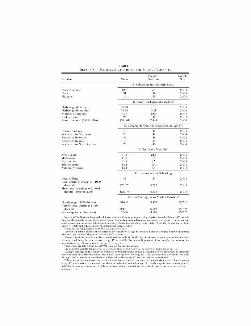
TABLE 1Details and Summary Statistics of the Primary Variables
Variable MeanStandardDeviation
SampleSize
A. Schooling and Minority Status
Years of schoola 12.8 2.5 2,404Black .31 .46 2,404Hispanic .19 .39 2,404
B. Family Background Variablesb
Highest grade father 10.50 4.10 2,404Highest grade mother 10.78 3.21 2,404Number of siblings 3.73 2.63 2,404Broken home .24 .42 2,404Family incomec (1999 dollars) $39,601 2,444 2,404
C. Geographic Controls (Measured at Age 17)
Urban residence .79 .40 2,404Residence in Northeast .20 .40 2,404Residence in South .36 .48 2,404Residence in West .19 .39 2,404Residence in North Central .25 .43 2,404
D. Test Score Variablesd
AFQT score 61.1 22.3 2,404Math score 11.9 6.3 2,404Word score 21.9 8.5 2,404Science score 14.2 5.4 2,404Automotive score 13.4 5.5 2,404
E. Instruments for Schooling
Local collegee .87 .34 2,404Local earnings at age 17 (1999
dollars)f $22,620 4,209 2,404Mean local earnings over work-
ing life (1999 dollars)f $23,073 4,333 2,404
F. Time-Varying Labor Market Variablesg
Hourly wage (1999 dollars) $10.01 3.479 13,762Current local earnings (1999
dollars) $24,519 6,122 13,762Work experience (in years) 7.536 3.169 13,762
Source.—The National Longitudinal Survey of Youth. County average earnings is taken from the Bureau of EconomicAnalysis’s Regional Economic Information System data and constructed from annual average earnings in retail, wholesale,and construction industries. Information on college location and college costs is taken from the Department of Edu-cation’s HEGIS and IPEDS surveys of institutional characteristics.
a Years of schooling completed by the 1994 interview date.b Except for family income, these variables are measured at age 14. Broken home is a binary variable indicating
whether a person was living with both biological parents.c Parental family income is available annually only for individuals who are dependents of their parents. Our measure
takes parental family income as close to age 17 as possible. For about 16 percent of our sample, the measure wasunavailable at age 17 and was taken at age 16 or age 18.
d Test scores are taken from the ASVAB tests; see the text for details.e An indicator variable for presence of a college (two- or four-year) in the county of residence at age 17.f Average earnings in the county in which an individual resides at age 17 among persons employed in industries
predominated by unskilled workers. Mean local earnings over working life is the earnings rate averaged from 1980through 1996 in the county in which an individual resides at age 17. See the text for more details.
g These are annual measures. Current local earnings is an annual measure of the same data series as local earningsat age 17 and is taken in the county in which an individual resided at age 17. Hourly wage is hourly earnings at anindividual’s current or most recent job at the time of each annual interview. Work experience is defined as age �schooling � 6.
educational borrowing constraints 147
set of wage predictors that capture more dimensions of ability thanAFQT by itself.
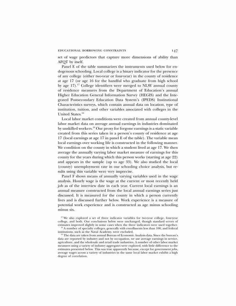
Panel E of the table summarizes the instruments used below for en-dogenous schooling. Local college is a binary indicator for the presenceof any college (either two-year or four-year) in the county of residenceat age 17 (or age 16 for the handful who graduate from high schoolby age 17).17 College identifiers were merged to NLSY annual countyof residence measures from the Department of Education’s annualHigher Education General Information Survey (HEGIS) and the Inte-grated Postsecondary Education Data System’s (IPEDS) InstitutionalCharacteristics surveys, which contain annual data on location, type ofinstitution, tuition, and other variables associated with colleges in theUnited States.18
Local labor market conditions were created from annual county-levellabor market data on average annual earnings in industries dominatedby unskilled workers.19 Our proxy for forgone earnings is a static variablecreated from this series taken in a person’s county of residence at age17 (local earnings at age 17 in panel E of the table). The variable meanlocal earnings over working life is constructed in the following manner.We condition on the county in which a student lived at age 17. We thenaverage the annually varying labor market measure of earnings for thiscounty for the years during which this person works (starting at age 22)and appears in the sample (up to age 33). We also studied the local(county) unemployment rate in our schooling choice analysis, but re-sults using this variable were very imprecise.
Panel F shows means of annually varying variables used in the wageanalysis. Hourly wage is the wage at the current or most recently heldjob as of the interview date in each year. Current local earnings is anannual measure constructed from the local annual earnings series justdiscussed. It is measured for the county in which a person currentlylives and is discussed further below. Work experience is a measure ofpotential work experience and is constructed as age minus schoolingminus six.
17 We also explored a set of three indicator variables for two-year college, four-yearcollege, and both. Our conclusions below were unchanged, though standard errors ofestimates improved slightly in some cases when the three indicators were used together.
18 A number of specialty colleges, generally with enrollments less than 100, and federalinstitutions, such as the Naval Academy, were excluded.
19 The data are taken from annual Bureau of Economic Analysis data. Since the bureau’sdata are reported by industry and not by occupation, we use average earnings in service,agriculture, and the wholesale and retail trade industries. A number of other labor marketmeasures using a variety of industry aggregates were explored, with little difference to theestimates presented below. This was true apparently because, except for government jobs,average wages across a variety of industries in the same local labor market exhibit a highdegree of correlation.
148 journal of political economy
V. Empirical Results from Wage and Schooling Choice Models
A. Methodological Issues behind Instrumental Variables
This section begins with a discussion of methodological issues under-lying the application of instrumental variables to the estimation of re-turns to schooling. Empirical results are reported in Sections VB–VD.
Consider the following regression equation in which i enumeratesindividuals and t is an indicator of time:
2 ′log (w ) p b � Sg � l b � e b � e b � X b � u , (17)it 0 i i it 1 it 2 it 3 it 4 it
where represents hourly wage, is years of schooling, denotesw S lit i it
prevailing wages in the local labor market in which individual i lives attime t, is work experience, represents other factors affecting wages,e Xit it
and is an error term. To facilitate the discussion below, variablesuit
denoting the prevailing wage rate in the local labor market ( ) andl it
work experience ( and its square) have been separated from othereit
terms in .X it
The returns to schooling literature has sought unbiased estimates ofthe coefficient on schooling, . Willis (1986) presents conditions undergi
which this parameter can be interpreted as the internal rate of returnto schooling. Two aspects of (17) complicate estimation of schoolingreturns. The first is the much-studied problem of ability bias: mayuit
be correlated with as a result of unobserved ability. The second arisesSi
because we allow heterogeneous returns to schooling: the coefficienton schooling, , depends on i and varies across members of the pop-gi
ulation. If were homogeneous and were orthogonal to , OLSg u Si it i
would produce consistent estimates of the causal effect of a year ofschooling on wages. We elaborate on these two complications next.
1. Complications Concerning Instruments for EndogenousSchooling
First, to simplify the discussion, assume that is a constant parametergi
g. It is well understood that a consistent estimate of g can be recoveredby two-stage least squares using instruments correlated with but un-Si
correlated with . The behavioral model of Section III describes twouit
college cost measures that make potential instruments. The first is directcosts of schooling, represented by in equation (8). As mentionedt1
above, we follow Card (1995b) by using presence of a college in thecounty of residence at age 17 as a measure of an important componentof direct college costs and assume that it is uncorrelated with unobservedability. For students from families with low and moderate incomes, theopportunity to live at home or have the parental residence close at handwhile in college yields a substantial financial advantage. The NLSY data
educational borrowing constraints 149
reveal that the probability of living at home while in college is about55 percent for students with a college in their county of residence atage 17 and 34 percent for others.
The second cost of college is the opportunity cost, denoted in theterm of equation (7). The prevailing wage rate in the county inW0
which a person lived at age 17 (the variable local earnings at age 17 intable 1) is a candidate instrument since it should be correlated with
but uncorrelated with unobserved ability. The major concern in usingW0
this variable as an instrument is that labor market variables at age 17are almost certainly correlated with local labor market variables later inlife and hence correlated with current-period wages. To address thisconcern, we include directly in the wage regression a time-varying mea-sure of local average earnings in the current county of residence. Thisvariable is called current local earnings in table 1 and is denoted by
in equation (17). The crucial assumption justifying the instrument isl it
that, conditional on , local labor market conditions at age 17 arel it
unrelated to the error term in (17).uit
Including directly in the wage function (17) leads to a new concern.l it
Migration is potentially endogenous and related to schooling outcomes.For instance, college graduates may move more readily to better locallabor markets. Since is measured in the county in which a personl it
resides at time t, it may be endogenous to schooling choice. Consistentestimation of the coefficient associated with in equation (17) re-b l1 it
quires an additional instrument correlated with but not itself endog-l it
enous. The natural choice in this case is the prevailing wage rate at timet measured in the county in which person i lived at age 17. Since manyindividuals do not stray far from their county of residence at age 17,this instrument correlates strongly with prevailing earnings in the cur-rent county of residence. In addition, since its value is determined bythe county in which a student lived at age 17, it does not depend onresidential location decisions made after schooling completion.
A last concern, often mentioned in the returns to schooling literature,is endogeneity of experience. Our experience variable is a measure ofpotential experience and is equal to age minus schooling minus six. Ifschooling is endogenous and potential experience depends directly onschooling, potential experience would be endogenous as well. To ac-count for this problem, we follow the literature by instrumenting forexperience and experience squared using age and age squared in somespecifications below.
2. Complications Concerning Random Effects
The second complication in our analysis arises because we allow returnsto schooling, , to vary across individuals. If returns were constant andgi
150 journal of political economy
were given by parameter g, then either of the instruments based onschooling costs would yield consistent estimates of g. However, when
enters (17) as a random effect, two-stage least-squares estimates con-gi
verge to values that depend on the instrument used. Imbens and Angrist(1994) develop limiting values of instrumental variable estimators whena random coefficient is associated with an endogenous variable. In thecontext here, instrumental variable estimation recovers an average re-turn to schooling for those in the subset of the population induced tochange their level of schooling when the cost of schooling changes.20
Section III establishes that schooling choices of borrowing-constrainedpersons are more sensitive to changes in direct costs than to changesin opportunity costs. Individuals who are not credit-constrained respondthe same to changes of equal magnitude in either cost (propositions 1and 2). Hence, the composition of those induced to alter their schoolingstatus depends on which cost variable is used as an instrument. Whendirect cost is used, instrumental variable estimation puts more weighton the returns earned by borrowing-constrained students than whenopportunity cost is used. In addition, proposition 3 shows that a credit-restricted student on the margin between going and not going to collegerequires a higher return to schooling (higher ) than an identical stu-gi
dent with access to cheap financing. Together, these arguments implythat instrumental variable estimates of the returns to schooling shouldbe higher when schooling is instrumented with direct costs than esti-mates recovered when opportunity costs are employed as the instru-ment. In the language of Lang (1993), the “discount rate bias” is higherwhen direct costs are the instrument for schooling than when oppor-tunity costs are used.
The instrumental variable analysis reported in Sections VB and VCuses differences in the magnitude of discount rate bias to test for thepresence of borrowing constraints in the data. Note that we have saidnothing about OLS estimates. If were a constant as is generally as-gi
sumed in the literature, OLS estimates would be biased. In our frame-work, as instrumental variable estimates may contain discount rate bias,our theory predicts nothing about the relationship between instrumen-tal variable and OLS estimates. However, we present OLS results belowto facilitate comparison with other estimates reported in the literature.
It is important to point out that while this argument may be intuitivelyappealing, it is not precise for a number of reasons. First, the actualestimated coefficient on schooling depends on the full joint distributionof schooling variables and regressors for individuals close to the margin.
20 In the language of Imbens and Angrist (1994), instrumental variable estimators con-verge to the expected treatment effect for those individuals induced to change status bya change in the instrument. In our model the treatment is school and the treatment effectis the return to schooling.
educational borrowing constraints 151
Second, schooling is a choice among more than two options, so theImbens and Angrist (1994) results do not apply directly. Instead, in-strumental variable estimates will be a weighted average of returns formarginal decision makers at each level of schooling. The weights in theaverage will likely depend on the instrument used. We strongly expectthat if borrowing constraints are important, the coefficient on schoolingwill be higher when direct costs are the instrument, but we have notformally proved this result. A major advantage of the structural econ-ometric model developed below is that identification of borrowing con-straints is formally justified.
B. First-Stage Results
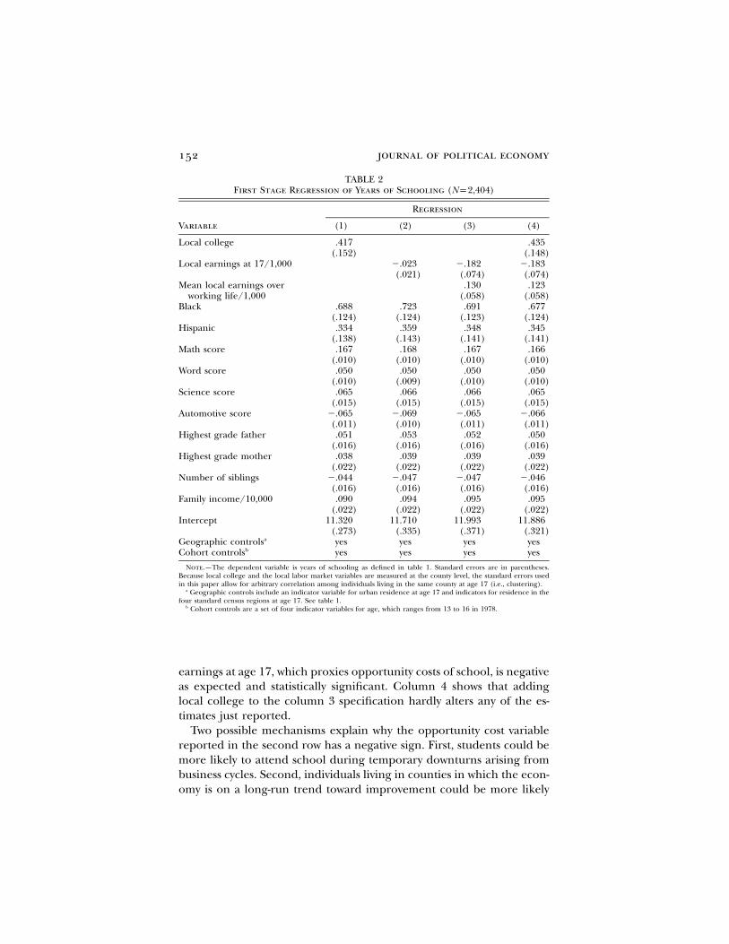
This subsection presents first-stage estimates to demonstrate that theinstruments have predictive power in the first stage and that their signsare consistent with the model presented above. Because individuals ap-pear in our data only after leaving school, the variable measuring school-ing attainment is constant. This makes for difficult interpretation of afirst-stage panel regression of schooling on time-varying local labor mar-ket variables and other characteristics. However, to convey the contentof the first-stage regressions, we construct the variable mean local earn-ings over working life, which takes the mean value of over the yearsl it
in which the individual is included in the wage regressions. We regressschooling on this variable, local earnings at age 17, an indicator for thepresence of a college in the county (local college), and a number ofother control variables.
The first row in column 1 of table 2 shows that local college has alarge and statistically significant effect, implying that individuals with acollege in their county complete almost one-half year more of school,on average. The other covariates have estimates with signs and mag-nitudes consistent with those reported in other work (see, e.g., Cameronand Heckman 2001).
Column 2 reports estimates when local earnings at age 17 is includedin the regression instead of local college (row 2). The estimated coef-ficient has the expected negative sign but is not statistically significantat conventional levels. This variable apparently reflects both time-seriesvariation in county earnings due to business cycle effects and cross-sectional differences in average earnings and wealth across counties.Adding mean local earnings over working life to control for levels ofwealth across counties allows us to sort out these two avenues of influ-ence. The third row of column 3 shows that the coefficient on the newvariable is significant and positive, indicating that students from wealth-ier counties are more likely to attend college—perhaps as a result ofsuperior schools or peer effects. In addition, the coefficient on local
152 journal of political economy
TABLE 2First Stage Regression of Years of Schooling (Np2,404)
Variable
Regression
(1) (2) (3) (4)
Local college .417(.152)
.435(.148)
Local earnings at 17/1,000 �.023(.021)
�.182(.074)
�.183(.074)
Mean local earnings overworking life/1,000
.130(.058)
.123(.058)
Black .688(.124)
.723(.124)
.691(.123)
.677(.124)
Hispanic .334(.138)
.359(.143)
.348(.141)
.345(.141)
Math score .167(.010)
.168(.010)
.167(.010)
.166(.010)
Word score .050(.010)
.050(.009)
.050(.010)
.050(.010)
Science score .065(.015)
.066(.015)
.066(.015)
.065(.015)
Automotive score �.065(.011)
�.069(.010)
�.065(.011)
�.066(.011)
Highest grade father .051(.016)
.053(.016)
.052(.016)
.050(.016)
Highest grade mother .038(.022)
.039(.022)
.039(.022)
.039(.022)
Number of siblings �.044(.016)
�.047(.016)
�.047(.016)
�.046(.016)
Family income/10,000 .090(.022)
.094(.022)
.095(.022)
.095(.022)
Intercept 11.320(.273)
11.710(.335)
11.993(.371)
11.886(.321)
Geographic controlsa yes yes yes yesCohort controlsb yes yes yes yes
Note.—The dependent variable is years of schooling as defined in table 1. Standard errors are in parentheses.Because local college and the local labor market variables are measured at the county level, the standard errors usedin this paper allow for arbitrary correlation among individuals living in the same county at age 17 (i.e., clustering).
a Geographic controls include an indicator variable for urban residence at age 17 and indicators for residence in thefour standard census regions at age 17. See table 1.
b Cohort controls are a set of four indicator variables for age, which ranges from 13 to 16 in 1978.
earnings at age 17, which proxies opportunity costs of school, is negativeas expected and statistically significant. Column 4 shows that addinglocal college to the column 3 specification hardly alters any of the es-timates just reported.
Two possible mechanisms explain why the opportunity cost variablereported in the second row has a negative sign. First, students could bemore likely to attend school during temporary downturns arising frombusiness cycles. Second, individuals living in counties in which the econ-omy is on a long-run trend toward improvement could be more likely
educational borrowing constraints 153
to attend college. In practice, both avenues seem to have influence.21
From the point of view of the theory, the distinction is irrelevant. Whatis important is the comparison of economic conditions during a stu-dent’s college years and conditions later in life. However, the businesscycle influence is more intuitively appealing as a source of identificationsince it does not depend on long-run features of the county of residence,which may be correlated with individual ability outcomes. Unfortunately,we cannot separate out these different sources without losing substantialstatistical power. Evidence reported in Section VE suggests that corre-lation between ability and location may not be an important concern.We show that the time-varying local labor market variable is unrelatedto observed measures of ability, so it seems plausible that labor marketconditions at age 17 are not related to unobserved ability differenceseither.
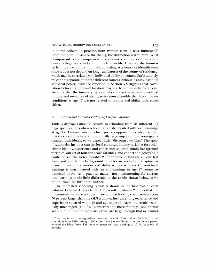
C. Instrumental Variables Excluding Forgone Earnings
Table 3 displays estimated returns to schooling from six different logwage specifications when schooling is instrumented with local earningsat age 17. This instrument, which proxies opportunity costs of school,is not expected to have a differentially large impact on borrowing-con-strained individuals, so we expect little “discount rate bias.” The spec-ification also includes current local earnings, dummy variables for racial-ethnic identity, experience and experience squared, family backgroundvariables, our set of four test score variables, and cohort and geographiccontrols (see the notes to table 2 for variable definitions). Four testscore and four family background variables are included to capture asmany dimensions of unobserved ability as the data allow. Current localearnings is instrumented with current earnings in age 17 county asdiscussed above. As a practical matter, not instrumenting for currentlocal earnings made little difference to the results shown below, so wedo not dwell on this point further.
The estimated schooling return is shown in the first row of eachcolumn. Column 1 reports the OLS results. Column 2 shows that theinstrumental variable point estimate of the schooling coefficient is about50 percent larger than the OLS estimate. Instrumenting experience andexperience squared with age and age squared leaves the results essen-tially unchanged (col. 3). In interpreting these findings, one shouldkeep in mind that the standard errors are large enough that we cannot
21 We reestimated the regressions presented in table 2 controlling for labor marketconditions from 1970 through 1996 rather than just conditions from the time a personentered the labor force. The point estimates on local earnings at 17 fell by about 33percent.
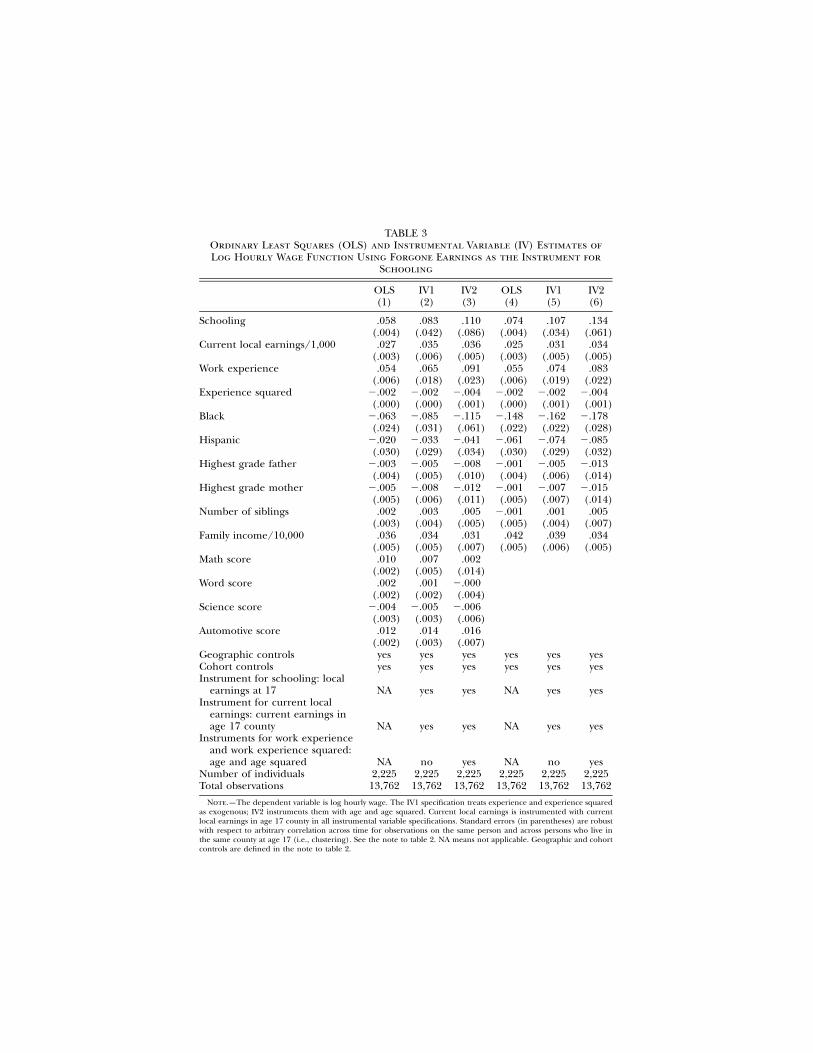
TABLE 3Ordinary Least Squares (OLS) and Instrumental Variable (IV) Estimates ofLog Hourly Wage Function Using Forgone Earnings as the Instrument for
Schooling
OLS(1)
IV1(2)
IV2(3)
OLS(4)
IV1(5)
IV2(6)
Schooling .058(.004)
.083(.042)
.110(.086)
.074(.004)
.107(.034)
.134(.061)
Current local earnings/1,000 .027(.003)
.035(.006)
.036(.005)
.025(.003)
.031(.005)
.034(.005)
Work experience .054(.006)
.065(.018)
.091(.023)
.055(.006)
.074(.019)
.083(.022)
Experience squared �.002(.000)
�.002(.000)
�.004(.001)
�.002(.000)
�.002(.001)
�.004(.001)
Black �.063(.024)
�.085(.031)
�.115(.061)
�.148(.022)
�.162(.022)
�.178(.028)
Hispanic �.020(.030)
�.033(.029)
�.041(.034)
�.061(.030)
�.074(.029)
�.085(.032)
Highest grade father �.003(.004)
�.005(.005)
�.008(.010)
�.001(.004)
�.005(.006)
�.013(.014)
Highest grade mother �.005(.005)
�.008(.006)
�.012(.011)
�.001(.005)
�.007(.007)
�.015(.014)
Number of siblings .002(.003)
.003(.004)
.005(.005)
�.001(.005)
.001(.004)
.005(.007)
Family income/10,000 .036(.005)
.034(.005)
.031(.007)
.042(.005)
.039(.006)
.034(.005)
Math score .010(.002)
.007(.005)
.002(.014)
Word score .002(.002)
.001(.002)
�.000(.004)
Science score �.004(.003)
�.005(.003)
�.006(.006)
Automotive score .012(.002)
.014(.003)
.016(.007)
Geographic controls yes yes yes yes yes yesCohort controls yes yes yes yes yes yesInstrument for schooling: local
earnings at 17 NA yes yes NA yes yesInstrument for current local
earnings: current earnings inage 17 county NA yes yes NA yes yes
Instruments for work experienceand work experience squared:age and age squared NA no yes NA no yes
Number of individuals 2,225 2,225 2,225 2,225 2,225 2,225Total observations 13,762 13,762 13,762 13,762 13,762 13,762
Note.—The dependent variable is log hourly wage. The IV1 specification treats experience and experience squaredas exogenous; IV2 instruments them with age and age squared. Current local earnings is instrumented with currentlocal earnings in age 17 county in all instrumental variable specifications. Standard errors (in parentheses) are robustwith respect to arbitrary correlation across time for observations on the same person and across persons who live inthe same county at age 17 (i.e., clustering). See the note to table 2. NA means not applicable. Geographic and cohortcontrols are defined in the note to table 2.
educational borrowing constraints 155
reject the hypothesis that OLS estimates and instrumental variable es-timates are the same.
Columns 4–6 exhibit estimates of the same specifications except thattest scores and family income are excluded. The OLS and instrumentalvariable point estimates of the schooling coefficient are both higher,but the instrumental variable estimate remains larger than its OLS coun-terpart. Other specifications not reported here, including a more stan-dard one with AFQT score instead of the set of four test scores, all yieldsimilar patterns. These results are also similar to those of Arkes (1998),who uses state unemployment rates in a similar design and finds in-strumental variable estimates higher than OLS estimates.
A potential problem with this specification is that it does not accountfor influences of economic downturns on schooling choices that operatethrough family income or through the decision to work while in college.Borrowing-constrained families may find raising funds for college moredifficult during recessions. This possibility can reverse the direction oflabor market effects: schooling may increase during booms for childrenwhose parents are borrowing-constrained. Thus the influence of locallabor market conditions on schooling attendance is no longer mono-tonic. Intuitively, the income and substitution effects of changes in locallabor market conditions go in opposite directions for borrowing-con-strained families, and it is not clear which effect dominates. However,if families are not borrowing-constrained, there is no income effect onschooling (as in a standard human capital model). Thus it is possiblethat borrowing-constrained families send their children to college athigher rates during a boom, whereas non-borrowing-constrained fam-ilies send their children at higher rates during a bust when forgoneearnings are low.
The negative association between county earnings and schooling re-ported in table 2 supports the dominance of forgone earnings on school-ing decisions. However, this makes the instrumental variable results intable 3 even more surprising. If children of borrowing-constrained fam-ilies have higher marginal returns to schooling and decrease schoolingduring recessions, the discount rate bias should be negative. Our em-pirical findings are counterintuitive if credit constraints are important.The mechanics of this argument are formalized in section A of ourtechnical appendix (available at http://www.econ.northwestern.edu/faculty/taber).
The case in which students work while in school is analogous. Studentswho are borrowing-constrained would presumably be more likely to workin college. Thus the effect of local labor market conditions would likelyhave a larger effect on individuals who are not borrowing-constrainedsince they depend less on opportunities to work during college in order
156 journal of political economy
to attend. Once again, this argument makes the empirical results moresurprising.
D. Instrumental Variables Excluding Direct Costs of Schooling
Estimates of analogous specifications using presence of a local collegeas the instrument for schooling are presented in panel A of table 4.Columns 1–3 present results with no controls for current local earningsin the regression. The OLS results are shown in column 1, instrumentalvariable results in column 2, and instrumental variable results from aspecification that includes instruments for work experience and itssquare appear in column 3. The estimated schooling effect is reportedin the first row of the table. The instrumental variable specifications incolumns 2 and 3 reveal a large, causal effect of schooling: over 300percent larger than the OLS point estimate.
The use of this instrument leads to a concern that colleges are notrandomly assigned to counties in the United States. Thus it makes senseto control for county-level earnings directly in the specification andinstrument for this variable with current earnings in age 17 county,following our discussion above regarding possible endogeneity of thisvariable. Essentially, this addition to the specification controls for dif-ferences in wealth among counties. To our knowledge, this strategy hasnot been tried in other studies that instrument schooling with a variablefor local college access (see the survey in Card [1999]). This controlturns out to be important. Adding current local earnings yields a strik-ingly different pattern: instrumental variable and OLS estimates arenearly identical (cols. 4–6).
Panel B of table 4 confirms these findings using the same specifica-tions reported in panel A with the exception that the AFQT score re-places the four test scores as a control for ability in columns 1–3 andcontrols for ability are dropped altogether for the results shown incolumns 4–6. These specifications are included since they correspondclosely to those commonly found in the literature. The OLS results areshown with AFQT score in column 1 and with no ability measure incolumn 3. When schooling and current local earnings are instrumentedtogether (cols. 2 and 5) and when schooling, current local earnings,experience, and experience squared are all instrumented (cols. 3 and6), the main finding is stronger than suggested by panel A: Instrumentalvariable estimates of the schooling coefficient are well below their OLScounterparts.
This subsection contrasts instrumental variable estimates using directcosts (table 3) with instrumental variable estimates using opportunitycosts (table 4). Theory predicts that if borrowing constraints are im-portant for schooling decisions, instrumental variable estimates using
educational borrowing constraints 157
direct costs will be higher than instrumental variable estimates usingopportunity costs. The results in these tables do not bear out that pre-diction. We find no evidence for discount rate bias using this approach.
E. Validity of the Instruments
In general, without a maintained assumption that one of the instrumentsis valid, it is impossible to test the validity of any of them. In addition,since the causal effect of schooling is assumed to vary across individuals,standard overidentification tests do not apply. Nevertheless, it is stillworthwhile to investigate concerns about correlation between instru-ments and the omitted ability component of wage equation residuals.Finding no relationship between observable measures of ability and theinstruments cannot prove the validity of the instruments since corre-lation with unobserved ability components may remain. Nevertheless,such a finding still lends credence to their use.
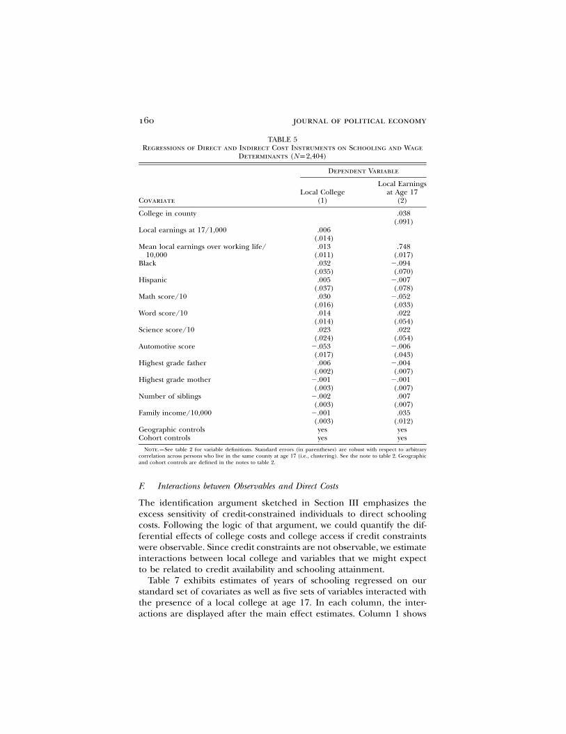
Column 1 of table 5 shows the estimated relationship between theindicator variable for presence of a local college and a standard set ofregressors: local earnings at 17, mean local earnings over the workinglife, racial-ethnic indicators, the set of four test scores, and four familybackground variables. The pattern of estimates is not encouraging forthe use of the local college variable as an instrument: math score andautomotive core are significantly related to presence of a college in thecounty. If local college were correlated with unobserved ability in thesame way as these observed measures, then instrumental variable school-ing estimates would be biased upward.22 Nevertheless, this correlationmakes the instrumental variable results presented above even more sur-prising since it implies that the instrumental variable estimates shouldbe lower than they actually are.
By contrast, the fact that test scores do not predict local earnings atage 17 (col. 2) supports using local labor market variation as an instru-ment. Column 2 also shows that the only variable other than mean localearnings over the working life with any significance is family income.Given that family income is measured when students were close to age17, this result is not particularly astounding.23
The discovery that test scores predict presence of a local college isnot necessarily a problem since test score variables are included in thespecifications. Table 6 displays results that are more favorable to thelegitimacy of using local college as an instrument. The table displays
22 Altonji, Elder, and Taber (2002) provide a model that formally justifies this type ofargument. We do not have enough control variables in this case to use the type of formalanalysis they suggest.
23 Along the same lines, one may question whether family income is a valid control. Theempirical results here are robust to inclusion of family income.
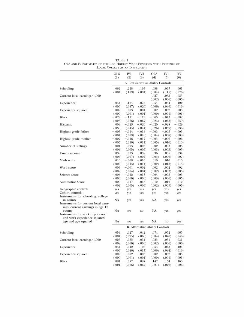
TABLE 4OLS and IV Estimates of the Log Hourly Wage Function with Presence of
Local College as an Instrument
OLS(1)
IV1(2)
IV2(3)
OLS(4)
IV1(5)
IV2(6)
A. Test Scores as Ability Controls
Schooling .062(.004)
.228(.109)
.193(.084)
.058(.004)
.057(.115)
.061(.076)
Current local earnings/1,000 .027(.002)
.035(.006)
.035(.005)
Experience .054(.006)
.124(.047)
.075(.020)
.054(.006)
.054(.049)
.102(.019)
Experience squared �.002(.000)
�.003(.001)
�.004(.001)
�.002(.000)
�.002(.001)
�.005(.001)
Black �.029(.026)
�.111(.066)
�.119(.067)
�.063(.023)
�.073(.063)
�.082(.059)
Hispanic .009(.035)
�.023(.045)
�.020(.044)
�.020(.026)
�.028(.037)
�.029(.036)
Highest grade father �.003(.004)
�.014(.009)
�.015(.010)
�.003(.004)
�.003(.008)
�.003(.008)
Highest grade mother �.002(.005)
�.016(.010)
�.017(.011)
�.005(.005)
�.006(.010)
�.006(.010)
Number of siblings �.001(.004)
.003(.005)
.005(.005)
.002(.003)
.003(.005)
.003(.005)
Family income .039(.005)
.033(.007)
.032(.007)
.036(.005)
.035(.006)
.034(.007)
Math score .010(.002)
�.008(.013)
�.010(.014)
.010(.002)
.010(.013)
.010(.013)
Word score .003(.002)
�.001(.004)
�.002(.004)
.002(.002)
.002(.003)
.002(.003)
Science score �.005(.003)
�.012(.006)
�.013(.006)
�.004(.003)
�.003(.006)
�.003(.005)
Automotive Score .009(.002)
.017(.005)
.018(.006)
.012(.002)
.012(.005)
.012(.005)
Geographic controls yes yes yes yes yes yesCohort controls yes yes yes yes yes yesInstruments for schooling: college
in county NA yes yes NA yes yesInstruments for current local earn-
ings: current earnings in age 17county NA no no NA yes yes
Instruments for work experienceand work experience squared:age and age squared NA no yes NA no yes
B. Alternative Ability Controls
Schooling .054(.004)
.027(.095)
.042(.060)
.074(.004)
.052(.078)
.065(.046)
Current local earnings/1,000 .026(.002)
.035(.006)
.034(.006)
.025(.002)
.031(.006)
.031(.006)
Experience .054(.006)
.042(.046)
.106(.017)
.055(.006)
.043(.044)
.104(.016)
Experience squared �.002(.000)
�.002(.001)
�.005(.001)
�.002(.000)
�.002(.001)
�.005(.001)
Black �.081(.021)
�.077(.066)
�.087(.062)
�.147(.021)
�.154(.026)
�.160(.026)
educational borrowing constraints 159
TABLE 4(Continued)
OLS(1)
IV1(2)
IV2(3)
OLS(4)
IV1(5)
IV2(6)
Hispanic �.040(.026)
�.043(.040)
�.043(.040)
�.061(.026)
�.065(.032)
�.064(.033)
Highest grade father �.004(.004)
�.002(.009)
�.001(.009)
�.001(.004)
.001(.010)
.002(.010)
Highest grade mother �.006(.005)
�.005(.008)
�.005(.008)
�.001(.005)
.001(.011)
.000(.010)
Number of siblings .002(.003)
.003(.004)
.003(.004)
�.001(.003)
�.001(.006)
�.001(.006)
Family income/10,000 .036(.005)
.036(.006)
.036(.006)
.042(.005)
.044(.009)
.043(.009)
AFQT score .005(.001)
.006(.004)
.006(.003)
Geographic controls yes yes yes yes yes yesCohort controls yes yes yes yes yes yesInstrument for schooling: local
college NA yes yes NA yes yesInstrument for current local earn-
ings: current earnings in age 17county NA yes yes NA yes yes
Instruments for work experienceand work experience squared:age and age squared NA no yes NA no yes
Number of individuals 2,225 2,225 2,225 2,225 2,225 2,225Total wage observations 13,762 13,762 13,762 13,762 13,762 13,762
Note.—The dependent variable is log hourly wage. The IV1 specification treats experience and experience squaredas exogenous; IV2 instruments them with age and age squared. Current local earnings is instrumented with currentlocal earnings in age 17 county in cols. 4–6. Standard errors (in parentheses) are robust with respect to arbitrarycorrelation across time for observations on the same person and across persons who live in the same county at age 17(i.e., clustering). Geographic and cohort controls are defined in the notes to table 2. NA means not applicable.
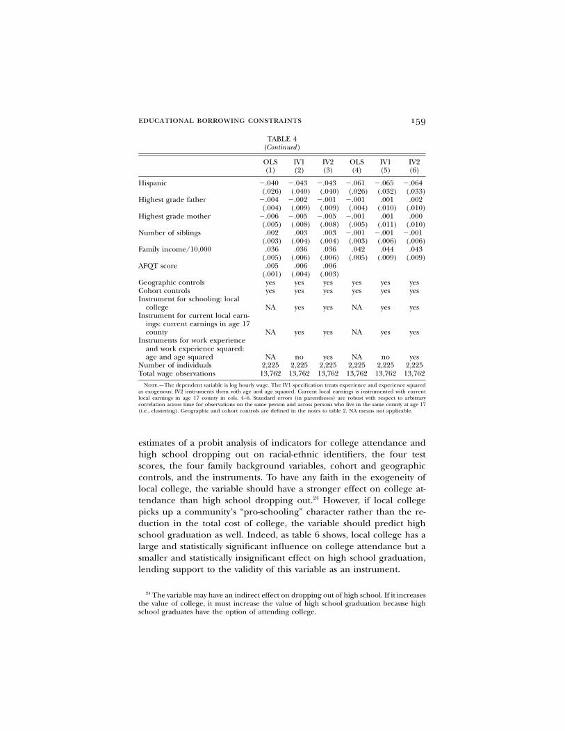
estimates of a probit analysis of indicators for college attendance andhigh school dropping out on racial-ethnic identifiers, the four testscores, the four family background variables, cohort and geographiccontrols, and the instruments. To have any faith in the exogeneity oflocal college, the variable should have a stronger effect on college at-tendance than high school dropping out.24 However, if local collegepicks up a community’s “pro-schooling” character rather than the re-duction in the total cost of college, the variable should predict highschool graduation as well. Indeed, as table 6 shows, local college has alarge and statistically significant influence on college attendance but asmaller and statistically insignificant effect on high school graduation,lending support to the validity of this variable as an instrument.
24 The variable may have an indirect effect on dropping out of high school. If it increasesthe value of college, it must increase the value of high school graduation because highschool graduates have the option of attending college.
160 journal of political economy
TABLE 5Regressions of Direct and Indirect Cost Instruments on Schooling and Wage
Determinants (Np2,404)
Covariate
Dependent Variable
Local College(1)
Local Earningsat Age 17
(2)
College in county .038(.091)
Local earnings at 17/1,000 .006(.014)
Mean local earnings over working life/10,000
.013(.011)
.748(.017)
Black .032(.035)
�.094(.070)
Hispanic .005(.037)
�.007(.078)
Math score/10 .030(.016)
�.052(.033)
Word score/10 .014(.014)
.022(.054)
Science score/10 .023(.024)
.022(.054)
Automotive score �.053(.017)
�.006(.043)
Highest grade father .006(.002)
�.004(.007)
Highest grade mother �.001(.003)
�.001(.007)
Number of siblings �.002(.003)
.007(.007)
Family income/10,000 �.001(.003)
.035(.012)
Geographic controls yes yesCohort controls yes yes
Note.—See table 2 for variable definitions. Standard errors (in parentheses) are robust with respect to arbitrarycorrelation across persons who live in the same county at age 17 (i.e., clustering). See the note to table 2. Geographicand cohort controls are defined in the notes to table 2.
F. Interactions between Observables and Direct Costs
The identification argument sketched in Section III emphasizes theexcess sensitivity of credit-constrained individuals to direct schoolingcosts. Following the logic of that argument, we could quantify the dif-ferential effects of college costs and college access if credit constraintswere observable. Since credit constraints are not observable, we estimateinteractions between local college and variables that we might expectto be related to credit availability and schooling attainment.
Table 7 exhibits estimates of years of schooling regressed on ourstandard set of covariates as well as five sets of variables interacted withthe presence of a local college at age 17. In each column, the inter-actions are displayed after the main effect estimates. Column 1 shows
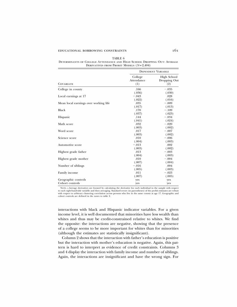
educational borrowing constraints 161
TABLE 6Determinants of College Attendance and High School Dropping Out: Average
Derivatives from Probit Models (Np2,404)
Covariate
Dependent Variable
CollegeAttendance
(1)
High SchoolDropping Out
(2)
College in county .166(.036)
�.035(.030)
Local earnings at 17 �.043(.022)
.028(.016)
Mean local earnings over working life .035(.017)
�.009(.013)
Black .170(.037)
�.109(.023)
Hispanic .144(.041)
�.034(.024)
Math score .032(.003)
�.020(.002)
Word score .017(.003)
�.007(.002)
Science score .010(.004)
�.006(.003)
Automotive score �.013(.003)
.002(.002)
Highest grade father .013(.004)
�.003(.003)
Highest grade mother .010(.007)
�.004(.004)
Number of siblings �.016(.005)
.004(.003)
Family income .011(.007)
�.023(.005)
Geographic controls yes yesCohort controls yes yes
Note.—Average derivatives are formed by calculating the derivative for each individual in the sample with respectto each right-hand-side variable and then averaging. Standard errors (in parentheses) of the probit estimates are robustwith respect to arbitrary clustering correlation across persons who live in the same county at age 17. Geographic andcohort controls are defined in the notes to table 2.
interactions with black and Hispanic indicator variables. For a givenincome level, it is well documented that minorities have less wealth thanwhites and thus may be credit-constrained relative to whites. We findthe opposite: the interactions are negative, showing that the presenceof a college seems to be more important for whites than for minorities(although the estimates are statistically insignificant).
Column 2 shows that the interaction with father’s education is positivebut the interaction with mother’s education is negative. Again, this pat-tern is hard to interpret as evidence of credit constraints. Columns 3and 4 display the interaction with family income and number of siblings.Again, the interactions are insignificant and have the wrong sign. For
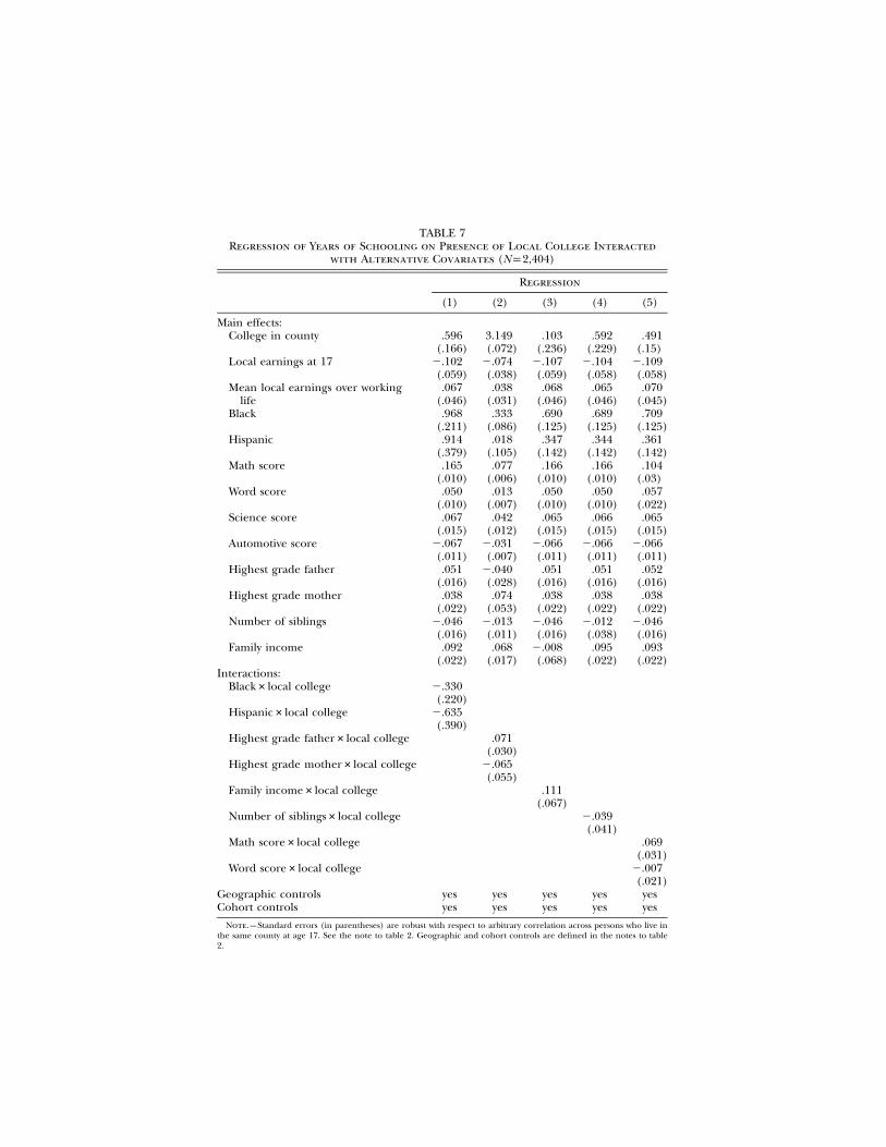
TABLE 7Regression of Years of Schooling on Presence of Local College Interacted
with Alternative Covariates (Np2,404)
Regression
(1) (2) (3) (4) (5)
Main effects:College in county .596
(.166)3.149(.072)
.103(.236)
.592(.229)
.491(.15)
Local earnings at 17 �.102(.059)
�.074(.038)
�.107(.059)
�.104(.058)
�.109(.058)
Mean local earnings over workinglife
.067(.046)
.038(.031)
.068(.046)
.065(.046)
.070(.045)
Black .968(.211)
.333(.086)
.690(.125)
.689(.125)
.709(.125)
Hispanic .914(.379)
.018(.105)
.347(.142)
.344(.142)
.361(.142)
Math score .165(.010)
.077(.006)
.166(.010)
.166(.010)
.104(.03)
Word score .050(.010)
.013(.007)
.050(.010)
.050(.010)
.057(.022)
Science score .067(.015)
.042(.012)
.065(.015)
.066(.015)
.065(.015)
Automotive score �.067(.011)
�.031(.007)
�.066(.011)
�.066(.011)
�.066(.011)
Highest grade father .051(.016)
�.040(.028)
.051(.016)
.051(.016)
.052(.016)
Highest grade mother .038(.022)
.074(.053)
.038(.022)
.038(.022)
.038(.022)
Number of siblings �.046(.016)
�.013(.011)
�.046(.016)
�.012(.038)
�.046(.016)
Family income .092(.022)
.068(.017)
�.008(.068)
.095(.022)
.093(.022)
Interactions:Black#local college �.330
(.220)Hispanic#local college �.635
(.390)Highest grade father#local college .071
(.030)Highest grade mother#local college �.065
(.055)Family income#local college .111
(.067)Number of siblings#local college �.039
(.041)Math score#local college .069
(.031)Word score#local college �.007
(.021)Geographic controls yes yes yes yes yesCohort controls yes yes yes yes yes
Note.—Standard errors (in parentheses) are robust with respect to arbitrary correlation across persons who live inthe same county at age 17. See the note to table 2. Geographic and cohort controls are defined in the notes to table2.
educational borrowing constraints 163
completeness, column 5 presents interactions with math score and wordscore.25 This exercise produces no evidence of credit constraints.
In related work, both Card (1995b) and Kling (2001) examine similarsets of interactions in the National Longitudinal Survey of Young Men(NLS Young Men). They find evidence that individuals from low familybackgrounds are affected more by the presence of a college. Kling alsocompares estimates of interactions on NLSY data and finds the NLSYestimates to be smaller in magnitude and not statistically significantcompared to estimates from NLS Young Men. He reaches essentiallythe same conclusion that we do.
A number of factors may explain why the NLSY results differ fromthose using the NLS Young Men. Chiefly, the NLSY data are taken frommore recent cohorts. Individuals in Card’s data made their high schoolgraduation and college entry decisions in the decade between the early1960s and early 1970s. During this time, few states had significant studentaid programs, and the major federal student grant and guaranteed loanprograms that were passed into legislation in the mid-1960s were notfunded at significant levels until after 1970.26 Thus it is quite possiblethat earlier generations of young people faced credit access problemsthat later cohorts did not. Of course, the data sets differ in other ways,so further exploration of this hypothesis is an important avenue forfuture research.
VI. Evidence from the Structural Model
This section presents estimates of a structural version of the modeldeveloped in Section III. A structural approach is valuable for at leastthree reasons. First, extending the empirical specifications to an explicitstructural model contributes a robustness check to the empirical find-ings. While many empirical economists debate the relative merits ofstructural versus reduced-form or instrumental variable methods, fewdispute that the methods typically depend on different identifying as-sumptions. It is reassuring when one obtains the same results fromdifferent approaches.
A second reason for the structural approach is to obtain the benefitsof formal analysis. The model that guided the regression and instru-mental variable analysis could at best suggest patterns of estimates con-
25 The col. 5 interactions are somewhat difficult to interpret. While word score is in-consequential, math score is positive and significant, indicating that the presence of alocal college induces more schooling from higher-ability students. It is unclear how tointerpret this finding. Given the strength of test scores in predicting schooling, it is notsurprising that the interaction is significant, perhaps as a result of functional form re-strictions in the regression.
26 An exception was the National Direct Student Loan program, which originated in1958. However, the program was small and targeted science and engineering students.
164 journal of political economy
sistent with the presence of borrowing constraints. The framework de-veloped in this section provides an explicit definition of borrowingconstraints and shows how they can be nonparametrically identified.27
The clarity of this approach will aid future analysts in further explo-rations of borrowing constraints. For example, the manner in whichunobserved heterogeneity enters the model is explicitly described. Inaddition, this approach advances our understanding of identificationsince the model exemplifies how the same economic idea (the differ-ence between the effects of direct costs and forgone income in our case)can be used for identification in regression, instrumental variable, andstructural models.
A third advantage of a structural model is that it provides estimatedmagnitudes of the parameters of interest. In our case, the model yieldsexplicit estimates of the extent of borrowing constraints rather thanheuristic tests of existence. Thus the estimated model allows us to per-form and interpret policy simulations, such as predicting the impact ofan expansion of programs giving below-market interest rate loans to thechildren of poor families.28
A. The Econometric Model
This subsection extends the economic framework of Section III intotwo formal econometric models. The first mirrors the regression ap-proach presented in Section VF by assuming that credit cost hetero-geneity is governed by characteristics observable to the economist. Thesecond approach assumes that borrowing constraints enter the modelas unobserved heterogeneity. The notation below follows that estab-lished in Section III, with the exception that the subscript i is introducedto enumerate individuals.
If person i chooses schooling level S, his wages at time t are given by
′ ′ ′log (w ) p g � X b � X b � X b � u , (18)Sit S Wi W Lit L Eit E Sit
where represents a random error term that is person-specific anduSit
specific to each schooling level. For convenience, observed right-hand-side exogenous variables are parceled into three vectors: , a vectorXWi
of characteristics that do not vary over time; , time-varying local laborXLit
market measures; and , time-varying measures of work experienceXEit
(experience and experience squared in our empirical implementationbelow). We assume that the are orthogonal to all right-hand-sideuSit
27 The technical appendix formally proves nonparametric identification.28 We do not perform such counterfactuals in this paper because we find no evidence
of borrowing constraints.
educational borrowing constraints 165
variables for all S and t. Schooling effects are captured through the levelshifter, , and the shocks, .g uS Sit
If individual i were to choose schooling level S, his present value ofearnings discounted to the time he leaves school would be
�
t�S ′ ′ ′d exp (g � X b � X b � X b � u ). (19)� S Wi W Lit L Eit E SittpS
As in Section III, we abstract from uncertainty about the shocksand assume that students choose schooling to solve a certainty{u }Sit
equivalence problem, so random variables are replaced with expectedvalues. Let denote future wage expectations for individual i at timeE 0i
0. Then the certainty equivalent present value of earnings net of directcosts dated at the initial period is defined for schooling level S as
�S1 ′ t�S ′ ′I p exp (g � X b ) d exp [X b � E (X b )�Si S Wi W Eit E 0i Lit L( ) {R tpSi
S�1 t1 ′� E (u )] � X b , (20)�0i Sit Ci C( )} Rtp0 i
where represents the individual borrowing rate. Costs of schoolingR i
( in Sec. III) have been parameterized to depend on observablestt
through the index .29′X bCi C
For empirical implementation, we make three simplifying assump-tions. First, we assume that wage equation residuals take the form
u p v � q , (21)Sit Si Sit
where is a time-invariant random effect known to the individual whenvSi
schooling decisions are made but not observed by the econometrician.The component is assumed orthogonal to all time 0 informationqSit
for all t, so . Both components of the error terms are main-E (u ) p v0i Sit Si
tained to be strictly orthogonal to all right-hand-side observables for allS and t, although may be arbitrarily correlated with for any S andv v ′Si S i
.′SSecond, we approximate time 0 expectations of future local labor
market conditions, , by a linear function of local labor market′E (X b )0i Lit L
variables known to individuals when schooling decisions are made. Welet these variables depend on S and denote them by with associatedXLSi
29 For computational convenience, we have assumed that costs depend only on observ-ables. We see no reason why this should bias the findings in either direction.
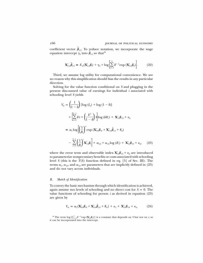
166 journal of political economy
coefficient vector . To reduce notation, we incorporate the wagebLS
equation intercept into so that30˜g bS LS
�
′ ′ t�S ′˜X b { E (X b) � g � log d exp (X b ) . (22)�LSi LS 0i Lit l S Eit E[ ]tpS
Third, we assume log utility for computational convenience. We seeno reason why this simplification should bias the results in any particulardirection.
Solving for the value function conditional on S and plugging in thepresent discounted value of earnings for individual i associated withschooling level S yields
1V p [log (I ) � log (1 � d)]Si Si( )1 � d
S�1 Sdt ′� d t � S log (dR ) � X b � n� i Ti TS Si( )[ ]1 � dtp0
S1 ′ ′ ˜{ a log exp (X b � X b � v )1 Wi W LSi LS Si( )[ R i
S�1 t1 ′ ′� X b � a � a log (R ) � X b � n , (23)� Ci C 2S 3S i Ti TS Si( ) ]Rtp0 i
where the error term and observable index are introduced′X b � nTi TS Si
to parameterize nonpecuniary benefits or costs associated with schoolinglevel S (this is the function defined in eq. [5] of Sec. III). TheT(S)terms , , and are parameters that are implicitly defined in (23)a a a1 2S 3S
and do not vary across individuals.
B. Sketch of Identification
To convey the basic mechanism through which identification is achieved,again assume two levels of schooling and no direct cost for . TheS p 0value functions of schooling for person i as derived in equation (23)are given by
′ ′ ′˜V p a (X b � X b � v ) � a � X b � n (24)0i 1 Wi W L0i L0 0i 1 Ti T 0 0i
30 The term is a constant that depends on S but not on i, so� t�S ′log [� d exp (X b )]Eit EtpS
it can be incorporated into the intercept.
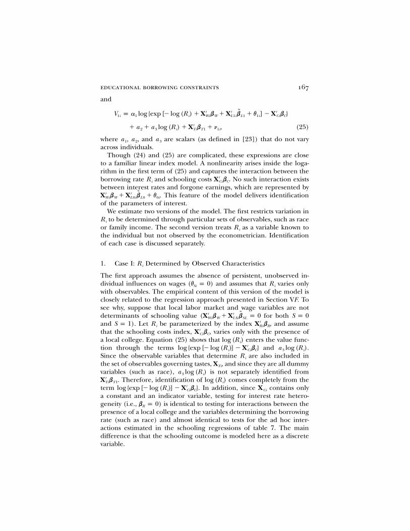
educational borrowing constraints 167
and
′ ′ ′˜V p a log {exp [� log (R ) � X b � X b � v ] � X b }1i 1 i Wi W L1i L1 1i Ci C
′� a � a log (R ) � X b � n , (25)2 3 i Ti T1 1i
where , , and are scalars (as defined in [23]) that do not varya a a1 2 3
across individuals.Though (24) and (25) are complicated, these expressions are close
to a familiar linear index model. A nonlinearity arises inside the loga-rithm in the first term of (25) and captures the interaction between theborrowing rate and schooling costs . No such interaction exists′R X bi Ci C
between interest rates and forgone earnings, which are represented by. This feature of the model delivers identification′ ′ ˜X b � X b � vWi W L0i L0 0i
of the parameters of interest.We estimate two versions of the model. The first restricts variation into be determined through particular sets of observables, such as raceR i
or family income. The second version treats as a variable known toR i
the individual but not observed by the econometrician. Identificationof each case is discussed separately.
1. Case I: Determined by Observed CharacteristicsR i
The first approach assumes the absence of persistent, unobserved in-dividual influences on wages ( ) and assumes that varies onlyv p 0 RSi i
with observables. The empirical content of this version of the model isclosely related to the regression approach presented in Section VF. Tosee why, suppose that local labor market and wage variables are notdeterminants of schooling value ( for both′ ′ ˜X b � X b p 0 S p 0Wi W LSi SL
and ). Let be parameterized by the index , and assume′S p 1 R X bi Ri R
that the schooling costs index, , varies only with the presence of′X bCi C
a local college. Equation (25) shows that enters the value func-log (R )ition through the terms and .′log {exp [� log (R )] � X b } a log (R )i Ci C 3 i
Since the observable variables that determine are also included inR i
the set of observables governing tastes, , and since they are all dummyXTi
variables (such as race), is not separately identified froma log (R )3 i
. Therefore, identification of comes completely from the′X b log (R )Ti T1 i
term . In addition, since contains only′log {exp [� log (R )] � X b } Xi Ci C Ci
a constant and an indicator variable, testing for interest rate hetero-geneity (i.e., ) is identical to testing for interactions between theb p 0R
presence of a local college and the variables determining the borrowingrate (such as race) and almost identical to tests for the ad hoc inter-actions estimated in the schooling regressions of table 7. The maindifference is that the schooling outcome is modeled here as a discretevariable.
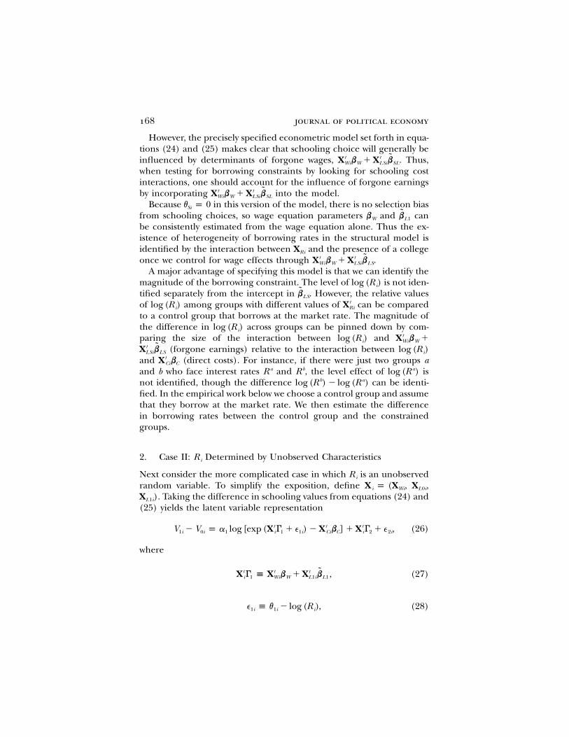
168 journal of political economy
However, the precisely specified econometric model set forth in equa-tions (24) and (25) makes clear that schooling choice will generally beinfluenced by determinants of forgone wages, . Thus,′ ′ ˜X b � X bWi W LSi SL
when testing for borrowing constraints by looking for schooling costinteractions, one should account for the influence of forgone earningsby incorporating into the model.′ ′ ˜X b � X bWi W LSi SL
Because in this version of the model, there is no selection biasv p 0Si
from schooling choices, so wage equation parameters and can˜b bW L1
be consistently estimated from the wage equation alone. Thus the ex-istence of heterogeneity of borrowing rates in the structural model isidentified by the interaction between and the presence of a collegeXRi
once we control for wage effects through .′ ′ ˜X b � X bWi W LSi LS
A major advantage of specifying this model is that we can identify themagnitude of the borrowing constraint. The level of is not iden-log (R )itified separately from the intercept in . However, the relative valuesbLS
of among groups with different values of can be compared′log (R ) Xi Ri
to a control group that borrows at the market rate. The magnitude ofthe difference in across groups can be pinned down by com-log (R )iparing the size of the interaction between and ′log (R ) X b �i Wi W
(forgone earnings) relative to the interaction between′ ˜X b log (R )LSi LS i
and (direct costs). For instance, if there were just two groups a′X bCi C
and b who face interest rates and , the level effect of isa b aR R log (R )not identified, though the difference can be identi-b alog (R ) � log (R )fied. In the empirical work below we choose a control group and assumethat they borrow at the market rate. We then estimate the differencein borrowing rates between the control group and the constrainedgroups.
2. Case II: Determined by Unobserved CharacteristicsR i
Next consider the more complicated case in which is an unobservedR i
random variable. To simplify the exposition, define X p (X , X ,i Wi L0i
. Taking the difference in schooling values from equations (24) andX )L1i
(25) yields the latent variable representation
′ ′ ′V � V p a log [exp (X G � e ) � X b ] � X G � e , (26)1i 0i 1 i 1 1i Ci C i 2 2i
where
′ ′ ′ ˜X G { X b � X b , (27)i 1 Wi W L1i L1
e { v � log (R ), (28)1i 1i i
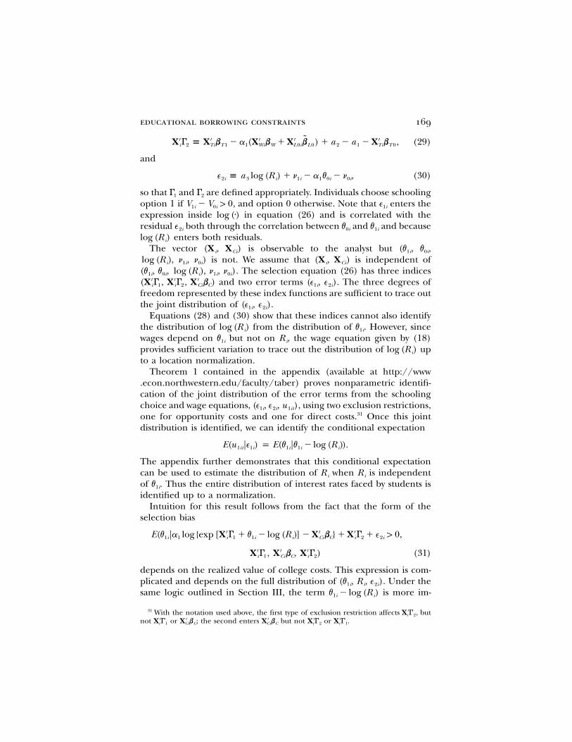
educational borrowing constraints 169
′ ′ ′ ′ ′˜X G { X b � a (X b � X b ) � a � a � X b , (29)i 2 Ti T1 1 Wi W L0i L0 2 1 Ti T 0
and
e { a log (R ) � n � a v � n , (30)2i 3 i 1i 1 0i 0i
so that and are defined appropriately. Individuals choose schoolingG G1 2
option 1 if , and option 0 otherwise. Note that enters theV � V 1 0 e1i 0i 1i
expression inside in equation (26) and is correlated with thelog (7)residual both through the correlation between and and becausee v v2i 0i 1i
enters both residuals.log (R )iThe vector is observable to the analyst but(X , X ) (v , v ,i Ci 1i 0i
is not. We assume that is independent oflog (R ), n , n ) (X , X )i 1i 0i i Ci
. The selection equation (26) has three indices(v , v , log (R ), n , n )1i 0i i 1i 0i
and two error terms . The three degrees of′ ′ ′(X G , X G , X b ) (e , e )i 1 i 2 Ci C 1i 2i
freedom represented by these index functions are sufficient to trace outthe joint distribution of .(e , e )1i 2i
Equations (28) and (30) show that these indices cannot also identifythe distribution of from the distribution of . However, sincelog (R ) vi 1i
wages depend on but not on , the wage equation given by (18)v R1i i
provides sufficient variation to trace out the distribution of uplog (R )ito a location normalization.
Theorem 1 contained in the appendix (available at http://www.econ.northwestern.edu/faculty/taber) proves nonparametric identifi-cation of the joint distribution of the error terms from the schoolingchoice and wage equations, , using two exclusion restrictions,(e , e , u )1i 2i 1it
one for opportunity costs and one for direct costs.31 Once this jointdistribution is identified, we can identify the conditional expectation
E(u Fe ) p E(v Fv � log (R )).1it 1i 1i 1i i
The appendix further demonstrates that this conditional expectationcan be used to estimate the distribution of when is independentR Ri i
of . Thus the entire distribution of interest rates faced by students isv1i
identified up to a normalization.Intuition for this result follows from the fact that the form of the
selection bias′ ′ ′E(v Fa log {exp [X G � v � log (R )] � X b } � X G � e 1 0,1i 1 i 1 1i i Ci C i 2 2i
′ ′ ′X G , X b , X G ) (31)i 1 Ci C i 2
depends on the realized value of college costs. This expression is com-plicated and depends on the full distribution of . Under the(v , R , e )1i i 2i
same logic outlined in Section III, the term is more im-v � log (R )1i i
31 With the notation used above, the first type of exclusion restriction affects , but′X Gi 2
not or ; the second enters but not or .′ ′ ′ ′ ′X G X b X b X G X Gi 1 Ci C Ci C i 2 i 1
170 journal of political economy
portant when costs of schooling are high because the term inlog (7)equation (31) is nonlinear. Suppose that borrowing constraints werenot important. There would be more selection bias in counties that donot have a college since is relatively more important when college isv1i
costly. If borrowing constraints are binding and schooling costs are high,schooling decisions are dictated by borrowing costs. Thus we wouldobserve less selection bias when no college is present.
C. Evidence When Is Determined by Observed CharacteristicsR i
We parameterize interest rates by a function and an index so thatR(7)and , where are observables that govern′R(X b ) ≥ 1 R (0) p 1/d XRi R Ri
the borrowing rate.32 Thus cannot be less than one but can be ar-R i
bitrarily large. This form facilitates comparison between borrowing-con-strained individuals and a control group that is not constrained. Sincewe do not include an intercept in , any population group withX XRi Ri
equal to zero borrows at the market rate. For example, let consistXRi
of dummy variables for black and Hispanic status. For whites, ′X b pRi R
, so . A positive coefficient on the black or Hispanic dummy0 R p 1/di
implies that this subgroup borrows at an interest rate greater than themarket rate.
In this subsection, we report parameter estimates for the model de-fined in equations (18) and (23). To begin, we ignore selection by setting
, which implies that the schooling choice residuals ( ) are in-v p 0 nSi Si
dependent of the wage residuals ( ). This restriction is relaxed in theuSit
next subsection. The parameters are estimated by OLS in a standardbW
Mincer-style log wage regression, and the estimated values are insertedinto the value function (the standard errors of the value function pa-rameters are adjusted appropriately). The cost index, , consists of′X bCi C
only the variable local college and a constant. The vector of taste var-iables, , contains family background variables, AFQT score, minorityXTi
dummies, and dummies for urban residence and region of residence.33
Local labor market variables enter through the index . We in-′ ˜X bLSi LS
corporate two measures of local labor market conditions. The first isthe local earnings variable used above. It is restricted to affect only thewages of high school graduates and high school dropouts. The secondvariable is the long-run average income in the county of residence atage 17 (mean earnings over working life) and affects wages at all school-ing levels.
We allow for four levels of schooling: high school dropout ( ),S p 0
32 The exact form of is .′ ′R(X b ) exp (exp {X b � log [� log (d)]})Ri R Ri R33 Most of these variables entered the schooling regressions in table 2 except the college
in county indicator and the local labor market variables. Also, AFQT is used instead ofthe set of four test scores.
educational borrowing constraints 171
high school graduate ( ), some college ( ), and college grad-S p 2 S p 4uate or more ( ).34 During high school, students incur no directS p 6costs of schooling but must pay some direct costs to attend college andto graduate from college.
We assume that has a generalized extreme value (GEV) distribution,nSi
so the model can be estimated as a nested logit. We use two levels ofnesting. The high school decisions are nested together, and collegedecisions are nested. Observable components of the utilities take theform
′ ′ ˜m p a (X b � X b ) � a ,0i 1 Wi W L0i L0 20
′ ′ ′˜m p a [�2 log (R ) � X b � X b ] � a � a log (R ) � X b ,2i 1 i Wi W L2i L2 22 32 i Ti T 2
34 t1 1′ ′ ′˜m p a log exp (X b � X b ) � X b � a�4i 1 Wi W L4i L4 Ci C 24( ) ( )[ ]R Rtp2i i
′� a log (R ) � X b ,34 i Ti T 4
56 t1 1′ ′ ′˜m p a log exp (X b � X b ) � X b � a�6i 1 Wi W L6i L6 Ci C 26( ) ( )[ ]R Rtp2i i
′� a log (R ) � X b ,36 i Ti T 6
where the are defined in equation (23).ajS
Nesting yields the following schooling probabilities:
exp (m /r )6i cPr (S p 6FS 1 2, m , … , m ) p ,0i 6i exp (m /r ) � exp (m /r )6i c 4i c
Pr (S p 2FS 1 0, m , … , m ) p0i 6i
exp (m /r )2i h ,r /rc hexp (m /r ) � [exp (m /r ) � exp (m /r )]2i h 4i c 6i c
Pr (S p 0Fm , … , m ) p0i 6i
exp (m )0i ,r /r rc h hexp (m ) � {exp (m /r ) � [exp (m /r ) � exp (m /r )] }0i 2i h 4i c 6i c
where and are parameters for the nesting of high school graduatesr rh c
and college attenders, respectively.35 The model is estimated by maxi-mum likelihood, restricting and to lie between zero and one. Taberr rh c
34 Recipients of the general equivalency diploma who attend no college are counted asdropouts (see Cameron and Heckman 1993).
35 The probability for can be constructed from these three probabilities.S p 4
172 journal of political economy
(2000) shows that this nested logit model can be interpreted as a for-ward-looking, discrete-choice dynamic programming model.
A number of normalizations are necessary for identification. We as-sume that for dropouts, which normalizes location as in a stan-b p 0TS
dard polychotomous choice model. In the high school equations, wecannot separately identify the intercepts in from the intercept inbTS
, so the latter are set to zero. We normalize , the coefficient onb bLS C
local college, to one in the equations for college. This normalization isneeded because the scale of the indices cannot be separately distin-guished from the intercept in the tastes index.36
Numerically, we found the intercept in the cost equation to be difficultto nail down, so we fixed it to a value of two in the simulations.37 Ex-tensive experimentation with other values for this parameter showedthat the results were insensitive to this choice. We also had numericaltrouble estimating a precise value for the coefficient on the local earn-ings variable in the college states. A reduced-form regression yielded avalue of approximately 0.3, so we fixed the coefficient to this value inthe two college equations. Again, the results were not sensitive to thisrestriction. Finally, we assumed , which implies a market interestd p 0.97rate of .R p 1/d ≈ 1.031
Table 8 exhibits parameter estimates for the base model, in which wedo not allow for interest rate heterogeneity ( ). Panel A shows′X b p 0Ri R
estimates of taste parameters, panel B shows estimates of local labormarket variables, and panel C shows estimates of the GEV scale andnesting parameters. For the sake of brevity, we do not provide a generaldiscussion of the parameters, but they appear reasonable to us andbroadly consistent with the results in the educational attainment liter-ature discussed in Section IIA.
Column 1 of table 9 exhibits estimated educational borrowing ratesusing four alternative sets of observed characteristics. Column 2 presentsnegative log likelihood values for each specification. Panel B reportsimplied borrowing rates when two indicator variables for black andHispanic racial-ethnic status determine the borrowing rate. Unexpect-edly, point estimates of the borrowing rate come in at the boundaryvalue of 1.0, which implies that blacks and Hispanics borrow for edu-cation below the assumed market interest rate.
Panel C exhibits the case in which borrowing rates depend on parentaleducation through four dummy variables for interactions between fatherand mother with a college education or a high school education. The
36 To see this, notice in eq. (23) that one can multiply by any positive number g,bC
increase the intercept in by , and decrease the intercept in byb log (g) b a log (g)LS TS 1
without changing the value of . Normalizing the scale of in this way performed betterV bSi C
computationally than alternative normalizations.37 This amounts to assuming that living at home cuts the cost of schooling in half.
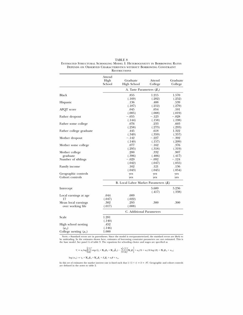
TABLE 8Estimated Structural Schooling Model I: Heterogeneity in Borrowing Rates
Depends on Observed Characteristics without Borrowing ConstraintRestrictions
AttendHigh
SchoolGraduate
High SchoolAttendCollege
GraduateCollege
A. Taste Parameters ( )bT
Black .855(.169)
1.215(.202)
1.570(.252)
Hispanic .136(.187)
.488(.212)
.539(.279)
AFQT score .045(.005)
.054(.008)
.101(.019)
Father dropout �.055(.144)
�.123(.158)
�.028(.198)
Father some college .076(.258)
.233(.273)
.603(.293)
Father college graduate .445(.349)
.618(.359)
1.322(.357)
Mother dropout �.142(.140)
�.227(.157)
�.392(.209)
Mother some college .077(.295)
�.162(.318)
.376(.319)
Mother collegegraduate
.200(.396)
.332(.406)
.907(.417)
Number of siblings �.029(.042)
�.092(.047)
�.124(.055)
Family income .162(.043)
.121(.045)
.136(.054)
Geographic controls yes yes yesCohort controls yes yes yes
B. Local Labor Market Parameters ( )bl
Intercept 5.689(.417)
5.236(.338)
Local earnings at age17
.044(.047)
.009(.022)
Mean local earningsover working life
.302(.017)
.293(.008)
.300 .300
C. Additional Parameters
Scale 1.281(.140)
High school nesting( )rH
.452(.146)
College nesting ( )rC 1.000
Note.—Standard errors are in parentheses. Since the model is overparameterized, the standard errors are likely tobe misleading. In the estimates shown here, estimates of borrowing constraint parameters are not estimated. This isthe base model. See panel A of table 9. The equations for schooling choice and wages are specified as
SS t1 1′ ′ ′ ′˜˜V p a log exp (g � X b � X b ) � X b � a (S) � a (S) log (R ) � X b � u ;�s 1 S Wi W L0i LS Ci C 2 3 i Ti TS TSi( ) ( )[ ]R Rtp0i i
′ ′log (w ) p g � X b � X b � E b � a v � n .Sit S Wi W Lit L it E S Sit
In this set of estimates the market interest rate is fixed such that . Geographic and cohort controls1/(1 � r) p d p .97are defined in the notes to table 2.
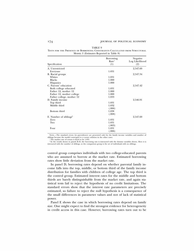
174 journal of political economy
TABLE 9Tests for the Presence of Borrowing Constraints Calculated from Structural
Model I (Estimates Reported in Table 8)
Specification
BorrowingRatea
(1)
NegativeLog Likelihood
(2)
A. Unrestricted 2,547.69Everyone 1.031
B. Racial groups 2,547.34Whites 1.031Blacks 1.000Hispanics 1.000
C. Parents’ education 2,547.42Both college educated 1.031Father 12, mother 12 1.000Father 12, mother college 1.000Father college, mother 12 1.033
D. Family income 2,546.91Top third 1.031Middle third 1.032
(.006)Bottom third 1.038
(.008)E. Number of siblingsb 2,547.69
Zero 1.031Two 1.031
(.003)Four 1.031
(.006)
Note.—The standard errors (in parentheses) are presented only for the family income variables and number ofsiblings because the model converged to a corner solution in the other cases.
a The market rate of return is fixed to be 1.031.b In the results shown in panels B–D, the borrowing rate is interacted with the dummy variables shown. Here it is
interacted with the number of siblings, so the comparison group is the set of individuals with no siblings.
control group comprises individuals with two college-educated parentswho are assumed to borrow at the market rate. Estimated borrowingrates show little deviation from the market rate.
In panel D, borrowing rates depend on whether parental family in-come falls into the top, middle, or bottom third of the family incomedistribution for families with children of college age. The top third isthe control group. Estimated interest rates for the middle and bottomthirds are barely distinguishable from the market rate, and again sta-tistical tests fail to reject the hypothesis of no credit limitations. Thestandard errors show that the interest rate parameters are preciselyestimated, so failure to reject the null hypothesis is a consequence ofthe small differences in parameter values and not of lack of statisticalpower.
Panel E shows the case in which borrowing rates depend on familysize. One might expect to find the strongest evidence for heterogeneityin credit access in this case. However, borrowing rates turn out to be
educational borrowing constraints 175
insensitive to the number of children in the family (number of siblings).Once again, confidence intervals are tight, indicating that the null isrejected because of small coefficients, not lack of power.
D. Evidence When Is Not ObservedR i
Failing to find evidence of heterogeneity in borrowing rates in observ-ables, we extend the structural model to capture borrowing rate het-erogeneity in unobservables. We assume that individuals come in oneof two types: those borrowing at the market rate and those who are1/d
“constrained” and borrow at rate . We estimate the borrowingR 1 1/dc
rate and the fraction of the population that borrows at the higherRc
rate, denoted as . The distribution of borrowing rates is restricted toPc
be independent of the observables and other error terms.Unobserved ability enters the model through a single standard normal
factor , which is known by the agent at the time schooling choices arevi
made and is independent of observables. The error terms in the wageequations are defined as
u p f v � q , (32)Sit WS i Sit
where is the wage equation factor loading term, and is inde-f qWS Sit
pendently and identically distributed over time and is orthogonal tofor all t. Ability may also be correlated with unobserved tastes forvi
schooling. The taste residual for school level S is now defined as
˜n p f v � n , (33)Si TS i Si
where is the tastes equation factor loading for school level S, andfTS
has a GEV distribution, which yields the nested logit model from thenSi
previous section.A major goal of the approach in this subsection is to identify the
extent of borrowing constraints from economic influences regulatingthe behavioral interaction between interest rates and schooling costsand not from functional form assumptions on the distribution of theerror terms. This goal led to two nonstandard estimation strategies. First,because we have no presumption about the form of the selection bias,we retain flexibility in its modeling. Ideally, we would place no restric-tions on the joint distribution of the taste and wage errors (v , v ,2i 4i
. However, full nonparametric estimation of thisv , u , u , u , u )6i 0it 2it 4it 6it
distribution is not computationally feasible. Even after we restrict thedistribution of the error terms to specific functional forms with a one-factor representation, there are still seven factor loading terms on vi
that determine the form of the selection bias. We purposely overparam-eterize the selection bias function in order to force identification from
176 journal of political economy
interactions between the selection terms and the college costs index.As a result, we could not obtain standard errors of the parameters be-cause the estimated Hessian matrix turned out to be approximatelysingular in all cases. This posed little difficulty since consistent esti-mation of the distribution is still possible, and likelihood ratio typeRc
statistics were employed to test for borrowing constraints.We initially attempted to estimate the model using maximum likeli-
hood, but estimates appeared sensitive to restrictions on the factor load-ing terms. In particular, we could not be sufficiently flexible with thedistribution of to distinguish the distribution of from a flexibleq RSi c
functional form for the school choice equation. Identifying the modelthrough stronger functional form restrictions is not in the spirit of ournonparametric identification results. This difficulty led us to a secondnonstandard estimation strategy. We used an iterative procedure to forceidentification of the distribution of and other parameters to comeRc
from appropriate variation in the data.Partition model parameters into those identified primarily from the
selection equation ( ) and those that require the wage equation ( )W W1 2
for identification. Redefine to denote all observables, and letX i
be the log likelihood function for the schooling decisionL(W , W ; X )i 1 2 i
only (derived as a nested logit with unobserved heterogeneity). Themodel is estimated using the following iterative procedure: (1) Fix W2
and solve for the value of that maximizes the log likelihood function.W1
(2) Fix and solve for the value of that minimizes nonlinear leastW W1 2
squares,
N Ti
2{log (w ) � E[log (w )FX , S ; W , W ]} , (34)�� S it S it i i 1 2i iip1 tp1
where represents the realized value of S for person i.Si
We iterate until convergence.38 Locally, this procedure is equivalentto generalized method of moments with moment conditions
�L (W , W ; X )i 1 2 iE p 0,[ ]�W1
�E[log (w )FX , S ; W , W ]S it i i 1 2iE {log (w )S iti[ �W2
� E[log (w )FX , S ; W , W ]} p 0. (35)S it i i 1 2i ]38 In practice we use a damping parameter to aid convergence.
educational borrowing constraints 177
The distribution of was estimated with the parameters in . ToR Wc 2
keep the form of the selection bias flexible, we estimate the factorloading terms on in the wage equation also. We use the followingvi
partition:
˜W p {a , r , r , (b , b : S � {0, 2, 4, 6})},1 1 h c TS LS
cW p {b , b , b , P, R , (g , f , f : S � {0, 2, 4, 6})}.2 W L E c S LS WS
Panel A of table 10 displays parameter estimates from this approach.39
The model produced an estimated borrowing rate of 1.071 for the bor-rowing-constrained group (compared to 1.030 for the unconstrainedgroup). However, the estimate of the fraction of the population bor-rowing at the higher rate hit the boundary constraint so that the esti-mated fraction is essentially zero. Both because of the reason mentionedabove and because the estimate is on the boundary, standard errors ofthe parameters could not be calculated. We experimented with largenumbers of alternative starting values and specifications, none of whichproduced evidence of heterogeneity in borrowing rates. Thus this finalapproach, like the previous ones, provides no evidence that borrowingconstraints are important for schooling decisions.
VII. Summary and Conclusions
This paper develops economic reasoning that shows that direct costs ofschooling affect borrowing-constrained individuals in a fundamentallydifferent way than opportunity costs. Using variation in direct costs andopportunity costs, we test for the importance of educational borrowingconstraints in four different ways: (1) instrumental variable wage re-gressions, (2) years of schooling regressions with interactions betweencollege costs and various observables likely to be correlated with bor-rowing constraints, (3) a structural econometric model in which bor-rowing rates depend on observables, and (4) a structural model thatallows for unobservable heterogeneity in borrowing rates. We find noevidence that borrowing constraints impede schooling progression usingany of the methods.
A cardinal issue that arises with this type of finding is statistical power.Have we found no evidence of borrowing constraints because they are
39 Experimenting with a wide variety of specifications and starting values showed thatthe model did not typically converge when no restrictions were placed on the param-fST
eters (factor loading on heterogeneity in tastes for schooling). Consequently, we restrictedthe factor loadings in the high school dropout and high school graduation equations tobe equal and the some college and graduate college factor loadings to be(f p f )T0 T2
equal also . These restrictions did not appear to affect estimates but aided(f p f )T4 T6
convergence substantially.
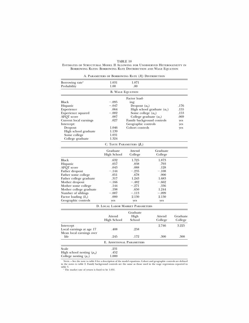
TABLE 10Estimates of Structural Model II Allowing for Unobserved Heterogeneity in
Borrowing Rates: Borrowing Rate Distribution and Wage Equation
A. Parameters of Borrowing Rate ( ) DistributionRi
Borrowing ratea 1.031 1.071Probability 1.00 .00
B. Wage Equation
Black �.095Factor load-
ing:Hispanic �.047 Dropout (a )0 .176Experience .064 High school graduate (a )1 .155Experience squared �.002 Some college (a )2 .153AFQT score .007 College graduate (a )3 .069Current local earnings .027 Family background controls yesIntercept: Geographic controls yes
Dropout 1.046 Cohort controls yesHigh school graduate 1.139Some college 1.031College graduate 1.324
C. Taste Parameters (b )T
GraduateHigh School
AttendCollege
GraduateCollege
Black .632 1.725 1.873Hispanic .057 .838 .793AFQT score .043 .088 .128Father dropout �.144 �.235 �.108Father some college .051 .678 .900Father college graduate .317 1.243 1.683Mother dropout �.166 �.482 �.662Mother some college .144 �.271 .336Mother college graduate .198 .650 1.244Number of siblings �.007 �.113 �.099Factor loading ( )dT .000 2.130 2.130Geographic controls yes yes yes
D. Local Labor Market Parameters
AttendHigh School
GraduateHigh
SchoolAttendCollege
GraduateCollege
Intercept 2.746 3.225Local earnings at age 17 .408 .258Mean local earnings over
life .245 .172 .300 .300
E. Additional Parameters
Scale .231High school nesting ( )rH .452College nesting ( )rC 1.000
Note.—See the note to table 8 for a description of the model equations. Cohort and geographic controls are definedin the notes to table 2. Family background controls are the same as those used in the wage regressions reported intable 3.
a The market rate of return is fixed to be 1.031.
educational borrowing constraints 179
not problematic or because we cannot measure the relevant parameterswith sufficient precision? It is never possible to completely separate thesetwo claims. In the end, the answer chosen depends on prior beliefsabout the size of the effect and the empirical content of the data. Ourview is that power is less of a concern in the schooling choice regressionsand the structural model that restricts borrowing rate heterogeneity tovary with observables. The presence of a local college variable is powerfulin these models; if interactions with it were important, we would expectto detect them. The small standard errors on the interest rates in table9 support this view. Estimates are precise and show little heterogeneityin borrowing rates across families of different sizes and income levels.
By contrast, it is less clear how much power we have with the impre-cisely determined instrumental variable estimates of schooling returns.Nevertheless, in interpreting the instrumental variable results, oneshould keep several points in mind. First, evidence supporting discountrate bias is weak. A number of studies report instrumental variable es-timates of schooling returns larger than OLS estimates, but instrumentalvariable standard errors in these studies are consistently found to belarge. Second, a few recent studies instrument schooling with a variablesuch as presence of a local college. Our results show that these estimatesare sensitive to inclusion of measures for local labor market conditions.Proper inclusion of local labor market controls weakens or eliminatesthe inflated instrumental variable estimates of schooling returns andyields instrumental variable estimates near or below OLS estimates. Itseems plausible that had other researchers included local labor marketcontrols, they may have found instrumental variable estimates of school-ing returns near or below OLS estimates. If so, Card’s (1999) case thatinstrumental variable estimates are consistently higher than OLS esti-mates would weaken considerably. Third, our conclusions are not basedon standard errors alone. Point estimates consistently turn up with thewrong sign to be consistent with credit constraints.
Fourth, theoretical bias arising from problems with instruments inthe instrumental variable wage specifications generally goes in the wrongdirection compared to actual estimates. Table 5 suggests that return toschooling instrumented with presence of a local college may be biasedupward because of potential correlation with unobserved ability. More-over, if family contributions to borrowing-constrained students diminishduring economic recessions, instrumental variable estimates will be bi-ased downward and will come in below OLS estimates. The instrumentalvariable results per se may not be convincing evidence that borrowingconstraints do not exist, but at the very least, they cast doubt on thediscount rate bias story that predicts that instrumental variable estimatesof schooling returns are biased upward.40
40 Ashenfelter, Harmon, and Oosterbeek (1999) have an alternative argument for the
180 journal of political economy
When standard errors could be calculated in the structural selectionmodel, confidence intervals were found to be small. When the param-eters of the heterogeneity distribution converged to boundary values,standard errors could not be calculated. In these cases, though, theboundary values of the estimates imply no heterogeneity in credit access.We believe that this approach is useful and hope that it leads to addi-tional studies.
All told, our results are consistent with the conclusions of Shea (2000),Cameron and Heckman (2001), and Keane and Wolpin (2001). All fourmethods we employ produce no evidence of borrowing constraints.When interpreting our findings, we reiterate two caveats. First, none ofour evidence or the evidence in any of these other studies is direct sincethe actual rates at which individuals borrow for school cannot be ob-served. Second, our results do not imply that credit market constraintswould not exist in the absence of the assortment of private and gov-ernment programs currently available. Instead, our findings show thatgiven the large range of subsidies to education that currently exist, thereis no evidence of underinvestment in schooling resulting from creditaccess.
References
Altonji, Joseph G., and Thomas A. Dunn. 1996. “The Effects of Family Char-acteristics on the Return to Education.” Rev. Econ. and Statis. 78 (November):692–704.
Altonji, Joseph G., Todd E. Elder, and Christopher R. Taber. 2002. “Selectionon Observed and Unobserved Variables: Assessing the Effectiveness of CatholicSchools.” Manuscript. Evanston, Ill.: Northwestern Univ., Dept. Econ.
Angrist, Joshua D., and Alan B. Krueger. 1999. “Empirical Strategies in LaborEconomics.” In Handbook of Labor Economics, vol. 3A, edited by Orley Ashen-felter and David Card. Amsterdam: Elsevier.
Arkes, Jeremy. 1998. “Using State Unemployment Rates during Teenage Yearsas an Instrument to Estimate the Returns to Schooling.” Manuscript. SantaMonica, Calif.: Rand Corp.
Ashenfelter, Orley, Colm Harmon, and Hessel Oosterbeek. 1999. “A Review ofEstimates of the Schooling/Earnings Relationship, with Tests for PublicationBias.” Labour Econ. 6 (November): 453–70.
Becker, Gary S. 1967. Human Capital and the Personal Distribution of Income: AnAnalytical Approach. Woytinsky Lecture no. 1. Ann Arbor, Mich.: Inst. PublicAdmin.
Cameron, Stephen V., and James J. Heckman. 1993. “The Nonequivalence ofHigh School Equivalents.” J. Labor Econ. 11, no. 1, pt. 1 (January): 1–47.
———. 1998. “Life Cycle Schooling and Dynamic Selection Bias: Models andEvidence for Five Cohorts of American Males.” J.P.E. 106 (April): 262–333.
instrumental variable results in the literature. They argue that the pattern may be due toa troubling bias in published specifications. Since instrumental variable standard errorsare often high, if researchers prefer specifications in which the t-statistic is greater thantwo, there will be a bias toward publishing studies with high instrumental variable estimates.
educational borrowing constraints 181
———. 2001. “The Dynamics of Educational Attainment for Black, Hispanic,and White Males.” J.P.E. 109 (June): 455–99.
Card, David. 1995a. “Earnings, Schooling, and Ability Revisited.” In Research inLabor Economics, vol. 14, edited by Solomon W. Polachek. Greenwich, Conn.:JAI.
———. 1995b. “Using Geographic Variation in College Proximity to Estimatethe Return to Schooling.” In Aspects of Labour Market Behaviour: Essays in Honourof John Vanderkamp, edited by Louis N. Christofides, E. Kenneth Grant, andRobert Swidinsky. Toronto: Univ. Toronto Press.
———. 1999. “The Causal Effect of Education on Earnings.” In Handbook ofLabor Economics, vol. 3A, edited by Orley Ashenfelter and David Card. Am-sterdam: Elsevier.
———. 2001. “Estimating the Return to Schooling: Progress on Some PersistentEconometric Problems.” Econometrica 69 (September): 1127–60.
Carneiro, Pedro, James J. Heckman, and Dayanand Manoli. 2002. “Human Cap-ital Policy.” Manuscript. Chicago: Univ. Chicago, Dept. Econ.
Hauser, Robert M. 1993. “Trends in College Entry among Blacks, Whites, andHispanics.” In Studies of Supply and Demand in Higher Education, edited byCharles Clotfelter and Michael Rothschild. Chicago: Univ. Chicago Press (forNBER).
Heckman, James J., and Edward Vytlacil. 1998. “Instrumental Variables Methodsfor the Correlated Random Coefficient Model: Estimating the Average Rateof Return to Schooling When the Return Is Correlated with Schooling.” J.Human Resources 33 (Fall): 974–87.
Imbens, Guido W., and Joshua D. Angrist. 1994. “Identification and Estimationof Local Average Treatment Effects.” Econometrica 62 (March): 467–75.
Kane, Thomas J. 1994. “College Entry by Blacks since 1970: The Role of CollegeCosts, Family Background, and the Returns to Education.” J.P.E. 102 (Octo-ber): 878–911.
Keane, Michael P., and Kenneth I. Wolpin. 2001. “The Effect of Parental Trans-fers and Borrowing Constraints on Educational Attainment.” Internat. Econ.Rev. 42 (November): 1051–1103.
Kling, Jeffrey R. 2001. “Interpreting Instrumental Variables Estimates of theReturns to Schooling.” J. Bus. and Econ. Statis. 19 (July): 358–64.
Lang, Kevin. 1993. “Ability Bias, Discount Rate Bias, and the Return to Educa-tion.” Manuscript. Boston: Boston Univ., Dept. Econ.
Levy, Dan, and Greg Duncan. 2000. “Using Sibling Samples to Assess the Effectof Family Childhood Income on Completed Schooling.” Working Paper no.168 (April). Evanston, Ill.: Northwestern Univ., Joint Center Policy Res.
Lochner, Lance, and Alexander Monge. 2001. “Human Capital Formation withEndogenous Credit Constraints.” Manuscript. Evanston, Ill.: NorthwesternUniv., Dept. Econ.
Manski, Charles F. 1993. “Income and Higher Education.” Focus 14 (Winter):14–19.
Manski, Charles F., and David A. Wise. 1983. College Choice in America. Cambridge,Mass.: Harvard Univ. Press.
Mare, Robert D. 1980. “Social Background and School Continuation Decisions.”J. American Statis. Assoc. 75 (June): 295–305.
Mayer, Susan E. 1997. What Money Can’t Buy: Family Income and Children’s LifeChances. Cambridge, Mass.: Harvard Univ. Press.
Mulligan, Casey B. 1997. Parental Priorities and Economic Inequality. Chicago: Univ.Chicago Press.
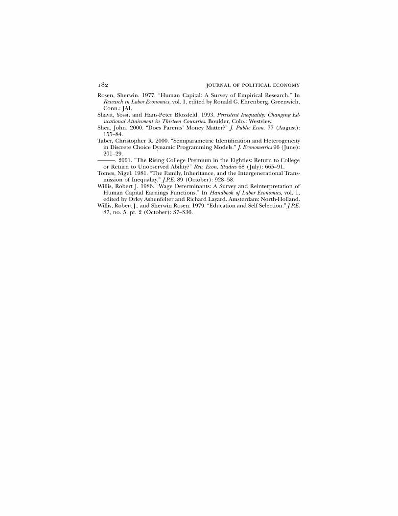
182 journal of political economy
Rosen, Sherwin. 1977. “Human Capital: A Survey of Empirical Research.” InResearch in Labor Economics, vol. 1, edited by Ronald G. Ehrenberg. Greenwich,Conn.: JAI.
Shavit, Yossi, and Hans-Peter Blossfeld. 1993. Persistent Inequality: Changing Ed-ucational Attainment in Thirteen Countries. Boulder, Colo.: Westview.
Shea, John. 2000. “Does Parents’ Money Matter?” J. Public Econ. 77 (August):155–84.
Taber, Christopher R. 2000. “Semiparametric Identification and Heterogeneityin Discrete Choice Dynamic Programming Models.” J. Econometrics 96 (June):201–29.
———. 2001. “The Rising College Premium in the Eighties: Return to Collegeor Return to Unobserved Ability?” Rev. Econ. Studies 68 (July): 665–91.
Tomes, Nigel. 1981. “The Family, Inheritance, and the Intergenerational Trans-mission of Inequality.” J.P.E. 89 (October): 928–58.
Willis, Robert J. 1986. “Wage Determinants: A Survey and Reinterpretation ofHuman Capital Earnings Functions.” In Handbook of Labor Economics, vol. 1,edited by Orley Ashenfelter and Richard Layard. Amsterdam: North-Holland.
Willis, Robert J., and Sherwin Rosen. 1979. “Education and Self-Selection.” J.P.E.87, no. 5, pt. 2 (October): S7–S36.