Estimation of False Discovery Proportion with

Unknown Dependence∗

Jianqing Fan and Xu Han

November 27, 2016

Abstract

Large-scale multiple testing with highly correlated test statistics arises frequently in manyscientific research. Incorporating correlation information in estimating false discovery proportionhas attracted increasing attention in recent years. When the covariance matrix of test statisticsis known, Fan, Han & Gu (2012) provided a consistent estimate of False Discovery Proportion(FDP) under arbitrary dependence structure. However, the covariance matrix is often unknownin many applications and such dependence information has to be estimated before estimatingFDP (Efron, 2010). The estimation accuracy can greatly affect the convergence result of FDPor even violate its consistency. In the current paper, we provide methodological modificationand theoretical investigations for estimation of FDP with unknown covariance. First we developrequirements for estimates of eigenvalues and eigenvectors such that we can obtain a consistentestimate of FDP. Secondly we give conditions on the dependence structures such that the es-timate of FDP is consistent. Such dependence structures include sparse covariance matrices,which have been popularly considered in the contemporary random matrix theory. When dataare sampled from an approximate factor model, which encompasses most practical situations,we provide a consistent estimate of FDP via exploiting this specific dependence structure. Theresults are further demonstrated by simulation studies and some real data applications.

Keywords: Approximate factor model, large-scale multiple testing, dependent test statistics, un-known covariance matrix, false discovery proportion

∗Address Information: Jianqing Fan, Department of Operations Research & Financial Engineering, PrincetonUniversity, Princeton, NJ 08544, USA. Email: jqfan@princeton.edu. This research was partly supported by NIHGrants R01-GM072611 and R01GM100474-01 and NSF Grant DMS-1206464. We would like to thank to Dr. WeijieGu for various assistance on this project.

1

arX

iv:1

305.

7007

v1 [

stat

.ME

] 3

0 M

ay 2

013

1 Introduction

The correlation effect of dependent test statistics in large-scale multiple testing has attracted much

attention in recent years. In microarray experiments, thousands of gene expressions are usually

correlated when cells are treated. Applying standard Benjamini & Hochberg (1995, B-H) or Storey

(2002)’s procedures for independent test statistics can lead to inaccurate false discovery control.

Statisticians have now reached the conclusion that it is important and necessary to incorporate the

dependence information in the multiple testing procedure. See Efron (2007, 2010), Leek & Storey

(2008), Schwartzman & Lin (2011) and Fan, Han & Gu (2012).

Consideration of multiple testing procedure for dependent test statistics dates back to early

2000’s. Benjamini & Yekutieli (2001) proved that the false discovery rate can be controlled by

the B-H procedure when the test statistics satisfy a theoretical dependence structure (positive

regression dependence on subsets, PRDS). Extension to a generalized stepwise multiple testing

procedure under PRDS has been proved by Sarkar (2002). Later Storey, Taylor & Siegmund (2004)

also showed that Storey’s procedure can control FDR under weak dependence. Sun & Cai (2009)

developed a multiple testing procedure where parameters underlying test statistics follow a hidden

Markov model. Insightful results of validation for standard multiple testing procedures under more

general dependence structures have been shown in Clarke & Hall (2009). However, even if the

procedures are valid under these special dependence structures, they still suffer from efficiency loss

without considering the actual dependence information. In other words, there are universal upper

bounds for a given class of covariance matrices.

A challenging question is how to incorporate the correlation effect in the testing procedure. Fan,

Han & Gu (2012) considered the following set-up. Assume the test statistics are from a multivariate

normal distribution with a known covariance matrix. The unknown mean vector is sparse and the

covariance matrix can be arbitrary. The goal is to test each coordinate of the normal mean equals

zero or not. The basic idea of their testing procedure is to apply spectral decomposition to the

covariance matrix of test statistics and use principal factors to account for dependency such that

the remaining dependence is weak. This method is call Principal Factor Approximation (PFA). The

authors provided a consistent estimate of false discovery proportion (FDP) based on the eigenvalues

and eigenvectors of the known covariance matrix.

A major restriction of the setup in Fan, Han & Gu (2012) is that the covariance matrix of

test statistics is known. Although the authors provided an interesting application with known

covariance matrix, in many other cases, the covariance matrix is usually unknown. For example,

in microarray experiments, scientists are interested in testing if genes are differently expressed

under different experimental conditions (e.g. treatments, or groups of patients). The dependence

2

of test statistics is unknown in such applications. Yet, such dependence information is needed for

estimating FDP, and the accuracy of estimated covariance matrix may greatly affect the convergence

result of FDP or even violate its consistency. In the contemporary random matrix theory, it is well

known that the eigenvalues and eigenvectors of the sample covariance matrix are not necessarily

consistent estimates of their corresponding population ones when the sample size is comparable to

or smaller than the dimension. Since PFA critically depends on the eigenvalues and eigenvectors of

estimated covariance matrix, more theoretical justifications and methodological modifications are

needed before directly applying PFA to unknown dependence.

Some recent work has focused on the large-scale multiple testing when the dependence infor-

mation has to be estimated. Efron (2007) in his seminal work obtained repeated test statistics

based on the bootstrap sample from the original raw data, and took out the first eigenvector of

the covariance matrix of the test statistics such that the correlation effect could be explained by a

dispersion variate A. His procedure is then to estimate A from the data and construct an estimate

for realized FDP using A. Following the framework of Leek & Storey (2008), Friguet, Kloareg

& Causeur (2009) and Desai & Storey (2012) assumed that the data come directly from a factor

model with independent idiosyncratic errors, and used the EM algorithms to estimate the number

of factors, the factor loadings and the realized factors in the model and obtained an estimator for

FDP by subtracting out realized common factors. The drawbacks of the aforementioned procedures

are, however, restricted model assumptions and the lack of formal justification.

The current paper provides theoretical investigations for the unknown dependence covariance.

We first develop requirements for estimated eigenvalues and eigenvectors such that a consistent

estimate of FDP can be obtained. Surprisingly, we do not need these estimates of eigenvalues and

eigenvectors to be consistent themselves. This finding relaxes the consistency restriction of covari-

ance matrix estimation under operator norm. We then give regularity conditions on the dependence

structure such that the estimate of FDP is consistent. After that, we study an approximate factor

model for the test statistics. This factor model encompasses a majority of statistical applications

and is a generalization to the model in Friguet, Kloareg & Causeur (2009) and Desai & Storey

(2012), where the random errors can be independent or have sparse dependence. After applying

Principal Orthogonal complEment Thresholding (POET) estimators (Fan, Liao & Mincheva, 2013)

to estimate the unknown covariance matrix, we can develop a consistent estimate of FDP. This

combination of POET to estimate the covariance matrix and PFA to estimate FDP should be appli-

cable to most practical situations and is the method that we recommend for practical applications.

The performance of our procedure is further evaluated by simulation studies and real data analysis.

The organization of the rest of the paper is as follows: Section 2 provides background information

of high dimensional multiple testing under dependency and Principal Factor Approximation (PFA),

3

Section 3 includes the theoretical study on consistency of FDP estimators, Section 4 contains sim-

ulation studies, and Section 5 illustrates the methodology via an application to a microarray data

set. Throughout this paper, we use λmin(A) and λmax(A) to denote the minimum and maximum

eigenvalues of a symmetric matrix A. We also denote the Frobenius norm ‖A‖F = tr1/2(ATA)

and the operator norm ‖A‖ = λ1/2max(ATA). When A is a vector, the operator norm is the same as

the Euclidean norm.

2 Estimation of FDP

Suppose that the observed data Xini=1 are p-dimensional independent random vectors with Xi ∼

Np(µ,Σ). The mean vector µ = (µ1, · · · , µp)T is a high dimensional sparse vector, but we do not

know which ones are the nonvanishing signals. Let p0 = #j : µj = 0 and p1 = #j : µj 6= 0 so

that p0 + p1 = p. The sparsity assumption imposes p1/p → 0 as p → ∞. We wish to test which

coordinates of µ are signals based on the realizations xini=1.

Consider the test statistics Z =√nX in which X is the sample mean of Xini=1. Then, Z ∼

Np(√nµ,Σ). Standardizing the test statistics Z, we assume for simplicity that Σ is a correlation

matrix. Let µ? = (µ?1, · · · , µ?p)T =√nµ. Then, multiple testing

H0j : µj = 0 vs H1j : µj 6= 0

is equivalent to test

H0j : µ?j = 0 vs H1j : µ?j 6= 0

based on the test statistics Z = (Z1, · · · , Zp)T . The P-value for the jth hypothesis is 2Φ(−|Zj |),

where Φ(·) is the cumulative distribution function of the standard normal distribution. We use a

threshold value t to reject the hypotheses which have p-values smaller than t.

Define the number of discoveries R(t) and the number of false discoveries V (t) as

R(t) = #Pj : Pj ≤ t, V (t) = #true null Pj : Pj ≤ t

where Pj is the p-value for testing the jth hypothesis. Our interest focuses on estimating the false

discovery proportion FDP(t) = V (t)/R(t), here and hereafter the convention 0/0 = 0 is always

used. Note that R(t) is observable, but FDP(t) is a realized but unobservable random variable.

4

2.1 Impact of dependence on FDP

To gain the insight on how the dependence of test statistics impacts on the FDP, let us first examine

a simpler problem: The test statistic depends on a common factor

Zi = µ?i + biW + (1− b2i )1/2εi, (1)

where W and εini=1 are independent, having the standard normal distribution. Let zα be the

α-quantile of the standard normal distribution and N = i : µ?i = 0 is the true null set. Then,

V (t) =∑i∈N

I(|Zi| > −zt/2)

=∑i∈N

[I(biW + εi/ai > −zt/2) + I(biW + εi/ai < zt/2)],

where ai = (1− b2i )−1/2. By using the law of large numbers, conditioning on W , under some mild

conditions, we have

V (t) ≈∑i∈N

[Φ(ai(zt/2 + biW )) + Φ(ai(zt/2 − biW ))]. (2)

The dependence of V (t) on the realization W is evidenced in (2). For example, if bi = ρ,

V (t) ≈ p0

[Φ

(zt/2 + ρW√

1− ρ2

)+ Φ

(zt/2 − ρW√

1− ρ2

)]. (3)

When ρ = 0, V (t) ≈ p0t as expected. To quantify the dependence on the realization of W , let

p0 = 1000 and t = 0.01 and ρ = 0.8 so that

V (t) ≈ 1000[Φ((−2.236 + 0.8W )/0.6) + Φ((−2.236− 0.8W )/0.6)].

When W = −3,−2,−1, 0, the values of V (t) are approximately 608, 145, 8 and 0, respectively.

This is in contrast with the independence case in which V (t) is always approximately 10.

Despite the dependence of V (t) on the realized random variable W , the common factor can be

inferred from the observed test statistics. For example, ignoring sparse µ?i in (1), we can estimate

W via the simple least-squares: Minimizing with respect to W

p∑i=1

(Zi − biW )2. (4)

Substituting the estimate into (3) and replace p0 by p, or more generally substituting the estimate

5

into (2) and replace N by the entire set, we obtain an estimate of V (t) under dependence. A robust

implementation is to use L1-regression which finds W to minimize∑p

i=1 |Zi − biW |. This is the

basic idea behind Fan, Han & Gu (2012).

2.2 Principal Factor Approximation

Let λ1, · · · , λp be the eigenvalues of Σ in non-increasing order, and γ1, · · · ,γp be their correspond-

ing eigenvectors. For a given integer k, decompose Σ as

Σ = BBT + A

where B = (√λ1γ1, · · · ,

√λkγk) are unnormalized k principal components and A =

∑pi=k+1 λiγiγ

Ti .

Correspondingly, decompose the test statistics Z ∼ N(µ?,Σ) stochastically as

Z = µ? + BW + K (5)

where W ∼ Nk(0, Ik) are k common factors and K ∼ N(0,A) are the idiosyncratic errors, inde-

pendent of W.

Define the oracle FDP(t) as

FDPoracle(t) =∑

i∈true nulls

[Φ(ai(zt/2 + ηi)) + Φ(ai(zt/2 − ηi))]/R(t)

where ai = (1−‖bi‖2)−1/2, ηi = bTi W and bTi is the ith row of B. This is clear a generalization of

(2). Then, an examination of the proof of Fan, Han & Gu (2012) yields the following result:

Proposition 1. If (C0): p−1√λ2k+1 + · · ·+ λ2p = O(p−δ) for some δ > 0 and (C1) : R(t)/p > H

for some constant H > 0 as p→∞, then |FDPoracle(t)− FDP(t)| = Op(p−δ/2).

Theorem 1 of Fan, Han & Gu (2012) shows that limp→∞[FDPoracle(t)−FDP(t)] = 0 a.s. under

(C0). Here we strengthen the result by presenting the convergence rate p−δ/2. Suppose we choose

k′ > k. Then by (C0) it is easy to see that the associated convergence rate p−δ′/2 is no slower

than p−δ/2. This explains that with more common factors in model (5), FDPoracle(t) converges to

FDP(t) faster as p → ∞. This result will be useful for the discussion about determining number

of factors in section 3.4.

Condition (C0) in Proposition 1 implies that if ‖Σ‖ = o(p1/2), we can take k = 0. In other

words, ‖Σ‖ = o(p1/2) can be regarded as the condition for weak dependence for multiple testing

problem.

6

Since we do not know which coordinates of µ vanish and the set of true nulls is nearly the whole

set, FDPoracle(t) can be well approximated by

FDPA(t) =

p∑i=1

[Φ(ai(zt/2 + ηi)) + Φ(ai(zt/2 − ηi))]/R(t). (6)

Let

FDPA(t) =

p∑i=1

[Φ(ai(zt/2 + ηi)) + Φ(ai(zt/2 − ηi))]/R(t), (7)

where ηi = bTi W for some estimator W of W. Then, under mild conditions, Fan, Han & Gu

(2012) shows ∣∣FDPA(t)− FDPA(t)∣∣ = O(‖W −W‖).

This method is called principal factor approximation (PFA).

For the estimation of W, since µ? is high dimensional sparse, one can consider the following

penalized least-squares estimator based on model (5). Namely, W is obtained by minimizing

p∑i=1

(zi − µ?i − bTi W)2 +

p∑i=1

pλ(|µ?i |) (8)

with respect to µ? and W, where pλ can be the L1 (soft), hard or SCAD penalty function. When

pλ(|µ∗i |) = λ|µ∗i |, the optimization problem in (8) is equivalent to

minW

p∑i=1

ψ(zi − bTi W) (9)

where ψ(·) is the Huber loss function (Fan, Tang & Shi, 2012). In Fan, Han & Gu (2012), they

also considered an alternative loss function for (9), the least absolute deviation loss:

minW

p∑i=1

|zi − bTi W|. (10)

Fan, Tang & Shi (2012) study (8) rigourously, in which the µ?i are called incidental parameters

and W is called common parameters. They show that the penalized estimator of W is consistent

and that its asymptotic distributions are Gaussian. Interestingly, with the sparsity assumption on

the incidental parameters, the penalized estimators of µ?i achieve partial selection consistency,

that is, the large and zero µ?i ’s are correctly estimated as nonzero and zero, but the small µ?i ’s are

incorrectly estimated as zero. Interested readers are referred to Fan, Tang & Shi (2012) for more

theoretical details.

7

2.3 PFA with Unknown Covariance

The estimator FDPA(t) in (7) is based on eigenvalues λiki=1 and eigenvectors γiki=1 of the true

covariance matrix Σ. When Σ is unknown, we need an estimate Σ. Let λ1, · · · , λp be eigenvalues

of Σ in a non-increasing order and γ1, · · · , γp ∈ Rp be their corresponding eigenvectors. One can

obtain an estimator of FDP by substituting unknown eigenvalues and eigenvectors in (7) by their

corresponding estimates. Two questions arise naturally:

(1) What are the requirements for the estimates of λiki=1 and γiki=1 such that a consistent

estimate of FDP(t) can be obtained?

(2) Under what dependence structures of Σ, can such estimates of λiki=1 and γiki=1 be con-

structed?

For question (1), the estimator FDPA(t) is a complicated nonlinear function of λiki=1 and γiki=1.

An appropriate choice of estimates of eigenvalues, eigenvectors and the realized values of common

factors wiki=1 is required. For question (2), it is related to the topics such as random matrix theory

and principal component analysis. The difficulty is to make weak assumptions on the structure of

Σ, which is itself an open question in the above research areas. The current paper will address

these two questions and provide consistent estimate of FDP(t).

3 Main Result

We first present the results for a generic estimator Σ and then focus the covariance matrix estima-

tion for an approximate factor models. All the proofs are relegated to the appendix.

3.1 Required Accuracy

Suppose that (C0) is satisfied for Σ. Let Σ be an estimator of Σ, and correspondingly we have

λiki=1 and γiki=1 to estimate λiki=1 and γiki=1. Analogously, we define B and bi. Note

that we only need to estimate the first k eigenvalues and eigenvectors but not all of them. More

discussions for the case with unknown number of factors are in Section 3.4.

The realized common factors W can be estimated robustly by using (8) and (9) with bi replaced

by bi. To simplify the technical arguments, we here simply use the least-squares estimate

W = (BTB)−1B

TZ, (11)

8

which ignores the µ? in (5) and replaces B by B. Define

FDPU (t) =

p∑i=1

[Φ(ai(zt/2 + ηi)) + Φ(ai(zt/2 − ηi))]/R(t) (12)

where ai = (1 − ‖bi‖2)−1/2 and ηi = bT

i W. Then we can show in Theorem 1 that FDPU (t) is a

consistent estimate of FDPA(t) under some mild conditions.

Theorem 1. Under the following conditions

(C1) R(t)/p > H for H > 0 as p→∞,

(C2) maxi≤k ‖γi − γi‖ = Op(p−κ) for κ > 0,

(C3)∑k

i=1 |λi − λi| = Op(p1−δ) for δ > 0,

(C4) ai ≤ τ1 and ai ≤ τ2 ∀i = 1, · · · , p for some finite constants τ1 and τ2,

we have

|FDPU (t)− FDPA(t)| = Op(p−min(κ,δ)) +Op(kp

−κ) +Op(k‖µ?‖p−1/2).

Using∑k

i=1 λi ≤ tr(Σ) = p, we have∑k

i=1 |λi − λi| ≤ pmaxi≤k |λi/λi − 1|. Thus, Condition

(C3) holds when maxi≤k |λi/λi−1| = Op(p−δ). The latter is particularly relevant when eigenvalues

are spiked. The third term in the convergent result comes really from the least-squares estimate. If

a more sophisticated method such as (8) or (9) is used, the bias will be smaller (Fan, Tang & Shi,

2012). When µ?i pi=1 are truly sparse, it is expected that ‖µ?‖ grows slowly or is even bounded so

that k‖µ?‖p−1/2 → 0 as p → ∞. (C4) is a reasonable condition in practice. It suggests that the

variances of Ki in (5) and their estimates do not converge to zero.

3.2 Results in Eigenvectors and Eigenvalues

Lemma 1. For any matrix Σ, we have

|λi − λi| ≤ ‖Σ−Σ‖ and ‖γi − γi‖ ≤√

2‖Σ−Σ‖min(|λi−1 − λi|, |λi − λi+1|)

.

The first result is referred to Weyl’s Theorem (Horn & Johnson, 1990) and the second result

is called the sin θ Theorem (Davis & Kahan, 1970). They have been applied in sparse covariance

matrix estimation (El Karoui, 2008; Ma, 2013). By Lemma 1, the consistency of eigenvectors and

eigenvalues is directly associated with the operator norm consistency. Several papers have shown

that under various sparsity conditions on Σ, Σ can be constructed such that ‖Σ −Σ‖ → 0. For

9

example, Bickel & Levina (2008) showed that ‖Σ −Σ‖2 = Op(log pn ). In the following Theorem 2,

we will provide consistent estimate of FDP.

Theorem 2. If λi − λi+1 ≥ dp for a sequence dp bounded from below for i = 1, · · · , k, and

‖Σ−Σ‖ = Op(dpp−τ ), and in addition (C1) and (C4) in Theorem 1 are satisfied, then

|FDPU (t)− FDPA(t)| = Op

(kp−τdp/p+ (k + 1)p−τ + k‖µ?‖p−1/2

).

Note that the first k eigenvalues should be distinguished with a certain amount of gap dp. The

theorem is so written that it is applicable to both spike or non-spike case. For the non-spike case,

typically dp = d > 0. In this case, the covariance is estimated consistently and the first term in

Theorem 2 now becomes Op(kp−τ−1

). For the spiked case such as the k-factor model (5), the first

k eigenvalues are of order p and the (k+1)th eigenvalue is of order 1 (Fan, Liao & Mincheva, 2013).

Therefore, dp p. In this case, the covariance matrix can not be consistently estimated, and the

first term is of order O(kp−τ ). See section 3.3 for additional details.

3.3 Approximate Factor Model

In this section, we will study the multiple testing problem where the test statistics have some

strong dependence structure to complement the results in Theorem 2. Assume the dependence of

high-dimensional variable vector of interest can be captured by a few latent factors. This factor

structure model has long history in financial econometrics (Engle & Watson 1981, Bai 2003, Fan,

Liao & Mincheva, 2011). In recent years, strict factor model has received favorable attention in

genomic research (Carvalho, etc 2008, Friguet, Kloareg & Causer 2009, Desai & Storey 2012). Major

restrictions in these models are that the idiosyncratic errors are independent. A more practicable

extension is the approximate factor model (Chamberlain & Rothschild 1983, Fan, Liao & Mincheva,

2011, 2013).

The approximate factor model takes the form

Xi = µ + Bfi + ui, i = 1, · · · , n (13)

for each observation, where µ is a p-dimensional unknown sparse vector, B = (b1, · · · ,bp)T is the

factor loading matrix, fi are common factors to the ith observations, independent of the noise ui ∼

Np(0,Σu) where Σu is sparse. The common factor fi drives the dependence of the measurements

(e.g. gene expressions) within the ith sample. Under model (13), the covariance matrix of Xi is

given by

Σ = Bcov(f)BT + Σu.

10

We can also assume without loss of generality the identifiability condition: cov(f) = IK and the

columns of B are orthogonal. See Fan, Liao & Mincheva (2013).

For the random errors u, let σu,ij be the (i, j)th element of covariance matrix Σu of u. Then

we impose a sparsity condition on Σu:

mp = maxi≤p

∑j≤p|σu,ij |q, mp = o(p) (14)

for some q ∈ [0, 1). It is a standard sparsity condition in Bickel & Levina (2008), Rothman, Levina

& Zhu (2009), Cai & Liu (2012), among others.

Under (13), the test statistics X? =√nX follow the approximate factor model

X? = µ? + Bf? + u? ∼ N(µ?,Σ), (15)

where µ? =√nµ, f? =

√nf and u? =

√nu with f and u being the corresponding mean vector.

Fan, Liao & Mincheva (2013) developed a method called POET to estimate the unknown Σ

based on samples Xini=1 in (13). The basic idea is to take advantage of the factor model structure

and the sparsity of the covariance matrix of idiosyncratic noises. Their idea combined with PFA

in Fan, Han & Gu (2012) yields the following POET-PFA method.

1. Compute sample covariance matrix Σ and decompose Σ =∑p

i=1 λiγiγTi , where λi and γi

are the eigenvalues and eigenvectors of Σ. Apply a thresholding method to∑p

i=k+1 λiγiγTi to

obtain ΣTu (e.g. the adaptive thresholding method in Appendix A). Set ΣPOET =

∑ki=1 λiγiγ

Ti +

ΣTu .

2. Apply singular value decomposition to ΣPOET. Obtain its eigenvalues λ1, · · · , λK in non-

increasing order and the associated eigenvectors γ1, · · · , γK .

3. Construct B = (λ1/21 γ1, · · · , λ

1/2K γK) and compute the least-squares f

?= (B

TB)−1B

T√nX,

which is the least-squares estimate from (15) with µ? ignored.

4. With bT

i denoting the ith row of B, compute

FDPPOET(t) =

p∑i=1

[Φ(ai(zt/2 + bT

i f?)) + Φ(ai(zt/2 − b

T

i f?))]/R(t) (16)

for some threshold value t, where ai = (1− ‖bi‖2)−1/2.

Theoretical results regarding the convergence rates of estimated eigenvalues and eigenvectors

based on POET with adaptive thresholding method are provided in Theorem 3.

11

Theorem 3. Under the conditions of Lemma 2 in Appendix A,

|λi − λi| = Op

(pωp +mpω

1−qp

)where ωp = 1√

p +√

log pn . Then under Assumption 1, we have

‖γi − γi‖ = Op(ωp +mpω1−qp p−1) for 1 ≤ i ≤ k.

Correspondingly, the convergence rate of FDPPOET(t) is as follows:

Theorem 4. Under the conditions in Theorem 3, and in addition (C1) and (C4) in Theorem 1

are satisfied, then

∣∣∣FDPPOET(t)− FDP(t)∣∣∣ = Op

(k(ωp +mpω

1−qp p−1)

)+Op

(k‖µ?‖p−1/2

)+Op

(m1/2p p−1/2 + p1/p

).

3.4 Selecting k

In section 3.1, we assume the number of factors k is known. If the covariance matrix Σ is known,

in practice, we can choose the smallest k such that

p−1√λ2k+1 + · · ·+ λ2p < ε (17)

holds for a predetermined small ε. However, in the current paper setup, Σ is unknown. A sufficient

condition for (17) is p−1/2λk+1 < ε. We may choose a smallest such k, namely, the smallest k

such that λk > εp1/2. When the covariance matrix has to be estimated, a natural choice is the

smallest k such that λk > εp1/2. For the approximate factor model (13), an alternative choice is

the information criterion as defined in Bai & Ng (2002).

An over estimate of k does not do as much harm to estimating FDP, as long as the unobserved

factors are estimated with reasonable accuracy. This is due to the fact that Condition (C0) is also

satisfied for a larger k and will be verified via simulation. On the other hand, an underestimate of

k can result in the inconsistency of the estimated FDP, due to missing important factors to capture

dependency.

3.5 Impact of estimating marginal variances

In the previous sections, we assume that Σ is a correlation matrix. In practice, the marginal

variances σ2j are unknown and needs to be estimated and are used to normalize the testing

12

problem. Suppose σ2j pj=1 are the diagonal elements of Σ, an estimate of covariance matrix Σ.

Conditioning on σjpj=1, assume

D−1√

nX ∼ N(√nD−1

µ, Σ), Σ = D−1

ΣD−1.

where D = diagσ1, · · · , σp. When Σ is the sample covariance matrix, it is well-known that Σ

and X are independent and the aforementioned assumption holds. Then Σ is approximately the

same as the correlation matrix, as long as σjpj=1 converges uniformly to σjpj=1. Thanks to the

Gaussian tails, this indeed holds for the sequence of the marginal sample covariances (Bickel &

Levina, 2008).

3.6 Dependence-Adjusted Procedure

The p-value of each test is determined completely by individual Zi, which ignores the correlation

structure. This method is inefficient, as Fan, Han & Gu (2012) pointed out. This section shows

how to use dependent structure to improve the power of the test.

Under model (5), ai(Zi − bTi W) ∼ N(aiµi, 1). Since ai > 1, this increases the strength of

signals and provides an alternative ranking of the significance of each hypothesis. Indeed, the P-

value based on this adjusted test statistic is now 2Φ(−|ai(Zi−bTi W)|) and the null hypothesis Hi0

is rejected when it is no larger than t. In other words, the critical region is |ai(Zi−bTi W)| ≤ −zt/2.

Let

FDPadj(t) =

p∑i=1

[Φ(zt/2/ai + bTi W) + Φ(zt/2/ai − bTi W)]/R(t),

which is approximately the FDP based on the adjusted statistics. Correspondingly, define

FDPadj(t) =

p∑i=1

[Φ(zt/2/ai + bT

i W) + Φ(zt/2/ai − bT

i W)]/R(t),

where ai, bi and W have been defined in (11) and (12).

The following theorem shows the consistency of FDPadj(t) even if the covariance matrix Σ is

unknown.

Theorem 5. Under the conditions (C0), (C1), (C2), (C3) and (C4),

|FDPadj(t)− FDP(t)| = Op(p−min(κ,δ)) +Op(kp

−κ) +Op(k‖µ?‖p−1/2) +Op(p−δ/2 + p1/p).

It is worth mentioning that the FDP(t) in Theorem 5 is the false discovery proportion based on

the adjusted statistics. We will show in simulation studies that this dependence-adjusted procedure

under unknown covariance is still more powerful than the fixed threshold procedure.

13

4 Simulation Studies

In the simulation studies, we consider the dimensionality p = 1000, the sample size n = 50, 100, 200, 500,

the number of false nulls p1 = 50, the threshold value t = 0.01 and the number of simulation round

1000, unless stated otherwise. The data are generated from a 3-factor model

xi = µ + Bfi + ui, fi ∼ N3(0, I3) indep. of ui ∼ Np(0,Σu),

in which the signal strength µi = 1 for i = 1, · · · , 50 and 0 otherwise. Each entry of the factor load-

ing matrix Bij is an independent realization from the uniform distribution U(−1, 1). In addition,

we consider two different structures of Σu: strict factor model, and approximate factor model.

In the strict factor model, Σu = Ip. In the approximate factor model, we first apply the

method in Fan, Liao & Mincheva (2013) to create a covariance matrix Σ1, which was calibrated

to the returns of S&P500 constituent stocks. We omit the details. Then we construct a symmetric

matrix Σ2. For the (i, j)th element, if i 6= j and |i − j| ≤ 25, set the element as 0.4, otherwise

the elements are zero. Next we construct a symmetric matrix Σ3 as the nearest positive definite

matrix of Σ1 + Σ2 by applying the algorithm of Higham (1988). Finally the covariance matrix Σu

is set as 0.5Σ3. We compare our POET-PFA method with other methods such as Efron (2007)’s

method and Friguet, et al (2009)’s method.

Comparison with the benchmark with known covariance. We first compare the real-

ized FDP(t) values with their estimators FDPA(t) given in (7) and FDPPOET(t) to evaluate the

performance of our POET-PFA procedure. Note that FDPA(t) is constructed based on a known

covariance matrix Σ and is used as a benchmark for FDPPOET(t). We apply three different esti-

mators for the realized but unknown factors: least absolute deviation estimator (LAD) (10), least

squares estimator (LS) (11) and smoothly clipped absolute deviation estimator (SCAD) (9). Fan,

Han & Gu (2012) has theoretically and numerically shown that FDPA(t) performs well. We have

the simulation results for n = 50, 100, 200 and 500, but due to the space limit, we will only present

the results for n = 50. Figures 1 and 2 correspond to approximate factor model and strict fac-

tor model respectively. They show clearly that both FDPA(t) and FDPPOET(t) estimate FDP(t)

very well. In addition, they demonstrate that FDPPOET(t) performs comparably with but slightly

inferior to FDPA(t). Table 1 provides additional evidence to support the statement, in which we

compute the direct error FDP(t)− FDP(t) and relative error (FDP(t)− FDP(t))/FDP(t).

Comparison with other methods for estimating FDP. We compare our POET-PFA

method with some other existing methods for estimating false discovery proportion. In particular,

we compare it with the method of Efron (2007) and Friguet, Kloareg & Causeur (2009). The

latter assumes a strict factor model and uses the expectation-maximization (EM) algorithm to

14

0.0 0.4 0.8

0.0

0.4

0.8

LAD

False Discovery Proportion

Est

imat

ed F

DP

_A

0.0 0.4 0.8

0.0

0.4

0.8

LS

False Discovery ProportionE

stim

ated

FD

P_A

0.0 0.4 0.8

0.0

0.4

0.8

SCAD

False Discovery Proportion

Est

imat

ed F

DP

_A

0.0 0.4 0.8

0.0

0.4

0.8

LAD

False Discovery Proportion

Est

imat

ed F

DP

_PO

ET

0.0 0.4 0.8

0.0

0.4

0.8

LS

False Discovery Proportion

Est

imat

ed F

DP

_PO

ET

0.0 0.4 0.80.0

0.4

0.8

SCAD

False Discovery Proportion

Est

imat

ed F

DP

_PO

ET

Figure 1: Comparison of realized values of False Discovery Proportion with their estimatorsFDPA(t) and FDPPOET(t) for approximate factor model.

Table 1: Means and standard deviations (in parentheses) of the direct error (DE) and relative error

(RE) between true FDP(t) and the estimators FDPA(t) and FDPPOET(t). DEA, REA, DEP , and

REP denote direct error and relative error (in percent) of FDPA(t) and FDPPOET(t) respectively.

LAD LS SCAD

Approximate Factor ModelDEA 0.62(4.86) −0.23(4.92) 0.36(5.95)DEP 0.42(7.50) −0.43(7.44) 0.41(8.47)REA 10.77(67.23) 7.28(64.77) 5.03(69.37)REP 9.68(80.72) 6.71(79.79) 5.29(84.01)

Strict Factor ModelDEA 0.41(3.70) −0.61(3.84) 0.20(4.07)DEP 0.84(7.95) −0.20(7.72) 0.80(8.08)REA 3.75(54.61) −0.14(50.59) −2.26(51.60)REP 10.53(84.80) 6.49(80.76) 5.31(81.05)

estimate the factor loadings B and the common factors fini=1. Correspondingly, they constructed

an estimator for FDP(t) based on their factor model and multiple testing (FAMT) method. To see

15

0.0 0.4 0.8

0.0

0.4

0.8

LAD

False Discovery Proportion

Est

imat

ed F

DP

_A

0.0 0.4 0.8

0.0

0.4

0.8

LS

False Discovery ProportionE

stim

ated

FD

P_A

0.0 0.4 0.8

0.0

0.4

0.8

SCAD

False Discovery Proportion

Est

imat

ed F

DP

_A

0.0 0.4 0.8

0.0

0.4

0.8

LAD

False Discovery Proportion

Est

imat

ed F

DP

_PO

ET

0.0 0.4 0.8

0.0

0.4

0.8

LS

False Discovery Proportion

Est

imat

ed F

DP

_PO

ET

0.0 0.4 0.80.0

0.4

0.8

SCAD

False Discovery Proportion

Est

imat

ed F

DP

_PO

ET

Figure 2: Comparison of realized values of False Discovery Proportion with their estimatorsFDPA(t) and FDPPOET(t) for strict factor model.

how well the EM-algorithm estimates factor loadings B, we include FAMT-PFA, which replaces B

in step 4 of our POET-PFA method with that computed by the EM algorithm, for comparison. In

the above simulations, we used the R package “FAMT” from Friguet, Kloareg & Causuer (2009)

to obtain the EM based estimators B and fni=1.

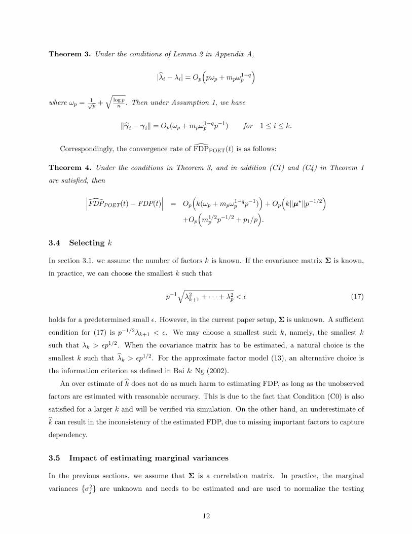
Figure 3 compares the performance of our POET-PFA estimator involving least squares estima-

tion, Efron’s method, FAMT, and FAMT-PFA. The sample size n = 50. Our POET-PFA method

estimates the true FDP(t) very well. Efron’s method captures the general trend of FDP(t) when

the true values are relatively small and deviates away from the true values in the opposite direction

when FDP(t) becomes large. FAMT-PFA performs much better than FAMT, but still could not

capture the true value when FDP(t) is large.

In Table 2, we calculate the mean and standard deviation of the direct error (the difference

between the estimated FDP and true FDP) for the four methods. Compared with three other

methods, our POET-PFA method is nearly unbiased with the smallest variance. The standard

16

deviations of direct errors for our POET-PFA method decreases when the sample size n increases.

0.0 0.4 0.8

0.0

0.4

0.8

POET-PFA

False Discovery Proportion

Est

imat

ed F

DP

_PO

ET

0.0 0.4 0.8

0.0

0.4

0.8

Efron

False Discovery Proportion

Est

imat

ed F

DP

0.0 0.4 0.8

0.0

0.4

0.8

FAMT

False Discovery Proportion

Est

imat

ed F

DP

0.0 0.4 0.8

0.0

0.4

0.8

FAMT-PFA

False Discovery Proportion

Est

imat

ed F

DP

0.0 0.4 0.8

0.0

0.4

0.8

POET-PFA

False Discovery Proportion

Est

imat

ed F

DP

_PO

ET

0.0 0.4 0.8

0.0

0.4

0.8

Efron

False Discovery Proportion

Est

imat

ed F

DP

0.0 0.4 0.8

0.0

0.4

0.8

FAMT

False Discovery Proportion

Est

imat

ed F

DP

0.0 0.4 0.8

0.0

0.4

0.8

FAMT-PFA

False Discovery Proportion

Est

imat

ed F

DP

Figure 3: Comparison of realized values of False Discovery Proportion with FDPPOET(t) involvingleast-squares estimation, Efron (2007) estimator, FAMT, and FAMT-PFA. Top panel correspondsto an approximate factor model and bottom panel corresponds to a strict factor model.

Table 2: Means and standard deviations (in parentheses) of the direct error (DE) between true

FDP(t) and the estimators FDPPOET(t) with least-squares estimation, Efron (2007) estimator,FAMT and FAMT-PFA. The results are in percent.

POET-PFA Efron FAMT FAMT-PFA

Approximaten = 50 0.19(7.54) 10.26(19.22) −10.64(15.82) −3.39(11.06)n = 100 0.75(6.58) 9.92(19.53) −10.56(15.51) −3.15(10.10)n = 200 1.01(6.21) 9.87(20.26) −11.29(15.82) −3.74(10.30)n = 500 0.89(5.15) 10.69(19.15) −11.23(15.64) −3.68(10.12)

Strictn = 50 −0.31(7.61) 10.77(21.17) −10.66(16.02) −3.83(11.41)n = 100 0.74(6.24) 9.94(21.16) −10.61(15.84) −3.56(10.43)n = 200 0.96(5.01) 8.41(21.68) −9.96(15.78) −3.49(10.55)n = 500 0.81(4.20) 10.58(20.41) −10.97(15.81) −3.94(10.26)

Robustness in overestimating the number of factors. In section 3.4, we have explained

that our POET-PFA method is robust to the overestimation of k. Figure 4 illustrates this phe-

17

nomenon, in which the direct errors for FDPPOET(t) is computed for the number of factors K

ranging from 3 to 10 while we fix k = 3 in the simulation set up. To save space, we only present the

results under approximate factor model. The figure provides the stark evidence that over estimates

of k does not hurt much as long as we can accurately estimate the common factors.

3 4 5 6 7 8 9 10

-0.4

0.0

0.4

K

Error

Figure 4: Box plots of direct errors for FDPPOET(t) involving least squares estimation when thenumber of factors ranges from K = 3, · · · , 10. The sample size n = 50. The simulation is under anapproximate factor model.

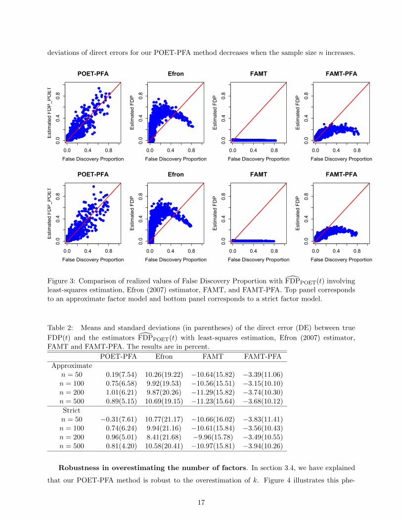
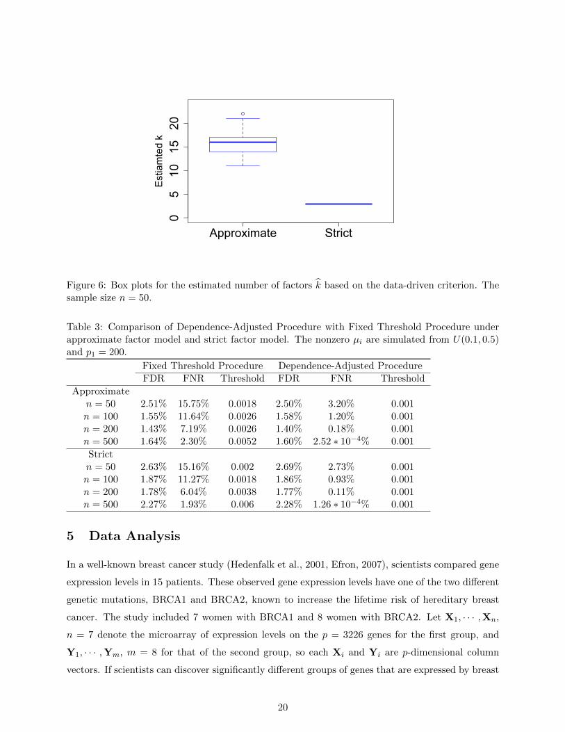
Data-driven estimate of k. In this simulation study, we will apply a data-driven method to

estimate the number of factors k. This criterion is based on expression (17) in Section 3.4. We

choose the smallest k such that λk > εp1/2 where ε = 0.1. In each simulation round, the k depends

on the generated data and can vary across simulations. Figure 5 summarizes the performance of

FDPPOET(t) based on this data-driven estimation of k. To save space, we only present the results

for the least squares estimation. Figure 6 further illustrates the distribution of the estimated k.

When n = 100, 200, 500, k = 3 for both the structure models. Here, we only present the box plot

of estimated k for n = 50. Although k varies across simulation rounds, the FDPPOET(t) performs

well as illustrated by Figure 5.

Dependence adjusted testing procedure. We compare the dependence-adjusted procedure

described in section 3.5 with the fixed threshold procedure, that is, compare the |Zi| with a universal

threshold without using the correlation information. Define the false negative rate FNR = E[T/(p−

R)] where T is the number of falsely accepted null hypotheses. With the same FDR level, a

procedure with smaller false misdiscovery rate is more powerful.

In Table 3, we fix threshold value t = 0.001 and reject the hypotheses when the dependence-

18

0.0 0.4 0.8

0.0

0.4

0.8

n=50

False Discovery Proportion

Est

imat

ed F

DP

_PO

ET

0.0 0.4 0.8

0.0

0.4

0.8

n=100

False Discovery Proportion

Est

imat

ed F

DP

_PO

ET

0.0 0.4 0.8

0.0

0.4

0.8

n=200

False Discovery Proportion

Est

imat

ed F

DP

_PO

ET

0.0 0.4 0.8

0.0

0.4

0.8

n=50

False Discovery Proportion

Est

imat

ed F

DP

_PO

ET

0.0 0.4 0.8

0.0

0.4

0.8

n=100

False Discovery Proportion

Est

imat

ed F

DP

_PO

ET

0.0 0.4 0.8

0.0

0.4

0.8

n=200

False Discovery ProportionE

stim

ated

FD

P_P

OE

T

Figure 5: Comparison of realized values of False Discovery Proportion with their estimatorsFDPPOET(t) involving least squares estimation with application of the data-driven estimation ofunknown k. The three columns from left to right correspond to n = 50, 100, 200 respectively. Thetwo rows from top to bottom correspond to approximate factor model and strict factor model.

adjusted p-values is smaller than 0.001. Then we find the corresponding threshold value for the fixed

threshold procedure such that the FDR in the two testing procedures are approximately the same.

To highlight the advantage of dependence-adjusted procedure, we reset Σu as 0.1Σ3. The FNR

for the dependence-adjusted procedure is smaller than that of the fixed threshold procedure, which

suggests that dependence-adjusted procedure is more powerful. In Fan, Han & Gu (2012), they have

shown numerically that if the covariance is known, the advantage of dependence-adjusted procedure

is even more substantial. Note that in Table 3, p1 = 200 compared with p = 1000, implying that

the better performance of the dependence-adjusted procedure is not limited to sparse situation.

This is expected since subtracting common factors out make the problem have a higher signal to

noise ratio.

19

Approximate Strict

05

1015

20E

stia

mte

d k

Figure 6: Box plots for the estimated number of factors k based on the data-driven criterion. Thesample size n = 50.

Table 3: Comparison of Dependence-Adjusted Procedure with Fixed Threshold Procedure underapproximate factor model and strict factor model. The nonzero µi are simulated from U(0.1, 0.5)and p1 = 200.

Fixed Threshold Procedure Dependence-Adjusted ProcedureFDR FNR Threshold FDR FNR Threshold

Approximaten = 50 2.51% 15.75% 0.0018 2.50% 3.20% 0.001n = 100 1.55% 11.64% 0.0026 1.58% 1.20% 0.001n = 200 1.43% 7.19% 0.0026 1.40% 0.18% 0.001n = 500 1.64% 2.30% 0.0052 1.60% 2.52 ∗ 10−4% 0.001

Strictn = 50 2.63% 15.16% 0.002 2.69% 2.73% 0.001n = 100 1.87% 11.27% 0.0018 1.86% 0.93% 0.001n = 200 1.78% 6.04% 0.0038 1.77% 0.11% 0.001n = 500 2.27% 1.93% 0.006 2.28% 1.26 ∗ 10−4% 0.001

5 Data Analysis

In a well-known breast cancer study (Hedenfalk et al., 2001, Efron, 2007), scientists compared gene

expression levels in 15 patients. These observed gene expression levels have one of the two different

genetic mutations, BRCA1 and BRCA2, known to increase the lifetime risk of hereditary breast

cancer. The study included 7 women with BRCA1 and 8 women with BRCA2. Let X1, · · · ,Xn,

n = 7 denote the microarray of expression levels on the p = 3226 genes for the first group, and

Y1, · · · ,Ym, m = 8 for that of the second group, so each Xi and Yi are p-dimensional column

vectors. If scientists can discover significantly different groups of genes that are expressed by breast

20

cancers with BRCA1 mutations and those with BRCA2 mutations, they will be able to identify

cases of hereditary breast cancer on the basis of gene-expression profiles.

Assume the gene expressions of the two groups on each microarray are from two multivari-

ate normal distributions with (potentially) different mean vector but the same covariance matrix,

namely, Xi ∼ Np(µX ,Σ) for i = 1, · · · , n and Yi ∼ Np(µ

Y ,Σ) for i = 1, · · · ,m. Then identifying

differentially expressed genes is essentially a multiple hypothesis test on

H0j : µXj = µYj vs H1j : µXj 6= µYj j = 1, · · · , p.

Consider the test statistics Z =√nm/(n+m)(X −Y) where X and Y are the sample averages.

Then we have Z ∼ Np(µ,Σ) with µ =√nm/(n+m)(µX − µY ), and the above two-sample

comparison problem is equivalent to simultaneously testing

H0j : µj = 0 vs H1j : µj 6= 0 j = 1, · · · , p

based on Z and the unknown covariance matrix Σ. It is also reasonable to assume that a large

proportion of the genes are not differentially expressed, so that µ is sparse.

0 200 400 600 800 1000

0.00

0.10

0.20

# of total rejections

Est

imat

ed F

DP

k = 2k = 3k=4k=5

0 200 400 600 800 1000

050

100

150

200

250

# of total rejections

Est

imat

ed #

of f

alse

reje

ctio

ns

k = 2k = 3k=4k=5

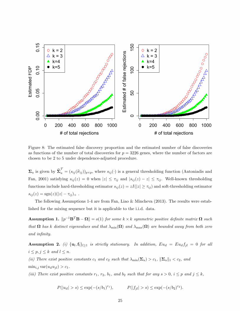
Figure 7: The estimated false discovery proportion and the estimated number of false discoveriesas functions of the number of total discoveries for p = 3226 genes, where the number of factors arechosen to be 2 to 5.

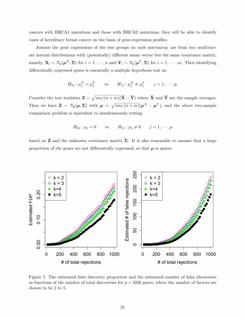
21

Approximate factor model structure has gained increasing popularity among biologists in the

past decade, since it has been widely acknowledged that gene activities are usually driven by a

small number of latent variables. See, for example, Leek & Storey (2008), Friguet, Kloareg &

Causeur (2009) and Desai & Storey (2012) for more details. We therefore apply the POET-PFA

procedure (see Section 3.3) to the dataset to obtain a consistent FDP estimator FDPPOET(t) for

given threshold value t and fixed number of factors k. The results of our analysis are depicted in

Figure 7. As can be seen, both FDPPOET(t) and V (t) increase with larger R(t), and FDPPOET(t)

is fairly close to zero when R(t) is below 200, suggesting that the rejected hypotheses in this range

have high accuracy to be the true discoveries. Secondly, even when as many as 1000 hypotheses,

corresponding to almost 1/3 of the total number, have been rejected, the estimated FDPs are as

low as 25%. Finally it is worth noting that although our procedure seems robust under different

choices of number of factors, the estimated FDP tends to be relatively small with larger number of

factors.

We also apply the dependence-adjusted procedure to the data. The relationship of estimated

FDP and number of total rejections are summarized in Figure 8. Compared with Figure 7, the

estimated FDP tends to be smaller with the same amount of total rejections. The same phenomenon

also happens to the estimated number of false rejections. This is consistent with the fact that the

factor-adjusted test is more powerful.

We conclude our analysis by presenting the list of 40 most differentially expressed genes in Tables

4 and 5 with POET-PFA method and the dependence-adjusted procedure respectively. Table 5

provides an alternative ranking of statistically significantly expressed genes for biologists, which

have a lower false discovery proportion than the conventional method presented in Table 4.

6 Appendix

6.1 Appendix A

Adaptive Thresholding Method. This method is a modification of the adaptive threshold-

ing method in Cai & Liu (2011) and has been introduced in Fan, Liao & Mincheva (2013). In

the approximate factor model, define X = (X1 − X, · · · ,Xn − X), FT

= (f1, · · · , fn), where the

columns of F/√n are the eigenvectors corresponding to the k largest eigenvalues of X

TX. Let

B = (λ1/21 γ1, · · · , λ

1/2k γk). Compute ul = (Xl −X)− Bfl,

σij =1

n

n∑l=1

uilujl, and θ 2ij =

1

n

n∑l=1

(uilujl − σij)2.

For the threshold τi,j = Cθijωp with a large enough C, the adaptive thresholding estimation for

22

Table 4: 40 most differentially expressed genes that can discriminate breast cancers with BRCA1mutations from those with BRCA2 mutations. The estimated FDP is approximately 0.0139% underapproximate factor model with 3 factors, providing strong evidence for our selection.

Clone ID UniGene Title26184 phosphofructokinase, platelet810057 cold shock domain protein A46182 CTP synthase813280 adenylosuccinate lyase950682 phosphofructokinase, platelet840702 SELENOPHOSPHATE SYNTHETASE ; Human selenium donor protein784830 D123 gene product841617 Human mRNA for ornithine decarboxylase antizyme, ORF 1 and ORF 2563444 forkhead box F1711680 zinc finger protein, subfamily 1A, 1 (Ikaros)949932 nuclease sensitive element binding protein 175009 EphB4566887 chromobox homolog 3 (Drosophila HP1 gamma)841641 cyclin D1 (PRAD1: parathyroid adenomatosis 1)809981 glutathione peroxidase 4 (phospholipid hydroperoxidase)236055 DKFZP564M2423 protein293977 ESTs, Weakly similar to putative [C.elegans]295831 ESTs, Highly similar to CGI-26 protein [H.sapiens]236129 Homo sapiens mRNA; cDNA DKFZp434B1935247818 ESTs814270 polymyositis/scleroderma autoantigen 1 (75kD)130895 ESTs548957 general transcription factor II, i, pseudogene 1212198 tumor protein p53-binding protein, 2293104 phytanoyl-CoA hydroxylase (Refsum disease)82991 phosphodiesterase I/nucleotide pyrophosphatase 132790 mutS (E. coli) homolog 2 (colon cancer, nonpolyposis type 1)291057 cyclin-dependent kinase inhibitor 2C (p18, inhibits CDK4)344109 proliferating cell nuclear antigen366647 butyrate response factor 1 (EGF-response factor 1)366824 cyclin-dependent kinase 4471918 intercellular adhesion molecule 2136769 TATA box binding protein (TBP)23014 mitogen-activated protein kinase 126184 phosphofructokinase, platelet29054 ARP1 (actin-related protein 1, yeast) homolog A (centractin alpha)36775 hydroxyacyl-Coenzyme A dehydrogenase42888 interleukin enhancer binding factor 2, 45kD45840 splicing factor, arginine/serine-rich 451209 protein phosphatase 1, catalytic subunit, beta isoform

23

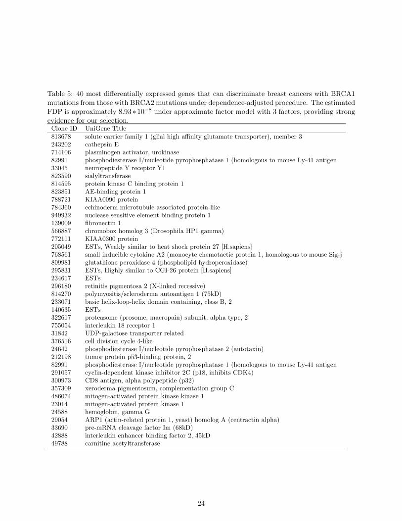
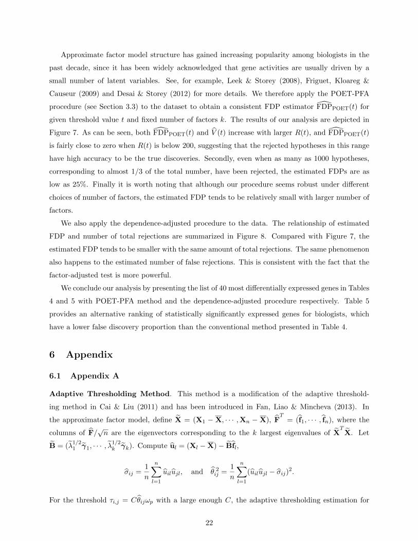
Table 5: 40 most differentially expressed genes that can discriminate breast cancers with BRCA1mutations from those with BRCA2 mutations under dependence-adjusted procedure. The estimatedFDP is approximately 8.93 ∗ 10−8 under approximate factor model with 3 factors, providing strongevidence for our selection.

Clone ID UniGene Title813678 solute carrier family 1 (glial high affinity glutamate transporter), member 3243202 cathepsin E714106 plasminogen activator, urokinase82991 phosphodiesterase I/nucleotide pyrophosphatase 1 (homologous to mouse Ly-41 antigen33045 neuropeptide Y receptor Y1823590 sialyltransferase814595 protein kinase C binding protein 1823851 AE-binding protein 1788721 KIAA0090 protein784360 echinoderm microtubule-associated protein-like949932 nuclease sensitive element binding protein 1139009 fibronectin 1566887 chromobox homolog 3 (Drosophila HP1 gamma)772111 KIAA0300 protein205049 ESTs, Weakly similar to heat shock protein 27 [H.sapiens]768561 small inducible cytokine A2 (monocyte chemotactic protein 1, homologous to mouse Sig-j809981 glutathione peroxidase 4 (phospholipid hydroperoxidase)295831 ESTs, Highly similar to CGI-26 protein [H.sapiens]234617 ESTs296180 retinitis pigmentosa 2 (X-linked recessive)814270 polymyositis/scleroderma autoantigen 1 (75kD)233071 basic helix-loop-helix domain containing, class B, 2140635 ESTs322617 proteasome (prosome, macropain) subunit, alpha type, 2755054 interleukin 18 receptor 131842 UDP-galactose transporter related376516 cell division cycle 4-like24642 phosphodiesterase I/nucleotide pyrophosphatase 2 (autotaxin)212198 tumor protein p53-binding protein, 282991 phosphodiesterase I/nucleotide pyrophosphatase 1 (homologous to mouse Ly-41 antigen291057 cyclin-dependent kinase inhibitor 2C (p18, inhibits CDK4)300973 CD8 antigen, alpha polypeptide (p32)357309 xeroderma pigmentosum, complementation group C486074 mitogen-activated protein kinase kinase 123014 mitogen-activated protein kinase 124588 hemoglobin, gamma G29054 ARP1 (actin-related protein 1, yeast) homolog A (centractin alpha)33690 pre-mRNA cleavage factor Im (68kD)42888 interleukin enhancer binding factor 2, 45kD49788 carnitine acetyltransferase

24

0 200 400 600 800 1000

0.00

0.05

0.10

0.15

# of total rejections

Est

imat

ed F

DP

k = 2k = 3k=4k=5

0 200 400 600 800 10000

50100

150

# of total rejections

Est

imat

ed #

of f

alse

reje

ctio

ns

k = 2k = 3k=4k=5

Figure 8: The estimated false discovery proportion and the estimated number of false discoveriesas functions of the number of total discoveries for p = 3226 genes, where the number of factors arechosen to be 2 to 5 under dependence-adjusted procedure.

Σu is given by ΣTu = (sij(σij))p×p, where sij(·) is a general thresholding function (Antoniadis and

Fan, 2001) satisfying sij(z) = 0 when |z| ≤ τij and |sij(z) − z| ≤ τij . Well-known thresholding

functions include hard-thresholding estimator sij(z) = zI(|z| ≥ τij) and soft-thresholding estimator

sij(z) = sgn(z)(|z| − τij)+ .

The following Assumptions 1-4 are from Fan, Liao & Mincheva (2013). The results were estab-

lished for the mixing sequence but it is applicable to the i.i.d. data.

Assumption 1. ‖p−1BTB−Ω‖ = o(1) for some k× k symmetric positive definite matrix Ω such

that Ω has k distinct eigenvalues and that λmin(Ω) and λmax(Ω) are bounded away from both zero

and infinity.

Assumption 2. (i) ul, fll≥1 is strictly stationary. In addition, Euil = Euilfjl = 0 for all

i ≤ p, j ≤ k and l ≤ n.

(ii) There exist positive constants c1 and c2 such that λmin(Σu) > c1, ‖Σu‖1 < c2, and

mini,j var(uilujl) > c1.

(iii) There exist positive constants r1, r2, b1, and b2 such that for any s > 0, i ≤ p and j ≤ k,

P (|uil| > s) ≤ exp(−(s/b1)r1), P (|fjl| > s) ≤ exp(−(s/b2)

r2).

25

We introduce the strong mixing conditions to conduct asymptotic analysis of the least square

estimates. Let F0−∞ and F∞n denote the σ-algebras generated by (fs,us) : −∞ ≤ s ≤ 0 and

(fs,us) : n ≤ s ≤ ∞ respectively. In addition, define the mixing coefficient

α(n) = supA∈F0

−∞,B∈F∞n|P (A)P (B)− P (AB)|.

Note that for the independence sequence, α(n) = 0.

Assumption 3. There exists r3 > 0 such that 3r−11 + 1.5r−12 + r−13 > 1, and C > 0 satisfying

α(n) ≤ exp(−Cnr3) for all n.

Assumption 4. Regularity conditions: There exists M > 0 such that for all i ≤ p, t ≤ n and

s ≤ n,

(i) ‖bj‖max < M ,

(ii) E[p−1/2(u′sut −Eu′sut)]4 < M ,

(iii) E‖p−1/2∑p

i=1 biuit‖4 < M .

Lemma 2. (Fan, Liao & Mincheva, 2013, Theorem 1)

Let γ−1 = 3γ−11 + 1.5γ−12 + γ−13 + 1. Suppose log p = o(nγ/6) and n = o(p2). Under Assumptions

1-4 in Appendix A,

‖ΣTu −Σu‖ = Op(ω

1−qp mp).

Define V = diag(λ1, · · · , λk). FT

= (f1, · · · , fn), and H = 1nV−1F

TFBTB, where F has been

defined in Adaptive Thresholding Method.

Lemma 3. (Fan, Liao & Mincheva, 2013, Lemma C.10 and C.12) With the same conditions

in Lemma 2,

‖H‖ = Op(1)

‖HTH− Ik‖F = Op(1√n

+1√p

)

‖B−BHT ‖2F = Op(ω2pp).

6.2 Appendix B

Proof of Proposition 1: In Proposition 2 of Fan, Han & Gu (2012), we can show that

Var(p−10 V (t)|W1, · · · ,Wk) = Op(p−δ).

26

This implies that

| 1

p0V (t)− 1

p0

∑i∈true nulls

P (Pi ≤ t|W1, · · · ,Wk)| = Op(p−δ/2).

By (C1), the desired conclusion follows.

Proof of Theorem 1: First of all, note that by (11), we have

BW = B(BTB)−1B

TZ = (

k∑i=1

γiγTi )Z. (18)

Similarly, let B = (√λ1γ1, · · · ,

√λkγk) and W = (BTB)−1BTZ. Then,

BW = (k∑i=1

γiγTi )Z. (19)

Denote by FDP1(t) the estimator in equation (7) with using the infeasible estimator W. Then,

FDPU (t)− FDPA(t) = [FDPU (t)− FDP1(t)] + [FDP1(t)− FDPA(t)].

We will bound these two terms separately.

Let us deal with the first term. Define

∆1 =

p∑i=1

[Φ(ai(zt/2 + b

T

i W))− Φ(ai(zt/2 + bTi W))]

and

∆2 =

p∑i=1

[Φ(ai(zt/2 − b

T

i W))− Φ(ai(zt/2 − bTi W))].

Then, we have

FDPU (t)− FDP1(t) = (∆1 + ∆2)/R(t). (20)

We now deal with the term ∆1 =∑p

i=1 ∆1i, in which

∆1i = Φ(ai(zt/2 + bT

i W))− Φ(ai(zt/2 + bTi W))

+Φ(ai(zt/2 + bTi W))− Φ(ai(zt/2 + bTi W))

≡ ∆11i + ∆12i.

∆2 can be dealt with analogously and hence omitted. For ∆12i, by the mean-value theorem, there

27

exists a∗i ∈ (ai, ai) such that

∆12i = φ(a∗i (zt/2 + bTi W))(ai − ai)(zt/2 + bTi W).

Since ai > 1 and ai > 1, we have a∗i > 1 and hence φ(a∗i (zt/2 + bTi W))|zt/2 + bTi W| is bounded. In

other words,

|p∑i=1

∆12i| ≤ Cp∑i=1

|ai − ai|,

for a generic constant C. Using the definition of ai and ai, we have

|ai − ai| = |(1− ‖bi‖2)−1/2 − (1− ‖bi‖2)−1/2|.

Using the mean-value theorem again, together with the assumption (C4), we have

|(1− ‖bi‖2)−1/2 − (1− ‖bi‖2)−1/2| ≤ C(‖bi‖2 − ‖bi‖2).

Let γh = (γ1h, · · · , γph)T and γh = (γ1h, · · · , γph)T . Then

p∑i=1

∣∣∣‖bi‖2 − ‖bi‖2∣∣∣ =

p∑i=1

∣∣∣ k∑h=1

(λh − λh)γ2ih +

k∑h=1

λh(γ2ih − γ2ih)∣∣∣

≤k∑

h=1

|λh − λh|+k∑

h=1

λh

p∑i=1

|γ2ih − γ2ih|,

where we used∑p

i=1 γ2ih = 1. The second term of the last expression can be bounded as

p∑i=1

|γ2ih − γ2ih| ≤( p∑i=1

|γih − γih|2p∑i=1

|γih + γih|2)1/2

≤ ‖γh − γh‖

2

p∑i=1

(γ2ih + γ2ih)1/2

= 2‖γh − γh‖.

Combining all the results that we have obtained, we have concluded that

|p∑i=1

∆12i| ≤ C( k∑h=1

|λh − λh|+ λh‖γh − γh‖). (21)

Therefore, by using∑k

h=1 λh < p and Assumptions (C2) and (C3), we conclude that |∑p

i=1412i| =

Op(p1−min(δ,κ)).

We now deal with the term ∆11i. By the mean-value theorem, there exists ξi between bT

i W

28

and bTi W such that

∆11i = φ(ai(zt/2 + ξi))ai(bT

i W − bTi W).

By (C4), ai is bounded and so is φ(ai(zt/2 + ξi))ai. Let 1 be a p-dimensional vector with each

element being 1. Then, by (18) and (19), we have

p∑i=1

|bT

i W − bTi W| ≤ 1T |BW −BW|

= 1T∣∣∣ k∑h=1

[γhγTh − γhγ

Th ]Z

∣∣∣,≤ √

p∥∥∥ k∑h=1

[γhγTh − γhγ

Th ]∥∥∥‖Z‖ (22)

where |a| = (|a1|, · · · , |ap|)T for any vector a and the last inequality is obtained by the Cauchy-

Schwartz inequality.

We now deal with the two factors in (22). The first factor is easily bounded by

k∑h=1

‖γh(γh − γh)T + (γh − γh)γTh ‖ ≤ 2k∑

h=1

‖γh − γh‖,

which is controlled by Op(kp−κ) by condition (C2). Let εipi=1 be a sequence of i.i.d. N(0, 1)

random variables. Then, stochastically, we have

‖Z‖2 ≤ 2‖µ?‖2 + 2

p∑i=1

λiε2i = Op(‖µ?‖2 + p),

because

E(

p∑i=1

λiε2i )

2 ≤ 3(

p∑i=1

λi)2 = 3p2.

Substituting these two terms into (22), we have

p∑i=1

|bT

i W − bTi W| = Op

(kp1/2−κ(‖µ∗‖+ p1/2)

).

Therefore, we can conclude that

|p∑i=1

∆11i| = Op

(kp1/2−κ(‖µ∗‖+ p1/2)

). (23)

29

Combination of the results in (21) and (23) leads to

∆1 = Op(p1−min(κ,δ)) +Op(kp

1−κ) +Op(k‖µ?‖p1/2−κ).

By (C1), R(t)/p > H, then we have |FDPU (t)− FDP1(t)| as the convergence rate in Theorem 1.

In FDP1(t), the least-squares estimator is

W = (BTB)−1BTµ? + W + (BTB)−1BTK = W + (BTB)−1BTµ? (24)

in which we utilize the orthogonality between B and var(K). With a similar argument as above,

we can show that ∣∣FDP1(t)− FDPA(t)∣∣ = O

(1T |B(W−W)|/R(t)

),

and we have

(1, · · · , 1)|B(W−W)| = 1T |(k∑

h=1

γhγTh )µ?| ≤ kp1/2‖µ?‖2.

In the second step we used the Cauchy-Schwartz inequality and the fact that ‖γi‖ = 1. Then by

(C1), the conclusion is correct. The proof is now complete.

Proof of Theorem 2: By the triangular inequality,

|λi − λi+1| ≥∣∣|λi − λi+1| − |λi+1 − λi+1|

∣∣By Weyl’s Theorem in Lemma 1, |λi+1 − λi+1| ≤ ‖Σ−Σ‖. Therefore,

|λi − λi+1| ≥ dp − ‖Σ−Σ‖ ≥ dp/2

with probability tending to one. Similarly, with probability tending to one, we have |λi−1 − λi| ≥

dp/2. By the sin θ Theorem in Lemma 1, ‖γi − γi‖ = Op(p−τ ). Hence, Condition (C2) holds with

κ = τ . Using Weyl’s Theorem again, we have

k∑i=1

|λi+1 − λi+1| ≤ k‖Σ−Σ‖ = Op(kdpp−τ ).

Hence, (C3) holds with p−δ = kp−τdp/p. The result now follows from Theorem 1.

Proof of Theorem 3. Let B = (λ1/21 γ1, · · · , λ

1/2k γk). Note that

‖ΣPOET −Σ‖ ≤ ‖BBT−BBT ‖+ ‖Σ

Tu −Σu‖. (25)

30

The bound for the second term is given by Lemma 2. We now consider the first term in (25). By

the triangular inequality, it follows that

‖BBT−BBT ‖ ≤ ‖B(HTH− Ik)B

T ‖+ ‖BHT (B−BHT )T ‖+ ‖(B−BHT )HBT ‖

+‖(B−BHT )(B−BHT )T ‖

≤ ‖HTH− Ik‖‖B‖2 + 2‖B‖‖H‖‖B−BHT ‖+ ‖(B−BHT )‖2. (26)

Recall bjkj=1 are columns of B. Without loss of generality, assume ‖bj‖ are in non-

increasing order. Since BTB is diagonal, BBT has nonvanishing eigenvalues ‖bj‖2Kj=1 and

‖B‖ = ‖b1‖. Furthermore, by Weyl’s Theorem in Lemma 1,

∣∣∣λi − ‖bi‖2∣∣∣ ≤ ‖Σ−BBT ‖ = ‖Σu‖.

Since the operator norm is bounded by the L1-norm, we have

‖Σu‖ ≤ maxi≤p

p∑j=1

|σu,ij |q|σu,iiσu,jj |(1−q)/2 ≤ mp. (27)

Hence,

‖bi‖2 ≤ λ1 +mp = O(p).

We are now bounding each term in (26). Since the operator norm is bounded by the Frobenius

norm, by Lemma 3, the first term in (26) is bounded by Op(pωp), the second term in (26) is of

order Op(ωp√p) and the third term in (26) is Op(ω

2p). Combination of these results leads to

‖BBT−BB‖ = Op(pωp).

Substituting this into (25), by Lemma 2, we have

‖ΣPOET −Σ‖ = Op(pωp +mpω1−qp ).

By Weyl’s Theorem in Lemma 1, the conclusion for |λi − λi| follows.

Assumption 1 and Weyl’s theorem imply that λi = cip + o(p) for i = 1, · · · , k and ci’s are

distinct. By the triangular inequality,

|λi − λi+1| ≥∣∣|λi − λi+1| − |λi+1 − λi+1|

∣∣.By part (i), |λi+1 − λi+1| = op(p). Therefore, for sufficiently large n, |λi − λi+1| ≥ cip for some

31

constant ci > 0. By sin θ Theorem,

‖γi − γi‖ = Op(ωp +mpω1−qp p−1).

This completes the proof.

Proof of Theorem 4: With direct application of Theorems 1 & 3, we have

∣∣∣FDPPOET(t)− FDPA(t)∣∣∣ = Op

(k(ωp +mpω

1−qp p−1)

)+Op

(k‖µ?‖p−1/2

).

Similar to (27),

p−2∑i

∑j

|σu,ij | ≤ p−1 maxi

∑j

|σu,ij |q = mpp−1.

An examination of the proof of Theorem 1 in Fan, Han & Gu (2012) shows that if we use

p−2∑

i

∑j |ai,j | = O(p−δ) to replace (C0) where ai,j is the (i, j)th element of covariance matrix of

K in (5), then Proposition 1 also holds. Therefore,

∣∣∣FDP(t)− FDPoracle(t)∣∣∣ = Op(m

1/2p p−1/2).

The conclusion of Theorem 4 follows from |FDPoracle(t)− FDPA(t)| ≤ 2p1/R(t) = Op(p1/p).

Proof of Theorem 5:

Following the same argument in the proof of Proposition 2 of Fan, Han & Gu (2012) and the

proof of Proposition 1 in the current paper, we can show that under (C0) and (C1),

|FDPadj(t)− FDP(t)| = Op(p−δ/2 + p1/p).

The slight difference is that we change

c1,i = ai(−zt/2 − ηi), and c2,i = ai(zt/2 − ηi)

in the proof of Proposition 2 in Fan, Han & Gu (2012) to

c1,i = −zt/2 − µiai, and c2,i = zt/2 − µiai

for the current proof.

32

Change ∆1 and ∆2 in the proof of Theorem 1 to

∆1 =

p∑i=1

[Φ(zt/2/ai + bT

i W)− Φ(zt/2/ai + bTi W)]

∆2 =

p∑i=1

[Φ(zt/2/ai − bT

i W)− Φ(zt/2/ai − bTi W)].

To show the convergence rate of |FDPadj(t)−FDPadj(t)|, we deal with the term ∆1 and ∆2. Since

the term ∆2 can be dealt with analogously, we consider only the term ∆1. It can be written as∑pi=1(∆11i + ∆12i), in which

∆11i = Φ(zt/2/ai + bT

i W)− Φ(zt/2/ai + bTi W)

∆12i = Φ(zt/2/ai + bTi W)− Φ(zt/2/ai + bTi W)

For ∆12i, by the mean-value theorem, there exists a∗i ∈ (ai, ai) such that

∆12i = φ(zt/2/a∗i + bTi W)zt/2(ai − ai)/(aiai).

Using ai ≥ 1 and ai ≥ 1, by Assumption (C4), we have

|p∑i=1

∆12i| ≤ Cp∑i=1

|ai − ai|

for a generic constant C. For ∆11i, by the mean-value theorem, there exists ξi such that

∆11i = φ(zt/2/ai + ξi)(bT

i W− bTi W).

The rest of the proof now follows from the same argument in the proof of Theorem 1. This completes

the proof.

Acknowledgements

This research was partly supported by NIH Grants R01-GM072611 and R01GM100474-01 and NSF

Grant DMS-1206464. We would like to thank Dr. Weijie Gu for various assistance on this project.

References

Antoniadis, A. & Fan, J. (2001). Regularized wavelet approximations (with discussion). Journal of

American Statistical Association, 96, 939-967. (specially invited presentation at JSM 2001)

Bai, J. (2003). Inferential theory for factor models of large dimensions. Econometrica, 71, 135-171.

33

Bai, J. & Ng, S. (2002). Determining the number of factors in approximate factor mod-

els.Econometrica, 70, 191-221.

Benjamini, Y. & Hochberg, Y. (1995). Controlling the false discovery rate: a practical and powerful

approach to multiple testing. Journal of the Royal Statistical Society, Series B, 57, 289-300.

Benjamini, Y. & Yekutieli, D. (2001). The Control of the False Discovery Rate in Multiple Testing

Under Dependency. Annals of Statistics, 29, 1165-1188.

Bickel, P. & Levina, L. (2008). Regularized Estimation of Large Covariance Matrices. Annals of

Statistics, 36, 199-227.

Cai, T. & Liu, W. (2011). Adaptive thresholding for sparse covariance matrix estimation. Journal

of American Statistical Association, 106, 672-684.

Carvalho, C., Chang, J., Lucas, J., Nevins, J., Wang, Q. & West, M. (2008). High-dimensional

sparse factor modeling: applications in gene expression genomics. Jounral of American Statistical

Association, 103, 1438-1456.

Chamberlain, G. & Rothschild, M. (1983). Arbitrage, factor structure and mean-variance analysis

in large asset markets. Econometrica, 51, 1305-1324.

Davis, C. & Kahan, W. (1970). The rotation of eigenvectors by a perturbation III. SIAM Journal

on Numerical Analysis, 7, 1-46.

Desai, K.H. & Storey, J.D. (2012). Cross-dimensional inference of dependent high-dimensional data.

Journal of the American Statistical Association, 107, 135-151.

Efron, B. (2007). Correlation and Large-Scale Simultaneous Significance Testing. Journal of the

American Statistical Association, 102, 93-103.

Efron, B. (2010). Correlated Z-Values and the Accuracy of Large-Scale Statistical Estimates (with

discussion). Journal of the American Statistical Association, 105, 1042-1055.

El Karoui, N. (2008). Operator Norm Consistent Estimation of Large-dimensional Sparse Covari-

ance Matrices. Annals of Statistics, 36, 2717-2756.

Engle, R. & Watson, M. (1981). A one-factor multivariate time series model of metropolitan wage

rates. Journal of American Statistical Association, 76, 774-781.

Fan, J., Han, X. & Gu, W. (2012). Estimating False Discovery Proportion under Arbitrary Covari-

ance Dependence (with discussion). Journal of American Statistical Association, 107, 1019-1035.

34

Fan, J. & Li, R. (2001). Variable selection via nonconcave penalized likelihood and its oracle

properties. Journal of American Statistical Association,96, 1348-1360.

Fan, J., Liao, Y. & Mincheva, M. (2011). High-dimensional Covariance Matrix Estimation in Ap-

proximate Factor Models. Annals of Statistics, 39, 3320-3356.

Fan, J., Liao, Y. & Mincheva, M. (2013). Large Covariance Estimation by Thresholding Principal

Orthogonal Complements (with discussion). Journal of the Royal Statistical Society, Series B.,

to appear.

Fan, J., Tang, R. & Shi, X. (2012) Partial Consistency in Linear Model with Sparse Incidental

Parameters via Penalized Estimation. Technical Report.

Friguet, C., Kloareg, M. & Causeur, D. (2009). A Factor Model Approach to Multiple Testing

Under Dependence. Journal of the American Statistical Association, 104, 1406-1415.

Hedenfalk, I., Duggan, D., Chen, Y., et al. (2001). Gene-Expression Profiles in Hereditary Breast

Cancer. New England Journal of Medicine, 344, 539-548.

Higham, N. (1988). Computing a Nearest Symmetric Positive Semidefinite Matrix. Linear Algebra

and Applications, 103, 103-118.

Horn, R. & Johnson, C. (1990). Matrix Analysis. Cambridge Univesity Press.

Ma, Z. (2013). Sparse Principal Component Analysis and Iterative Thresholding. Annals of Statis-

tics, to appear.

Rothman, A., Levina, E. & Zhu, J. (2009). Generalized Thresholding of Large Covariance Matrices.

Journal of American Statistical Association, 104, 177-186.

Sarkar, S. (2002). Some Results on False Discovery Rate in Stepwise Multiple Testing Procedures.

Annals of Statistics, 30, 239-257.

Schwartzman, A. & Lin, X. (2011). The Effect of Correlation in False Discovery Rate Estimation.

Biometrika, 98, 199-214.

Storey, J.D. (2002). A Direct Approach to False Discovery Rates. Journal of the Royal Statistical

Society, Series B, 64, 479-498.

Storey, J.D., Taylor, J.E. & Siegmund, D. (2004). Strong Control, Conservative Point Estima-

tion and Simultaneous Conservative Consistency of False Discovery Rates: A Unified Approach.

Journal of the Royal Statistical Society, Series B, 66, 187-205.

35

Sun, W. & Cai, T. (2009). Large-scale multiple testing under dependency. Journal of the Royal

Statistical Society, Series B, 71, 393-424.

36