Embed Size (px)
Citation preview
Estimation of Husler-Reiss distributionsand Brown-Resnick processes
Sebastian EngelkeInstitut fur Mathematische Stochastik, Georg-August-Universitat Gottingen, Goldschmidtstr. 7,37077 Gottingen, Germany.
Alexander MalinowskiInstitut fur Mathematische Stochastik, Georg-August-Universitat Gottingen, Goldschmidtstr. 7,37077 Gottingen, Germany.
Zakhar KabluchkoInstitut fur Stochastik, Universitat Ulm, Helmholtzstr. 18, 89069 Ulm, Germany.
Martin SchlatherInstitut fur Mathematik, Universitat Mannheim, A5, 6, 68131 Mannheim, Germany.
Summary. Estimation of extreme-value parameters from observations in the max-domainof attraction (MDA) of a multivariate max-stable distribution commonly uses aggregated datasuch as block maxima. Since we expect that additional information is contained in the non-aggregated, single “large” observations, we introduce a new approach of inference based on amultivariate peaks-over-threshold method. We show that for any process in the MDA of the fre-quently used Husler-Reiss model or its spatial extension, the Brown-Resnick process, suitablydefined conditional increments asymptotically follow a multivariate Gaussian distribution. Thisleads to computationally efficient estimates of the Husler-Reiss parameter matrix. Further, theresults enable parametric inference for Brown-Resnick processes.A simulation study compares the performance of the new estimators to other commonly usedmethods. As an application, we fit a non-isotropic Brown-Resnick process to the extremes of12 year data of daily wind speed measurements.
Keywords: Extreme value theory; Max-stable process; Peaks-over-threshold; Poisson pointprocess; Spectral density
1. Introduction
Univariate extreme value theory is concerned with the limits of linearly normalized maximaof i.i.d. observations, namely the max-stable distributions (cf. de Haan and Ferreira (2006)).Statistical inference of the parameters is well-developed and usually based on one of thefollowing two approaches. Maximum likelihood estimation is applied to blockwise maximaof the original data, where a typical block size in environmental applications is one year.On the other hand, the peaks-over-threshold (POT) method fits a suitable Poisson pointprocess to all data that exceed a certain high threshold and thus follow approximately ageneralized Pareto distribution (cf. Davison and Smith (1990)). The advantage of the latterapproach is that it avoids discarding extreme values within the blocks that are below themaximum but nevertheless contain information on the parameters.When interested in the joint extreme behavior of multivariate quantities, there are different
arX
iv:1
207.
6886
v2 [
stat
.ME
] 2
5 Se
p 20
12
2 S. Engelke, A. Malinowski, Z. Kabluchko, M. Schlather
possibilities of ordering the data, though, the most common procedure is taking compo-nentwise maxima. In multivariate extreme value theory, a random process {ξ(t) : t ∈ T}with some index set T is called max-stable, if there exists a sequence (ηi)i∈N of independentcopies of a process {η(t) : t ∈ T} and functions cn(t) > 0, bn(t) ∈ R, n ∈ N, such that theconvergence
ξ(t) = limn→∞
cn(t)(
nmaxi=1
ηi(t)− bn(t)), t ∈ T, (1)
holds in the sense of finite dimensional distributions. In this case, the process η is saidto be in the max-domain of attraction (MDA) of ξ. Typically, T is a finite set or T =Rd, d ∈ N, for the multivariate or the spatial case, respectively. Both theory and inferenceare considerably more demanding than in the univariate framework due to the fact thatno finite-dimensional parametric model captures every possible dependence structure of amultivariate max-stable distribution (cf. Resnick (2008)). Similarly to the univariate case,a standard approach for parameter estimation of the max-stable process ξ from data in itsMDA is via componentwise block maxima, which ignores much of the information containedin the original data. Moreover, even if the exact max-stable process is available, maximumlikelihood (ML) estimation is problematic since typically only the bivariate densities of max-stable distributions are known in closed form. Composite likelihood (CL) approaches arecommon tools to avoid this difficulty (cf. Padoan et al. (2010), Davison and Gholamrezaee(2012)).Only recently, multivariate POT methods have attracted increased attention. In contrast tothe univariate case, the definition of exceedances over a certain threshold is ambiguous. Forinstance, Rootzen and Tajvidi (2006) define a multivariate generalized Pareto distribution(MGPD) as the limit distribution of some multivariate random vector in the MDA of amax-stable distribution, conditional on the event that at least one of the components islarge. A simulation study in Bacro and Gaetan (2012) shows, that these MGPD performwell in many situations, yet, again only bivariate densities in a CL framework are used sincemultivariate densities are unknown. Alternatively, exceedances can be defined as the eventthat the norm of the random vector is large, giving rise to the spectral measure (cf. Coles andTawn (1991)). Engelke et al. (2012) have recently proposed to condition a fixed componenton exceeding a high threshold, which enables new methods of inference for processes thatadmit a certain incremental or a mixed moving maxima representation.
With regard to practical application such as modeling extreme wind speed or precipita-tion data, max-stable models need to find a compromise between flexibility and tractability.There are several parametric families of multivariate extreme-value distributions (see Kotzand Nadarajah (2000)) and only few max-stable models in the spatial domain (cf. de Haanand Pereira (2006); Schlather (2002); Smith (1990)). For most of them, statistical inferenceis difficult and time-intensive. Furthermore, except for the max-stable process ξ in (1) itself,usually no further processes η in the MDA of attraction of ξ are known and thus, it lacks atheoretical connection between modeling the daily processes η and modeling the extremalprocess ξ.In many applications such as geostatistics it is natural to assume that the data is normallydistributed. Under this assumption, the only possible non-trivial limit for extreme obser-vations is the d-variate Husler-Reiss distribution (cf. Husler and Reiss (1989); Kabluchko(2011)). In fact, Hashorva (2006) and Hashorva et al. (2012) show that also other dis-tributions are attracted by the Husler-Reiss distribution. Hence, we can expect good fits
Estimation of Husler-Reiss distributions and Brown-Resnick processes 3
of this model if the daily data is close to normality. Recently, it has been shown thatthe class of Brown-Resnick processes (Brown and Resnick (1977); Kabluchko et al. (2009))constitutes the spatial analog of the Husler-Reiss distributions since the latter occur asfinite-dimensional marginals of the Brown-Resnick process. The research on both theoreti-cal properties (cf. Dombry et al. (2011); Oesting et al. (2012) for simulation methods) andpractical applications (e.g., Davison et al. (2012)) of these processes is actively ongoingat present. Statistical inference, however, was so far limited to the CL methods based onbivariate densities.
In this paper, we propose new estimation methods based on a POT approach for data inthe MDA of Husler-Reiss distributions and Brown-Resnick processes. Similarly to Engelkeet al. (2012), we consider extremal increments, i.e., increments of the data with respect to afixed component, conditional on the event, that this component is large. The great advan-tage of this approach is the fact that the extremal increments turn out to be multivariateGaussian distributed. This enables, for instance, ML estimation with the full multivariatedensity function as well as parameter estimation based on functionals of the Gaussian dis-tribution. Moreover, the concept of extremal increments as well as estimators derived fromspectral densities are shown to be suitable tools for fitting a Brown-Resnick process basedon a parametric family of variograms.
The remainder of the paper is organized as follows. Section 2 comprises the definitionsand some general properties of Husler-Reiss distributions and Brown-Resnick processes.In Section 3, we provide a result on weak convergence of suitably transformed and con-ditioned variables in the MDA of the Husler-Reiss distribution, which is the basis for ourestimation methods. It is used to derive the specific asymptotic distribution for extremalincrements (Section 3.1) and for conditioning in the spectral sense (Section 3.2). In bothcases, non-parametric estimation as well as parametric fitting of Brown-Resnick processesare considered. A simulation study is presented in Section 4, which compares the perfor-mance of the different estimators from the preceding section. As an application, in Section 5we analyze daily wind speed data from the Netherlands and use our new methods of infer-ence to model spatial extreme events. Proofs of the theoretical results can be found in theAppendix.
2. Husler-Reiss distributions and Brown-Resnick processes
In this section we briefly review some details on Husler-Reiss distributions and Brown-Resnick processes and define extremal coefficient functions as a dependence measure formax-stable processes.
2.1. Husler-Reiss distributionsThe multivariate Husler-Reiss distribution was introduced in Husler and Reiss (1989) asthe limit of suitably normalized Gaussian random vectors. Suppose that the correlationmatrix Σn in the n-th row of a triangular array of (k+ 1)-variate, zero-mean, unit-varianceGaussian distributions satisfies
Λ = limn→∞
log(n)(1 · 1> − Σn) ∈ D, (2)
4 S. Engelke, A. Malinowski, Z. Kabluchko, M. Schlather
where 1 = (1, . . . , 1)> ∈ Rk+1 and D ⊂ [0,∞)(k+1)×(k+1) denotes the space of symmetric,strictly conditionally negative definite matrices
D =
{(ai,j)0≤i,j≤k = A ∈ [0,∞)(k+1)×(k+1) : x>Ax < 0 for all x ∈ Rk+1 \ {0} s.t.
k∑i=0
xi = 0, ai,j = aj,i, ai,i = 0 for all 0 ≤ i, j ≤ k
}.
Then the normalized row-wise maxima converge to the (k + 1)-variate Husler-Reiss distri-bution which is completely characterized by the matrix Λ. Note that (1 · 1> − Σn) auto-matically lies in D if Σn is non-degenerate, n ∈ N. For any matrix Λ =
(λ2i,j
)0≤i,j≤k ∈ D,
define a family of positive definite matrices by
Ψl,m(Λ) = 2(λ2mi,m0
+ λ2mj ,m0
− λ2mi,mj
)1≤i,j≤l
,
where l runs over 1, . . . , k and m = (m0, . . . ,ml) with 0 ≤ m0 < · · · < ml ≤ k. Thedistribution function of the (k + 1)-dimensional Husler-Reiss distribution with standardGumbel margins is then given by
HΛ(x) = exp
k∑l=0
(−1)l+1∑
m:0≤m0<···<ml≤k
hl,m,Λ(xm1, . . . , xml
)
, x ∈ Rk+1, (3)
where
hl,m,Λ(y0, . . . , yl) =
∫ ∞y0
S{(yi − z + 2λ2
mi,m0
)i=1,...,l
|Ψl,m(Λ)}e−z dz,
for 1 ≤ l ≤ k and h0,m,Λ(y) = exp(−y) for m ∈ {0, . . . , k}. Furthermore, for q ∈ N andΨ ∈ Rq×q positive definite, S( · |Ψ) denotes the so-called survivor function of a q-dimensionalnormal random vector with mean vector 0 and covariance matrix Ψ, i.e., if Y ∼ N(0,Ψ)and x ∈ Rq, then S(x|Ψ) = P (Y1 > x1, . . . , Yq > xq). In the bivariate case, the distributionfunction (3) simplifies to
HΛ(x, y) = exp
{−e−xΦ
(λ+
y − x2λ
)− e−yΦ
(λ+
x− y2λ
)}, x, y ∈ R, (4)
where λ = λ0,1 ∈ [0,∞] parametrizes between independence and complete dependence forλ =∞ and λ = 0, respectively.Note that the class of Husler-Reiss distributions is closed in the sense that the lower-dimensional margins of HΛ are again Husler-Reiss distributed with parameter matrix con-sisting of the respective entries in Λ. Consequently, the distribution of the bivariate sub-vector of the i-th and j-th component only depends on the parameter λi,j . Thus, one canmodify this parameter (subject to the restriction Λ ∈ D) without affecting the other com-ponents. This flexibility was demanded in Cooley et al. (2010) as a desirable property ofmultivariate extreme value models that most models do not possess, unfortunately.
Remark 2.1. The k-variate Husler-Reiss distribution is usually given by its distribu-tion function HΛ. The density for k ≥ 3 is rather complicated and involves multivariateintegration. Hence, for maximum likelihood estimation based on block maxima, only thebivariate or sometimes the trivariate (cf. Genton et al. (2011)) densities are used in theframework of a composite likelihood approach.
Estimation of Husler-Reiss distributions and Brown-Resnick processes 5
2.2. Brown-Resnick processesFor T = Rd, d ≥ 1, let {Y (t) : t ∈ T} be a centered Gaussian process with stationaryincrements. Further, let γ(t) = E(Y (t) − Y (0))2 and σ2(t) = E(Y (t))2 be the variogramand the variance of Y , t ∈ Rd, respectively. Then, for a Poisson point process
∑i∈N δUi
onR with intensity e−udu and i.i.d. copies Yi ∼ Y , i ∈ N, the process
ξ(t) = maxi∈N
Ui + Yi(t)− σ2(t)/2, t ∈ Rd, (5)
is max-stable, stationary and its distribution only depends on the variogram γ. For thespecial case where Y is a Brownian motion, the process ξ was already introduced by Brownand Resnick (1977). Its generalization in (5) is called Brown-Resnick process associated tothe variogram γ (Kabluchko et al. (2009)). Since any conditionally negative definite functioncan be used as variogram, Brown-Resnick processes constitute an extremely flexible classof max-stable random fields. Moreover, the subclass associated to the family of fractalvariograms γα,s(·) = ‖ · /s‖α, α ∈ (0, 2], s ∈ (0,∞), arises as limits of pointwise maxima ofsuitably rescaled and normalized, independent, stationary and isotropic Gaussian randomfields (cf. Kabluchko et al. (2009)). Here ‖ · ‖ denotes the Euclidean norm. The modelby Smith (1990) is another frequently used special case of Brown-Resnick processes, whichcorresponds to the class of variograms γ(h) = ‖hΣ−1h‖, for h ∈ Rd and an arbitrarycovariance matrix Σ ∈ Rd×d.We remark that the finite-dimensional marginal distribution at locations t0, . . . , tk ∈ Rd ofa Brown-Resnick process is the Husler-Reiss distribution HΛ with Λ = (γ(ti− tj)/4)0≤i,j≤k.
2.3. Extremal coefficient functionSince, in general, covariances do not exist for extreme value distributed random vectors,other measures of dependence are usually considered, one of which being the extremalcoefficient θ. For a bivariate max-stable random vector (X1, X2) with identically distributedmargins, θ ∈ [1, 2] is determined by
P(X1 ≤ u,X2 ≤ u) = P(X1 ≤ u)θ,
for some (and hence all) u ∈ R. The quantity θ measures the degree of tail dependencewith limit cases θ = 1 and θ = 2 corresponding to complete dependence and completeindependence, respectively. For a stationary, max-stable process ξ on Rd, the extremalcoefficient function θ(h) is defined as the extremal coefficient of (ξ(0), ξ(h)), for h ∈ Rd(Schlather and Tawn (2003)).For the bivariate Husler-Reiss distribution (4) we have HΛ(u, u) = exp (−2Φ(λ)e−u) andthus, the extremal coefficient equals θ = 2Φ(λ). Hence, for Husler-Reiss distributions, thereis a one-to-one correspondence between the parameter λ ∈ [0,∞] and the set of extremalcoefficients. Similarly, the extremal coefficient function of the Brown-Resnick process in (5)is given by
θ(h) = 2Φ(√γ(h)/2), h ∈ Rd. (6)
Since there are model-independent estimators for the extremal coefficient function, e.g., themadogram in Cooley et al. (2006), it is a common tool for model checking.
6 S. Engelke, A. Malinowski, Z. Kabluchko, M. Schlather
3. Estimation
In this section, we propose new estimators for the parameter matrix Λ of the Husler-Reissdistribution and use them to fit Brown-Resnick processes based on a parametric family ofvariograms. We will consider both estimation based on extremal increments and estimationin the spectral domain.
Suppose that Xi = (X(0)i , . . . , X
(k)i ), i = 1, . . . , n, are independent copies of a random
vector X ∈ Rk+1 in the MDA of the Husler-Reiss distribution HΛ with some parametermatrix Λ = (λ2
i,j)0≤i,j≤k ∈ D. Recall that HΛ has standard Gumbel margins. Without lossof generality, we assume that X has standard exponential margins. Otherwise we could
consider (U0(X(0)i ), . . . , Uk(X
(k)i )), where Ui = − log(1 − Fi), and Fi is the cumulative
distribution function of the i-th marginal of X (cf. Prop. 5.15 in Resnick (2008)). In thesequel, we denote by Xn = X − log n and Xi,n = Xi − log n the rescaled data such thatthe empirical point process Πn =
∑ni=1 δXi,n
converges in distribution to a Poisson point
process Π on E = [−∞,∞)k+1 \{−∞} with intensity measure µ([−∞,x]C) = − logHΛ(x)(Prop. 3.21 in Resnick (2008)), as n → ∞. Based on this convergence of point processes,the following theorem provides the conditional distribution of those data which are extremein some sense.
Theorem 3.1. For m ∈ N and a metric space S, let g : Rk+1 → S be a measurabletransformation of the data and assume that it satisfies the invariance property g(x+a ·1) =g(x) for any a ∈ R and 1 = (1, . . . , 1) ∈ Rk+1. Further, let u(n) > 0, n ∈ N, be a sequenceof real numbers such that limn→∞ u(n)/n = 0. Then, for all Borel sets B ∈ B(S) andA ∈ B(E) bounded away from −∞,
limn→∞
P{g(Xn) ∈ B
∣∣ Xn ∈ A− log u(n)}
= Qg,A(B), (7)
for some probability measure Qg,A on S.
Remark 3.2. Note that due to the invariance property of g, the transformed data isindependent of the rescaling, i.e. g(Xi,n) = g(Xi), for all i = 1, . . . , n, n ∈ N.
In the above theorem, u(n) only has to satisfy u(n)/n → 0, as n tends to ∞. How-ever, for practical applications it is advisable to choose u(n) in such a manner that alsolimn→∞ u(n) = ∞, since this ensures that the cardinality of the index set of extremal ob-servations
IA ={i ∈ {1, . . . , n} : Xi,n ∈ A− log u(n)
}, (8)
tends to ∞ as n→∞, almost surely.
Theorem 3.1 implies that for all extreme events, the transformed data {g(Xi) : i ∈ IA}approximately follow the distribution Qg,A. Clearly, Qg,A depends on the choices for g andA and in the subsequent sections we encounter different possibilities for which the limit (7)can be computed explicitly. Furthermore, if g and A are chosen suitably, the distributionQg,A will still contain all information on the parameter matrix Λ. Our estimators willtherefore be based on the set of transformed data {g(Xi) : i ∈ IA} and the knowledge oftheir asymptotic distribution Qg,A. For instance, a maximum likelihood approach can beapplied using the fact that Πn converges to Π. If, for a particular realization of the Xi,
Estimation of Husler-Reiss distributions and Brown-Resnick processes 7
IA = {i1, . . . , iN} for some N ≤ n, i1, . . . , iN ∈ {1, . . . , n}, and g(Xi) = si, i = 1, . . . , n, acanonical approach is to maximize the likelihood
Lg,A(Λ; s1, . . . , sn) = P{|IA| = N, g(Xij ) ∈ dsij , j = 1, . . . , N
}= P (|IA| = N)
N∏j=1
P{g(X) ∈ dsij | Xn ∈ A− log u(n)
}.
With the Poisson approximation∑ni=1 1{Xi,n ∈ A− log u(n)} ≈ Pois{µ(A− log u(n))} and
the convergence (7) we obtain
Lg,A(Λ; s1, . . . , sn) ≈ exp{−µ(A− log u(n))}µ(A− log u(n))N
N !
N∏j=1
Qg,A(dsij ). (9)
If the ML approach is unfeasible, estimation of Λ can also be based on other suitably chosenfunctionals of the conditional distribution of g(X), for instance on the variance of g(X).
3.1. Inference based on extremal incrementsIn this subsection, we apply Theorem 3.1 with g mapping the data to its increments w.r.t.a fixed index, i.e., g : Rk+1 → Rk, x 7→ ∆x = (x(1) − x(0), . . . , x(k) − x(0)). In particular,g satisfies the invariance property g(x + a · 1) = g(x) for any a ∈ R. Consequently, ourestimators are based on the incremental distribution of those data which are extreme in thesense specified by the set A. The following theorem provides the limiting distribution Qg,Afor two particular choices of A, namely A1 = (0,∞)× Rk and A2 = [−∞,0]C .
Theorem 3.3. Let X be in the MDA of HΛ with some Λ ∈ D, and suppose that thesequence u(n) is chosen as in Theorem 3.1. Then, we have the following convergences indistribution.
(a) For k ∈ N,(X(1) −X(0), . . . , X(k) −X(0)
∣∣X(0)n > − log u(n)
)d→ N (M,Σ), n→∞,
where N (M,Σ) denotes the multivariate normal distribution with mean vector M =− diag(Ψk,(0,...,k)(Λ))/2 and covariance matrix Σ = Ψk,(0,...,k)(Λ).
(b) For the bivariate case, i.e., k = 1,(X(1) −X(0)
∣∣X(0)n > − log u(n) or X(1)
n > − log u(n))
d→ Z, n→∞,
where Z is a real-valued random variable with density given by
gλ(t) =1
4λΦ(λ)φ
(λ− |t|
2λ
), t ∈ R, λ = λ0,1.
Here, Φ and φ denote the standard normal distribution function and density, respec-tively.
8 S. Engelke, A. Malinowski, Z. Kabluchko, M. Schlather
Remark 3.4. The positive definite matrix Σ = Ψk,(0,...,k)(Λ) contains all informationon Λ. In fact, the transformation
Λ(Σ) =1
4
0 diag(Σ)>
diag(Σ) 1diag(Σ)> + diag(Σ)1> − 2Σ
recovers the matrix Λ = (λ2
i,j)0≤i,j≤k.
Based on the convergence results in Theorem 3.3 we propose various estimation pro-cedures for both multivariate Husler-Reiss distributions (non-parametric case) and Brown-Resnick processes with a parametrized family of variograms (parametric case).
3.1.1. Non-parametric multivariate caseFor the likelihood based approach in (9) we first consider the extremal set A1 = (0,∞)×Rkand put N1 = |IA1
|. By part one of Theorem 3.3 we have
− logL(Λ; s1, . . . , sn) ≈ − log
exp(−u(n))u(n)N1
N1!
N1∏j=1
φM(Λ),Σ(Λ)
(sij)
∝ N1
2log det Σ(Λ) +
1
2
N1∑j=1
{(sij −M(Λ))>Σ(Λ)−1(sij −M(Λ))
},
(10)
where si is the realization of ∆Xi, i = 1, . . . , n and φM(Λ),Σ(Λ) is the density of the nor-mal distribution with mean vector M(Λ) = −diag(Ψk,(0,...,k)(Λ))/2 and covariance matrixΣ(Λ) = Ψk,(0,...,k)(Λ). The corresponding maximum likelihood estimator is given by
ΛMLE = arg minΛ∈D
N1
2log det Σ(Λ) +
1
2
N1∑j=1
{(sij −M(Λ))>Σ(Λ)−1(sij −M(Λ))
} . (11)
Notice that for this particular choice of A, the asymptotic value of P(|IA1 | = N1) does notdepend on the parameter matrix Λ. Hence, this ML ansatz coincides with simply maximiz-ing the likelihood of the increments without considering the number of points exceeding thethreshold. In the bivariate case, i.e., k = 1 and A1 = (0,∞)× R, (10) simplifies to
− logL(λ; s1, . . . , sn) ∝ N1λ2
2+N1 log λ+
1
8λ2
N1∑j=1
s2ij , (12)
and the minimizer of (12) can be given in explicit form:
λ2MLE =
1
2
−1 +
√√√√1 +1
N1
N1∑j=1
(∆Xij )2
. (13)
Estimation of Husler-Reiss distributions and Brown-Resnick processes 9
Staying in the bivariate case, for the choice A2 = [−∞,0]C , we put N2 = |IA2 | and bypart two of Theorem 3.3,
− logL(λ; s1, . . . , sn) ≈ − log
exp(−2Φ(λ)u(n))(2Φ(λ)u(n))N2
N2!
N2∏j=1
gλ(sij )
∝ 2Φ(λ)u(n) +
N2λ2
2+
1
8λ2
N2∑j=1
s2ij .
Numerical optimization can be applied to obtain the estimator
λ2MLE2 = arg min
θ≥0
2Φ(√θ)u(n) +
N2θ
2+
1
8θ
N2∑j=1
(∆Xij )2
.
While the above likelihood-based estimators (except for (13)) require numerical opti-mization, the following approach is computationally much more efficient: A natural esti-mator for Σ = Ψk,(0,...,k)(Λ) ∈ Rk×k based on the first part of Theorem 3.3 is given by the
empirical covariance Σ of the extremal increments ∆Xi = (X(1)i − X(0)
i , . . . , X(k)i − X(0)
i )for i ∈ IA1 , i.e.
Σ =1
N1
N1∑j=1
(∆Xij − µ)(∆Xij − µ)>, µ =1
N1
N1∑j=1
∆Xij . (14)
By Remark 3.4 this also gives an estimator ΛVar = Λ(Σ) for the parameter matrix Λ, whichwe call the variance-based estimator. Apart from its simple form, another advantage of(14) is that Σ is automatically a positive definite matrix and hence, ΛVar is conditionallynegative definite and therefore a valid matrix for a (k+1)-variate Husler-Reiss distribution.Note that (14) is not the maximum likelihood estimator (MLE) for Σ since the mean of theconditional distribution of ∆Xi depends on the diagonal of Σ. The MLE of Σ is instead givenby optimizing (11) w.r.t. Σ, which, to our knowledge, does not admit a closed analyticalform.
Applying (14) with k = 1 yields the bivariate variance-based estimator
λ2Var =
1
4N1
N1∑j=1
(X(1)ij−X(0)
ij− µ)2, µ =
1
N1
N1∑j=1
(X(1)ij−X(0)
ij). (15)
Since the mean of the extremal increments is also directly related to the parameter λ,another sensible estimator might be
λ2mean = − 1
2N1
N1∑j=1
(X(1)ij−X(0)
ij). (16)
10 S. Engelke, A. Malinowski, Z. Kabluchko, M. Schlather
3.1.2. Parametric approach for Brown-Resnick processesStatistical inference for Brown-Resnick processes as in (5) is usually based on fitting aparametric variogram model {γϑ : ϑ ∈ Θ}, Θ ⊂ Rj , j ∈ N, to point estimates of the ex-tremal coefficient function (6) based on the madogram. Alternatively, composite likelihoodapproaches are used in connection with block maxima of bivariate data (Davison and Gho-lamrezaee (2012)).Since for t0, . . . , tk ∈ Rd, the vector (ξ(t0), . . . , ξ(tk)) with ξ being a Brown-Resnick processassociated to the variogram γ : Rd → [0,∞) is Husler-Reiss distributed with parametermatrix
Λ = (γ(ti − tj)/4)0≤i,j≤k,
the above estimators enable parametric estimation of Brown-Resnick processes. In fact,replacing Λ in (11) by
Λ(ϑ) = (γϑ(ti − tj)/4)0≤i,j≤k (17)
leads to the ML estimator
ϑMLE = arg minϑ∈Θ{− logL(Λ(ϑ); s1, . . . , sn)}
with L as in (10). Note that, other than in classical extreme value statistics, here the useof higher dimensional densities is feasible and promises a gain in accuracy.Estimation of ϑ can also be based on any of the bivariate estimators λ2
MLE, λ2MLE2, λ2
Var,
λ2mean, or on the multivariate estimator ΛVar by “projecting” the latter matrix or the matrix
consisting of all bivariate estimates onto the set of matrices{
(γϑ(ti− tj)/4)0≤i,j≤k:ϑ ∈ Θ}
,i.e.,
ϑPROJ = arg minϑ∈Θ
∥∥∥∥(λ2ij − γϑ(ti − tj)/4
)0≤i,j≤k
∥∥∥∥ , (18)
where ‖ · ‖ can be any matrix norm.Similar to Bacro and Gaetan (2012), the bivariate estimators can readily be used in aparametric composite likelihood framework.
3.2. Inference based on spectral densitiesAs at the beginning of Section 3, let Xi, i = 1, . . . , n, be a sequence of independent copies ofX, already standardized to exponential margins, in the MDA of the max-stable distributionHΛ. Since we work in the spectral domain in this section, we will switch to standard Frechetmargins with distribution function exp(−1/y), y ≥ 0. More precisely, we consider the vectorsY = exp(X) and Yi = exp(Xi), i = 1, . . . , n, which are in the MDA of the Husler-Reissdistribution GΛ(x) = HΛ(logx),x ≥ 0, with standard Frechet margins.The most convenient tool to characterize the dependence structure of a multivariate extremevalue distribution is via its spectral measure. To this end, let Yn = Y/n and Yi,n = Yi/ndenote the rescaled data such that the point process Pn =
∑ni=1 δYi,n
converges, as n→∞,
to a non-homogeneous Poisson point process P on [0,∞)k+1 \ {0} with intensity measureν([0,x]C) = − logGΛ(x). Transforming a vector x = (x0, . . . , xk) ∈ [0,∞)k+1 \ {0} to itspseudo-polar coordinates
r = ‖x‖, ω = r−1x, (19)
Estimation of Husler-Reiss distributions and Brown-Resnick processes 11
for any norm ‖ ·‖ on Rk+1, we can rewrite ν as a measure on (0,∞)×Sk, where Sk is the k-dimensional unit simplex Sk = {y ≥ 0 : ‖y‖ = 1}. Namely, we have ν(dx) = r−2dr×M(dω),where the measure M is called the spectral measure of GΛ and embodies the dependencestructure of the extremes. For our purposes, it is most convenient to choose the L1-norm,i.e., ‖x‖1 =
∑ki=0 |xi|. In this case, for the set Ar0 = {x ∈ [0,∞)k+1 \ {0} : ‖x‖1 > r0},
r0 > 0, we obtain
ν(Ar0) = r−10 M(Sk) = r−1
0 · (k + 1), (20)
since the measure M satisfies∫Skωi M(dω) = 1 for i = 0, . . . , k. Hence, the ν-measure of
Ar0 does not depend on the parameters of the specific model chosen for M . The distributionfunction can be written as
GΛ(x) = exp
{−∫Sk
max
(ω0
x0, . . . ,
ωkxk
)M(dω)
}, x ≥ 0.
As the space of all spectral measures is infinite dimensional, there is a need of parametricmodels which are analytically tractable and at the same time flexible enough to approximatethe dependence structure in real data sufficiently well. Parametric models are usuallygiven in terms of their spectral density h of the measure M . The book by Kotz andNadarajah (2000) gives an overview of parametric multivariate extreme value distributions,most of them, however, being only valid in the bivariate case. For the multivariate caseonly few models are known, e.g., the logistic distribution and its extensions (Joe, 1990;Tawn, 1990) and the Dirichlet distribution Coles and Tawn (1991). The recent interestin this topic resulted in new multivariate parametric models (Boldi and Davison (2007);Cooley et al. (2010)) as well as in general construction principles for multivariate spectralmeasures (Ballani and Schlather (2011)). All these approaches have in common that theypropose models for multivariate max-stable distributions in order to fit data obtained byexceedances over a certain threshold or by block maxima.Given a parametric model for the spectral density h( · ;ϑ), we have the analog result as inTheorem 3.1 for the Frechet case with A = Ar0 and g : Rk+1 → Sk,x 7→ x/‖x‖1, which nowsatisfies the multiplicative invariance property g(a · x) = g(x), for all a ∈ R. The Frechetversion of (7) for this choice of g and A reads as
limn→∞
P{Y/‖Y‖1 ∈ B | Yn ∈ Ar0/u(n)
}=
M(B)
M(Sk)=
1
k + 1
∫B
h(ω;ϑ)dω, (21)
for all B ∈ B(Sk) and u(n), n ∈ N, as in Theorem 3.1. Based on this conditional distributionof those Yi for which the sum ‖Yi‖1 is large, similarly to (9) we obtain the likelihood
LAr0
(ϑ;(r1,ω1), . . . , (rn,ωn)
)≈ exp{−ν(Ar0/u(n))}ν(Ar0/u(n))|I0|
|I0|!∏i∈I0
r−2i (k + 1)−1h(ωi;ϑ)
∝∏i∈I0
h(ωi;ϑ), (22)
where {(ri,ωi) : 1 ≤ i ≤ n} are the pseudo-polar coordinates of {Yi,n : 1 ≤ i ≤ n} as
in (19) and I0 is the set of all indices 1 ≤ i ≤ n with Yi,n ∈ Ar0/u(n). Note that the
12 S. Engelke, A. Malinowski, Z. Kabluchko, M. Schlather
proportional part in (22) only holds because the ν-measure of Ar0 is independent of themodel parameter ϑ.For the Husler-Reiss distribution it is possible to write down the spectral density h( · ; Λ)explicitly.
Proposition 3.5. For any matrix Λ =(λ2i,j
)0≤i,j≤k ∈ D the Husler-Reiss distribution
can be written as
G(x) = exp
{−∫Sk
max
(ω0
x0, . . . ,
ωkxk
)h(ω; Λ) dω
},
with spectral density
h (ω,Λ) =1
ω20 · · ·ωk(2π)k/2|det Σ|1/2
exp
(−1
2ω>Σ−1ω
), ω ∈ Sk, (23)
where Σ = Ψk,(0,...,k)(Λ) and ω = (log ωi
ω0+ 2λ2
i,0 : 1 ≤ i ≤ k)>.
3.2.1. Non-parametric, multivariate caseBased on the explicit expression for the spectral density of the Husler-Reiss distributionin (23), we define the estimator ΛSPEC of Λ as the matrix in D that maximizes the likelihoodin (22), i.e.,
ΛSPEC = arg minΛ∈D
(|I0|2
log det Ψk,(0,...,k)(Λ) +1
2
∑i∈I0
ωi>Ψk,(0,...,k)(Λ)−1ωi
). (24)
In the bivariate case, the spectral density in (23) simplifies to
h(ω;λ) =1
2λω20ω1(2π)1/2
exp
(−
(log ω1
ω0+ 2λ2)2
8λ2
)
and the corresponding estimator can be given in explicit form:
λ2SPEC =
1
2
−1 +
√1 +
1
|I0|∑i∈I0
{log(Y
(1)i
/Y
(0)i
)}2
. (25)
Note that the estimators (24) and (25) have exactly the same form as the maximum like-lihood estimators (11) and (13), respectively, for the extremal increments. However, thespecification of the set A differs and so does the choice of extreme data that is plugged in.
3.2.2. Parametric approach for Brown-Resnick processesAnalogously to Section 3.1.2, we obtain a parametric estimate of the dependence structureof a Brown-Resnick process based on a parametric family of variograms by replacing Λ onthe right-hand side of (24) by Λ(ϑ) defined in (17). This yields
ϑSPEC = arg minϑ∈Θ
{− logLAr0
(Λ(ϑ); (r1,ω1), . . . , (rn,ωn))}. (26)
Estimation of Husler-Reiss distributions and Brown-Resnick processes 13
4. Simulation study
We compare the performance of the different parametric and non-parametric estimationprocedures of Brown-Resnick processes and Husler-Reiss distributions proposed in the pre-vious section via a simulation study.
In the first instance, we consider bivariate data that is in the MDA of the Husler-Reiss distribution with known dependence parameter λ = λ0,1. For simplicity, we simulatedata from the Husler-Reiss distribution itself, which does not mean that the thresholdingprocedure via the set A becomes obsolete. All estimators rely on considering only extremalevents and hence, there is no obvious advantage over using any other data being in the MDAof Hλ. We compare the estimators λ2
MLE, λ2MLE2, λ2
Var, λ2mean and λ2
SPEC from Section 3 fordifferent sample sizes n ∈ {500, 8000, 100000}. The sequence of thresholds u(n) is chosenin such a way that the number of exceedances k(n) increases to ∞, but at the same time,the corresponding quantile q(n) = 1 − k(n)/n approaches 1, as n → ∞. In addition tothe new threshold based estimators, we include the classical estimators, which use blockmaxima, namely the madogram estimator λmado = Φ−1(θmado/2) (Cooley et al., 2006) and
the ML estimator λ2HRMLE of the bivariate Husler-Reiss distribution. To model a year of
(dependent) data, we we choose a block size of 150 which is of order of but less than 365.The pseudo-code of the exact simulation setup is the following:
(a) for λ2 ∈ {k · 0.025 : k = 1, . . . , 30}
(b) for n ∈ {500, 8000, 100000}
(c) simulate n bivariate Husler-Reiss distributionswith parameter λ
(d) for λ2 ∈{λ2
MLE, λ2MLE2, λ
2Var, λ
2mean, λ
2SPEC, λ
2mado, λ
2HRMLE
}(e) estimate λ2 through λ2
(f) obtain an estimate of the corresponding extremalcoefficient θ through θ = θ(λ) = 2Φ(λ)
(g) repeat (a)-(f) 500 times
Since the finite dimensional margins of a Brown-Resnick process are Husler-Reiss dis-tributed, we can easily implement step (a) by simulating a one-dimensional Brown-Resnickprocess with variogram γ(h) = |h| on the interval [0, 3]. Since we consider bivariate Husler-
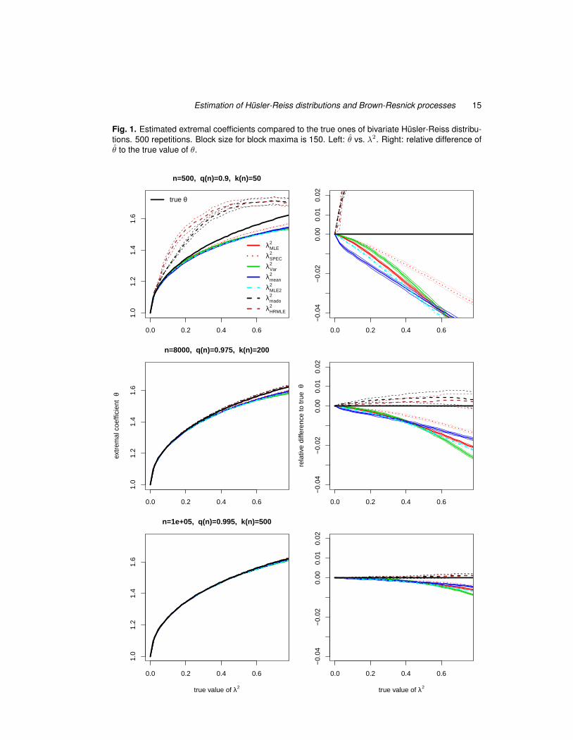
Reiss distributions for different values of λ2 lying on a fine grid, we visualize the estimates θas functions of the true λ2 (Figure 1). However, it is important to remark that estimation inthis first part of the study is exclusively based on the bivariate distributions. For each valueof λ2, we repeat simulation and estimation 500 times. Figure 1 shows the pointwise meanvalue of the extremal coefficient and the corresponding empirical 95% confidence intervals.As expected, in finite samples, all estimators based on multivariate POT methods under-estimate the true degree of extremal dependence since they are based on an asymptoticdistribution with non-zero mean while the simulated data come from a stationary process.As the sample size n and the threshold u(n) increase, all estimators approach the true
value. Among the POT-based estimators, λ2SPEC seems to be at least as good as the other
estimators, uniformly for all values of λ2 under consideration. λ2Var performs well for small
14 S. Engelke, A. Malinowski, Z. Kabluchko, M. Schlather
values of λ2 but is more biased than other estimators for large values of λ2. The goodperformance of λ2
mean for large values of λ2 might be due to the fact that it only uses firstmoments of the extremal increments and is hence less sensible to aberration of the finitesample distribution from the asymptotic distribution. Compared to the two estimatorsbased on block maxima, the POT-based estimators all perform well even for small datasets, which is a great advantage for many applications. Moreover, the variances of thePOT-estimates are generally smaller than those based on block maxima, since more datacan be used. Finally, note that the POT-based estimation does not exploit the fact, thatthe simulated data in the max-domain of attraction is in fact the max-stable distributionitself. The speed of convergence may though differ when using data from other models inthe MDA. In contrast, λ2
mado and λ2HRMLE do profit from simulating i.i.d. realizations of
the max-stable distribution itself since then, the blockwise maxima are exactly Husler-Reissdistributed and not only an approximation as in the case of real data.
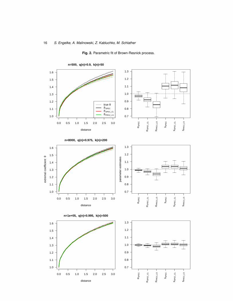
In the second part of the simulation study we examine the performance of parametricestimates of Brown-Resnick processes using the same data as above. While the true vari-ogram is γ(h) = |h|, we estimate the parameter vector (α, s) for the family of variogramsγα,s(h) = ‖h/s‖α, α ∈ (0, 2], s > 0. We compare the following three estimators: the spectral
estimator (α, s)SPEC, given by (26) and using the full multivariate density; the composite
likelihood estimator (α, s)SPEC, CL, defined as the maximizer of the product of all bivariatespectral densities, implicitly assuming independence of all tuples of locations; and the least
squares estimator (α, s)PROJ, LS, given by (18) for the Euclidean norm, where λ2MLE serves
as non-parametric input. The estimated values of α and s are compared in the right columnof Figure 2. The left panel shows the corresponding extremal coefficient functions for α ands representing the mean, the 5% sample quantile and the 95% sample quantile from the 500repetitions, respectively.
The estimator (α, s)SPEC, which incorporates the full multivariate information, performsbest both in the sense of minimal bias and minimal variance. Especially estimation of theshape parameter of the variogram gains stability when using higher-dimensional densities.The projection estimator seems to have the largest bias and the largest variance. The re-sults remain very similar if we replace λ2
MLE by one of the other non-parametric estimators.Let us finally remark that all three estimators can be modified by considering only smalldistances for inference. Then, since the approximation error of the asymptotic conditionaldistribution decays for smaller distances, this can substantially improve the accuracy in asimulation framework, but might distort the results in real data situations.
Estimation of Husler-Reiss distributions and Brown-Resnick processes 15
Fig. 1. Estimated extremal coefficients compared to the true ones of bivariate Husler-Reiss distribu-tions. 500 repetitions. Block size for block maxima is 150. Left: θ vs. λ2. Right: relative difference ofθ to the true value of θ.
0.0 0.2 0.4 0.6
1.0
1.2
1.4
1.6
n=500, q(n)=0.9, k(n)=50
true θ
λMLE2
λSPEC2
λVar2
λmean2
λMLE22
λmado2
λHRMLE2
0.0 0.2 0.4 0.6
−0.
04−
0.02
0.00
0.01
0.02
0.0 0.2 0.4 0.6
1.0
1.2
1.4
1.6
n=8000, q(n)=0.975, k(n)=200
extr
emal
coe
ffici
ent
θ
0.0 0.2 0.4 0.6
−0.
04−
0.02
0.00
0.01
0.02
rela
tive
diffe
renc
e to
true
θ
0.0 0.2 0.4 0.6
1.0
1.2
1.4
1.6
n=1e+05, q(n)=0.995, k(n)=500
true value of λ2
0.0 0.2 0.4 0.6
−0.
04−
0.02
0.00
0.01
0.02
true value of λ2
16 S. Engelke, A. Malinowski, Z. Kabluchko, M. Schlather
Fig. 2. Parametric fit of Brown-Resnick process.
0.0 0.5 1.0 1.5 2.0 2.5 3.0
1.0
1.1
1.2
1.3
1.4
1.5
1.6
n=500, q(n)=0.9, k(n)=50
distance
true θϑSPEC
ϑSPEC_CL
ϑPROJ_LS
α SP
EC
α SP
EC
_CL
α PR
OJ_
LS
s SP
EC
s SP
EC
_CL
s PR
OJ_
LS
0.7
0.8
0.9
1.0
1.1
1.2
1.3
0.0 0.5 1.0 1.5 2.0 2.5 3.0
1.0
1.1
1.2
1.3
1.4
1.5
1.6
n=8000, q(n)=0.975, k(n)=200
distance
extr
emal
coe
ffici
ent
θ
α SP
EC
α SP
EC
_CL
α PR
OJ_
LS
s SP
EC
s SP
EC
_CL
s PR
OJ_
LS
0.7
0.8
0.9
1.0
1.1
1.2
1.3
para
met
er e
stim
ates
0.0 0.5 1.0 1.5 2.0 2.5 3.0
1.0
1.1
1.2
1.3
1.4
1.5
1.6
n=1e+05, q(n)=0.995, k(n)=500
distance
α SP
EC
α SP
EC
_CL
α PR
OJ_
LS
s SP
EC
s SP
EC
_CL
s PR
OJ_
LS
0.7
0.8
0.9
1.0
1.1
1.2
1.3
Estimation of Husler-Reiss distributions and Brown-Resnick processes 17
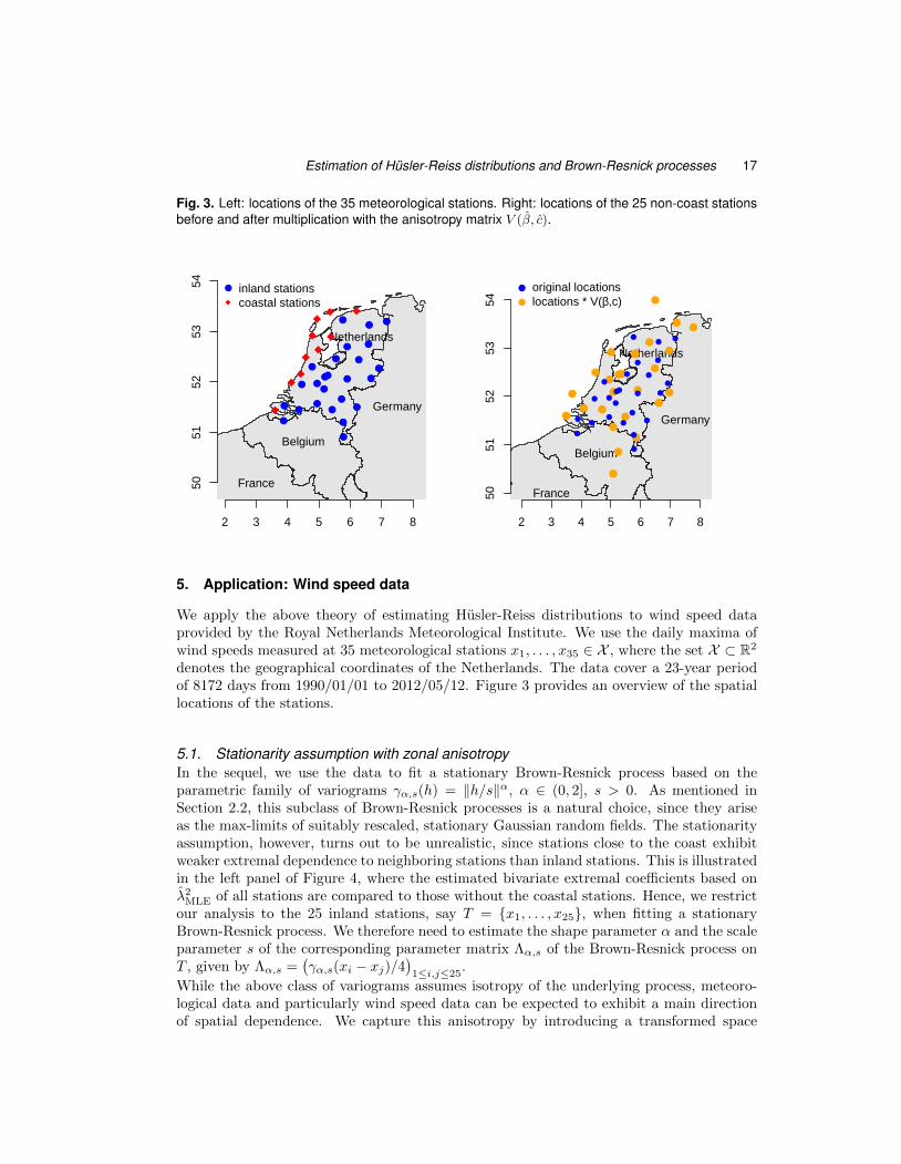
Fig. 3. Left: locations of the 35 meteorological stations. Right: locations of the 25 non-coast stationsbefore and after multiplication with the anisotropy matrix V (β, c).
2 3 4 5 6 7 8
5051
5253
54
Germany
Belgium
France
Netherlands
●
●●
●
●
●
●
●
●
●
●
●
●
●
●●
● ●
●
●
●
●
●
●
●
● inland stationscoastal stations
2 3 4 5 6 7 8
5051
5253
54
Germany
Belgium
France
Netherlands●
●●
●
●
●
●
●
●
●
●
●
●
●
●
●
●●
●
●
●●
●
●
●
●
●●
●
●
●
●
●
●
●
●
●
●
●
●●
● ●
●
●
●
●
●
●
●
●
●
original locationslocations * V(β,c)
5. Application: Wind speed data
We apply the above theory of estimating Husler-Reiss distributions to wind speed dataprovided by the Royal Netherlands Meteorological Institute. We use the daily maxima ofwind speeds measured at 35 meteorological stations x1, . . . , x35 ∈ X , where the set X ⊂ R2
denotes the geographical coordinates of the Netherlands. The data cover a 23-year periodof 8172 days from 1990/01/01 to 2012/05/12. Figure 3 provides an overview of the spatiallocations of the stations.
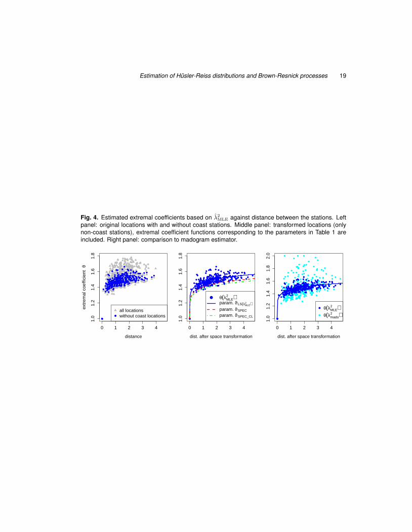
5.1. Stationarity assumption with zonal anisotropyIn the sequel, we use the data to fit a stationary Brown-Resnick process based on theparametric family of variograms γα,s(h) = ‖h/s‖α, α ∈ (0, 2], s > 0. As mentioned inSection 2.2, this subclass of Brown-Resnick processes is a natural choice, since they ariseas the max-limits of suitably rescaled, stationary Gaussian random fields. The stationarityassumption, however, turns out to be unrealistic, since stations close to the coast exhibitweaker extremal dependence to neighboring stations than inland stations. This is illustratedin the left panel of Figure 4, where the estimated bivariate extremal coefficients based onλ2
MLE of all stations are compared to those without the coastal stations. Hence, we restrictour analysis to the 25 inland stations, say T = {x1, . . . , x25}, when fitting a stationaryBrown-Resnick process. We therefore need to estimate the shape parameter α and the scaleparameter s of the corresponding parameter matrix Λα,s of the Brown-Resnick process onT , given by Λα,s =
(γα,s(xi − xj)/4
)1≤i,j≤25
.
While the above class of variograms assumes isotropy of the underlying process, meteoro-logical data and particularly wind speed data can be expected to exhibit a main directionof spatial dependence. We capture this anisotropy by introducing a transformed space
18 S. Engelke, A. Malinowski, Z. Kabluchko, M. Schlather
Table 1. Estimation results. The values for the standard deviation are obtained from simulating andre-estimating the respective models 100 times.
estimator α s β c
ϑPROJ, LS 0.296 (0.0193) 0.234 (0.0744) 0.379 (0.532) 1.67 (0.1761)
ϑSPEC 0.338 (0.0166) 0.687 (0.1797) 0.456 (0.439) 2.21 (0.1596)
ϑSPEC, CL 0.346 (0.0234) 1.025 (0.4806) 0.144 (0.520) 1.61 (0.1846)
X = V X (cf. right panel of Figure 3), where
V = V (β, c) =(
cos β − sin βc sin β c cos β
), β ∈ [0, 2π], c > 0,
is a rotation and dilution matrix; Blanchet and Davison (2011) recently applied this ideato the extremal Gaussian process of Schlather (2002). The new parametric variogrammodel becomes Λϑ =
(γα,s(V xi − V xj)/4
)1≤i,j≤25
, where ϑ = (α, s, β, c) is the vector of
parameters. As in the above simulation study, we apply the three estimators
ϑPROJ, LS = arg minϑ∈Θ
∥∥(λ2MLE,ij)1≤i,j≤25 − Λϑ
∥∥2, ϑSPEC, ϑSPEC, CL. (27)
For all estimators, the data is first normalized as described at the beginning of Section 3and the threshold u(n) is chosen in such a way that, out of the 8172 days, all data above the97.5%-quantile are labeled as extremal. Note that these numbers coincide with the secondset of parameters (n, q(n)) in the simulation study. Hence, the middle row of Figure 1provides a rough estimate of the estimation error.
The estimation results and standard deviations for the parameters (α, s, β, c) are givenin Table 1. The middle panel of Figure 4 illustrates the effect of transforming the space viathe matrix V and displays the fitted extremal coefficient functions for the three estimatorsin (27). Moreover, the right panel shows the estimates of pairwise extremal coefficients
based on λ2MLE and the model-independent madogram estimator, where the latter exhibits
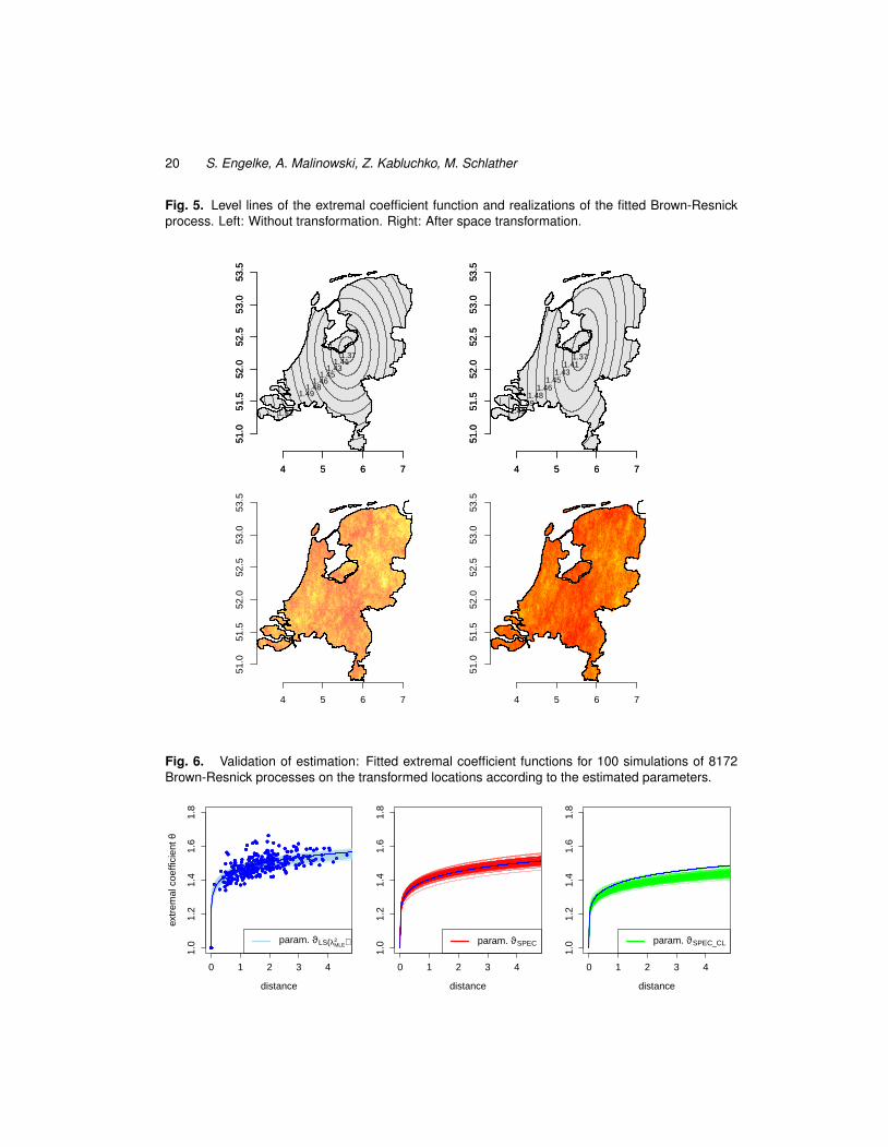
a considerably larger variation. In Figure 5, we illustrate the effect of transforming the spacevia the matrix V (β, c) on the extremal coefficient function and on a typical realization ofthe corresponding Brown-Resnick process.
In order to validate the reliability of the estimated model parameters ϑ, we re-simulatedata in the MDA of the three fitted Brown-Resnick models. Similarly to the simulationstudy, we use 8172 realizations of the Brown-Resnick process itself (which is clearly in its
own MDA) for the daily data. As index set, we use the transformed locations V (β, c)Ton which the Brown-Resnick process is isotropic. Based on this new data, we apply theestimation procedure exactly as for the real data to obtain new estimates for ϑ and thusfor the extremal coefficient function. This is repeated 100 times and the results for thethree different estimators in (27) are shown in Figure 6. In agreement with the results
of the simulation study, the multivariate estimator ϑSPEC seems to be most reliable sincethe re-estimated extremal coefficient functions are close to the true value of the simulation.In contrast, the composite likelihood estimator ϑSPEC, CL significantly underestimates thetrue degree of extremal dependence. This is probably a result of the false assumption ofindependence of bivariate densities which underlies the concept of composite likelihoods.
Estimation of Husler-Reiss distributions and Brown-Resnick processes 19
Fig. 4. Estimated extremal coefficients based on λ2MLE against distance between the stations. Left
panel: original locations with and without coast stations. Middle panel: transformed locations (onlynon-coast stations), extremal coefficient functions corresponding to the parameters in Table 1 areincluded. Right panel: comparison to madogram estimator.
0 1 2 3 4
1.0
1.2
1.4
1.6
1.8
distance
extr
emal
coe
ffici
ent
θ
●
●●
●●
●
●
●
●
●
●
●
●
●
●
●
●
●
●
●
●●
●●
●
●
●
●
●
●
●
●
●
●●●
●
●●
●
●●
●
●
●
●●
●
●
●
●
●
●
●
●
●
● ●●
●●
●
●
●
●
●●
●
●
●
●●
●●
●
●
●
●
●
●
●
●
●● ●
●
●● ●
●
●
●
●
●
●
●●
●●●
●●
●
●
●
●
●●
●
●
●
●
● ●●
●
●●
●
●
●●
●
●●
●
●
●●
●
●
●●
●
●
●●
●
●
●●
●●
●
●
●●
●●
●
●
●
●
●
●
●
●
● ●
●
●
●
●
●
●
●
●
●
●
●
●
●
●
●
●
●
●
●
●
●
●
●
●
●
●
●
●
●
●
●
●
●
●
●
●●
●
●
●
●
●
●
●●
●
●
●
●
●
●
●
●
●
●
●
●
●●
●
●
●
●
●
●
● ●
●
●●
●●
●
●
●
●
●
●
●
●●●
●
●
●
●
●● ●
●
●
●
●
●
●
●
●
●● ●
●
●
●
●
●
●
●
●
●●
●●
●
●●
●
●●
●●
●
●
●●
●
●
●
●
●
●
●
●
●●
●
●
●● ●
●
● ●
●
●
●
●
●
●
●●
●
●
●
●
●
●
●
●●
●●
●● ●
●
●
●
● ●
●
●
●●
●
●
●●
●
●
●
●
●
● ●●
●
●●●●
●
●
●
● ●●●
●
●
●●
●
●
●
●
●
●
●●
●
●
●●
●
●
●
●
●
●
●
●
●
●
●
●●
●
●
●
●
●
●
●
●●
●
● ●●
●
●
●
●
● ● ●●
●
●
●
●
●
●
●
●
●
●
●
●
●
●
●●
● ●
●
●●
●●
●●
●
●
●
●
●●
●
●●
●
●
●
●
●
● ●
●●
●
●
●
●
●
●
●
●●
●
●
●
●
●
●
●
●
●●
●
● ●
●
● ●●
●
●
●●
●
●●
●
●
●
●
●
●
●
●
●●
●
●
●
●
●
●●●
●
●
●
●
●
●
●●
●
●
●
●
●●
●
●
●
●
●●
●
●
●
●
●
●
●
●
●
●
●
●●
●
●
●
●
●
●
●
●
●
●
●
●
●
●
●●
●
●
●●
●●
●
●
● ● ●●
●
● ●
●
●
●●●
●
●
●
●
● ●
●
●
●
●
●
●●
●
● ●
●
●
●
●
●●
●
●●
●●●
●
●
●
●
●
●
●
●
●
●●
●
●
●
●
●
●
●
●
●
●
●●
●●
●
●
●
●
all locationswithout coast locations
●
●●
●●
●
●
●
●
●
●
●
●
●
●
●
●
●
●
●
●●
●●
●
●
●
●
●
●
●
●
●
●●●
●
●●
●
●●
●
●
●
●●
●
●
●
●
●
●
●
●
●
● ●●
●●
●
●
●
●
●●
●
●
●
●●
●●
●
●
●
●
●
●
●
●
●● ●
●
●● ●
●
●
●
●
●
●
●●
●●●
● ●
●
●
●
●
●●
●
●
●
●
● ●●
●
●●
●
●
●●
●
●●
●
●
●●
●
●
●●
●
●
●●
●
●
●●
●●
●
●
●●
●●
●
●
●
●
●
●
●
●
● ●
●
●
●
●
●
●
●
●
●
●
●
●
●
●
●
●
●
●
●
●
●
●
●
●
●
●
●
●
●
●
●
●
●
●
●
●●
●
●
●
●
●
●
●●
●
●
●
●
●
●
●
●
●
●
●
●
●●
●
●
●
●
●
●
● ●
●
●●
●●
●
●
●
●
●
●
●
●●●
●
●
●
●
●● ●
●
●
●
●
●
●
●
●
●● ●
●
●
●
●
●
●
●
●
● ●
●●
●
●●
●
●●
●●
●
●
●●
●
●
●
●
●
●
●
●
●●
●
●
●● ●
●
●●
●
●
●
●
●
●
●●
●
●
●
●
●
●
●
●●
●●
●● ●
●
●
●
● ●
●
●
●●
●
●
●●
●
●
●
●
●
● ●●
●
●●
●●
●
●
●
● ●●●
●
●
●●
●
●
●
●
●
●
●●
●
●
●●
●
●
●
●
●
●
●
●
●
●
●
●●
●
●
●
●
●
●
●
●●
●
● ●●
●
●
●
●
● ● ●●
●
●
●
●
●
●
●
●
●
●
●
●
●
●
●●
● ●
●
●●
●●
●●
●
●
●
●
●●
●
●●
●
●
●
●
●
●●
●●
●
●
●
●
●
●
●
●●
●
●
●
●
●
●
●
●
●●
●
●●
●
● ●●
●
●
●●
●
●●
●
●
●
●
●
●
●
●
●●
●
●
●
●
●
●●
●
●
●
●
●
●
●
●●
●
●
●
●
●●
●
●
●
●
● ●
●
●
●
●
●
●
●
●
●
●
●
●●
●
●
●
●
●
●
●
●
●
●
●
●
●
●
●●
●
●
●●
●●
●
●
● ● ●●
●
●●
●
●
●●●
●
●
●
●
● ●
●
●
●
●
●
●●
●
● ●
●
●
●
●
●●
●
●●
●●●
●
●
●
●
●
●
●
●
●
●●
●
●
●
●
●
●
●
●
●
●
●●
●●
●
●
●
0 1 2 3 4
1.0
1.2
1.4
1.6
1.8
dist. after space transformation
● θ(λMLE2 )
param. ϑLS(λMLE2 )
param. ϑSPEC
param. ϑSPEC_CL●
●
●
● ●
●
●
●
●
●
●
●
●
●
●
●
●
●
●
●
●●
●
●
●●
●
●
●
●
●
●
●
●●
●
●
●
●
●
●
●
●
●
●
●●
●
●
●
●
●
●
●
●
●●
●
●●
●
●
●
●
●
●
●
●
●
●●
●
●
●
●
●
●
●
●
●
●●
●
●
●
●
●
●
●
●
●
●
●
●
●
●
●
●
●
●
●
●
●
●
●
●
●
●
●
●
●
●
●
●●
●
●●
●
●
●
● ●
●
●
●
●
●
●
●
●
●
●
●
●
●
●
●
●
●
●
●
●
●
●
●●
●
●
●
●
●
●
●
●
●
●
●●
●
●
●
●
●
●
●
●
●
●
● ●
●
●
●
●
●
●●
●
●
●
●
●
●
●
●
●
●
●
●
●
●
●
●
●
●
●
●
●
●
●
●
●
●
●
● ●
●
●
●
●
●
●
●
●
●
●
●
●
● ●
●
●
●
●
●●
●
●●
●
●
●
●
●
●
●
●●
●
●
●
●
●
●
●●
●
●
●
●
●
●
●
●
●
●
●
●
●
●
●
●
●
●
●
●
●
●
●
●●
●●
●
●
●
●
●
●
●
●
●
●
●
●
●
●
●
●
●
●
●
●
●
●
●
●
●
●
●
●
●
●
●
●
●●
●
●
●
●
●
●
●
●
●
●
●●
●
●
●
●
●
●
●
●●
●
●
●
●
●●
●
●
●
●
●●
●
●
●
●●
●●
●
●
●
●
●
●●
●●
●
●
●
●
●
●
●
●
●
●●
●
●
●
●
●
●
●
●
●
●
●
●
●
●
● ●
●
●
●
●
●
●
●
●
●
●
●● ●
●
●
●
●
●
●
●
●
●
●
●
●
●
●
●
●
●●
●
●
●
●
●
●
● ●
●
●
●
●
●
●
●
●
●
●
●
●
●
●
●
●
●●
●
●
●
●
●●
●
●
●
●
●●
●
●
●
●
●
●
●
●
●
●
●
●
●
●
●
●
●
●
●
●
●
●
●●
●
●
●
●●
●
●
●
●
●
●
●
●
●
●
●
●
●
●
●
●
●
●
●
●
●
●
●
●
●
●●
●
●
●
●●
●
●
●
●
●
●
●
●
●
●
●
●
●
●
●
●
●
●
●●
●
●
●
●
●
●
●
●
●
●
●
●
●
●
●
●
●
●
●
●
●
●
●
● ●
●
●
●
●
●
●
●
●
●
●
●
● ●
●
●
●
●●
●
●
●
●
●
●
●●
●
●
●
●
●
● ●
●
●
●
●●
●
●
●
●
●
●
●
●
●
●●
●
●
●
●
●
●
●
●
●
●
●
●
●●
●●
●
0 1 2 3 4
1.0
1.2
1.4
1.6
1.8
2.0
dist. after space transformation
●
●●
●●
●
●
●
●
●
●
●
●
●
●
●
●
●
●
●
●●
●●
●
●
●
●
●
●
●
●
●
●●●
●
●●
●
●●
●●
●
●●
●
●
●
●
●
●
●
●
●
● ●●
●●
●
●
●
●
●●
●
●
●
●●
●●
●
●
●
●
●
●
●
●
●● ●
●●● ●
●
●
●
●
●
●
●●
●●●
● ●
●
●
●
●
●●
●
●
●
●
● ●●
●
●●
●
●
●●
●
●●
●
●
●●
●
●
●●
●●
●●
●
●
●●
●●
●
●
●●
●●
●
●
●
●
●
●
●
●
● ●
●
●
●
●
●
●
●
●
●
●
●●
●
●
●
●
●
●●
●
●
●
●
●
●
●
●
●
●
●
●
●
●
●
●
●●
●
●
●
●
●
●
●●
●
●
●
●
●
●
●●
●
●
●
●
●●
●
●
●●
●●
● ●
●
●●
●●
●
●
●
●
●
●
●
●●●
●●
●
●
●● ●●
●
●
●
●
●
●
●
●● ●
●
●
●
●
●
●
●
●
● ●
●●●
●●
●
●●
●●
●
●
●●
●
●
●
●
●
●●
●
●●
●
●
●● ● ●
●●
●
●
●●
●
●
●●
●
●
●
●
●
●
●
●●
●●
●● ●
●
●
●
● ●
●●
●●
●
●●●
●
●
●
●
●
● ●●
●
●●
●●
●
●
●
● ● ●●
●
●
●●
●
●
●
●
●
●
●●
●
●
●●
●●
●
●
●
●
●
●
●
●
●
● ●●
●
●
●
●
●
●
●●
●
● ●●
●
●
●
●
● ● ●●
●
●
●●
●
●
●
●
●
●
●
●
●
●
●●
● ●
●
●●
●●
●●●
●
●
●
●●
●
●●
●
●
●
●
●
●●●
●
●
●
●
●
●
●
●●
●●
●
●
●
●
●
●
●
●●
●
●●●
● ●●
●
●
●●
●
●●
●
●●
●●
●
●●
●●
●
●
●
●
●
● ●●
●
●
●
●
●
●
●●
●
●
●
●
●●
●
●
●
●
● ●
●
●
●
●
●
●
●
●
●
●
●
●●
●
●
●
●
●●
●
●
●
●
●
●
●
●
● ●
●
●
●●
●●
●
●
● ● ●●
●
●●
●
●
●●●
●
●
●
●
● ●
●
●
●
●
●
●●
●
● ●
●
●
●
●
●●
●
●●
●●●
●
●
●
●
●
●
●
●
●
●●
●
●
●
●
●
●
●
●
●
●
●●
●●
●
●
●
●
●
θ(λMLE2 )
θ(λmado2 )
20 S. Engelke, A. Malinowski, Z. Kabluchko, M. Schlather
Fig. 5. Level lines of the extremal coefficient function and realizations of the fitted Brown-Resnickprocess. Left: Without transformation. Right: After space transformation.
4 5 6 7
51.0
51.5
52.0
52.5
53.0
53.5
1.371.41
1.431.45
1.461.48
1.49
1.51
4 5 6 7
51.0
51.5
52.0
52.5
53.0
53.5
4 5 6 751
.051
.552
.052
.553
.053
.5
1.371.41
1.431.45
1.461.48
1.491.49
4 5 6 751
.051
.552
.052
.553
.053
.5
4 5 6 7
51.0
51.5
52.0
52.5
53.0
53.5
●●●●●●●
●●●●●●●●●●
●●●●●●●●●●●●●●
●●●●●●●●●●●●
●●●●●●●●●●●●
●●●●●●●●●●●●●●
●●●●●●●●●●●●●●●●●●
●●●●●●●●●●●●●●●●
●
●●●●●●●●●●●●●●●●●●●●
●●●●●
●●●●●●●●●●●●●●●●●●●●●●●●●●●●●●●●●●●●●
●●●●●●●●●●●●●●●●●●●●●●●●●●●●●●●●●●●●●●
●●●●●●●●●●●●●●●●●●●●●●●●●●●●●●●●●●●●●●●
●●●●●●●●●●●●●●●●●●●●●●●●●●●●●●●●●●●●●●
●●●●●●●●●●●●●●●●●●●●●●●●●●●●●●●●
●
●●●●●●●●●●●●●●●●●●●●●
●●●●●●●●●●●●●●●●●●●●●
●●●●●●
●●●●●●●●●●●●●●●●●●
●●●●●●●●●●●●●
●●●●●●●●●●●●●●●●●
●●●●●●●●●●●●●●●●●●
●●●●●●●●●●●●●●●●●●
●●●●●●●●●●●●●●●●●●●●●●●●●●●●●●●
●●●●●●●●●●●●●●●●●●
●●●●●●●●●●●●●●●●●●●●●●●●●●●●●●●●●●
●●●●●●●●●●●●●●●●●
●●●●●●●●●●●●●●●●●●●●●●●●●●●●●●●●●●●
●●●●●●●●●●●●●●●●●
●●●●●●●●●●●●●●●●●●●●●●●●●●●●●●●●●●
●●●●●●●●●●●●●●●●●
●●●●●●●●●●●●●●●●●●●●●●●●●●●●●●●●●●
●●●●●●●●●●●●●●●●●●
●●●●●●●●●●●●●●●●●●●●●●●●●●●●●●●●
●●●
●●●●●●●
●●●●●●●●●●●●●●●●●●●●●●●●●●●●●●●
●●●●●
●●●●●●●●●●●●●●●●●●●●●●●●●●●●●●
●●●●●
●
●●●●●●●●●●●●●●●●●●●●●●●●●●●●●●●●●●●●●●●●●
●●
●●●
●●●●●●●●●●●●●●●●●●●●●●●●●●●●●●●●●●●●●●●●●
●●●●●
●●●●●●●●●●●●●●●●●●●●●●●●●●●●●●●●●●●●●●●
●●
●●●●●●●●●●●●●●
●●●●●●●●●●●●●●●●●●●●●●●●●●
●●●●●●●●●●●●
●●●●●●●●●●●●●●●●●●
●●●●●●●●●●
●●●●●●●●●
●●●●●●●●●●●●●●●●●
●●●●●●●●●●●●●●●●●●●●●
●●●●●●●
●●●●●●●●●●●●●●●●
●●●●●●●●●●●●●●●●●●●●●●●●
●
●●●●●●●●●●●●●●
●●●●●●●●●●●●●●●●●●●●●●●●●●
●●●
●●●●●●●●●●●
●●●●●●●●●●●●●●●●●●●●●●●●●●●
●●●●●●
●●●●●●●●●
●●●●●●●●●
●●●●●●●●●●●●●●●●●●●●●●●●●
●●●●●●●
●●●●●●●●●●●●●●●
●●●●●●●●●
●●●●●●●●●●●●●●●●●●●●●●
●●●●●●●●
●●●●●●●●●●●●●●●●●●●●●●●●●
●●●●●●●●●●●
●●●●●●●●●●●●●●●●●●●●●●●
●●●●●●●●●●●●●●●●●●●●●●●●●●●●●●●●●●●●●●●●●●●●●●●●●●●●●●●●
●●●●●●●●●●●●●●●●●●●●●●●
●●●●●●●●●●●●●●●●●●●●●●●●●●●●●●●●●●●●●●●●●●●●●●●●●●●●●●
●●●●●●●●●●●●●●●●●●●●●
●●●●●●●●●●●●●●●●●●●●●●●●
●●●●●●●●●●●●●●●●●●●●●●●●●●●●
●●●
●●●●●●●●●●●●●●●●●●●●●●●●
●●●●●●●●●●●●●●●●●●●●●
●●●●
●●●●●●●●●●●●●●●●●●●●●●●
●●●●●●●
●●●●●●●●●●●●●●●●●●●●●●●●●●●
●●●●●●●●●●●●●●●●●●●●●●●●●
●●●●●●●●●●●●●●●●●●●●●●●●●●●●●●●●●●●●●
●●●●●●●●●●●●●●●●●●●●●●●●●●
●●●●●●●
●●●●●●●●●●●●●●●●●●●●●●●●●●●●●●●●●●●●●●●●●●●●●●●●●●●
●●●●●●●●●●●●●●●●●●●●●●●●●●
●
●●●●●●●●●●●●●●●●●●●●●●●●●●●●●●●●●●●●●●●●●●●●●●●
●●●●●●●●●●●●●●●●●●●●●●●●●
●●●●●●●●●●●●●●●●●●●●●●●●●●●●●●●●●●●●●●●●●●●●●●
●●●
●●●●●●●●●●●●●●●●●●●●
●●●●
●●
●●●●
●●●●●●●●●●●●●●●●●●●●●●●●●●●●●●●●●●●●●●●●●●●●●
●●
●●●●●●●●●●●●●●●●●●
●●●●●●
●●●●●●●●●●●●●●●●●●●●●●●●●●●●●●●●●●●●●●●●●●●●●●●●●●●●●●●●
●●●●
●●●
●●●●●●●●
●●●
●●●●●
●●●●●●●●●●●●●●●●●●●●●●●●●●●●●●●●●●●●●●●●●●●●●●●●●●●●●●●●●●
●●●●●●●●●
●●●
●●●●●●
●●●●●
●●
●●●●●●●●●●●●●●●●●●●●●●●●●●●●●●●●●●●●●●●●●●●●●●●●●●●●●●●●●●●●●●●●●●●
●●●●●●●●●●
●●●●●●●●●●●●●●●
●●●●●
●●●●●●●●●●●●●●●●●●●●●●●●●●●●●●●●●●●●●●●●●●●●●●●●●●●●●●●●●●●●●●●●●●●●●
●●●●●●●●●●●
●●●●●●●●●●●●●●●●●●●●●●●
●●●●●●●●●●●
●●●●●●●●●●●●●●●●●●●●●●●●●●●●●●●●●●●●●●●●●●●●●●●●●●●●●●●●●●●●●●●●●●●●●●●●●●●●●●●●●●●●●●
●●●●●●●●●●●●●●●●●●●●●●●●●●●●
●●●●●●●●●●●
●●●●●●●●●●●●●●●●●●●●●●●●●●●●●●●●●●●●●●●●●●●●●●●●●●●●●●●●●●●●●●●●●●●●●●●●●●●●●●●●●●●
●●●●●●●●●●●●●●●●●●●●●●●●●●●●●
●
●●●●●●●●●●●●●
●●●●●●●●●●●●●●●●●●●●●●●●●●●●●●●●●●●●●●●●●●●●●●●●●●●●●●●●●●●●●●●●●●●●●●●●●●●●●●●
●●●●●●●●●●●●●●●●●●●●●●●●●●●●●●
●●●●●●●●●●●
●●●●●●●●●●●●●
●●●●●●●●●●●●●●●●●●●●●●●●●●●●●●●●●●●●●●●●●●●●●●●●●●●●●●●●●●●●●●●●●●●●●●●●●●●●●●●
●●●●●●●●●●●●●●●●●●●●●●●●●●●●●●●●
●●●●●●●●●●●●●●
●●
●●●●●●●●●●●●
●●●●●●●●●●●●●●●●●●●●●●●●●●●●●●●●●●●●●●●●●●●●●●●●●●●●●●●●●●●●●●●●●●●●●●●●●●●●●●●●●●●●
●●●●●●●●●●●●●●●●●●●●●●●●●●●●●●●●●●●●●●●●●●●●●●●●●●●●●●●●●●
●●●●●●●●●●●●●●
●●●●●●●●●●●●●●●●●●●●●●●●●●●●●●●●●●●●●●●●●●●●●●●●●●●●●●●●●●●●●●●●●●●●●●●●●●●●●●●●●●●●●●●●●●●●●●●●●●●●●●●●●●●●●●●●●●●●●●●●●●●●●●●●●●●●●●●●●●●●●●●●●●●●●●●●●●●●●●●●●●●●●●●●
●●●●●●●●●●●●●●●●●●●●●●●●●●●●●●●●●●●●●●●●●●●●●●●●●●●●●●●●●●●●●●●●●●●●●●●●●●●●●●●●●●●●●●●●●●●●●●●●●●●●●●●●●●●●●●●●●●●●●●●●●●●●●●●●●●●●●●●●●●●●●●●●●●●●●●●●●●●●●●●●●●●●●●●
●●●●●●●●●●●●●●●●●●●●●●●●●●●●●●●●●●●●●●●●●●●●●●●●●●●●●●●●●●●●●●●●●●●●●●●●●●●●●●●●●●●●●●●●●●●●●●●●●●●●●●●●●●●●●●●●●●●●●●●●●●●●●●●●●●●●●●●●●●●●●●●●●●●●●●●●●●●●●●●●●●●●●●●●●
●●●●●●●●●●●●●●●●●●●●●●●●●●●●●●●●●●●●●●●●●●●●●●●●●●●●●●●●●●●●●●●●●●●●●●●●●●●●●●●●●●●●●●●●●●●●●●●●●●●●●●●●●●●●●●●●●●●●●●●●●●●●●●●●●●●●●●●●●●●●●●●●●●●●●●●●●●●●●●●●●●●●●●●●●●●●
●●●●●●●●●●●●●●●●●●●●●●●●●●●●●●●●●●●●●●●●●●●●●●●●●●●●●●●●●●●●●●●●●●●●●●●●●●●●●●●●●●●●●●●●●●●●●●●●●●●●●●●●●●●●●●●●●●●●●●●●●●●●●●●●●●●●●●●●●●●●●●●●●●●●●●●●●●●●●●●●●●●●●●●●●●●●●●
●●●●●●●●●●●●●●●●●●●●●●●●●●●●●●●●●●●●●●●●●●●●●●●●●●●●●●●●●●●●●●●●●●●●●●●●●●●●●●●●●●●●●●●●●●●●●●●●●●●●●●●●●●●●●●●●●●●●●●●●●●●●●●●●●●●●●●●●●●●●●●●●●●●●●●●●●●●●●●●●●●●●●●●●●●●●●●●●●
●●●●●●●●●●●●●●●●●●●●●●●●●●●●●●●●●●●●●●●●●●●●●●●●●●●●●●●●●●●●●●●●●●●●●●●●●●●●●●●●●●●●●●●●●●●●●●●●●●●●●●●●●●●●●●●●●●●●●●●●●●●●●●●●●●●●●●●●●●●●●●●●●●●●●●●●●●●●●●●●●●●●●●●●●●●●●●●
●●●●●●●●●●●●●●●●●●●●●●●●●●●●●●●●●●●●●●●●●●●●●●●●●●●●●●●●●●●●●●●●●●●●●●●●●●●●●●●●●●●●●●●●●●●●●●●●●●●●●●●●●●●●●●●●●●●●●●●●●●●●●●●●●●●●●●●●●●●●●●●●●●●●●●●●●●●●●●●●●●●●●●●●●●●
●●●●●●●●●●●●●●●●●●●●●●●●●●●●●●●●●●●●●●●●●●●●●●●●●●●●●●●●●●●●●●●●●●●●●●●●●●●●●●●●●●●●●●●●●●●●●●●●●●●●●●●●●●●●●●●●●●●●●●●●●●●●●●●●●●●●●●●●●●●●●●●●●●●●●●●●●●●●●●●●●●●
●●
●●●●●●●●●●●●●●●●●●●●●●●●●●●●●●●●●●●●●●●●●●●●●●●●●●●●●●●●●●●●●●●●●●●●●●●●●●●●●●●●●●●●●●●●●●●●●●●●●●●●●●●●●●●●●●●●●●●●●●●●●●●●●●●●●●●●●●●●●●●●●●●●●●●●●●●●●●●●●●●●●●
●●
●●●●●●●●●●●●●●●●●●●●●●●●●●●●●●●●●●●●●●●●●●●●●●●●●●●●●●●●●●●●●●●●●●●●●●●●●●●●●●●●●●●●●●●●●●●●●●●●●●●●●●●●●●●●●●●●●●●●●●●●●●●●●●●●●●●●●●●●●●●●●●●●●●●●●●●●●●●●●●●●
●●●●●●●●●●●●●●●●●●●●●●●●●●●●●●●●●●●●●●●●●●●●●●●●●●●●●●●●●●●●●●●●●●●●●●●●●●●●●●●●●●●●●●●●●●●●●●●●●●●●●●●●●●●●●●●●●●●●●●●●●●●●●●●●●●●●●●●●●●●●●●●●●●●●●●●●●●●●●●●●●
●●●●●●●●●●●●●●●●●●●●●●●●●●●●●●●●●●●●●●●●●●●●●●●●●●●●●●●●●●●●●●●●●●●●●●●●●●●●●●●●●●●●●●●●●●●●●●●●●●●●●●●●●●●●●●●●●●●●●●●●●●●●●●●●●●●●●●●●●●●●●●●●●●●●●●●●●●●●●●●●●●
●●●●●●●●●●●●●●●●●●●●●●●●●●●●●●●●●●●●●●●●●●●●●●●●●●●●●●●●●●●●●●●●●●●●●●●●●●●●●●●●●●●●●●●●●●●●●●●●●●●●●●●●●●●●●●●●●●●●●●●●●●●●●●●●●●●●●●●●●●●●●●●●●●●●●●●●●●●●●●●●●
●●●●●●●●●●●●●●●●●●●●●●●●●●●●●●●●●●●●●●●●●●●●●●●●●●●●●●●●●●●●●●●●●●●●●●●●●●●●●●●●●●●●●●●●●●●●●●●●●●●●●●●●●●●●●●●●●●●●●●●●●●●●●●●●●●●●●●●●●●●●●●●●●●●●●●●●●●●●●●●●●
●●●●●●●●●●●●●●●●●●●●●●●●●●●●●●●●●●●●●●●●●●●●●●●●●●●●●●●●●●●●●●●●●●●●●●●●●●●●●●●●●●●●●●●●●●●●●●●●●●●●●●●●●●●●●●●●●●●●●●●●●●●●●●●●●●●●●●●●●●●●●●●●●●●●●●●●●●●●●●●●●
●●●●●●●●●●●●●●●●●●●●●●●●●●●●●●●●●●●●●●●●●●●●●●●●●●●●●●●●●●●●●●●●●●●●●●●●●●●●●●●●●●●●●●●●●●●●●●●●●●●●●●●●●●●●●●●●●●●●●●●●●●●●●●●●●●●●●●●●●●●●●●●●●●●●●●●●●●●●●●●●●
●●●●●●●●●●●●●●●●●●●●●●●●●●●●●●●●●●●●●●●●●●●●●●●●●●●●●●●●●●●●●●●●●●●●●●●●●●●●●●●●●●●●●●●●●●●●●●●●●●●●●●●●●●●●●●●●●●●●●●●●●●●●●●●●●●●●●●●●●●●●●●●●●●●●●●●●●●●●●●●●
●●●●●●●●●●●●●●●●●●●●●●●●●●●●●●●●●●●●●●●●●●●●●●●●●●●●●●●●●●●●●●●●●●●●●●●●●●●●●●●●●●●●●●●●●●●●●●●●●●●●●●●●●●●●●●●●●●●●●●●●●●●●●●●●●●●●●●●●●●●●●●●●●●●●●●●●●●●●●●●●
●●●●●●●●●●●●●●●●●●●●●●●●●●●●●●●●●●●●●●●●●●●●●●●●●●●●●●●●●●●●●●●●●●●●●●●●●●●●●●●●●●●●●●●●●●●●●●●●●●●●●●●●●●●●●●●●●●●●●●●●●●●●●●●●●●●●●●●●●●●●●●●●●●●●●●●●●●●●●●●●●
●●●●●●●●●●●●●●●●●●●●●●●●●●●●●●●●●●●●●●●●●●●●●●●●●●●●●●●●●●●●●●●●●●●●●●●●●●●●●●●●●●●●●●●●●●●●●●●●●●●●●●●●●●●●●●●●●●●●●●●●●●●●●●●●●●●●●●●●●●●●●●●●●●●●●●●●●●●●●●●●●
●●●●●●●●●●●●●●●●●●●●●●●●●●●●●●●●●●●●●●●●●●●●●●●●●●●●●●●●●●●●●●●●●●●●●●●●●●●●●●●●●●●●●●●●●●●●●●●●●●●●●●●●●●●●●●●●●●●●●●●●●●●●●●●●●●●●●●●●●●●●●●●●●●●●●●●●●●●●●●●●●
●●●●●●●●●●●●●●●●●●●●●●●●●●●●●●●●●●●●●●●●●●●●●●●●●●●●●●●●●●●●●●●●●●●●●●●●●●●●●●●●●●●●●●●●●●●●●●●●●●●●●●●●●●●●●●●●●●●●●●●●●●●●●●●●●●●●●●●●●●●●●●●●●●●●●●●●●●●●●●●●
●●●●●●●●●●●●●●●●●●●●●●●●●●●●●●●●●●●●●●●●●●●●●●●●●●●●●●●●●●●●●●●●●●●●●●●●●●●●●●●●●●●●●●●●●●●●●●●●●●●●●●●●●●●●●●●●●●●●●●●●●●●●●●●●●●●●●●●●●●●●●●●●●●●●●●●●●●●●●●
●●●●●●●●●●●●●●●●●●●●●●●●●●●●●●●●●●●●●●●●●●●●●●●●●●●●●●●●●●●●●●●●●●●●●●●●●●●●●●●●●●●●●●●●●●●●●●●●●●●●●●●●●●●●●●●●●●●●●●●●●●●●●●●●●●●●●●●●●●●●●●●●●●●●●●●●●●●●●
●●●●●●●●●●●●●●●●●●●●●●●●●●●●●●●●●●●●●●●●●●●●●●●●●●●●●●●●●●●●●●●●●●●●●●●●●●●●●●●●●●●●●●●●●●●●●●●●●●●●●●●●●●●●●●●●●●●●●●●●●●●●●●●●●●●●●●●●●●●●●●●●●●●●●●●●●●●●
●●●●●●●●●●●●●●●●●●●●●●●●●●●●●●●●●●●●●●●●●●●●●●●●●●●●●●●●●●●●●●●●●●●●●●●●●●●●●●●●●●●●●●●●●●●●●●●●●●●●●●●●●●●●●●●●●●●●●●●●●●●●●●●●●●●●●●●●●●●●●●●●●●●●●●●●●●●
●●●●●●●●●●●●●●●●●●●●●●●●●●●●●●●●●●●●●●●●●●●●●●●●●●●●●●●●●●●●●●●●●●●●●●●●●●●●●●●●●●●●●●●●●●●●●●●●●●●●●●●●●●●●●●●●●●●●●●●●●●●●●●●●●●●●●●●●●●●●●●●●●●●●●●●●●●
●●●●●●●●●●●●●●●●●●●●●●●●●●●●●●●●●●●●●●●●●●●●●●●●●●●●●●●●●●●●●●●●●●●●●●●●●●●●●●●●●●●●●●●●●●●●●●●●●●●●●●●●●●●●●●●●●●●●●●●●●●●●●●●●●●●●●●●●●●●●●●●●●●●●●●●●●
●●●●●●●●●●●●●●●●●●●●●●●●●●●●●●●●●●●●●●●●●●●●●●●●●●●●●●●●●●●●●●●●●●●●●●●●●●●●●●●●●●●●●●●●●●●●●●●●●●●●●●●●●●●●●●●●●●●●●●●●●●●●●●●●●●●●●●●●●●●●●●●●●●●●●●●
●●●●●●●●●●●●●●●●●●●●●●●●●●●●●●●●●●●●●●●●●●●●●●●●●●●●●●●●●●●●●●●●●●●●●●●●●●●●●●●●●●●●●●●●●●●●●●●●●●●●●●●●●●●●●●●●●●●●●●●●●●●●●●●●●●●●●●●●●●●●●●●●●●●●●●
●●●●●●●●●●●●●●●●●●●●●●●●●●●●●●●●●●●●●●●●●●●●●●●●●●●●●●●●●●●●●●●●●●●●●●●●●●●●●●●●●●●●●●●●●●●●●●●●●●●●●●●●●●●●●●●●●●●●●●●●●●●●●●●●●●●●●●●●●●●●●●●●●●●●
●●●●●●●●●●●●●●●●●●●●●●●●●●●●●●●●●●●●●●●●●●●●●●●●●●●●●●●●●●●●●●●●●●●●●●●●●●●●●●●●●●●●●●●●●●●●●●●●●●●●●●●●●●●●●●●●●●●●●●●●●●●●●●●●●●●●●●●●●●●●●●●●●
●●●●●●●●●●●●●●●●●●●●●●●●●●●●●●●●●●●●●●●●●●●●●●●●●●●●●●●●●●●●●●●●●●●●●●●●●●●●●●●●●●●●●●●●●●●●●●●●●●●●●●●●●●●●●●●●●●●●●●●●●●●●●●●●●●●●●●●●●●●●●
●●●●●●●●●●●●●●●●●●●●●●●●●●●●●●●●●●●●●●●●●●●●●●●●●●●●●●●●●●●●●●●●●●●●●●●●●●●●●●●●●●●●●●●●●●●●●●●●●●●●●●●●●●●●●●●●●●●●●●●●●●●●●●●●●●●●●●●●●
●●●●●●●●●●●●●●●●●●●●●●●●●●●●●●●●●●●●●●●●●●●●●●●●●●●●●●●●●●●●●●●●●●●●●●●●●●●●●●●●●●●●●●●●●●●●●●●●●●●●●●●●●●●●●●●●●●●●●●●●●●●●●●●●●●●●●●●●●
●●●●●●●●●●●●●●●●●●●●●●●●●●●●●●●●●●●●●●●●●●●●●●●●●●●●●●●●●●●●●●●●●●●●●●●●●●●●●●●●●●●●●●●●●●●●●●●●●●●●●●●●●●●●●●●●●●●●●●●●●●●●●●●●●●●●●●●●●
●●●●●●●●●●●●●●●●●●●●●●●●●●●●●●●●●●●●●●●●●●●●●●●●●●●●●●●●●●●●●●●●●●●●●●●●●●●●●●●●●●●●●●●●●●●●●●●●●●●●●●●●●●●●●●●●●●●●●●●●●●●●●●●●●●
●●
●●●●●●●●●●●●●●●●●●●●●●●●●●●●●●●●●●●●●●●●●●●●●●●●●●●●●●●●●●●●●●●●●●●●●●●●●●●●●●●●●●●●●●●●●●●●●●●●●●●●●●●●●●●●●●●●●●●●●●●●●●●●●●●●●
●●●●●●●●●●●●●●●●●●●●●●●●●●●●●●●●●●●●●●●●●●●●●●●●●●●●●●●●●●●●●●●●●●●●●●●●●●●●●●●●●●●●●●●●●●●●●●●●●●●●●●●●●●●●●●●●●●●●●●●●●●●●●●●●
●●●●●●●●●●●●●●●●●●●●●●●●●●●●●●●●●●●●●●●●●●●●●●●●●●●●●●●●●●●●●●●●●●●●●●●●●●●●●●●●●●●●●●●●●●●●●●●●●●●●●●●●●●●●●●●●●●●●●●●●●●●
●●●●●●●●●●●●●●●●●●●●●●●●●●●●●●●●●●●●●●●●●●●●●●●●●●●●●●●●●●●●●●●●●●●●●●●●●●●●●●●●●●●●●●●●●●●●●●●●●●●●●●●●●●●●●●●●●●●●●●●●●●●●
●●●●●●●●●●●●●●●●●●●●●●●●●●●●●●●●●●●●●●●●●●●●●●●●●●●●●●●●●●●●●●●●●●●●●●●●●●●●●●●●●●●●●●●●●●●●●●●●●●●●●●●●●●●●●●●●●●●●●●●●●●
●●●●●●●●●●●●●●●●●●●●●●●●●●●●●●●●●●●●●●●●●●●●●●●●●●●●●●●●●●●●●●●●●●●●●●●●●●●●●●●●●●●●●●●●●●●●●●●●●●●●●●●●●●●●●●●●●●●●●●●●
●●●●●●●●●●●●●●●●●●●●●●●●●●●●●●●●●●●●●●●●●●●●●●●●●●●●●●●●●●●●●●●●●●●●●●●●●●●●●●●●●●●●●●●●●●●●●●●●●●●●●●●●●●●●●●●●●●●●●●●
●●●●●●●●●●●●●●●●●●●●●●●●●●●●●●●●●●●●●●●●●●●●●●●●●●●●●●●●●●●●●●●●●●●●●●●●●●●●●●●●●●●●●●●●●●●●●●●●●●●●●●●●●●●●●●●●●●●●●●●
●●●●●●●●●●●●●●●●●●●●●●●●●●●●●●●●●●●●●●●●●●●●●●●●●●●●●●●●●●●●●●●●●●●●●●●●●●●●●●●●●●●●●●●●●●●●●●●●●●●●●●●●●●●●●●●●●●●●●●●●●●
●●●●●●●●●●●●●●●●●●●●●●●●●●●●●●●●●●●●●●●●●●●●●●●●●●●●●●●●●●●●●●●●●●●●●●●●●●●●●●●●●●●●●●●●●●●●●●●●●●●●●●●●●●●●●●●●●●●●●●●●●●
●●●●●●●●●●●●●●●●●●●●●●●●●●●●●●●●●●●●●●●●●●●●●●●●●●●●●●●●●●●●●●●●●●●●●●●●●●●●●●●●●●●●●●●●●●●●●●●●●●●●●●●●●●●●●●●●●●●●●●●●●●●
●●●●●●●●●●●●●●●●●●●●●●●●●●●●●●●●●●●●●●●●●●●●●●●●●●●●●●●●●●●●●●●●●●●●●●●●●●●●●●●●●●●●●●●●●●●●●●●●●●●●●●●●●●●●●●●●●●●●●●●●●●●●
●●●●●●●●●●●●●●●●●●●●●●●●●●●●●●●●●●●●●●●●●●●●●●●●●●●●●●●●●●●●●●●●●●●●●●●●●●●●●●●●●●●●●●●●●●●●●●●●●●●●●●●●●●●●●●●●●●●●●●●●●●●●●●●●●
●●●●●●●●●●●●●●●●●●●●●●●●●●●●●●●●●●●●●●●●●●●●●●●●●●●●●●●●●●●●●●●●●●●●●●●●●●●●●●●●●●●●●●●●●●●●●●●●●●●●●●●●●●●●●●●●●●●●●●●●●●●●●●●●●●●●
●●●●●●●●●●●●●●●●●●●●●●●●●●●●●●●●●●●●●●●●●●●●●●●●●●●●●●●●●●●●●●●●●●●●●●●●●●●●●●●●●●●●●●●●●●●●●●●●●●●●●●●●●●●●●●●●●●●●●●●●●●●●●●●●●●
●●●●●●●●●●●●●●●●●●●●●●●●●●●●●●●●●●●●●●●●●●●●●●●●●●●●●●●●●●●●●●●●●●●●●●●●●●●●●●●●●●●●●●●●●●●●●●●●●●●●●●●●●●●●●●●●●●●●●●●●●●●●●●●
●●●●●●●●●●●●●●●●●●●●●●●●●●●●●●●●●●●●●●●●●●●●●●●●●●●●●●●●●●●●●●●●●●●●●●●●●●●●●●●●●●●●●●●●●●●●●●●●●●●●●●●●●●●●●●●●●●●●●●●●●●●●●●●●●
●●
●●●●●●●●●●●●●●●●●●●●●●●●●●●●●●●●●●●●●●●●●●●●●●●●●●●●●●●●●●●●●●●●●●●●●●●●●●●●●●●●●●●●●●●●●●●●●●●●●●●●●●●●●●●●●●●●●●●●●●●●●●●●●●●●●●●●●●●●●●●●
●
●●●●●●●●●●●●●●●●●●●●●●●●●●●●●●●●●●●●●●●●●●●●●●●●●●●●●●●●●●●●●●●●●●●●●●●●●●●●●●●●●●●●●●●●●●●●●●●●●●●●●●●●●●●●●●●●●●●●●●●●●●●●●●●●●●●●●●●●●●●●●●●●●●●●●●
●●●●●●●●●●●●●●●●●●●●●●●●●●●●●●●●●●●●●●●●●●●●●●●●●●●●●●●●●●●●●●●●●●●●●●●●●●●●●●●●●●●●●●●●●●●●●●●●●●●●●●●●●●●●●●●●●●●●●●●●●●●●●●●●●●●●●●●●●●●●●●●●●●●●●●
●●●●●●●●●●●●●●●●●●●●●●●●●●●●●●●●●●●●●●●●●●●●●●●●●●●●●●●●●●●●●●●●●●●●●●●●●●●●●●●●●●●●●●●●●●●●●●●●●●●●●●●●●●●●●●●●●●●●●●●●●●●●●●●●●●●●●●●●●●●●●●●●●●●●
●●●●●●●●●●●●●●●●●●●●●●●●●●●●●●●●●●●●●●●●●●●●●●●●●●●●●●●●●●●●●●●●●●●●●●●●●●●●●●●●●●●●●●●●●●●●●●●●●●●●●●●●●●●●●●●●●●●●●●●●●●●●●●●●●●●●●●●●●●●●●●●●●●●●●●●●
●●●●●●●●●●●●●●●●●●●●●●●●●●●●●●●●●●●●●●●●●●●●●●●●●●●●●●●●●●●●●●●●●●●●●●●●●●●●●●●●●●●●●●●●●●●●●●●●●●●●●●●●●●●●●●●●●●●●●●●●●●●●●●●●●●●●●●●●●●●●●●●●●●●●●●●●●●●●
●●●●●●●●●●●●●●●●●●●●●●●●●●●●●●●●●●●●●●●●●●●●●●●●●●●●●●●●●●●●●●●●●●●●●●●●●●●●●●●●●●●●●●●●●●●●●●●●●●●●●●●●●●●●●●●●●●●●●●●●●●●●●●●●●●●●●●●●●●●●●●●●●●●●●●●●●●●●●
●●●●●●●●●●●●●●●●●●●●●●●●●●●●●●●●●●●●●●●●●●●●●●●●●●●●●●●●●●●●●●●●●●●●●●●●●●●●●●●●●●●●●●●●●●●●●●●●●●●●●●●●●●●●●●●●●●●●●●●●●●●●●●●●●●●●●●●●●●●●●●●●●●●●●●●●●●●●●●●
●●●●●●●●●●●●●●●●●●●●●●●●●●●●●●●●●●●●●●●●●●●●●●●●●●●●●●●●●●●●●●●●●●●●●●●●●●●●●●●●●●●●●●●●●●●●●●●●●●●●●●●●●●●●●●●●●●●●●●●●●●●●●●●●●●●●●●●●●●●●●●●●●●●●●●●●●●●●●●●●
●●●●●●●●●●●●●●●●●●●●●●●●●●●●●●●●●●●●●●●●●●●●●●●●●●●●●●●●●●●●●●●●●●●●●●●●●●●●●●●●●●●●●●●●●●●●●●●●●●●●●●●●●●●●●●●●●●●●●●●●●●●●●●●●●●●●●●●●●●●●●●●●●●●●●●●●●●●●●●●●●
●●●●●●●●●●●●●●●●●●●●●●●●●●●●●●●●●●●●●●●●●●●●●●●●●●●●●●●●●●●●●●●●●●●●●●●●●●●●●●●●●●●●●●●●●●●●●●●●●●●●●●●●●●●●●●●●●●●●●●●●●●●●●●●●●●●●●●●●●●●●●●●●●●●●●●●●●●●●●●●●●●●●
●●●●●●●●●●●●●●●●●●●●●●●●●●●●●●●●●●●●●●●●●●●●●●●●●●●●●●●●●●●●●●●●●●●●●●●●●●●●●●●●●●●●●●●●●●●●●●●●●●●●●●●●●●●●●●●●●●●●●●●●●●●●●●●●●●●●●●●●●●●●●●●●●●●●●●●●●●●●●●●●●●●●●●
●●●●●●●●●●●●●●●●●●●●●●●●●●●●●●●●●●●●●●●●●●●●●●●●●●●●●●●●●●●●●●●●●●●●●●●●●●●●●●●●●●●●●●●●●●●●●●●●●●●●●●●●●●●●●●●●●●●●●●●●●●●●●●●●●●●●●●●●●●●●●●●●●●●●●●●●●●●●●●●●●●●●●●●
●●●●●●●●●●●●●●●●●●●●●●●●●●●●●●●●●●●●●●●●●●●●●●●●●●●●●●●●●●●●●●●●●●●●●●●●●●●●●●●●●●●●●●●●●●●●●●●●●●●●●●●●●●●●●●●●●●●●●●●●●●●●●●●●●●●●●●●●●●●●●●●●●●●●●●●●●●●●●●●●●●●●●●●●●
●●●●●●●●●●●●●●●●●●●●●●●●●●●●●●●●●●●●●●●●●●●●●●●●●●●●●●●●●●●●●●●●●●●●●●●●●●●●●●●●●●●●●●●●●●●●●●●●●●●●●●●●●●●●●●●●●●●●●●●●●●●●●●●●●●●●●●●●●●●●●●●●●●●●●●●●●●●●●●●●●●●●●●●●●●●●●●
●●●●●●●●●●●●●●●●●●●●●●●●●●●●●●●●●●●●●●●●●●●●●●●●●●●●●●●●●●●●●●●●●●●●●●●●●●●●●●●●●●●●●●●●●●●●●●●●●●●●●●●●●●●●●●●●●●●●●●●●●●●●●●●●●●●●●●●●●●●●●●●●●●●●●●●●●●●●●●●●●●●●●●●●●●●●●●●●
●●●●●●●●●●●●●●●●●●●●●●●●●●●●●●●●●●●●●●●●●●●●●●●●●●●●●●●●●●●●●●●●●●●●●●●●●●●●●●●●●●●●●●●●●●●●●●●●●●●●●●●●●●●●●●●●●●●●●●●●●●●●●●●●●●●●●●●●●●●●●●●●●●●●●●●●●●●●●●●●●●●●●●●●●●●●●●●●●
●●●●●●●●●●●●●●●●●●●●●●●●●●●●●●●●●●●●●●●●●●●●●●●●●●●●●●●●●●●●●●●●●●●●●●●●●●●●●●●●●●●●●●●●●●●●●●●●●●●●●●●●●●●●●●●●●●●●●●●●●●●●●●●●●●●●●●●●●●●●●●●●●●●●●●●●●●●●●●●●●●●●●●●●●●●●●●●●●●
●●●●●●●●●●●●●●●●●●●●●●●●●●●●●●●●●●●●●●●●●●●●●●●●●●●●●●●●●●●●●●●●●●●●●●●●●●●●●●●●●●●●●●●●●●●●●●●●●●●●●●●●●●●●●●●●●●●●●●●●●●●●●●●●●●●●●●●●●●●●●●●●●●●●●●●●●●●●●●●●●●●●●●●●●●●●●●●●●
●●●●●●●●●●●●●●●●●●●●●●●●●●●●●●●●●●●●●●●●●●●●●●●●●●●●●●●●●●●●●●●●●●●●●●●●●●●●●●●●●●●●●●●●●●●●●●●●●●●●●●●●●●●●●●●●●●●●●●●●●●●●●●●●●●●●●●●●●●●●●●●●●●●●●●●●●●●●●●●●●●●●●●●●●●●●●●●●●
●●●●●●●●●●●●●●●●●●●●●●●●●●●●●●●●●●●●●●●●●●●●●●●●●●●●●●●●●●●●●●●●●●●●●●●●●●●●●●●●●●●●●●●●●●●●●●●●●●●●●●●●●●●●●●●●●●●●●●●●●●●●●●●●●●●●●●●●●●●●●●●●●●●●●●●●●●●●●●●●●●●●●●●●●●●●●●●●●●
●●●●●●●●●●●●●●●●●●●●●●●●●●●●●●●●●●●●●●●●●●●●●●●●●●●●●●●●●●●●●●●●●●●●●●●●●●●●●●●●●●●●●●●●●●●●●●●●●●●●●●●●●●●●●●●●●●●●●●●●●●●●●●●●●●●●●●●●●●●●●●●●●●●●●●●●●●●●●●●●●●●●●●●●●●●●●●●●●●●
●●●●●●●●●●●●●●●●●●●●●●●●●●●●●●●●●●●●●●●●●●●●●●●●●●●●●●●●●●●●●●●●●●●●●●●●●●●●●●●●●●●●●●●●●●●●●●●●●●●●●●●●●●●●●●●●●●●●●●●●●●●●●●●●●●●●●●●●●●●●●●●●●●●●●●●●●●●●●●●●●●●●●●●●●●●●●●●
●●●●●●●●●●●●●●●●●●●●●●●●●●●●●●●●●●●●●●●●●●●●●●●●●●●●●●●●●●●●●●●●●●●●●●●●●●●●●●●●●●●●●●●●●●●●●●●●●●●●●●●●●●●●●●●●●●●●●●●●●●●●●●●●●●●●●●●●●●●●●●●●●●●●●●●●●●●●●●●●●●●●●●
●●●●●●●●●●●●●●●●●●●●●●●●●●●●●●●●●●●●●●●●●●●●●●●●●●●●●●●●●●●●●●●●●●●●●●●●●●●●●●●●●●●●●●●●●●●●●●●●●●●●●●●●●●●●●●●●●●●●●●●●●●●●●●●●●●●●●●●●●●●●●●●●●●●●●●●●●●●●●●●●●●●●●●●
●●●●●●●●●●●●●●●●●●●●●●●●●●●●●●●●●●●●●●●●●●●●●●●●●●●●●●●●●●●●●●●●●●●●●●●●●●●●●●●●●●●●●●●●●●●●●●●●●●●●●●●●●●●●●●●●●●●●●●●●●●●●●●●●●●●●●●●●●●●●●●●●●●●●●●●●●●●●●●●●●●●●●●●●●
●●●●●●●●●●●●●●●●●●●●●●●●●●●●●●●●●●●●●●●●●●●●●●●●●●●●●●●●●●●●●●●●●●●●●●●●●●●●●●●●●●●●●●●●●●●●●●●●●●●●●●●●●●●●●●●●●●●●●●●●●●●●●●●●●●●●●●●●●●●●●●●●●●●●●●●●●●●●●●●●●●●●●●●●●
●●●●●●●●●●●●●●●●●●●●●●●●●●●●●●●●●●●●●●●●●●●●●●●●●●●●●●●●●●●●●●●●●●●●●●●●●●●●●●●●●●●●●●●●●●●●●●●●●●●●●●●●●●●●●●●●●●●●●●●●●●●●●●●●●●●●●●●●●●●●●●●●●●●●●●●●●●●●●●●●●●●●●●●●●
●●●●●●●●●●●●●●●●●●●●●●●●●●●●●●●●●●●●●●●●●●●●●●●●●●●●●●●●●●●●●●●●●●●●●●●●●●●●●●●●●●●●●●●●●●●●●●●●●●●●●●●●●●●●●●●●●●●●●●●●●●●●●●●●●●●●●●●●●●●●●●●●●●●●●●●●●●●●●●●●●●●●●●●●●
●●●●●●●●●●●●●●●●●●●●●●●●●●●●●●●●●●●●●●●●●●●●●●●●●●●●●●●●●●●●●●●●●●●●●●●●●●●●●●●●●●●●●●●●●●●●●●●●●●●●●●●●●●●●●●●●●●●●●●●●●●●●●●●●●●●●●●●●●●●●●●●●●●●●●●●●●●●●●●●●●●●●●●●●●●●●
●●●●●●●●●●●●●●●●●●●●●●●●●●●●●●●●●●●●●●●●●●●●●●●●●●●●●●●●●●●●●●●●●●●●●●●●●●●●●●●●●●●●●●●●●●●●●●●●●●●●●●●●●●●●●●●●●●●●●●●●●●●●●●●●●●●●●●●●●●●●●●●●●●●●●●●●●●●●●●●●●●●●●●●●●●●●●
●●●●●
●●●●●●●●●●●●●●●●●●●●●●●●●●●●●●●●●●●●●●●●●●●●●●●●●●●●●●●●●●●●●●●●●●●●●●●●●●●●●●●●●●●●●●●●●●●●●●●●●●●●●●●●●●●●●●●●●●●●●●●●●●●●●●●●●●●●●●●●●●●●●●●●●●●●●●●●●●●●●●●●●●●
●●●
●●●●●●●●●●●●●●●●●●●●●●●●●●●●●●●●●●●●●●●●●●●●●●●●●●●●●●●●●●●●●●●●●●●●●●●●●●●●●●●●●●●●●●●●●●●●●●●●●●●●●●●●●●●●●●●●●●●●●●●●●●●●●●●●●●●●●●●●●●●●●●●●●●●●●●●●●●●●●●●●●●
●●●
●●●●●●●●●●●●●●●●●●●●●●●●●●●●●●●●●●●●●●●●●●●●●●●●●●●●●●●●●●●●●●●●●●●●●●●●●●●●●●●●●●●●●●●●●●●●●●●●●●●●●●●●●●●●●●●●●●●●●●●●●●●●●●●●●●●●●●●●●●●●●●●●●●●●●●●●●●●●●●●●●
●●●●●●
●●●●●●●●●●●●●●●●●●●●●●●●●●●●●●●●●●●●●●●●●●●●●●●●●●●●●●●●●●●●●●●●●●●●●●●●●●●●●●●●●●●●●●●●●●●●●●●●●●●●●●●●●●●●●●●●●●●●●●●●●●●●●●●●●●●●●●●●●●●●●●●●●●●●●●●●●●●●●●●●
●●●●●●●
●●●●●●●●●●●●●●●●●●●●●●●●●●●●●●●●●●●●●●●●●●●●●●●●●●●●●●●●●●●●●●●●●●●●●●●●●●●●●●●●●●●●●●●●●●●●●●●●●●●●●●●●●●●●●●●●●●●●●●●●●●●●●●●●●●●●●●●●●●●●●●●●●●●●●●●●●●●●●●●●
●●●●●●●●
●●●●●●●●●●●●●●●●●●●●●●●●●●●●●●●●●●●●●●●●●●●●●●●●●●●●●●●●●●●●●●●●●●●●●●●●●●●●●●●●●●●●●●●●●●●●●●●●●●●●●●●●●●●●●●●●●●●●●●●●●●●●●●●●●●●●●●●●●●●●●●●●●●●●●●●●●●●●●●●●
●●●●●●●●●
●●●●●●●●●●●●●●●●●●●●●●●●●●●●●●●●●●●●●●●●●●●●●●●●●●●●●●●●●●●●●●●●●●●●●●●●●●●●●●●●●●●●●●●●●●●●●●●●●●●●●●●●●●●●●●●●●●●●●●●●●●●●●●●●●●●●●●●●●●●●●●●●●●●●●●●●●●●●●●●●
●●●●●●●●●
●●●●●●●●●●●●●●●●●●●●●●●●●●●●●●●●●●●●●●●●●●●●●●●●●●●●●●●●●●●●●●●●●●●●●●●●●●●●●●●●●●●●●●●●●●●●●●●●●●●●●●●●●●●●●●●●●●●●●●●●●●●●●●●●●●●●●●●●●●●●●●●●●●●●●●●●●●●●●●●
●●●●●●●●●●
●●●●●●●●●●●●●●●●●●●●●●●●●●●●●●●●●●●●●●●●●●●●●●●●●●●●●●●●●●●●●●●●●●●●●●●●●●●●●●●●●●●●●●●●●●●●●●●●●●●●●●●●●●●●●●●●●●●●●●●●●●●●●●●●●●●●●●●●●●●●●●●●●●●●●●●●●●●●●●
●●●●●●●●●
●●●●●●●●●●●●●●●●●●●●●●●●●●●●●●●●●●●●●●●●●●●●●●●●●●●●●●●●●●●●●●●●●●●●●●●●●●●●●●●●●●●●●●●●●●●●●●●●●●●●●●●●●●●●●●●●●●●●●●●●●●●●●●●●●●●●●●●●●●●●●●●●●●●●●●●●●●●●●●
●●●●●●●●●●
●●●●●●●●●●●●●●●●●●●●●●●●●●●●●●●●●●●●●●●●●●●●●●●●●●●●●●●●●●●●●●●●●●●●●●●●●●●●●●●●●●●●●●●●●●●●●●●●●●●●●●●●●●●●●●●●●●●●●●●●●●●●●●●●●●●●●●●●●●●●●●●●●●●●●●●●●●●●●
●●●●●●●●●
●●●●●●●●●●●●●●●●●●●●●●●●●●●●●●●●●●●●●●●●●●●●●●●●●●●●●●●●●●●●●●●●●●●●●●●●●●●●●●●●●●●●●●●●●●●●●●●●●●●●●●●●●●●●●●●●●●●●●●●●●●●●●●●●●●●●●●●●●●●●●●●●●●●●●●●●●●●●●●
●●●●●●●●●
●●●●●●●●●●●●●●●●●●●●●●●●●●●●●●●●●●●●●●●●●●●●●●●●●●●●●●●●●●●●●●●●●●●●●●●●●●●●●●●●●●●●●●●●●●●●●●●●●●●●●●●●●●●●●●●●●●●●●●●●●●●●●●●●●●●●●●●●●●●●●●●●●●●●●●●●●●●●●●●
●●●●●●●●
●●●●●●●●●●●●●●●●●●●●●●●●●●●●●●●●●●●●●●●●●●●●●●●●●●●●●●●●●●●●●●●●●●●●●●●●●●●●●●●●●●●●●●●●●●●●●●●●●●●●●●●●●●●●●●●●●●●●●●●●●●●●●●●●●●●●●●●●●●●●●●●●●●●●●●●●●●●●●
●●●●●●●
●●●●●●●●●●●●●●●●●●●●●●●●●●●●●●●●●●●●●●●●●●●●●●●●●●●●●●●●●●●●●●●●●●●●●●●●●●●●●●●●●●●●●●●●●●●●●●●●●●●●●●●●●●●●●●●●●●●●●●●●●●●●●●●●●●●●●●●●●●●●●●●●●●●●●●●●●●●
●●●●●●●
●●●●●●●●●●●●●●●●●●●●●●●●●●●●●●●●●●●●●●●●●●●●●●●●●●●●●●●●●●●●●●●●●●●●●●●●●●●●●●●●●●●●●●●●●●●●●●●●●●●●●●●●●●●●●●●●●●●●●●●●●●●●●●●●●●●●●●●●●●●●●●●●●●●●●●●●●
●●●●●
●●●●●●●●●●●●●●●●●●●●●●●●●●●●●●●●●●●●●●●●●●●●●●●●●●●●●●●●●●●●●●●●●●●●●●●●●●●●●●●●●●●●●●●●●●●●●●●●●●●●●●●●●●●●●●●●●●●●●●●●●●●●●●●●●●●●●●●●●●●●●●●●●●●●●●●●
●●●
●●●●●●●●●●●●●●●●●●●●●●●●●●●●●●●●●●●●●●●●●●●●●●●●●●●●●●●●●●●●●●●●●●●●●●●●●●●●●●●●●●●●●●●●●●●●●●●●●●●●●●●●●●●●●●●●●●●●●●●●●●●●●●●●●●●●●●●●●●●●●●●●●●●●●●●
●●●●●●●●●●●●●●●●●●●●●●●●●●●●●●●●●●●●●●●●●●●●●●●●●●●●●●●●●●●●●●●●●●●●●●●●●●●●●●●●●●●●●●●●●●●●●●●●●●●●●●●●●●●●●●●●●●●●●●●●●●●●●●●●●●●●●●●●●●●●●●●●●●●●●●●
●●●●●●●●●●●●●●●●●●●●●●●●●●●●●●●●●●●●●●●●●●●●●●●●●●●●●●●●●●●●●●●●●●●●●●●●●●●●●●●●●●●●●●●●●●●●●●●●●●●●●●●●●●●●●●●●●●●●●●●●●●●●●●●●●●●●●●●●●●●●●●●●●●●●●●●
●●●●●●●●●●●●●●●●●●●●●●●●●●●●●●●●●●●●●●●●●●●●●●●●●●●●●●●●●●●●●●●●●●●●●●●●●●●●●●●●●●●●●●●●●●●●●●●●●●●●●●●●●●●●●●●●●●●●●●●●
●●●●●●●●●●●●●●●●●●●●●●
●●●●●●●●●●●●●●●●●●●●●●●●●●●●●●●●●●●●●●●●●●●●●●●●●●●●●●●●●●●●●●●●●●●●●●●●●●●●●●●●●●●●●●●●●●●●●●●●●●●●●●●●●●●●●●●●●●●●●●
●●●●●●●●●●●●●●●●●●●●
●●●●●●●●●●●●●●●●●●●●●●●●●●●●●●●●●●●●●●●●●●●●●●●●●●●●●●●●●●●●●●●●●●●●●●●●●●●●●●●●●●●●●●●●●●●●●●●●●●●●●●●●●●●●●●●●●●●●
●●●●●●●●●●●●
●●●●●●●●●●●●●●●●●●●●●●●●●●●●●●●●●●●●●●●●●●●●●●●●●●●●●●●●●●●●●●●●●●●●●●●●●●●●●●●●●●●●●●●●●●●●●●●●●●●●●●●●●●●●●●●●
●●●●●
●●●●●●●●●●●●●●●●●●●●●●●●●●●●●●●●●●●●●●●●●●●●●●●●●●●●●●●●●●●●●●●●●●●●●●●●●●●●●●●●●●●●●●●●●●●●●●●●●●●●●●●●●●●●●●●●●
●●●
●●●●●●●●●●●●●●●●●●●●●●●●●●●●●●●●●●●●●●●●●●●●●●●●●●●●●●●●●●●●●●●●●●●●●●●●●●●●●●●●●●●●●●●●●●●●●●●●●●●●●●●●●●●●●●●●
●
●●●●●●●●●●●●●●●●●●●●●●●●●●●●●●●●●●●●●●●●●●●●●●●●●●●●●●●●●●●●●●●●●●●●●●●●●●●●●●●●●●●●●●●●●●●●●●●●●●●●●●●●●●●●●●●●●●●
●●●●●●●●●●●●●●●●●●●●●●●●●●●●●●●●●●●●●●●●●●●●●●●●●●●●●●●●●●●●●●●●●●●●●●●●●●●●●●●●●●●●●●●●●●●●●●●●●●●●●●●●●●●●●●
●●●●●●●●●●●●●●●●●●●●●●●●●●●●●●●●●●●●●●●●●●●●●●●●●●●●●●●●●●●●●●●●●●●●●●●●●●●●●●●●●●●●●●●●●●●●●●●●●●●●●●●●●●●●●●
●●●●●●●●●●●●●●●●●●●●●●●●●●●●●●●●●●●●●●●●●●●●●●●●●●●●●●●●●●●●●●●●●●●●●●●●●●●●●●●●●●●●●●●●●●●●●●●●●●●●●●●●●●●●●
●●●●●●●●●●●●●●●●●●●●●●●●●●●●●●●●●●●●●●●●●●●●●●●●●●●●●●●●●●●●●●●●●●●●●●●●●●●●●●●●●●●●●●●●●●●●●●●●●●●●●●●●●●●●●●
●●●●●●●●●●●●●●●●●●●●●●●●●●●●●●●●●●●●●●●●●●●●●●●●●●●●●●●●●●●●●●●●●●●●●●●●●●●●●●●●●●●●●●●●●●●●●●●●●●●●●●●●●●●●●●●●
●●●●●●●●●●●●●●●●●●●●●●●●●●●●●●●●●●●●●●●●●●●●●●●●●●●●●●●●●●●●●●●●●●●●●●●●●●●●●●●●●●●●●●●●●●●●●●●●●●●●●●●●●●●●●●●●
●●●●●●●●●●●●●●●●●●●●●●●●●●●●●●●●●●●●●●●●●●●●●●●●●●●●●●●●●●●●●●●●●●●●●●●●●●●●●●●●●●●●●●●●●●●●●●●●●●●●●●●●●●●●●●●●●●●●
●●●●●●●●●●●●●●●●●●●●●●●●●●●●●●●●●●●●●●●●●●●●●●●●●●●●●●●●●●●●●●●●●●●●●●●●●●●●●●●●●●●●●●●●●●●●●●●●●●●●●●●●●●●●●●●●●●●●●●●
●●●●●●●●●●●●●●●●●●●●●●●●●●●●●●●●●●●●●●●●●●●●●●●●●●●●●●●●●●●●●●●●●●●●●●●●●●●●●●●●●●●●●●●●●●●●●●●●●●●●●●●●●●●●●●●●●●●●●●●●●●
●●
●●●●●●●●●●●●●●●●●●●●●●●●●●●●●●●●●●●●●●●●●●●●●●●●●●●●●●●●●●●●●●●●●●●●●●●●●●●●●●●●●●●●●●●●●●●●●●●●●●●●●●●●●●●●●●●●●●●●●●●●●●●●
●●●●
●●●●●●●●●●●●●●●●●●●●●●●●●●●●●●●●●●●●●●●●●●●●●●●●●●●●●●●●●●●●●●●●●●●●●●●●●●●●●●●●●●●●●●●●●●●●●●●●●●●●●●●●●●●●●●●●●●●●●●●●●●●●●●●●
●●●●●●
●●●●●●●●●●●●●●●●●●●●●●●●●●●●●●●●●●●●●●●●●●●●●●●●●●●●●●●●●●●●●●●●●●●●●●●●●●●●●●●●●●●●●●●●●●●●●●●●●●●●●●●●●●●●●●●●●●●●●●●●●●●●●●●●
●●●●●
●●●●●●●●●●●●●●●●●●●●●●●●●●●●●●●●●●●●●●●●●●●●●●●●●●●●●●●●●●●●●●●●●●●●●●●●●●●●●●●●●●●●●●●●●●●●●●●●●●●●●●●●●●●●●●●●●●●●●●●●●●●●●●●
●●●●●
●●●●●●●●●●●●●●●●●●●●●●●●●●●●●●●●●●●●●●●●●●●●●●●●●●●●●●●●●●●●●●●●●●●●●●●●●●●●●●●●●●●●●●●●●●●●●●●●●●●●●●●●●●●●●●●●●●●●●●●●●●●●●●
●●●●●
●●●●●●●●●●●●●●●●●●●●●●●●●●●●●●●●●●●●●●●●●●●●●●●●●●●●●●●●●●●●●●●●●●●●●●●●●●●●●●●●●●●●●●●●●●●●●●●●●●●●●●●●●●●●●●●●●●●●●●●●●●●●●
●●●●
●●●●●●●●●●●●●●●●●●●●●●●●●●●●●●●●●●●●●●●●●●●●●●●●●●●●●●●●●●●●●●●●●●●●●●●●●●●●●●●●●●●●●●●●●●●●●●●●●●●●●●●●●●●●●●●●●●●●●●●●●●●●
●●●●
●●●●●●●●●●●●●●●●●●●●●●●●●●●●●●●●●●●●●●●●●●●●●●●●●●●●●●●●●●●●●●●●●●●●●●●●●●●●●●●●●●●●●●●●●●●●●●●●●●●●●●●●●●●●●●●●●●●●●●●●●●●
●●●
●●●●●●●●●●●●●●●●●●●●●●●●●●●●●●●●●●●●●●●●●●●●●●●●●●●●●●●●●●●●●●●●●●●●●●●●●●●●●●●●●●●●●●●●●●●●●●●●●●●●●●●●●●●●●●●●●●●●●●●●●
●●●
●●●●●●●●●●●●●●●●●●●●●●●●●●●●●●●●●●●●●●●●●●●●●●●●●●●●●●●●●●●●●●●●●●●●●●●●●●●●●●●●●●●●●●●●●●●●●●●●●●●●●●●●●●●●●●●●●●●●●●●
●●●
●●●●●●●●●●●●●●●●●●●●●●●●●●●●●●●●●●●●●●●●●●●●●●●●●●●●●●●●●●●●●●●●●●●●●●●●●●●●●●●●●●●●●●●●●●●●●●●●●●●●●●●●●●●●●●●●●●●●●
●●●●
●●●●●●●●●●●●●●●●●●●●●●●●●●●●●●●●●●●●●●●●●●●●●●●●●●●●●●●●●●●●●●●●●●●●●●●●●●●●●●●●●●●●●●●●●●●●●●●●●●●●●●●●●●●●●●●●●●●
●●●
●●●●●●●●●●●●●●●●●●●●●●●●●●●●●●●●●●●●●●●●●●●●●●●●●●●●●●●●●●●●●●●●●●●●●●●●●●●●●●●●●●●●●●●●●●●●●●●●●●●●●●●●●●●●●●●●●
●●●
●●●●●●●●●●●●●●●●●●●●●●●●●●●●●●●●●●●●●●●●●●●●●●●●●●●●●●●●●●●●●●●●●●●●●●●●●●●●●●●●●●●●●●●●●●●●●●●●●●●●●●●●●●●●●●●
●●●
●●●●●●●●●●●●●●●●●●●●●●●●●●●●●●●●●●●●●●●●●●●●●●●●●●●●●●●●●●●●●●●●●●●●●●●●●●●●●●●●●●●●●●●●●●●●●●●●●●●●●●●●●●●●●●
●●●
●●●●●●●●●●●●●●●●●●●●●●●●●●●●●●●●●●●●●●●●●●●●●●●●●●●●●●●●●●●●●●●●●●●●●●●●●●●●●●●●●●●●●●●●●●●●●●●●●●●●●●●●●●●●
●
●●●●●●●●●●●●●●●●●●●●●●●●●●●●●●●●●●●●●●●●●●●●●●●●●●●●●●●●●●●●●●●●●●●●●●●●●●●●●●●●●●●●●●●●●●●●●●●●●●●●●●●●●●●●
●●
●●●●●●●●●●●●●●●●●●●●●●●●●●●●●●●●●●●●●●●●●●●●●●●●●●●●●●●●●●●●●●●●●●●●●●●●●●●●●●●●●●●●●●●●●●●●●●●●●●●●●●●●●●
●●●●●
●●●●●●●●●●●●●●●●●●●●●●●●●●●●●●●●●●●●●●●●●●●●●●●●●●●●●●●●●●●●●●●●●●●●●●●●●●●●●●●●●●●●●●●●●●●●●●●●●●●●●●●●●
●●●●●●
●●●●●●●●●●●●●●●●●●●●●●●●●●●●●●●●●●●●●●●●●●●●●●●●●●●●●●●●●●●●●●●●●●●●●●●●●●●●●●●●●●●●●●●●●●●●●●●●●●●●●●●●●
●●●●●
●●●●●●●●●●●●●●●●●●●●●●●●●●●●●●●●●●●●●●●●●●●●●●●●●●●●●●●●●●●●●●●●●●●●●●●●●●●●●●●●●●●●●●●●●●●●●●●●●●●●●●●
●●●●
●●●●●●●●●●●●●●●●●●●●●●●●●●●●●●●●●●●●●●●●●●●●●●●●●●●●●●●●●●●●●●●●●●●●●●●●●●●●●●●●●●●●●●●●●●●●●●●●●●●●●●
●●●●●
●●●●●●●●●●●●●●●●●●●●●●●●●●●●●●●●●●●●●●●●●●●●●●●●●●●●●●●●●●●●●●●●●●●●●●●●●●●●●●●●●●●●●●●●●●●●●●●●●●●●●
●●●●
●●●●●●●●●●●●●●●●●●●●●●●●●●●●●●●●●●●●●●●●●●●●●●●●●●●●●●●●●●●●●●●●●●●●●●●●●●●●●●●●●●●●●●●●●●●●●●●●●●●●
●●●●
●●●●●●●●●●●●●●●●●●●●●●●●●●●●●●●●●●●●●●●●●●●●●●●●●●●●●●●●●●●●●●●●●●●●●●●●●●●●●●●●●●●●●●●●●●●●●●●●●●
●●●
●●●●●●●●●●●●●●●●●●●●●●●●●●●●●●●●●●●●●●●●●●●●●●●●●●●●●●●●●●●●●●●●●●●●●●●●●●●●●●●●●●●●●●●●●●●●●●●●
●●●
●●●●●●●●●●●●●●●●●●●●●●●●●●●●●●●●●●●●●●●●●●●●●●●●●●●●●●●●●●●●●●●●●●●●●●●●●●●●●●●●●●●●●●●●●●●●●●●
●●●●●●●●●●●●●●●●●●●●●●●●●●●●●●●●●●●●●●●●●●●●●●●●●●●●●●●●●●●●●●●●●●●●●●●●●●●●●●●●●●●●●●●●●●●●●
●●●●●●●●●●●●●●●●●●●●●●●●●●●●●●●●●●●●●●●●●●●●●●●●●●●●●●●●●●●●●●●●●●●●●●●●●●●●●●●●●●●●●●●●●
●●●●●●●●●●●●●●●●●●●●●●●●●●●●●●●●●●●●●●●●●●●●●●●●●●●●●●●●●●●●●●●●●●●●●●●●●●●●●●●●●●●●●●●
●●●●●●●●●●●●●●●●●●●●●●●●●●●●●●●●●●●●●●●●●●●●●●●●●●●●●●●●●●●●●●●●●●●●●●●●●●●●●●●●●●●●
●
●●●●●●●●●●●●●●●●●●●●●●●●●●●●●●●●●●●●●●●●●●●●●●●●●●●●●●●●●●●●●●●●●●●●●●●●●●●●●●●●●
●●●
●●●●●●●●●●●●●●●●●●●●●●●●●●●●●●●●●●●●●●●●●●●●●●●●●●●●●●●●●●●●●●●●●●●●●●●●●●
●●●●
●●●●●●●●●●●●●●●●●●●●●●●●●●●●●●●●●●●●●●●●●●●●●●●●●●●●●●●●●●●●●●●●●●●●●●●●
●●●●●
●●●●●●●●●●●●●●●●●●●●●●●●●●●●●●●●●●●●●●●●●●●●●●●●●●●●●●●●●●●●●●●●●●●●●●
●●●●●
●●●●●●●●●●●●●●●●●●●●●●●●●●●●●●●●●●●●●●●●●●●●●●●●●●●●●●●●●●●●●●●●●●●
●●●●
●●●●●●●●●●●●●●●●●●●●●●●●●●●●●●●●●●●●●●●●●●●●●●●●●●●●●●●●●●●●●●●●●
●●●
●●●●●●●●●●●●●●●●●●●●●●●●●●●●●●●●●●●●●●●●●●●●●●●●●●●●●●●●●●●●●
●●●
●●●●●●●●●●●●●●●●●●●●●●●●●●●●●●●●●●●●●●●●●●●●●●●●●●●●●●●●●●●
●
●●●●●●●●●●●●●●●●●●●●●●●●●●●●●●●●●●●●●●●●●●●●●●●●●●●●●●●●●
●●●●●●●●●●●●●●●●●●●●●●●●●●●●●●●●●●●●●●●●●●●●●●●●●●●●●●●
●●●●●●●●●●●●●●●●●●●●●●●●●●●●●●●●●●●●●●●●●●●●●●●●●●●●●
●●●●●●●●●●●●●●●●●●●●●●●●●●●●●●●●●●●●●●●●●●●●●●●●●●●
●●●●●●●●●●●●●●●●●●●●●●●●●●●●●●●●●●●
●●●●●●●●
●●●●●●●●●●●●●●●●●●●●●
●●●
●
●●●●●●●●●●●●●●●●●●
●
●●●●●●●●●●●●●●●
●●●●●●●●●●●●
4 5 6 7
51.0
51.5
52.0
52.5
53.0
53.5
●●●
●●●●●
●●●●●●●●●●●
●●●●●●
●●●●●●●●●●●●●●●●●●●●●●●●●
●●●●●●●●●●●●●●●●●●●●●●●●●●
●●●●●●●●●●●●●●●●●●●●●●●●●●●
●●●●●●●●●●●●●●●●●●●●●●●●●●●
●●●●●●●●●●●●●●●●●●●●●●●●●●
●●●●●●●●●●●●●●●●●●●●●●●●●●
●●●●●●●●●●●●●●●●●●●●●●●●
●●●●●●●●●●●●●●●●●●●●●
●●●●●●●●●●●●●●●●●●●●●
●●●●●●●●●●●●●●●●●●●●
●●●●●●●●●●●●●●●●●●●●●●
●●●●●●●●●●●●●●●●●●●●●
●●●●●●●●●●●●●●●●●●●●●
●●●●●●●●●●●●●●●●●●●●●
●●●●●●●●●●●●●●●●●●●●●
●●●●●●●●●●●●●●●●●●●●
●●●●●●●●●●●●●●●●●●●●●●
●●●●●●●●●●●●●●●●●●●●●●●●●
●●●●●●●●●●●●●●●●●●●●●●●●●●
●●●●●●●●●●●●●●●●●●●●●●●●●
●●●●●●●●●●●●●●●●●●●●●●●●
●●●●●●●●●●●●●●●●●●●●●●●●
●●●●●●●●●●●●●●●●●●●●●●●●
●●●●●●●●●●●●●●●●●●●●●●●
●●●●●●●●●●●●●●●●●●●●●
●●●●●●●●●●●●●●●●●●●
●●●●●●●●●●●●●●●●●●
●●●●●●●●●●●
●●●●
Fig. 6. Validation of estimation: Fitted extremal coefficient functions for 100 simulations of 8172Brown-Resnick processes on the transformed locations according to the estimated parameters.
●
●●
●●
●
●
●
●
●
●
●
●
●
●
●
●
●
●
●
●●
●●
●
●
●
●
●
●
●
●
●
●●●
●
●●
●
●●
●
●
●
●●
●
●
●
●
●
●
●
●
●
● ●
●●●
●
●
●
●
●●
●
●
●
●●
●●
●
●
●
●
●
●
●
●
●● ●
●
●● ●
●
●
●
●
●
●
●●
●●●
● ●
●
●
●
●
●●
●
●
●
●
● ●●
●
●●
●
●
●
●
●
●●
●
●
●●
●
●
●
●
●
●
●●
●
●
●●
●●
●
●
●●
●●
●
●
●
●
●
●
●
●
● ●
●
●
●
●
●
●
●
●
●
●
●
●
●
●
●
●
●
●
●
●
●
●
●
●
●
●
●
●
●
●
●
●
●
●
●
●●
●
●
●
●
●
●
●●
●
●
●
●
●
●
●
●
●
●
●
●
●●
●
●
●
●
●
●
● ●
●
●●
●●
●
●
●
●
●
●
●
●
●●
●
●
●
●
●● ●
●
●
●
●
●
●
●
●
●● ●
●
●
●
●
●
●
●
●
● ●
●●
●
●●
●
●●
●
●
●
●
●●
●
●
●
●
●
●
●
●
●●
●
●
●● ●
●
●●
●
●
●
●
●
●
●●
●
●
●
●
●
●
●
●
●
●●
●● ●
●
●
●
● ●
●
●
●●
●
●
●●
●
●
●
●
●
● ●
●
●
●●
● ●
●
●
●
●●
●●
●
●
●●
●
●
●
●
●
●
●●
●
●
●●
●
●
●
●
●
●
●
●
●
●
●
●●
●
●
●
●
●
●
●
●●
●
● ●●
●
●
●
●
●● ●●
●
●
●
●
●
●
●
●
●
●
●
●
●
●
●●
● ●
●
●●
●●
●●
●
●
●
●
●●
●
●●
●
●
●
●
●
●●
●●
●
●
●
●
●
●
●
●●
●
●
●
●
●
●
●
●
●●
●
●●
●
● ●●
●
●
●●
●
●●
●
●
●
●
●
●
●
●
●●
●
●
●
●
●
●●
●
●
●
●
●
●
●
●●
●
●
●
●
●●
●
●
●
●
● ●
●
●
●
●
●
●
●
●
●
●
●
●●
●
●
●
●
●
●
●
●
●
●
●
●
●
●
●●
●
●
●
●
●●
●
●
● ● ●●
●
●●
●
●
●
●●
●
●
●
●
● ●
●
●
●
●
●
●●
●
● ●
●
●
●
●
●
●●
●●
●●●
●
●
●
●
●
●
●
●
●
●●
●
●
●
●
●
●
●
●
●
●
●●
●●
●
●
●
0 1 2 3 4
1.0
1.2
1.4
1.6
1.8
distance
extr
emal
coe
ffici
ent θ
●
●●
●●
●
●
●
●
●
●
●
●
●
●
●
●
●
●
●
●●
●●
●
●
●
●
●
●
●
●
●
●●●
●
●●
●
●●
●
●
●
●●
●
●
●
●
●
●
●
●
●
● ●
●●●
●
●
●
●
●●
●
●
●
●●
●●
●
●
●
●
●
●
●
●
●● ●
●
●● ●
●
●
●
●
●
●
●●
●●●
● ●
●
●
●
●
●●
●
●
●
●
● ●●
●
●●
●
●
●
●
●
●●
●
●
●●
●
●
●
●
●
●
●●
●
●
●●
●●
●
●
●●
●●
●
●
●
●
●
●
●
●
● ●
●
●
●
●
●
●
●
●
●
●
●
●
●
●
●
●
●
●
●
●
●
●
●
●
●
●
●
●
●
●
●
●
●
●
●
●●
●
●
●
●
●
●
●●
●
●
●
●
●
●
●
●
●
●
●
●
●●
●
●
●
●
●
●
● ●
●
●●
●●
●
●
●
●
●
●
●
●
●●
●
●
●
●
●● ●
●
●
●
●
●
●
●
●
●● ●
●
●
●
●
●
●
●
●
● ●
●●
●
●●
●
●●
●
●
●
●
●●
●
●
●
●
●
●
●
●
●●
●
●
●● ●
●
●●
●
●
●
●
●
●
●●
●
●
●
●
●
●
●
●
●
●●
●● ●
●
●
●
● ●
●
●
●●
●
●
●●
●
●
●
●
●
● ●
●
●
●●
● ●
●
●
●
●●
●●
●
●
●●
●
●
●
●
●
●
●●
●
●
●●
●
●
●
●
●
●
●
●
●
●
●
●●
●
●
●
●
●
●
●
●●
●
● ●●
●
●
●
●
●● ●●
●
●
●
●
●
●
●
●
●
●
●
●
●
●
●●
● ●
●
●●
●●
●●
●
●
●
●
●●
●
●●
●
●
●
●
●
●●
●●
●
●
●
●
●
●
●
●●
●
●
●
●
●
●
●
●
●●
●
●●
●
● ●●
●
●
●●
●
●●
●
●
●
●
●
●
●
●
●●
●
●
●
●
●
●●
●
●
●
●
●
●
●
●●
●
●
●
●
●●
●
●
●
●
● ●
●
●
●
●
●
●
●
●
●
●
●
●●
●
●
●
●
●
●
●
●
●
●
●
●
●
●
●●
●
●
●
●
●●
●
●
● ● ●●
●
●●
●
●
●
●●
●
●
●
●
● ●
●
●
●
●
●
●●
●
● ●
●
●
●
●
●
●●
●●
●●●
●
●
●
●
●
●
●
●
●
●●
●
●
●
●
●
●
●
●
●
●
●●
●●
●
●
●
param. ϑLS(λMLE2 )
0 1 2 3 4
1.0
1.2
1.4
1.6
1.8
distance
param. ϑSPEC
0 1 2 3 4
1.0
1.2
1.4
1.6
1.8
distance
param. ϑSPEC_CL
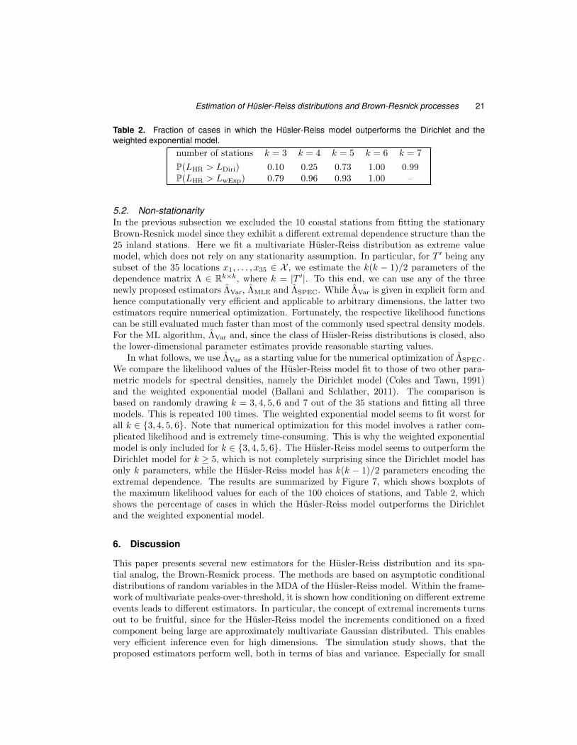
Estimation of Husler-Reiss distributions and Brown-Resnick processes 21
Table 2. Fraction of cases in which the Husler-Reiss model outperforms the Dirichlet and theweighted exponential model.
number of stations k = 3 k = 4 k = 5 k = 6 k = 7
P(LHR > LDiri) 0.10 0.25 0.73 1.00 0.99P(LHR > LwExp) 0.79 0.96 0.93 1.00 –
5.2. Non-stationarityIn the previous subsection we excluded the 10 coastal stations from fitting the stationaryBrown-Resnick model since they exhibit a different extremal dependence structure than the25 inland stations. Here we fit a multivariate Husler-Reiss distribution as extreme valuemodel, which does not rely on any stationarity assumption. In particular, for T ′ being anysubset of the 35 locations x1, . . . , x35 ∈ X , we estimate the k(k − 1)/2 parameters of thedependence matrix Λ ∈ Rk×k, where k = |T ′|. To this end, we can use any of the threenewly proposed estimators ΛVar, ΛMLE and ΛSPEC. While ΛVar is given in explicit form andhence computationally very efficient and applicable to arbitrary dimensions, the latter twoestimators require numerical optimization. Fortunately, the respective likelihood functionscan be still evaluated much faster than most of the commonly used spectral density models.For the ML algorithm, ΛVar and, since the class of Husler-Reiss distributions is closed, alsothe lower-dimensional parameter estimates provide reasonable starting values.
In what follows, we use ΛVar as a starting value for the numerical optimization of ΛSPEC.We compare the likelihood values of the Husler-Reiss model fit to those of two other para-metric models for spectral densities, namely the Dirichlet model (Coles and Tawn, 1991)and the weighted exponential model (Ballani and Schlather, 2011). The comparison isbased on randomly drawing k = 3, 4, 5, 6 and 7 out of the 35 stations and fitting all threemodels. This is repeated 100 times. The weighted exponential model seems to fit worst forall k ∈ {3, 4, 5, 6}. Note that numerical optimization for this model involves a rather com-plicated likelihood and is extremely time-consuming. This is why the weighted exponentialmodel is only included for k ∈ {3, 4, 5, 6}. The Husler-Reiss model seems to outperform theDirichlet model for k ≥ 5, which is not completely surprising since the Dirichlet model hasonly k parameters, while the Husler-Reiss model has k(k − 1)/2 parameters encoding theextremal dependence. The results are summarized by Figure 7, which shows boxplots ofthe maximum likelihood values for each of the 100 choices of stations, and Table 2, whichshows the percentage of cases in which the Husler-Reiss model outperforms the Dirichletand the weighted exponential model.
6. Discussion
This paper presents several new estimators for the Husler-Reiss distribution and its spa-tial analog, the Brown-Resnick process. The methods are based on asymptotic conditionaldistributions of random variables in the MDA of the Husler-Reiss model. Within the frame-work of multivariate peaks-over-threshold, it is shown how conditioning on different extremeevents leads to different estimators. In particular, the concept of extremal increments turnsout to be fruitful, since for the Husler-Reiss model the increments conditioned on a fixedcomponent being large are approximately multivariate Gaussian distributed. This enablesvery efficient inference even for high dimensions. The simulation study shows, that theproposed estimators perform well, both in terms of bias and variance. Especially for small
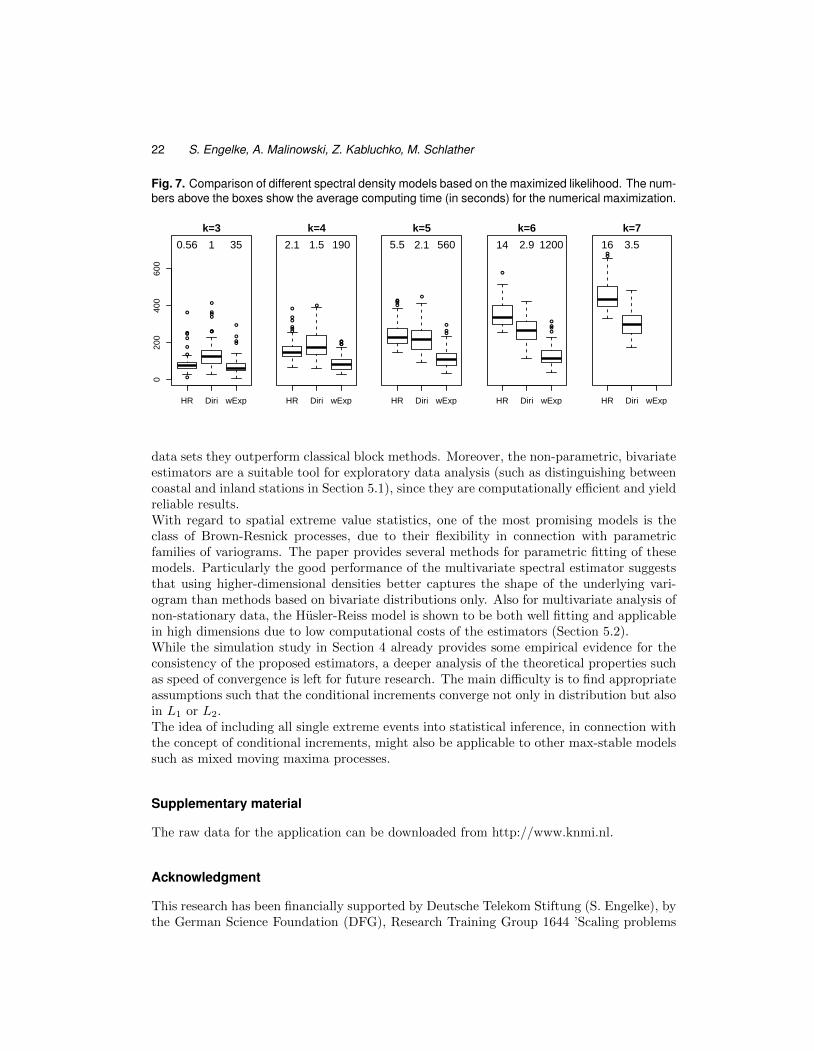
22 S. Engelke, A. Malinowski, Z. Kabluchko, M. Schlather
Fig. 7. Comparison of different spectral density models based on the maximized likelihood. The num-bers above the boxes show the average computing time (in seconds) for the numerical maximization.
●
●
●
●
●
●
●
●
●●
●
●
●
●
●
●
●
●
HR Diri wExp
020
040
060
0
k=3
0.56 1 35
●
●
●●
●
●
●
●●●●
HR Diri wExp
k=4
2.1 1.5 190
●
●●●
●
●●
●
HR Diri wExp
k=5
5.5 2.1 560
●
●
●
●
●
HR Diri wExp
k=6
14 2.9 1200●●
HR Diri wExp
k=7
16 3.5
data sets they outperform classical block methods. Moreover, the non-parametric, bivariateestimators are a suitable tool for exploratory data analysis (such as distinguishing betweencoastal and inland stations in Section 5.1), since they are computationally efficient and yieldreliable results.With regard to spatial extreme value statistics, one of the most promising models is theclass of Brown-Resnick processes, due to their flexibility in connection with parametricfamilies of variograms. The paper provides several methods for parametric fitting of thesemodels. Particularly the good performance of the multivariate spectral estimator suggeststhat using higher-dimensional densities better captures the shape of the underlying vari-ogram than methods based on bivariate distributions only. Also for multivariate analysis ofnon-stationary data, the Husler-Reiss model is shown to be both well fitting and applicablein high dimensions due to low computational costs of the estimators (Section 5.2).While the simulation study in Section 4 already provides some empirical evidence for theconsistency of the proposed estimators, a deeper analysis of the theoretical properties suchas speed of convergence is left for future research. The main difficulty is to find appropriateassumptions such that the conditional increments converge not only in distribution but alsoin L1 or L2.The idea of including all single extreme events into statistical inference, in connection withthe concept of conditional increments, might also be applicable to other max-stable modelssuch as mixed moving maxima processes.
Supplementary material
The raw data for the application can be downloaded from http://www.knmi.nl.
Acknowledgment
This research has been financially supported by Deutsche Telekom Stiftung (S. Engelke), bythe German Science Foundation (DFG), Research Training Group 1644 ’Scaling problems
Estimation of Husler-Reiss distributions and Brown-Resnick processes 23
in Statistics’ (A. Malinowski) and by Volkswagen Stiftung within the project ‘WEX-MOP’(M. Schlather).
Appendix
Proof (of Theorem 3.1). Note that
P{g(Xn) ∈ B
∣∣ Xn ∈ A− log u(n)}
= P{g(Xn + log u(n)) ∈ B
∣∣ Xn ∈ A− log u(n)}
=P{Xn ∈ (g−1(B)− log u(n)) ∩ (A− log u(n))
}P{Xn ∈ A− log u(n)
}=n/u(n)P
{X− log(n/u(n)) ∈ g−1(B) ∩A
}n/u(n)P {X− log(n/u(n)) ∈ A}
.
Thus, applying Prop. 5.17 in Resnick (2008), we obtain
limn→∞
P{g(Xn) ∈ B
∣∣ Xn ∈ A− log u(n)}
=µ(g−1(B) ∩A)
µ(A).
and the measure Qg,A is given by
Qg,A(B) =µ(g−1(B) ∩A)
µ(A), B ∈ B(S).
Proof (of Theorem 3.3). (a) The density of the exponent measure µ of the Husler-Reiss distribution (3) is given by
µ(dx0, . . . , dxk) =e−x0
(2π)k2 |detΣ|1/2
exp
(−1
2y>Σ−1y
)dx0 . . . dxk, x0, . . . , xk ∈ R,
where y = (x1 − x0 + 2λ21,0, . . . , xk − x0 + 2λ2
k,0)> and Σ = Ψk,(0,...,k)(Λ). For s =
(s1, . . . , sk) ∈ Rk, Bs = {y ∈ Rk : yi ≤ si, i = 1, . . . , k}, note that g−1(Bs) = {x ∈Rk+1 : xi − x0 ≤ si, i = 1, . . . , k}. Thus, for A1 = (0,∞)× Rk, we obtain
µ(g−1(Bs) ∩A1) =
∫ ∞0
e−x0
∫ x0+s1
−∞. . .
∫ x0+sk
−∞
exp(− 1
2y>Σ−1y
)(2π)
k2 |detΣ|1/2
dxk . . . dx0
= ΦM,Σ(s1, . . . , sk),
where ΦM,Σ is the cumulative distribution function of a k-variate normal distributionwith mean M = (−2λ2
1,0, . . . ,−2λ2k,0)> and covariance matrix Σ = Ψk,(0,...,k)(Λ).
Since µ(A1) = 1 and the family of sets {Bs, s ∈ Rk} is a generator of the Borelσ-algebra B(Rk) on Rk, the first assertion follows from the proof of Theorem 3.1.
(b) In the bivariate case the density of µ simplifies to
µ(dx, dy) =e−x
2λφ
(λ+
y − x2λ
)dx dy, x, y ∈ R,
24 S. Engelke, A. Malinowski, Z. Kabluchko, M. Schlather
with λ = λ0,1. We consider the set A2 = [−∞,0]C ⊂ R2 and note that µ(A2) = 2Φ(λ).It thus suffices to compute µ(g−1(Bt) ∩A2) for t ∈ R. For t < 0 we have
µ(g−1(Bt) ∩A2) =
∫ ∞0
∫ x+t
−∞
e−x
2λφ
(λ+
y − x2λ
)dy dx = Φ
(λ+
t
2λ
),
and similarly for t > 0,
µ(g−1(Bt) ∩A2) = µ(A2)− Φ
(λ− t
2λ
).
By the above considerations and the proof of Theorem 3.1 this yields
limn→∞
P{X(1) −X(0) ≤ t
∣∣∣X(0)n > log u(n) or X(1)
n > log u(n)}
=
{1
2Φ(λ)Φ(λ+ t
2λ
)for t < 0,
1− 12Φ(λ)Φ
(λ− t
2λ
)for t > 0.
In other words, X(1) −X(0) conditional on either X(0)n or X
(1)n being large converges
in distribution to some random variable Z with density
gλ(t) =1
4λΦ(λ)φ
(λ− |t|
2λ
), t ∈ R.
Proof (of Proposition 3.5). By Theorem 1 in Coles and Tawn (1991) we can com-pute the spectral density h as a derivative of the exponent measure ν(x) = − logGΛ(x),namely
∂ν(x)
∂x0 . . . ∂xk= −
(k∑i=0
xi
)−kh
(x0∑ki=0 xi
, . . . ,xk∑ki=0 xi
; Λ
).
Since all but one summands of the exponent measure ν vanish, it suffices to evaluate
∂
∂x0 . . . ∂xk(−1)k
∫log x0
∫log x1−z+2λ2
1,0
. . .
∫log xk−z+2λ2
k,0
φ (y|Σ) dy1 . . . dyk e−z dz, (28)
where φ ( · |Σ) is the density function of the k-dimensional normal distribution with covari-ance matrix Σ. Carrying out this computation yields (23).
References
Bacro, J.-N. and C. Gaetan (2012). Estimation of spatial max-stable models using thresholdexceedances. (Available from http://arxiv.org/abs/1205.1107).
Ballani, F. and M. Schlather (2011). A construction principle for multivariate extreme valuedistributions. Biometrika 98, 633–645.
Blanchet, J. and A. C. Davison (2011). Spatial modeling of extreme snow depth. Ann.Appl. Stat. 5, 1699–1725.
Estimation of Husler-Reiss distributions and Brown-Resnick processes 25
Boldi, M.-O. and A. C. Davison (2007). A mixture model for multivariate extremes. J. R.Stat. Soc. Ser. B Stat. Methodol. 69, 217–229.
Brown, B. M. and S. I. Resnick (1977). Extreme values of independent stochastic processes.J. Appl. Probab. 14, 732–739.
Coles, S. G. and J. A. Tawn (1991). Modelling extreme multivariate events. J. R. Stat.Soc. Ser. B Stat. Methodol. 53, 377–392.
Cooley, D., R. A. Davis, and P. Naveau (2010). The pairwise beta distribution: a flexibleparametric multivariate model for extremes. J. Multivariate Anal. 101, 2103–2117.
Cooley, D., P. Naveau, and P. Poncet (2006). Variograms for spatial max-stable randomfields. In P. Bertail, P. Soulier, and P. Doukhan (Eds.), Dependence in Probability andStatistics, Volume 187 of Lecture Notes in Statistics, Chapter 17, pp. 373–390. New York:Springer.
Davison, A. C. and M. M. Gholamrezaee (2012). Geostatistics of extremes. Proc. R. Soc.A 468, 581–608.
Davison, A. C., S. A. Padoan, and M. Ribatet (2012). Statistical modeling of spatialextremes. Statist. Sci. 27, 161–186.
Davison, A. C. and R. L. Smith (1990). Models for exceedances over high thresholds. J. R.Stat. Soc. Ser. B Stat. Methodol. 52, 393–442.
de Haan, L. and A. Ferreira (2006). Extreme value theory. Springer Series in OperationsResearch and Financial Engineering. New York: Springer.
de Haan, L. and T. T. Pereira (2006). Spatial extremes: models for the stationary case.Ann. Statist. 34, 146–168.
Dombry, C., F. Eyi-Minko, and M. Ribatet (2011). Conditional simulations of Brown-Resnick processes. (Available from http://arxiv.org/abs/1112.3891).
Engelke, S., A. Malinowski, M. Oesting, and M. Schlather (2012). Representa-tions of max-stable processes based on single extreme events. (Available fromhttp://arxiv.org/abs/1209.2303).
Genton, M. G., Y. Ma, and H. Sang (2011). On the likelihood function of Gaussian max-stable processes. Biometrika 98, 481–488.
Hashorva, E. (2006). On the multivariate Husler-Reiss distribution attracting the maximaof elliptical triangular arrays. Statist. Probab. Lett. 76, 2027–2035.
Hashorva, E., Z. Kabluchko, and A. Wubker (2012). Extremes of independent chi-squarerandom vectors. Extremes 15, 35–42.
Husler, J. and R.-D. Reiss (1989). Maxima of normal random vectors: between independenceand complete dependence. Statist. Probab. Lett. 7, 283–286.
Joe, H. (1990). Families of min-stable multivariate exponential and multivariate extremevalue distributions. Statist. Probab. Lett. 9, 75–81.
26 S. Engelke, A. Malinowski, Z. Kabluchko, M. Schlather
Kabluchko, Z. (2011). Extremes of independent Gaussian processes. Extremes 14, 285–310.
Kabluchko, Z., M. Schlather, and L. de Haan (2009). Stationary max-stable fields associatedto negative definite functions. Ann. Probab. 37, 2042–2065.
Kotz, S. and S. Nadarajah (2000). Extreme value distributions. London: Imperial CollegePress. Theory and applications.
Oesting, M., Z. Kabluchko, and M. Schlather (2012). Simulation of Brown-Resnick pro-cesses. Extremes 15, 89–107.
Padoan, S. A., M. Ribatet, and S. A. Sisson (2010). Likelihood-based inference for max-stable processes. J. Amer. Statist. Assoc. 105, 263–277.
Resnick, S. I. (2008). Extreme values, regular variation and point processes. Springer Seriesin Operations Research and Financial Engineering. New York: Springer.
Rootzen, H. and N. Tajvidi (2006). Multivariate generalized Pareto distributions.Bernoulli 12, 917–930.
Schlather, M. (2002). Models for stationary max-stable random fields. Extremes 5, 33–44.
Schlather, M. and J. A. Tawn (2003). A dependence measure for multivariate and spatialextreme values: Properties and inference. Biometrika 90, 139–156.
Smith, R. (1990). Max-stable processes and spatial extremes. Unpublished manuscript .
Tawn, J. A. (1990). Modelling multivariate extreme value distributions. Biometrika 77,245–253.