Estimation of Investment Model Cost Parameters for VSC

Estimation of Investment Model Cost Parametersfor VSC HVDC Transmission Infrastructure

Til Kristian Vranaa, Philipp Hartelb

aSINTEF Energi, Trondheim, NorwaybFraunhofer IWES, Kassel, Germany

Abstract

Investment model cost parameters for VSC HVDC transmission infrastructure continue to be associated with highuncertainty and their validity remains a crucial challenge. Thus, it is the key objective of this analysis to identify anew cost parameter set providing better investment cost estimates than currently available cost parameter sets. Thisparameter estimation is based on a previously conducted review of investment model cost parameters including itscollection of existing cost parameter sets and project cost reference data. By using a particle swarm optimisation,the overall error function of the review’s evaluation methodology is minimised to obtain an optimal parameter set.The results show, however, that the optimised parameter sets are far from being realistic and useful, which is why animproved overall error function is developed. Effectively penalising negative and near-zero cost parameter coefficients,this new overall error function delivers a realistic and well-performing cost parameter set when being minimised. In fact,the new parameter set produces better cost estimates for back-to-back, interconnector, and offshore wind connectionprojects than any of the existing cost parameter sets. Therefore, it is a valuable contribution and shall be considered infuture grid investment analyses involving VSC HVDC technology.

Keywords: Offshore grids, Transmission expansion planning, Cost model, HVDC, VSC, Parameter estimation,Particle swarm optimisation

1. Introduction

Voltage Source Converter (VSC) High Voltage DirectCurrent (HVDC) is the most suitable technology forfuture super grids and offshore grids in Europe [1] [2].While multiple investment analyses of future offshoregrid topologies have already been conducted (e.g. [3]),the subject of implementing integrated power gridscontinues to be an important research topic. As theoptimisation algorithms used for assessing investmentdecisions in offshore grid infrastructure rely on a costmodel and corresponding parameter sets, the validity ofthose parameter sets plays a crucial role.

However, it has been established in [4] that the costparameter sets which have been widely used by academiaand policymakers show significant variations from studyto study. They indicate a high level of uncertainty bothwhen comparing them against each other and whenevaluating them against reference cost data from realisedVSC HVDC projects. Acknowledging the fact thatthere are multiple and valid reasons for diverging costestimates obtained with those parameter sets, a new

parameter set based on the reference cost data for realisedprojects is needed to improve the validity of futuregrid investment and evaluation studies. Therefore, bydrawing on the collected parameter sets and referenceproject cost data in [4], a new parameter estimationapproach will be explored in this context to determinea new investment cost parameter set for VSC HVDCprojects which can be used in transmission expansionstudies.

In the remaining part of this article, Section 2summarises the cost model and parameter informationfor the following parameter estimation. Section 3introduces the particle swarm optimisation methodologywhich is used to compute the new parameter sets througherror minimisation. Two optimised cost parameter setsbased on the error function from [4] are presented inSection 4. Section 5 develops an extended overallerror function including the new realness category.In Section 6, the final cost parameter set obtainedfrom minimising the new overall error function ispresented. Section 7 discusses the obtained comparisonand evaluation results and Section 8 concludes the study.

Preprint submitted to Electric Power Systems Research 2018–02–19

This is the accepted version of an article published in Electric Power Systems Research DOI: 10.1016/j.epsr.2018.02.007

Nomenclature

AbbreviationsB2B Back-to-BackITC InterconnectorOWC Offshore Wind ConnectionPSO Particle Swarm OptimisationQEF Quadruple Error FunctionR RealnessTEF Triple Error FunctionGeneraldreale Ceiling of real (dreale = min {n ∈ N0 | n ≥ real})|set| Cardinality of setIndices and setsf ∈ Fi Set of branches within project ig ∈ Gi Set of nodes within project ih ∈ Hi Set of offshore nodes within project ii ∈ I j Set of projects within category jj ∈ J Set of project categories (J = {B2B, ITC,OWC})k ∈ K Set of cost parameter setsq ∈ Qk Set of cost parameters of parameter set kz ∈ Z Set of categories including realness (Z = J ∪ {R})Cost parameters and variablesBk

0 Fixed cost for building a branch with cost parameter setk (Me)

Bklp Length- and power-dependent cost for building a branch

with cost parameter set k (Me/GW·km)Bk

l Length-dependent cost for building a branch with costparameter set k (Me/km)

Ckest,i Estimated investment cost for project i (Me)

Cref,i Reference investment cost for project i (Me)Ccon

ref,i Reference contracted cost for project i (Me)

Nk0 Fixed cost for building a node with cost parameter set k

(Me)Nk

p Power-dependent cost for building a node with costparameter set k (Me/GW)

S k0 Fixed additional cost for building an offshore node with

cost parameter set k (Me)S k

p Power-dependent additional cost for building an offshorenode with cost parameter set k (Me/GW)

Technical parameters and variablesP j Maximum power rating for a single installation within

category j (GW). In case of a back-to-back system, thisis twice the system rating (two fully rated converters atone node).

lOHL, f Overhead line section length of branch f (km)lSMC, f Submarine cable section length of branch f (km)lUGC, f Underground cable section length of branch f (km)l f Total equivalent line length of branch f (km)p f Installed power rating of branch f (GW)pg/h Installed power rating at node g/h (GW). In case of a

back-to-back system, this is twice the system rating (twofully rated converters at one node).

Deviations and errorsεk

R Unscaled root-mean-square realness error for costparameter set k (-)

εkq,EXP Relative exponential deviation of parameter q for cost

parameter set k (-)εk

q,LOG Relative logarithmic realness deviation of parameter qfor cost parameter set k (-)

εkq,REL Relative realness deviation of parameter q for cost

parameter set k (-)A Constant scalar realness error scaling factor (-)Dk

i Project investment cost estimation deviation of project ifor cost parameter set k (-)

Dkj Category investment cost estimation deviation of category

j for cost parameter set k (-)Ek

QEF Overall root-mean-square error of four category errors(Quadruple Error Function) for cost parameter set k (-)

EkTEF Overall root-mean-square error of three category errors

(Triple Error Function) for cost parameter set k (-)Ek

R Root-mean-square realness error for cost parameter set k(-)

Ekq Realness error of cost parameter q for cost parameter set

k (-)Ek

j/z Category root-mean-square error of category j/z for costparameter set k (-)

2. Fundamentals

This section contains a summary of the most importantinformation, equations, and tables from [4], which areessential for the optimisation approach of this article. Inaddition, a new parameter set notation is introduced as itis convenient for all subsequent considerations.

2.1. Cost model

A linear uniform cost model has been defined in [4].It provides an approximation of the investment cost

associated with offshore grid HVDC infrastructureand yields a reasonable accuracy regarding long-termlarge-scale transmission expansion studies (e.g. [45]).The cost model is based on [46], [47] and [48].

Bear in mind that a mixed-integer linear cost modelyields significant benefits for long-term large-scaletransmission expansion planning problems and theoptimisation algorithms solving them, as computationtime and convergence face severe challenges when morecomplex cost models are applied.

2


Since the main equations explained in [4] areinevitable for the subsequent calculations, they arerepeated in this subsection. The linear uniform costmodel for VSC HVDC transmission investments isdefined by Equations (1) to (6):

Ckest,i =

Gi∑g

Nkg(pg) +

Fi∑f

Bkf (l f , p f ) +

Hi∑h

S kh(ph) (1)

Nkg(pg) = Nk

p · pg +

⌈pg

P j

⌉Nk

0 (2)

Bkf (l f , p f ) = Bk

lp · l f · p f +

⌈p f

P j

⌉ (Bk

l · l f + Bk0

)(3)

S kh(ph) = S k

p · ph +

⌈ph

P j

⌉S k

0 (4)

PB2B = 4 GW PITC = 2 GW POWC = 2 GW (5)

l f = lSMC, f +54

lUGC, f +23

lOHL, f (6)

It is important to stress that the installed power rating(pg, ph) corresponds to the total power rating of allconverters at a node, which is twice the system rating

for a back-to-back system (contains two fully-ratedconverters). This is the reason why PB2B is twice thesize of PITC and POWC.

In Equations (2) to (4), the ceiling operators areneeded to enforce the necessary integer investmentdecisions which have to be made as part of theoptimisation problem.

2.2. Parameter set notation

It is helpful to combine the seven parameters of acost parameter set in a mathematical set, as denoted inEquation (7):

Qk ={Bk

lp, Bkl , B

k0,N

kp,N

k0 , S

kp, S

k0

}∀k (7)

With that in mind, it is the primary goal of thisarticle to identify a new parameter set Qk constitutingan optimal fit for estimating investment costs of VSCHVDC infrastructure.

2.3. Reference project data

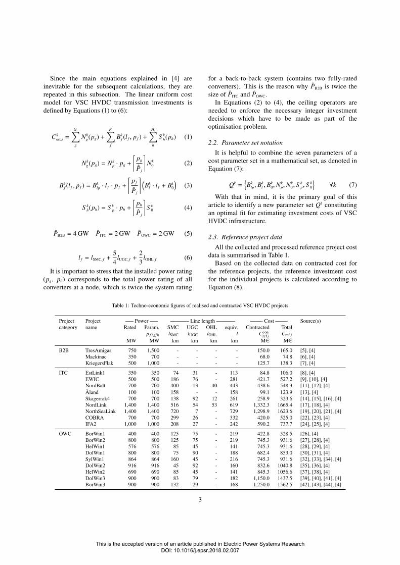
All the collected and processed reference project costdata is summarised in Table 1.

Based on the collected data on contracted cost forthe reference projects, the reference investment costfor the individual projects is calculated according toEquation (8).

Table 1: Techno-economic figures of realised and contracted VSC HVDC projects

Project Project —– Power —– ———– Line length ———– ——- Cost ——- Source(s)category name Rated Param. SMC UGC OHL equiv. Contracted Total

p f /g/h lSMC lUGC lOHL l Cconref,i Cref,i

MW MW km km km km Me Me

B2B TresAmigas 750 1,500 - - - - 150.0 165.0 [5], [4]Mackinac 350 700 - - - - 68.0 74.8 [6], [4]KriegersFlak 500 1,000 - - - - 125.7 138.3 [7], [4]

ITC EstLink1 350 350 74 31 - 113 84.8 106.0 [8], [4]EWIC 500 500 186 76 - 281 421.7 527.2 [9], [10], [4]NordBalt 700 700 400 13 40 443 438.6 548.3 [11], [12], [4]Åland 100 100 158 - - 158 99.1 123.9 [13], [4]Skagerrak4 700 700 138 92 12 261 258.9 323.6 [14], [15], [16], [4]NordLink 1,400 1,400 516 54 53 619 1,332.3 1665.4 [17], [18], [4]NorthSeaLink 1,400 1,400 720 7 - 729 1,298.9 1623.6 [19], [20], [21], [4]COBRA 700 700 299 26 - 332 420.0 525.0 [22], [23], [4]IFA2 1,000 1,000 208 27 - 242 590.2 737.7 [24], [25], [4]

OWC BorWin1 400 400 125 75 - 219 422.8 528.5 [26], [4]BorWin2 800 800 125 75 - 219 745.3 931.6 [27], [28], [4]HelWin1 576 576 85 45 - 141 745.3 931.6 [28], [29], [4]DolWin1 800 800 75 90 - 188 682.4 853.0 [30], [31], [4]SylWin1 864 864 160 45 - 216 745.3 931.6 [32], [33], [34], [4]DolWin2 916 916 45 92 - 160 832.6 1040.8 [35], [36], [4]HelWin2 690 690 85 45 - 141 845.3 1056.6 [37], [38], [4]DolWin3 900 900 83 79 - 182 1,150.0 1437.5 [39], [40], [41], [4]BorWin3 900 900 132 29 - 168 1,250.0 1562.5 [42], [43], [44], [4]

3


Cref,i =1110

Cconref,i ∀i ∈ IB2B

Cref,i =54

Cconref,i ∀i ∈ IITC (8)

Cref,i =54

Cconref,i ∀i ∈ IOWC

These estimated markups are accounting for thedifference between reference contractual cost Ccon

ref,i

and total project reference investment cost Cref,i.These differences are caused by many differentfactors, including, but not limited to, internal efforts,risk budget, engineering and concession costs, landpurchase, construction etc. The markup values arebased on [53], [34], [59] and unquotable personalcommunication with relevant industry stakeholders.

2.4. Cost parameter sets

The cost parameter sets considered in this article aregiven in Table 2. Compared to the cost parameter setsconsidered in [4], four parameter sets are neglected here.

The parameter sets Imperial College and Torbaghanare only meant for long distance transmission systems,and not for back-to-back systems. They do not containnodal cost parameters; all cost are proportional totransmission length. They do therefore not produceviable results for all of the three project categories, ascost for back-to-back stations (with zero transmissionlength) become zero. This has been shown in [4].Imperial College and Torbaghan have therefore not beenincluded in this study.

The parameter sets ENTSO-E and Madariaga containdata which lead to negative cost parameters when thegiven data is converted (extrapolated) to the here-usedformat of the linear uniform cost model. This indicates

that the data sets in question are not complete enough toallow for meaningful conversion to the linear uniformcost model. Negative cost parameters are unrealisticand lead to mathematical problems in the parameterestimation process. ENTSO-E and Madariaga havetherefore been disregarded in this study.

2.5. Average cost parameter set

Based on this reduced selection of cost parametersets, the average parameter set is calculated (displayedin Table 3). Naturally, it differs from the averageparameter set presented in [4] which also accounted forthe four parameter sets that are ignored here.

Table 3: Average cost parameter set

Parameter Unit QAVG

NAVGp

Me/GW 92.84NAVG

0 Me 34.90

BAVGlp

Me/GW·km 0.96BAVG

lMe/km 0.70

BAVG0 Me 5.00

S AVGp

Me/GW 116.26S AVG

0 Me 65.48

While six of the seven parameters are calculated asthe arithmetic mean, BAVG

0 is treated differently. Sinceonly one of the existing parameter sets actually considersBk

0 (WindSpeed), while the others have the parameter setto zero, calculating the mean would result in a very lowvalue, giving a poor representation of the associated cost.Instead of calculating the mean, it was therefore decidedto set BAVG

0 to the value provided by WindSpeed.

Table 2: Collected cost parameter sets

Name Year Nkp Nk

0 Bklp Bk

l Bk0 S k

p S k0 Source(s)

Me/GW Me Me/GW·km Me/km Me Me/GW Me

RealiseGrid 2011 83.00 0.00 2.58 0.07 0.00 0.00 28.00 [49], [4]WindSpeed 2011 216.00 6.50 0.67 0.36 5.00 23.00 17.30 [50], [4]Ergun et al. 2012 90.00 18.00 2.05 0.11 0.00 0.00 24.00 [51], [4]ETYS13 2013 60.80 63.17 0.29 1.06 0.00 216.60 143.66 [52], [4]NSTG 2013 58.90 54.90 1.23 0.00 0.00 130.83 0.00 [53], [54], [4]NSOG 2014 58.90 54.90 0.50 0,45 0.00 0.00 111.30 [55], [4]NorthSeaGrid 2015 65.00 54.00 0.35 1.85 0.00 125.00 218.95 [56], [4]OffshoreDC 2015 100.00 0.00 1.30 0.00 0.00 75.00 0.00 [57], [4]ETYS15 2015 103.00 62.60 0.63 1.45 0.00 475.90 46.07 [58], [4]

4


2.6. Project assessmentThe evaluation of a cost parameter set is carried out

by first calculating cost estimations for each individualreference project. These cost estimations are thencompared to the reference investment cost and therelative deviation is expressed on a logarithmic scale,as shown in Equation (9).

Dki = log2

(Ck

est,i

Cref,i

)∀i, k (9)

Relative deviations guarantee an adequate assessmentof both small and big projects. Using absolute costfigures would undervalue the correct estimation ofsmaller projects.

Logarithmic deviations account for the ratio betweenestimate and reality. It is important to use a logarithmicmeasure of the deviation to ensure a correct evaluationof both under- and overestimation.

Cost estimations range between the two worst possibleestimates {0,∞}, which are both equally evaluated on alogarithmic scale {−∞,+∞}. A non-logarithmic (linear)measure would inadequately evaluate them {−1,+∞},creating the wrong impression that zero cost would be amuch better estimate than infinite cost.

The non-logarithmic measure would equally evaluate{0, 2}, yielding {−1,+1}. {2} is by all means not a goodestimation, but it still represents a valid result. Onthe contrary, {0} implies that the infrastructure can bedeployed at zero cost, which is obviously wrong, leadingto over-investments in ’free’ assets when a transmissionexpansion planning optimisation is conducted. Thelogarithmic measure returns {−∞,+1} for this example,correctly reflecting the practical implications of the twoestimates.

As a consequence, the following evaluation ofparameter sets employs the relative logarithmic measure,as denoted in Equation (9).

2.7. Project category assessmentBased on the individual project deviations, the

category mean deviations are calculated according toEquation (10):

Dkj =

1|I j|

I j∑i

Dki ∀ j, k (10)

Based on the individual project deviations, thecategory root-mean-square errors are calculatedaccording to Equation (11):

Ekj =

√√1|I j|

I j∑i

(Dk

i

)2∀ j, k (11)

2.8. The TEF-based evaluation methodologyThe abbreviation ’TEF’ stands for the term Triple

Error Function because the overall error functionEquation (12) is based on the three project categories(B2B, ITC, OWC). This overall error function is identicalto Ek in [4], but since an improved error functionis introduced later in this article, a slightly amendednotation (Ek

TEF) is more convenient here.An overall assessment is achieved by calculating

the overall root-mean-square error of the categoryroot-mean-square errors, as expressed in Equation (12).

EkTEF =

√√√1|J|

J∑j

(Ek

j

)2∀k (12)

3. Optimisation methodology

In order to determine a new parameter set based onthe information summarised in Section 2, error functionshave to be optimised, i.e. minimised. However, theoverall error functions used here are non-linear anddifficult to minimise by using standard optimisationalgorithms. Instead, to minimise these functions, it isconvenient to employ a heuristic algorithm which is notmathematically guaranteed to find a solution but canoften be successfully applied to many problems. Forthe purpose of this study, a Particle Swarm Optimisation(PSO) is used as it can efficiently and reliably solveproblems [60] of this type.

PSO was first introduced by [61] as a concept for theoptimisation of non-linear functions using particle swarmmethodology. It is based on a population, referred to asa swarm, of particles simulating the social behaviourpatterns of organisms that live and interact within largegroups. In essence, these particles explore the searchspace to minimise the objective function, or landscape,of a problem. A detailed description of the underlyingprinciples, as well as a recent review of studies analysingand modifying PSO algorithms, can be found in [62].

Moreover, all PSO parameter estimation results werevalidated against a rather unsophisticated grid searchapproach. This computationally far more expensiveapproach yielded very similar solutions for the parameterestimation, hence confirming the validity of all resultsobtained from the PSO estimation.

4. The TEF-optimal cost parameter sets

The PSO algorithm is used to find the cost parameterset (seven variables) minimising the overall errorfunction given by Ek

TEF in Equation (12).

5


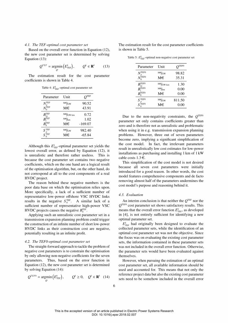
4.1. The TEF-optimal cost parameter setBased on the overall error function in Equation (12),

the new cost parameter set is determined by solvingEquation (13):

QT EF = argminQk

(Ek

TEF

), Qk ∈ Rk (13)

The estimation result for the cost parametercoefficients is shown in Table 4.

Table 4: EkTEF-optimal cost parameter set

Parameter Unit QTEF

NTEFp

Me/GW 90.52NTEF

0 Me 43.91

BTEFlp

Me/GW·km 0.72BTEF

lMe/km 1.02

BTEF0 Me -169.07

S TEFp

Me/GW 982.40S TEF

0 Me -65.84

Although this EkTEF-optimal parameter set yields the

lowest overall error, as defined by Equation (12), itis unrealistic and therefore rather useless. This isbecause the cost parameter set contains two negativecoefficients, which on the one hand are a logical resultof the optimisation algorithm, but, on the other hand, donot correspond at all to the cost components of a realHVDC project.

The reason behind these negative numbers is thepoor data base on which the optimisation relies upon.More specifically, a lack of a sufficient number ofrepresentative low-power offshore VSC HVDC linksresults in the negative S TEF

0 . A similar lack of asufficient number of representative high-power VSCHVDC projects causes the negative BTEF

0 .Applying such an unrealistic cost parameter set in a

transmission expansion planning problem could triggerthe construction of an infinite number of short low-powerHVDC links as their construction cost are negative,potentially resulting in an infinite profit.

4.2. The TEF0-optimal cost parameter setThe straight-forward approach to tackle the problem of

negative cost parameters is to constrain the optimisationby only allowing non-negative coefficients for the sevenparameters. Thus, based on the error function inEquation (12), the new cost parameter set is determinedby solving Equation (14):

QT EF0 = argminQk

(Ek

TEF

), Qk ≥ 0, Qk ∈ Rk (14)

The estimation result for the cost parameter coefficientsis shown in Table 5.

Table 5: EkTEF-optimal non-negative cost parameter set

Parameter Unit QTEF0

NTEF0p

Me/GW 98.82NTEF0

0 Me 35.31

BTEF0lp

Me/GW·km 1.30BTEF0

lMe/km 0.00

BTEF00 Me 0.00

S TEF0p

Me/GW 811.50S TEF0

0 Me 0.00

Due to the non-negativity constraints, the QTEF0

parameter set only contains coefficients greater thanzero and is therefore not as unrealistic and problematicwhen using it in e.g. transmission expansion planningproblems. However, three out of seven parametersbecome zero, implying a significant simplification ofthe cost model. In fact, the irrelevant parametersresult in unrealistically low cost estimates for low-powerinstallations as purchasing and installing 1 km of 1 kWcable costs 1.3e.

This simplification of the cost model is not desiredbecause all seven cost parameters were initiallyintroduced for a good reason. In other words, the costmodel features comprehensive components and de factoremoving almost half of the parameters undermines thecost model’s purpose and reasoning behind it.

4.3. Evaluation

An interim conclusion is that neither the QTEF nor theQTEF0 cost parameter set shows satisfactory results. Thismeans that the overall error function Ek

TEF, as developedin [4], is not entirely sufficient for identifying a newoptimal parameter set.

EkTEF had originally been designed to evaluate the

collected parameter sets, while the identification of anoptimal cost parameter set was not the objective. Sincethe focus was on evaluating the existing cost parametersets, the information contained in these parameter setswas not included in the overall error function. Otherwise,the parameter sets would have been evaluated againstthemselves.

However, when pursuing the estimation of an optimalcost parameter set, all available information should beused and accounted for. This means that not only thereference project data but also the existing cost parametersets need to be somehow included in the overall error

6


function. It is therefore sensible to develop an extendedoverall error function by incorporating the informationof existing cost parameter sets.

5. The QEF-based evaluation methodology

’QEF’ abbreviates the term Quadruple Error Functionbecause the improved overall error function inEquation (24) is based on four components: the threeproject categories and the new ’realness’ category.Essentially, the realness measure is based on thedeviations from the QAVG cost parameter set. Theextended overall error function is called Ek

QEF and ithas to be distinguished from Ek

TEF, which is identicalto Ek in [4]. Hence, the new Ek

QEF takes into accountall the information gathered from reference projects andexisting cost parameter sets.

It is important that the improved error function EkQEF is

backward compatible and does not distort the results ofthe error function Ek

TEF because it should still be usefulfor assessing existing parameter sets. Otherwise, Ek

QEF

could not replace the existing error function EkTEF.

5.1. Definition of realness

As discussed in Subsection 4.1 and Subsection 4.2,both Ek

TEF-optimal parameter sets gave unsatisfactoryresults because the resulting coefficients are not realistic.In order to implement the improved error function, thissubjective assessment of realness must be expressed inmathematical terms so that the optimisation algorithmcan factor it in. As mentioned before, it was decidedto base the realness measure on the deviations from theQAVG cost parameter set.

A natural first approach is using a relativelogarithmic deviation, similar to Equation (9), resultingin Equation (15):

εkq,LOG = log2

(qk

qAVG

)∀q ∈ Qk, ∀k (15)

However, this approach turns out to be not feasible.A parameter set of which at least one parameter isdisappearing, i.e. equal to zero, would produce adeviation of minus infinity. This implies that allparameter sets except WindSpeed would be assessed withan infinite error. Therefore, such a deviation functionis not particularly useful for assessing the existing costparameter sets.

Another trivial approach is to rely on relativedeviation without logarithmic consideration, resultingin Equation (16):

εkq,REL =

qk − qAVG

qAVG∀q ∈ Qk, ∀k (16)

This deviation definition solves the issue of thedisappearing parameters because they are assessed witha deviation of one instead of infinity. Despite that, it doesnot adequately penalise negative coefficients, and, as aconsequence, still permits the optimal parameter set tocontain negative parameters.

To capture the intended realness of parametercoefficients, the corresponding mathematical term needsto:

• return a finite number if zero is the input

• have a highly negative slope (first derivative) forinputs close to zero

• have an almost flat slope for inputs around theaverage parameter value

In this context, an inverse exponential function waschosen as the most suitable mathematical function tofulfil the expressed requirements.

Based on Equation (7), the unscaled realness deviationfor a single parameter k of a parameter set q can beexpressed by Equation (17):

εkq,EXP = exp−

(qk

1/4 qAVG

)∀q ∈ Qk, ∀k (17)

Here, the factor 1/4 is important since it determines theshape of the exponential function.

Basically, a small factor results in a steep slope atzero and a gentle slope around the average parameter.Conversely, a larger factor reduces the function’s slopeat zero but widens the steep slope area around zero. Thisimplies a systematic overestimation of the investmentcost because a larger factor favours high parameters. Ithas to be stated that there is no scientific means to setthis factor to a correct value. The factor 1/4, which wasfinally selected and applied, has been determined by trialand error yielding the best compromise to deliver anadequate error function.

5.2. Improved error function including realness

Based on the unscaled realness deviation for a singleparameter in Equation (17), the unscaled root-mean

7


square realness error of a parameter set k can be definedby Equation (18):

εkR =

√√√1|Qk |

Qk∑q

(εk

q,EXP

)2∀k (18)

The unscaled function in Equation (17) returns εkq,EXP =

1 for a disappearing parameter (qk = 0). This amplitudeis arbitrary and does not relate to the other error functionswhich are based on the project categories. To betteralign the realness error amplitude with the other errorcategories, the ratio between unscaled realness error andthe Ek

TEF-based overall error is calculated as the mean forall existing cost parameter sets presented in Table 2, seeEquation (19):

A =

1|K|

∑Kk Ek

TEF

1|K|

∑Kk ε

kR

(19)

A is a constant scalar and can be used to scale therealness error, so that its amplitude relates to the othererror amplitudes, as shown in Equation (20):

Ekq = Aεk

q,EXP ∀q ∈ Qk, ∀k (20)

The scaling factor also applies to the realness error fora parameter set from Equation (18), which is denoted asEquation (21):

EkR = Aεk

R =

√√√1|Qk |

Qk∑q

(Ek

q

)2∀k (21)

Incorporating the scaled realness error fromEquation (21) into the overall error functionEquation (12) as a fourth category results in theimproved Quadruple Error Function:

EkQEF =

√√√1

1 + |J|

(EkR

)2+

J∑j

(Ek

j

)2

∀k (22)

Formally, the realness error can be added as a furthercategory which is denoted in Equation (23):

Z = J ∪ {R} (23)

By using the combined category set Z fromEquation (23), Equation (22) can be simplified toEquation (24):

EkQEF =

√√1|Z|

Z∑z

(Ek

z

)2∀k (24)

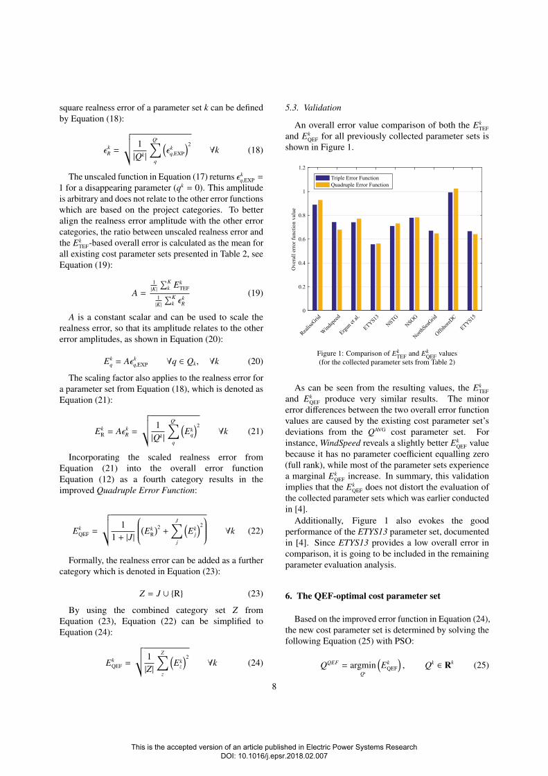
5.3. Validation

An overall error value comparison of both the EkTEF

and EkQEF for all previously collected parameter sets is

shown in Figure 1.

Realise

Grid

Wind

speed

Ergun e

t al.

ETYS13NSTG

NSOG

NorthS

eaGrid

Offsho

reDC

ETYS150

0.2

0.4

0.6

0.8

1

1.2

Ove

rall

erro

r fun

ctio

n va

lue

Triple Error FunctionQuadruple Error Function

Figure 1: Comparison of EkTEF and Ek

QEF values(for the collected parameter sets from Table 2)

As can be seen from the resulting values, the EkTEF

and EkQEF produce very similar results. The minor

error differences between the two overall error functionvalues are caused by the existing cost parameter set’sdeviations from the QAVG cost parameter set. Forinstance, WindSpeed reveals a slightly better Ek

QEF valuebecause it has no parameter coefficient equalling zero(full rank), while most of the parameter sets experiencea marginal Ek

QEF increase. In summary, this validationimplies that the Ek

QEF does not distort the evaluation ofthe collected parameter sets which was earlier conductedin [4].

Additionally, Figure 1 also evokes the goodperformance of the ETYS13 parameter set, documentedin [4]. Since ETYS13 provides a low overall error incomparison, it is going to be included in the remainingparameter evaluation analysis.

6. The QEF-optimal cost parameter set

Based on the improved error function in Equation (24),the new cost parameter set is determined by solving thefollowing Equation (25) with PSO:

QQEF = argminQk

(Ek

QEF

), Qk ∈ Rk (25)

8


Table 6: EkQEF-optimal cost parameter set

Parameter Unit Value

NQEFp

Me/GW 112.99NQEF

0 Me 23.50

BQEFlp

Me/GW·km 0.98BQEF

lMe/km 0.27

BQEF0 Me 3.63

S QEFp

Me/GW 723.42S QEF

0 Me 57.32

Table 6 shows the estimation result for the costparameter coefficients.

The new realness error category ensures non-negativecoefficients for all seven cost parameters of Qk,particularly Bk

0, Bkl , and S k

0. As opposed to both QTEF

and QTEF0, the QQEF cost parameter set uses all availableparameters of the VSC HVDC cost model in a realisticmanner.

7. Evaluation of the cost parameter sets

To evaluate the new QQEF parameter set, an assessmentand comparison of its parameter coefficients, resultingdeviations, and overall errors against the other parametersets is presented in this section.

7.1. Comparison of cost parameter coefficients

The cost parameters Nkp and Nk

0 are presented inFigure 2, constituting the node cost part of the investmentmodel in Equation (2).

0

50

100

150

N p in

M€/

GW

ETYS13 QAVG QTEF QTEF0 QQEF0

20

40

60

80

N 0 in

M€

kk

Figure 2: Comparison of node cost parameters Nkp and Nk

0

While the mathematical, but unrealistic node costparameter optimum is represented by QTEF, with QTEF0

and QAVG lying quite close to it, the QQEF parameter setshows the highest Nk

p and lowest N0 values.The cost parameters Bk

lp, Bkl and Bk

0 are presentedin Figure 3, representing the branch cost part of theinvestment model in Equation (3).

0

0.5

1

1.5

B lp

in M

€/G

W/k

m

0

0.5

1

1.5

B l in

M€/

km

ETYS13 QAVG QTEF QTEF0 QQEF-10

-5

0

5

10B 0

in M

€

-169.1

kk

k

Figure 3: Comparison of branch cost parameters Bklp, Bk

l and Bk0

From the figure, it becomes obvious that the realnesscategory came into effect, particularly for Bk

l andBk

0. With QAVG and QQEF being the only two costparameter sets with reasonable, i.e. non-disappearingand non-negative, coefficients, the branch parameters ofthe QQEF cost parameter set lie between the QTEF0 andthe QAVG set. This effect was exactly intended by therealness component in the new overall error function.

The cost parameters S kp and S k

0 are presented inFigure 4, contributing the additional offshore costpart (deployment at sea) of the investment model inEquation (4).

0

500

1000

S p in

M€/

GW


0

100

200

S 0 in

M€

kk

Figure 4: Comparison of offshore cost parameters S kp and S k

0

9


Importantly, all optimised sets show significantlyhigher offshore cost parameters, which is a logicalconsequence of the substantial investment costunderestimations of offshore wind connection projectsreported in [4]. Similar to the branch cost parameters,the S k

p and S k0 parameters of QQEF result in a trade-off

between the QTEF0 and QAVG cost parameter set.

7.2. Assessment of deviations

The project deviations and category deviation ofinvestment costs for back-to-back projects are illustratedin Figure 5.


-1.5

-1

-0.5

0

0.5

1

1.5

2

Proj

ect a

nd c

ateg

ory

inve

stm

ent c

ost d

evia

tions

-0.054 -0.098 -0.002 -0.032 -0.049

TresAmigasMackinacKriegersFlakBack-to-back

Figure 5: Deviations Dki for back-to-back projects

(category deviation DkB2B shown in boxes)

In comparison, the results indicate only minordeviations among all considered parameter sets. Asexpected, the QTEF cost parameter set yields the smallestcategory deviation. That said, back-to-back projectcategory deviations of QQEF are only slightly higher, butstill very small.

The project deviations and category deviationof investment costs for interconnector projects areillustrated in Figure 6.

As can be seen from the resulting interconnectorcategory deviations, all optimised parameter sets,i.e. QTEF, QTEF0, and QQEF, avoid the systematicoverestimations becoming obvious for ETYS13 andQAVG.

Figure 7 illustrates the project deviations andcategory deviation of investment costs for offshore windconnection projects.


-1.5

-1

-0.5

0

0.5

1

1.5

2

Proj

ect a

nd c

ateg

ory

inve

stm

ent c

ost d

evia

tions

0.364 0.407 -0.010 0.026 0.062

EstLink1EWICNordBaltSkagerrak4Åland

NordLinkNorthSeaLinkCOBRAIFA2Interconnector

Figure 6: Deviations Dki for interconnector projects

(category deviation DkITC shown in boxes)


-1.5

-1

-0.5

0

0.5

1

1.5

2

Proj

ect a

nd c

ateg

ory

inve

stm

ent c

ost d

evia

tions

-0.385 -0.667 0.011 0.006 0.008

Borwin1Borwin2Helwin1Dolwin1Sylwin1Dolwin2Helwin2Dolwin3Borwin3Offshore wind connection

Figure 7: Deviations Dki for offshore wind connector projects

(category deviation DkOWC shown in boxes)

By contrast to the interconnector deviations, the costsof offshore wind connection projects are systematicallyunderestimated by ETYS13 and QAVG, which is no longerthe case for the Ek

TEF-optimal and EkQEF-optimal cost

parameter sets.Clearly, single projects are still over- or

underestimated, but, when comparing them against theexisting cost parameter sets and QAVG, the three projectcategory deviations are significantly better for the threeoptimised cost parameter sets, i.e. QTEF, QTEF0, andQQEF.

10


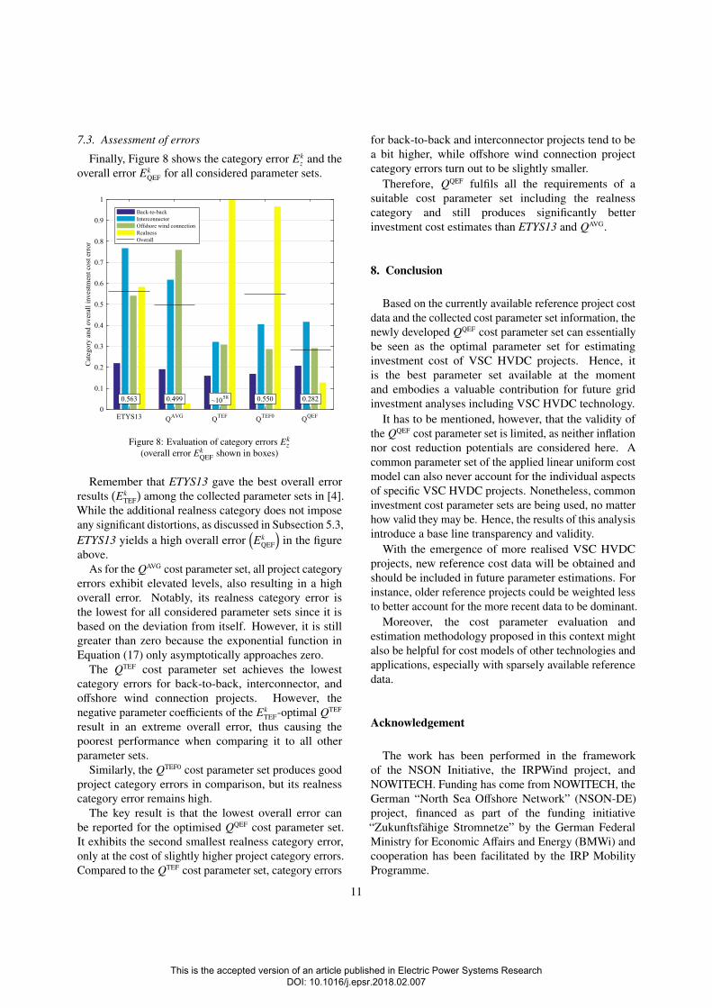
7.3. Assessment of errors

Finally, Figure 8 shows the category error Ekz and the

overall error EkQEF for all considered parameter sets.

ETYS13 QAVG QTEF QTEF0 QQEF0

0.1

0.2

0.3

0.4

0.5

0.6

0.7

0.8

0.9

1

Cat

egor

y an

d ov

eral

l inv

estm

ent c

ost e

rror

0.563 0.499 ~1058 0.550 0.282

Back-to-backInterconnectorOffshore wind connectionRealnessOverall

Figure 8: Evaluation of category errors Ekz

(overall error EkQEF shown in boxes)

Remember that ETYS13 gave the best overall errorresults

(Ek

TEF

)among the collected parameter sets in [4].

While the additional realness category does not imposeany significant distortions, as discussed in Subsection 5.3,ETYS13 yields a high overall error

(Ek

QEF

)in the figure

above.As for the QAVG cost parameter set, all project category

errors exhibit elevated levels, also resulting in a highoverall error. Notably, its realness category error isthe lowest for all considered parameter sets since it isbased on the deviation from itself. However, it is stillgreater than zero because the exponential function inEquation (17) only asymptotically approaches zero.

The QTEF cost parameter set achieves the lowestcategory errors for back-to-back, interconnector, andoffshore wind connection projects. However, thenegative parameter coefficients of the Ek

TEF-optimal QTEF

result in an extreme overall error, thus causing thepoorest performance when comparing it to all otherparameter sets.

Similarly, the QTEF0 cost parameter set produces goodproject category errors in comparison, but its realnesscategory error remains high.

The key result is that the lowest overall error canbe reported for the optimised QQEF cost parameter set.It exhibits the second smallest realness category error,only at the cost of slightly higher project category errors.Compared to the QTEF cost parameter set, category errors

for back-to-back and interconnector projects tend to bea bit higher, while offshore wind connection projectcategory errors turn out to be slightly smaller.

Therefore, QQEF fulfils all the requirements of asuitable cost parameter set including the realnesscategory and still produces significantly betterinvestment cost estimates than ETYS13 and QAVG.

8. Conclusion

Based on the currently available reference project costdata and the collected cost parameter set information, thenewly developed QQEF cost parameter set can essentiallybe seen as the optimal parameter set for estimatinginvestment cost of VSC HVDC projects. Hence, itis the best parameter set available at the momentand embodies a valuable contribution for future gridinvestment analyses including VSC HVDC technology.

It has to be mentioned, however, that the validity ofthe QQEF cost parameter set is limited, as neither inflationnor cost reduction potentials are considered here. Acommon parameter set of the applied linear uniform costmodel can also never account for the individual aspectsof specific VSC HVDC projects. Nonetheless, commoninvestment cost parameter sets are being used, no matterhow valid they may be. Hence, the results of this analysisintroduce a base line transparency and validity.

With the emergence of more realised VSC HVDCprojects, new reference cost data will be obtained andshould be included in future parameter estimations. Forinstance, older reference projects could be weighted lessto better account for the more recent data to be dominant.

Moreover, the cost parameter evaluation andestimation methodology proposed in this context mightalso be helpful for cost models of other technologies andapplications, especially with sparsely available referencedata.

Acknowledgement

The work has been performed in the frameworkof the NSON Initiative, the IRPWind project, andNOWITECH. Funding has come from NOWITECH, theGerman “North Sea Offshore Network” (NSON-DE)project, financed as part of the funding initiative“Zukunftsfahige Stromnetze” by the German FederalMinistry for Economic Affairs and Energy (BMWi) andcooperation has been facilitated by the IRP MobilityProgramme.

11


References

[1] T. K. Vrana, System Design and Balancing Control of the NorthSea Super Grid, Doctoral Thesis, NTNU- Norwegian Universityof Science and Technology, Trondheim, Norway (2013).

[2] T. K. Vrana, R. E. Torres-Olguin, Report: Technologyperspectives of the North Sea Offshore and storage Network(NSON), 2015.

[3] J. de Decker, P. Kreutzkamp, P. Joseph, A. Woyte, S. Cowdroy,P. McGarley, L. Warland, H. G. Svendsen, J. Volker, C. Funk,H. Peinl, J. Tambke, L. von Bremen, K. Michalowska, G. Caralis,Offshore Electricity Grid Infrastructure in Europe, OffshoreGrid- Final Report (2011).

[4] P. Hartel, T. K. Vrana, T. Hennig, M. von Bonin,E. J. Wiggelinkhuizen, F. D. Nieuwenhout, Review ofinvestment model cost parameters for VSC HVDC transmissioninfrastructure, Electric Power Systems Research 151 (2017)419–431.

[5] Alstom Grid Press Releases, Alstom Grid will provide TresAmigas LLC in the USA with first-of-its-kind Smart GridSuperStation, 21.04.2011.

[6] ABB Press Releases, ABB wins $90 million power order toimprove grid stability in Michigan: HVDC Light system tofacilitate power flow control and integration of renewables,23.02.2012.

[7] ABB Press Releases, ABB wins $140 million order to boostintegration of renewables in Europe: HVDC converter stationto link Danish and German power grids and enhance energysecurity, 10.03.2016.

[8] ABB Press Releases, ABB wins bid for underground power linkbetween Estonia and Finland: Unique HVDC Light technologyhelps to expand Trans-European Network, 04.02.2005.

[9] ABB Press Releases, ABB wins power transmission order worth$550 million from irish grid operator: Ireland-u.k. power link tostrengthen grid reliability and security of supply, 29.03.2009.

[10] L. Brand, R. de Silva, E. Bebbington, K. Chilukuri, Grid WestProject: HVDC Technology Review, 2014.

[11] ABB Press Releases, ABB wins $580-million powertransmission order in Europe: New transmission link strengthensintegration of Baltic energy markets with northern Europe,20.12.2010.

[12] Reuters, UPDATE 1-ABB wins $580 mln Nordic-Baltic powerorder, 20.12.2010.

[13] ABB Press Releases, ABB wins $130-million HVDC orderfor subsea power transmission link in Finland: HVDC lighttechnology secures power supply and grid reliability to Finnisharchipelago, 13.12.2012.

[14] ABB Press Releases, ABB wins $180 million order forNorway-Denmark power transmission link, 10.02.2011.

[15] N. P. Releases, Nexans wins 87 million Euro contract forSkagerrak 4 subsea HVDC power cable between Denmark andNorway, 07.01.2011.

[16] Prysmian Group Press Releases, Official inauguration of theSkagerrak 4 electrical interconnection between Norway andDenmark, 12.03.2015.

[17] ABB Press Releases, ABB wins $900 million order to connectNorwegian and German power grids: NordLink project will beEurope’s longest HVDC power grid interconnection and enablethe transmission of 1,400 megawatts (MW) of renewable energy,19.03.2015.

[18] Nexans, NordLink HVDC interconnector between Norway andGermany will use Nexans’ subsea power cables, 12.02.2015.

[19] ABB Press Releases, ABB wins $450 million order forNorway-UK HVDC interconnection, 14.07.2015.

[20] Prysmian Group Press Releases, Prysmian, new contract worth

arounde 550 M for an HVDC submarine interconnector betweenNorway and the UK, 14.07.2015.

[21] Nexans Press Releases, NSN Link will interconnect Nordic andBritish energy markets with the world’s longest subsea powerlink incorporating Nexans’ HVDC cable technology, 14.07.2015.

[22] Siemens AG Press Releases, Siemens wins order for HVDC linkbetween Denmark and Holland, 01.02.2016.

[23] Prysmian Group Press Releases, Prysmian secures contract wortharound e250 M for a submarine power cable link between theNetherlands and Denmark, 01.02.2016.

[24] ABB Press Releases, ABB selected for a e270 million order forUK-France power link: ABB is awarded the HVDC converterstations for the IFA2 interconnection, 07.04.2017.

[25] Prysmian Group Press Releases, The project worth arounde350M has been awarded to Prysmian by a joint venture betweenfrench RTE and UK National Grid IFA2 LTD, 07.04.2017.

[26] ABB Press Releases, ABB wins power order worth morethan $400 million for world’s largest offshore wind farm:Innovative technology will connect wind-generated electricpower to grid, 18.09.2007.

[27] Siemens AG Press Releases, Siemens receives order fromtranspower to connect offshore wind farms via HVDC link: Orderworth more than EUR500 million for the consortium, 11.06.2010.

[28] Prysmian Group Press Releases, Prysmian secures a further majorproject worth more than e150 M from German Transpower forthe HelWin1 grid connection of offshore wind farms, 16.07.2010.

[29] Siemens AG Press Releases, Siemens erhalt vontranspower weiteren Auftrag zur Anbindung vonOffshore-Windenergieanlagen: Auftragswert fur Konsortiumliegt bei rund einer halben Milliarde Euro, 16.07.2010.

[30] ABB Press Releases, ABB wins order for offshore windpower connection worth around $ 700 million: HVDC Lighttransmission link will connect three North Sea wind farms toGerman power grid, 16.07.2010.

[31] A. Abdalrahman, E. Isabegovic, DolWin1 - challenges ofconnecting offshore wind farms, in: 2016 IEEE InternationalEnergy Conference (ENERGYCON), pp. 1–10.

[32] Siemens AG Press Releases, Green power from the North Sea:Siemens to install grid link for DanTysk offshore wind farm,26.01.2011.

[33] Prysmian Group Press Releases, Prysmian secures SylWin1project by TenneT for the cable connection of offshore windfarms in the North Sea to the German power grid, 26.01.2011.

[34] G. Fichtner, Beschleunigungs- und Kosten senkungspotenzialebei HGU-Offshore-Netzanbindungsprojekten - Langfassung,2016.

[35] ABB Press Releases, ABB wins $1 billion order for offshore windpower connection: HVDC Light transmission link will connectNorth Sea wind farms to German power grid, 02.08.2011.

[36] M. Sprenger, Kontrakt til 1,7 milliarder, Teknisk Ukeblad(04.08.2011).

[37] Siemens AG Press Releases, Siemens brings HelWin clusterwindfarm on line: Offshore HVDC platform for low-losstransmission to the onshore grid, 02.08.2011.

[38] Prysmian Group Press Releases, Prysmian secures HelWin2project worth in excess of e 200 M for the grid connectionof Offshore Wind Farms in Germany, 01.08.2011.

[39] Handelsblatt, Offshore-Plattform: Neuer Großauftrag fur NordicYards, Handelsblatt (26.02.2013).

[40] Prysmian Group Press Releases, Prysmian secures DolWin3project worth in excess of e 350 M for the grid connection ofoffshore wind farms in Germany, 26.02.2013.

[41] Alstom Press Releases, Offshore-Windenergie: Vergabe vonDolWin3 bringt Energiewende voran, 26.02.2013.

[42] Siemens AG Press Releases, Siemens receives major order for

12


BorWin3 North Sea grid connection from TenneT, 15.04.2014.[43] Siemens AG, Hauptversammlung der Siemens AG: Rede Joe

Kaeser, 2015.[44] Prysmian Group Press Releases, Prysmian Secures BorWin3

Project Worth In Excess Of e 250 M, 15.04.2014.[45] G. Sanchis, P. van Hove, T. Jerzyniak, B. Bakken, T. Anderski,

E. Peirano, R. Pestana, B. de Clercq, G. Migliavacca, M. Czernie,P. Panciatici, M. Paun, N. Grisey, B. Betraoui, D. Lasserre,C. Pache, E. Momot, A.-C. Leger, C. Counan, C. Poumarede,M. Papon, J. Maeght, B. Seguinot, S. Agapoff, M.-S. Debry,D. Huertas-Hernando, L. Warland, T. K. Vrana, H. Farahmand,T. Butschen, Y. Surmann, C. Strotmann, S. Galant, A. Vafeas,N. Machado, A. Pitarma, R. Pereira, J. Madeira, J. Moreira,M. R. Silva, D. Couckuyt, P. van Roy, F. Georges, C. R. Prada,V. Gombert, R. Stornowski, C. Paris, N. Bragard, J. Warichet,A. Labatte, F. Careri, S. Rossi, A. Zani, D. Orlic, D. Vlaisavljevic,H. Seidl, J. Volker, N. Grimm, J. Balanowski, M. Marcolt, S.-L.Soare, T. Linhart, K. Maslo, M. Emery, C. Dunand, P. C. Lopez,M. Haller, L. Drossler, T. Nippert, B. Guzzi, S. Ibba, S. Moroni,C. Gadaleta, P. di Cicco, E. M. Carlini, A. Ferrante, C. Vergine,G. Taylor, M. Golshani, A. H. Alikhanzadeh, Y. Bhavanam,L. Olmos, A. Ramos, M. Rivier, L. Sigris, S. Lumbreras,F. Banez-Chicharro, L. Rouco, F. Echavarren, M. R. Partidario,R. Soares, M. Monteiro, N. Oliveira, D. van Hertem, K. Bruninx,D. Huang, E. Delarue, H. Ergun, K. de Vos, D. Villacci, K. Strunz,M. Gronau, A. Weber, C. Casimir, L. Lorenz, A. Dusch, J. Sijm,F. Nieuwenhout, A. van der Welle, Ozge Ozdemir, M. Bajor,M. Wilk, R. Jankowski, B. Sobczak, A. Caramizaru, G. Lorenz,F. Bauer, C. Weise, V. Wendt, E. Zaccone, E. Giovannetti,I. Pineda, O. Blank, M. Margarone, J. Roos, P. Lundberg,B. Westman, G. Keane, B. Hickman, J. Gaventa, M. Dufour,M. Juszczuk, M. Małecki, P. Ziołek, R. Eales, C. Twigger-Ross,W. Sheate, P. Phillips, S. Forrest, K. Brooks, R. M. Sørensen,N. T. Franck, S. Osterbauer, K. Elkington, J. Setreus, J. L.Fernandez-Gonzalez, O. Brenneisen, I. Kabouris, Europe’s futuresecure and sustainable electricity infrastructure - e-Highway2050project results, e-Highway2050 Project Booklet (2015).

[46] H. G. Svendsen, Planning Tool for Clustering and OptimisedGrid Connection of Offshore Wind Farms, Energy Procedia 35(2013) 297–306.

[47] T. Trotscher, M. Korpås, A framework to determine optimaloffshore grid structures for wind power integration and powerexchange, Wind Energy 14 (2011) 977–992.

[48] T. K. Vrana, Review of HVDC Component Ratings: XLPECables and VSC Converters, IEEE EnergyCon, Leuven (2016).

[49] A. L’Abbate, G. Migliavacca, Review of costs of transmissioninfrastructures, including cross border connections: REseArch,methodoLogIes and technologieS for the effective developmentof pan-European key GRID infrastructures to support theachievement of a reliable, competitive and sustainable electricitysupply (REALISEGRID): Deliverable d3.3.2, 2011.

[50] J. Jacquemin, D. Butterworth, C. Garret, N. Baldock,A. Henderson, Windspeed D2.2: Inventory of location specificwind energy cost, 2011.

[51] H. Ergun, D. van Hertem, R. Belmans, TransmissionSystem Topology Optimization for Large-Scale Offshore WindIntegration, IEEE Transactions on Sustainable Energy 3 (2012)908–917.

[52] P. Sheppard, Electricity Ten Year Statement - Appendix E, 2013.[53] F. D. J. Nieuwenhout, M. van Hout, Cost, benefits, regulations

and policy aspects of a North Sea Transnational Grid, 2013.[54] J. T. G. Pierik, North Sea Transnational Grid: Evaluation of

NSTG options (WP2), 2014.[55] S. Cole, P. Martinot, S. Rapoport, G. Papaefthymiou, V. Gori,

Study of the benefits of a meshed offshore grid in Northern Seas

region: Final Report, 2014.[56] A. Flament, P. Joseph, G. Gerdes, L. Rehfeldt, A. Behrens,

A. Dimitrova, F. Genoese, I. Gajic, M. Jafar, N. Tidemand,Y. Yang, J. Jansen, F. Nieuwenhout, K. Veum, I. Konstantelos,D. Pudjianto, G. Strbac, NorthSeaGrid Final Report, 2015.

[57] N. Helisto, V. C. Tai, OffshoreDC: Electricity market and powerflow impact of wind power and DC grids in the Baltic Sea:Research Report, 2015.

[58] R. Smith, Electricity Ten Year Statement - Appendix E, 2015.[59] reNEWS Ltd, NordLink seeks EIB cash: Partners TenneT,

Statnett and KfW apply for e800m loan for 1.4GW link,02.11.2016.

[60] R. Poli, Analysis of the Publications on the Applications ofParticle Swarm Optimisation, Journal of Artificial Evolution andApplications 2008 (2008) 1–10.

[61] J. Kennedy, R. Eberhart, Particle swarm optimization, in: 1995IEEE International Conference on Neural Networks, Instituteof Electrical and Electronics Engineers and Available fromIEEE Service Center, [New York] and Piscataway, NJ, 1995,pp. 1942–1948.

[62] M. R. Bonyadi, Z. Michalewicz, Particle Swarm Optimizationfor Single Objective Continuous Space Problems: A Review,Evolutionary computation 25 (2017) 1–54.

13


Documents

Estimation of Investment Model Cost Parameters for VSC