Estimation of Kinetic Parameters of Complex Reactions by MATLAB

Software

Dr. Zaidoon M. Shakoor Chemical Engineering Department/University of Technology/ Baghdad

E-mail: dr_zaidoon@yahoo.com ABSTRACT:

The determination of the rate constants of chemical reactions is very difficult and time

consuming process. The aims of this research were:

1) Develop a computer program using MATLAB 7 software to determine the rate

constants for any system of complex reactions at any temperature.

2) Study the effect of the number of input (or experimental) points on the accuracy of

predicted kinetic parameters.

Fluid catalytic cracking FCC was taken as case study. The algorithm of this research is

start with a mathematical representation to generate concentration versus catalyst weight data

points using six lump reaction rates model. The generated data was regarded as experimental

points and would be reused to determine the reaction rate constants.

Using different number of input concentration versus catalyst weight data points, the

reaction rate parameters (k values) were regressed by minimizing the sum of squares of the

error between the input points and predicted ones. The sum of squares of the errors was

minimized using an iterative method.

This research answered the question on every researcher mind, if reaction rate for any

complex reaction can be predicted by two points (initial and final points). It was shown that

using two input points will give weak kinetic model. The results showed that, the proposed

programs are very efficient, fast and accurate tools to determine the rate constants of any

complex reactions at any certain temperature. Also, accurate reaction kinetic could be

described using 11 to 21 points.

Keywords: fluidized catalytic cracking, rate constants, kinetic, optimization, MATLAB

1. UINTRODUCTION The fluid catalytic cracking (FCC) is one of the most important chemical processes

developed during the last century. Today, FCC is responsible for almost 50% of all gasoline

production in the whole world. This process breaks the larger molecular weight fractions of

oil into smaller ones, such as gasoline, LPG (Liquefied Petroleum Gas) and LCO (Light Cycle

Oil).

Many efforts have been made in order to develop a comprehensive mathematical model

which can incorporate chemical reaction kinetic within fluid catalytic cracking (Han et al.,

2001; Subramanya et al., 2005; Gupta et al., 2007; Heydari et al., 2010).

There are different kinds of laboratory reactors are available to evaluate the catalytic

cracking reaction kinetics. These reactors include fixed bed, fluidized bed, stirred batch, and

pulse reactors (Weekman, 1974: Sunderland, 1976). In all of these reactors the reaction rates

are represented by a system of ordinary differential equations of weight or mole fractions as a

function reaction time, reactor length or catalyst weight.

Parameter estimation of catalytic cracking reaction kinetics has become necessary since

catalytic cracking has become an important secondary process in refineries. There are two

parameter estimation methods, namely linear least square method and nonlinear least square

method. The objective of both methods is to produce the best relationship, which will

represent all of the experimental data with minimum average error or deviation. Linear least

squares may be used to determine the best constants in a given form of equation and also for

establishing the best form of equation for a given set of data. Nonlinear least squares method

depends on iteration to minimize sum of squares of residuals, SSR. Due to, the most of

chemical engineering processes is nonlinear therefore nonlinear least square method is

appropriate for dynamic optimization and parameter estimation in chemical processes. The

nonlinear least square method has been extensively used to solve the problem of rate constant

optimization in complex and consecutive reactions.

A dynamic optimization technique is one of techniques available to determine trajectory

because it can deal with the ordinary differential equations (ODE) which can represent a real

behavior of dynamic process (Hirmajer, et al. 2009).

Brooke et al. (1997) provide a solver called NLP to solve nonlinear programming

problems. NLP solver can be used to minimize the sum of squares of residuals. Ancheyta et

al. (1997) presented a sequential strategy for determining the Kinetic constants of a five-lump

FCC model. They divided the gas lump of the four-lump scheme into dry and wet gas lumps.

Arx and Manock (1998) used a genetic algorithm technique for finding a global minimum for

the error function. Genetic algorithm is adopted to optimize the parameters of the postulated

mechanisms. Cai et al (1999) developed an error-compensation algorithm based on a kinetic

model of detecting intermediates in consecutive first-order reactions using the non-linear

least-squares method. Zamostny and Belohlav (1999) developed a useful regression analysis

software package named ERA, its input data matrix is limited to 20 independent variables and

20 responses, with up to 256 experimental points in each response and the number of model

parameters is restricted to 15.

Osman (2002) developed a kinetic model to simulate the riser of a residue fluid catalytic

cracking unit (RFCC) processing residue from Sudanese crude oil.

Yuceer et al. (2005) developed a parameter estimation software named PARES

(PARameter EStimation) coded in MATLAB 6.5 to determine the values of model parameters

that provide the best fit to measured data, based on some type of least squares or maximum

likelihood criterion.

Zhao et al in (2006) used a nonlinear least squares regression to fit the kinetic profiles.

Abdallah and Seoud (2010) developed a MATLAB computer program for determining the

rate constants for the general form of any consecutive second order irreversible reaction at a

certain temperature.

Gorjia et al. (2010) proposed a new application of the mean centering of ratio spectra

method for estimation of the rate constants of second order reactions, using kinetic-

spectrophotometric data. The method is based on the mean centering of the ratio spectra to

obtain a kinetic profile of the product.

Di Maggio et al. (2010) formulated a parameter estimation problem for a large-scale

dynamic metabolic network.

2. LUMPING OF FCC REACTIONS The kinetics modeling of catalytic cracking has been traditionally based on using a

lumping strategy: chemical species with similar behaviors are grouped together forming a

smaller number of species named lump (Coxson and Bischoff, 1987).

The products of gasoline cracking can include a wide distribution of molecular weights,

from CR1R to CR20R. Thus, lumping of species is important to make the kinetic modeling. The

number of lump in the fluid catalytic cracking differs from 3 to 34.

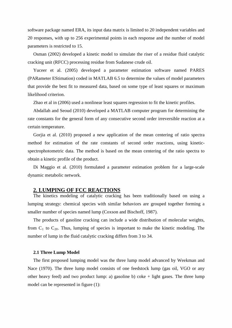
2.1 Three Lump Model

The first proposed lumping model was the three lump model advanced by Weekman and

Nace (1970). The three lump model consists of one feedstock lump (gas oil, VGO or any

other heavy feed) and two product lump: a) gasoline b) coke + light gases. The three lump

model can be represented in figure (1):

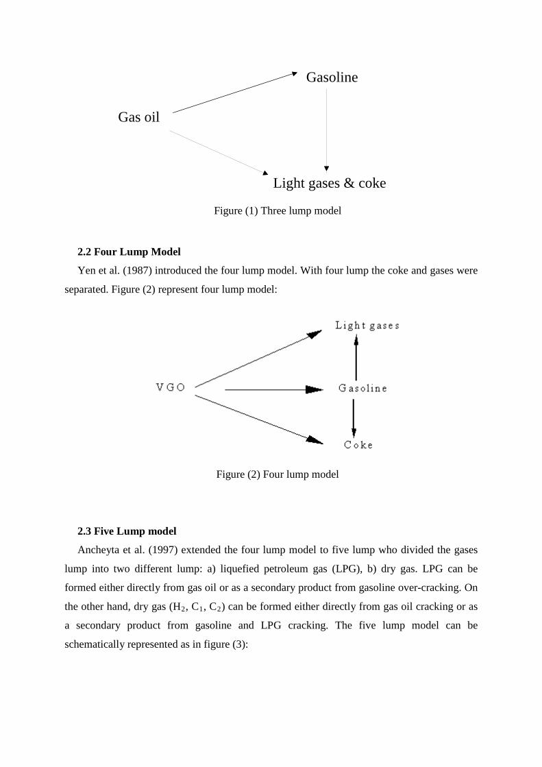
Figure (1) Three lump model

2.2 Four Lump Model

Yen et al. (1987) introduced the four lump model. With four lump the coke and gases were

separated. Figure (2) represent four lump model:

Figure (2) Four lump model

2.3 Five Lump model

Ancheyta et al. (1997) extended the four lump model to five lump who divided the gases

lump into two different lump: a) liquefied petroleum gas (LPG), b) dry gas. LPG can be

formed either directly from gas oil or as a secondary product from gasoline over-cracking. On

the other hand, dry gas (HR2R, CR1R, CR2R) can be formed either directly from gas oil cracking or as

a secondary product from gasoline and LPG cracking. The five lump model can be

schematically represented as in figure (3):

Gasoline

Light gases & coke

Gas oil

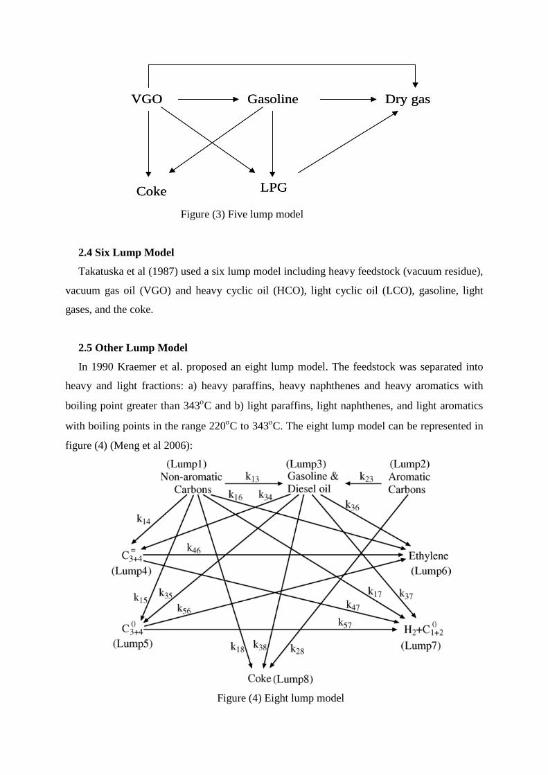
Figure (3) Five lump model

2.4 Six Lump Model

Takatuska et al (1987) used a six lump model including heavy feedstock (vacuum residue),

vacuum gas oil (VGO) and heavy cyclic oil (HCO), light cyclic oil (LCO), gasoline, light

gases, and the coke.

2.5 Other Lump Model

In 1990 Kraemer et al. proposed an eight lump model. The feedstock was separated into

heavy and light fractions: a) heavy paraffins, heavy naphthenes and heavy aromatics with

boiling point greater than 343P

οPC and b) light paraffins, light naphthenes, and light aromatics

with boiling points in the range 220P

οPC to 343P

οPC. The eight lump model can be represented in

figure (4) (Meng et al 2006):

Figure (4) Eight lump model

VGO Gasoline Dry gas

Coke LPG

VGO Gasoline Dry gas

Coke LPG

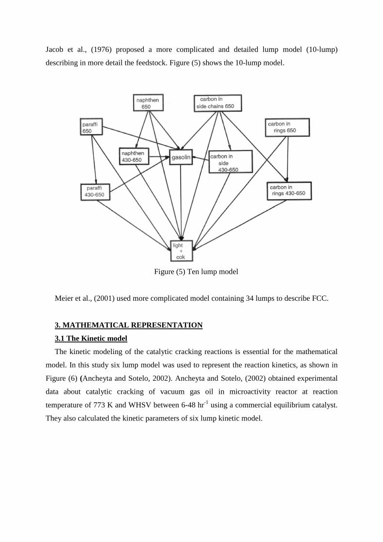
Jacob et al., (1976) proposed a more complicated and detailed lump model (10-lump)

describing in more detail the feedstock. Figure (5) shows the 10-lump model.

Figure (5) Ten lump model

Meier et al., (2001) used more complicated model containing 34 lumps to describe FCC.

3. MATHEMATICAL REPRESENTATION

3.1 The Kinetic model

The kinetic modeling of the catalytic cracking reactions is essential for the mathematical

model. In this study six lump model was used to represent the reaction kinetics, as shown in

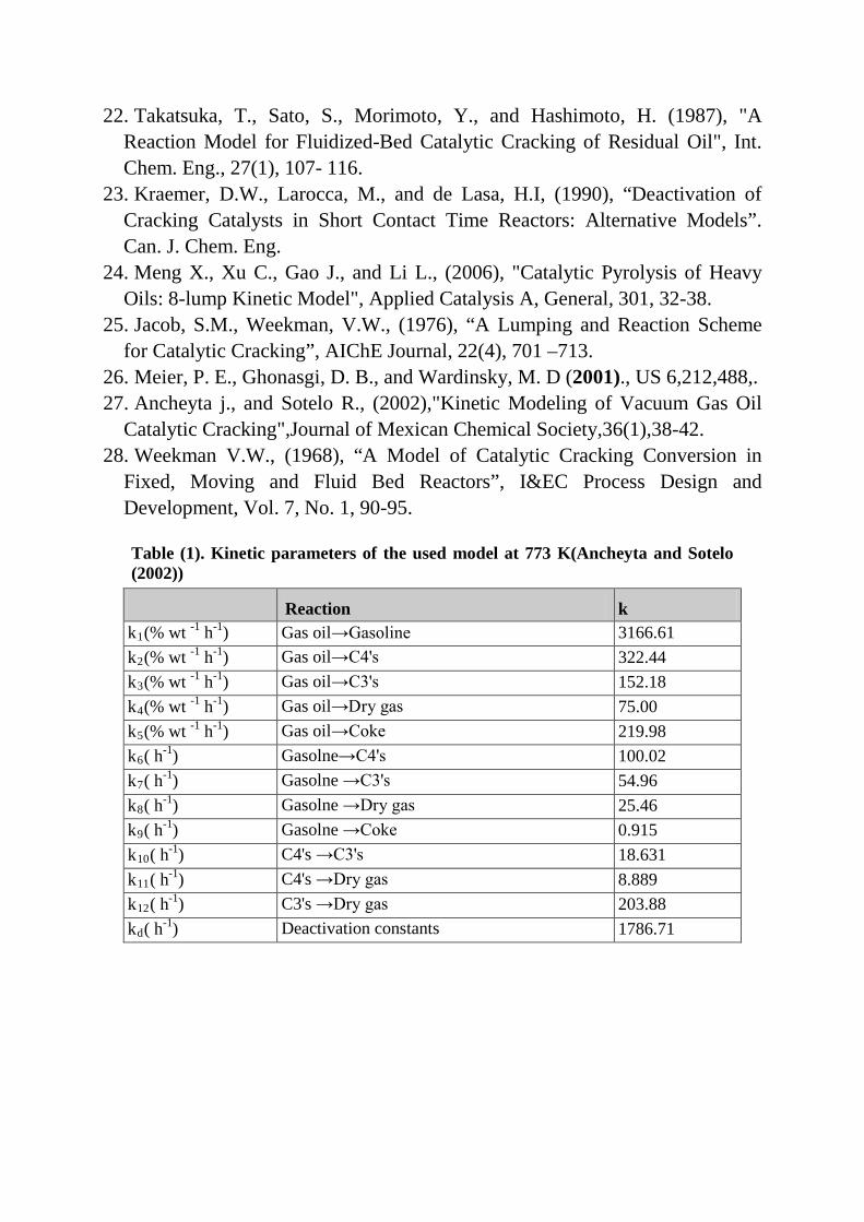
Figure (6) (Ancheyta and Sotelo, 2002). Ancheyta and Sotelo, (2002) obtained experimental

data about catalytic cracking of vacuum gas oil in microactivity reactor at reaction

temperature of 773 K and WHSV between 6-48 hrP

-1P using a commercial equilibrium catalyst.

They also calculated the kinetic parameters of six lump kinetic model.

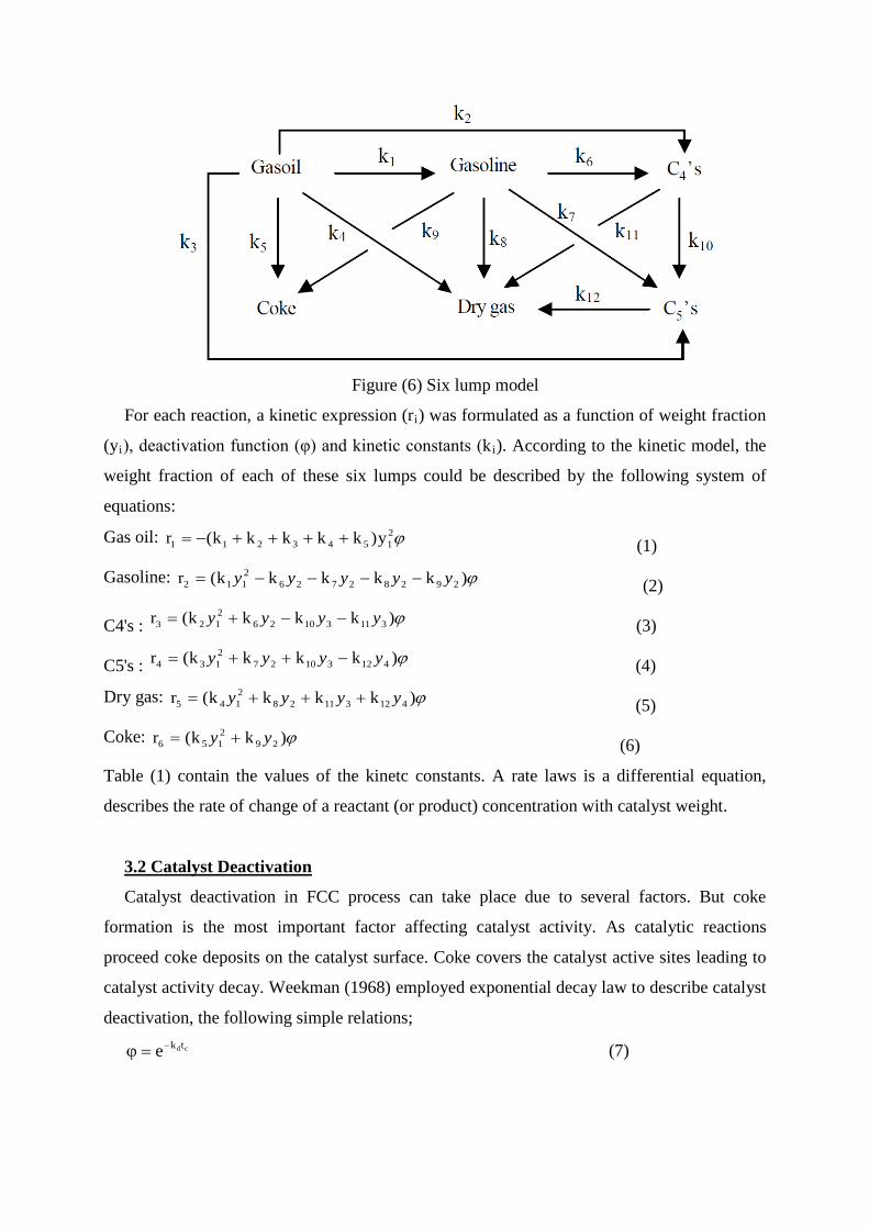
Figure (6) Six lump model

For each reaction, a kinetic expression (rRiR) was formulated as a function of weight fraction

(yRiR), deactivation function (φ) and kinetic constants (kRiR). According to the kinetic model, the

weight fraction of each of these six lumps could be described by the following system of

equations:

Gas oil: ϕ21543211 y)kkkkk(r ++++−= (1)

Gasoline: ϕ)kkkkk(r 292827262112 yyyyy −−−−= (2)

C4's : ϕ)kkkk(r 311310262123 yyyy −−+= (3)

C5's : ϕ)kkkk(r 412310272134 yyyy −++= (4)

Dry gas: ϕ)kkkk(r 412311282145 yyyy +++= (5)

Coke: ϕ)kk(r 292156 yy += (6)

Table (1) contain the values of the kinetc constants. A rate laws is a differential equation,

describes the rate of change of a reactant (or product) concentration with catalyst weight.

3.2 Catalyst Deactivation

Catalyst deactivation in FCC process can take place due to several factors. But coke

formation is the most important factor affecting catalyst activity. As catalytic reactions

proceed coke deposits on the catalyst surface. Coke covers the catalyst active sites leading to

catalyst activity decay. Weekman (1968) employed exponential decay law to describe catalyst

deactivation, the following simple relations; cdtke−=ϕ (7)

3.3 Concentration-Catalyst Weight Data

Due to the lack in the eperimental data concerning with fluid catalytic cracking, a

mathematical representation was build to generate concentration-catalyst weight data points

using six lump reaction rates. The follwing assumptions were used:.

1- Plug flow within the reactor.

2- Axial dispersion in the reactor is negligible.

3- All reactions are first order except gas oil cracking reaction which assumed to be second

order.

4- Catalyst activity decay according to exponential decay law.

5- The feed does not contain a coke.

6- Isothermal reactor temperature.

The simulltaneous first order differential differential equations (1 to 6) with catalyst

deactivation equation (7), were integrated numerically using fourth order Runge-Kutta

method with the following initial boundary conditions.

0y,0y,0y,0y,0y,1y 654321 ====== In the mathematical model, the reaction temperature was taken as 773 K and WHSV 48 hrP

-

1P. Table (2) contains the generated concentrations versus catalyst weight data of six lump

fluidized catalytic cracking reactions.

3.4 Parameter Identification

Different number of data points was used to predict parameters of reaction kinetic. The

kinetic model was predicted using data obtained in table (2) at a significant temperature 773

K. The following steps were used to calculate parameters of reaction kinetic:

1. The first step is determining the rate constants of the reactions by getting the

concentration difference for each catalyst weight interval depending on selected number of

points using the following equation:

Wcyr i

i ∆∆

=−

(8)

2. Choose an initial guess for the k values.

3. Depending on assumed k values and using equations (1-7), simulation of the kinetic

reactions is performed.

4. Updating the values of the assume k values using simplex search method.

5. The predicted values are compared with experimental ones at each measured point. All

deviations between experimental and calculated values are squared and summed up to form an

objective function F:

𝐹𝐹 = ∑ ∑ (𝑦𝑦𝑒𝑒𝑒𝑒𝑒𝑒 𝑖𝑖 − 𝑦𝑦𝑐𝑐𝑐𝑐𝑐𝑐 𝑖𝑖)2𝑁𝑁𝑗𝑗=1

𝑛𝑛𝑖𝑖=1 (9)

Where the 𝑦𝑦𝑒𝑒𝑒𝑒𝑒𝑒 𝑖𝑖 ,𝑦𝑦𝑐𝑐𝑐𝑐𝑐𝑐 𝑖𝑖 are the input (or experimental) and concentration values of species

i at catalyst weights Wc, n is the number of species and N is the number of input data points.

For each set of input points, the new value of F is calculated. The rate constants

corresponding to the minimum F are stored and considered as improved rate constants.

The Arrhenius equation represents the dependence of the reaction rate constant k on the

temperature. With this equation from two measuring points in different temperatures the

activation energy (ERAR) of the reaction could be calculated.

−=

T.REexp.kk A

0 (10)

3.5 Software

All calculations in this paper were performed using Matlab 7.0 software. The ode23

command was used to integrate simultaneous ordinary differential equations numerically

using fourth-order Runge-Kutta algorithm, while fmincon command was used to estimate the

kinetic parameters based on minimization the objective function F, which subject to a

nonlinear constraint in which k values must be positive (greater than 0).

4. RESULTS AND DISCUSSION 4.1 Reaction Kinetic

Table (3) contains the predicted reaction rate constants using different number of points.

It's clear from table (3) that, increasing the number of input data points will decrease the error

between model k values and predicted k values. The predicted reaction rate constants in Table

(3) were used in simulation and the simulation results were compared with input data points.

Figures (8, 9, 10, 11, 12 and 13) represent the predicted results using different input points (2,

3, 5, 6, 11 and 21 respectively).

In Figure (8), it's clear that using two data points (initial and final) will show fair

representation to input points. Increasing the number of data points such as in figures (9 to

13), enhanced the representation of input points.

Figure (10) shows that acceptable predicted results could be reached out in spite of huge

difference in Table (3) between the model k values and predicted k values that depending on 5

points.

Using 11 data points such as in figure (12) shows that the observed data fits the input data

very well.

Further increasing of input data points to 21 points such as in Figure ((13) shows excellent

agreement between the model predictions and input data points.

Finally, it can be concluded that, higher than 11 to 21 data points are required for good

representing of the reaction kinetic in any complex system.

5. CONCLUSION In this study, constrained non linear least square method with the aid of quasi-Newton

method was used for determining the rate constants of six lump fluidized catalytic cracking

reactions. The results showed that:-

• Increasing the number of input data points will enhance the accuracy of predicted

kinetic parameters. Accurate reaction kinetic could be described using 11 to 21 points.

• The lower accuracy reaction rate could be determined depending on two points (initial

and final).

• The same concentration behavior could be obtained using different values of the rate

constants.

• Also the results showed that the proposed programs are very efficient, fast and accurate

tools to determine the rate constants of any complex reaction at a certain temperature.

The proposed program could be modified to simulate any kinetic reaction, of any number

of components or lump such as reforming reaction kinetic.

Nomenclature

E: Activation energy ( j/mol )

kRiR: Rate constant ( wt% /hr )

kR0R: Pre-exponential factor ( wt% /hr )

kRdR: Deactivation constant ( hrP

-1P )

R: Gas law constant ( 8.314 J/mol·K )

rRiR: Rate of reaction (wt%/hr.gm catalyst )

T: Temperature ( K )

tc: Catalyst residence time ( hr )

Wc: Catalyst weight ( k )

yR1R: Weight fraction of residual oil ( wt% )

yR2R: Weight fraction of heavy fuel oil ( wt% )

yR3R: Weight fraction of light fuel oil ( wt% )

yR4R: Weight fraction of gasoline ( wt% )

yR5R: Weight fraction of liquefied petroleum gas ( wt% )

yR6R: Weight fraction of dry gas ( wt% )

φ: Deactivation function (-)

REFERENCES

1. Han, I. S., and Chung, C. B., (2001), "Dynamic Modeling and Simulation of a Fluidized Catalytic Cracking Process", Chem. Eng. Sci., 56, 1951-1971.

2. Subramanya V. N., Saket L. J., and Vivek V. R., (2005), "Modeling of Vaporization and Cracking of Liquid Oil Injected in a Gas-Solid Riser", Chem. Eng. Sci., 60, 6049-6066.

3. Gupta, R.K., Kumar, K., and Srivastava, V.K., (2007), "A New Generic Approach for the Modeling of Fluid Catalytic Cracking (FCC) Riser Reactor, Chem. Eng. Sci., 62, 4510-4528.

4. Heydari M., AleEbrahim H., and Dabir B., (2010), " Study of Seven-Lump Kinetic Model in the Fluid Catalytic Cracking Unit" American Journal of Applied Sciences, 7 (1), 71-76.

5. Weekman, V.W., (1974), “Laboratory Reactors and Their Limitations”, AIChE, 20 (5), 833-840.

6. Sunderland, P., (1976), “An Assessment of Laboratory Reactors for Heterogeneously Catalyzed Vapor Phase Reactions”, Trans. Instn. Chem. Engrs., 54, 135.

7. Hirmajer, T., Balsa-Canto E. and Banga J. R., (2009), "DOTcvpSB, a software toolbox for dynamic optimization in systems biology". BMC Bioinformatics 10, 199.

8. Brooke, A., Kendrick, D., Meeraus, A., and Raman, R., (1997). "GAMS Release" 2.25, Version 92, Language Guide.

9. Ancheyta, J.J., Lopez, I.H., Aguilar, R.E., and Moreno, M.J. (1997), "A Strategy for Kinetic Parameter Estimation in the Fluid Catalytic Cracking Process", Ind. Eng. Chem. Res., 36, 5170-5174.

10. Arx, K. B. V., Manock, J. J., Scott W. H., and Messina, M., (1998),"Using Limited Concentration Data for the Determination of Rate Constants with the Genetic Algorithm. Environ. Sci. Technol., 32 (20), 3207–3212.

11. Cai R., Wu X., Liu Z., and Ma W., (1999),"Kinetic Analysis of Consecutive Reactions Using a Non-Linear Least-Squares Error-Compensation Algorithm", Analyst, 124, 751–754.

12. Zamostny, P. and Z. Belohlav, (1999), "A Software for Regression Analysis of Kinetic Data", Computers & Chemistry, 23, 479.

13. Osman A. M., (2002), "Advanced Process Design of Residue Fluid Catalytic Cracking Unit, MSC thesis, University of Technology

14. Yuceer M., Atasoy I., and Berber R., (2005),"An Integration Based Optimization Approach for Parameter Estimation in Dynamic Models", European Symposium on Computer Aided Process Engineering-15.

15. Zhao, Y., Wang, G., Li, W., and Zhu, Z., (2006),"Determination of Reaction Mechanism and Rate Constants of Alkaline Hydrolysis of Phenyl Benzoate in Ethanol–Water Medium by Nonlinear Least Squares Regression", Chemometrics and Intelligent Laboratory Systems, 82(1), 193-199.

16. Abdallah L. A. M. and Seoud A. A., (2006), "Determination of the Rate Constants for a Consecutive Second Order Irreversible Chemical Reaction Using MATLAB Toolbox", European Journal of Scientific Research, 41 (3), 412-419.

17. Gorjia S., Bahrama M., and Golshanb A., (2010), "Estimation of the Rate Constants of Second Order Reactions Using Mean Centering of Ratio Spectra" J. Iran. Chem. Soc., Vol. 7, No. 4, 946-956.

18. Di Maggio J., Diaz Ricci J. C. and Soledad Diaz M., (2010), "Parameter Estimation in Kinetic Models for Large Scale Metabolic Networks with Advanced Mathematical Programming Techniques", 20th European Symposium on Computer Aided Process Engineering – ESCAPE.

19. Coxon, P.G., and Bischoff, K.B. (1987), "Lumping Strategy, 1. Introduction Techniques and Application of Cluster Analysis", Ind. Eng. Chem. Res., 26, 1239-1248.

20. Weekman, V.W., and Nace, D.M., (1970), “Kinetics of Catalytic Cracking Selectivity in Fixed, Moving and Fluid-bed Reactors”, AIChE, 16, 397-404.

21. Yen, L., Wrench, R., and Ong, A., (1987),”Reaction Kinetic Correlation for Predicting Coke Yield in Fluid Catalytic Cracking”. Presented at the Katalistisks’ 8P

thP Annual Fluid Catalytic Cracking Symposium, Budapest,

Hungary.

22. Takatsuka, T., Sato, S., Morimoto, Y., and Hashimoto, H. (1987), "A Reaction Model for Fluidized-Bed Catalytic Cracking of Residual Oil", Int. Chem. Eng., 27(1), 107- 116.

23. Kraemer, D.W., Larocca, M., and de Lasa, H.I, (1990), “Deactivation of Cracking Catalysts in Short Contact Time Reactors: Alternative Models”. Can. J. Chem. Eng.

24. Meng X., Xu C., Gao J., and Li L., (2006), "Catalytic Pyrolysis of Heavy Oils: 8-lump Kinetic Model", Applied Catalysis A, General, 301, 32-38.

25. Jacob, S.M., Weekman, V.W., (1976), “A Lumping and Reaction Scheme for Catalytic Cracking”, AIChE Journal, 22(4), 701 –713.

26. Meier, P. E., Ghonasgi, D. B., and Wardinsky, M. D (2001)., US 6,212,488,. 27. Ancheyta j., and Sotelo R., (2002),"Kinetic Modeling of Vacuum Gas Oil

Catalytic Cracking",Journal of Mexican Chemical Society,36(1),38-42. 28. Weekman V.W., (1968), “A Model of Catalytic Cracking Conversion in

Fixed, Moving and Fluid Bed Reactors”, I&EC Process Design and Development, Vol. 7, No. 1, 90-95. Table (1). Kinetic parameters of the used model at 773 K(Ancheyta and Sotelo (2002))

Reaction k kR1R(% wt P

-1P hP

-1P) Gas oil→Gasoline 3166.61

kR2R(% wt P

-1P hP

-1P) Gas oil→C4's 322.44

kR3R(% wt P

-1P hP

-1P) Gas oil→C3's 152.18

kR4R(% wt P

-1P hP

-1P) Gas oil→Dry gas 75.00

kR5R(% wt P

-1P hP

-1P) Gas oil→Coke 219.98

kR6R( hP

-1P) Gasolne→C4's 100.02

kR7R( hP

-1P) Gasolne →C3's 54.96

kR8R( hP

-1P) Gasolne →Dry gas 25.46

kR9R( hP

-1P) Gasolne →Coke 0.915

kR10R( hP

-1P) C4's →C3's 18.631

kR11R( hP

-1P) C4's →Dry gas 8.889

kR12R( hP

-1P) C3's →Dry gas 203.88

kRdR( hP

-1P) Deactivation constants 1786.71

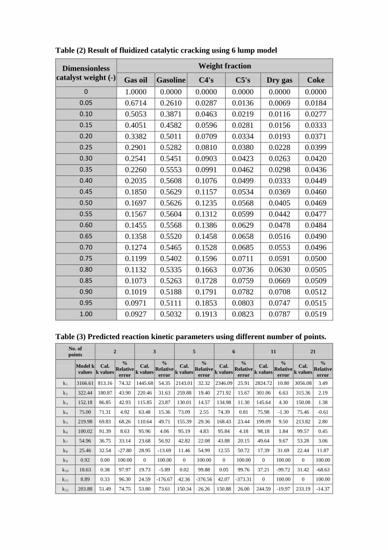
Table (2) Result of fluidized catalytic cracking using 6 lump model

Dimensionless catalyst weight (-)

Weight fraction

Gas oil Gasoline C4's C5's Dry gas Coke 0 1.0000 0.0000 0.0000 0.0000 0.0000 0.0000

0.05 0.6714 0.2610 0.0287 0.0136 0.0069 0.0184 0.10 0.5053 0.3871 0.0463 0.0219 0.0116 0.0277 0.15 0.4051 0.4582 0.0596 0.0281 0.0156 0.0333 0.20 0.3382 0.5011 0.0709 0.0334 0.0193 0.0371 0.25 0.2901 0.5282 0.0810 0.0380 0.0228 0.0399 0.30 0.2541 0.5451 0.0903 0.0423 0.0263 0.0420 0.35 0.2260 0.5553 0.0991 0.0462 0.0298 0.0436 0.40 0.2035 0.5608 0.1076 0.0499 0.0333 0.0449 0.45 0.1850 0.5629 0.1157 0.0534 0.0369 0.0460 0.50 0.1697 0.5626 0.1235 0.0568 0.0405 0.0469 0.55 0.1567 0.5604 0.1312 0.0599 0.0442 0.0477 0.60 0.1455 0.5568 0.1386 0.0629 0.0478 0.0484 0.65 0.1358 0.5520 0.1458 0.0658 0.0516 0.0490 0.70 0.1274 0.5465 0.1528 0.0685 0.0553 0.0496 0.75 0.1199 0.5402 0.1596 0.0711 0.0591 0.0500 0.80 0.1132 0.5335 0.1663 0.0736 0.0630 0.0505 0.85 0.1073 0.5263 0.1728 0.0759 0.0669 0.0509 0.90 0.1019 0.5188 0.1791 0.0782 0.0708 0.0512 0.95 0.0971 0.5111 0.1853 0.0803 0.0747 0.0515 1.00 0.0927 0.5032 0.1913 0.0823 0.0787 0.0519

Table (3) Predicted reaction kinetic parameters using different number of points.

No. of points 2 3 5 6 11 21

Model k values

Cal. k values

% Relative

error

Cal. k values

% Relative

error

Cal. k values

% Relative

error

Cal. k values

% Relative

error

Cal. k values

% Relative

error

Cal. k values

% Relative

error kR1 3166.61 813.16 74.32 1445.68 54.35 2143.01 32.32 2346.09 25.91 2824.72 10.80 3056.08 3.49

kR2 322.44 180.87 43.90 220.46 31.63 259.88 19.40 271.92 15.67 301.06 6.63 315.36 2.19

kR3 152.18 86.85 42.93 115.85 23.87 130.01 14.57 134.98 11.30 145.64 4.30 150.08 1.38

kR4 75.00 71.31 4.92 63.48 15.36 73.09 2.55 74.39 0.81 75.98 -1.30 75.46 -0.61

kR5 219.98 69.83 68.26 110.64 49.71 155.39 29.36 168.43 23.44 199.09 9.50 213.82 2.80

kR6 100.02 91.39 8.63 95.96 4.06 95.19 4.83 95.84 4.18 98.18 1.84 99.57 0.45

kR7 54.96 36.75 33.14 23.68 56.92 42.82 22.08 43.88 20.15 49.64 9.67 53.28 3.06

kR8 25.46 32.54 -27.80 28.95 -13.69 11.46 54.99 12.55 50.72 17.39 31.69 22.44 11.87

kR9 0.92 0.00 100.00 0 100.00 0 100.00 0 100.00 0 100.00 0 100.00

kR10 18.63 0.38 97.97 19.73 -5.89 0.02 99.88 0.05 99.76 37.21 -99.72 31.42 -68.63

kR11 8.89 0.33 96.30 24.59 -176.67 42.36 -376.56 42.07 -373.31 0 100.00 0 100.00

kR12 203.88 51.49 74.75 53.80 73.61 150.34 26.26 150.88 26.00 244.59 -19.97 233.19 -14.37

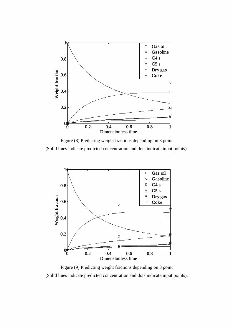
Figure (8) Predicting weight fractions depending on 3 point

(Solid lines indicate predicted concentration and dots indicate input points).

Figure (9) Predicting weight fractions depending on 3 point

(Solid lines indicate predicted concentration and dots indicate input points).

0 0.2 0.4 0.6 0.8 10

0.2

0.4

0.6

0.8

1

Dimensionless time

Wei

ght f

ract

ion

Gas oilGasolineC4 sC5 sDry gasCoke

0 0.2 0.4 0.6 0.8 10

0.2

0.4

0.6

0.8

1

Dimensionless time

Wei

ght f

ract

ion

Gas oilGasolineC4 sC5 sDry gasCoke

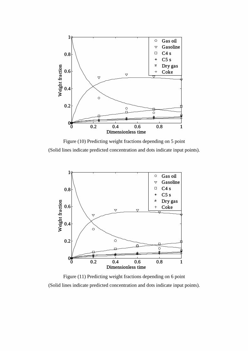
Figure (10) Predicting weight fractions depending on 5 point

(Solid lines indicate predicted concentration and dots indicate input points).

Figure (11) Predicting weight fractions depending on 6 point

(Solid lines indicate predicted concentration and dots indicate input points).

0 0.2 0.4 0.6 0.8 10

0.2

0.4

0.6

0.8

1

Dimensionless time

Wei

ght f

ract

ion

Gas oilGasolineC4 sC5 sDry gasCoke

0 0.2 0.4 0.6 0.8 10

0.2

0.4

0.6

0.8

1

Dimensionless time

Wei

ght f

ract

ion

Gas oilGasolineC4 sC5 sDry gasCoke

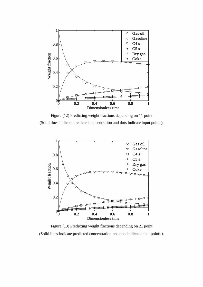
Figure (12) Predicting weight fractions depending on 11 point

(Solid lines indicate predicted concentration and dots indicate input points).

Figure (13) Predicting weight fractions depending on 21 point

(Solid lines indicate predicted concentration and dots indicate input points).

0 0.2 0.4 0.6 0.8 10

0.2

0.4

0.6

0.8

1

Dimensionless time

Wei

ght f

ract

ion

Gas oilGasolineC4 sC5 sDry gasCoke

0 0.2 0.4 0.6 0.8 10

0.2

0.4

0.6

0.8

1

Dimensionless time

Wei

ght f

ract

ion

Gas oilGasolineC4 sC5 sDry gasCoke

حساب ثوابت ميكانيكية التفاعالت المعقدة باستخدام لغة ماتالب

د. زيدون محسن شكور/ قسم الهندسة الكيمياوية /بغداد الجامعة التكنولوجية

dr_zaidoon@yahoo.com الخالصة :

عملية حساب ثوابت التفاعالت الكيمياوية تكون عملية معقدة ومستهلكة للوقت. الهدف من هذا البحث هو:

باستخدام لغة ماتالب لحساب ثوابت التفاعالت الي نظام معقد من التفاعالت والي درجة تطوير برنامج •

حرارة.

دراسة تاثيرعدد النقاط المدخلة للبرنامج على دقة حساب ثوابت التفاعالت. •في هذا البحث تم دراسة تفاعالت التكسير المحفز. حيث تم عمل موديل رياضي أليجاد تراكيز المواد مع وزن العامل

المساعد باستخدام ميكانيكية تفاعل من ستة مواد. هذه البيانات تم اعتبارها كبيانات عملية وتم استخدامها الحقا اليجاد ثوابت

التفاعالت.

باستخدام عدد مختلف من النقاط لكل مرة تم حساب ثوابت معدل التفاعل بطريقة تقليل مجموع مربع الخطأ بين النقاط

المدخلة للموديل والنقاط المحسوبة من الموديل. حيث تم تقليل مجموع مربع الخطأ باستخدام طريقة التكرار والتحقق.

هذا البحث اجاب عن التسأول الموجود لدى اي باحث وهو هل يمكن حساب معدل التفاعل الي تفاعل معقد باالعتماد

وصف ضعيف لمعدالت التفاعالت باالعتماد على نقطتين. على نقطتين( بداية ونهاية)؟ . حيث كانت االجابة انه يمكن ايجاد

وتبين ان البرنامج الرياضي المطور فعال وسريع ودقيق في حساب ثوابت معدالت التفاعالت الي نظام من التفاعالت

وللحصول على وصف جيد لميكانيكية اي تفاعل يجب الحصول على عدد من النقاط العملية المعقدة وباية درجة حرارية.

نقطة.21 الى 11يتراوح بين

الكلمات الداله : التكسير الحراري المحفز ، معدل التفاعل، ثوابت،افضل، ماتالب