Embed Size (px)
Citation preview
3rd International Symposium on Advances in Civil and Environmental Engineering Practices for Sustainable Development (ACEPS – 2015)
Estimation of Leachate Generation Using HELP Model in an Open Dumpsite in Sri Lanka
N. M. Muthukumara1, P.P.U. Kumarasinghe1, M.I.M. Mowjood2, M. Nagamori3,Y. Isobe3, Y. Watanabe3, Y.Inoue4,G.B.B. Herath5and K. Kawamoto4
1Postgraduate Institute of Agriculture University of Peradeniya
Peradeniya, Sri Lanka
2Department of Agricultural Engineering Faculty of Agriculture University of Peradeniya Peradeniya, Sri Lanka
3Center for Environmental Science in Saitama
914 Kamitanadare, Kazo, Saitama 347-0115, Japan
4Institute for Environmental Science and Technology Graduate School of Science and Engineering Saitama University
255 Shimo-Okubo, Sakura-ku, Saitama 338-8570, Japan
5Department of Civil Engineering Faculty of Engineering University of Peradeniya Peradeniya, Sri Lanka
Email: [email protected]
Abstract: Managing leachate is one of the problems associated with municipal solid waste landfills. Leachate generation highly varies with type of waste, climate, site and surface condition. Several mathematical computer models have been used for prediction of leachate for controlled sanitary landfills. However, the prediction of leachate for an open dumpsite is rarely reported. The applicability of Hydrologic Evaluation of Landfill Performance (HELP) model which is based on water balance method was evaluated in this study for Udapalatha open dump site in the Central Province, Sri Lanka. Input weather data (rainfall, temperature, Relative Humidity, wind velocity, solar radiation) and site specific data (area, depth, profile characteristics) were obtained from nearby weather station and site investigation, respectively. Model output leachate was validated (quasi) with changes in groundwater level in percussion boreholes which were installed at the dump site and monitored from May 2013.The leachate generation was 2759 mm when the rainfall was 3270 mm in 2013. Thus, 84% of the precipitation is contributed to leachate annually. The trends in temporal changes of water level in monitoring well and estimated leachate with rainfall were similar. Monthly leachate generation shows that the leachate is more than rainfall in few months where heavy rain was recorded in the previous month. This may be due to the release of water stored in the waste layer in the previous month. HELP model satisfactorily produce the annual and monthly leachate in the open dump site tested. Keywords: HELP model, Leachate, Municipal solid waste, Open dumpsite.
1. INTRODUCTION
Leachate is formed by percolation of rainfall through an open solid waste landfill or through the cap of a completed site when the refuse moisture content exceeds its field capacity (El-fadelet al 2010). Leachate contains of organic and inorganic compounds, microorganisms, humic, fulvic substances, carcinogenic materials thus, a source of pollutant for surface and groundwater contamination. One of the problems associated with landfill is managing the leachate generation. The quantity of landfill leachate can exhibit considerable temporal variations due to many factors such as climate, refuse characteristics and internal process of landfill. Climate is the main factor that governs the
176

3rd International Symposium on Advances in Civil and Environmental Engineering Practices for Sustainable Development (ACEPS – 2015)
Cook, P. G., & Walker, G. R. (1992). Depth Profiles of Electrical Conductivity from Linear Combinations of Electromagnetic Induction Measurements. Soil Science Society of America Journal, 56, 1015-1022. Geophex Limited 2004,viewed9 September 2014, http://www.geophex.com/How%20to%20Survey%20GEM_2.htmlGrellier, S., K.R. Reddy, J. Gangathulasi, R. adib and C. C. Peters (2007) Correlation between Electrical Resistivity and moisture content of Municipal Solid Waste in Bioreactor landfill, Geotechnical Special Publication, ASCE Press Reston, Virginia, USA. Letellier, M. (2012),A Practical Assessment of Frequency Electromagnetic Inversion in a Near Surface Geological Environment. Bachelor’s thesis, Lund University, Department of Geology, Sweden. McDowell, P.W., Barker, R.D., Butcher, A.P., Culshaw, M.G., Jackson, P.D., McCann, D.M., Skipp, B.O., Matthews, S.L., Arthur, J.C. (2002),Geophysics in Engineering Investigation, Construction industry research and information association(CIRIA), London.McGinnis, R.N., Sandberg, S.K., Green, R.T., Ferrill, D.A. (2011),Review of Geophysical Methods for Site Characterization of Nuclear Waste Disposal Sites, U.S. Nuclear Regulatory Commission, Texas. Sharma, H.D., Reddy, K.R. (2004),Geoenvironmental Engineering, John Wiley & Sons, Inc., New Jersey. Wijesekara, H.R., De Silva, S.N., Wijesundara, D.T., Basnayake, B.F., Vithanage, M.S. (2014),Leachate Plume Delineation and Lithologic Profiling Using Surface Resistivity in an Open Municipal Solid Waste Dumpsite, Sri Lanka, Environmental Technology,DOI:10.1080/09593330.2014.963697, pp. 1-8. Won, I.J., Keiswetter, D.A., Fields, G.R., Sutton, L.C. (1996),GEM-2: A New Multifrequency Electromagnetic Sensor,Journal of Environmental and Engineering Geophysics, 1(2),pp. 129-137. Zungalia, E.J., Tuck, F.C., Spariosu, D.J. (1989),Geophysical Investigations of A Ground Water Contaminant Plume-Electrical and Electromagnetic Methods. In Hatcher, K.J. (Ed) Preprints of the Georgia WateACEPS/15/A1/03r Resources Conference, Georgia,May 16 – May 17, pp. 165-168.
175
3rd International Symposium on Advances in Civil and Environmental Engineering Practices for Sustainable Development (ACEPS – 2015)
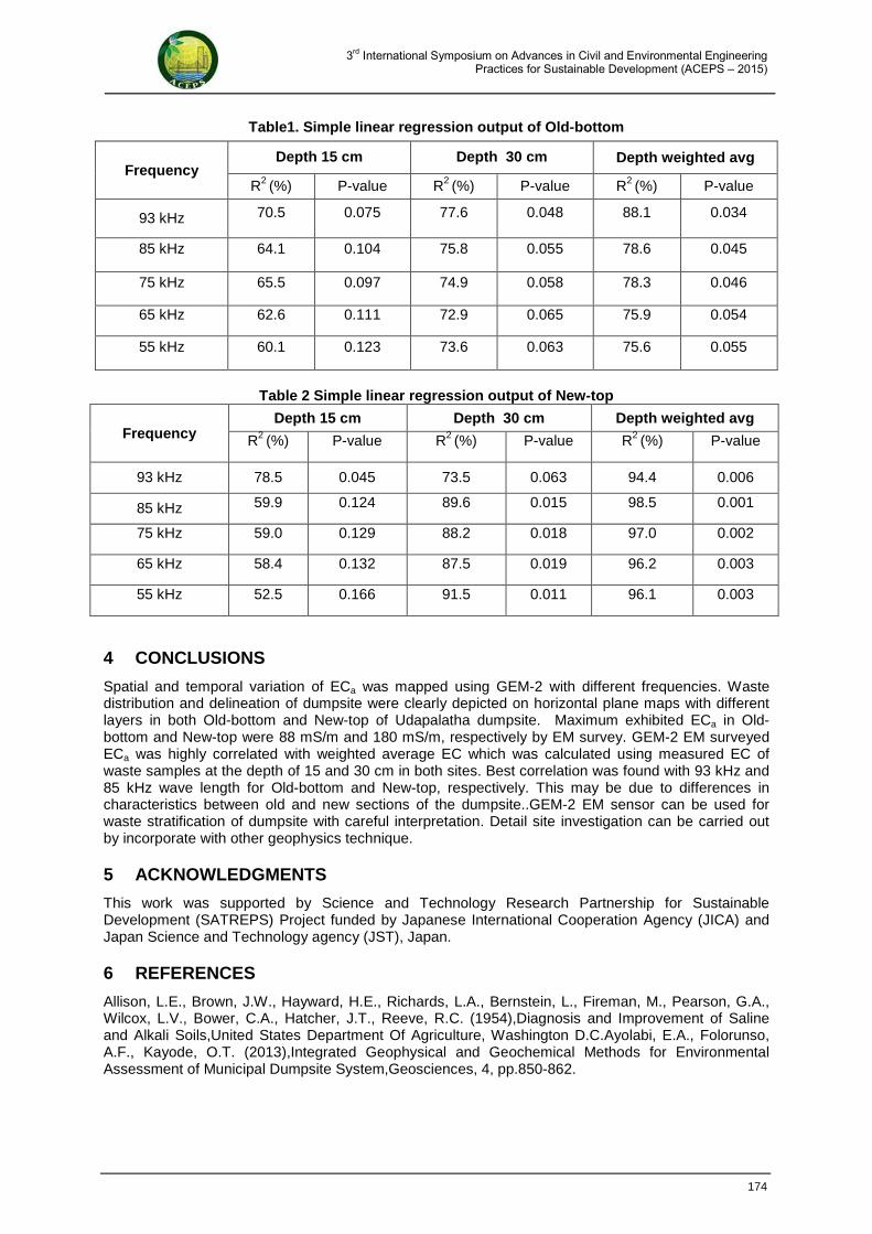
Table1. Simple linear regression output of Old-bottom
Table 2 Simple linear regression output of New-top
Frequency Depth 15 cm Depth 30 cm Depth weighted avg
R2 (%) P-value R2 (%) P-value R2 (%) P-value
93 kHz 78.5 0.045 73.5 0.063 94.4 0.006
85 kHz 59.9 0.124 89.6 0.015 98.5 0.001
75 kHz 59.0 0.129 88.2 0.018 97.0 0.002
65 kHz 58.4 0.132 87.5 0.019 96.2 0.003
55 kHz 52.5 0.166 91.5 0.011 96.1 0.003
4 CONCLUSIONS
Spatial and temporal variation of ECa was mapped using GEM-2 with different frequencies. Waste distribution and delineation of dumpsite were clearly depicted on horizontal plane maps with different layers in both Old-bottom and New-top of Udapalatha dumpsite. Maximum exhibited ECa in Old-bottom and New-top were 88 mS/m and 180 mS/m, respectively by EM survey. GEM-2 EM surveyed ECa was highly correlated with weighted average EC which was calculated using measured EC of waste samples at the depth of 15 and 30 cm in both sites. Best correlation was found with 93 kHz and 85 kHz wave length for Old-bottom and New-top, respectively. This may be due to differences in characteristics between old and new sections of the dumpsite..GEM-2 EM sensor can be used for waste stratification of dumpsite with careful interpretation. Detail site investigation can be carried out by incorporate with other geophysics technique.
5 ACKNOWLEDGMENTS
This work was supported by Science and Technology Research Partnership for Sustainable Development (SATREPS) Project funded by Japanese International Cooperation Agency (JICA) and Japan Science and Technology agency (JST), Japan.
6 REFERENCES
Allison, L.E., Brown, J.W., Hayward, H.E., Richards, L.A., Bernstein, L., Fireman, M., Pearson, G.A., Wilcox, L.V., Bower, C.A., Hatcher, J.T., Reeve, R.C. (1954),Diagnosis and Improvement of Saline and Alkali Soils,United States Department Of Agriculture, Washington D.C.Ayolabi, E.A., Folorunso, A.F., Kayode, O.T. (2013),Integrated Geophysical and Geochemical Methods for Environmental Assessment of Municipal Dumpsite System,Geosciences, 4, pp.850-862.
Frequency Depth 15 cm Depth 30 cm Depth weighted avg
R2 (%) P-value R2 (%) P-value R2 (%) P-value
93 kHz 70.5 0.075 77.6 0.048 88.1 0.034
85 kHz 64.1 0.104 75.8 0.055 78.6 0.045
75 kHz 65.5 0.097 74.9 0.058 78.3 0.046
65 kHz 62.6 0.111 72.9 0.065 75.9 0.054
55 kHz 60.1 0.123 73.6 0.063 75.6 0.055
174
3rd International Symposium on Advances in Civil and Environmental Engineering Practices for Sustainable Development (ACEPS – 2015)
Figure 5 ECa map with different frequency on 02.12.2014 (a) Old-bottom (b) New-top
3.3 Validation of GEM – 2 EM survey
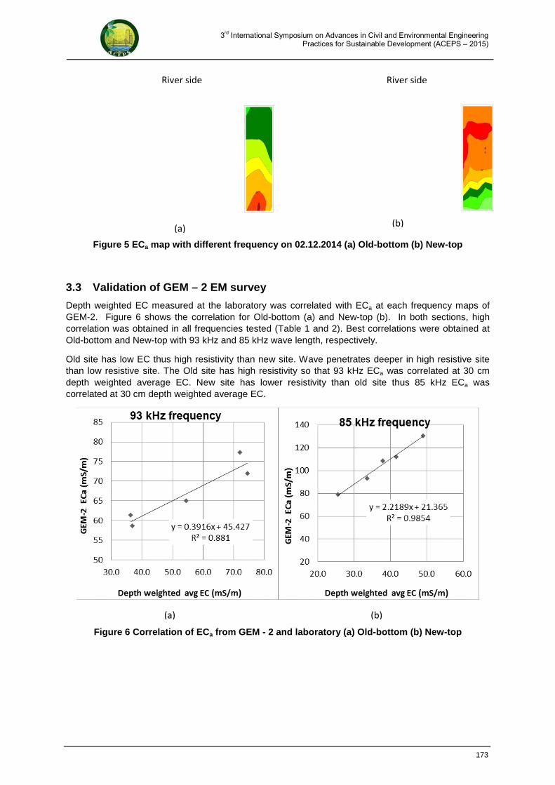
Depth weighted EC measured at the laboratory was correlated with ECa at each frequency maps of GEM-2. Figure 6 shows the correlation for Old-bottom (a) and New-top (b). In both sections, high correlation was obtained in all frequencies tested (Table 1 and 2). Best correlations were obtained at Old-bottom and New-top with 93 kHz and 85 kHz wave length, respectively.
Old site has low EC thus high resistivity than new site. Wave penetrates deeper in high resistive site than low resistive site. The Old site has high resistivity so that 93 kHz ECa was correlated at 30 cm depth weighted average EC. New site has lower resistivity than old site thus 85 kHz ECa was correlated at 30 cm depth weighted average EC.
Figure 6 Correlation of ECa from GEM - 2 and laboratory (a) Old-bottom (b) New-top
(a) (b)
(a) (b)
River side River side
173
3rd International Symposium on Advances in Civil and Environmental Engineering Practices for Sustainable Development (ACEPS – 2015)
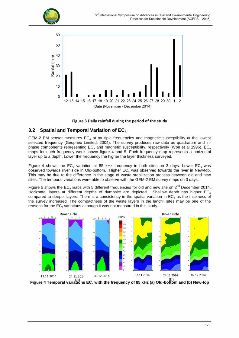
Figure 3 Daily rainfall during the period of the study
3.2 Spatial and Temporal Variation of ECa
GEM-2 EM sensor measures ECa at multiple frequencies and magnetic susceptibility at the lowest selected frequency (Geophex Limited, 2004). The survey produces raw data as quadrature and in-phase components representing ECa and magnetic susceptibility, respectively (Won et al 1996). ECa maps for each frequency were shown figure 4 and 5. Each frequency map represents a horizontal layer up to a depth. Lower the frequency the higher the layer thickness surveyed. Figure 4 shows the ECa variation at 85 kHz frequency in both sites on 3 days. Lower ECa was observed towards river side in Old-bottom. Higher ECa was observed towards the river in New-top. This may be due to the difference in the stage of waste stabilization process between old and new sites. The temporal variations were able to observe with the GEM-2 EM survey maps on 3 days.
Figure 5 shows the ECa maps with 5 different frequencies for old and new site on 2nd December 2014. Horizontal layers at different depths of dumpsite are depicted. Shallow depth has higher ECa
compared to deeper layers. There is a consistency in the spatial variation in ECa as the thickness of the survey increased. The compactness of the waste layers in the landfill sites may be one of the reasons for the ECa variations although it was not measured in this study.
Figure 4 Temporal variations ECa with the frequency of 85 kHz (a) Old-bottom and (b) New-top
(b) (a)
River side River side
172
3rd International Symposium on Advances in Civil and Environmental Engineering Practices for Sustainable Development (ACEPS – 2015)
2.2 GEM-2 Electromagnetic Survey
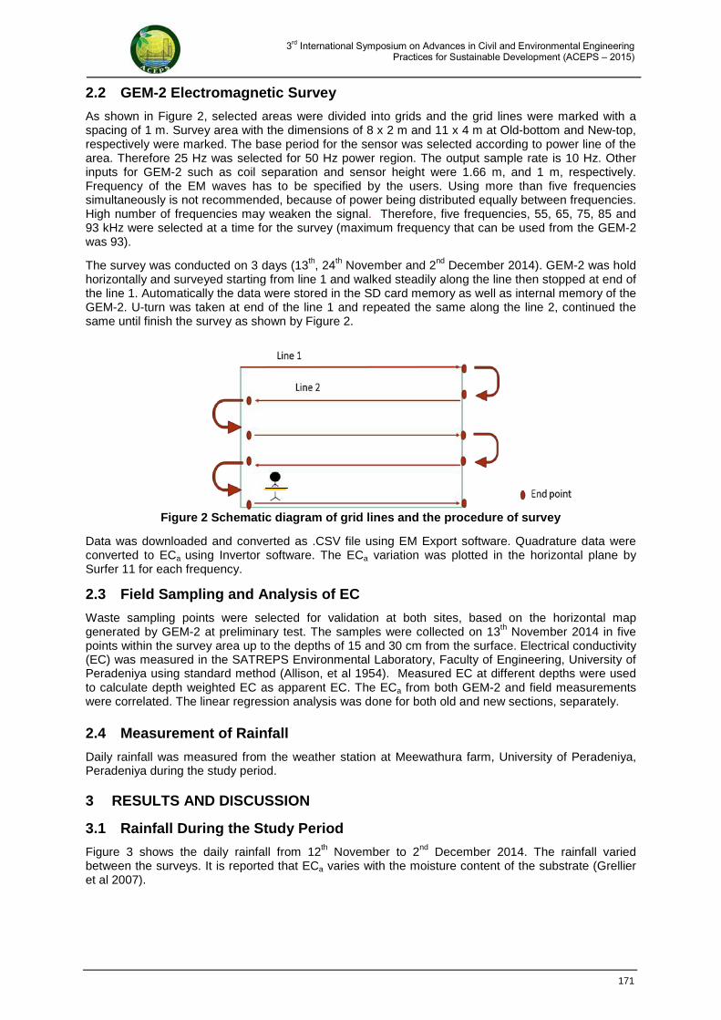
As shown in Figure 2, selected areas were divided into grids and the grid lines were marked with a spacing of 1 m. Survey area with the dimensions of 8 x 2 m and 11 x 4 m at Old-bottom and New-top, respectively were marked. The base period for the sensor was selected according to power line of the area. Therefore 25 Hz was selected for 50 Hz power region. The output sample rate is 10 Hz. Other inputs for GEM-2 such as coil separation and sensor height were 1.66 m, and 1 m, respectively. Frequency of the EM waves has to be specified by the users. Using more than five frequencies simultaneously is not recommended, because of power being distributed equally between frequencies. High number of frequencies may weaken the signal. Therefore, five frequencies, 55, 65, 75, 85 and 93 kHz were selected at a time for the survey (maximum frequency that can be used from the GEM-2 was 93).
The survey was conducted on 3 days (13th, 24th November and 2nd December 2014). GEM-2 was hold horizontally and surveyed starting from line 1 and walked steadily along the line then stopped at end of the line 1. Automatically the data were stored in the SD card memory as well as internal memory of the GEM-2. U-turn was taken at end of the line 1 and repeated the same along the line 2, continued the same until finish the survey as shown by Figure 2.
Figure 2 Schematic diagram of grid lines and the procedure of survey
Data was downloaded and converted as .CSV file using EM Export software. Quadrature data were converted to ECa using Invertor software. The ECa variation was plotted in the horizontal plane by Surfer 11 for each frequency.
2.3 Field Sampling and Analysis of EC
Waste sampling points were selected for validation at both sites, based on the horizontal map generated by GEM-2 at preliminary test. The samples were collected on 13th November 2014 in five points within the survey area up to the depths of 15 and 30 cm from the surface. Electrical conductivity (EC) was measured in the SATREPS Environmental Laboratory, Faculty of Engineering, University of Peradeniya using standard method (Allison, et al 1954). Measured EC at different depths were used to calculate depth weighted EC as apparent EC. The ECa from both GEM-2 and field measurements were correlated. The linear regression analysis was done for both old and new sections, separately.
2.4 Measurement of Rainfall
Daily rainfall was measured from the weather station at Meewathura farm, University of Peradeniya, Peradeniya during the study period.
3 RESULTS AND DISCUSSION
3.1 Rainfall During the Study Period
Figure 3 shows the daily rainfall from 12th November to 2nd December 2014. The rainfall varied between the surveys. It is reported that ECa varies with the moisture content of the substrate (Grellier et al 2007).
171
3rd International Symposium on Advances in Civil and Environmental Engineering Practices for Sustainable Development (ACEPS – 2015)
The open dumpsites have to be monitored for better management since the gas emission and leachate generation varies spatially and temporally. Conventional monitoring of MSW dumpsite required drilling, sampling and laboratory analyzing that costs and time consuming. Investigation on spatial and temporal variation is also difficult with spot measurements. In this context, the geophysical methods such as Electromagnetic (EM), Ground penetrating radar (GPR), Seismic refraction, Electrical resistivity, Gravity, Borehole geophysical logging, Induced polarization and Thermal infrared are used to monitor and evaluate the dumpsites features (McDowell, et al 2002; McGinnis, et al2011, Ayolabi, et al 2013). Geophysical methods are best options to investigate the dumpsites, because of effective sampling strategy, reduced assessment cost as reducing the number of borings/wells needed and investigating large area(Zungalia, et al 1989; Letellier, 2012; Wijesekara, et al 2014). These methods are generally used in preliminary investigations with verification of direct method. However geophysical data interpretation is quite difficult and needs special expertise (Sharma & Reddy, 2004). High initial capital investment is one of the main factors hindering the wider use of this technology in landfill survey in Sri Lanka. Apparent electrical conductivity (ECa) is the depth weighted average of the bulk soil electrical conductivity. It can be measured in both ways such as contact and non-contact methods. It is commonly measured by using EM techniques (Cook & Walker, 1992). ECa is good indicator of soil physical and chemical properties. GEM-2 is a handheld, digital, programmable, multi-frequency, broadband EM sensor which widely uses to geological, environmental and geotechnical surveys. This sensor produces EM waves at pre-set multi frequencies and receives secondary EM waves from eddy current of substrate depending on the ECa of the substrate. Thus ECa of the underneath substrate can be mapped. Open dumpsites in Sri Lanka are rarely monitored by geophysical methods, due to its availability and validation. This study was conducted to reveal the applicability of EM survey in an open dumpsite at Udapalatha.
2 METHODOLOGY
2.1 Study area
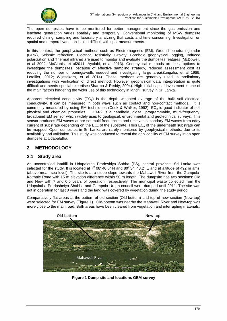
An uncontrolled landfill in Udapalatha Pradeshiya Sabha (PS), central province, Sri Lanka was selected for the study. It is located at 70 08' 40.8" N and 800 34' 43.2" E and at altitude of 492 m amsl (above mean sea level). The site is at a steep slope towards the Mahaweli River from the Gampola-Kotmale Road with 15 m elevation difference within 50 m length. The dumpsite has two sections: Old and New with 7 and 0.5 years of operation, respectively. The municipal waste collected from the Udapalatha Pradasheiya Shabha and Gampola Urban council were dumped until 2011. The site was not in operation for last 3 years and the land was covered by vegetation during the study period.
Comparatively flat areas at the bottom of old section (Old-bottom) and top of new section (New-top) were selected for EM survey (Figure 1). Old-bottom was nearby the Mahaweli River and New-top was more close to the main road. Both areas have been cleared from vegetation and interrupting materials.
Figure 1 Dump site and locations GEM survey
Mahaweli River
Old-bottom New-top
170
3rd International Symposium on Advances in Civil and Environmental Engineering Practices for Sustainable Development (ACEPS – 2015)
Electromagnetic Survey (GEM-2) for Monitoring of an Open Dumpsite in Sri Lanka
S. Kamaleswaran1, P.P.Udayagee Kumarasinghe1, M.I.M. Mowjood2, M. Nagamori3, Y. Isobe3, Y. Watanabe3,G.B.B. Herath4and K. Kawamoto5
1Postgraduate Institute of Agriculture, University of Peradeniya
Peradeniya, Sri Lanka
2Department of Agricultural Engineering, Faculty of Agriculture, University of Peradeniya Peradeniya, Sri Lanka
3Center for Environmental Science in Saitama
914 Kamitanadare, Kazo, Saitama 347-0115, Japan
4Department of Civil Engineering, Faculty of Engineering, University of Peradeniya Peradeniya, Sri Lanka
5Institute for Environmental Science and Technology
Graduate School of Science and Engineering, Saitama University 255 Shimo-Okubo, Sakura-ku, Saitama 338-8570, Japan
email: [email protected]
Abstract: Open dumping of municipal solid waste creates series of environmental and social problems. Monitoring of dumpsites is important in deciding and designing the mitigation measures to reduce the risk. Direct and continuous monitoring of dumpsite is difficult and requires time, money and labour for both sample collection and laboratory analysis. Geophysical methods such as electromagnetic (EM) technique can be used for subsurface investigation rapidly without in-situ drilling and sampling. GEM-2 is a Multi-frequency, handheld EM sensor. This produces EM waves at pre-set multi frequencies and receives secondary EM waves from eddy current of substrate depending on the apparent electrical conductivity (ECa) of the substrate. Thus ECa of the underneath substrate can be mapped. An open dumpsite in Udapaltha Pradeshiya Sabha, Central province, Sri Lanka was surveyed using GEM-2 and validated with field measurement. For validation, waste samples were collected up to 30 cm depth and electrical conductivity (EC) was measured at the laboratory and ECa was calculated. Spatial and temporal variation of ECa and delineation were clearly depicted in maps produced by GEM-2. Maximum reported ECa in Old-bottom and New-top of dump site were 88 mS/m and 180 mS/m, respectively. Measured ECa and EM surveyed ECa were correlated with simple linear regression. Best correlations were obtained at Old-bottom with 93 kHz wave length while 85 kHz for New-top. It can be concluded that EM survey is a powerful technique for dumpsite monitoring with cautious interpretation.
Keywords: Apparent electrical conductivity, Electromagnetic survey Municipal solid waste, Open dumpsite.
1 INTRODUCTION
Municipal Solid Waste (MSW) has been identified as one of the major pollution problems of the world, and become one of the major challenges in developing countries. Most common disposal method of MSW in Sri Lanka is open dumping. Wastes in dumpsites undergo decomposing processes results in several organic and inorganic substances. Most of these compounds leave the dumpsite as leachate and gas and pollute the environment.
169
3rd International Symposium on Advances in Civil and Environmental Engineering Practices for Sustainable Development (ACEPS – 2015)
5.5 pH require a minimum 5g/L NRE dosage. In all experiments the Cu adsorption was very rapid and within the initial 10 minutes, over 99% removal efficiency achieved for 5g/L NRE dosage. As an overall conclusion, the above studies indicate that Natural Red Earth found in North-Western coastal areas of Sri Lanka is a promising candidate material to remove Cu from aqueous solutions especially from low concentration solutions such as leachate contaminated groundwater. Further studies are being carried out with NRE to check its potential to remove other heavy metals found in leachate and to develop a prototype PRB unit using the Natural Red Earth. 5. ACKNOWLEDGEMENTS
The authors would like to express their sincere gratitude the JICA and JST for financially supporting this research under its Science and Technology Research Partnership for Sustainable Development (SATREPS) project.
6. REFERENCES
Ajmal,M., Khan, A.H., Ahmad, S., Role of sawdust in the removal of copper (II) from industrial wastes, Water Resources, 32/10 (1998) 3085-3091. Arneth, J.D., Midle, G., Kerndoff, H. and Schleger, R., Waste in deposits influence on ground water quality as a tool for waste type and site selection for final storage quality, Landfill reactions and final storage quality. Baccini, P. (ed), Springer Verlag Berlin, pp.339 (1989) Cay, S., Uyamk, A., Ozasik, A., Single and binary component adsorption of copper (II) and cadmium (II) from aqueous solutions using tea-industry waste, Sep.Purif. Technol.,38/3 (2004) 273-280 Demirbas, A. (2008). Heavy metal adsorption onto agro-based waste materials: A review, Journal of Hazardous Materials, 157, 220–229 Mahatantila, K., Seike, Y. and Okumura, M. (2011). Adsorptive removal of lead(II) ion using Natural Red Earth from its iron and aluminum oxide forms, International Journal of Engineering Science and Technology, 3(2), 1655-1666. Nikagolla, C., Chandrajith, R., Weerasooriya, R. and Dissanayake, C.B. (2013). Adsorption kinetics of chromium(III) removal from aqueous solutions using natural red earth, Environ Earth Sci, 68, 641–645 Park, J.B., Lee, S.H., Lee, J.W. and Lee C.Y. (2002). Lab scale experiments for permeable reactive barriers against contaminated groundwater with ammonium and heavy metals using clinoptilolite, Journal of Hazardous Materials, B95, 65–79 Rajapaksha, A.U., Vithanage, M. and Jayarathna, C.L. (2011). Natural Red Earth as a low cost material for Arsenic removal: Kinetics and the effect of competing ions, Applied Geochemistry, 26, 648–654 Raman, N., Narayanan, D.S., (2008), Impact of Solid Waste effect on Ground Water and Soil Quality nearer to Pallavaram Solid Waste Landfill Site in Chennai, Rasayan Journal of Chemistry, Vol. 1, 04, 828-836 Sewwandi, B. G. N., Koide T., Ken K., Shoichiro H., Shingo A. and Hiroyasu S. (2012), Characterization of Landfill Leachate from Municipal Solid Waste Landfills in Sri Lanka. In: 2nd International Conference on Sustainable Built Environment, pp 21. Vithanage, M., Chandrajith, R., Bandara, A. and Weerasooriya, R. (2006). Mechanistic modeling of arsenic retention on natural red earth in simulated environmental systems, Journal of Colloid and Interface Science, 294, 265–272 Vithanage, M., Seneviratne, V., Bandara, A. and Weerasooriya, R. (2007). Arsenic binding mechanisms on natural red earth: A potential substrate for pollution control, Science of the Total Environment 379 (2007) 244–248
168
3rd International Symposium on Advances in Civil and Environmental Engineering Practices for Sustainable Development (ACEPS – 2015)
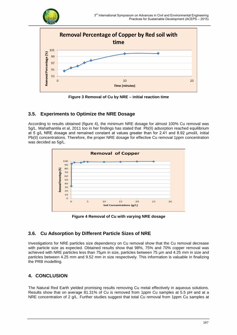
Figure 3 Removal of Cu by NRE – initial reaction time
3.5. Experiments to Optimize the NRE Dosage
According to results obtained (figure 4), the minimum NRE dosage for almost 100% Cu removal was 5g/L. Mahathantila et al, 2011 too in her findings has stated that Pb(II) adsorption reached equilibrium at 5 g/L NRE dosage and remained constant at values greater than for 2.41 and 8.92 μmol/L initial Pb(II) concentrations. Therefore, the proper NRE dosage for effective Cu removal 1ppm concentration was decided as 5g/L.
Figure 4 Removal of Cu with varying NRE dosage
3.6. Cu Adsorption by Different Particle Sizes of NRE
Investigations for NRE particles size dependency on Cu removal show that the Cu removal decrease with particle size as expected. Obtained results show that 98%, 75% and 70% copper removal was achieved with NRE particles less than 75µm in size, particles between 75 µm and 4.25 mm in size and particles between 4.25 mm and 9.52 mm in size respectively. This information is valuable in finalizing the PRB modelling. 4. CONCLUSION
The Natural Red Earth yielded promising results removing Cu metal effectively in aqueous solutions. Results show that on average 81.31% of Cu is removed from 1ppm Cu samples at 5.5 pH and at a NRE concentration of 2 g/L. Further studies suggest that total Cu removal from 1ppm Cu samples at
167
3rd International Symposium on Advances in Civil and Environmental Engineering Practices for Sustainable Development (ACEPS – 2015)
-2.000E-01
0.000E+00
2.000E-01
4.000E-01
6.000E-01
8.000E-01
1.000E+00
1.200E+00
1.400E+00
0.00 2.00 4.00 6.00 8.00 10.00
Char
ge d
ensi
ty/
Cm-2
pH
Red Soil
0.01M
0.1 M
0.001 M
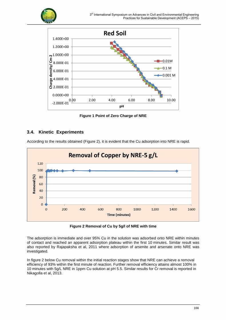
Figure 1 Point of Zero Charge of NRE
3.4. Kinetic Experiments
According to the results obtained (Figure 2), it is evident that the Cu adsorption into NRE is rapid.
Figure 2 Removal of Cu by 5g/l of NRE with time
The adsorption is immediate and over 95% Cu in the solution was adsorbed onto NRE within minutes of contact and reached an apparent adsorption plateau within the first 10 minutes. Similar result was also reported by Rajapaksha et al, 2011 where adsorption of arsenite and arsenate onto NRE was investigated. In figure 2 below Cu removal within the initial reaction stages show that NRE can achieve a removal efficiency of 93% within the first minute of reaction. Further removal efficiency attains almost 100% in 10 minutes with 5g/L NRE in 1ppm Cu solution at pH 5.5. Similar results for Cr removal is reported in Nikagolla et al, 2013.
166
3rd International Symposium on Advances in Civil and Environmental Engineering Practices for Sustainable Development (ACEPS – 2015)
were taken out at 1, 2,3,4,5, 10 and 15 minutes for analysis. The supernatant were taken to tubes immediately, centrifuged at 16,000 rpm and analyzed for remaining Cu with the AAS. 2.7 Cu Adsorption with Different Particle Sizes of NRE Particles size distribution in Red soil show only 33% of particles are less than 75µm in size. Since particle size is directly propotional to the available surface area and is an influential factor in adsorption, experiments were carried out using three particle size ranges; sizes less than 75µm, sizes between 75µm and 4.25mm and sizes between 4.25mm and 9.52mm to assess the removal efficiencies. NRE was crushed and sieved to obtain required sizes. Tests were done in triplicate in 100ml volume 5g/L NRE samples using pH 5.5, 1 ppm Cu solution. After 24 hours of incubation under continuous agitation, samples were removed and analyzed for remaining Cu with the AAS.
3. RESULTS AND DISCUSSIONS
3.1. Physical and chemical properties of NRE
The following physical and chemical properties (Table 1) were determined through laboratory experiments. According to the results obtained the BET surface area obtained for NRE is low, 15.59 m2/g. However some literature has indicated much higher surface area values estimated under different methods. Particle size distribution show nearly two thirds particles above 75 µm. pH and electrical conductivity values are moderate, particle density and wet basis moisture contents are acceptable.
Table 1 Physical and chemical properties of NRE Parameter Value Method
Particle density 1.96 g/cm3 BS 1377 Part II-1990 Particle size distribution 33.20% less than 75µm BS 1377 Part II-1990 Moisture Content Wet Weight Basis
0.73
BS 1377 Part II-1990
BET Surface area 15.59 m2/g ASTM D3663-03 (2008) pH value 6.81 BS 1377 Part III-1990 Electrical conductivity 283.5 (µS/cm) BS 1377 Part III-1990
3.2. Batch Experiments
The batch experiments carried out to determine the NRE ability to remove Cu in solution show an average 81.31% Cu removal rate for a 2 g/L Red soil concentration. This removal rate is acceptable for a promising candidate material on PRB to remove Cu from aqueous solutions.
3.3. Surface Titrations
Figure 1 shows the variation of surface charge of NRE, as a function of pH in 0.1, 0.01, and 0.001 M NaNO3. The pHZPC of NRE was estimated experimentally as 9.0. Vithanage et al, 2006 has obtained pHZPC of NRE as 8.8 and Vithanage et al, 2007 states the pHZPC of NRE as 8.5. As these values are close, pHZPC of NRE can be accepted as 9.0.
165
3rd International Symposium on Advances in Civil and Environmental Engineering Practices for Sustainable Development (ACEPS – 2015)
2.4 Surface Titration To determine the Point of Zero Charge (pHzpc), surface titrations were carried out using the Automatic Potentiometric Titrator. A quantity of 5 g/L of <75 μm fraction of NRE suspension was equilibrated well in 100 ml distilled water for 24 h. The initial pH value was 7.61 and by drop wise addition of 0.00588 M NaOH it was raised to 9.00. Three titration experiment were performed on the basis of different electrolytic concentrations (0.1, 0.01, and 0.001 M NaNO3) (Vithanage et al., 2006) by addition of 0.01710 M HCL until the pH reached 4.0. 2.4 pH Value The pH for all experiments was maintained at 5.5. This pH value was selected from the previous studies done on adsorption, which indicated to be the most promising pH range for Cu adsorption. No research is still done for Copper removal by NRE, thus pH value was selected as 5.5 arsenic adsorption on NRE recorded as high in between pH 4 and pH 7 and an average pH was selected for the control experiments (Vithanage et al., 2006). According to the in-situ pH values taken at the bore holes as Udapalatha dump site in Gampola, Sri Lanka over an year, it is evident that the pH value of ground water contaminated with leachate is between 5.4-8.7. Afterwards, control experiments in that pH range was also conducted and they showed high removal rates. Thus, adsorption is preferable for removing Cu from the ground water. 2.5 Initial Experiments To determine the ability of NRE in removing Cu at aqueous environment, a set of batch experiments under the following conditions were completed. Sieved NRE samples of particle size less than 75 µm were taken for the experiments unless in experiments for varying particle sizes. The measured amounts of soil were added to distilled water to create necessary concentration and the samples were agitated with Automatic Potentiometric Titrator for 2 hours to homogenize the solution. Then, the pH of the solution was adjusted to 5.5 by drop wise addition of 1M HCl and 1M NaOH solutions. Then 20 ml aliquots of solution were taken out and cu was spiked using micro pipettes to prepare the necessary Cu solution. Solutions were put in AT12R Thomas shaking incubator at 250C agitating at 150 rpm for 24 hours for the reactions to take place. The final pH was also recorded. All experiments were done in triplicate. After completion, supernatant from each tested sample was taken into tubes, centrifuged at 16,000rpm for 10 minutes in Suprema 21 High Speed Refrigerated Centrifuge and filtered with 0.45µm filter in preparation for analysis. All samples were analyzed for remaining Cu using Shimadzu AA 7000 Atomic Adsorption Spectrophotometer (AAS). All tests were done in triplicate.
To determine the optimum amount of NRE for Cu removal, further experiments were carried out with different NRE amounts but at the same Cu concentration. NRE amount was varied from 1g/L to 25g/L. Tests were done in triplicate using sieved soil particle with sizes less than 75µm in pH 5.5. Cu solution was prepared and different soil amounts were introduced to 100 ml of 1 ppm Cu solution to achieve the desired NRE concentration. The sample containers were kept in shaking incubator at 250C agitating at 150 rpm for 24 hours. On completion, the supernatants were taken in to tubes and was analyzed for Cu concentration remaining using AAS. 2.6 Kinetic Experiments
In this study, two sets of kinetic experiments were completed to determine the removal rate of Cu with time. Tests were done in triplicate. Sieved soil samples with particle sizes less than 75µm were used for the experiment. Number of 100 ml samples with 5g/L NRE concentration was prepared using pH 5.5 1ppm Cu solution. All samples were kept in shaking incubator under continuous agitation and samples were taken out soon after 5, 10, 20, 30 45, 60, 90, 120, 180, 300, 480, 1440 minutes respectively. The supernatant from each sample of these was taken to tubes immediately, centrifuged at 16,000 rpm and were analyzed for remaining Cu with the AAS. The second kinetic experiment was conducted to assess the Cu removal level during the initial 20 minutes of reaction. Samples were made in triplicate, prepared similarly (100ml volume 5g/L NRE samples using pH 5.5 1ppm Cu solution) and was incubated under continuous agitation. Samples
164
3rd International Symposium on Advances in Civil and Environmental Engineering Practices for Sustainable Development (ACEPS – 2015)
heavy metals from waters and waste waters are important to protect public health and wildlife. (Ajmal et al, 1998) Sources such as electronic goods, electroplating waste, painting waste, used batteries etc, when dumped along with municipal solid waste increase the heavy metal contents in dumpsites. Slow leaching of these heavy metals under acidic environment during the degradation process leads to leachate with high metal concentration (Esakku et al, 2003). Exposure of heavy metals may cause but not limited to blood and bone disorder, kidney damage and decreased mental capacity and neurological damage. The contamination of ground water and soil is the major environmental risk related to unsanitary land filling of solid waste. The most common pollutants involved are metals like copper, lead cadmium, mercury etc. High risk groups include the population living close to a waste dump and those whose water supply has become contaminated either due to waste dumping or leakage from landfill sites. (Raman & Narayanan, 2008) For low concentrations of metal ions in wastewater, the adsorption process is recommended for their removal. The process of adsorption implies the presence of an “adsorbent” solid that binds molecules by physical attractive forces, ion exchange, and chemical binding. It is advisable that the adsorbent is available in large quantities, easily regeneratable, and cheap (Demirbas, 2008). The main objectives of this study have been to investigate the adsorption characteristics of Natural Red Earth (NRE) as a suitable candidate material for PRB for the removal of Copper from aqueous solutions. During the study kinetic and equilibrium experiments were performed under different conditions. 2. MATERIALS AND METHODS
2.1 Copper
Copper is common in leachate found in Sri Lanka. A recent study by Sewwandi et al, 2012 show high levels of Cu in many waste dumps in Sri Lanka. The Cu levels observed during above study shows values ranging from 58 to 740 µg L-1. 2.2 Natural Red Earth Natural Red Earth (NRE) is a naturally-occurring Fe coated quartz sand, which is a mixture of different minerals such as ilmenite, rutile, zircon and others. It has been shown that NRE is composed of high Fe3+, up to 6% (Rajapaksha et al, 2011). NRE naturally occurs abundantly in the north-western coastal belt of Sri Lanka underlain by Miocene limestone sequences (Nikagolla et al, 2013). Natural red earth samples used in the study were collected from the Aruwakkaru limestone quarry site in the northwestern part of Sri Lanka (latitudes and longitudes of 8014‘50’’N and 79045’45’’E). It mainly consists of SiO2 (54.15 %), Al2O3 (20.73 %) and Fe3O2 (12.39 %), where SiO2 is present in crystalline form while Al (as Al2O3) and Fe (as Fe2O3) exist as an amorphous coating around the silica grains (Vithanage et al. 2006). Natural red earth occurs as rounded and well-sorted quartz sand in a red clayey matrix with accessory ilmenite and magnetite. The brick red color of NRE indicates oxidizing conditions for the formation of red hematite. The NRE contains 0–1 % Fe2+ and typically a higher (>2.0 %) Fe3+ content (Nikagolla et al, 2013). As NRE consists of two main surface sites (>AlOH and >FeOH), it can be more promising as a good adsorbent species (Mahatantila et al, 2011). 2.3 Physical and Chemical Properties of NRE
A series of laboratory experiments were conducted to understand the properties of NRE. Physical properties like particle density, particle size distribution, moisture content and BET surface area were tested and chemical properties like pH and Electrical conductivity were tested. All testes were carried out according to relevant BS or ASTM standards.
163
3rd International Symposium on Advances in Civil and Environmental Engineering Practices for Sustainable Development (ACEPS – 2015)
Suitability of Natural Red Earth as a Reactive Material for Permeable Reactive Barriers to Remove Copper from Ground Water
Contaminated with Leachate
G.P.R.Abhayawardana1, G.B.B Herath2, C.S.Kalpage3, S.V.R.Weerasooriya4
1 Postgraduate Institute of Agriculture, University of Peradeniya, Sri Lanka
2 Department of Civil Engineering, University of Peradeniya, Sri Lanka
3 Department of Chemical Engineering, University of Peradeniya, Sri Lanka
4 Department of Soil Science, University of Peradeniya, Sri Lanka
E-mail:[email protected]
Abstract: In developing countries like Sri Lanka, still the most common method of solid waste disposal is open dumping. This causes major hazards by polluting air, water and soil alike. When rain water or any other liquid gets contacted with this uncovered waste, leachate containing many harmful substances is generated. Permeable Reactive Barrier (PRB) is an emerging and promising technology for the treatment of contaminated ground waters which are economical and require less maintenance. Natural Red Earth (NRE) occurring in the Coastal Zone of Sri Lanka was selected as a suitable candidate material for PRB and experiments were conducted with to assess its ability to remove Copper from contaminated ground water. The Red soil samples were tested for basic physical and chemical properties. NRE showed almost 100% Cu removal within a short period. Thus, it can be stated that NRE is a promising candidate material to remove Cu from aqueous solutions. Keywords: Leachate, Heavy Metals, Copper, Permeable Reactive Barrier, Natural Red Earth
1. INTRODUCTION
In developing countries like Sri Lanka, still the most common method of solid waste disposal is open dumping. This causes major hazards by polluting air, water and soil alike. When rain water or any other liquid gets contacted with this uncovered waste, leachate containing many harmful substances is generated. With no bottom lining, this leachate can percolate through soil or runoff and mix with ground and surface water. Thus, in an environment where open solid waste dumping is common, it is essential to find solutions to treat leachate generated from SW dumps in-situ before it spread to outside environment. This shows the potential contamination hazard landfill leachate from unlined landfills can pose on environment and Arneth et al (1989) present several reported causes of ground water pollution from landfill leachate. Where open dumping is done, pump and treat method for leachate contaminated groundwater treatment is not possible. A very promising alternative to these situations is Permeable Reactive Barriers (PRB) which is being used extensively in developed countries. Typically, contamination is carried into the PRBs under natural gradient condition (creating a passive treatment system) and treated water comes out of the other side. In theory, the field application of PRBs presents a series of advantages in relation to pump-and-treat, including low operation costs, low maintenance, and low on-going energy requirements (Park et al, 2002). Heavy metals are natural components of the Earth’s crust. They cannot be degraded or destroyed. Heavy metal ions such as Cu(II), Cd(II), Hg(II), Zn(II), Pb(II) etc., have long been recognized as ecotoxicological hazardous substances and their chronic toxicities and accumulation abilities in living organisms have been of great interest in the last years. (Cay et al, 2004). Therefore, the removal of
162
3rd International Symposium on Advances in Civil and Environmental Engineering Practices for Sustainable Development (ACEPS – 2015)
Karunasena, Gayani. andWickramasundara, Chamdima. (2012), A comparison of municipal solid waste management in selected local authorities in Sri Lanka, Proceedings of International Conference of Sustainable Built Environment, viewed 13 November 2014, http://www.civil.mrt.ac.lk/conference/ICSBE2012/SBE-12-62.pdf. Mannapperuma, Nalin. and Basnayake, B.F.A. (2007), Institutional and Regulatory Framework for Waste Management in the Western Province of Sri Lanka, proceedings of the International Conference on Sustainable Solid Waste Management, Chennai, India, September 5-7, 2007, pp. 83-89. Narayanaswamy, K and Sachithanadam, M. (2010). A study to understand the occupational impact the children of manual scavengers from Arunthatiyar community in Caimbature, Erode, Ramanathapuram and Salem districts in Thamil Nadu, India.Arunthatiyar Human Rights Forum (AHRF).viewed 15 December 2014 http://www.readindia.org.in/pdf/Manual%20Scavenging%20study-Final.pdf. Perera, K.L.S. An Overview of the issues of Solid Waste Management in Sri LankainBunch, M.J., Suresh, Madha.andKumaran, T. Vasantha. (Eds) Proceedings of the 3rd International Conference on Environment and Health, Chennai, India, December 15-17, 2003, pp. 15 -17. Pilapitiya, Sumith. (2006), Challenges of solid waste management in Sri Lanka past, present and future,Solid waste management in Sri Lanka: Opportunities and Constrains, University of Peradeniya, Faculty of Engineering, March 25, 2006, pp. 7-14. Shanthi, J. (2010). Status of municipal woman sanitary workers-A case of Thanjavur Town: Socio economic perspective. PhD Thesis. Tamil University. viewed 07 January 2015, http://shodhganga.inflibnet.ac.in/handle/10603/1029?mode=full Shukor, F.S.A., Mohammed, A.H., Sani, S.I.A and Awang, M. (2011), A Review of the success factors for community participation in solid waste management, International conference on Management, viewed 01 November 2014, http://www.internationalconference.com.my/proceeding/icm2011_proceeding/070_260_ICM2011_PG0962_0976_COMMUNITY_PARTICIPATION.pdf. Silva, K.T., Sivapragasam, P.P. and Thanges, P. (2009a).‘Urban untouchability; The conditions of sweeper and sanitary workers in Kandy’ Castless or caste–blind? Dynamic of concealed caste discrimination, social exclusion and protest in Sri Lanka. Copenhagen :International Dalit Solidarity Network, New Delhi: Indian Institute of Dalit Studies and Kumaran Book House. Silva, K.T., Sivapragasam, P.P. and Thanges, P. (2009b).Caste discrimination and Social Justice in Sri Lanka: An overview. Working paper series of Dalit studies New Delhi. United Nations Environment Programme, (2008), Integrated Solid Waste Management Plan for City of Matale, Sri Lanka. Wijerathna, D.M.C.B., Jinadasa, K.B.S.N., Herath, G.B.B. and Manalika, L. (2012b), Solid waste management problem in Kandy municipal council-A case study, SAITM Research Symposium on Engineering Advancements, viewed 15 November 2014, http://www.saitm.edu.lk/fac_of_eng/RSEA/SAITM_RSEA_2012/imagenesweb/23.pdf.
161
3rd International Symposium on Advances in Civil and Environmental Engineering Practices for Sustainable Development (ACEPS – 2015)
4. Risks for accidents
Once the labours unofficially working as a tractor driver, it has a risk for accidents especially in the night shift due to their lack of experience. 5. CONCLUSION The study found the problems related to sanitary labours in SWM process, reasons for problems and impacts of them. Sanitary labours joined with decisive work role related to cleanness of city though they represent the bottom strata of society and their occupation hierarchy which majority of people do not like to serve. Nevertheless, efficiency and efficacy of their work important for whole SWM process of MC. Hence, cleanness of the city reflects from waste collecting and scavenging activities which is done by sanitary labours. Therefore, it is important to find solutions for the sanitary labours related problems for a better SWM process in a city. 6. SUGGESTIONS
1. Provide continuous awareness programs on health and safety using resource persons to labours
2. Appoint a relevant person for supervision of health, safety and awareness of labours in SWM section or formalized existing responsibilities among the MC officers in this regard
3. Expand the labour welfare facilities and beneficiaries to improve their living condition and to reduce the turnovers and absenteeism by providing sanitary facilities and annual bonus.
4. Purchasing quality safety equipments as necessity of labours requirements by allocating more money for SWM section from MC budget
5. Make visible labour requirement policy to recruit relevant persons for relevant positions based on the qualifications
6. Take actions to assure the social recognition of sanitary labours by changing the job title as ‘Community Health Assistant’
7. ACKNOWLEDGMENTS
This work was generously supported by JICA-JST SATREPS project members and all staff members of Matale MC.
8. REFERENCES
Alwis, Ajith de. (2006), Environmental impact of incineration as a means of solid waste disposal, Solid waste management in Sri Lanka: Opportunities and Constrains. University of Peradeniya, Faculty of Engineering, March 25, 2006, pp. 21-23. Bandara, Nilanthi J.G.G. (2008), Municipal Solid Waste Management-The Sri Lankan Case, International Forestry and Environmental Symposium, viewed 15 November 2014, http://www.sci.sjp.ac.lk/ojs/index.php/fesympo/article/view/21/17. Bandara, Nilanthi J.G.J. and Hettiaratchi, J.Patrick A. (2010), Environmental impacts with waste disposal practices in a suburban municipality in Sri Lanka, International Journal of Environment and Waste Management, Vol.6, pp.107-116. Central Environmental Authority.(2005), Technical Guidelines on Solid Waste Management in Sri Lanka, viewed 15 November 2014, http://www.cea.lk/web/images/pdf/Guidlines-on-solid-waste-management.pdf. Database of Municipal Solid Waste in Sri Lanka, (2005), Ministry of Environmental and Natural resources, Battaramulla. European Environmental Agency Report, (2013), Managing municipal solid waste-A review of achievements in 32 European countries, viewed 27 December 2014, http://www.eea.europa.eu/publications/managing-municipal-solid-waste.
160
3rd International Symposium on Advances in Civil and Environmental Engineering Practices for Sustainable Development (ACEPS – 2015)
2. No any special welfare for labours
MC does not provide any special welfare facilities for labours except vaccination. As labours revealed, even bathing or cleaning facilities were not provided by MC. They have gone directly to their homes after finishing their duty. Moreover, as revealed data, municipal authority attention is not adequate for SWM. They just put their weight on it once the community protest occurs related to SW. It caused to increase the problems in SWM section in MC.
3. Political influence and personal relationships
Around 15 labours are working in several other sectors even they have appointed as labours, using their private relationships and political influence. As such, office works, library works, supervisors and tractor drivers.
4. Lack of education
Due to their less educational level sanitary labours do not have much idea about sanitary living conditions, working conditions, health and safety. They have received their job generation to generation.
5. Temporary nature of the job
Since their lack of educational qualifications, they are in difficulty to enter the permanent carder position. For that, they have pass grade 8. So that they have to work as temporary labour at all that mainly caused for the absenteeism. 7. Family related problems and alcohol addiction among labours As revealed data, most of the sanitary labours addicted to alcohol and they spent more money for that from their earnings. That has caused for their family problems such as, domestic violence, economic deficiencies. On the other hand people also have unfavourable attitude towards sanitary labours as they are drug addicted. Those are caused for labour absenteeism, lack of intensity to work, irresponsibility and social sigma to sanitary labours. 4.3 Impacts of the Problems Below shows the negative impacts that can be resulted from above revealed problems.
1. MC fails in executing efficient waste collecting service within MC
As a result of lack of labours, MC fails in executing proper waste collecting service with other problems of SWM section in Matale MC. While 38.7 tons of SW is generated from various sources in Matale MC per day (UNEP, 2008), these labour problems aggravates the efficiency and efficacy of the waste collecting service.
2. Risk of diseases
As municipal authority mentioned, some of the labours have skin diseases like eczemas due to their lack of intensity on sanitation. Nevertheless, there are no documented data related to this matter.
3. Disorganization of working arrangement in MC
When labours are engaging other duties like supervisors, office workers and library workers it caused to disrupt the proper working arrangement inside the MC.
159

3rd International Symposium on Advances in Civil and Environmental Engineering Practices for Sustainable Development (ACEPS – 2015)
Similarly, labours, who recruited as sanitary labours, are unofficially allocated to other duties such as drivers, supervisors, office workers and library workers. But they have received labour level salaries. Though they get lower salary, they prefer to join with such duties rather than labour work. 3. Labours are finished their works untimely and leave quickly
Labours have two shifts, day time and night. Daytime shift starts at 8.00 am and it exists until 2.00 pm. Night shift continues 6.00 pm to 11.00 pm. Labours are not followed the proposed routs and they are not punctual. Nevertheless labours often try to finish their work before their working hours and leave quickly. 4. Lack of safety equipments for labours MC provides gloves, boots, raincoats, jackets for labours. Nevertheless MC does not have enough amounts of safety equipments. And sometimes it can be taken time to supply them. Boots, gloves and rain courts are provided according to the requirement of sanitary labour once the previous pair gets damaged. Moreover, gloves which are provided by MC are not in real quality and can be used nearly one week of time. Similarly, MC provides only gloves for hand cart labours and for the tractor drivers provide only raincoats. 5. Lack of care on safety and health among labours
Labours are dislike to use gloves and boots when they are working. Though municipal officers give awareness about them, labours are not used them. Also labours mentioned they are in difficulty when they wear gloves and boots in work. But they wear them once some important person visits them. As MC officers revealed, some of the labours who are appointed to work in public toilets are taking food at the same premises. Also labours who are working at gully service are not wearing the gloves. Labours who are working at drains are not wearing boots though officers forced them to wear. MC carries out a vaccination program (for Typhoid) for labours (including drivers). Below table shows the information on it.
Table 1:No.of Vaccinated labours Year No of vaccinated labours 2006 106 2010 62 2011 41 2014 73
(Source: Matale MC data, 2014)
Nevertheless labours have low intensity to take the vaccination. 4.2 Reasons for the Problems According to the revealed data reasons for above mentioned problems are as follows.
1. Labours are engaged in another jobs other than in MC work
Labours are doing part time jobs other than their main income at MC such as, jobbing. Majority of them are young labours, in between the ages of 20-40. They live in labour quarters situated in Iggolla. These houses were built by MC under a loan system. Therefore labours pay Rs.810 from their monthly salary. As MC Officers mentioned they do not make any restrictions to collect and sell recyclable items to labours. Labours keep separate bags beside the tractors and they are sorting recyclable items while they are travelling.
158
3rd International Symposium on Advances in Civil and Environmental Engineering Practices for Sustainable Development (ACEPS – 2015)
3.2 Data Collection and Analysis The sample was selected for the study using two sampling methods. 15 sanitary labours representing 5 temporary labours and 10 permanent labours (represented one female labour) were included to snowball sample. In-depth interviews were carried out to gather data. In addition a simple data sheet was used to collect basic socio-economic characteristics of the respondents. There were two focus groups discussions separately conducted for temporary and permanent sanitary labours.
Similarly, eight in-depth interviews were carried out with responsible officers related to SWM using purposive sampling method. They were Mayor, Engineer, Public Health Inspector, Superintend of Work, two Field Supervisors, Transport Officer and Medical Officer of Health. Published reports, research articles and internet sources also used in the study. Thematic analysis method was used to analyze collected data.
4. RESULTS AND DISCUSSION 4.1Problems Faced by Matale MC Related to Sanitary Labours in SWM Matale MC has failed in proper SWM process mainly due to one of the problems, related to sanitary labours, although MC allocated the highest amount of money from MC budget for salaries (Matale MC Budget, 2014). Sanitary labours are the people who engage in waste collecting activities in MC boundaries both in residential and business areas. The study found various kinds of problems in SWM related to sanitary labours in Matale MC. They are as follows. 1. Shortage of labours for work Shortage of laborers for work was the major problem faced by MC related to sanitary labours. There were 105 labour carders for SWM in 2014. Among them 75 were permanent and 30 were temporary. Although there were 75 permanent labours, disabled, sick labours were among them who cannot perform well. Additionally, around 15 members are working in several other sectors even they have appointed as labours. Therefore daily attendance was usually lower than the actual requirement. Moreover daily requirement of labours for each duty of the SWM section further classified as follows.
• 6 labors – Drivers • 2 labors – Supervisors • 4 labors – Over time work • 6 labors – Sweepers • 30 labors – Daily labor work
Nevertheless often there is a labour shortage to appoint above duties. These have caused to increase the work load for labours and face difficulties to get off their duties. 2. High number of labour absentees and frequent drop outs
Although there were 105 carders, only 70-80 labours report to work daily. Usually there is a 15% of absenteeism among labours. Labours should inform their absences before three days to the municipal authority except sick leaves. Alike other governmental officers, labours have 45 days of leave per year. Nevertheless, in reality labours are not following any of these rules and mostly they do finish their leaves within first six months of the year and worked as no pay labours for every other absent. Moreover, once a temporary labour taken the appointment as a permanent labour, their absence rate becomes higher than earlier. Also they have turned over the job without any notice. When they continuously absence without any notice to work, MC considers it as a drop out. So that once a labour comes to work again, their service duration breaks. However there are no documented data related to labour drop outs. Through 2014 state budget of November all the labours those who have been worked more than 180 day have considered as permanent labours. Therefore in 2015, 108 permanent labours and two temporary labourers are working in MC.
157
3rd International Symposium on Advances in Civil and Environmental Engineering Practices for Sustainable Development (ACEPS – 2015)
finding labours for cleaning was difficult. So that, some countries had to import labours. For an example in Sri Lanka they were descendants of emigrants from India sent by the Indian government during the British colonial era. During this era these communities were settled different places in Sri Lanka where LAs existed. Time later, those places were separated from mass society based on their ethnicity, class and caste. ‘Sanitary labouers’ are known as different names in different occasions as such, ‘Health Labouers’, ‘Manual Scavengers’. They are mainly working and involving in street cleaning, waste carrying, drainage and toilet cleaning in the cities. In Sri Lanka Sanitary labourers belong to urban low income, depressed caste community (Silva et al, 2009b). Studies have been revealed that in Sri Lanka they are marginalized ethnically and socially due to their actual and caste specific association with scavenging, overcrowding, poor housing, notoriety for bad behaviours (alcoholism, drug addiction, drug peddling, crime, petty theft and prostitution) and low social esteem attributed to the place itself. Furthermore, they are faced discriminations that cover all domains of their lives such as, basic services, education, employment, land market and political participation (Silva et al, 2009a; Silva et al, 2009b). In world context also sanitary labours are experienced socially and economically very poor status in the society. As literature revealed women sanitary labours are faced many adjustment problems when they play a dual role at their working place as well as their homes. Furthermore, illiteracy, low income, propertylessness, debts, homelessness or no own place to live, no basic facilities in their dwelling place, health problems and heavy works are the problems that they faced (Shanthi, 2010). Nevertheless, their service is more important in the SWM process in present than past, which is done by LAs with the high waste generation amount. In this process LAs specially, Municipal Councils (MCs) face key constrains include, lack of expertise knowledge, limited financial resources, complex institutional responsibilities, lacks in regulatory and institutional framework lacks in community participation and lack of labours (Bandara, 2008 ; Mannapperuma & Basnayake, 2007 ; Wijerathne et al, 2012b ; UNEP, 2008 ; Karunasena & Wickramasundara, 2012). However, still there some gaps that have not covered through literature related to SWM in LAs with its fast growing population and extensity of economic activities day by day. Therefore this study intends to examine the problems faced by LAs related to SWM in Sri Lanka with special reference to sanitary labours, from sociological point of view. Sanitary labours represent the bottom strata in the organization hierarchy of SWM section. Yet, their occupational role is very much important in waste collecting activity which belongs to one of the prominent duties in SWM process of LAs for a clean environment. 2. OBJECTIVES The study was carried out in order to achieve two main objectives and one specific objective. One of the main objectives of the study was to examine the problems related to sanitary labours in SWM of LAs and find out the reasons behind this situation. The second main objective was to identify the impacts of them in SWM process in LAs. Specific objective was to make suggestions to solve them. 3. RESEARCH LOCATION AND METHODOLOGY 3.1Research Location According to the Census and Statistics data, central province is the second most populated province in Sri Lanka (Census and Statistics, 2012). Parallel to the population, SW generation is also increasing day by day within the province. It is the third most SW collected province in Sri Lanka (Database of MSW in Sri Lanka, 2005). Out of the three MCs (Kandy, Matale and Nuwaraeliya), Matale is the second highest waste collected MC per day in central province (Database of municipal solid waste in Sri Lanka, 2005). SWM is one of the principal responsibilities of MC administration out of others. Also, Matale is one of the towns with sanitary labourer settlements under MC authority.
156
3rd International Symposium on Advances in Civil and Environmental Engineering Practices for Sustainable Development (ACEPS – 2015)
Problems Related to Sanitary Labours in Solid Waste Management: A Case Study in Matale Municipal Council
Mahesha Ihalagedara1, 2 and Mallika Pinnawala1, 2
1 SATREPS Project for Waste Landfill Sites Taking into Accounts Geographical
Characteristics in Sri Lanka
2 Department of Sociology, Faculty of Arts, University of Peradeniya, Sri Lanka
E-mail: [email protected]
Abstract: As a developing country, in Sri Lanka, solid waste has become one of the most serious national problems, especially in urban areas since; there is no proper mechanism to manage solid waste. However in solid waste management process than other tasks, local authorities give prior place to waste collecting that is more labour intensive exercise. Nevertheless, still local authorities fail to provide proper waste collecting service due to various problems of labours. Within this context, this study focused on the problems related to sanitary labours, who engage in waste collecting and scavenging activities in Matale Municipal Council, represent lowest position in social strata. 15 sanitary labours were included to snowball sample and eight Municipal Council officers related to solid waste management were purposively selected for the study. Qualitative methods such as in-depth interviews and focus group discussions were conducted to gather data from the respondents. In addition a simple data sheet was used to collect basic socio-economic characteristics of sanitary labours. Shortage of labours, high number of labour absentees and frequent drop outs, irresponsibility, health and safety equipment related problems were major problems found in the study. Engage in part time jobs, temporary nature of the job, inadequate recourses and welfare facilities, lack of education, political influence and family related problems of labours were reasons for the revealed problems. Therefore the study suggests the importance of improving labours’ awareness on health and safety, and labour welfare, physical and human resource of municipal council related to solid waste management. In addition assure the social recognition of sanitary labours by changing the job title will be important in solving such problems. Keywords: Solid Waste, Solid Waste Management, Local Authorities, Sanitary Labours
1. INTRODUCTION
Solid waste (SW) has become an influential dilemma in socio-economical and environmental aspects around the world, mainly due to rapid intensification of urbanization process. Within this context, Solid Waste Management (SWM) is proceed to be a foremost challenge and issue in urban areas in the world, particularly in the rapidly urbanizing areas of developing countries (Shukor et al, 2011; Alwis, 2006). With huge waste generation amounts in each year, Sri Lankan Local Authorities (LAs) are facing difficulties in its’ systematic management. According to the provisions of Local Government Act, LAs in Sri Lanka are responsible for collecting and disposal of waste generated by the people within their territories (Bandara, 2008). In waste collecting activities, local authorities use sanitary labours support who are doing essential service for SWM. Since their service is influence to cleanness and well being of cities. Nevertheless LAs have faced various problems when obtaining the service from them. Those problems are negatively impact to total SWM process of LAs. Sanitation, it includes management of liquid and SW for personal, domestic and environmental hygiene (Narayanaswamy and Sachithanadam, 2010). With the expansion of human settlements, cities were emerged. When people concentrate more toward cities, sanitation become as a problem. Therefore LAs had to find ways to remove these waste generated by both human and animal within their territories. In generally, people view towards “cleaning work” is a “dirty task”. Due to this social stigma
155
3rd International Symposium on Advances in Civil and Environmental Engineering Practices for Sustainable Development (ACEPS – 2015)
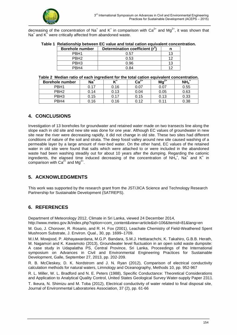
decreasing of the concentration of Na+ and K+ in comparison with Ca2+ and Mg2+, it was shown that Na+ and K+ were critically affected from abandoned waste.
Table 1 Relationship between EC value and total cation equivalent concentration. Borehole number Determination coefficient (r2) n
PBH1 0.57 13 PBH2 0.53 12 PBH3 0.96 13 PBH4 0.84 12
Table 2 Median ratio of each ingredient for the total cation equivalent concentration.
Borehole number Na+ K+ Ca2+ Mg2+ NH4+
PBH1 0.17 0.16 0.07 0.07 0.55 PBH2 0.14 0.13 0.04 0.05 0.63 PBH3 0.15 0.17 0.15 0.13 0.33 PBH4 0.16 0.16 0.12 0.11 0.38
4. CONCLUSIONS
Investigation of 13 boreholes for groundwater and retained water made on two transects line along the slope each in old site and new site was done for one year. Although EC values of groundwater in new site near the river were decreasing rapidly, it did not change in old site. These two sites had different conditions of nature of the soil and strata. The deep fossil valley around new site caused washing of a permeable layer by a large amount of river-bed water. On the other hand, EC values of the retained water in old site were found that salts which were attached to or were included in the abandoned waste had been washing steadily out for about 10 years after the dumping. Regarding the cationic ingredients, the elapsed time induced decreasing of the concentration of NH4
+, Na+ and K+ in comparison with Ca2+ and Mg2+.
5. ACKNOWLEDGMENTS
This work was supported by the research grant from the JST/JICA Science and Technology Research Partnership for Sustainable Development (SATREPS).
6. REFERENCES
Department of Meteorology 2012, Climate in Sri Lanka, viewed 24 December 2014, http://www.meteo.gov.lk/index.php?option=com_content&view=article&id=106&Itemid=81&lang=en
M. Guo, J. Chorover, R. Rosario, and R. H. Fox (2001), Leachate Chemistry of Field-Weathered Spent Mushroom Substrate, J. Environ. Qual., 30, pp. 1699–1709.
M.I.M. Mowjood, P. Abhayawardana, M.G.P. Bandara, S.M.J. Hettiarachchi, K. Takahiro, G.B.B. Herath, M. Nagamori and K. Kawamoto (2013), Groundwater level fluctuation in an open solid waste dumpsite: A case study in Udapalatha PS, Central Province, Sri Lanka, Proceedings of the International symposium on Advances in Civil and Environmental Engineering Practices for Sustainable Development, Galle, September 27, 2013, pp. 202-209.
R. B. McCleskey, D. K. Nordstrom and J. N. Ryan (2012), Comparison of electrical conductivity calculation methods for natural waters, Limnology and Oceanography, Methods 10, pp. 952-967
R. L. Miller, W. L. Bradford and N. E. Peters (1988), Specific Conductance: Theoretical Considerations and Application to Analytical Quality Control, United States Geological Survey Water-supply Paper 2311.
T. Ikeura, N. Shimizu and M. Toba (2012), Electrical conductivity of water related to final disposal site, Journal of Environmental Laboratories Association, 37 (2), pp. 61-66
154
3rd International Symposium on Advances in Civil and Environmental Engineering Practices for Sustainable Development (ACEPS – 2015)
EC values of the retained water in new site for PBH1 and PBH2 continued to rise from 250 mS/m to 1560 mS/m and from 680 mS/m to 1690 mS/m in May 2013 and April 2014, respectively. It was found that salts which were attached to or were included in the abandoned waste had been washing steadily out as of April, 2014.
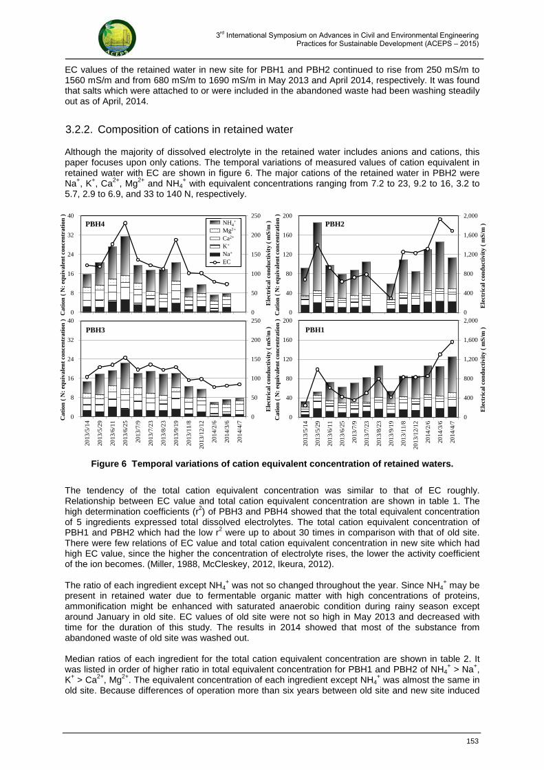
3.2.2. Composition of cations in retained water
Although the majority of dissolved electrolyte in the retained water includes anions and cations, this paper focuses upon only cations. The temporal variations of measured values of cation equivalent in retained water with EC are shown in figure 6. The major cations of the retained water in PBH2 were Na+, K+, Ca2+, Mg2+ and NH4
+ with equivalent concentrations ranging from 7.2 to 23, 9.2 to 16, 3.2 to 5.7, 2.9 to 6.9, and 33 to 140 N, respectively.
Figure 6 Temporal variations of cation equivalent concentration of retained waters.
The tendency of the total cation equivalent concentration was similar to that of EC roughly. Relationship between EC value and total cation equivalent concentration are shown in table 1. The high determination coefficients (r2) of PBH3 and PBH4 showed that the total equivalent concentration of 5 ingredients expressed total dissolved electrolytes. The total cation equivalent concentration of PBH1 and PBH2 which had the low r2 were up to about 30 times in comparison with that of old site. There were few relations of EC value and total cation equivalent concentration in new site which had high EC value, since the higher the concentration of electrolyte rises, the lower the activity coefficient of the ion becomes. (Miller, 1988, McCleskey, 2012, Ikeura, 2012). The ratio of each ingredient except NH4
+ was not so changed throughout the year. Since NH4+ may be
present in retained water due to fermentable organic matter with high concentrations of proteins, ammonification might be enhanced with saturated anaerobic condition during rainy season except around January in old site. EC values of old site were not so high in May 2013 and decreased with time for the duration of this study. The results in 2014 showed that most of the substance from abandoned waste of old site was washed out. Median ratios of each ingredient for the total cation equivalent concentration are shown in table 2. It was listed in order of higher ratio in total equivalent concentration for PBH1 and PBH2 of NH4
+ > Na+, K+ > Ca2+, Mg2+. The equivalent concentration of each ingredient except NH4
+ was almost the same in old site. Because differences of operation more than six years between old site and new site induced
0
400
800
1,200
1,600
2,000
0
40
80
120
160
200
2013
/5/1
4
2013
/5/2
9
2013
/6/1
1
2013
/6/2
5
2013
/7/9
2013
/7/2
3
2013
/8/2
3
2013
/9/1
9
2013
/11/
8
2013
/12/
12
2014
/2/6
2014
/3/6
2014
/4/7
Ele
ctri
cal c
ondu
ctiv
ity
( m
S/m
)
Cat
ion
( N
: eq
uiva
lent
con
cent
rati
on )
PBH2
0
400
800
1,200
1,600
2,000
0
40
80
120
160
200
2013
/5/1
4
2013
/5/2
9
2013
/6/1
1
2013
/6/2
5
2013
/7/9
2013
/7/2
3
2013
/8/2
3
2013
/9/1
9
2013
/11/
8
2013
/12/
12
2014
/2/6
2014
/3/6
2014
/4/7
Ele
ctri
cal c
ondu
ctiv
ity
( m
S/m
)
Cat
ion
( N
: eq
uiva
lent
con
cent
rati
on )
PBH1
0
50
100
150
200
250
0
8
16
24
32
40
2013
/5/1
4
2013
/5/2
9
2013
/6/1
1
2013
/6/2
5
2013
/7/9
2013
/7/2
3
2013
/8/2
3
2013
/9/1
9
2013
/11/
8
2013
/12/
12
2014
/2/6
2014
/3/6
2014
/4/7
Ele
ctri
cal c
ondu
ctiv
ity
( m
S/m
)
Cat
ion
( N
: eq
uiva
lent
con
cent
rati
on )
PBH4 NH4+Mg2+Ca2+K+Na+EC
0
50
100
150
200
250
0
8
16
24
32
40
2013
/5/1
4
2013
/5/2
9
2013
/6/1
1
2013
/6/2
5
2013
/7/9
2013
/7/2
3
2013
/8/2
3
2013
/9/1
9
2013
/11/
8
2013
/12/
12
2014
/2/6
2014
/3/6
2014
/4/7
Ele
ctri
cal c
ondu
ctiv
ity
( m
S/m
)
Cat
ion
( N
: eq
uiva
lent
con
cent
rati
on )
PBH3
NH4+
Mg2+
Ca2+
K+
Na+
EC
153
3rd International Symposium on Advances in Civil and Environmental Engineering Practices for Sustainable Development (ACEPS – 2015)
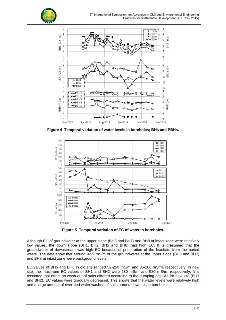
Figure 4 Temporal variation of water levels in boreholes; BHs and PBHs.
Figure 5 Temporal variation of EC of water in boreholes.
Although EC of groundwater at the upper slope (BH3 and BH7) and BH8 at intact zone were relatively low values, the down slope (BH1, BH2, BH5 and BH6) had high EC. It is presumed that the groundwater of downstream was high EC because of penetration of the leachate from the buried waste. The data show that around 9-99 mS/m of the groundwater at the upper slope (BH3 and BH7) and BH8 at intact zone were background levels. EC values of BH5 and BH6 in old site ranged 52-250 mS/m and 85-200 mS/m, respectively. In new site, the maximum EC values of BH1 and BH2 were 530 mS/m and 580 mS/m, respectively. It is assumed that effect on wash-out of salts differed according to the dumping age. As for new site (BH1 and BH2), EC values were gradually decreased. This shows that the water levels were relatively high and a large amount of river-bed water washed of salts around down slope boreholes.
0
100
200
300
400
500
600
Feb-2013 Jul-2013 Dec-2013 May-2014
EC
( m
S/m
)
BH5BH6BH7BH8
0
100
200
300
400
500
600
Feb-2013 Jul-2013 Dec-2013 May-2014
EC
( m
S/m
)
BH1BH2BH3
0
400
800
1200
1600
2000
Feb-2013 Jul-2013 Dec-2013 May-2014
EC
( m
S/m
)
PBH1PBH2PBH3PBH4
3
4
5
6
7
8
0
1
2
3
4
5Nov-2012 Apr-2013 Aug-2013 Jan-2014 Jun-2014 Nov-2014
BH
6 (
m )
BH
5, 7
, 8 (
m )
BH5BH7BH8BH6
7
8
9
10
11
12
0
1
2
3
4
5Nov-2012 Apr-2013 Aug-2013 Jan-2014 Jun-2014 Nov-2014
BH
3 (
m )
BH
1~2
( m
)
BH1BH2BH3
4
5
6
7
8
9
0
1
2
3
4
5Nov-2012 Apr-2013 Aug-2013 Jan-2014 Jun-2014 Nov-2014
PBH
5 (
m )
PBH
1~4
( m
)
PBH1PBH2PBH3PBH4PBH5
152
3rd International Symposium on Advances in Civil and Environmental Engineering Practices for Sustainable Development (ACEPS – 2015)
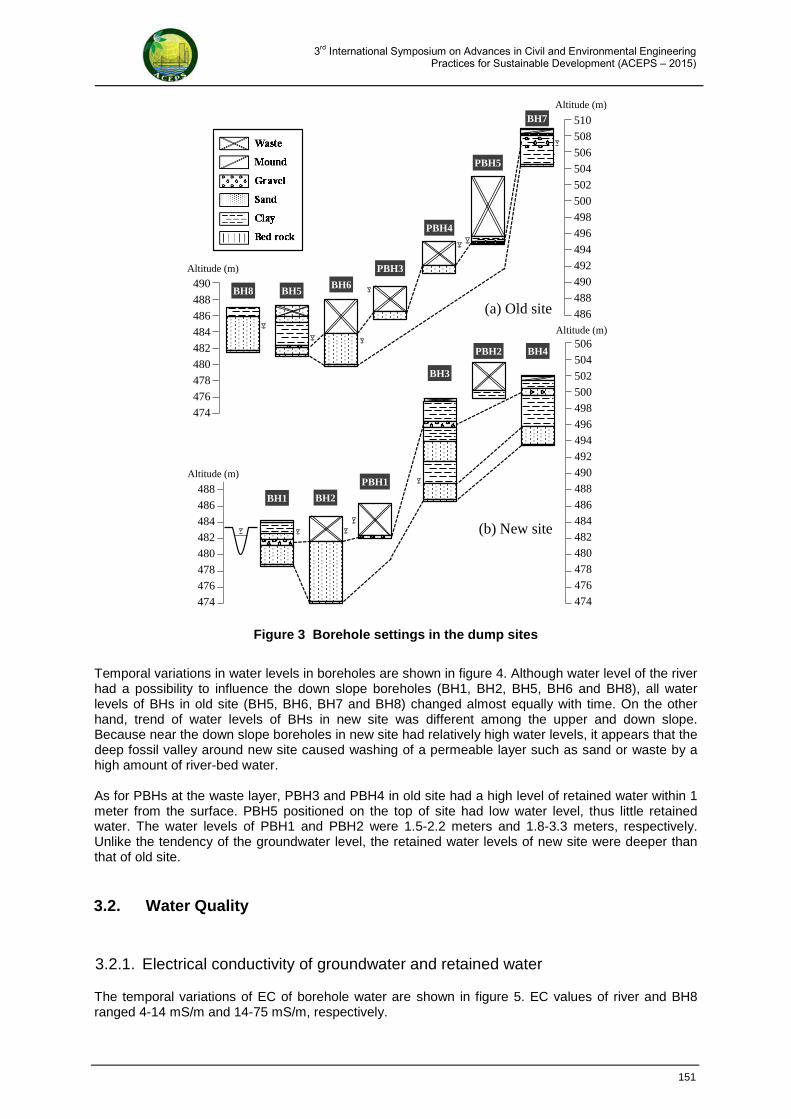
Figure 3 Borehole settings in the dump sites
Temporal variations in water levels in boreholes are shown in figure 4. Although water level of the river had a possibility to influence the down slope boreholes (BH1, BH2, BH5, BH6 and BH8), all water levels of BHs in old site (BH5, BH6, BH7 and BH8) changed almost equally with time. On the other hand, trend of water levels of BHs in new site was different among the upper and down slope. Because near the down slope boreholes in new site had relatively high water levels, it appears that the deep fossil valley around new site caused washing of a permeable layer such as sand or waste by a high amount of river-bed water. As for PBHs at the waste layer, PBH3 and PBH4 in old site had a high level of retained water within 1 meter from the surface. PBH5 positioned on the top of site had low water level, thus little retained water. The water levels of PBH1 and PBH2 were 1.5-2.2 meters and 1.8-3.3 meters, respectively. Unlike the tendency of the groundwater level, the retained water levels of new site were deeper than that of old site.
3.2. Water Quality
3.2.1. Electrical conductivity of groundwater and retained water
The temporal variations of EC of borehole water are shown in figure 5. EC values of river and BH8 ranged 4-14 mS/m and 14-75 mS/m, respectively.
BH8 BH5
PBH3
PBH5
BH7
(a) Old site
PBH4
BH6
510
508
506
504
502
500
498
496
494
492
490
488
486
490
488
486
484
482
480
478
476
474
Altitude (m)
Altitude (m)
BH1 BH2
PBH1
PBH2
BH3
BH4
(b) New site
506
504
502500
498
496494
492
490488
486
484
482
480
478
476
474
488
486
484
482480
478
476474
Altitude (m)
Altitude (m)
151
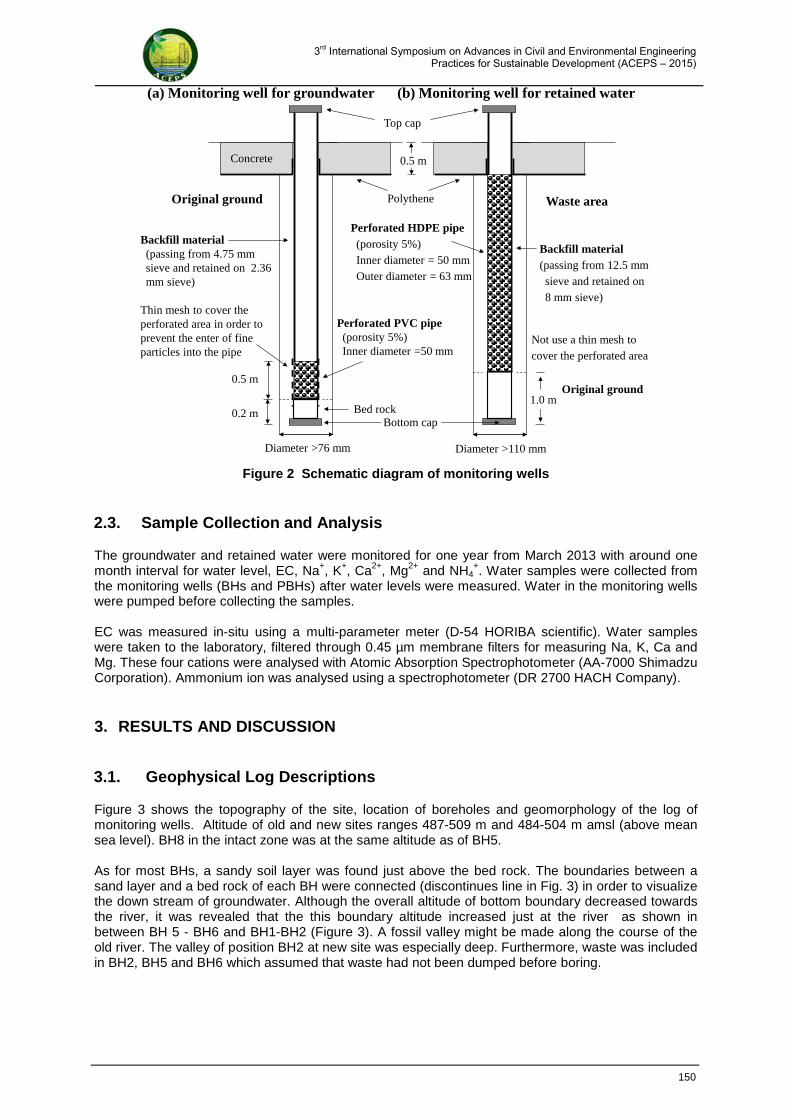
3rd International Symposium on Advances in Civil and Environmental Engineering Practices for Sustainable Development (ACEPS – 2015)
Figure 2 Schematic diagram of monitoring wells
2.3. Sample Collection and Analysis
The groundwater and retained water were monitored for one year from March 2013 with around one month interval for water level, EC, Na+, K+, Ca2+, Mg2+ and NH4
+. Water samples were collected from the monitoring wells (BHs and PBHs) after water levels were measured. Water in the monitoring wells were pumped before collecting the samples. EC was measured in-situ using a multi-parameter meter (D-54 HORIBA scientific). Water samples were taken to the laboratory, filtered through 0.45 µm membrane filters for measuring Na, K, Ca and Mg. These four cations were analysed with Atomic Absorption Spectrophotometer (AA-7000 Shimadzu Corporation). Ammonium ion was analysed using a spectrophotometer (DR 2700 HACH Company).
3. RESULTS AND DISCUSSION
3.1. Geophysical Log Descriptions
Figure 3 shows the topography of the site, location of boreholes and geomorphology of the log of monitoring wells. Altitude of old and new sites ranges 487-509 m and 484-504 m amsl (above mean sea level). BH8 in the intact zone was at the same altitude as of BH5. As for most BHs, a sandy soil layer was found just above the bed rock. The boundaries between a sand layer and a bed rock of each BH were connected (discontinues line in Fig. 3) in order to visualize the down stream of groundwater. Although the overall altitude of bottom boundary decreased towards the river, it was revealed that the this boundary altitude increased just at the river as shown in between BH 5 - BH6 and BH1-BH2 (Figure 3). A fossil valley might be made along the course of the old river. The valley of position BH2 at new site was especially deep. Furthermore, waste was included in BH2, BH5 and BH6 which assumed that waste had not been dumped before boring.
Original ground
Bed rock0.2 m
Polythene
Concrete
Perforated PVC pipe (porosity 5%)Inner diameter =50 mm
Diameter >76 mm
Backfill material(passing from 4.75 mm sieve and retained on 2.36 mm sieve)
0.5 m
Thin mesh to cover the perforated area in order to prevent the enter of fine particles into the pipe
Bottom cap
Top cap
Waste area
Original ground
Perforated HDPE pipe (porosity 5%)Inner diameter = 50 mmOuter diameter = 63 mm
Diameter >110 mm
Backfill material (passing from 12.5 mm sieve and retained on 8 mm sieve)
Not use a thin mesh to cover the perforated area
1.0 m
0.5 m
(a) Monitoring well for groundwater (b) Monitoring well for retained water
150
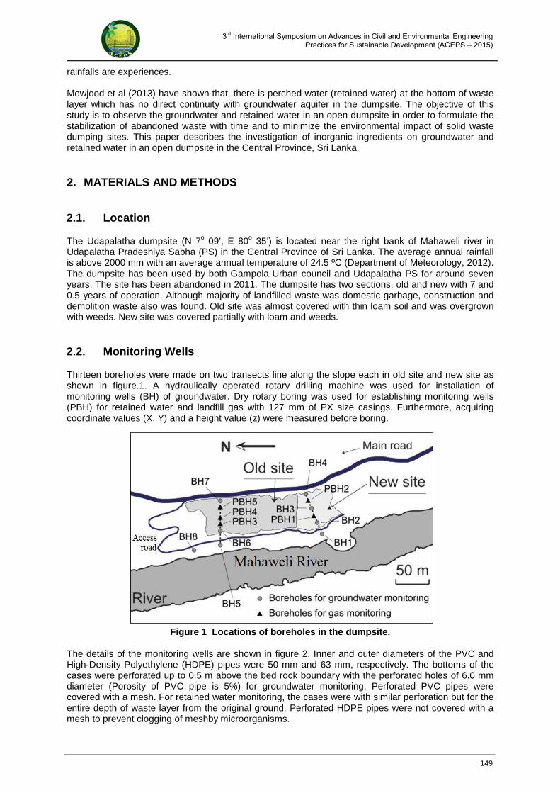
3rd International Symposium on Advances in Civil and Environmental Engineering Practices for Sustainable Development (ACEPS – 2015)
rainfalls are experiences. Mowjood et al (2013) have shown that, there is perched water (retained water) at the bottom of waste layer which has no direct continuity with groundwater aquifer in the dumpsite. The objective of this study is to observe the groundwater and retained water in an open dumpsite in order to formulate the stabilization of abandoned waste with time and to minimize the environmental impact of solid waste dumping sites. This paper describes the investigation of inorganic ingredients on groundwater and retained water in an open dumpsite in the Central Province, Sri Lanka.
2. MATERIALS AND METHODS
2.1. Location
The Udapalatha dumpsite (N 7o 09’, E 80o 35’) is located near the right bank of Mahaweli river in Udapalatha Pradeshiya Sabha (PS) in the Central Province of Sri Lanka. The average annual rainfall is above 2000 mm with an average annual temperature of 24.5 ºC (Department of Meteorology, 2012). The dumpsite has been used by both Gampola Urban council and Udapalatha PS for around seven years. The site has been abandoned in 2011. The dumpsite has two sections, old and new with 7 and 0.5 years of operation. Although majority of landfilled waste was domestic garbage, construction and demolition waste also was found. Old site was almost covered with thin loam soil and was overgrown with weeds. New site was covered partially with loam and weeds.
2.2. Monitoring Wells
Thirteen boreholes were made on two transects line along the slope each in old site and new site as shown in figure.1. A hydraulically operated rotary drilling machine was used for installation of monitoring wells (BH) of groundwater. Dry rotary boring was used for establishing monitoring wells (PBH) for retained water and landfill gas with 127 mm of PX size casings. Furthermore, acquiring coordinate values (X, Y) and a height value (z) were measured before boring.
Figure 1 Locations of boreholes in the dumpsite. The details of the monitoring wells are shown in figure 2. Inner and outer diameters of the PVC and High-Density Polyethylene (HDPE) pipes were 50 mm and 63 mm, respectively. The bottoms of the cases were perforated up to 0.5 m above the bed rock boundary with the perforated holes of 6.0 mm diameter (Porosity of PVC pipe is 5%) for groundwater monitoring. Perforated PVC pipes were covered with a mesh. For retained water monitoring, the cases were with similar perforation but for the entire depth of waste layer from the original ground. Perforated HDPE pipes were not covered with a mesh to prevent clogging of meshby microorganisms.
149
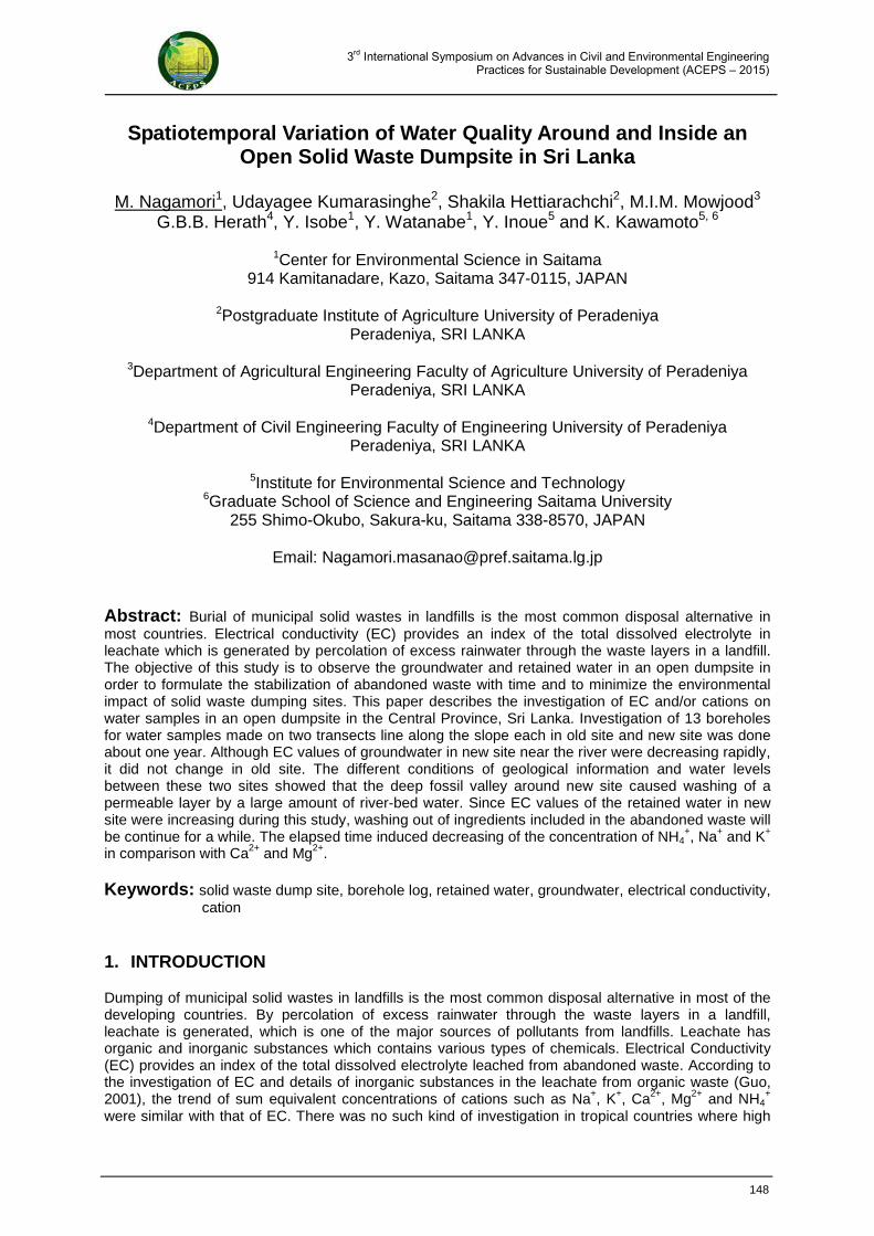
3rd International Symposium on Advances in Civil and Environmental Engineering Practices for Sustainable Development (ACEPS – 2015)
Spatiotemporal Variation of Water Quality Around and Inside an Open Solid Waste Dumpsite in Sri Lanka
M. Nagamori1, Udayagee Kumarasinghe2, Shakila Hettiarachchi2, M.I.M. Mowjood3
G.B.B. Herath4, Y. Isobe1, Y. Watanabe1, Y. Inoue5 and K. Kawamoto5, 6
1Center for Environmental Science in Saitama 914 Kamitanadare, Kazo, Saitama 347-0115, JAPAN
2Postgraduate Institute of Agriculture University of Peradeniya
Peradeniya, SRI LANKA
3Department of Agricultural Engineering Faculty of Agriculture University of Peradeniya Peradeniya, SRI LANKA
4Department of Civil Engineering Faculty of Engineering University of Peradeniya
Peradeniya, SRI LANKA
5Institute for Environmental Science and Technology 6Graduate School of Science and Engineering Saitama University
255 Shimo-Okubo, Sakura-ku, Saitama 338-8570, JAPAN
Email: [email protected]
Abstract: Burial of municipal solid wastes in landfills is the most common disposal alternative in most countries. Electrical conductivity (EC) provides an index of the total dissolved electrolyte in leachate which is generated by percolation of excess rainwater through the waste layers in a landfill. The objective of this study is to observe the groundwater and retained water in an open dumpsite in order to formulate the stabilization of abandoned waste with time and to minimize the environmental impact of solid waste dumping sites. This paper describes the investigation of EC and/or cations on water samples in an open dumpsite in the Central Province, Sri Lanka. Investigation of 13 boreholes for water samples made on two transects line along the slope each in old site and new site was done about one year. Although EC values of groundwater in new site near the river were decreasing rapidly, it did not change in old site. The different conditions of geological information and water levels between these two sites showed that the deep fossil valley around new site caused washing of a permeable layer by a large amount of river-bed water. Since EC values of the retained water in new site were increasing during this study, washing out of ingredients included in the abandoned waste will be continue for a while. The elapsed time induced decreasing of the concentration of NH4
+, Na+ and K+ in comparison with Ca2+ and Mg2+. Keywords: solid waste dump site, borehole log, retained water, groundwater, electrical conductivity,
cation
1. INTRODUCTION
Dumping of municipal solid wastes in landfills is the most common disposal alternative in most of the developing countries. By percolation of excess rainwater through the waste layers in a landfill, leachate is generated, which is one of the major sources of pollutants from landfills. Leachate has organic and inorganic substances which contains various types of chemicals. Electrical Conductivity (EC) provides an index of the total dissolved electrolyte leached from abandoned waste. According to the investigation of EC and details of inorganic substances in the leachate from organic waste (Guo, 2001), the trend of sum equivalent concentrations of cations such as Na+, K+, Ca2+, Mg2+ and NH4
+ were similar with that of EC. There was no such kind of investigation in tropical countries where high
148
3rd International Symposium on Advances in Civil and Environmental Engineering Practices for Sustainable Development (ACEPS – 2015)
5. ACKNOWLEDGMENTS
We appreciate the local resident stakeholders and all interview respondents for their kind cooperation to our survey.
6. REFERENCES
Bausch J.C., Bojórquez-Tapia L., Eakin H. (2014). Agro-environmental sustainability assessment using multicriteria decision analysis and system analysis. Sustain. Sci., 9(3), 303-319. Hara Y., Hiramatsu A., Honda R., Sekiyama M., Matsuda H. (2010) Mixed land-use planning on the periphery of large Asian cities: the case of Nonthaburi Province, Thailand. Sustain. Sci. 5(2), 237-248. Hiramatsu A., Hara Y., Sekiyama M., Honda R. (2009) Municipal solid waste flow and waste generation characteristics in an urban-rural fringe area in Thailand. Waste Management Res. 27(10), 951-960. Hirayama N., Nakamura M., Ide S. (2011) Proposal of a Tool for Evaluating People’s Values of Lake Biwa. Lakes & Reservoirs: Research and Management 16(3), 205-209. Hirayama N., Nakamura M., Ide S., (2005) Proposal of a supportive tool for Consensus Building on advanced tertiary treatment systems in Shiga, Environ. Sys. Res.. 33, 431-440. (in Japanese) Honda R., Hara Y., Sekiyama M., Hiramatsu A. (2010) Impacts of housing development on nutrients flow along canals in a peri-urban area of Bangkok, Thailand. Water Sci. Technol. 61(4), 1073-1080. Hsu, A., J. Emerson, M. Levy, A. de Sherbinin, L. Johnson, O. Malik, J. Schwartz, M. Jaiteh. (2014). The 2014 Environmental Performance Index. New Haven, CT: Yale Center for Environmental Law & Policy. Available: www.epi.yale.edu. Kawakami T., Weragoda S.K., Attanayake M.A.M.S.L., Sakamoto M., Tafu M., Honoki H., Serikawa Y. (2011) Fish die-off and water quality in Kandy Lake, a world heritage site in Sri Lanka. J. Ecotechnol. Res., 16(2), 39-45.
147
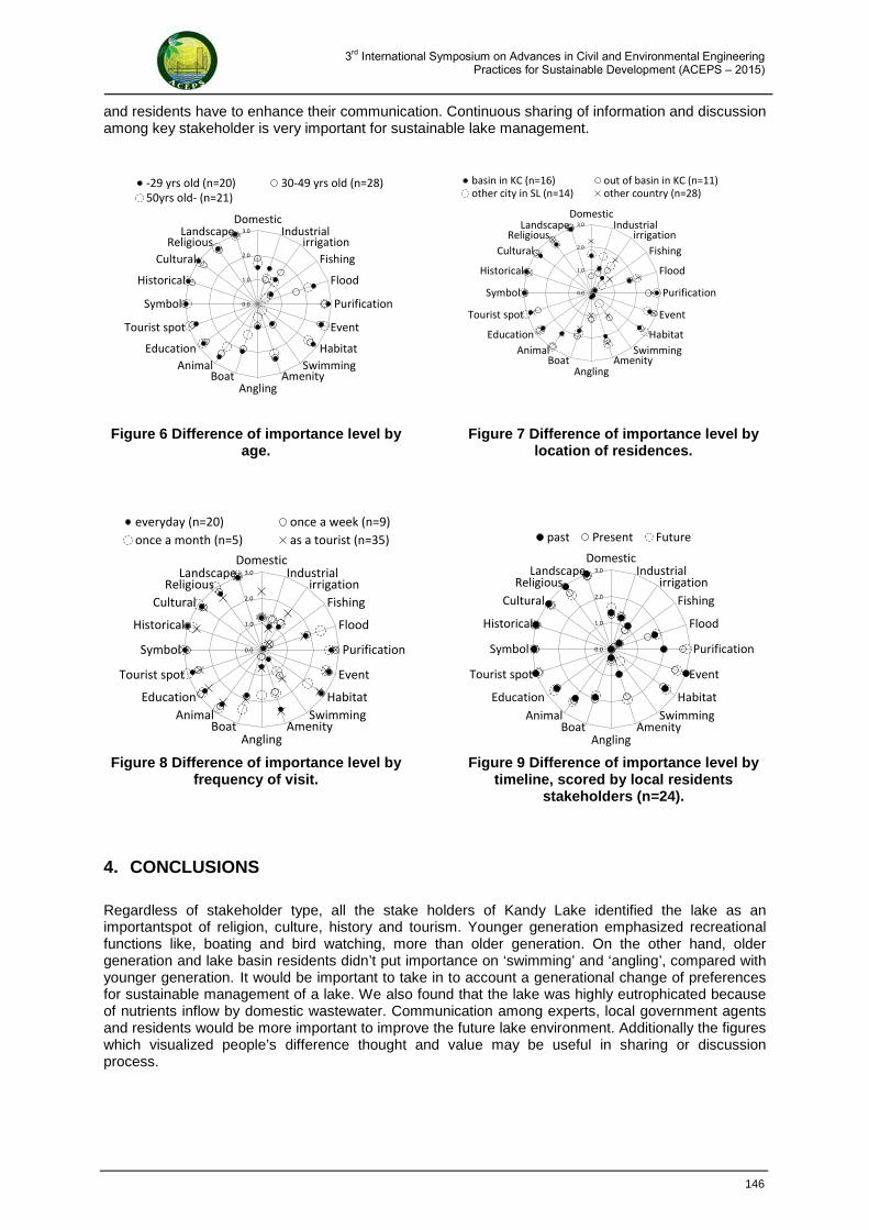
3rd International Symposium on Advances in Civil and Environmental Engineering Practices for Sustainable Development (ACEPS – 2015)
and residents have to enhance their communication. Continuous sharing of information and discussion among key stakeholder is very important for sustainable lake management.
Figure 6 Difference of importance level by
age. Figure 7 Difference of importance level by
location of residences.
Figure 8 Difference of importance level by frequency of visit.
Figure 9 Difference of importance level by timeline, scored by local residents
stakeholders (n=24).
4. CONCLUSIONS
Regardless of stakeholder type, all the stake holders of Kandy Lake identified the lake as an importantspot of religion, culture, history and tourism. Younger generation emphasized recreational functions like, boating and bird watching, more than older generation. On the other hand, older generation and lake basin residents didn’t put importance on ‘swimming’ and ‘angling’, compared with younger generation. It would be important to take in to account a generational change of preferences for sustainable management of a lake. We also found that the lake was highly eutrophicated because of nutrients inflow by domestic wastewater. Communication among experts, local government agents and residents would be more important to improve the future lake environment. Additionally the figures which visualized people’s difference thought and value may be useful in sharing or discussion process.
0.0
1.0
2.0
3.0Domestic
Industrialirrigation
Fishing
Flood
Purification
Event
HabitatSwimming
AmenityAngling
BoatAnimal
Education
Tourist spot
Symbol
Historical
CulturalReligious
Landscape
-29 yrs old (n=20) 30-49 yrs old (n=28)50yrs old- (n=21)
0.0
1.0
2.0
3.0Domestic
Industrialirrigation
Fishing
Flood
Purification
Event
HabitatSwimming
AmenityAngling
BoatAnimal
Education
Tourist spot
Symbol
Historical
CulturalReligious
Landscape
basin in KC (n=16) out of basin in KC (n=11)other city in SL (n=14) other country (n=28)
0.0
1.0
2.0
3.0
DomesticIndustrial
irrigationFishing
Flood
Purification
Event
HabitatSwimming
AmenityAngling
BoatAnimal
Education
Tourist spot
Symbol
Historical
CulturalReligious
Landscape
past Present Future
0.0
1.0
2.0
3.0Domestic
Industrialirrigation
Fishing
Flood
Purification
Event
HabitatSwimming
AmenityAngling
BoatAnimal
Education
Tourist spot
Symbol
Historical
CulturalReligious
Landscape
everyday (n=20) once a week (n=9)once a month (n=5) as a tourist (n=35)
146
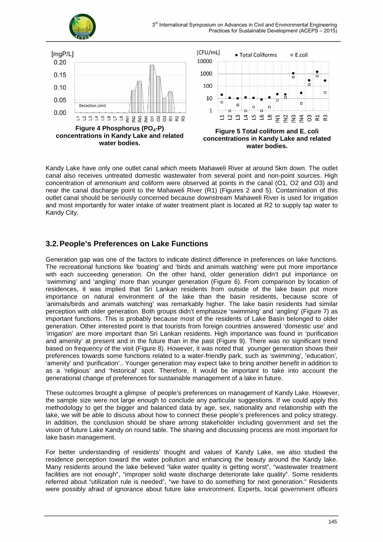
3rd International Symposium on Advances in Civil and Environmental Engineering Practices for Sustainable Development (ACEPS – 2015)
Kandy Lake have only one outlet canal which meets Mahaweli River at around 5km down. The outlet canal also receives untreated domestic wastewater from several point and non-point sources. High concentration of ammonium and coliform were observed at points in the canal (O1, O2 and O3) and near the canal discharge point to the Mahaweli River (R1) (Figures 2 and 5). Contamination of this outlet canal should be seriously concerned because downstream Mahaweli River is used for irrigation and most importantly for water intake of water treatment plant is located at R2 to supply tap water to Kandy City.
3.2. People’s Preferences on Lake Functions
Generation gap was one of the factors to indicate distinct difference in preferences on lake functions. The recreational functions like ‘boating’ and ‘birds and animals watching’ were put more importance with each succeeding generation. On the other hand, older generation didn’t put importance on ‘swimming’ and ‘angling’ more than younger generation (Figure 6). From comparison by location of residences, it was implied that Sri Lankan residents from outside of the lake basin put more importance on natural environment of the lake than the basin residents, because score of ‘animals/birds and animals watching’ was remarkably higher. The lake basin residents had similar perception with older generation. Both groups didn’t emphasize ‘swimming’ and ‘angling’ (Figure 7) as important functions. This is probably because most of the residents of Lake Basin belonged to older generation. Other interested point is that tourists from foreign countries answered ‘domestic use’ and ‘irrigation’ are more important than Sri Lankan residents. High importance was found in ‘purification and amenity’ at present and in the future than in the past (Figure 9). There was no significant trend based on frequency of the visit (Figure 8). However, it was noted that younger generation shows their preferences towards some functions related to a water-friendly park, such as ‘swimming’, ‘education’, ‘amenity’ and ‘purification’.. Younger generation may expect lake to bring another benefit in addition to as a ‘religious’ and ‘historical’ spot. Therefore, It would be important to take into account the generational change of preferences for sustainable management of a lake in future. These outcomes brought a glimpse of people’s preferences on management of Kandy Lake. However, the sample size were not large enough to conclude any particular suggestions. If we could apply this methodology to get the bigger and balanced data by age, sex, nationality and relationship with the lake, we will be able to discuss about how to connect these people’s preferences and policy strategy. In addition, the conclusion should be share among stakeholder including government and set the vision of future Lake Kandy on round table. The sharing and discussing process are most important for lake basin management. For better understanding of residents’ thought and values of Kandy Lake, we also studied the residence perception toward the water pollution and enhancing the beauty around the Kandy lake. Many residents around the lake believed “lake water quality is getting worst”, “wastewater treatment facilities are not enough”, “improper solid waste discharge deteriorate lake quality”. Some residents referred about “utilization rule is needed”, “we have to do something for next generation.” Residents were possibly afraid of ignorance about future lake environment. Experts, local government officers
Figure 4 Phosphorus (PO4-P) concentrations in Kandy Lake and related
water bodies.
Figure 5 Total coliform and E. coli concentrations in Kandy Lake and related
water bodies.
145
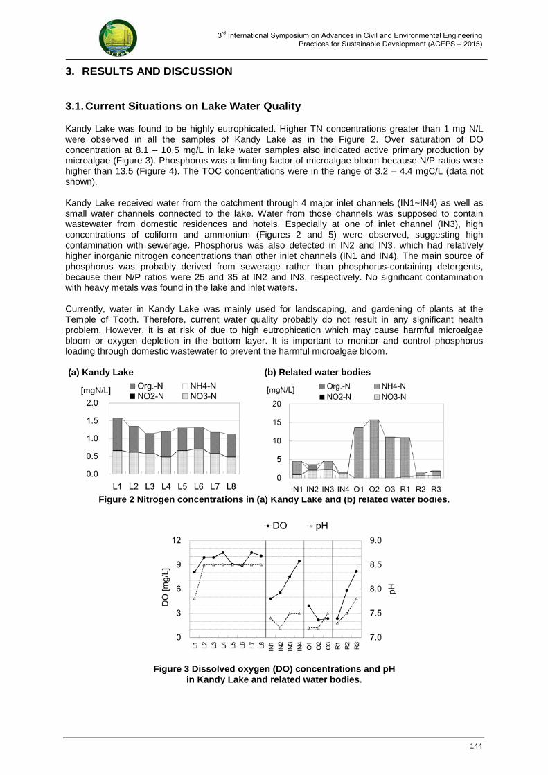
3rd International Symposium on Advances in Civil and Environmental Engineering Practices for Sustainable Development (ACEPS – 2015)
3. RESULTS AND DISCUSSION
3.1. Current Situations on Lake Water Quality
Kandy Lake was found to be highly eutrophicated. Higher TN concentrations greater than 1 mg N/L were observed in all the samples of Kandy Lake as in the Figure 2. Over saturation of DO concentration at 8.1 – 10.5 mg/L in lake water samples also indicated active primary production by microalgae (Figure 3). Phosphorus was a limiting factor of microalgae bloom because N/P ratios were higher than 13.5 (Figure 4). The TOC concentrations were in the range of 3.2 – 4.4 mgC/L (data not shown). Kandy Lake received water from the catchment through 4 major inlet channels (IN1~IN4) as well as small water channels connected to the lake. Water from those channels was supposed to contain wastewater from domestic residences and hotels. Especially at one of inlet channel (IN3), high concentrations of coliform and ammonium (Figures 2 and 5) were observed, suggesting high contamination with sewerage. Phosphorus was also detected in IN2 and IN3, which had relatively higher inorganic nitrogen concentrations than other inlet channels (IN1 and IN4). The main source of phosphorus was probably derived from sewerage rather than phosphorus-containing detergents, because their N/P ratios were 25 and 35 at IN2 and IN3, respectively. No significant contamination with heavy metals was found in the lake and inlet waters. Currently, water in Kandy Lake was mainly used for landscaping, and gardening of plants at the Temple of Tooth. Therefore, current water quality probably do not result in any significant health problem. However, it is at risk of due to high eutrophication which may cause harmful microalgae bloom or oxygen depletion in the bottom layer. It is important to monitor and control phosphorus loading through domestic wastewater to prevent the harmful microalgae bloom. (a) Kandy Lake (b) Related water bodies
Figure 2 Nitrogen concentrations in (a) Kandy Lake and (b) related water bodies.
Figure 3 Dissolved oxygen (DO) concentrations and pH in Kandy Lake and related water bodies.
144
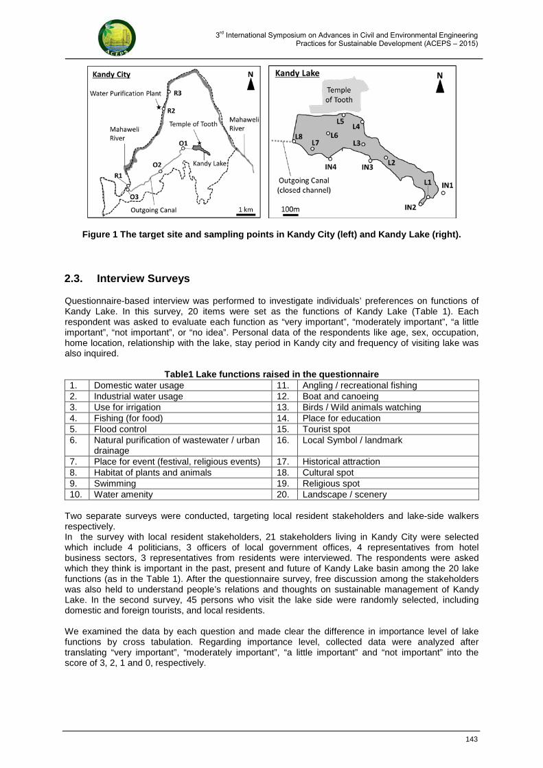
3rd International Symposium on Advances in Civil and Environmental Engineering Practices for Sustainable Development (ACEPS – 2015)
Figure 1 The target site and sampling points in Kandy City (left) and Kandy Lake (right).
2.3. Interview Surveys
Questionnaire-based interview was performed to investigate individuals’ preferences on functions of Kandy Lake. In this survey, 20 items were set as the functions of Kandy Lake (Table 1). Each respondent was asked to evaluate each function as “very important”, “moderately important”, “a little important”, “not important”, or “no idea”. Personal data of the respondents like age, sex, occupation, home location, relationship with the lake, stay period in Kandy city and frequency of visiting lake was also inquired.
Table1 Lake functions raised in the questionnaire 1. Domestic water usage 11. Angling / recreational fishing 2. Industrial water usage 12. Boat and canoeing 3. Use for irrigation 13. Birds / Wild animals watching 4. Fishing (for food) 14. Place for education 5. Flood control 15. Tourist spot 6. Natural purification of wastewater / urban
drainage 16. Local Symbol / landmark
7. Place for event (festival, religious events) 17. Historical attraction 8. Habitat of plants and animals 18. Cultural spot 9. Swimming 19. Religious spot 10. Water amenity 20. Landscape / scenery
Two separate surveys were conducted, targeting local resident stakeholders and lake-side walkers respectively. In the survey with local resident stakeholders, 21 stakeholders living in Kandy City were selected which include 4 politicians, 3 officers of local government offices, 4 representatives from hotel business sectors, 3 representatives from residents were interviewed. The respondents were asked which they think is important in the past, present and future of Kandy Lake basin among the 20 lake functions (as in the Table 1). After the questionnaire survey, free discussion among the stakeholders was also held to understand people’s relations and thoughts on sustainable management of Kandy Lake. In the second survey, 45 persons who visit the lake side were randomly selected, including domestic and foreign tourists, and local residents. We examined the data by each question and made clear the difference in importance level of lake functions by cross tabulation. Regarding importance level, collected data were analyzed after translating “very important”, “moderately important”, “a little important” and “not important” into the score of 3, 2, 1 and 0, respectively.
143
3rd International Symposium on Advances in Civil and Environmental Engineering Practices for Sustainable Development (ACEPS – 2015)
evaluators or stakeholders. Therefore, in developing such polices for a sustainable society, it is important to clarify people’s preferences to decide resources allocation for implementation. Kandy Lake is an artificial lake built in 1807 besides the Temple of the Sacred Tooth Relic, in Kandy City, a UNESCO world heritage site and one of the famous tourist spots in Sri Lanka.. However, due to the rapid urban development and increase of tourists, severe pollution of the lake is recently concerned. In 2009, a massive die-off of fish was reported in Kandy Lake (Kawakami et al., 2011). However, because of the symbolic nature of the lake, opinions of various stakeholders, including local residents and tourists, should be carefully reflected in making policies for sustainable management of Kandy Lake. Their thought and preferences on the lake management may vary dependent on of the nature of stakeholders;local residents or tourists, age, education level, occupation, etc. To measure people’s preferences, Hirayama et al. (2011) reported that Analytic Hierarchy Process (AHP) was useful to clarify relative importance levels of lake functions by residents in Biwa Lake basin, Japan. Moreover, it was clarified that willingness-to-pay (WTP) of each policy could be calculated as the product of the WTP including people’s value for lake and that the weight of the lake function could be evaluated by residents and government officers with AHP and contingent valuation method (Hirayama et al, 2005). In this study, we investigated people’s preference on lake functions to reveal factors which affect deference in importance level among people. That would be useful for sustainable management of Kandy Lake with good consensus of people and for development of a better methodology of sustainability assessment on water environment.
2. MATERIALS AND METHODS
2.1. Target Area
Kandy Lake and surrounding area were selected as the target area (Figure 1). Kandy Lake is an artificial lake built in 1807 besides the Temple of Tooth in Kandy City, Sri Lanka. Its surface area is 14.7 ha and perimeter is 3.3 km. Kandy City is located in a tropical rainforest area. Average annual precipitation is 1,840 mm. Kandy City had 125,400 of population and 4,600 persons/km2 of density in 2011. Sewage treatment system in Kandy was currently under planning and not in service at the moment.
2.2. Water Quality
To investigate the current conditions of water quality in the target area, water samples were collected at total 18 sites: 8 locations in Kandy Lake (L1-L8), 4 inlet water channels (IN1-4), 3 locations in outlet canal (O1-3) and 3 locations in Mahaweli River, which receives water from the outlet canal (R1-3) (Figure 1). Samples were kept in a cool condition until analyzed, except during travel from Kandy to Tokyo for about 16 hours. Total organic carbon (TOC), dissolved organic carbon (DOC), total nitrogen (TN) and dissolved nitrogen (DN) concentrations were analyzed by a TOC analyzer (TOC-V, Shimadzu, Japan). The major cations and anions were analyzed by an ion chromatography system (LC-20A Series, Shimadzu, Japan). These analyses were conducted within 6 days after sampling, the minimum period of shipping from Kandy to Kanazawa, Japan, where samples were analyzed for chemical parameters. Heavy metals were analyzed by an ICP-MS (Agilent 7700, USA). Fourteen samples were selected for total coliform and E. coli analyses by colony counting on the very day of sampling in Sri Lanka, by colony counting on Chromocult Coliform Agar ES (Merck Millipore, USA).
142
3rd International Symposium on Advances in Civil and Environmental Engineering Practices for Sustainable Development (ACEPS – 2015)
A Pilot Study of Water Quality and People’s Importance Level towards Sustainable Management of Kandy Lake Basin, Sri Lanka
Naoko HIRAYAMA1, Ryo HONDA2, G. Tushara CHAMINDA3,
Sujithra K. WERAGODA4, N.I. WICKREMASINGHE4, Gayan AMARASOORIYA5, Yuta TERAOKA6 and Tomonori KAWAKAMI7
1Department of Environmental Policy and Planning, School of Environmental Science,
The University of Shiga Prefecture, Hikone, Japan
2Research Center for Sustainable Energy and Technology, Institute of Science and Engineering, Kanazawa University, Kanazawa, Japan
3Department of Civil and Environmental Engineering, Faculty of Engineering,
University of Ruhuna, Galle, Sri Lanka
4National Water Supply & Drainage Board, Peradeniya, Sri Lanka
5Post Graduate Institute of Science, University of Peradeniya, Peradeniya, Sri Lanka
6Division of Environmental Design, Graduate School of Natural Science and Technology, Kanazawa University, Kanazawa, Japan
7Faculty of Engineering, Toyama Prefectural University, Imizu, Japan
E-mail: [email protected]
Abstract: This study aimed to clarify the factors affecting people’s preferences for sustainable management of Kandy lake basin, Sri Lanka. We conducted water sampling surveys to clarify the current situation on water quality of the lake and related water bodies, and an interview survey to investigate preferences of local people and tourists on functions of Kandy Lake. As the result, the lake was highly eutrophicated because of nutrients inflow by domestic wastewater, as local residents had recognized. Regardless of respondents’ property, high importance levels were observed in functions as a spot of religion, culture, history and tourism. Younger generation emphasized recreational functions like boating and bird watching, more than older generation. It would be important to watch a generational change of preferences for sustainable management of a lake. Communication among residents, scientist and local government and would be more important to improve the future lake environment. Keywords: sustainability assessment, decision making, water resources management, ecotourism, lake basin development, knowledge sharing process
1. INTRODUCTION
Urbanization sometimes drastically changes materials flow and its balance in a certain area even within a short period (Hara et al., 2010). Such rapid urbanization often results in severe environmental deterioration (Hiramatsu et al., 2009; Honda et al., 2010) because countermeasures, which need to wait for policy-makers’ decision, cannot catch up with the change. Sustainability assessment is one of the important key tools to develop and evaluate policies for a sustainable society. Various indicators have been developed to evaluate sustainability of environment (Hsu et al, 2014; Bausch et al., 2014). Though a number of parameters are to be evaluated in assessment of sustainability from a wide range of aspects like sanitation, ecosystem, etc., many of the indicators developed so far attempt to integrate each parameter by giving a certain weighing formula, which is often decided by experts or scientists including developers of the indicator. However, importance on each aspect often varies dependent on
141

3rd International Symposium on Advances in Civil and Environmental Engineering Practices for Sustainable Development (ACEPS – 2015)
Wakjira M, Berecha G &Bulti B. 2005. Allelopathic effects of Partheniumhysterophorus extracts on seed germination and seedling growth of lettuce. Tropical Science 45 (4): 159-162
140
3rd International Symposium on Advances in Civil and Environmental Engineering Practices for Sustainable Development (ACEPS – 2015)
compatible with leaf leachates of M. micrantha reduced the root and shoot elongation of Oryza sativa and Triticum aestivum etc. (Baral et al.,2011).
5 CONCLUSION
The results of the present study showed that germination of Bidens pilosa seeds was affected by root extracts of both invasive plants. Conversely, target species growth and development only inhibit by M. micrantha aqueous extracts while C. odorata extracts were not influenced for the growth process. It seems that mechanisms of adaptation to alleopathy in both species are not the same and Chromolaena odorata is less allelopathic than to Mikania micrantha in case of Bidens pilosa.
6 ACKNOWLEDGEMENT
This study was financially supported by the project transformation of University of Ruhuna to international status (RU/DVC/PRO138). The authors thank Mr. V. Nandadasa and Ms. D.A.M. NimalShanthi for their support extended in experimental setup preparation and analysis.
7 REFERENCES
Ambika, S.R. 2002. Allelopathic plants. Chromolaenaodorata(L) King and Robinson. Allelopathy Journal. 9(1): 35-41. Baldwin I .T. 2003. At last, evidence of weapons of mass destruction. Science STKE 203: pe42. Baral,B and maharjan,B.L.2011.Antagonistic characteristics and photochemical screening of invasive alien species of Nepal Himalaya.international pharmaceutical & biological archives 2(5):1444-1450. Callaway RM and Aschehoug ET. 2000. Invasive plants versus their new and old neighbors: a mechanism for exotic invasion. Science 290: 521-523. Deng, X., H. Feng, W.H. Ye, and Q. Yang. 2003. A study on the control of exotic weed Mikaniamicrantha by using parasitic Cuscutacampestris. J. Tropical Subtropical Bot. 11: 117-122 Hills, L.A. and Ostermeyer, N. 2000. Siam weed or Christmas bush: (Chromolaena ordorata). Agnote-Northern-Territory-of-Australia. (536): 2. Lowe, S., Browne, M., Boudjelas, S. & De poorter, M. 2000. 100 of the world's worst invasive alien species: a selection from the global invasive species database, Invasive Species Specialist Group Auckland, New Zealand. McEwan, R.W., Arthur-Paratley L.G., Rieske L.K. and Arthur M.A. 2010. A multi-assay comparison of seed germination inhibition by Loniceramaackii and co-occurring native shrubs. Flora 205: 475-483. Mgidia, T.N., Le Maitre, D.C., Schonegevela, L.,Nel, J.L., Rouget, M., and Richardson, D.M.2007 Allien plant invasions-incorporating emerging invaders in regional prioritization: a pragmatic approach for Southern Africa. Journal of Environmental Management 84, 173–187 Oliveira, S.C.C. and Campos, M.L.2006. Allelopathic effects of Solanumpalinacanthum leaves on germination and seedling growth of Sesamumindicum. Allelopathy Journal 18: 331-337. Reigosa, M.J., Sanchez-Moreiras, A. and Gonzalez, L. (1999). Ecophysiological approach in allelopathy. Critical Reviews in Plant Sciences 18: 577-608.
Rice, E.L. (1984). Allelopathy. Academic Press, Orlando, Florida.
Roberts K.J. and Anderson R.C. 2001. Effect of garlic mustard [Alliariapetiolata (Beib. Cavara& Grande)] extracts on plants and arbuscularmycorrhizal (AM) fungi. Am. Midl. Nat. 146: 146 –152. Roy, J. 1990. In search of the characteristics of plant invaders. / In: Di Castri, F., Hansen, A. J. and Debussche, M. (eds), Biological invasions in Europe and the Mediterranean basin. Kluwer Academic Publishers, pp. 333/352. Ruprecht, E., Donath, T.W., Otte, A. and Eckstein, L.R. (2008). Chemical effects of a dominant grass on seed germination of four familial pairs of dry grassland species. Seed Science Research 18: 239-248 Skulman B.W., Mattice J.D., Cain M.D. and Gbur E.E. 2004.Evidence for allelopathic interference of Japanese honeysuckle (Lonicera japonica) to loblolly and shortleaf pine regeneration. Weed Sci. 52: 433 –439. Vitousek PM, D’Antonio CM, Loope LL, Rejma´nek M, Westbrooks R (1997) Introduecd species: a significant component of human-caused global change. N Z J Ecol 21:1–16
139
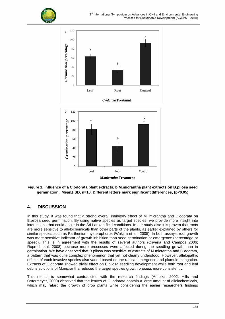
3rd International Symposium on Advances in Civil and Environmental Engineering Practices for Sustainable Development (ACEPS – 2015)
Figure 1. Influence of a C.odorata plant extracts, b M.micrantha plant extracts on B.pilosa seed
germination, Mean± SD, n=10. Different letters mark significant differences, (p<0.05)
4. DISCUSSION
In this study, it was found that a strong overall inhibitory effect of M. micrantha and C.odorata on B.pilosa seed germination. By using native species as target species, we provide more insight into interactions that could occur in the Sri Lankan field conditions. In our study also it is proven that roots are more sensitive to allelochemicals than other parts of the plants, as earlier explained by others for similar species such as Parthenium hysterophorus (Wakjira et al., 2005). In both assays, root growth was more sensitive indicator of growth inhibition than seed germination or emergence (percentage or speed). This is in agreement with the results of several authors (Oliveira and Campos 2006; Ruprechtetal. 2008) because more processes were affected during the seedling growth than in germination. We have observed that B.pilosa was sensitive to extracts of M.micrantha and C.odorata, a pattern that was quite complex phenomenon that yet not clearly understood. However, allelopathic effects of each invasive species also varied based on the radical emergence and plumule elongation. Extracts of C.odorata showed trivial effect on B.pilosa seedling development while both root and leaf debris solutions of M.micrantha reduced the target species growth process more consistently.
This results is somewhat contradicted with the research findings (Ambika, 2002; Hills and Ostermeyer, 2000) observed that the leaves of C. odorata contain a large amount of allelochemicals, which may retard the growth of crop plants while considering the earlier researchers findings
a
b
c
0
20
40
60
80
100
120
Leaf Root Control
Ger
min
ati
on
per
cen
tage
C.odorata Treatment
a
a
b
a
0
20
40
60
80
100
120
Leaf Root Control
Ger
min
atio
n p
erce
nta
ge
M.micrntha Treatment
b
138
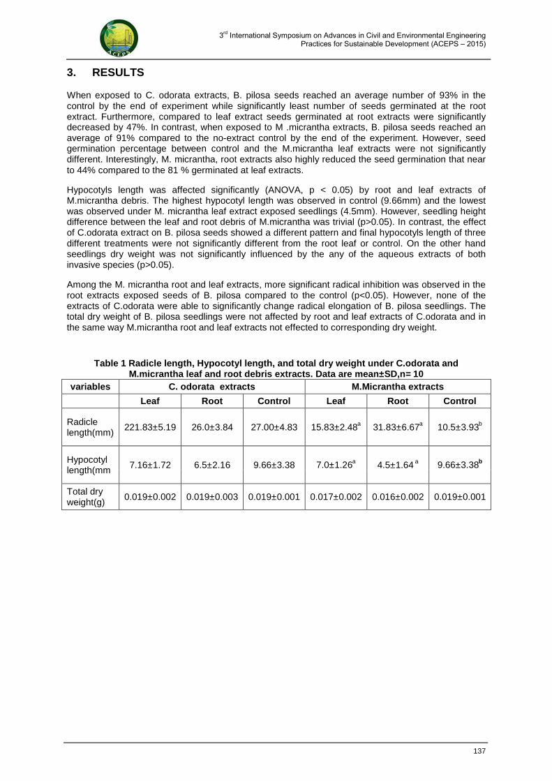
3rd International Symposium on Advances in Civil and Environmental Engineering Practices for Sustainable Development (ACEPS – 2015)
3. RESULTS
When exposed to C. odorata extracts, B. pilosa seeds reached an average number of 93% in the control by the end of experiment while significantly least number of seeds germinated at the root extract. Furthermore, compared to leaf extract seeds germinated at root extracts were significantly decreased by 47%. In contrast, when exposed to M .micrantha extracts, B. pilosa seeds reached an average of 91% compared to the no-extract control by the end of the experiment. However, seed germination percentage between control and the M.micrantha leaf extracts were not significantly different. Interestingly, M. micrantha, root extracts also highly reduced the seed germination that near to 44% compared to the 81 % germinated at leaf extracts.
Hypocotyls length was affected significantly (ANOVA, p < 0.05) by root and leaf extracts of M.micrantha debris. The highest hypocotyl length was observed in control (9.66mm) and the lowest was observed under M. micrantha leaf extract exposed seedlings (4.5mm). However, seedling height difference between the leaf and root debris of M.micrantha was trivial (p>0.05). In contrast, the effect of C.odorata extract on B. pilosa seeds showed a different pattern and final hypocotyls length of three different treatments were not significantly different from the root leaf or control. On the other hand seedlings dry weight was not significantly influenced by the any of the aqueous extracts of both invasive species (p>0.05).
Among the M. micrantha root and leaf extracts, more significant radical inhibition was observed in the root extracts exposed seeds of B. pilosa compared to the control (p<0.05). However, none of the extracts of C.odorata were able to significantly change radical elongation of B. pilosa seedlings. The total dry weight of B. pilosa seedlings were not affected by root and leaf extracts of C.odorata and in the same way M.micrantha root and leaf extracts not effected to corresponding dry weight.
Table 1 Radicle length, Hypocotyl length, and total dry weight under C.odorata and M.micrantha leaf and root debris extracts. Data are mean±SD,n= 10
variables C. odorata extracts M.Micrantha extracts
Leaf Root Control Leaf Root Control
Radicle length(mm)
221.83±5.19 26.0±3.84 27.00±4.83 15.83±2.48a 31.83±6.67a 10.5±3.93b
Hypocotyl length(mm 7.16±1.72 6.5±2.16 9.66±3.38 7.0±1.26a 4.5±1.64 a 9.66±3.38b
Total dry weight(g)
0.019±0.002 0.019±0.003 0.019±0.001 0.017±0.002 0.016±0.002 0.019±0.001
137
3rd International Symposium on Advances in Civil and Environmental Engineering Practices for Sustainable Development (ACEPS – 2015)
these Asteraceae family plant allelochmicals interactions on the growth and plant physiology has been less. In this study we especially incorporated both root and leaf for compare strength of separate sources that valuable for evaluation. Moreover, root mediated allelopathy is one of the neglected area in invasive plant studies (Roberts and Anderson 2001; Skulman et al. 2004). We hypothesized that the presence of leaf and root extracts of C.odorata and M.micrantha would reduce the germination and early seedling development of B.pilosa. The purpose of this experiment was to examine the effect of leaf and root litter extracts on percent germination and seedling growth of B.pilosa specifically focusing allelopathic activity.
2. MATERIALS AND METHODS
2.1 Plant Material
Decomposed leaves and roots of respective two species were collected in nearby heavily infested site within Faculty of Engineering, University of Ruhuna, located in Galle (6o4, 4.72" N, 80o11, 11.5" E) during February-March 2014. After collection of dead leaf and root they were dried at 40oC for 72 hrs and ground manually using mortar and pestle at room temperature (25-26oC). 50g of ground root and leaf matter was dissolved in 500ml distilled water for prepare separate solutions from two species. The extract was left for incubation about 24 hrs and filtered through 2 layers of filter paper (Whatman No.1) and stored in dark conical flasks and then stored in a refrigerator until use.
2.2 Collection of Bidens pilosa Seeds
Healthy uniform seeds of (Bidens pilosa L., family: Asteraceae) was collected from the same site above mentioned. The seeds were soaked in distilled water for one hour. Then the seeds were surface sterilized with 1% H2O2 solution for 5 minutes, and rinsed with double-distilled water several times for complete removal of the sterilant. The effects of the extracts on the germination and seedling growth of B. pilosa was tested by placing 10 seeds in Petri dishes.(6 replications) containing 2 layers of Whatman No.1 filter paper saturated with the extracts (5 ml). A separate control series was also set up using only distilled water. The total numbers of 36 petri dishes were utilized for two experiment and moisture in the petri-dishes was maintained by adding about 2 ml of extract/distilled water (control) as and when required. Total number of seeds germinated after 1 day were counted both in Petri-dishes and compared with the control respectively up to every day for 10 days. Root and shoot length (average of 10 plants) and dry weight (of 10 plants) were taken and compared with the control. The lengths of radicle and hypocotyl of seedlings were measured on a single day when its seeds had reached the maximal germination rate in separate treatments i.e., on day 8 for C.odorata and extracts, and 7 day for M. micrantha extracts exposed seedlings. Corresponding Germination percentage was calculated using below given formula. Germination percentage= Number of germinated seeds/Total number of seeds×100
2.2 Statistical Analysis
The data were subjected to homogeneity (Levene) tests. When this assumption was met, one factor analysis of variance (ANOVA) was performed for all corresponding variables: root dry weight, shoot dry weight, root to shoot ratio etc, for one fixed factor (aqueous extract). The raw data were used to compute the mean± standard deviation. All Statistical analysis were performed by using SPSS version 16.0 (SPSS, Chicago,IL,USA).
136
3rd International Symposium on Advances in Civil and Environmental Engineering Practices for Sustainable Development (ACEPS – 2015)
Influence of Chromolena odorata and Mikania micrantha Plant Litter Extracts on Germination and Early Seedling Development of
Bidens pilosa
V.P. Ranwakage, K.C. Ellawala, G.G. Tushara Chaminda
Department of Civil and Environmental Engineering, University of Ruhuna
Hapugala, Galle SRI LANKA
E-mail: [email protected]
Abstract: Allelopathy is explained as any direct or indirect effect of one plant on another through the production of chemical compounds that escape into the environment. This study aimed to examine the effect of leaf and root litter extracts od Chromolaena odorata and Mikania micrantha on percent germination and seedling growth of Bidens pilosa, specifically focusing allelochemical activity. The results of the present study showed that germination of Bidens pilosa seeds was affected by root debris extract of both invasive plants. Conversely, target species growth and development only inhibit by M. micrantha aqueous extracts while C. odorata extracts were not influenced on the growth process. Keywords: Chromolaena odorata, Mikania micrantha, Bidens pilosa, allelopathy
1. INTRODUCTION
Spreading of alien plants is a well known phenomenon in almost all parts of world (Vitousek et al., 1997). Alien plant invasion is serious threat to the natural and semi natural ecosystems worldwide (Mgidia et al., 2007). High competitive ability of alien species has mentioned as a key factor promoting invasive success (Roy, 1990). Competitive ability depends on several factors incorporated with the invasive plants and allelopathy is one of the often discussed. Allelopathy is explained as any direct or indirect effect of one plant on another through the production of chemical compounds that escape into the environment (Rice, 1974). However, allelopathic effect varies depending on target plant species (McEvan et al., 2010). There are several ways that allelochemicals reach to the soil, either as a secrete from living plant tissue or by decomposition and leaching of plant residues (Reigosaet al., 1999). The release of allelochemicals from litter decomposition could inhibit the establishment of seedlings not only of native tree species but also of herbaceous vegetation. Germination and seedling establishment are the most critical stages for plant population dynamics and success in the plant community. Exposure to allelochemicals in this stage may inhibit or retard growth and that may affect badly on the development of plant community. Two invasive species prominently found in Sri Lanka are mile minute weed (Mikenia micrantha) and Siam weed (Chromolaena odorata). Mikenia micrantha is an invasive fast growing weed belonging to the Asteraceae family. This weed listed as one of 100 invasive species in world (Lowe et al 2001). This notorious weed spread to Mauritius, India, Sri Lanka, Bangladesh, south East Asia and pacific (Deng et al., 2004). On the other hand Chromolaena odorata is another species that has invaded natural ecosystems, that also belongs to same family, and in nature it is perennial herbaceous plant that native to Central America. Our target species, Bidens pilosa is native species often found in temperate and tropical regions and interestingly belongs to same family Asteraceae. The studies focused on understanding the effects of
135

3rd International Symposium on Advances in Civil and Environmental Engineering Practices for Sustainable Development (ACEPS – 2015)
Environmental Engineering and
Management
134
3rd International Symposium on Advances in Civil and Environmental Engineering Practices for Sustainable Development (ACEPS – 2015)
Hemer, M., Mclnnes, K. & Ranasinghe, R., September, 2010b. Investigation of Climate Driven Variations in Offshore Wave Climate Along the NSW Coast. The Centre for Australian Weather and Climate Research.
Houghton, J.T. et al., 2001. Climate Change 2001: The Scientific Basis. Contribution of Working Group I to the Third Assessment Report of the Intergovernmental Panel on Climate Change. Cambridge: Cambridge University Press.
Joseph, L., n.d. NATIONAL REPORT OF SRI LANKA on the Formulation of a Transboundary Diagnostic Analysis and Strategic Action Plan for the Bay of Bengal Large Marine Ecosystem Programme.
Kalnay, Kalnay, Kalnay & Kalnay, 1996. The NCEP/NCAR 40-year reanalysis project. Bull. Amer. Meteor. Soc.
McInnes, K., Macadam, I. & O’Grady, J., 2007. Climate Change Projections for the Wooli Wooli Estuary and Batemans Bay. New South Wales Department of Environment and Climate Change.
Scheffer, H.J., Fernando, K.R.M.D. & Fittschen, T., May, 1994. Directional Wave Climate Study; South-West Coast of Sri Lanka. CCD-GTZ Coast Conservation Project.
Swail, V.R. & Wang, X.L., 2005. Projection and Analysis of Extreme Wave Climate. JOURNAL OF CLIMATE, VOLUME 19, pp.5581-605.
The Wave Model Development and Implementation Group, 1988. The WAM Model - A Third Generation Ocean Wave Prediction Model. Journal of Physical Oceanography , 18, pp.1775 - 1810.
Tolman , H.L., 2009. User manual and system documentation of WAVEWATCH III version 3.14. Technical Note. U. S. Department of Commerce.
Tolman, H.L., 2010. WAVEWATCH III Development Best Practices. Technical Note. U. S. Department of Commerce.
Wang, X.L. & Swail, V.R., 2006. Climate Change Signal and Uncertainty in Projections of Ocean Wave Heights. Climate Dynamics, Volume 26, pp.109 - 126.
Yin, J.H., 2005. A Consistent Poleward Shift of the Storm Tracks in Simulations of 21st Century Climate. Geophysical Research Letters.
133
3rd International Symposium on Advances in Civil and Environmental Engineering Practices for Sustainable Development (ACEPS – 2015)
6. CONCLUSIONS AND FUTURE DEVELOPMENTS
Beside that fact that percentage values are not so significantly high for predicted mean wave climates, corresponding increment in mean wave height for the first projected wave climate is 7 cm and that value increases by another 2 cm for the second projected wave climate, resulting in a total of 9 cm increment for the mean wave height by the end of 21st century. This is a considerable amount of increment, given the fact that it may cause increased erosion and disruption along the heavily populated western coast of Sri Lanka. The probable variations in the seasonal wave climate are also with considerable significance, because western coastal belt of Sri Lanka is heavily dependent upon the seasonal variations of the wave climate. Almost all the economic activities, such as fishery and tourism are functioning according to the prevailing wave conditions. If a shift in usual wave climate is to be observed, it can cause negative influences on the existing socio-economic system of the area. On the other hand, if the duration and the severity of extreme wave climate is to be extended over longer periods, it also causes major setbacks to the usual day to day life of the people, who are solely dependent upon fishery and tourism industry. On the other hand, modelled wind data proved to be a very good input to force the wave models, as it was available at a higher resolution (0.5 degree) for the domain area of study. Therefore, it is also concluded that although there are certain issues that exist with the consistency of modelled wind data, together with necessary modifications to wave model, it could be used to force wave models to obtain very useful information. The domain area for the study was restricted by the project requirements. However, if a more detailed study to be carried out for the Indian Ocean region, wind data should be available for a larger domain, covering a lager area of the Indian Ocean. This research study was not carried out at such a high detailed level of the entire Indian Ocean, thus the availability of modelled wind data was sufficient for this particular research study.
7. REFERENCES
CATTO, J.L., SHAFFREY, L.C. & HODGES, K.I., 2011. Northern Hemisphere Extratropical Cyclones in a Warming Climate in the HiGEM High-Resolution Climate Model. American Meteorological Society.
Cavaleri, L., Alves, J.H.G.M. & Ardhuin, F., 2007. Wave Modelling - The State of the Art. Progress in Oceanography, 75, pp.603 - 674.
Charles, E. et al., March 2012. Climate change impact on waves in the Bay of Biscay, France.
Chawla, A. & Tolman, H.L., 2007. Automated grid generation for WAVEWATCH III. Technical Note. U. S. Department of Commerce.
Christensen, J.H. et al., 2007. Regional Climate Projections. Cambridge University Press, Cambridge, United Kingdom and New York, NY, USA.
Church, J.A. & White, N.J., 2006. A 20th Century Acceleration in Global Sea-Level Rise. GEOPHYSICAL RESEARCH LETTERS, Volume 33.
Church, J.A., Woodworth, P.L. & Aarup, T., 2010. Underestanding Sea-Level Rise and Variability. Wiley-Blackwell Publishing Ltd.
De Bruin, G.H.P., Russell, B.C. & Bogusch, A., 1994. The marine fishery resources of Sri Lanka. Rome, Italy: Food and Agriculture Organization of the UN.
Dodet, G., Bertin, X. & Taborda, R., 2010. Wave Climate Variability in the North - East Atlantic Ocean Over the Last Six Decades. Ocean Modelling, 31, pp.120 - 131.
Goto, K., Takahashi, & Oie, , 2011. Remarkable bathymetric change in the nearshore zone by the 2004 Indian Ocean tsunami: Kirinda Harbor, Sri Lanka. Geomorphology.
Hamer, M.A., Mclnnes, K.L. & Ranasinghe, R., 2009. Future Projections of the East Australian Wave Climate. In 11th International Workshop on wave hindcasting and forecasting and coastal hazards. Halifax, Canada, 2009.
Hamer, M.A., Wang, X.L., Church, J.A. & Swail, V.R., 2010a. Coordinating Global Ocean Wave Climate Projections. American Meteorological Society.
132
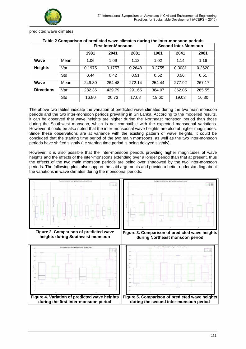
3rd International Symposium on Advances in Civil and Environmental Engineering Practices for Sustainable Development (ACEPS – 2015)
predicted wave climates.
Table 2 Comparison of predicted wave climates during the inter-monsoon periods First Inter-Monsoon Second Inter-Monsoon
1981 2041 2081 1981 2041 2081
Wave
Heights
Mean 1.06 1.09 1.13 1.02 1.14 1.16
Var 0.1975 0.1757 0.2648 0.2755 0.3081 0.2620
Std 0.44 0.42 0.51 0.52 0.56 0.51
Wave
Directions
Mean 249.30 264.48 272.14 254.44 277.92 267.17
Var 282.35 429.79 291.65 384.07 362.05 265.55
Std 16.80 20.73 17.08 19.60 19.03 16.30
The above two tables indicate the variation of predicted wave climates during the two main monsoon periods and the two inter-monsoon periods prevailing in Sri Lanka. According to the modelled results, it can be observed that wave heights are higher during the Northeast monsoon period than those during the Southwest monsoon, which is not compatible with the expected monsoonal variations. However, it could be also noted that the inter-monsoonal wave heights are also at higher magnitudes. Since these observations are at variance with the existing pattern of wave heights, it could be concluded that the starting time period of the two main monsoons, as well as the two inter-monsoon periods have shifted slightly (i.e starting time period is being delayed slightly). However, it is also possible that the inter-monsoon periods providing higher magnitudes of wave heights and the effects of the inter-monsoons extending over a longer period than that at present, thus the effects of the two main monsoon periods are being over shadowed by the two inter-monsoon periods. The following plots also support the said arguments and provide a better understanding about the variations in wave climates during the monsoonal periods.
Figure 2. Comparison of predicted wave
heights during Southwest monsoon
Figure 3. Comparison of predicted wave heights
during Northeast monsoon period
Figure 4. Variation of predicted wave heights
during the first inter-monsoon period
Figure 5. Comparison of predicted wave heights
during the second inter-monsoon period
131
3rd International Symposium on Advances in Civil and Environmental Engineering Practices for Sustainable Development (ACEPS – 2015)
be shared with SWAN. Similarly, SWAN could be readily nested in WAVEWATCH III for collaborative modelling of wave climates from Deep Ocean to shoreline. In this research study, the said similarities have been extensively exploited, in order to couple the WW3 and SWAN together to model the necessary outputs. (Cavaleri et al., 2007), (Chawla & Tolman, 2007), (The SWAN Team, 2010), (The SWAN Team, 2011 (c)), and (The Wave Model Development and Implementation Group, 1988).
5. MODELLED WAVE OUTPUTS
The outputs obtained via wave modelling are for three different time spans, could be identified as the following.
(i) Past wave climate - year 1981 to 2000 (ii) First future wave climate – year 2041 to 2060 (iii) Second future wave climate - year 2081 to 2100)
In order to match with the overall project requirements, outputs were obtained for a point near Colombo. This was also governed by the fact of available wave measurements. Most of the available wave measurements are for Colombo, thus it is convenient to compare the modelled wave output against the available wave measurement. The comparison of the variation in wave climates were carried out with respect to the modelled past wave climate and the comparisons made reviled the fact that there might be a considerable differences in future wave climates along the western coast of Sri Lanka. Comparison of mean wave climates indicates an increment of about 6.5% for projected mean wave height during year 2041 – 2060 and 8.5% increment for the same during year 2081 – 2100. The mean wave direction of the first future wave climate shows an increment of about 8% and that is slightly reduced during the second projected wave climate. Although these are not very alarming in magnitudes, it indicates a significant variation, when considered with respect to the usual seasonal wave climates prevailing in Sri Lanka. The predicted wave climate changes could be considered in correspond to main rainy seasons prevailing in Sri Lanka. Sri Lanka has two major monsoon periods and two inter-monsoon periods, where the time periods are to be considered as the following. • Southwest monsoon – May to September • Northeast monsoon – December to February • First inter-monsoon – October to November • Second inter-monsoon – March to April
Investigating the predicted changes during these major seasons is particularly important, due to the fact that the wave condition along the western coast of Sri Lanka is expected to exhibits major seasonal variations, especially during the southwest monsoon period. Table 1 indicates the predicted wave climates during the two major monsoon periods.
Table 1 Comparison of predicted wave climates during the monsoon periods Southwest Monsoon Northeast Monsoon
1981 2041 2081 1981 2041 2081
Wave
Heights
Mean 1.06 1.12 1.11 1.06 1.14 1.18
Var 0.2047 0.2558 0.2808 0.2401 0.2317 0.2372
Std 0.45 0.51 0.53 0.49 0.48 0.49
Wave
Directions
Mean 249.88 269.84 267.32 247.47 270.12 272.27
Var 279.51 294.81 371.58 291.79 335.40 383.66
Std 16.72 17.17 19.28 17.08 19.31 19.59
Similarly, it is necessary to have a comparison of the predicted wave climates for the two inter-monsoon periods as well. Table 2 consists of the necessary information for the said comparison of
130
3rd International Symposium on Advances in Civil and Environmental Engineering Practices for Sustainable Development (ACEPS – 2015)
Although the work done relating to wave climate with future climate changes are rare to find for the Sri Lankan context, there are number of successful benchmark attempts that have been made in various parts of the world to address the said issue. Almost in all such research work carried out, the outcomes claim a significant relationship between the future wave climate and its forcing conditions that are to be caused by future climate change scenarios. The work done by Hamer et al., 2010a emphasize the fact that insufficient projections of wave climate were available to assess the effects of probable climate change impacts on erosion of the world’s coasts. According to the said work, at present, a considerable research effort is placed into regional ocean wave projections, with forcing conditions derived from a few selected emission scenarios from a few selected GCMs. It has identified several shortcomings of such an approach, as the following.
(i) Limitations of statistical confidence in the projections. (ii) Additional effort requirements in modelling due to repeated model runs. (iii) Laps in the global coverage, including the crucial areas that are most likely to be at risk due to
changing wave conditions. The propose solution given in the said study for this problematic scenario was to shift to global projections. The aim should be to use different wave models and statistical downscaling approaches to produce ensembles of wave projections that correspond to climate projections from different climate models for different emission scenarios. When combined, a distribution of projections will be available that will allow an assessment of all three levels of uncertainty (associated with forcing, climate models, and downscaling methods, respectively), presenting projections within statistical confidence intervals. The proposed design will provide suitable data on a global scale for carrying out surface ocean wave projections, focusing on mid- and late-twenty-first-century time slices, to service the increasing demands of the coastal impacts community. Future studies could include dynamic coupling of wave processes into coupled ocean–atmosphere global climate models (Hamer et al., 2010a). According to work done by Swail & Wang, 2005, results of ocean wave climate change scenarios for the northern hemisphere oceans for the twenty-first century show that significant changes can be anticipated in both the North Atlantic and the North Pacific under all the three forcing-scenarios. The rate and sign of the projected future wave height changes are not constant throughout the 21st century and in some regions, these appear to be very much dependent on the forcing conditions as well. The rate of change appears to have a positive relationship with the rate of increase in the greenhouse-gases forcing.
4. USE OF WAVEWATCH III AND SWAN MODELS TO MODEL FUTURE WAVE CLIMATES
The basic scientific philosophy of SWAN is identical to that of WAM (Cycle 3 and 4) and it uses the same formulations for the source terms. On the other hand, SWAN contains some additional formulations, primarily for shallow water. Moreover, the numerical techniques are very different. WAVEWATCH III not only uses different numerical techniques but also different formulations for the wind input and white capping (The Wave Model Development and Implementation Group, 1988). When SWAN is nested with WAVEWATCH III, it was noted that the boundary conditions for SWAN provided by WAVEWATCH III are not consistent, even the same physics are being used. The potential reasons are manifold such as the differences in numerical techniques employed and implementation for geographic area (spatial and spectral resolutions, coefficients, etc.) (Chawla & Tolman, 2007), (Tolman, 2010), and (Cavaleri et al., 2007). To overcome this issue, the deep-water boundary of SWAN nest was located in WAVEWATCH III, where shallow water effects do not dominate. This is primarily important to avoid the existence of large discontinuities between the two models. At the same time, the spatial and spectral resolutions were adjusted so that it will not differ largely from one another, in order to avoid additional modifications of the model layout (Cavaleri et al., 2007), and (Chawla & Tolman, 2007). Since SWAN in coded in such a manner, so that the scientific findings with another wave model could
129
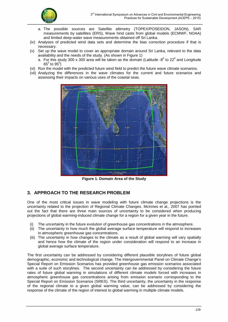
3rd International Symposium on Advances in Civil and Environmental Engineering Practices for Sustainable Development (ACEPS – 2015)
a. The possible sources are Satellite altimetry (TOPEX/POSEIDON, JASON), SAR measurements by satellites (ERS), Wave hind casts from global models (ECMWF, NOAA) and limited deep-water wave measurements obtained off Sri Lanka.
(iv) Analyses of predicted wind data sets and determine the bias correction procedure if that is necessary.
(v) Set up the wave model to cover an appropriate domain around Sri Lanka, relevant to the data availability and the needs of the study. (As shown in Figure 1) a. For this study 300 x 300 area will be taken as the domain (Latitude -80 to 220 and Longitude
650 to 950) (vi) Run the model with the predicted future wind field to predict the future wave climate scenarios. (vii) Analyzing the differences in the wave climates for the current and future scenarios and
assessing their impacts on various uses of the coastal seas.
Figure 1. Domain Area of the Study
3. APPROACH TO THE RESEARCH PROBLEM
One of the most critical issues in wave modeling with future climate change projections is the uncertainty related to the projection of Regional Climate Changes. McInnes et al., 2007 has pointed out the fact that there are three main sources of uncertainty to be considered when producing projections of global warming-induced climate change for a region for a given year in the future.
(i) The uncertainty in the future evolution of greenhouse gas concentrations in the atmosphere. (ii) The uncertainty in how much the global average surface temperature will respond to increases
in atmospheric greenhouse gas concentrations. (iii) The uncertainty in how changes to the climate as a result of global warming will vary spatially
and hence how the climate of the region under consideration will respond to an increase in global average surface temperature.
The first uncertainty can be addressed by considering different plausible storylines of future global demographic, economic and technological change. The Intergovernmental Panel on Climate Change’s Special Report on Emission Scenarios has provided greenhouse gas emission scenarios associated with a suite of such storylines. The second uncertainty can be addressed by considering the future rates of future global warming in simulations of different climate models forced with increases in atmospheric greenhouse gas concentrations arising from emission scenario corresponding to the Special Report on Emission Scenarios (SRES). The third uncertainty, the uncertainty in the response of the regional climate to a given global warming value, can be addressed by considering the response of the climate of the region of interest to global warming in multiple climate models.
128
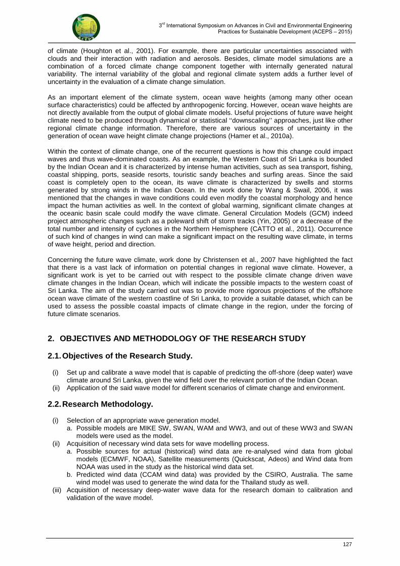
3rd International Symposium on Advances in Civil and Environmental Engineering Practices for Sustainable Development (ACEPS – 2015)
of climate (Houghton et al., 2001). For example, there are particular uncertainties associated with clouds and their interaction with radiation and aerosols. Besides, climate model simulations are a combination of a forced climate change component together with internally generated natural variability. The internal variability of the global and regional climate system adds a further level of uncertainty in the evaluation of a climate change simulation. As an important element of the climate system, ocean wave heights (among many other ocean surface characteristics) could be affected by anthropogenic forcing. However, ocean wave heights are not directly available from the output of global climate models. Useful projections of future wave height climate need to be produced through dynamical or statistical ‘‘downscaling’’ approaches, just like other regional climate change information. Therefore, there are various sources of uncertainty in the generation of ocean wave height climate change projections (Hamer et al., 2010a). Within the context of climate change, one of the recurrent questions is how this change could impact waves and thus wave-dominated coasts. As an example, the Western Coast of Sri Lanka is bounded by the Indian Ocean and it is characterized by intense human activities, such as sea transport, fishing, coastal shipping, ports, seaside resorts, touristic sandy beaches and surfing areas. Since the said coast is completely open to the ocean, its wave climate is characterized by swells and storms generated by strong winds in the Indian Ocean. In the work done by Wang & Swail, 2006, it was mentioned that the changes in wave conditions could even modify the coastal morphology and hence impact the human activities as well. In the context of global warming, significant climate changes at the oceanic basin scale could modify the wave climate. General Circulation Models (GCM) indeed project atmospheric changes such as a poleward shift of storm tracks (Yin, 2005) or a decrease of the total number and intensity of cyclones in the Northern Hemisphere (CATTO et al., 2011). Occurrence of such kind of changes in wind can make a significant impact on the resulting wave climate, in terms of wave height, period and direction. Concerning the future wave climate, work done by Christensen et al., 2007 have highlighted the fact that there is a vast lack of information on potential changes in regional wave climate. However, a significant work is yet to be carried out with respect to the possible climate change driven wave climate changes in the Indian Ocean, which will indicate the possible impacts to the western coast of Sri Lanka. The aim of the study carried out was to provide more rigorous projections of the offshore ocean wave climate of the western coastline of Sri Lanka, to provide a suitable dataset, which can be used to assess the possible coastal impacts of climate change in the region, under the forcing of future climate scenarios.
2. OBJECTIVES AND METHODOLOGY OF THE RESEARCH STUDY
2.1. Objectives of the Research Study.
(i) Set up and calibrate a wave model that is capable of predicting the off-shore (deep water) wave climate around Sri Lanka, given the wind field over the relevant portion of the Indian Ocean.
(ii) Application of the said wave model for different scenarios of climate change and environment. 2.2. Research Methodology.
(i) Selection of an appropriate wave generation model. a. Possible models are MIKE SW, SWAN, WAM and WW3, and out of these WW3 and SWAN
models were used as the model. (ii) Acquisition of necessary wind data sets for wave modelling process.
a. Possible sources for actual (historical) wind data are re-analysed wind data from global models (ECMWF, NOAA), Satellite measurements (Quickscat, Adeos) and Wind data from NOAA was used in the study as the historical wind data set.
b. Predicted wind data (CCAM wind data) was provided by the CSIRO, Australia. The same wind model was used to generate the wind data for the Thailand study as well.
(iii) Acquisition of necessary deep-water wave data for the research domain to calibration and validation of the wave model.
127
3rd International Symposium on Advances in Civil and Environmental Engineering Practices for Sustainable Development (ACEPS – 2015)
Climate Change Impacts on Seasonal Wave Climate of the Western Coast of Sri Lanka
R. M. J. Bamunawala1, S. S. L. Hettiarachchi2, S. P. Samarawickrama2,
P. N. Wickramanayakkara3, Roshanka Ranasinghe4
1Department of Civil Engineering, University of Moratuwa, Sri Lanka
2Department of Civil Engineering, University of Moratuwa, Sri Lanka
3Department of Civil Engineering, Open University Sri Lanka, Sri Lanka.
4Department of Water Engineering, UNESCO–IHE, Delft, The Netherlands
E-mail: [email protected] Abstract: Climate change and climate change driven impacts are most widely argued topics among contemporary researchers and scientists. Broadly there are two schools of philosophies that process entirely contrasting concepts about this whole concept of climate change and its impacts. While one of the concepts state about frequently varied climate change and occurrence of extreme weather events the others are banking upon the concept that there is no climate change and it is only the indifferences in occurrence of weather and climate events. The title of this study itself implies the fact that this research study supports the concept of climate change and its probable impacts, thus leaving out the other approach on climate change. Extensive concentrations of green house gasses emitted to the earth’s atmosphere and vast amounts of aerosols govern the majority of anthropogenic causes for climate change, while many of the natural causes such as changes in solar radiation also contribute immensely to earth’s climate change. Absence of detailed studies carried out on investigating probable impacts on wave climates due to projected climate changes is one of the major drawbacks in handling the unique coastal eco systems in Sri Lanka. As a country where coastal resources play a major role in its development, it is absolutely necessary to have a clear idea about the probable impacts that could arise on its coastal areas. This detailed investigation provides vital information on probable impacts that might cause on the western coast of Sri Lanka under the influence of global climate change.The outcomes of this study indicate that there is certain threat to the coasts in Sri Lanka due to a considerable increment in mean wave height and shifted wave directions. It also indicates that not only the number of extreme wave events increase very significantly but also its intensity upsurges in a considerable amount as well, while indicating a major shift in seasonal wave climate that prevails along the western coast of Sri Lanka. This probable shift of seasonal wave climate of the western coast should be considered seriously, since many of its socio-economic activities are directly related to this seasonal wave climate variation. Keywords: Climate Change impacts, seasonal wave climate shift, mean wave height and direction
1. INTRODUCTION
Changes in the Earth’s climate and its possible impacts belong to most widely discussed scientific problems in the present era. These climate changes occur due to both internal variability within the climate system and external factors, which can be either anthropogenic or natural. Increasing concentration of atmospheric greenhouse-gases tends to warm the Earth’s surface and its lower atmosphere, while an increase in some types of aerosols tends to cool it (Houghton et al., 2001). Natural factors, such as changes in solar output or explosive volcanic activity, can also cause radioactive forcing and hence influence the Earth’s climate. Complex climate models are required to provide detailed estimates of feedbacks and regional features in the climate system. Although confidence in the ability of these models to provide useful projections of future climate has improved on a range of space and time-scales, the present-day climate models cannot yet simulate all aspects
126
3rd International Symposium on Advances in Civil and Environmental Engineering Practices for Sustainable Development (ACEPS – 2015)
5. CONCLUSION
The present formula derived for the recession seems to be superior to the existing formulae considered in this study based on the following reasons.
• The threshold condition where zero recession occurs in actual cases is addressed and solved to a certain degree in the present formula.
• Gives more accurate results for the model test data sets considered. However, the present formula could be further improved using more test results. Following improvements are recommended.
• The proposed formula should be validated using independent test results. • The effect of the parameter such as N, h, hberm, etc. needs to be incorporated. • Actual test conditions used to derive different formulae considered in this study should be
taken into consideration in the comparison of results. 6. ACKNOWLEDGEMENT Sincere gratitude goes to Mr. N.M.T.K Revel for his contribution through advising on the concept of the research and helping with wave data extraction and data analysis. 7. REFERENCES Andersen T.L. (2006). Hydraulic Response of Rubble Mound Breakwaters. PhD. Thesis. Aalborg University.
Andersen T.L. and Burcharth H.F. (2009). A New Formula for Front Slope Recession of Berm Breakwaters. Coast. Eng. Journal. Elsevier. 57 (4). 359–374.
Goda Y. and Suzuki Y. (1976). Estimation of incident and reflected wave in random wave experiments. Proc.15th International Conf., Hawai. 828–844.
Hall K. and Kao S. (1991). A Study of the Stability of Dynamically Stable Breakwaters. Canadian Journal of Civil Engineering. 18.916 – 925.
Moghim M.N., Shafiefar M., Chegini V. and Aghtouman P. (2009). Effects of Irregular Wave Parameters on Berm Recession of Reshaping Berm Breakwaters. International Journal of Maritime Technology. 5 (9). 35-51.
PIANC (2003), State of the Art of Designing and Constructing Berm Breakwaters, International Navigation Association, PIANC, Brussels.
Sigurdarson S. (2013). Design of Berm Breakwaters: Recession, Overtopping and Reflection, Icebreak Consulting Engineers ehf, Reykjavik, Iceland Jentsje van der Meer, Van der Meer Consulting BV, Akkrum, The Netherlands.
Sigurdarson S., van der Meer J.W., Burcharth H.F. and Sørensen J.D. (2007). Optimum safety levels and design rules for the Icelandic type berm breakwater. Proc. Coastal Structures, Venice, Italy.
Tørum A. and Krogh S.R. (2000). Berm breakwaters. Stone quality. SINTEF Report No. STF22 A00207, to the Norwegian Coast Directorate.
125
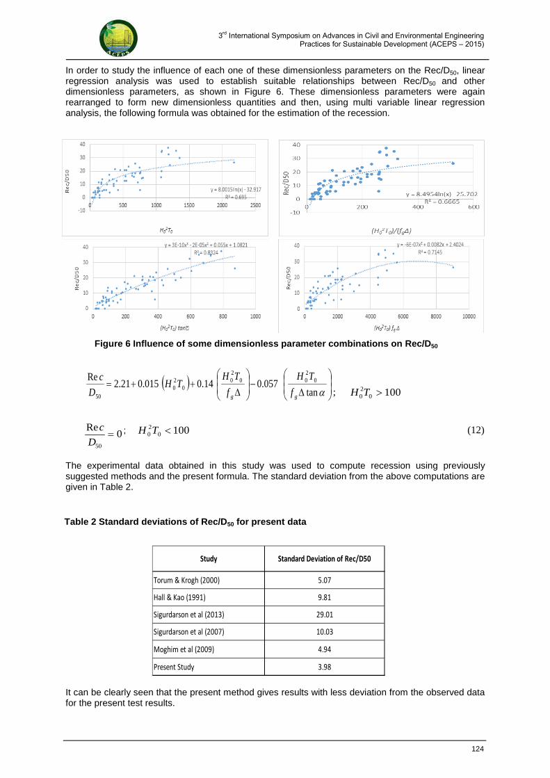
3rd International Symposium on Advances in Civil and Environmental Engineering Practices for Sustainable Development (ACEPS – 2015)
In order to study the influence of each one of these dimensionless parameters on the Rec/D50, linear regression analysis was used to establish suitable relationships between Rec/D50 and other dimensionless parameters, as shown in Figure 6. These dimensionless parameters were again rearranged to form new dimensionless quantities and then, using multi variable linear regression analysis, the following formula was obtained for the estimation of the recession.
For 1000
20 >TH ; For ; 1000
20 >TH
For ; 1000
20 <TH (12)
The experimental data obtained in this study was used to compute recession using previously suggested methods and the present formula. The standard deviation from the above computations are given in Table 2.
It can be clearly seen that the present method gives results with less deviation from the observed data for the present test results.
Figure 6 Influence of some dimensionless parameter combinations on Rec/D50
( )
∆−
∆++=
αtan057.014.0015.021.2
Re 0200
20
020
50 gg f
TH
f
THTH
D
c
0Re
50
=D
c
Table 2 Standard deviations of Rec/D50 for present data
Study Standard Deviation of Rec/D50
Torum & Krogh (2000) 5.07
Moghim et al (2009) 4.94
Present Study 3.98
Hall & Kao (1991) 9.81
Sigurdarson et al (2013) 29.01
Sigurdarson et al (2007) 10.03
124
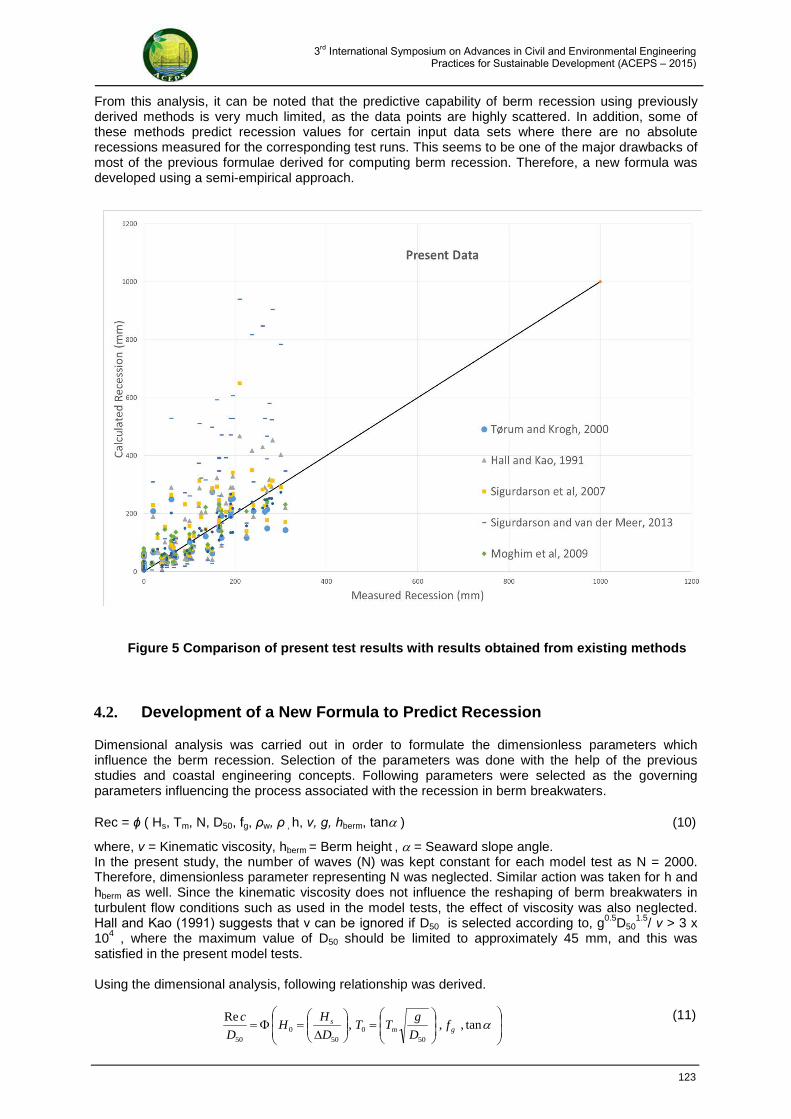
3rd International Symposium on Advances in Civil and Environmental Engineering Practices for Sustainable Development (ACEPS – 2015)
From this analysis, it can be noted that the predictive capability of berm recession using previously derived methods is very much limited, as the data points are highly scattered. In addition, some of these methods predict recession values for certain input data sets where there are no absolute recessions measured for the corresponding test runs. This seems to be one of the major drawbacks of most of the previous formulae derived for computing berm recession. Therefore, a new formula was developed using a semi-empirical approach.
4.2. Development of a New Formula to Predict Recession
Dimensional analysis was carried out in order to formulate the dimensionless parameters which influence the berm recession. Selection of the parameters was done with the help of the previous studies and coastal engineering concepts. Following parameters were selected as the governing parameters influencing the process associated with the recession in berm breakwaters. Rec = ϕ ( Hs, Tm, N, D50, fg, ρw, ρ , h, ν, g, hberm, tanα ) (10)
where, ν = Kinematic viscosity, hberm = Berm height , α = Seaward slope angle. In the present study, the number of waves (N) was kept constant for each model test as N = 2000. Therefore, dimensionless parameter representing N was neglected. Similar action was taken for h and hberm as well. Since the kinematic viscosity does not influence the reshaping of berm breakwaters in turbulent flow conditions such as used in the model tests, the effect of viscosity was also neglected. Hall and Kao (1991) suggests that ν can be ignored if D50 is selected according to, g0.5D50
1.5/ ν > 3 x 10⁴ , where the maximum value of D50 should be limited to approximately 45 mm, and this was satisfied in the present model tests. Using the dimensional analysis, following relationship was derived.
(11)
Figure 5 Comparison of present test results with results obtained from existing methods
=
∆
=Φ= αtan,,,Re
500
500
50gm
s fD
gTT
D
HH
D
c
123
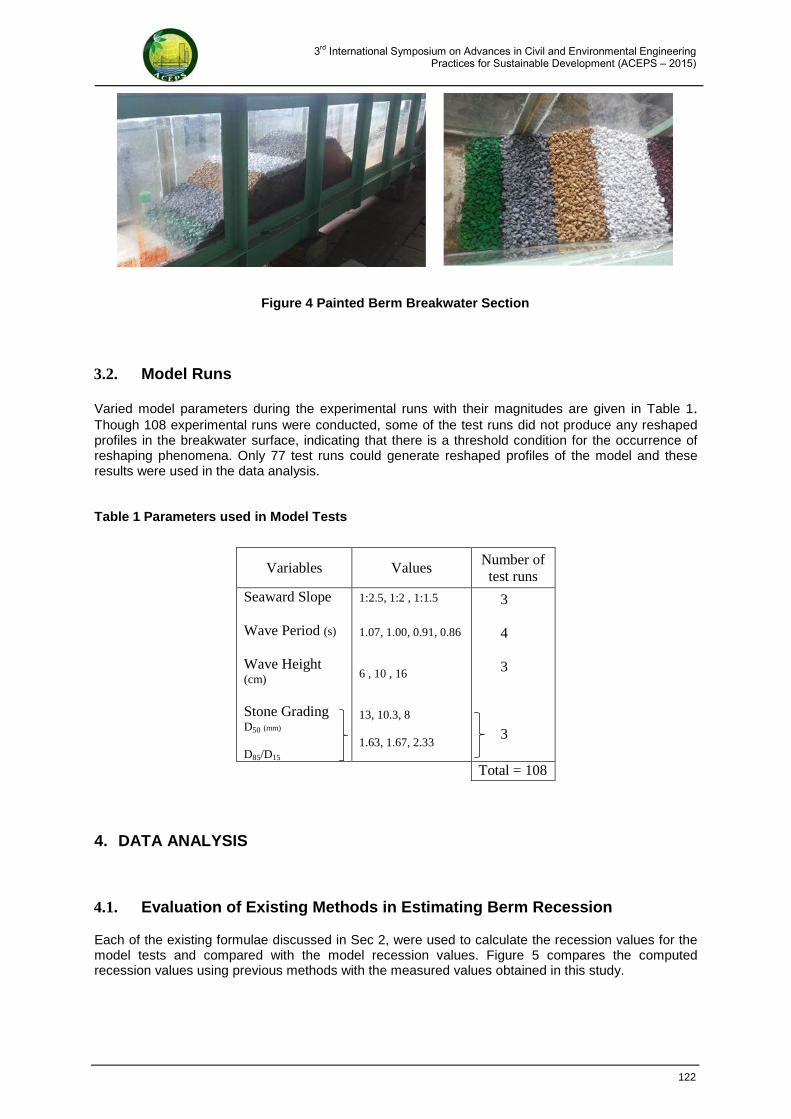
3rd International Symposium on Advances in Civil and Environmental Engineering Practices for Sustainable Development (ACEPS – 2015)
3.2. Model Runs
Varied model parameters during the experimental runs with their magnitudes are given in Table 1. Though 108 experimental runs were conducted, some of the test runs did not produce any reshaped profiles in the breakwater surface, indicating that there is a threshold condition for the occurrence of reshaping phenomena. Only 77 test runs could generate reshaped profiles of the model and these results were used in the data analysis. Table 1 Parameters used in Model Tests
4. DATA ANALYSIS
4.1. Evaluation of Existing Methods in Estimating Berm Recession
Each of the existing formulae discussed in Sec 2, were used to calculate the recession values for the model tests and compared with the model recession values. Figure 5 compares the computed recession values using previous methods with the measured values obtained in this study.
Variables Values Number of test runs
Seaward Slope Wave Period (s)
Wave Height (cm) Stone Grading D50 (mm) D85/D15
1:2.5, 1:2 , 1:1.5
1.07, 1.00, 0.91, 0.86
6 , 10 , 16 13, 10.3, 8 1.63, 1.67, 2.33
3 4 3 3
Total = 108
Figure 4 Painted Berm Breakwater Section
122
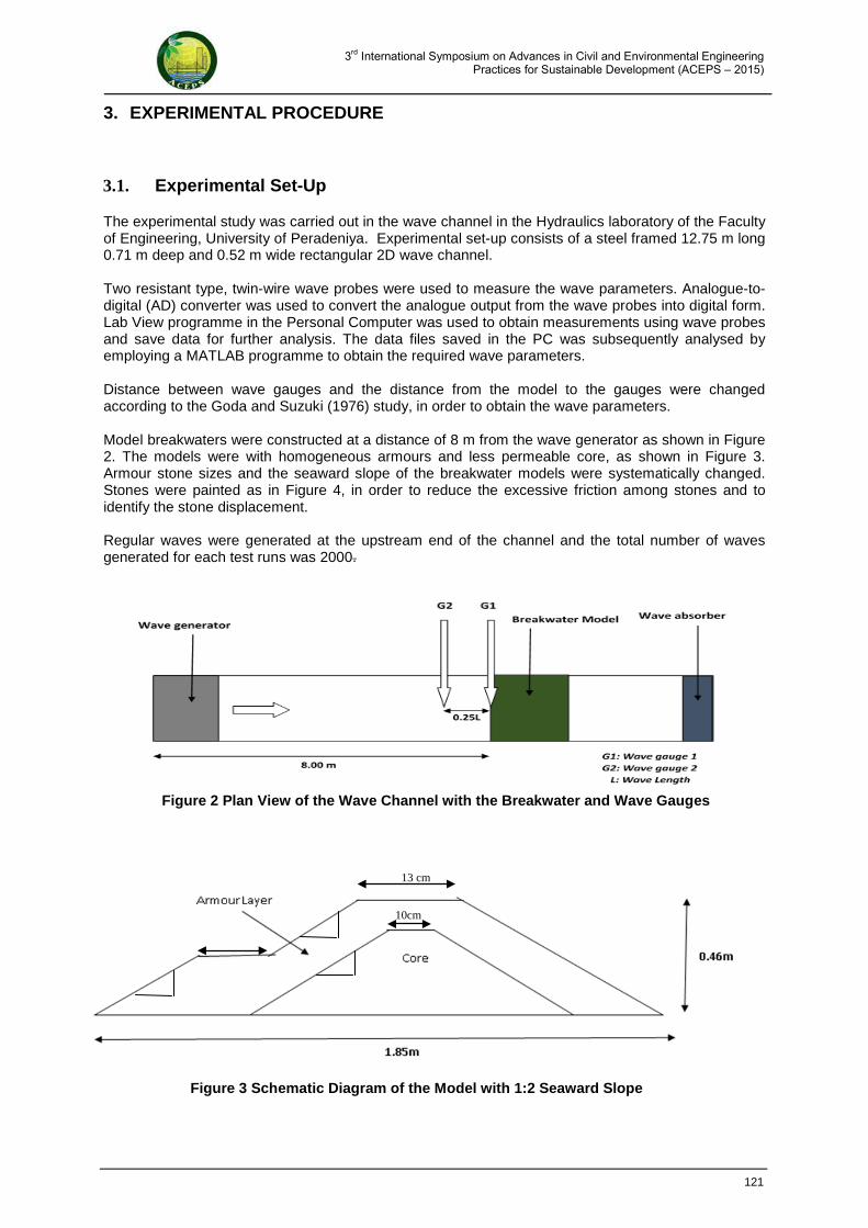
3rd International Symposium on Advances in Civil and Environmental Engineering Practices for Sustainable Development (ACEPS – 2015)
Figure 3 Schematic Diagram of the Model with 1:2 Seaward Slope
13 cm
10cm
3. EXPERIMENTAL PROCEDURE
3.1. Experimental Set-Up
The experimental study was carried out in the wave channel in the Hydraulics laboratory of the Faculty of Engineering, University of Peradeniya. Experimental set-up consists of a steel framed 12.75 m long 0.71 m deep and 0.52 m wide rectangular 2D wave channel. Two resistant type, twin-wire wave probes were used to measure the wave parameters. Analogue-to-digital (AD) converter was used to convert the analogue output from the wave probes into digital form. Lab View programme in the Personal Computer was used to obtain measurements using wave probes and save data for further analysis. The data files saved in the PC was subsequently analysed by employing a MATLAB programme to obtain the required wave parameters. Distance between wave gauges and the distance from the model to the gauges were changed according to the Goda and Suzuki (1976) study, in order to obtain the wave parameters. Model breakwaters were constructed at a distance of 8 m from the wave generator as shown in Figure 2. The models were with homogeneous armours and less permeable core, as shown in Figure 3. Armour stone sizes and the seaward slope of the breakwater models were systematically changed. Stones were painted as in Figure 4, in order to reduce the excessive friction among stones and to identify the stone displacement. Regular waves were generated at the upstream end of the channel and the total number of waves generated for each test runs was 2000.
Figure 2 Plan View of the Wave Channel with the Breakwater and Wave Gauges
121
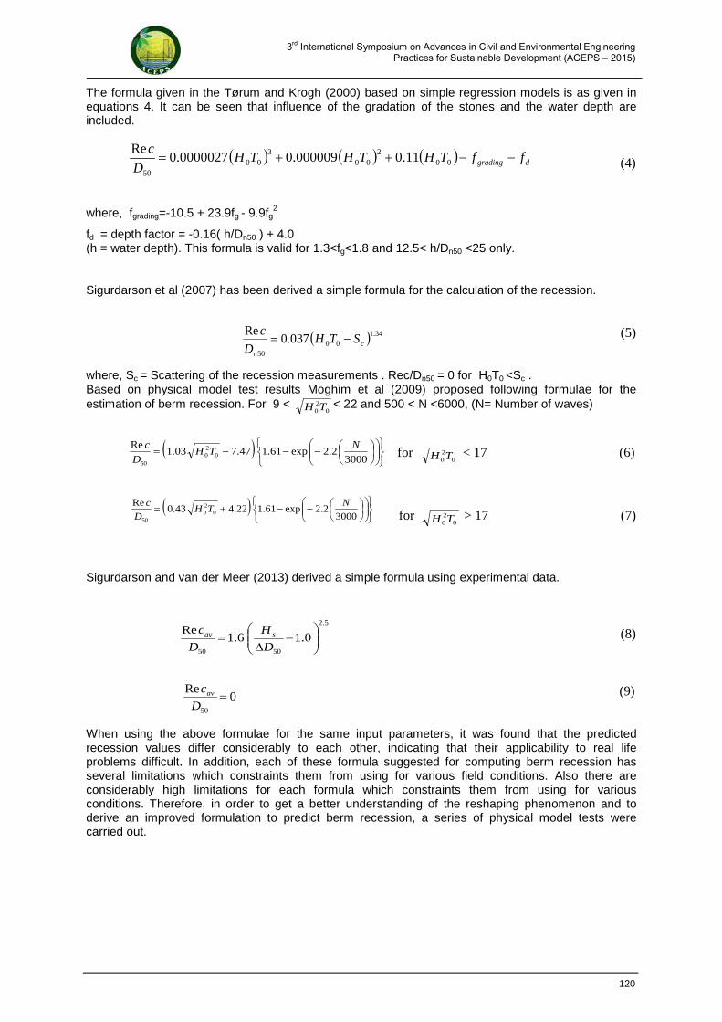
3rd International Symposium on Advances in Civil and Environmental Engineering Practices for Sustainable Development (ACEPS – 2015)
The formula given in the Tørum and Krogh (2000) based on simple regression models is as given in equations 4. It can be seen that influence of the gradation of the stones and the water depth are included.
(4)
where, fgrading=-10.5 + 23.9fg - 9.9fg2
fd = depth factor = -0.16( h/Dn50 ) + 4.0 (h = water depth). This formula is valid for 1.3<fg<1.8 and 12.5< h/Dn50 <25 only. Sigurdarson et al (2007) has been derived a simple formula for the calculation of the recession.
(5)
where, Sc = Scattering of the recession measurements . Rec/Dn50 = 0 for H0T0 <Sc . Based on physical model test results Moghim et al (2009) proposed following formulae for the estimation of berm recession. For 9 <
020TH < 22 and 500 < N <6000, (N= Number of waves)
for
020TH < 17 (6)
for
020TH > 17 (7)
Sigurdarson and van der Meer (2013) derived a simple formula using experimental data.
(8)
(9)
When using the above formulae for the same input parameters, it was found that the predicted recession values differ considerably to each other, indicating that their applicability to real life problems difficult. In addition, each of these formula suggested for computing berm recession has several limitations which constraints them from using for various field conditions. Also there are considerably high limitations for each formula which constraints them from using for various conditions. Therefore, in order to get a better understanding of the reshaping phenomenon and to derive an improved formulation to predict berm recession, a series of physical model tests were carried out.
( ) ( ) ( ) dgrading ffTHTHTHD
c−−++= 00
200
300
50
11.0000009.00000027.0Re
( ) 34.100
50
037.0Re
cn
STHD
c−=
( )
−−−=
30002.2exp61.147.703.1
Re0
20
50
NTH
D
c
( )
−−+=
30002.2exp61.122.443.0
Re0
20
50
NTH
D
c
5.2
5050
0.16.1Re
−
∆=
D
H
D
c sav
0Re
50
=D
cav
120
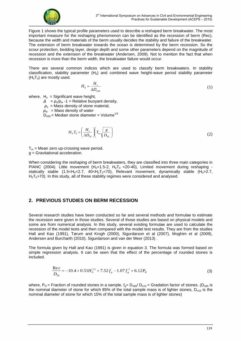
3rd International Symposium on Advances in Civil and Environmental Engineering Practices for Sustainable Development (ACEPS – 2015)
Figure 1 shows the typical profile parameters used to describe a reshaped berm breakwater. The most important measure for the reshaping phenomenon can be identified as the recession of berm (Rec), because the width and materials of the berm usually decides the stability and failure of the breakwater. The extension of berm breakwater towards the ocean is determined by the berm recession. So the scour protection, bedding layer, design depth and some other parameters depend on the magnitude of recession and the extension of the breakwater (Andersen, 2009). Not to mention the fact that when recession is more than the berm width, the breakwater failure would occur. There are several common indices which are used to classify berm breakwaters. In stability classification, stability parameter (H0) and combined wave height-wave period stability parameter (H0T0) are mostly used.
(1)
where, Hs = Significant wave height, Δ = ρs/ρw -1 = Relative buoyant density, ρs = Mass density of stone material, ρw = Mass density of water Dn50 = Median stone diameter = Volume1/3
(2)
Tm = Mean zero up-crossing wave period. g = Gravitational acceleration. When considering the reshaping of berm breakwaters, they are classified into three main categories in PIANC (2004). Little movement (H0<1.5-2, H0T0 <20-40), Limited movement during reshaping - statically stable (1.5<H0<2.7, 40<H0T0<70), Relevant movement, dynamically stable (H0>2.7, H0T0>70). In this study, all of these stability regimes were considered and analysed.
2. PREVIOUS STUDIES ON BERM RECESSION
Several research studies have been conducted so far and several methods and formulae to estimate the recession were given in those studies. Several of those studies are based on physical models and some are from numerical analysis. In this study, several existing formulae are used to calculate the recession of the model tests and then compared with the model test results. They are from the studies Hall and Kao (1991), Tørum and Krogh (2000), Sigurdarson et al (2007), Moghim et al (2009), Andersen and Burcharth (2010), Sigurdarson and van der Meer (2013) . The formula given by Hall and Kao (1991) is given in equation 3. The formula was formed based on simple regression analysis. It can be seen that the effect of the percentage of rounded stones is included.
(3)
where, PR = Fraction of rounded stones in a sample, fg= Dn85/ Dn15 = Gradation factor of stones. (Dn85 is the nominal diameter of stone for which 85% of the total sample mass is of lighter stones, Dn15 is the nominal diameter of stone for which 15% of the total sample mass is of lighter stones)
Rgg PffHD
c12.607.152.751.04.10
Re 25.20
50
+−++−=
500
n
s
D
HH
∆=
∆
=5050
00 D
gT
D
HTH m
s
119
3rd International Symposium on Advances in Civil and Environmental Engineering Practices for Sustainable Development (ACEPS – 2015)
An Experimental Study on Berm Breakwater Recession
M.M.G.D. Madakumbura1, D.A.A. Niroshan1, P.D.H.S. Pathirage1 and K.P.P. Pathirana1
1Department of Civil Engineering, Faculty of Engineering, University of Peradeniya,
SRI LANKA
E-Mail: [email protected] Abstract: Berm Breakwaters are allowed to reshape its seaward profile of the breakwater to a more stable profile that could effectively withstand the wave action and the reshaped profile parameters are very crucial when designing a berm breakwater. Berm Recession can be identified as one of the most important profile parameters and In this study, influence of various parameters on berm recession was studied based on the two dimensional model tests carried out at the Faculty of Engineering, University of Peradeniya. A new formula for recession was derived using dimensional analysis and it was compared with the existing formulae. Keywords: Berm Breakwaters, Recession, Physical Model Tests, Waves
1. INTRODUCTION
Berm breakwaters are different from other conventional breakwaters because conventional breakwaters are almost statically stable whereas, the seaward slope of berm breakwaters are allowed to reshape to a stable profile. Smaller sizes of stones can be used for berm breakwaters because they are allowed to reshape. Compared to conventional rubble mound breakwaters, 2 to 10 times smaller stones can be used for berm breakwaters. Berm breakwaters can also be constructed by using relatively easy, land based methods and less specialized construction equipment compared to conventional breakwaters, therefore, low cost can be considered as an added advantage. As a berm breakwater dissipates much of the wave energy with minimum reflection, smaller vessels can navigate very close to berm breakwaters.
Though berm breakwaters have many advantages, very few berm breakwaters are reported to be constructed around the world. According to the report of working group 40 of the PIANC (2003), only around 60 berm breakwaters had been constructed before 2004. This type of breakwaters is mainly used in Iceland, Norway and Denmark. Lack of experience in berm breakwaters and the consideration of higher risk of failure compared to conventional breakwaters due to excessive reshaping and changes of sections as a result of not having clear design guidelines, could be some of the reasons for less popularity of berm breakwaters. Only limited numbers of studies have been done so far on the stability and reshaping characteristics of berm breakwaters. Therefore, in order to understand some of these phenomena that could eventually be used for improving the design guidelines of berm breakwaters, further studies related to above phenomenon are necessary.
Figure 1 Reshaped profile parameters (after Andersen, 2006)
118
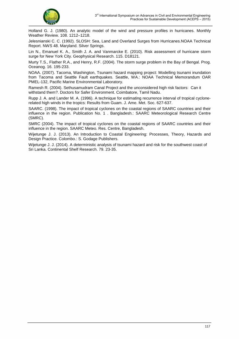
3rd International Symposium on Advances in Civil and Environmental Engineering Practices for Sustainable Development (ACEPS – 2015)
Holland G. J. (1980). An analytic model of the wind and pressure profiles in hurricanes. Monthly Weather Review. 108. 1212–1218.
Jelesnianski C. C. (1992). SLOSH: Sea, Land and Overland Surges from Hurricanes.NOAA Technical Report. NWS 48. Maryland. Silver Springs.
Lin N., Emanuel K. A., Smith J. A. and Vanmarcke E. (2010). Risk assessment of hurricane storm surge for New York City. Geophysical Research. 115. D18121.
Murty T.S., Flather R.A., and Henry, R.F. (2004). The storm surge problem in the Bay of Bengal. Prog. Oceanog. 16. 195-233.
NOAA. (2007). Tacoma, Washington, Tsunami hazard mapping project: Modelling tsunami inundation from Tacoma and Seattle Fault earthquakes. Seattle, WA.: NOAA Technical Memorandum OAR PMEL-132, Pacific Marine Environmental Laboratory.
Ramesh R. (2004). Sethusamudram Canal Project and the unconsidered high risk factors: Can it withstand them?. Doctors for Safer Environment. Coimbatore, Tamil Nadu.
Rupp J. A. and Lander M. A. (1996). A technique for estimating recurrence interval of tropical cyclone-related high winds in the tropics: Results from Guam. J. Ame. Met. Soc. 627-637.
SAARC. (1998). The impact of tropical cyclones on the coastal regions of SAARC countries and their influence in the region. Publication No. 1 . Bangladesh.: SAARC Meteorological Research Centre (SMRC).
SMRC (2004). The impact of tropical cyclones on the coastal regions of SAARC countries and their influence in the region. SAARC Meteo. Res. Centre, Bangladesh.
Wijetunge J. J. (2013). An Introduction to Coastal Engineering: Processes, Theory, Hazards and Design Practice. Colombo.: S. Godage Publishers.
Wijetunge J. J. (2014). A deterministic analysis of tsunami hazard and risk for the southwest coast of Sri Lanka. Continental Shelf Research. 79. 23-35.
117
3rd International Symposium on Advances in Civil and Environmental Engineering Practices for Sustainable Development (ACEPS – 2015)
A field survey of the study area revealed that part of the inundation zone is heavily populated with many residential buildings and commercial establishments; moreover, vital infrastructure such as hospitals, fire stations, electricity sub-stations, schools, etc are also located in the inundation zone. It is proposed that the storm surge risk mitigation strategy for the pilot study area should comprise cyclone and storm surge forecasting, provision of early warning to vulnerable communities to enable their evacuation as well as education and awareness programs at the community level. Finally, there are certain limitations inherent in a study of this nature. One limitation is that the resolution of the modeling is no greater or more accurate than the bathymetric data used. Moreover, the tide has been linearly superimposed on the computed storm surge levels on a conservative basis although the tide-surge interaction is non-linear. It must also be added that the set-up due to wave breaking has not been incorporated in the present model simulations. It must also be added that depth-averaged models assume a uniform velocity profile across the flow depth and neglect vertical accelerations. Moreover, the mathematical formulation employed in the present model does not explicitly account for all means of energy dissipation. For instance, although energy dissipation due to bottom friction is included in the present model, dissipation due to turbulence is not explicitly formulated.
4. CONCLUSIONS
Numerical simulations have been performed to compute the spatial distribution of onshore flooding due to tropical cyclone induced storm surges in Tangalle on the south coast of Sri Lanka, corresponding to a ‘worst-case’ scenario as a pilot study. The effect of the tide has also been incorporated in inundation computations. The simulated flood depths as well as the available vulnerability indicators have been used to delineate the distribution of relative risk to population and dwellings. The effects of the terrain as well as the presence of waterways and water bodies can be seen in the flood distribution in the study area.
5. ACKNOWLEDGEMENT
The authors acknowledge the support received from the National Science Foundation Grant No. RG/2011/ESA/01.
6. REFERENCES
CDM (1964). Ceylon Daily Mirror. Ceylon Daily Mirror Newspaper of 29 December 1964. Times of Ceylon, Colombo.
Chittibabu P. , Dube S. K. , Sinha P. C. , Rao A. D. and Murty T. S. (2002). Numerical Simulation of Extreme Sea Levels for the Tamil Nadu (India) and Sri Lankan Coasts. Marine Geodesy. 25(3).235-244. DMSL (2010). Department of Meteorology, Sri Lanka. Tropical cyclones; Cyclone events 1900-2000. Department of Meteorology, Government of Sri Lanka, http://www.meteo.gov.lk/, accessed on 15-7-2013.
Dube S. K. (2003). Storm surge forecasting in the Bay of Bengal and Arabian Sea. Goa, India.: In Antarctic Geoscience, Ocean-Atmosphere Interaction and Paleoclimatology (Eds. S. Rajan and P.C. Pandey), National Centre for Antarctic & Ocean Research. Gumbel E.J. (1958). Statistics of Extremes. Columbia University Press. New York.
Henry R.F. and T.S. Murty (1992). Storm surges and tides around Sri Lanka. Recent advance in Marine science and technology. 92. 205-218.
116
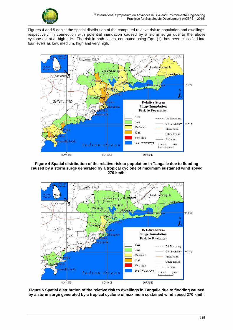
3rd International Symposium on Advances in Civil and Environmental Engineering Practices for Sustainable Development (ACEPS – 2015)
Figures 4 and 5 depict the spatial distribution of the computed relative risk to population and dwellings, respectively, in connection with potential inundation caused by a storm surge due to the above cyclone event at high tide. The risk in both cases, computed using Eqn. (1), has been classified into four levels as low, medium, high and very high.
Figure 4 Spatial distribution of the relative risk to population in Tangalle due to flooding
caused by a storm surge generated by a tropical cyclone of maximum sustained wind speed 270 km/h.
Figure 5 Spatial distribution of the relative risk to dwellings in Tangalle due to flooding caused by a storm surge generated by a tropical cyclone of maximum sustained wind speed 270 km/h.
115
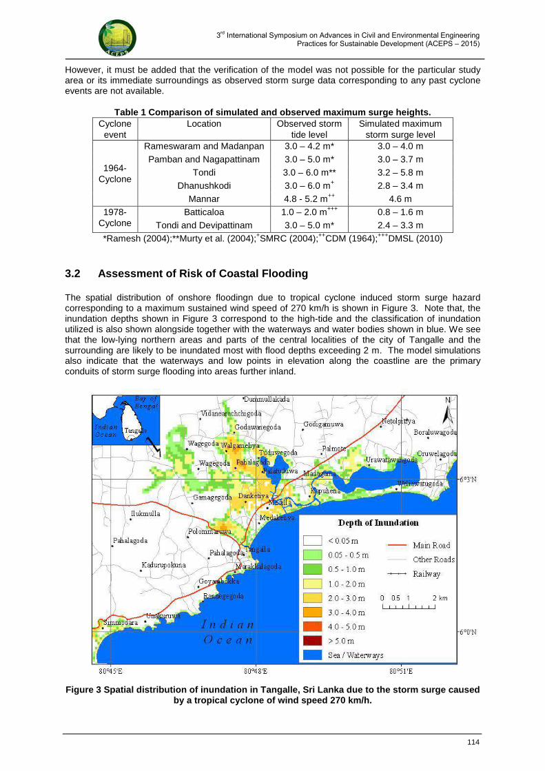
3rd International Symposium on Advances in Civil and Environmental Engineering Practices for Sustainable Development (ACEPS – 2015)
However, it must be added that the verification of the model was not possible for the particular study area or its immediate surroundings as observed storm surge data corresponding to any past cyclone events are not available.
Table 1 Comparison of simulated and observed maximum surge heights. Cyclone
event Location Observed storm
tide level Simulated maximum
storm surge level
1964-Cyclone
Rameswaram and Madanpan 3.0 – 4.2 m*
3.0 – 4.0 m
Pamban and Nagapattinam 3.0 – 5.0 m*
3.0 – 3.7 m
Tondi 3.0 – 6.0 m**
3.2 – 5.8 m
Dhanushkodi 3.0 – 6.0 m+
2.8 – 3.4 m
Mannar 4.8 - 5.2 m++
4.6 m
1978-Cyclone
Batticaloa 1.0 – 2.0 m+++
0.8 – 1.6 m
Tondi and Devipattinam 3.0 – 5.0 m*
2.4 – 3.3 m
*Ramesh (2004);**Murty et al. (2004);+SMRC (2004);++CDM (1964);+++DMSL (2010) 3.2 Assessment of Risk of Coastal Flooding
The spatial distribution of onshore floodingn due to tropical cyclone induced storm surge hazard corresponding to a maximum sustained wind speed of 270 km/h is shown in Figure 3. Note that, the inundation depths shown in Figure 3 correspond to the high-tide and the classification of inundation utilized is also shown alongside together with the waterways and water bodies shown in blue. We see that the low-lying northern areas and parts of the central localities of the city of Tangalle and the surrounding are likely to be inundated most with flood depths exceeding 2 m. The model simulations also indicate that the waterways and low points in elevation along the coastline are the primary conduits of storm surge flooding into areas further inland.
Figure 3 Spatial distribution of inundation in Tangalle, Sri Lanka due to the storm surge caused by a tropical cyclone of wind speed 270 km/h.
114
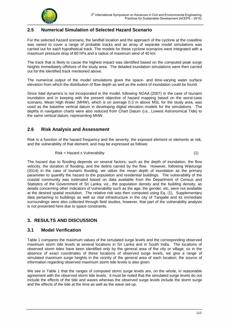
3rd International Symposium on Advances in Civil and Environmental Engineering Practices for Sustainable Development (ACEPS – 2015)
2.5 Numerical Simulation of Selected Hazard Scenario
For the selected hazard scenario, the landfall location and the approach of the cyclone at the coastline was varied to cover a range of probable tracks and an array of separate model simulations was carried out for each hypothetical track. The models for these cyclone scenarios were integrated with a maximum pressure drop of 80 hPa and a radius of maximum wind of 40 km. The track that is likely to cause the highest impact was identified based on the computed peak surge heights immediately offshore of the study area. The detailed inundation simulations were then carried out for the identified track mentioned above. The numerical output of the model simulations gives the space- and time-varying water surface elevation from which the distribution of flow depth as well as the extent of inundation could be found. Since tidal dynamics is not incorporated in the model, following NOAA (2007) in the case of tsunami inundation and in keeping with the present objective of hazard mapping based on the worst-case scenario, Mean High Water (MHW), which is on average 0.3 m above MSL for the study area, was used as the baseline vertical datum in developing digital elevation models for the simulations. The depths in navigation charts were also reduced from Chart Datum (i.e., Lowest Astronomical Tide) to the same vertical datum, representing MHW.
2.6 Risk Analysis and Assessment Risk is a function of the hazard frequency and the severity, the exposed element or elements at risk, and the vulnerability of that element, and may be expressed as follows:
Risk = Hazard x Vulnerability (1)
The hazard due to flooding depends on several factors, such as the depth of inundation, the flow velocity, the duration of flooding, and the debris carried by the flow. However, following Wijetunge (2014) in the case of tsunami flooding, we utilize the mean depth of inundation as the primary parameter to quantify the hazard to the population and residential buildings. The vulnerability of the coastal community was estimated based on data available from the Department of Census and Statistics of the Government of Sri Lanka, viz., the population density and the building density, as details concerning other indicators of vulnerability such as the age, the gender, etc, were not available at the desired spatial resolution. The relative risk was then computed using Eq. (1). Supplementary data pertaining to buildings as well as vital infrastructure in the city of Tangalle and its immediate surroundings were also collected through field studies, however, that part of the vulnerability analysis is not presented here due to space constraints.
3. RESULTS AND DISCUSSION
3.1 Model Verification Table 1 compares the maximum values of the simulated surge levels and the corresponding observed maximum storm tide levels at several locations in Sri Lanka and in South India. The locations of observed storm tides have been identified only by the general area of the city or village, so in the absence of exact coordinates of these locations of observed surge levels, we give a range of simulated maximum surge heights in the vicinity of the general area of each location; the source of information regarding observed maximum storm tide levels is also given. We see in Table 1 that the ranges of computed storm surge levels are, on the whole, in reasonable agreement with the observed storm tide levels. It must be noted that the simulated surge levels do not include the effects of the tide and waves whereas the observed surge levels include the storm surge and the effects of the tide at the time as well as the wave set-up.
113
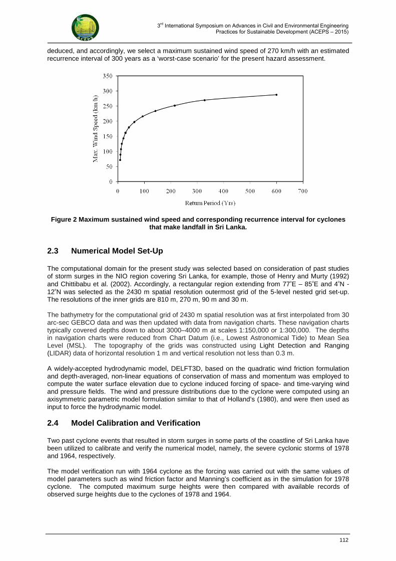
3rd International Symposium on Advances in Civil and Environmental Engineering Practices for Sustainable Development (ACEPS – 2015)
deduced, and accordingly, we select a maximum sustained wind speed of 270 km/h with an estimated recurrence interval of 300 years as a ‘worst-case scenario’ for the present hazard assessment.
Figure 2 Maximum sustained wind speed and corresponding recurrence interval for cyclones
that make landfall in Sri Lanka.
2.3 Numerical Model Set-Up The computational domain for the present study was selected based on consideration of past studies of storm surges in the NIO region covering Sri Lanka, for example, those of Henry and Murty (1992) and Chittibabu et al. (2002). Accordingly, a rectangular region extending from 77⁰E – 85⁰E and 4⁰N - 12⁰N was selected as the 2430 m spatial resolution outermost grid of the 5-level nested grid set-up. The resolutions of the inner grids are 810 m, 270 m, 90 m and 30 m. The bathymetry for the computational grid of 2430 m spatial resolution was at first interpolated from 30 arc-sec GEBCO data and was then updated with data from navigation charts. These navigation charts typically covered depths down to about 3000–4000 m at scales 1:150,000 or 1:300,000. The depths in navigation charts were reduced from Chart Datum (i.e., Lowest Astronomical Tide) to Mean Sea Level (MSL). The topography of the grids was constructed using Light Detection and Ranging (LIDAR) data of horizontal resolution 1 m and vertical resolution not less than 0.3 m. A widely-accepted hydrodynamic model, DELFT3D, based on the quadratic wind friction formulation and depth-averaged, non-linear equations of conservation of mass and momentum was employed to compute the water surface elevation due to cyclone induced forcing of space- and time-varying wind and pressure fields. The wind and pressure distributions due to the cyclone were computed using an axisymmetric parametric model formulation similar to that of Holland’s (1980), and were then used as input to force the hydrodynamic model. 2.4 Model Calibration and Verification Two past cyclone events that resulted in storm surges in some parts of the coastline of Sri Lanka have been utilized to calibrate and verify the numerical model, namely, the severe cyclonic storms of 1978 and 1964, respectively. The model verification run with 1964 cyclone as the forcing was carried out with the same values of model parameters such as wind friction factor and Manning’s coefficient as in the simulation for 1978 cyclone. The computed maximum surge heights were then compared with available records of observed surge heights due to the cyclones of 1978 and 1964.
112
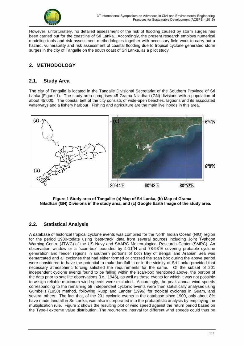
3rd International Symposium on Advances in Civil and Environmental Engineering Practices for Sustainable Development (ACEPS – 2015)
However, unfortunately, no detailed assessment of the risk of flooding caused by storm surges has been carried out for the coastline of Sri Lanka. Accordingly, the present research employs numerical modeling tools and risk assessment methodologies together with necessary field work to carry out a hazard, vulnerability and risk assessment of coastal flooding due to tropical cyclone generated storm surges in the city of Tangalle on the south coast of Sri Lanka, as a pilot study.
2. METHODOLOGY
2.1. Study Area
The city of Tangalle is located in the Tangalle Divisional Secretariat of the Southern Province of Sri Lanka (Figure 1). The study area comprises 45 Grama Niladhari (GN) divisions with a population of about 45,000. The coastal belt of the city consists of wide-open beaches, lagoons and its associated waterways and a fishery harbour. Fishing and agriculture are the main livelihoods in this area.
Figure 1 Study area of Tangalle: (a) Map of Sri Lanka, (b) Map of Grama
Niladhari (GN) Divisions in the study area, and (c) Google Earth Image of the study area.
2.2. Statistical Analysis
A database of historical tropical cyclone events was compiled for the North Indian Ocean (NIO) region for the period 1900-todate using ‘best-track’ data from several sources including Joint Typhoon Warning Centre (JTWC) of the US Navy and SAARC Meteorological Research Center (SMRC). An observation window or a ‘scan-box’ bounded by 4-11oN and 78-93oE covering probable cyclone generation and feeder regions in southern portions of both Bay of Bengal and Arabian Sea was demarcated and all cyclones that had either formed or crossed the scan box during the above period were considered to have the potential to make landfall in or in the vicinity of Sri Lanka provided that necessary atmospheric forcing satisfied the requirements for the same. Of the subset of 201 independent cyclone events found to be falling within the scan-box mentioned above, the portion of the data prior to satellite observations (i.e., 1945), as well as those events for which it was not possible to assign reliable maximum wind speeds were excluded. Accordingly, the peak annual wind speeds corresponding to the remaining 59 independent cyclonic events were then statistically analysed using Gumbel’s (1958) method, following Rupp and Lander (1996) for tropical cyclones in Guam, and several others. The fact that, of the 201 cyclonic events in the database since 1900, only about 8% have made landfall in Sri Lanka, was also incorporated into the probabilistic analysis by employing the multiplication rule. Figure 2 shows the resulting plot of wind speed against the return period based on the Type-I extreme value distribution. The recurrence interval for different wind speeds could thus be
(c)
111
3rd International Symposium on Advances in Civil and Environmental Engineering Practices for Sustainable Development (ACEPS – 2015)
Coastal Flooding Caused by Storm Surges: A Risk Assessment for the City of Tangalle in the South Coast of Sri Lanka
J. J. Wijetunge1 and C. K. Marasinghe1
1Department of Civil Engineering, University of Peradeniya,
Peradeniya 20400 SRI LANKA
E-mail: [email protected]
Abstract: Coastal flooding due to tropical cyclone generated storm surges has caused considerable damage and loss of life in the North Indian Ocean region including in Sri Lanka. This paper is concerned with an assessment of the risk of the storm surge hazard for the city of Tangalle on the south coast of Sri Lanka, as a pilot study. The present hazard assessment utilizes a database of historical events of tropical cyclones in the North Indian Ocean region. A statistical analysis of the past events has been carried out to identify an appropriate storm surge scenario. Numerical models comprising a parametric cyclone model and a hydrodynamic model based on shallow water equations have been employed to simulate cyclone wind velocity and pressure fields as well as coastal flooding due to the storm surges. The spatial distribution of the depth of inundation as well as maps of the risk to population and dwellings in the study area are presented and discussed. Keywords: Tropical cyclones, Hazard assessment, Numerical modeling, Surge height, Depth of Inundation.
1. INTRODUCTION
Sri Lanka is vulnerable to cyclones generated mostly in the southern part of Bay of Bengal, and to a lesser extent, to those in the southeast of Arabian Sea. The cyclones which form over the southernmost part of Bay of Bengal at low latitudes mainly move west or west to northwestwards into the Gulf of Mannar across the coast of Sri Lanka. These cyclones generally form during the later part of the post-monsoon season or early part of the pre-monsoon season. On the other hand, cyclones that form over Arabian Sea mostly move north or north-easterly while a few travel west or northwestwards (SAARC, 1998). However, due to atmospheric dynamics associated with cyclones and the relative proximity of Sri Lanka to the equator, a large proportion of cyclones generated in Bay of Bengal and Arabian Sea, fortunately, do not make landfall in Sri Lanka. Yet, sixteen cyclonic or severe cyclonic storms have made landfall in Sri Lanka during the last century according to the Department of Meteorology, Sri Lanka (DMSL, 2010). The loss of lives and damage and destruction to property and the environment caused by land-falling tropical cyclones could be due to some or all of the following phenomena associated with such intense weather systems, namely, extreme winds, storm surge, heavy rainfall, and sometimes, excessive rainfall leading to landslides. It must be added that, usually, much of the death toll and damage to property in coastal areas is as a result of cyclone-induced storm surge causing inundation of low-lying onshore lands (Dube, 2003; Lin et al., 2010). A storm surge is a rise above the normal water level along a shore resulting from strong onshore winds and/or reduced atmospheric pressure. The worst impact occurs when the storm surge arrives on top of a high tide. The height of the storm surge depends on cyclone dynamics such as the wind speed, the translation speed, the angle of attack at landfall, the pressure drop and also on coastal and shelf morphological factors such as the bathymetry and the shape of the coastline (Jelesnianski, 1992). Further, the severity and the extent of onshore inundation depend primarily upon the surge height and the prevailing tide as well as the elevation, the slope and the surface roughness of the terrain (Wijetunge, 2013).
110
3rd International Symposium on Advances in Civil and Environmental Engineering Practices for Sustainable Development (ACEPS – 2015)
5. ACKNOWLEDGMENTS
This study was partly funded by JSPS Asia-Africa Science Platform Program, Japan and partly by JSPS KAKENHI Grant Number 25550007, JAPAN.
6. REFERENCES
Fischer H. B. (1972). Mass transport mechanism in partially stratified estuaries. J. Fluid Mech. 53. 671-687.
Fischer H. B., List E. J., Koh R. C. Y., Imberger J. and Brooks N. H. (1979). Mixing in inland and coastal waters, Academic Press. 161.
Furusato E., Perera G. L., Tanaka N., Amarasekara G. P. and Priyadarshana, T. (2013). Current characteristics of salinity stratification of two coastal lagoons in Southern area of Sri Lanka after different human interventions. ACEPS, 231-237. Gunaratne G. L., Priyadarshana T., Manatunge J., Tanaka N. and Yasuda S. (2010b). Water balance and renewal time of Rekawa lagoon, Sri Lanka; A restorative approach. International Conference on Sustainable Built Environment (ICSBE-2010). 37-44.
Gunaratne G. L., Tanaka N., Amarasekara., P. Priyadarshana T. and Manatunge J. (2010a). Restoration of Koggala lagoon: Modelling approach in evaluating lagoon water budget and flow characteristics. Journal of environmental sciences. 22(6).813-819.
Hansen D. V. and Rattray M. (1966). New dimensions in estuary classification. Limnol. Oceanogr. 11, 319-325.
IUCN (2006). Sri Lanka and the Central Environmental Authority, National wetland directory of Sri Lanka, Colombo, Sri Lanka.123.
Kjerfve B. and Magill K., E. (1989). Geographic and hydrodynamic characteristics of shallow coastal lagoons. Marine Geology. 8.187-199.
McCutcheon S. C., Martin J. L. and Barnwell T. O. Jr. Water Quality. in Maidment, D. R. (Editor)(1993). Handbook of Hydrology. McGraw-Hill, New York, NY.11.3.
Perera G.L., Furusato E. and Priyadarshana T. (2015). A Simple Bulk Model to Estimate Salinity Stratification of Permanently Open Choked Coastal Lagoons in Sri Lanka. Annual Journal of Hydraulic Engineering. JSCE, 71, accepted.
Pritchard W. D. (1955), Estuarine circulation patterns. Proc. Am. Soc. Civil Eng. 81(717).1-11
Priyadarshana T, Aseada T. (2006), Impact on Ecohydrology of Rekewa Lagoon in Southern Sri Lanka and its Restoration Efforts. Asia Oceania Geosciences Society (AOGS), Singapore, 2006
Priyadarshana T., Manatunge J. and Wijeratne N. (2007). Impacts and consequences of removal of the sand bar at the Koggala lagoon mouth and rehabilitation of the lagoon mouth to restore natural formation of the sand bar. Report, Practical Action, Sri Lanka.
Rekawa special area management coordinating committee (1996), Special area management plan for Rekawa Lagoon, Sri Lanka, Coastal resources management project of the University of Rhode Island and the United States Agency for International Development.
Simpson H. J., Brown J., Matthews J. and Allen G.(1990). Tidal straining density currents and stirring in the control of estuarine stratification. Eistuaries. 13. No2.125-132.
109
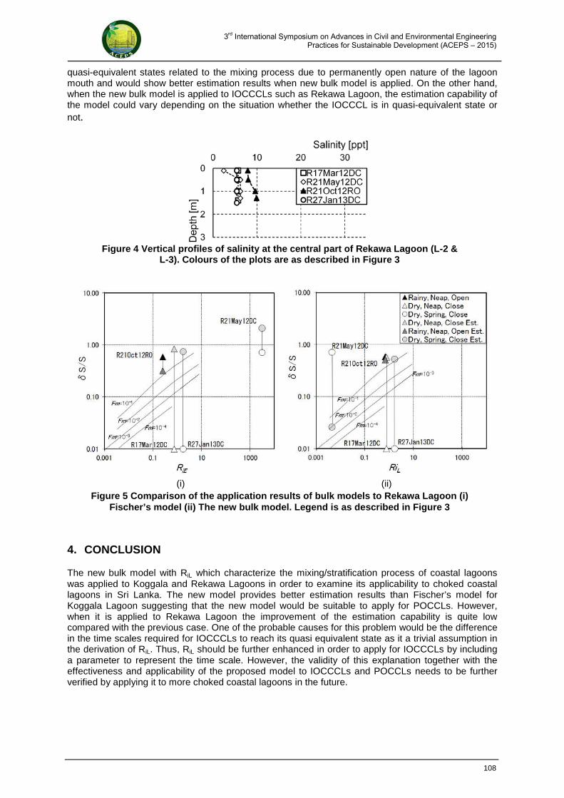
3rd International Symposium on Advances in Civil and Environmental Engineering Practices for Sustainable Development (ACEPS – 2015)
quasi-equivalent states related to the mixing process due to permanently open nature of the lagoon mouth and would show better estimation results when new bulk model is applied. On the other hand, when the new bulk model is applied to IOCCCLs such as Rekawa Lagoon, the estimation capability of the model could vary depending on the situation whether the IOCCCL is in quasi-equivalent state or not.
4. CONCLUSION
The new bulk model with RiL which characterize the mixing/stratification process of coastal lagoons was applied to Koggala and Rekawa Lagoons in order to examine its applicability to choked coastal lagoons in Sri Lanka. The new model provides better estimation results than Fischer’s model for Koggala Lagoon suggesting that the new model would be suitable to apply for POCCLs. However, when it is applied to Rekawa Lagoon the improvement of the estimation capability is quite low compared with the previous case. One of the probable causes for this problem would be the difference in the time scales required for IOCCCLs to reach its quasi equivalent state as it a trivial assumption in the derivation of RiL. Thus, RiL should be further enhanced in order to apply for IOCCCLs by including a parameter to represent the time scale. However, the validity of this explanation together with the effectiveness and applicability of the proposed model to IOCCCLs and POCCLs needs to be further verified by applying it to more choked coastal lagoons in the future.
Figure 4 Vertical profiles of salinity at the central part of Rekawa Lagoon (L-2 &
L-3). Colours of the plots are as described in Figure 3
(i) (ii)
Figure 5 Comparison of the application results of bulk models to Rekawa Lagoon (i) Fischer’s model (ii) The new bulk model. Legend is as described in Figure 3
108
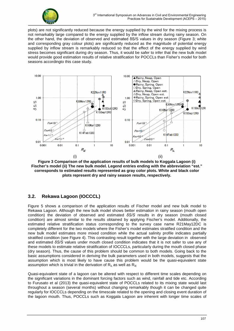
3rd International Symposium on Advances in Civil and Environmental Engineering Practices for Sustainable Development (ACEPS – 2015)
plots) are not significantly reduced because the energy supplied by the wind for the mixing process is not remarkably large compared to the energy supplied by the inflow stream during rainy season. On the other hand, the deviation of observed and estimated δS/S values in dry season (Figure 3; white and corresponding gray colour plots) are significantly reduced as the magnitude of potential energy supplied by inflow stream is remarkably reduced so that the effect of the energy supplied by wind stress becomes significant during dry season. Thus, it would be safer to infer that the new bulk model would provide good estimation results of relative stratification for POCCLs than Fisher’s model for both seasons accordingto this case study.
3.2. Rekawa Lagoon (IOCCCL)
Figure 5 shows a comparison of the application results of Fischer model and new bulk model to Rekawa Lagoon. Although the new bulk model shows better estimation in rainy season (mouth open condition) the deviation of observed and estimated δS/S results in dry season (mouth closed condition) are almost similar to the results obtained by applying Fischer’s model. Additionally, the estimated relative stratification status corresponding to the survey case name R21May12DC is completely different for the two models where the Fisher’s model estimates stratified condition and the new bulk model estimates more mixed condition while the actual salinity profile indicates partially stratified condition (see Figure 4). This contrasting result together with the large deviation in observed and estimated δS/S values under mouth closed condition indicates that it is not safer to use any of these models to estimate relative stratification of IOCCCLs, particularly during the mouth closed phase (dry season). Thus, the cause of this problem should be common to both models. Going back to the basic assumptions considered in deriving the bulk parameters used in both models, suggests that the assumption which is most likely to have cause this problem would be the quasi-equivalent state assumption which is trivial in the derivation of RiL as well as RiE Quasi-equivalent state of a lagoon can be altered with respect to different time scales depending on the significant variations in the dominant forcing factors such as wind, rainfall and tide etc. According to Furusato et al (2013) the quasi-equivalent state of POCCLs related to its mixing state would last throughout a season (several months) without changing remarkably though it can be changed quite regularly for IOCCCLs depending on the timescale related to the opening and closing event duration of the lagoon mouth. Thus, POCCLs such as Koggala Lagoon are inherent with longer time scales of
(i) (ii)
Figure 3 Comparison of the application results of bulk models to Koggala Lagoon (i) Fischer’s model (ii) The new bulk model. Legend entries ending with the abbreviation “est.”
corresponds to estimated results represented as gray color plots. White and black color plots represent dry and rainy season results, respectively.
107
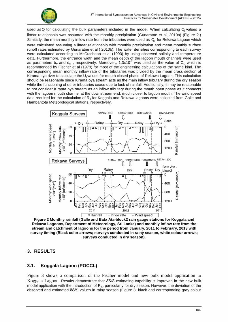
3rd International Symposium on Advances in Civil and Environmental Engineering Practices for Sustainable Development (ACEPS – 2015)
used as IQ for calculating the bulk parameters included in the model. When calculating IQ values a linear relationship was assumed with the monthly precipitation (Gunaratne et al, 2010a) (Figure 2.) Similarly, the mean monthly inflow rate from the tributaries were used as IQ for Rekawa Lagoon which were calculated assuming a linear relationship with monthly precipitation and mean monthly surface runoff rates estimated by Gunaratne et al ( 2010b). The water densities corresponding to each survey were calculated according to McCutcheon et al (1993) by using observed salinity and temperature data. Furthermore, the entrance width and the mean depth of the lagoon mouth channels were used as parameters bM and dM , respectively. Moreover,, 1.3x10⁻³ was used as the value of CD which is recommended by Fischer et al (1979) for most of the engineering calculations of the same kind. The corresponding mean monthly inflow rate of the tributaries was divided by the mean cross section of Kirama oya river to calculate the Ut values for mouth closed phase of Rekawa Lagoon. This calculation should be reasonable since Kirama oya stream acts as the main inflow tributary during the dry season while the functioning of other tributaries cease due to lack of rainfall. Additionally, it may be reasonable to not consider Kirama oya stream as an inflow tributary during the mouth open phase as it connects with the lagoon mouth channel at the downstream end, much closer to lagoon mouth. The wind speed data required for the calculation of RiL for Koggala and Rekawa lagoons were collected from Galle and Hambantota Meteorological stations, respectively.
Figure 2 Monthly rainfall (Galle and Bata Ata-block2 rain gauge stations for Koggala and
Rekawa Lagoons, Department of Meteorology, Sri Lanka) and monthly inflow rate from the stream and catchment of lagoons for the period from January, 2011 to February, 2013 with
survey timing (Black color arrows; surveys conducted in rainy season, white colour arrows; surveys conducted in dry season).
3. RESULTS
3.1. Koggala Lagoon (POCCL)
Figure 3 shows a comparison of the Fischer model and new bulk model application to Koggala Lagoon. Results demonstrate that δS/S estimating capability is improved in the new bulk model application with the introduction of RiL, particularly for dry season. However, the deviation of the observed and estimated δS/S values in rainy season (Figure 3; black and corresponding gray colour
106
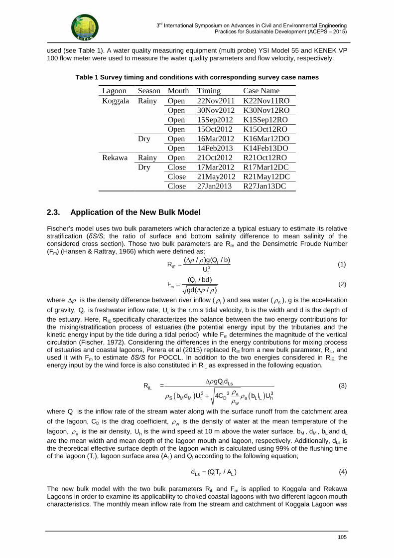
3rd International Symposium on Advances in Civil and Environmental Engineering Practices for Sustainable Development (ACEPS – 2015)
used (see Table 1). A water quality measuring equipment (multi probe) YSI Model 55 and KENEK VP 100 flow meter were used to measure the water quality parameters and flow velocity, respectively.
Table 1 Survey timing and conditions with corresponding survey case names
Lagoon Season Mouth Timing Case Name Koggala Rainy Open 22Nov2011 K22Nov11RO
Open 30Nov2012 K30Nov12RO Open 15Sep2012 K15Sep12RO Open 15Oct2012 K15Oct12RO
Dry Open 16Mar2012 K16Mar12DO Open 14Feb2013 K14Feb13DO
Rekawa Rainy Open 21Oct2012 R21Oct12RO Dry Close 17Mar2012 R17Mar12DC
Close 21May2012 R21May12DC Close 27Jan2013 R27Jan13DC
2.3. Application of the New Bulk Model
Fischer’s model uses two bulk parameters which characterize a typical estuary to estimate its relative stratification (δS/S; the ratio of surface and bottom salinity difference to mean salinity of the considered cross section). Those two bulk parameters are RiE and the Densimetric Froude Number (Fm) (Hansen & Rattray, 1966) which were defined as;
ρ ρ∆= 3
( / ) ( / )fiE
t
g Q bR
U (1)
ρ ρ=
∆( / )
( / )f
m
Q bdF
gd (2)
where ρ∆ is the density difference between river inflow ( ρI ) and sea water ( ρS ), g is the acceleration
of gravity, fQ is freshwater inflow rate, tU is the r.m.s tidal velocity, b is the width and d is the depth of the estuary. Here, RiE specifically characterizes the balance between the two energy contributions for the mixing/stratification process of estuaries (the potential energy input by the tributaries and the kinetic energy input by the tide during a tidal period) while Fm determines the magnitude of the vertical circulation (Fischer, 1972). Considering the differences in the energy contributions for mixing process of estuaries and coastal lagoons, Perera et al (2015) replaced RiE from a new bulk parameter, RiL, and used it with Fm to estimate δS/S for POCCL. In addition to the two energies considered in RiE, the energy input by the wind force is also constituted in RiL as expressed in the following equation.
( ) ( )
ρρρ ρρ
∆
+3 3 3
=
4
I LsiL
aS M M t D a L L h
w
gQ dR
b d U C b l U
(3)
where IQ is the inflow rate of the stream water along with the surface runoff from the catchment area
of the lagoon, CD is the drag coefficient, ρw is the density of water at the mean temperature of the
lagoon, aρ is the air density, hU is the wind speed at 10 m above the water surface. bM , dM , bL and dL
are the mean width and mean depth of the lagoon mouth and lagoon, respectively. Additionally, dLs is the theoretical effective surface depth of the lagoon which is calculated using 99% of the flushing time of the lagoon (Tr), lagoon surface area (AL) and QI according to the following equation;
= ( / )Ls I r Ld QT A (4)
The new bulk model with the two bulk parameters RiL and Fm is applied to Koggala and Rekawa Lagoons in order to examine its applicability to choked coastal lagoons with two different lagoon mouth characteristics. The monthly mean inflow rate from the stream and catchment of Koggala Lagoon was
105
3rd International Symposium on Advances in Civil and Environmental Engineering Practices for Sustainable Development (ACEPS – 2015)
2.1.1. Koggala Lagoon
Koggala Lagoon (5°58’ 6° 20’ N and 80°17’ 80°22’ E) is situated about130 km south from the country’s trade capital, Colombo. Prior to 1995, Koggala Lagoon was an IOCCCL with a freshwater ecosystem. Recent anthropogenic activities such as unplanned sand removal and structural intervention at the lagoon mouth area turned Koggala Lagoon to a POCCL, consequently shifting its ecosystem towards more saline conditions. This transformation has generated various environmental and socio-economic problems (Priyadarshana et al, 2007). Having a waterway area of 7.27 km2, Koggala Lagoon is approximately 4.8 km long and 2 km wide. The hydro-catchment area of Koggala Lagoon is approximately 55 km2 consisting mainly homesteads and cultivated fields of paddy, coconut, tea, rubber and other plantations (Priyadarshana et al, 2007). The depth of the lagoon ranges from 1.0 to 3.7 m and it can vary according to seasonal changes in rainfall. Koggala Lagoon usually experiences a mean annual rainfall of between 2,000 and 2, 500 mm (IUCN, 2006). Although it receives freshwater influx from several streams, more than 88% of the stream water is received to the lagoon through Warabokka stream. Lagoon’s main water body is enclosed with 14 islets and the largest one is located in the south east corner of the lagoon. Lagoon mouth channel that connects the lagoon with the sea is located at the south east corner. Two bridges that was built as a part of the Colombo-Matara main road and rail track lie across the lagoon mouth channel of which the approximate width closer to rail track bridge is about 100 m.
2.1.2. Rekawa Lagoon
Rekawa Lagoon (50° 58’N and 80° 47E) is situated about 200 km south from the country’s trade capital, Colombo. The hydro-catchment area of Rekawa Lagoon is approximately 225 km2 consisting of a large tract of paddy fields, mangrove and scrub forest and homestead (Rekawa special area management coordinating committee, 1996). Lagoon’s surface extends up to approximately 1 km in width at the widest point and about 3.3 km in length along the shoreline, claiming to a surface area of 2.38 km2 (Priyadarshana & Aseada, 2006). Kirama oya stream which connects with the lagoon mouth channel 0.7 km from the sea has been the main inflow tributary of the lagoon, especially during the mouth closed phase of the lagoon. Additionally, the lagoon receives freshwater from another inflow tributary which connects at downstream end of the lagoon’s main water body from the landward side and operates mostly in rainy season. This significant positioning of inflow tributaries together with relatively deep 2 km long meandering lagoon mouth channel makes Rekawa Lagoon a unique coastal water body. Although Rekawa Lagoon claims to a relatively larger catchment area, the numerous irrigation structures constructed along the inflow tributaries of Rekawa Lagoon has been significantly reducing the freshwater flow into the lagoon (Rekawa special area management coordinating committee, 1996). Rekawa Lagoon mouth is periodically closed, especially in dry season, as the winds and constant waves on the shoreline give rise to dispositional sand dunes along the coast and occasionally opened in rainy season naturally or artificially by local community to prevent flooding when higher amount of rainfall is received to the catchment area. The water depth of the lagoon can vary depending on the seasonal variations in rainfall as well as the open or close state of the lagoon mouth. Kapuhenwala causeway constructed across the lagoon mouth channel in 1984 has been drastically altering the natural rhythm of the lagoon as it impedes the water circulation of the lagoon (Rekawa special area management coordinating committee, 1996).
2.2. Field Observations
Field observations were conducted to investigate salinity stratification characteristics of the two lagoons during the time period starting from November 2011 to February 2013 under different seasonal, tidal and mouth conditions (Table 1). Vertical profiles of salinity, dissolved oxygen, water temperature and flow velocity were measured with 0.5 m vertical intervals at several points covering all the key parts of the lagoons, lagoon mouths, main water bodies and main inflow tributaries. However in this study, the data collected at the selected main representative survey point of the central parts of the lagoons are presented. The selected survey point to represent the central part of Koggala Lagoon was L-1 while it was L-2 for all the cases of Rekawa Lagoon, except for the case named R21May12DC where the data collected at L-3 point was
104
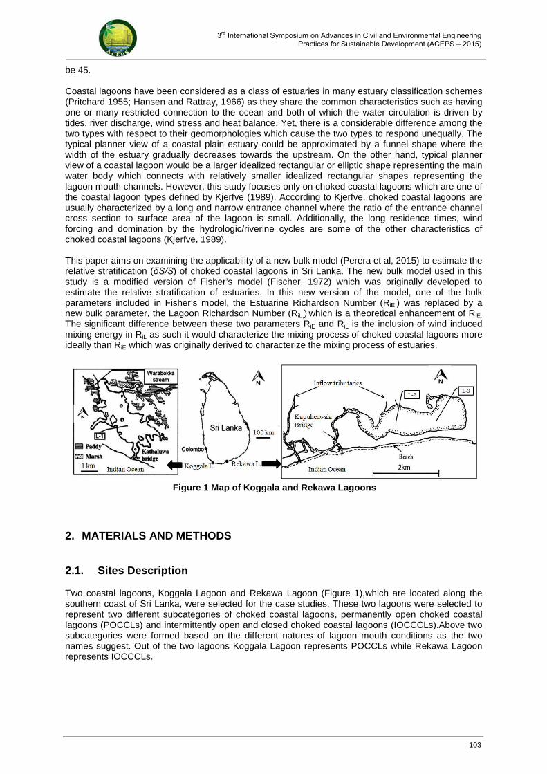
3rd International Symposium on Advances in Civil and Environmental Engineering Practices for Sustainable Development (ACEPS – 2015)
be 45. Coastal lagoons have been considered as a class of estuaries in many estuary classification schemes (Pritchard 1955; Hansen and Rattray, 1966) as they share the common characteristics such as having one or many restricted connection to the ocean and both of which the water circulation is driven by tides, river discharge, wind stress and heat balance. Yet, there is a considerable difference among the two types with respect to their geomorphologies which cause the two types to respond unequally. The typical planner view of a coastal plain estuary could be approximated by a funnel shape where the width of the estuary gradually decreases towards the upstream. On the other hand, typical planner view of a coastal lagoon would be a larger idealized rectangular or elliptic shape representing the main water body which connects with relatively smaller idealized rectangular shapes representing the lagoon mouth channels. However, this study focuses only on choked coastal lagoons which are one of the coastal lagoon types defined by Kjerfve (1989). According to Kjerfve, choked coastal lagoons are usually characterized by a long and narrow entrance channel where the ratio of the entrance channel cross section to surface area of the lagoon is small. Additionally, the long residence times, wind forcing and domination by the hydrologic/riverine cycles are some of the other characteristics of choked coastal lagoons (Kjerfve, 1989). This paper aims on examining the applicability of a new bulk model (Perera et al, 2015) to estimate the relative stratification (δS/S) of choked coastal lagoons in Sri Lanka. The new bulk model used in this study is a modified version of Fisher’s model (Fischer, 1972) which was originally developed to estimate the relative stratification of estuaries. In this new version of the model, one of the bulk parameters included in Fisher’s model, the Estuarine Richardson Number (RiE,) was replaced by a new bulk parameter, the Lagoon Richardson Number (RiL,) which is a theoretical enhancement of RiE.
The significant difference between these two parameters RiE and RiL is the inclusion of wind induced mixing energy in RiL as such it would characterize the mixing process of choked coastal lagoons more ideally than RiE which was originally derived to characterize the mixing process of estuaries.
2. MATERIALS AND METHODS
2.1. Sites Description
Two coastal lagoons, Koggala Lagoon and Rekawa Lagoon (Figure 1),which are located along the southern coast of Sri Lanka, were selected for the case studies. These two lagoons were selected to represent two different subcategories of choked coastal lagoons, permanently open choked coastal lagoons (POCCLs) and intermittently open and closed choked coastal lagoons (IOCCCLs).Above two subcategories were formed based on the different natures of lagoon mouth conditions as the two names suggest. Out of the two lagoons Koggala Lagoon represents POCCLs while Rekawa Lagoon represents IOCCCLs.
Figure 1 Map of Koggala and Rekawa Lagoons
103
3rd International Symposium on Advances in Civil and Environmental Engineering Practices for Sustainable Development (ACEPS – 2015)
Applicability of Salinity Stratification Estimation by New Bulk Model for Two Choked Coastal Lagoons in Sri Lanka
G. L. Perera1, E. Furusato1,2 , G. P. Amarasekara3 and T. Priyadarshana3
1Graduate School of Science and Engineering, Saitama University
255 Shimo-Okubo, Sakura-ku, Saitama 338-8570 JAPAN
2 International Institute for Resilient Society,
Saitama University 255 Shimo-Okubo, Sakura-ku, Saitama 338-8570
JAPAN
3 Faculty of Fisheries and Marine Sciences & Technology, University of Ruhuna
Wellamadama, Matara (81000), Sri Lanka
E-mail: [email protected]
Abstract: Two coastal lagoons in Sri Lanka, Koggala and Rekawa were studied to examine the applicability of a new bulk model to estimate relative stratification of choked lagoons. Two lagoons selected for the study represent two subcategories of choked coastal lagoons; permanently open choked coastal lagoons (POCCLs) and intermittently open and closed choked coastal lagoons (IOCCCLs). Application results for Koggala Lagoon demonstrate that δS/S estimation capability of the new bulk model is superior to Fischer’s model, suggesting that the new bulk model would be suitable to apply for POCCLs. On the other hand, when the model was applied to Rekawa Lagoon, it demonstrated poor δS/S estimation capability compared to the POCCL case. This might have caused due to the variation in the time scale required for the IOCCCLs to reach the quasi equivalent state related to mixing process as the quasi equivalent state assumption is trivial in RiL derivation. Keywords: Coastal lagoons, salinity stratification, Estuarine Richardson Number, wind induced mixing, Lagoon Richardson Number, Quasi-equivalent state
1. INTRODUCTION
Sustainable use of coastal lagoons in Sri Lanka is becoming essential as the lagoon environments are being rapidly and indiscriminately exploited by anthropogenic activities over the recent decade (IUCN, 2006). A comprehensive knowledge on the various aspects of coastal lagoons, including their physical process is a prerequisite for their sustainable use while preserving their naturalness. One such important physical process is the vertical mixing/stratification process and the level of stratification of coastal lagoons due to saline water intrusion. These can be crucial in determining the changes on the inherent nature of coastal lagoons as the vertical fluxes of water properties such as dissolved oxygen and nutrient elements depend on them (Simpson et al, 1990). Simple bulk models could be useful for estimating the degree of stratification of coastal lagoons as they can be easily applied with minimum field requirements, unlike numerical models. These models become more useful in situations where there are no proper systems to monitor large number of hydrologic/riverine parameters on a regular basis, such as what is commonly experienced in coastal lagoons in Sri Lanka. Despite the controversies over the identification of coastal lagoons from estuaries, the number of coastal lagoons situated along the entire coast of Sri Lanka is estimated to
102
3rd International Symposium on Advances in Civil and Environmental Engineering Practices for Sustainable Development (ACEPS – 2015)
Costal and Lagoon Environment
101

3rd International Symposium on Advances in Civil and Environmental Engineering Practices for Sustainable Development (ACEPS – 2015)
Xu, B., Low, B.K. and Asce, F., (2006). Probabilistic Stability Analyses of Embankments Based on Finite-Element Method. Journal of geotechnical and geoenvironmental engineering ASCE, November, 2006, pp.1444–1454. Zekkos, D., George, A. A., Jonathan, D. B., Athena, G., Andreas, T., (2010). Large-scale direct shear testing of municipal solid waste. Waste management (New York, N.Y.), 30(8-9), pp.1544–55. Zhan, T.L.T., Chen, Y.M. and Ling, W.A., (2008). Shear strength characterization of municipal solid waste at the Suzhou landfill, China. Engineering Geology, 97(3-4), pp.97–111.
100
3rd International Symposium on Advances in Civil and Environmental Engineering Practices for Sustainable Development (ACEPS – 2015)
5. SUMMARY AND CONCLUSIONS
Based on the laboratory experiments and the results obtained from FEM analysis, following conclusions can be drawn;
• Shear strength parameters showed erratic behaviour for samples tested while direct shear test results proved to be very high. The reason behind such high cohesion and friction angle values can be explained by the fact that solid waste tested had a high content (about 60% by dry mass) of fine particles (<4.75 mm) and gravel (about 20% by dry mass)
• Slope stability of MSW landfills must be evaluated by adopting a probabilistic approach. Conventional FOS methods only consider a single set of input data when producing a factor of safety for a slope. Thus, variation in shear strength parameters of the waste layer and uncertainties involved in conducting tests are not accounted for. By using the reliability analysis via response surface method, the uncertainties involved with the spatial distribution of landfilled MSW shear strength parameters can be accounted for. The proposed model can be easily adopted in evaluation of slope stability of MSW landfills in the country and is compatible with various deterministic stability methods (both finite element modelling and limit equilibrium method) with readily available software without the need for additional coding.
• The method can be extended for analysis in the wet zone of the country incorporating pore water pressure within the waste mass as another random variable, enabling the evaluation of stability of a solid waste slope under saturated conditions. This will further increase the number of sample points required to determine the performance function for the factor of safety. It is recommended to conduct testing for waste samples with larger particle sizes depending on the average particle size of the waste body to obtain more accurate shear strength parameters as input variables.
6. ACKNOWLEDGMENTS
This is one of the projects funded under the project ‘Development of Pollution Control and Environmental Restoration Technologies of Waste Landfill Sites Taking into Account Geographical Characteristics in Sri Lanka’, of Science and Technology Research Partnership for Sustainable Development (SATREPS) and the Authors would like to acknowledge the financial aid given JICA. The Facilities provided by University of Ruhuna to conduct the research study is also acknowledged.
7. REFERENCES
Cañizal, J., Lapeña, P., Castro, J., Da Costa, A., and Sagaseta, C., (2011). Determination of shear strength of MSW. Field tests versus Laboratory tests. Paper presented at the Fourth International Workshop Hydro-Physico-Mechanics of Landfills. Gibson, W., (2011). Probabilistic methods for slope analysis and design, Australian Geomechanics vol 46. No. 3 Hoornweg, D., Bhada-Tata, P., and Peterson, C., (2013), ‘World Bank Review of Solid Waste Management’. 20 February 2013 Jafari, N.H., Stark, T.D., & Merry, S., (2013). The July 10 2000 Payatas Landfill Slope Failure. International Journal of Geoengineering Case Histories, 2(3), pp.208–228 Low, B.K., (1996). Practical probabilistic approach using spreadsheet. ASCE Geotechnical Special Publication No. 58, Proc., Uncertainty in the Geologic Environment – From theory to Practis, Masixon, Wisconsin, July 31- August 3, Vol. 2, pp.1284-1302 Reddy, K.R., Hettiarachchi, H.P., Naveen, S.G., Janardhanan, B,. Jean, E., (2009). ‘Compressibility and shear strength of municipal solid waste under short-term leachate recirculation operations’. Waste management and research : The journal of the International Solid Wastes and Public Cleansing Association, ISWA, 27(6), pp.578–87.
99
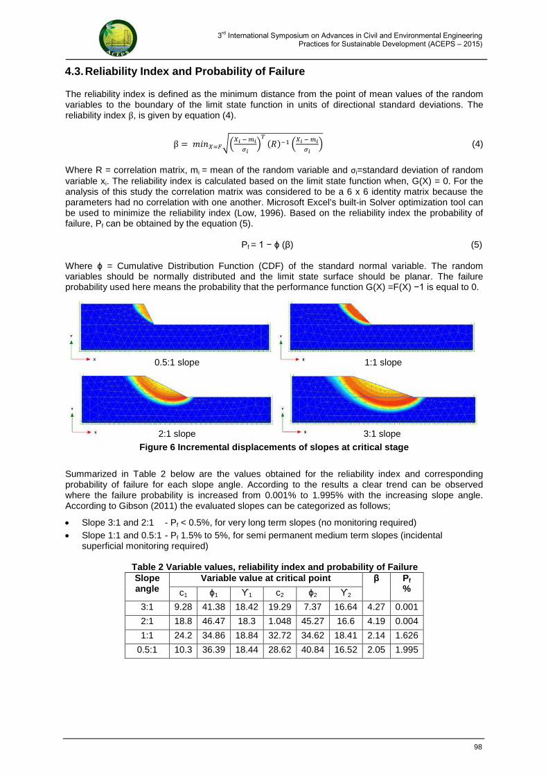
3rd International Symposium on Advances in Civil and Environmental Engineering Practices for Sustainable Development (ACEPS – 2015)
4.3. Reliability Index and Probability of Failure
The reliability index is defined as the minimum distance from the point of mean values of the random variables to the boundary of the limit state function in units of directional standard deviations. The reliability index β, is given by equation (4).
β = 𝑚𝑚𝑚𝑚𝑛𝑛𝑋𝑋=𝐹𝐹��𝑋𝑋𝑖𝑖 − 𝑚𝑚𝑖𝑖
𝜎𝜎𝑖𝑖�𝑇𝑇
(𝑅𝑅)−1 �𝑋𝑋𝑖𝑖 − 𝑚𝑚𝑖𝑖𝜎𝜎𝑖𝑖
� (4)
Where R = correlation matrix, mi = mean of the random variable and σi=standard deviation of random variable xi. The reliability index is calculated based on the limit state function when, G(X) = 0. For the analysis of this study the correlation matrix was considered to be a 6 x 6 identity matrix because the parameters had no correlation with one another. Microsoft Excel’s built-in Solver optimization tool can be used to minimize the reliability index (Low, 1996). Based on the reliability index the probability of failure, Pf can be obtained by the equation (5).
Pf = 1 − ɸ (β) (5)
Where ɸ = Cumulative Distribution Function (CDF) of the standard normal variable. The random variables should be normally distributed and the limit state surface should be planar. The failure probability used here means the probability that the performance function G(X) =F(X) −1 is equal to 0.
Figure 6 Incremental displacements of slopes at critical stage
Summarized in Table 2 below are the values obtained for the reliability index and corresponding probability of failure for each slope angle. According to the results a clear trend can be observed where the failure probability is increased from 0.001% to 1.995% with the increasing slope angle. According to Gibson (2011) the evaluated slopes can be categorized as follows;
• Slope 3:1 and 2:1 - Pf < 0.5%, for very long term slopes (no monitoring required) • Slope 1:1 and 0.5:1 - Pf 1.5% to 5%, for semi permanent medium term slopes (incidental
superficial monitoring required)
Table 2 Variable values, reliability index and probability of Failure Slope angle
Variable value at critical point β Pf
% c1 ɸ1 ϒ1 c2 ɸ2 ϒ2
3:1 9.28 41.38 18.42 19.29 7.37 16.64 4.27 0.001
2:1 18.8 46.47 18.3 1.048 45.27 16.6 4.19 0.004
1:1 24.2 34.86 18.84 32.72 34.62 18.41 2.14 1.626
0.5:1 10.3 36.39 18.44 28.62 40.84 16.52 2.05 1.995
0.5:1 slope 1:1 slope
2:1 slope 3:1 slope
98
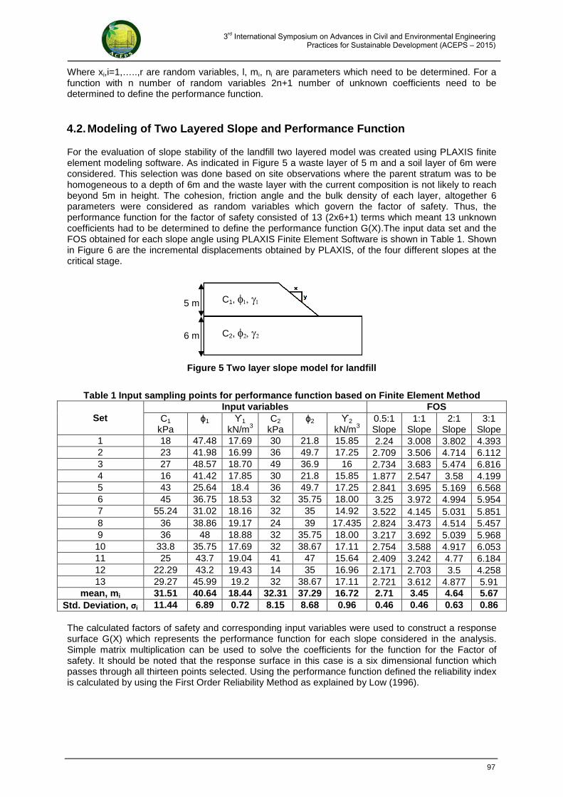
3rd International Symposium on Advances in Civil and Environmental Engineering Practices for Sustainable Development (ACEPS – 2015)
Where xi,i=1,…..,r are random variables, l, mi, ni are parameters which need to be determined. For a function with n number of random variables 2n+1 number of unknown coefficients need to be determined to define the performance function.
4.2. Modeling of Two Layered Slope and Performance Function
For the evaluation of slope stability of the landfill two layered model was created using PLAXIS finite element modeling software. As indicated in Figure 5 a waste layer of 5 m and a soil layer of 6m were considered. This selection was done based on site observations where the parent stratum was to be homogeneous to a depth of 6m and the waste layer with the current composition is not likely to reach beyond 5m in height. The cohesion, friction angle and the bulk density of each layer, altogether 6 parameters were considered as random variables which govern the factor of safety. Thus, the performance function for the factor of safety consisted of 13 (2x6+1) terms which meant 13 unknown coefficients had to be determined to define the performance function G(X).The input data set and the FOS obtained for each slope angle using PLAXIS Finite Element Software is shown in Table 1. Shown in Figure 6 are the incremental displacements obtained by PLAXIS, of the four different slopes at the critical stage.
Figure 5 Two layer slope model for landfill
Table 1 Input sampling points for performance function based on Finite Element Method
Set Input variables FOS
C1
kPa ɸ1 ϒ1
kN/m3 C2
kPa ɸ2 ϒ2
kN/m3 0.5:1 Slope
1:1 Slope
2:1 Slope
3:1 Slope
1 18 47.48 17.69 30 21.8 15.85 2.24 3.008 3.802 4.393 2 23 41.98 16.99 36 49.7 17.25 2.709 3.506 4.714 6.112 3 27 48.57 18.70 49 36.9 16 2.734 3.683 5.474 6.816 4 16 41.42 17.85 30 21.8 15.85 1.877 2.547 3.58 4.199 5 43 25.64 18.4 36 49.7 17.25 2.841 3.695 5.169 6.568 6 45 36.75 18.53 32 35.75 18.00 3.25 3.972 4.994 5.954 7 55.24 31.02 18.16 32 35 14.92 3.522 4.145 5.031 5.851 8 36 38.86 19.17 24 39 17.435 2.824 3.473 4.514 5.457 9 36 48 18.88 32 35.75 18.00 3.217 3.692 5.039 5.968 10 33.8 35.75 17.69 32 38.67 17.11 2.754 3.588 4.917 6.053 11 25 43.7 19.04 41 47 15.64 2.409 3.242 4.77 6.184 12 22.29 43.2 19.43 14 35 16.96 2.171 2.703 3.5 4.258 13 29.27 45.99 19.2 32 38.67 17.11 2.721 3.612 4.877 5.91
mean, mi 31.51 40.64 18.44 32.31 37.29 16.72 2.71 3.45 4.64 5.67 Std. Deviation, σi 11.44 6.89 0.72 8.15 8.68 0.96 0.46 0.46 0.63 0.86
The calculated factors of safety and corresponding input variables were used to construct a response surface G(X) which represents the performance function for each slope considered in the analysis. Simple matrix multiplication can be used to solve the coefficients for the function for the Factor of safety. It should be noted that the response surface in this case is a six dimensional function which passes through all thirteen points selected. Using the performance function defined the reliability index is calculated by using the First Order Reliability Method as explained by Low (1996).
5 m 6 m
C1, φ1, γ1
C2, φ2, γ2
97
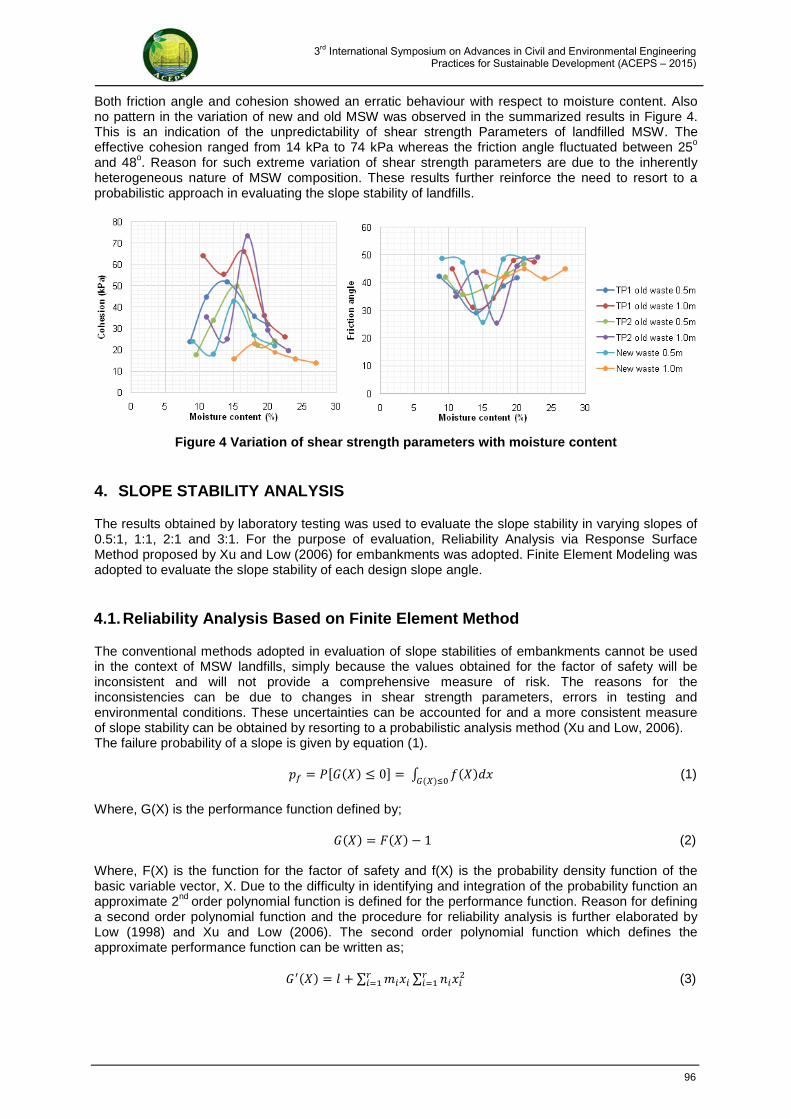
3rd International Symposium on Advances in Civil and Environmental Engineering Practices for Sustainable Development (ACEPS – 2015)
Both friction angle and cohesion showed an erratic behaviour with respect to moisture content. Also no pattern in the variation of new and old MSW was observed in the summarized results in Figure 4. This is an indication of the unpredictability of shear strength Parameters of landfilled MSW. The effective cohesion ranged from 14 kPa to 74 kPa whereas the friction angle fluctuated between 25o and 48o. Reason for such extreme variation of shear strength parameters are due to the inherently heterogeneous nature of MSW composition. These results further reinforce the need to resort to a probabilistic approach in evaluating the slope stability of landfills.
Figure 4 Variation of shear strength parameters with moisture content
4. SLOPE STABILITY ANALYSIS
The results obtained by laboratory testing was used to evaluate the slope stability in varying slopes of 0.5:1, 1:1, 2:1 and 3:1. For the purpose of evaluation, Reliability Analysis via Response Surface Method proposed by Xu and Low (2006) for embankments was adopted. Finite Element Modeling was adopted to evaluate the slope stability of each design slope angle.
4.1. Reliability Analysis Based on Finite Element Method
The conventional methods adopted in evaluation of slope stabilities of embankments cannot be used in the context of MSW landfills, simply because the values obtained for the factor of safety will be inconsistent and will not provide a comprehensive measure of risk. The reasons for the inconsistencies can be due to changes in shear strength parameters, errors in testing and environmental conditions. These uncertainties can be accounted for and a more consistent measure of slope stability can be obtained by resorting to a probabilistic analysis method (Xu and Low, 2006). The failure probability of a slope is given by equation (1). 𝑝𝑝𝑓𝑓 = 𝑃𝑃[𝐺𝐺(𝑋𝑋) ≤ 0] = ∫ 𝑓𝑓(𝑋𝑋)𝑑𝑑𝑑𝑑
𝐺𝐺(𝑋𝑋)≤0 (1)
Where, G(X) is the performance function defined by; 𝐺𝐺(𝑋𝑋) = 𝐹𝐹(𝑋𝑋) − 1 (2) Where, F(X) is the function for the factor of safety and f(X) is the probability density function of the basic variable vector, X. Due to the difficulty in identifying and integration of the probability function an approximate 2nd order polynomial function is defined for the performance function. Reason for defining a second order polynomial function and the procedure for reliability analysis is further elaborated by Low (1998) and Xu and Low (2006). The second order polynomial function which defines the approximate performance function can be written as; 𝐺𝐺′(𝑋𝑋) = 𝑙𝑙 + ∑ 𝑚𝑚𝑖𝑖𝑑𝑑𝑖𝑖𝑟𝑟
𝑖𝑖=1 ∑ 𝑛𝑛𝑖𝑖𝑑𝑑𝑖𝑖2𝑟𝑟𝑖𝑖=1 (3)
96
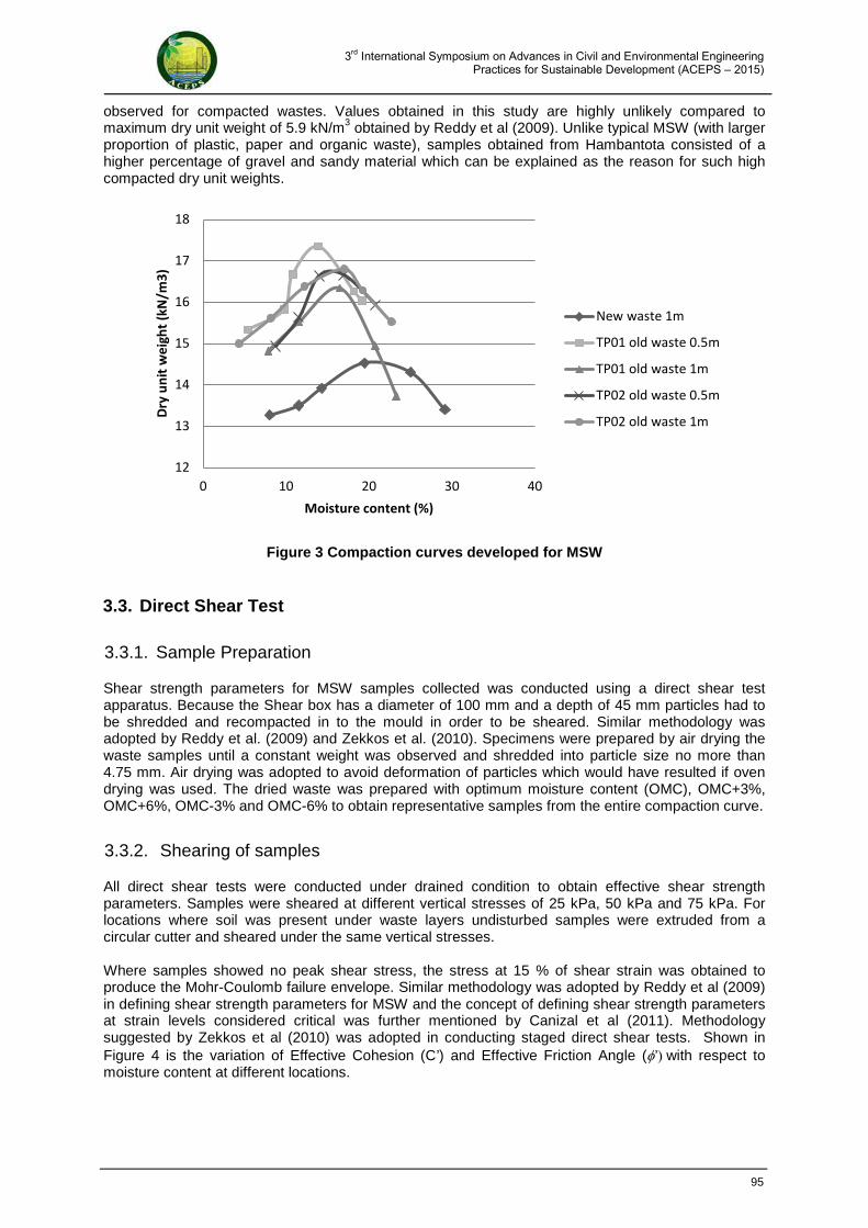
3rd International Symposium on Advances in Civil and Environmental Engineering Practices for Sustainable Development (ACEPS – 2015)
observed for compacted wastes. Values obtained in this study are highly unlikely compared to maximum dry unit weight of 5.9 kN/m3 obtained by Reddy et al (2009). Unlike typical MSW (with larger proportion of plastic, paper and organic waste), samples obtained from Hambantota consisted of a higher percentage of gravel and sandy material which can be explained as the reason for such high compacted dry unit weights.
Figure 3 Compaction curves developed for MSW
3.3. Direct Shear Test
3.3.1. Sample Preparation
Shear strength parameters for MSW samples collected was conducted using a direct shear test apparatus. Because the Shear box has a diameter of 100 mm and a depth of 45 mm particles had to be shredded and recompacted in to the mould in order to be sheared. Similar methodology was adopted by Reddy et al. (2009) and Zekkos et al. (2010). Specimens were prepared by air drying the waste samples until a constant weight was observed and shredded into particle size no more than 4.75 mm. Air drying was adopted to avoid deformation of particles which would have resulted if oven drying was used. The dried waste was prepared with optimum moisture content (OMC), OMC+3%, OMC+6%, OMC-3% and OMC-6% to obtain representative samples from the entire compaction curve.
3.3.2. Shearing of samples
All direct shear tests were conducted under drained condition to obtain effective shear strength parameters. Samples were sheared at different vertical stresses of 25 kPa, 50 kPa and 75 kPa. For locations where soil was present under waste layers undisturbed samples were extruded from a circular cutter and sheared under the same vertical stresses. Where samples showed no peak shear stress, the stress at 15 % of shear strain was obtained to produce the Mohr-Coulomb failure envelope. Similar methodology was adopted by Reddy et al (2009) in defining shear strength parameters for MSW and the concept of defining shear strength parameters at strain levels considered critical was further mentioned by Canizal et al (2011). Methodology suggested by Zekkos et al (2010) was adopted in conducting staged direct shear tests. Shown in Figure 4 is the variation of Effective Cohesion (C’) and Effective Friction Angle (φ’) with respect to moisture content at different locations.
12
13
14
15
16
17
18
0 10 20 30 40
Dry
unit
wei
ght (
kN/m
3)
Moisture content (%)
New waste 1m
TP01 old waste 0.5m
TP01 old waste 1m
TP02 old waste 0.5m
TP02 old waste 1m
95
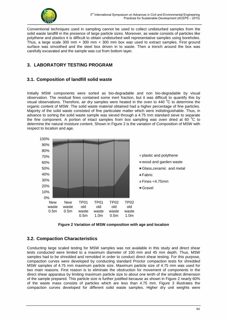
3rd International Symposium on Advances in Civil and Environmental Engineering Practices for Sustainable Development (ACEPS – 2015)
Conventional techniques used in sampling cannot be used to collect undisturbed samples from the solid waste landfill in the presence of large particle sizes. Moreover, as waste consists of particles like polythene and plastics it is difficult to obtain undisturbed well representative samples using boreholes. Thus, a large scale 300 mm × 300 mm × 300 mm box was used to extract samples. First ground surface was smoothed and the steel box driven in to waste. Then a trench around the box was carefully excavated and the sample was cut from bottom layer.
3. LABORATORY TESTING PROGRAM
3.1. Composition of landfill solid waste
Initially MSW components were sorted as bio-degradable and non bio-degradable by visual observation. The residual fines contained some inert fraction, but it was difficult to quantify this by visual observations. Therefore, air dry samples were heated in the oven to 440 0C to determine the organic content of MSW. The solid waste material obtained had a higher percentage of fine particles. Majority of the solid waste consisted of fine particulate matter which were indistinguishable. Thus, in advance to sorting the solid waste sample was sieved through a 4.75 mm standard sieve to separate the fine component. A portion of intact samples from box sampling was oven dried at 60 0C to determine the natural moisture content. Shown in Figure 2 is the variation of Composition of MSW with respect to location and age.
Figure 2 Variation of MSW composition with age and location
3.2. Compaction Characteristics
Conducting large scaled testing for MSW samples was not available in this study and direct shear tests conducted were limited to a maximum diameter of 100 mm and 45 mm depth. Thus, MSW samples had to be shredded and remolded in order to conduct direct shear testing. For this purpose, compaction curves were developed by conducting standard Proctor compaction tests for shredded MSW samples of 4.75 mm maximum particle size. Maximum particle size of 4.75 mm was used for two main reasons. First reason is to eliminate the obstruction for movement of components in the direct shear apparatus by limiting maximum particle size to about one tenth of the smallest dimension of the sample prepared. This particle size is further justified because as shown in Figure 2 nearly 60% of the waste mass consists of particles which are less than 4.75 mm. Figure 3 illustrates the compaction curves developed for different solid waste samples. Higher dry unit weights were
0%
10%
20%
30%
40%
50%
60%
70%
80%
90%
100%
Newwaste0.5m
Newwaste0.5m
TP01old
waste0.5m
TP01old
waste1.0m
TP02old
waste0.5m
TP02old
waste1.0m
plastic and polythene
wood and garden waste
Glass,ceramic and metal
Fabric
Fines <4.75mm
Gravel
94
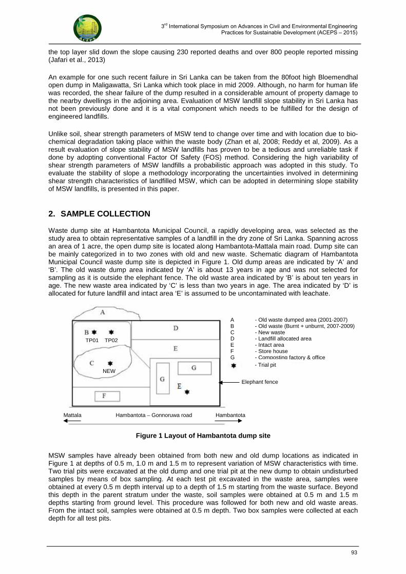
3rd International Symposium on Advances in Civil and Environmental Engineering Practices for Sustainable Development (ACEPS – 2015)
the top layer slid down the slope causing 230 reported deaths and over 800 people reported missing (Jafari et al., 2013)
An example for one such recent failure in Sri Lanka can be taken from the 80foot high Bloemendhal open dump in Maligawatta, Sri Lanka which took place in mid 2009. Although, no harm for human life was recorded, the shear failure of the dump resulted in a considerable amount of property damage to the nearby dwellings in the adjoining area. Evaluation of MSW landfill slope stability in Sri Lanka has not been previously done and it is a vital component which needs to be fulfilled for the design of engineered landfills.
Unlike soil, shear strength parameters of MSW tend to change over time and with location due to bio-chemical degradation taking place within the waste body (Zhan et al, 2008; Reddy et al, 2009). As a result evaluation of slope stability of MSW landfills has proven to be a tedious and unreliable task if done by adopting conventional Factor Of Safety (FOS) method. Considering the high variability of shear strength parameters of MSW landfills a probabilistic approach was adopted in this study. To evaluate the stability of slope a methodology incorporating the uncertainties involved in determining shear strength characteristics of landfilled MSW, which can be adopted in determining slope stability of MSW landfills, is presented in this paper.
2. SAMPLE COLLECTION
Waste dump site at Hambantota Municipal Council, a rapidly developing area, was selected as the study area to obtain representative samples of a landfill in the dry zone of Sri Lanka. Spanning across an area of 1 acre, the open dump site is located along Hambantota-Mattala main road. Dump site can be mainly categorized in to two zones with old and new waste. Schematic diagram of Hambantota Municipal Council waste dump site is depicted in Figure 1. Old dump areas are indicated by ‘A’ and ‘B’. The old waste dump area indicated by ‘A’ is about 13 years in age and was not selected for sampling as it is outside the elephant fence. The old waste area indicated by ‘B’ is about ten years in age. The new waste area indicated by ‘C’ is less than two years in age. The area indicated by ‘D’ is allocated for future landfill and intact area ‘E’ is assumed to be uncontaminated with leachate.
Figure 1 Layout of Hambantota dump site
MSW samples have already been obtained from both new and old dump locations as indicated in Figure 1 at depths of 0.5 m, 1.0 m and 1.5 m to represent variation of MSW characteristics with time. Two trial pits were excavated at the old dump and one trial pit at the new dump to obtain undisturbed samples by means of box sampling. At each test pit excavated in the waste area, samples were obtained at every 0.5 m depth interval up to a depth of 1.5 m starting from the waste surface. Beyond this depth in the parent stratum under the waste, soil samples were obtained at 0.5 m and 1.5 m depths starting from ground level. This procedure was followed for both new and old waste areas. From the intact soil, samples were obtained at 0.5 m depth. Two box samples were collected at each depth for all test pits.
Elephant fence
A - Old waste dumped area (2001-2007) B - Old waste (Burnt + unburnt, 2007-2009) C - New waste D - Landfill allocated area E - Intact area F - Store house G - Composting factory & office
- Trial pit
Mattala Hambantota – Gonnoruwa road Hambantota
TP01 TP02
NEW
93