Estimation of Mutual Information by the Fuzzy Histogram · The integrals of theEquation 3measure the smoothness of the probability density functions. When the pdf’s are smooth,

Noname manuscript No.(will be inserted by the editor)

Estimation of Mutual Information by the Fuzzy Histogram

Maryam Amir Haeri ·Mohammad Mehdi Ebadzadeh

the date of receipt and acceptance should be inserted later

Abstract Mutual Information (MI) is an important dependency measure betweenrandom variables, due to its tight connection with information theory. It hasnumerous applications, both in theory and practice. However, when employed inpractice, it is often necessary to estimate the MI from available data. There areseveral methods to approximate the MI, but arguably one of the simplest andmost widespread techniques is the histogram-based approach.

This paper suggests the use of fuzzy partitioning for the histogram-based MIestimation. It uses a general form of fuzzy membership functions, which includesthe class of crisp membership functions as a special case. It is accordingly shownthat the average absolute error of the fuzzy-histogram method is less than that ofthe naıve histogram method. Moreover, the accuracy of our technique is compara-ble, and in some cases superior to the accuracy of the Kernel Density Estimation(KDE) method, which is one of the best MI estimation methods. Furthermore,the computational cost of our technique is significantly less than that of the KDE.

The new estimation method is investigated from different aspects, such asaverage error, bias and variance. Moreover, we explore the usefulness of thefuzzy-histogram MI estimator in a real-world bioinformatics application. Ourexperiments show that, in contrast to the naıve histogram MI estimator, thefuzzy-histogram MI estimator is able to reveal all dependencies between the gene-expression data.

1 Introduction

Finding dependencies between random variables is an important task in manyproblems [1, 7, 14, 15], such as independent component analysis and feature se-lection. There are several measures that quantify the linear dependency betweenrandom variables, such as the Pearson correlation coefficient and the Spearman

Maryam Amir HaeriDepartment of Computer Engineering and Information Technology, Amirkabir University ofTechnology, Tehran, IranE-mail: [email protected]

Mohammad Mahdi EbadzadehDepartment of Computer Engineering and Information Technology, Amirkabir University ofTechnology, Tehran, IranE-mail: [email protected]

Estimation of Mutual Information by the Fuzzy Histogram 2

correlation coefficient. Such measures are not sufficient to quantify the general de-pendency between two random variables. On the other hand, Mutual Information

(MI) provides a general dependency measure between two random variables. MIcan measure any kind of relationship between the random variables.

The MI of two random variables depends on their distributions. However, mostof the time, it is required to find the mutual information of two variables whosedistributions are unknown, and only some samples from them are available. Toestimate the MI, one has to estimate the entropies or probability density functions(pdf’s) from the data samples.

There are several methods to estimate the mutual information from finite sam-ples. The most popular method for MI estimation is the histogram-based method[11], which partitions the space into several bins, and counts the number of ele-ments in each bin. This method is very easy and efficient from the computationalpoint of view. However, the approximation given by the counting process is dis-continuous, and the estimation is very sensitive to the number of bins [9, 13].

Moon et al. [12] presented another MI estimation approach called Kernel Den-

sity Estimation (KDE). KDE utilizes kernels to approximate pdf’s. Probabilitydensity functions can be estimated by the superposition of a set of kernel func-tions. In general, KDE provides a high quality estimation for MI. However, it isvery time-consuming and computationally intensive [8, 9, 14].

Kraskov et al. [8] suggested the K-Nearest Neighbors (KNN) method to esti-mate the mutual information. This method is based on estimating entropies fromKNN distances.

Another method of estimating the MI is adaptive partitioning, which wasintroduced by Darbellay and Vajda [4]. This method is based on the histogramapproach, but it is not parametric. In their approach, the partition is improveduntil the conditional independence has been achieved in the bins.

Wang et al. [16] suggested a nonlinear correlation measure called NonlinearCorrelation Coefficient (NCC). Their measure is based on the mutual informationcarried by the rank sequences of the original data. Unlike the mutual information,NCC takes values from the closed interval [0,1].

The accumulation process in the histogram-based method depends on theanswer of the question “whether a sample x belongs to the bin ai or not.” However,because of the vagueness in the boundaries of histogram bins, it is not possibleto answer this question exactly. A reasonable solution to overcome this problemis using fuzziness in the partitioning [2, 9].

Loquin and Strauss [9, 10] suggested a histogram density estimator based ona fuzzy partition. They proved the consistency of this estimator based on theMean Square Error (MSE) [10]. Moreover, they showed that the main advantageof this estimator is the enhancement of the robustness of the histogram densityestimator, with respect to arbitrary partitioning. Since the mutual information oftwo variables is a function of the density of the variables, using histogram esti-mator based on fuzzy partitioning (fuzzy-histogram) can improve the histogramMI estimator.

This paper introduces the fuzzy-histogram mutual-information estimator. Thefuzzy-histogram MI estimator uses the fuzzy partitioning. We consider a generalform of fuzzy membership functions whose shapes are controlled by a parameter.By increasing this parameter, the membership functions tend from fuzzy towardscrisp. Using these general membership functions, it is demonstrated that the his-


togram method with fuzzy partitioning outperforms the naıve histogram method(based on the average absolute error).

The rest of this paper is organized as follows: Section 2 is dedicated to thehistogram MI estimator. In Section 3 the fuzzy-histogram method for estimatingmutual information is introduced. Section 4 investigates different aspects of thefuzzy-histogram MI estimator. Section 5 compares the fuzzy-histogram MI esti-mator, histogram MI estimator, and KDE in a bioinformatics application. Finally,Section 6 concludes the paper.

2 Preliminaries

In this section, the histogram MI estimation method is explained briefly. Moreover,the bias and variance of this method are studied.

2.1 The Histogram MI Estimator

The mutual information of two continuous random variables X and Y is definedas I(X,Y ) =

∫∫X,Y

p(x, y) log p(x,y)p(x)p(y)dxdy. Here, p(x, y) is the joint pdf of X and

Y , and p(x) and p(y) are the marginal pdf’s of X and Y , respectively.Suppose that we have N simultaneous samples of X and Y . To estimate the MI

by the histogram method, the variable X is partitioned into MX bins, and variableY is partitioned into MY bins. We call the ith bin of X, ai (where 1 ≤ i ≤ MX),and the jth bin of Y , bj (where 1 ≤ j ≤ MY ). Furthermore, p(ai) is defined asthe probability of observing a sample of X in the bin ai. The probability p(ai) isestimated by the relative frequency of samples of X observed in the cell ai, andis equal to ki

N . Here, ki is the number of samples of X observed in the bin ai.Moreover, p(ai, bj) is defined as the probability of observing a sample of (X,Y) inthe bin (ai, bj) (i.e. x lies in the bin ai and y in the bin bj), and is approximated

bykijN . Here, kij is the number of samples observed in the bin (ai, bj).Hence, the mutual information of X and Y is estimated as follows:

I(X,Y ) =∑ij

kijN

logkijN

kikj. (1)

2.2 Bias of the Histogram MI Estimator

Based on [11], the histogram-based estimator is a biased estimator. The total biasis the sum of N-bias and R-bias. Here, these two types of bias are explained briefly.

– N-bias: This bias is caused by the finite sample size and depends on the samplesize N . When the mutual information I(X,Y ) is estimated from a finite samplesize N by the histogram estimator, the N-bias is as follows [11]:

∆I(X,Y )N-bias =MXMY −MX −MY + 1

2N, (2)

where MX and MY are the number of histogram bins. Note that the N-biasdoes not depend on the probability distribution of the variables, and only de-pends on the sample size and the number of bins. According to the Equation 2,when N tends to infinity, the N-bias tends to zero.

– R-Bias: Insufficient representation of the probability distribution function(pdf) by the histogram method leads to the R-bias. R-bias is specified bythe estimation method and the pdf’s of the variables, and it is caused by twoseparate sources: (1) the limited integration area, and (2) the finite resolution.Moddemeijer [11] showed that the bias caused by the limited integration areais negligible in comparison with the bias caused by the finite resolution, and it


can be ignored. For the histogram MI estimator, they demonstrated that theR-biased caused by the finite resolution is as follows:

∆I(X,Y )R-bias =

∫ +∞

−∞

1

24p(x)

(∂p(x)

∂x

)2

(∆x)2dx+

∫ +∞

−∞

1

24p(y)

(∂p(y)

∂y

)2

(∆y)2dy

−∫ +∞

−∞

∫ +∞

−∞

1

24p(x, y)

((∂p(x, y)

∂x

)2

(∆x)2 +

(∂p(x, y)

∂y

)2

(∆y)2)dxdy .

(3)

The integrals of the Equation 3 measure the smoothness of the probabilitydensity functions. When the pdf’s are smooth, the first derivatives are ap-proximately equal to zero. Hence, the squared derivatives are almost zero andR-bias is minimized.

The N-bias of the histogram MI estimator leads to overestimation, and theR-bias leads to underestimation. By increasing the number of bins (decreasingthe bin length) the R-bias is decreased, and the N-bias is increased. Hence, thenumber of bins makes a trade-off between the N-bias and the R-bias.

2.3 Variance of the Histogram MI Estimator

A good estimator must have a low variance. The variance of the histogram esti-mator of the mutual information can be written as follows [11]:

VAR[I(X,Y )] ≈ 1

NVAR

logp(x, y)

p(x−)p(y−)

, (4)

where x and y are the vectors of N simultaneous samples of X and Y .The variance of the histogram MI estimator approximately does not depend

on the cell sizes, except in the following cases: (1) the number of bins is one, (2)the number of bins tends to infinity. In these cases, the variance is equal to zero.

3 Fuzzy-Histogram Method for Estimating Mutual Information

In this section, we present the fuzzy-histogram MI estimator. As mentioned in theintroduction, Loquin and Strauss [10] showed that the fuzzy-histogram densityestimator can improve the robustness of the histogram density estimator. Sinceestimating the mutual information depends on the estimation of the probabilitiesp(x), p(y) and p(x, y), utilizing fuzzy partitioning can improve the histogram MIestimator. In this section, a general form for membership function is suggested.The shape of membership functions is controlled by a parameter called β. As βtends to infinity, the membership functions tend to crisp functions. By using thisgeneral form, it is possible to test whether fuzzification can improve the histogrammethod, and which membership functions are better in estimating the MI by thefuzzy histogram method.

3.1 Fuzzy Partitioning

Let D = [a, b] ⊂ R be the domain of variable X. We want to partition D asfollows. Let γ1 < γ2 < · · · < γn be n ≥ 3 points of D such that γ1 = a andγn = b. Let the length of the bins be equal to h. Therefore, γk = a + (k − 1)h.Now define two other points γ0 = a− h and γn+1 = b+ h. Consider the extendeddomain D′ = [γ0, γn+1] ⊂ R. Define n fuzzy subsets A1, A2, . . . , An on the extendeddomain D′, with membership functions µA1

(x), µA2(x), . . . , µAn(x). These fuzzy

sets should satisfy the following properties:


1. µAk(γk) = 1;2. µAk(x) monotonically increases on [γ0, γk], and µAk(x) monotonically decreases

on [γk, γn+1];3. ∀x ∈ D′, ∃k such that µAk(x) > 0.

Some examples of membership functions with mentioned properties are listedbelow:

– the crisp partition: KA(x) = 1[−12, 12](x),

– the cosine partition: 12

(cos(πx) + 1

)1[−1,1](x),

– the triangular partition: (1− |x|) 1[−1,1](x),– the generalized normal partition as described next.

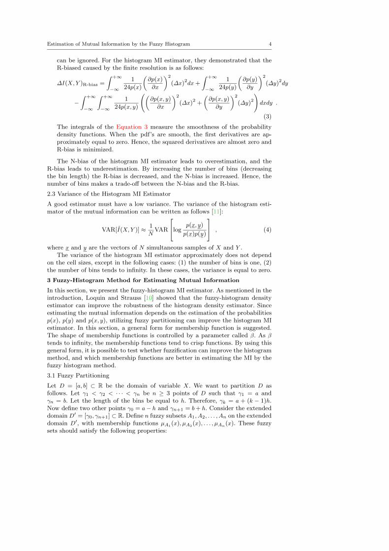
Fig. 1 illustrates a fuzzy partitioning of interval [-10,10] with triangular mem-bership functions.

−15 −10 −5 0 5 10 150

0.5

1

x

µ(x)

Fig. 1: Fuzzy partitioning with triangular membership functions. Here, the numberof bins is equal to 6.

A good choice for the membership functions is the Generalized Normal Func-tion (GNF), which provides a general from for the membership functions.

GNF is a parametric continuous function. GNF is the pdf of the generalized

normal distribution. This type of function adds a shape parameter to the normalfunction. The formula of the generalized normal function is as follows:

f(x) =β

2αΓ (1/β)e−(|x− µ|/α

)β, (5)

where Γ is the gamma function (Γ (z) =∫∞0e−ttz−1dt).

By changing the parameter β of this function, its shape is changed. Whenβ = 2, the shape of the function is like the pdf of the normal distribution. Fur-thermore, when β = 1 it is like the pdf of the Laplace distribution and its shapeis similar to the triangular function. By increasing the parameter β, the shape ofthe function gradually becomes similar to the pulse function. Moreover, α is thescale parameter.

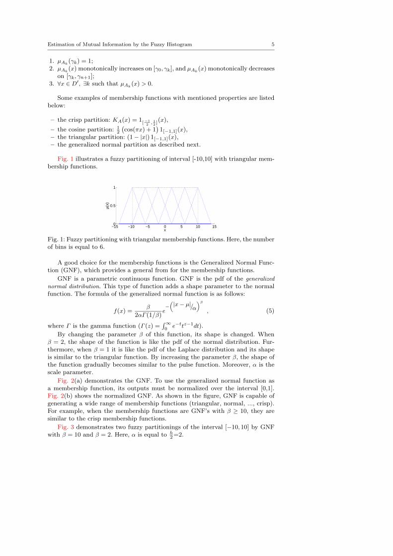
Fig. 2(a) demonstrates the GNF. To use the generalized normal function asa membership function, its outputs must be normalized over the interval [0,1].Fig. 2(b) shows the normalized GNF. As shown in the figure, GNF is capable ofgenerating a wide range of membership functions (triangular, normal, ..., crisp).For example, when the membership functions are GNF’s with β ≥ 10, they aresimilar to the crisp membership functions.

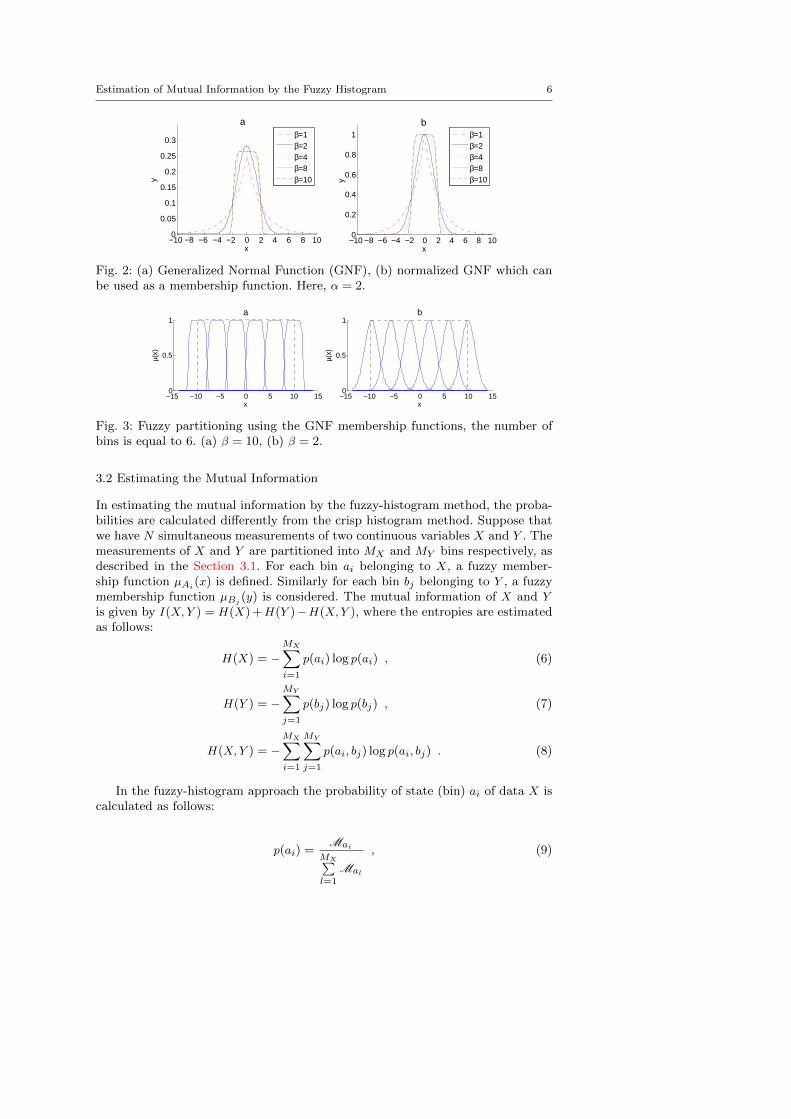
Fig. 3 demonstrates two fuzzy partitionings of the interval [−10, 10] by GNFwith β = 10 and β = 2. Here, α is equal to h

2=2.


−10 −8 −6 −4 −2 0 2 4 6 8 100

0.2

0.4

0.6

0.8

1

x

y

b

β=1β=2β=4β=8β=10

−10 −8 −6 −4 −2 0 2 4 6 8 100

0.05

0.1

0.15

0.2

0.25

0.3

x

y

a

β=1β=2β=4β=8β=10

Fig. 2: (a) Generalized Normal Function (GNF), (b) normalized GNF which canbe used as a membership function. Here, α = 2.

−15 −10 −5 0 5 10 150

0.5

1

x

µ(x)

a

−15 −10 −5 0 5 10 150

0.5

1

x

µ(x)

b

Fig. 3: Fuzzy partitioning using the GNF membership functions, the number ofbins is equal to 6. (a) β = 10, (b) β = 2.

3.2 Estimating the Mutual Information

In estimating the mutual information by the fuzzy-histogram method, the proba-bilities are calculated differently from the crisp histogram method. Suppose thatwe have N simultaneous measurements of two continuous variables X and Y . Themeasurements of X and Y are partitioned into MX and MY bins respectively, asdescribed in the Section 3.1. For each bin ai belonging to X, a fuzzy member-ship function µAi(x) is defined. Similarly for each bin bj belonging to Y , a fuzzymembership function µBj (y) is considered. The mutual information of X and Y

is given by I(X,Y ) = H(X) +H(Y )−H(X,Y ), where the entropies are estimatedas follows:

H(X) = −MX∑i=1

p(ai) log p(ai) , (6)

H(Y ) = −MY∑j=1

p(bj) log p(bj) , (7)

H(X,Y ) = −MX∑i=1

MY∑j=1

p(ai, bj) log p(ai, bj) . (8)

In the fuzzy-histogram approach the probability of state (bin) ai of data X iscalculated as follows:

p(ai) =Mai

MX∑l=1

Mal

, (9)


where Mai is the sum of membership values of samples of X belonging to thefuzzy set Ai:

Mai =N∑k=1

µAi(xk) . (10)

In the crisp histogram MI estimation method, the probability of observing asample of X in the bin ai is estimated by the relative frequency of samples ofX observed in the bin ai, and it equals to ki

N . In the fuzzy histogram method,this probability is estimated by the fraction in Equation 9: the nominator is thesum of membership values of samples of X belonging to the fuzzy set Ai, and thedenominator is the sum of membership values of samples of X belonging to allfuzzy sets. Hence, the crisp histogram is a special case of the fuzzy histogram,where the membership value of each sample belonging to a bin is either one orzero. Thus, in this case,

∑Nk=1 µAi(xk) is equal to the frequency of samples of X

observed in the cell ai, and∑MX

l=1 Mal is equal to the N . Therefore, Equation 9 isequivalent to the relative frequency of the crisp case.

Similarly, the probability of state (bin) bj of data Y and Mbj are as follows:

p(bj) =Mbj

MY∑s=1

Mbs

, (11)

Mbj =N∑k=1

µBj (yk) . (12)

In the crisp histogram method, p(ai, bj) is defined as the probability of observ-ing a sample (x, y) of (X,Y ) in the bin (ai, bj) (where x lies in the bin ai and y inthe bin bj). Let kij be the number of samples which lie in the bin (ai, bj). Based

on the frequentist approach to probability, p(ai, bj) ≈kijN .

Now denote by (Ai, Bj) the fuzzy set associated with the bin (ai, bj). Letµ(Ai,Bj) be the membership function of (Ai, Bj). We use the product for definingthe membership function, that is, for any data-point (xk, yk), we have µ(Ai,Bj)(xk, yk) =µAi(xk) · µBj (yk).

Following the analogy of the crisp case, the frequentist approach suggeststhat the probability p(ai, bj) can be estimated by the relative sum of membershipvalues of samples of (X,Y ) belonging to the fuzzy set (Ai, Bj). Therefore, the jointprobability of the bin (ai, bj) is computed by:

p(ai, bj) =Maibj

MX∑l=1

MY∑s=1

Malbs

, (13)

where Maibj is obtained by the following equation:

Maibj =N∑k=1

µ(Ai,Bj)(xk, yk) =N∑k=1

µAi(xk) · µBj (yk) . (14)

Using the sum-product instead of max-min or max-product is natural dueto the analogy between the fuzzy and crisp cases, and the way one counts thedata-points lying in each bin. In other words, the summation of membershipvalues in the fuzzy method plays a similar role as counting the number of samples


observed in the bin (ai, bj) in the crisp case. Additionally, similar to p(ai), thecrisp histogram is a special case of the fuzzy histogram; because in the crispcase, if a sample belongs to a bin (ai, bj), its membership value is 1, and it is 0otherwise. Thus, in the crisp case, p(ai, bj) as computed by Equation 13 is equalto the relative frequency of samples belonging to the bin (ai, bj).

4 Experimental Results

In this section, the fuzzy-histogram mutual information estimator is investigatedfrom different aspects. Firstly, in a simple experiment, the fuzzy-histogram MIestimator is compared with the histogram estimator over independent variables.In the second part, the effects of the parameters of the fuzzy-histogram estima-tor, including the shape of the membership functions, and the number of bins areinvestigated for three different distributions. In the third part, the accuracy andthe running time of the fuzzy-histogram estimator are compared with those of thehistogram estimator, and the KDE. The fourth experiment compares the bias ofthe fuzzy-histogram estimator with the histogram estimator. The fifth experimentinvestigates the variance of the fuzzy-histogram estimator. The sixth experimentcompares different dependency measures on the data with different degrees of de-pendency. The final experiment is devoted to comparing the histogram estimator,fuzzy-histogram estimator, and the KDE in a real-world application.

4.1 Mutual Information of Independent Variables

0 200 400 600 800 10000

0.2

0.4

0.6

0.8

1

N

Est

imat

ed M

I

(a) Number of Bins=5

0 200 400 600 800 10000

0.2

0.4

0.6

0.8

1

N

Est

imat

ed M

I

(b) Number of Bins=10

0 200 400 600 800 10000

0.2

0.4

0.6

0.8

1

N

Est

imat

ed M

I

(c) Number of Bins=15

Fuzzy Histogram Estimator Histogram Estimator

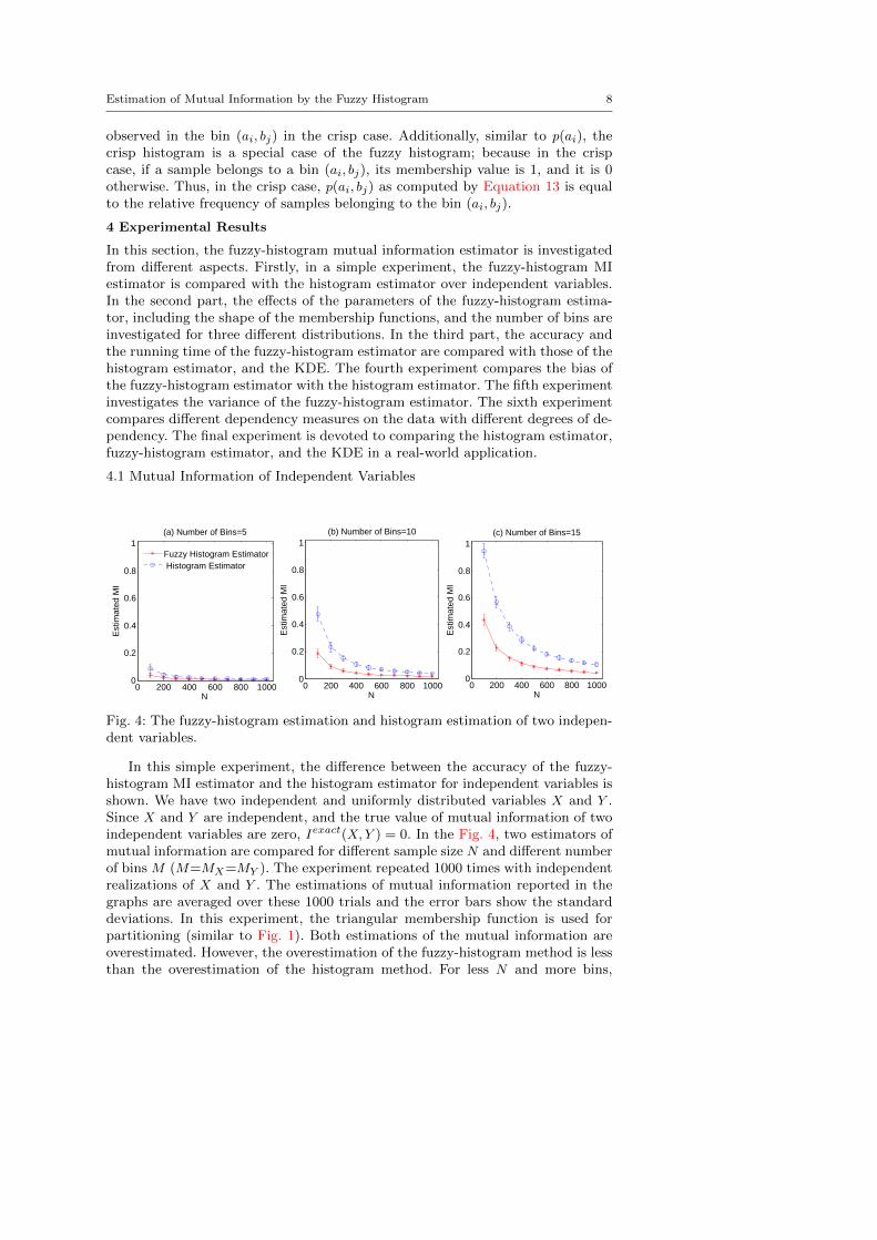
Fig. 4: The fuzzy-histogram estimation and histogram estimation of two indepen-dent variables.

In this simple experiment, the difference between the accuracy of the fuzzy-histogram MI estimator and the histogram estimator for independent variables isshown. We have two independent and uniformly distributed variables X and Y .Since X and Y are independent, and the true value of mutual information of twoindependent variables are zero, Iexact(X,Y ) = 0. In the Fig. 4, two estimators ofmutual information are compared for different sample size N and different numberof bins M (M=MX=MY ). The experiment repeated 1000 times with independentrealizations of X and Y . The estimations of mutual information reported in thegraphs are averaged over these 1000 trials and the error bars show the standarddeviations. In this experiment, the triangular membership function is used forpartitioning (similar to Fig. 1). Both estimations of the mutual information areoverestimated. However, the overestimation of the fuzzy-histogram method is lessthan the overestimation of the histogram method. For less N and more bins,


the difference between the two methods are more considerable. Thus, the fuzzy-histogram estimator provides more accurate estimation for independent variables,especially when the number of samples is few.

Additionally, the experimental overestimation of the histogram estimator isconsistent with the theoretical N-bias. For example, when N = 100 and the num-ber of bins is equal to 10, the theoretical overestimation is as follows:

E[I − Iexcat] =(10− 1)(10− 1)

2 ∗ 100≈ 0.41 ,

and the experimental N-bias for the histogram estimator is equal to 0.47. However,N-bias of the fuzzy-histogram estimator is less. In this case (N = 100), it is equalto 0.18. In the Section 4.4 more investigations are conducted on the bias of thefuzzy-histogram estimator.

4.2 The Effects of the Parameters of the Fuzzy-Histogram Method

In this experiment, the effects of the parameters of the fuzzy-histogram MI esti-mator are investigated by experimental analysis for three distributions. To find anappropriate membership function, the generalized normal function (GNF) (Equa-tion 5) is used. As mentioned in Section 3, generalized normal function is a para-metric continuous function (see Fig. 2). By changing the parameter β of thisfunction its shape is changed. When β = 2, the shape of the function is like thepdf of the normal distribution. Furthermore, when β = 1, it is like the pdf ofthe Laplace distribution and its shape is similar to the triangular function. Byincreasing the parameter β, the shape of the function gradually becomes similarto the pulse function. Moreover, α is the scale parameter.

Hence, the fuzzy-histogram estimator with generalized normal membershipfunction, has three important parameters, β, and α, which indicate the shape andscale of membership function and the number of bins.

Here, the impacts of parameters of the fuzzy-histogram MI estimator are in-vestigated for data with three distributions, bivariate normal, bivariate gamma-exponential, and bivariate ordered Weinman exponential distribution. In the fol-lowing, these distributions and their exact mutual information between their vari-ates are brought.

1. Bivariate Normal Distribution: the pdf of this distribution is as follows:

p(x, y) =1

2πσ1σ2√

1− ρ2e−z

2(1−ρ2) , (15)

where z = (x−µ1)2

σ21− 2ρ(x−µ1)(y−µ2)

σ1σ2+ (y−µ2)

2

σ22

and ρ = corr(X,Y ).

The exact mutual information between the variates X and Y of the bivariatenormal distribution with the correlation coefficient ρ is [11]:

I(X,Y ) =1

2log

(1

1− ρ2

). (16)

2. Bivariate Gamma Exponential Distribution: the pdf of this distribution is[3, 17]:

p(x, y) =θθ21 θ3

Γ (θ2)xθ2e−θ1x−θ3xy . (17)

The exact mutual information between the variates of this distribution is [3]:

I(X,Y ) = ψ(θ2)− ln(θ2) +1

θ2, (18)


where ψ(z) is the digamma function ψ(z) = dd(z) lnΓ (z) = Γ ′(z)

Γ (z) .

−4 −2 0 2 4−4−2

024

x

y

ρ=0

−4 −2 0 2 4−4−2

024

x

y

ρ=0.1

−4 −2 0 2 4−4−2

024

x

y

ρ=0.2

−4 −2 0 2 4−4−2

024

x

y

ρ=0.3

−4 −2 0 2 4−4−2

024

x

y

ρ=0.4

−4 −2 0 2 4−4−2

024

x

y

ρ=0.5

−4 −2 0 2 4−4−2

024

x

y

ρ=0.6

−4 −2 0 2 4−4−2

024

x

yρ=0.7

−4 −2 0 2 4−4−2

024

x

y

ρ=0.8

−4 −2 0 2 4−4−2

024

x

y

ρ=0.9

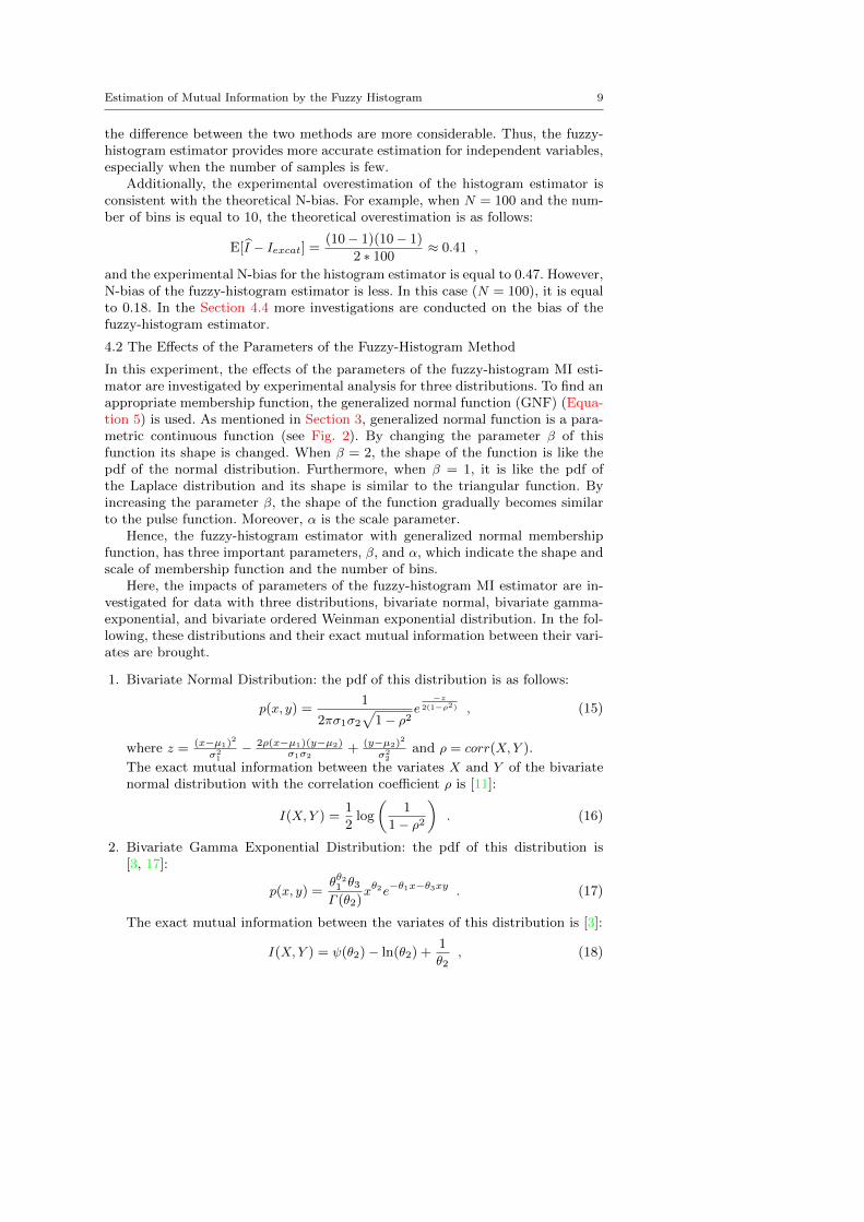
Fig. 5: Data with bivariate normal distribution with different correlation coeffi-cients ρ.

0 10 20 300

2

x

y

θ2=1

0 10 20 300

2

x

y

θ2=3

0 10 20 300

2

x

y

θ2=5

0 10 20 300

2

x

y

θ2=7

0 10 20 300

2

x

y

θ2=9

0 10 20 300

2

x

y

θ2=11

0 10 20 300

2

x

y

θ2=13

0 10 20 300

2

x

y

θ2=15

0 10 20 300

2

x

y

θ2=17

0 10 20 300

2

x

y

θ2=19

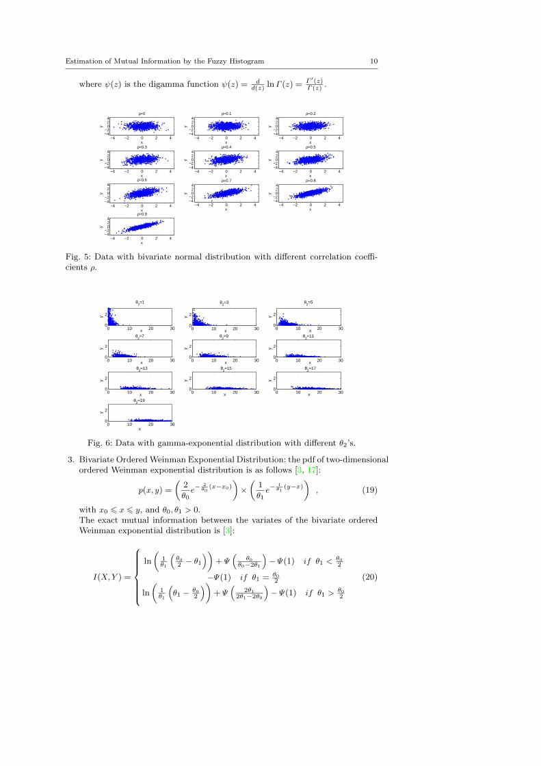
Fig. 6: Data with gamma-exponential distribution with different θ2’s.

3. Bivariate Ordered Weinman Exponential Distribution: the pdf of two-dimensionalordered Weinman exponential distribution is as follows [3, 17]:

p(x, y) =

(2

θ0e− 2θ0

(x−x0)

)×(

1

θ1e− 1θ1

(y−x))

, (19)

with x0 6 x 6 y, and θ0, θ1 > 0.The exact mutual information between the variates of the bivariate orderedWeinman exponential distribution is [3]:

I(X,Y ) =

ln

(1θ1

(θ02 − θ1

))+ Ψ

(θ0

θ0−2θ1

)− Ψ(1) if θ1 <

θ02

−Ψ(1) if θ1 = θ02

ln

(1θ1

(θ1 − θ0

2

))+ Ψ

(2θ1

2θ1−2θ0

)− Ψ(1) if θ1 >

θ02

(20)


In each of these distributions, the exact MI depends on some parameters of thedistribution. For bivariate normal distribution, the mutual information between itsvariates depends only on the correlation coefficient ρ. For the gamma-exponentialdistribution, MI depends on the parameter θ2, and for the ordered Weinmanexponential distribution, it depends on θ0 and θ1 or precisely on the proportionθ1/θ0.

Here, we want to find appropriate parameters of the fuzzy-histogram MI es-timator for each distribution, such that for different data driven from that dis-tribution with different exact MI, the average absolute error is minimized. Forexample, for the normal distribution, we want to find appropriate parameter val-ues among several parameter values such that for different bivariate normal datawith different ρ the average absolute error is minimized.

Thus, for this experiment, different realizations were generated from each dis-tribution with different parameter settings. Bivariate normal samples were gen-erated with 10 different correlation coefficient ρ = {0, 0.1, .., 0.8, 0.9}. The mean

vector and the covariance matrix are set to Mean =

[00

]and

∑=

[1 ρρ 1

]respec-

tively.Various realizations of the bivariate normal distribution with different ρ are

shown in the Fig. 5, to illustrate graphically the relation between the variates ofthis distribution. Here, the sample size N is 500.

For the bivariate gamma-exponential distribution samples were generated withθ1, θ3 = 1 and θ2 = {1, 2, . . . , 19, 20}. Fig. 6 illustrates several realizations of thisdistribution with different parameter values.

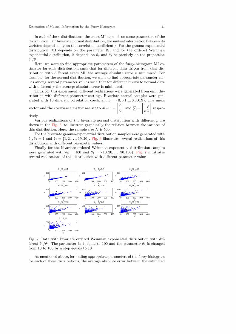
Finally for the bivariate ordered Weinman exponential distribution sampleswere generated with θ0 = 100 and θ1 = {10, 20, . . . , 90, 100}. Fig. 7 illustratesseveral realizations of this distribution with different parameter values.

0 100 200 300 4000

500

x

y

θ 1 / θ

0=0.1

0 100 200 300 4000

500

x

y

θ 1 / θ

0=0.2

0 100 200 300 4000

500

x

y

θ 1 / θ

0=0.3

0 100 200 300 4000

500

x

y

θ 1 / θ

0=0.4

0 100 200 300 4000

500

x

y

θ 1 / θ

0=0.5

0 100 200 300 4000

500

x

y

θ 1 / θ

0=0.6

0 100 200 300 4000

500

x

y

θ 1 / θ

0=0.7

0 100 200 300 4000

500

x

y

θ 1 / θ

0=0.8

0 100 200 300 4000

500

x

y

θ 1 / θ

0=0.9

0 100 200 300 4000

500

x

y

θ 1 / θ

0=1

Fig. 7: Data with bivariate ordered Weinman exponential distribution with dif-ferent θ1/θ0. The parameter θ0 is equal to 100 and the parameter θ1 is changedfrom 10 to 100 by a step equals to 10.

As mentioned above, for finding appropriate parameters of the fuzzy histogramfor each of these distributions, the average absolute error between the estimated


MI and exact MI is used. This average is computed over different realizations withdifferent parameter settings. Formally:

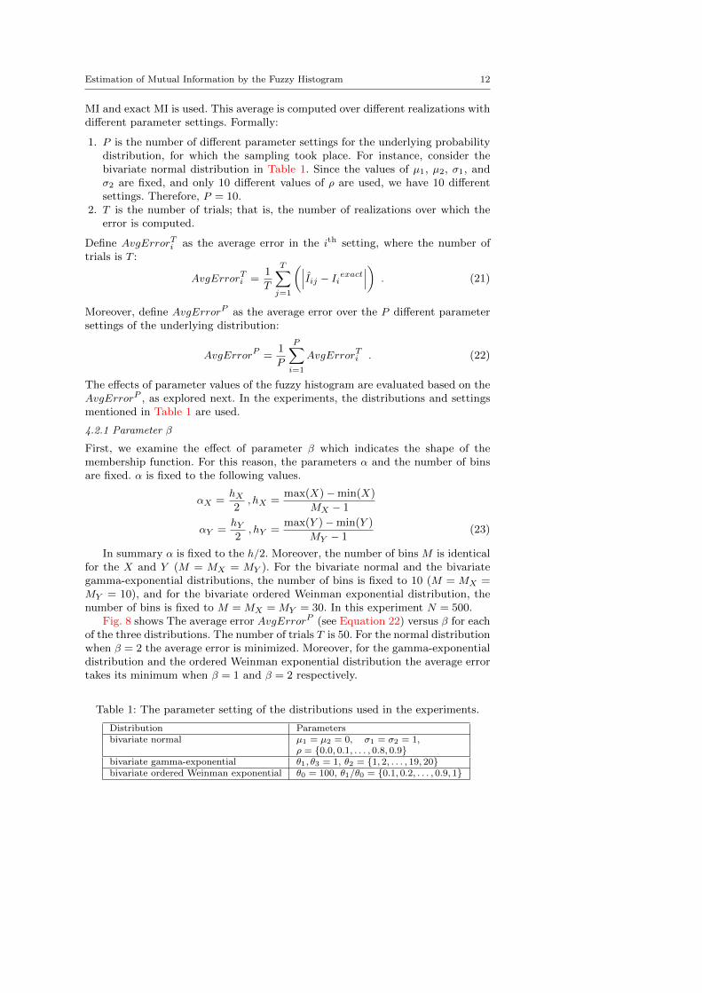
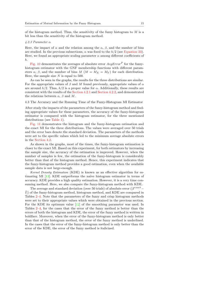
1. P is the number of different parameter settings for the underlying probabilitydistribution, for which the sampling took place. For instance, consider thebivariate normal distribution in Table 1. Since the values of µ1, µ2, σ1, andσ2 are fixed, and only 10 different values of ρ are used, we have 10 differentsettings. Therefore, P = 10.

2. T is the number of trials; that is, the number of realizations over which theerror is computed.

Define AvgErrorTi as the average error in the ith setting, where the number oftrials is T :

AvgErrorTi =1

T

T∑j=1

(∣∣∣Iij − Iiexact∣∣∣) . (21)

Moreover, define AvgErrorP as the average error over the P different parametersettings of the underlying distribution:

AvgErrorP =1

P

P∑i=1

AvgErrorTi . (22)

The effects of parameter values of the fuzzy histogram are evaluated based on theAvgErrorP , as explored next. In the experiments, the distributions and settingsmentioned in Table 1 are used.

4.2.1 Parameter β

First, we examine the effect of parameter β which indicates the shape of themembership function. For this reason, the parameters α and the number of binsare fixed. α is fixed to the following values.

αX =hX2, hX =

max(X)−min(X)

MX − 1

αY =hY2, hY =

max(Y )−min(Y )

MY − 1(23)

In summary α is fixed to the h/2. Moreover, the number of bins M is identicalfor the X and Y (M = MX = MY ). For the bivariate normal and the bivariategamma-exponential distributions, the number of bins is fixed to 10 (M = MX =MY = 10), and for the bivariate ordered Weinman exponential distribution, thenumber of bins is fixed to M = MX = MY = 30. In this experiment N = 500.

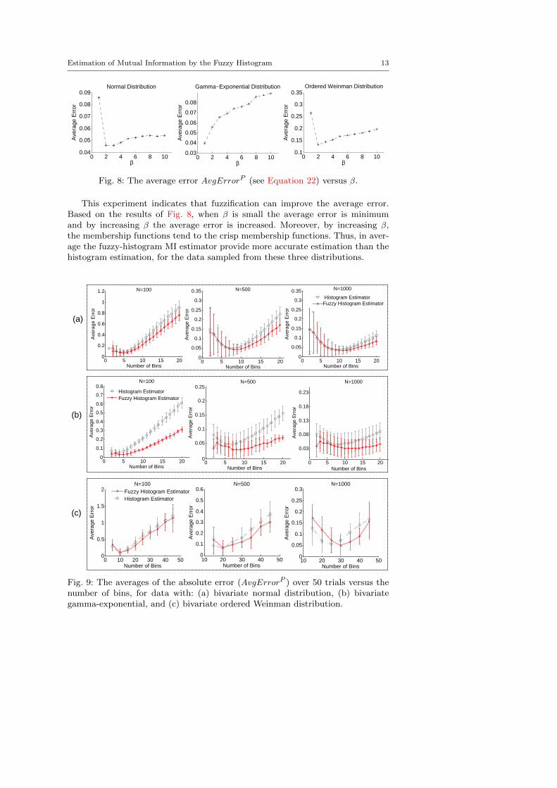
Fig. 8 shows The average error AvgErrorP (see Equation 22) versus β for eachof the three distributions. The number of trials T is 50. For the normal distributionwhen β = 2 the average error is minimized. Moreover, for the gamma-exponentialdistribution and the ordered Weinman exponential distribution the average errortakes its minimum when β = 1 and β = 2 respectively.

Table 1: The parameter setting of the distributions used in the experiments.

Distribution Parametersbivariate normal µ1 = µ2 = 0, σ1 = σ2 = 1,

ρ = {0.0, 0.1, . . . , 0.8, 0.9}bivariate gamma-exponential θ1, θ3 = 1, θ2 = {1, 2, . . . , 19, 20}bivariate ordered Weinman exponential θ0 = 100, θ1/θ0 = {0.1, 0.2, . . . , 0.9, 1}


0 2 4 6 8 100.04

0.05

0.06

0.07

0.08

0.09

β

Ave

rage

Err

or

Normal Distribution

0 2 4 6 8 100.03

0.04

0.05

0.06

0.07

0.08

β

Ave

rage

Err

or

Gamma−Exponential Distribution

0 2 4 6 8 100.1

0.15

0.2

0.25

0.3

0.35

β

Ave

rage

Err

or

Ordered Weinman Distribution

Fig. 8: The average error AvgErrorP (see Equation 22) versus β.

This experiment indicates that fuzzification can improve the average error.Based on the results of Fig. 8, when β is small the average error is minimumand by increasing β the average error is increased. Moreover, by increasing β,the membership functions tend to the crisp membership functions. Thus, in aver-age the fuzzy-histogram MI estimator provide more accurate estimation than thehistogram estimation, for the data sampled from these three distributions.

0 5 10 15 200

0.2

0.4

0.6

0.8

1

1.2

Number of Bins

Ave

rage

Err

or

N=100

0 5 10 15 200

0.05

0.1

0.15

0.2

0.25

0.3

0.35

Number of Bins

Ave

rage

Err

orN=1000

0 5 10 15 200

0.05

0.1

0.15

0.2

0.25

0.3

0.35

Number of Bins

Ave

rage

Err

or

N=500

Histogram EstimatorFuzzy Histogram Estimator

0 5 10 15 200

0.1

0.2

0.3

0.4

0.5

0.6

0.7

0.8

Number of Bins

Ave

rage

Err

or

N=100

0 5 10 15 200

0.05

0.1

0.15

0.2

0.25

Number of Bins

Ave

rage

Err

or

N=500

0 5 10 15 20

0.03

0.08

0.13

0.18

0.23

Number of Bins

Ave

rage

Err

or

N=1000


0 10 20 30 40 500

0.5

1

1.5

2

Number of Bins

Ave

rage

Err

or

N=100

10 20 30 40 500

0.1

0.2

0.3

0.4

0.5

0.6

Number of Bins

Ave

rage

Err

or

N=500

10 20 30 40 500

0.05

0.1

0.15

0.2

0.25

0.3

Number of Bins

Ave

rage

Err

or

N=1000Fuzzy Histogram EstimatorHistogram Estimator

(a)

(b)

(c)

Fig. 9: The averages of the absolute error (AvgErrorP ) over 50 trials versus thenumber of bins, for data with: (a) bivariate normal distribution, (b) bivariategamma-exponential, and (c) bivariate ordered Weinman distribution.

Estimation of Mutual Information by the Fuzzy Histogram 140.3h

0.4h

0.5h

0.6h

0.7h

0.8h

0.9h

510

1520

00.10.20.30.4

Number of Bins

β=1

α

Ave

rrag

e E

rror

0.3h0.4h

0.5h0.6h

0.7h0.8h

0.9h

510

1520

0

0.2

0.4

Number of Bins

β=2

α

Ave

rage

Err

or

0.3h0.4h

0.5h0.6h

0.7h0.8h

0.9h

510

1520

0

0.2

0.4

Number of Bins

β=3

α

Ave

rage

Err

or

0.3h

0.4h

0.5h

0.6h

0.7h

0.8h

0.9h

510

1520

00.10.20.30.4

Number of Bins

β=1

α

Ave

rrag

e E

rror

0.3h0.4h

0.5h0.6h

0.7h0.8h

0.9h

510

1520

0

0.2

0.4

Number of Bins

β=2

α

Ave

rage

Err

or0.3h

0.4h0.5h

0.6h0.7h

0.8h0.9h

510

1520

0

0.2

0.4

Number of Bins

β=3

α

Ave

rage

Err

or0.3h

0.4h0.5h

0.6h0.7h

0.8h0.9h

36

912

15

0

0.1

0.2

Number of Bins

β=3

α

Ave

rage

Err

or0.3h

0.4h0.5h

0.6h0.7h

0.8h0.9h

36

912

15

0

0.1

0.2

Number of Bins

β=1

α

Ave

rage

Err

or

0.3h0.4h

0.5h0.6h

0.7h0.8h

0.9h

36

912

15

0

0.1

0.2

Number of Bins

β=2

α

Ave

rage

Err

or

0.3h0.4h

0.5h0.6h

0.7h0.8h

0.9h

1520

2530

35

0

0.5

1

Number of Bins

β=1

α

Ave

rage

Err

or

0.3h0.4h

0.5h0.6h

0.7h0.8h

0.9h

1520

2530

35

0

0.5

1

Number of Bins

β=2

α

Ave

rage

Err

or

0.3h0.4h

0.5h0.6h

0.7h0.8h

0.9h

1520

2530

35

0

0.5

1

Number of Bins

β=3

α

Ave

rage

Err

or

(a)

(b)

(c)

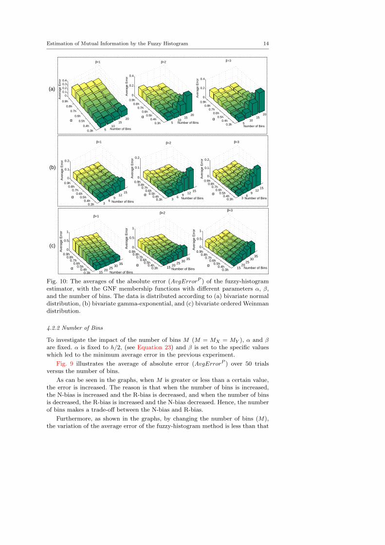
Fig. 10: The averages of the absolute error (AvgErrorP ) of the fuzzy-histogramestimator, with the GNF membership functions with different parameters α, β,and the number of bins. The data is distributed according to (a) bivariate normaldistribution, (b) bivariate gamma-exponential, and (c) bivariate ordered Weinmandistribution.

4.2.2 Number of Bins

To investigate the impact of the number of bins M (M = MX = MY ), α and β

are fixed. α is fixed to h/2, (see Equation 23) and β is set to the specific valueswhich led to the minimum average error in the previous experiment.

Fig. 9 illustrates the average of absolute error (AvgErrorP ) over 50 trialsversus the number of bins.

As can be seen in the graphs, when M is greater or less than a certain value,the error is increased. The reason is that when the number of bins is increased,the N-bias is increased and the R-bias is decreased, and when the number of binsis decreased, the R-bias is increased and the N-bias decreased. Hence, the numberof bins makes a trade-off between the N-bias and R-bias.

Furthermore, as shown in the graphs, by changing the number of bins (M),the variation of the average error of the fuzzy-histogram method is less than that


of the histogram method. Thus, the sensitivity of the fuzzy histogram to M is abit less than the sensitivity of the histogram method.

4.2.3 Parameter α

Here, the impact of α and the relation among the α, β, and the number of binsare studied. In the previous subsections, α was fixed to the h/2 (see Equation 23).Here, we found an appropriate scaling parameter α among different coefficients ofh.

Fig. 10 demonstrates the averages of absolute error AvgErrorP for the fuzzy-histogram estimator with the GNF membership functions with different param-eters α, β, and the number of bins M (M = MX = MY ) for each distribution.Here, the sample size N is equal to 500.

As can be seen in the graphs, the results for the three distributions are similar.For the appropriate values of β and M found previously, appropriate values of αare around h/2. Thus, h/2 is a proper value for α. Additionally, these results areconsistent with the results of the Section 4.2.1 and Section 4.2.2, and demonstratedthe relations between α, β and M .

4.3 The Accuracy and the Running Time of the Fuzzy-Histogram MI Estimator

After study the impacts of the parameters of the fuzzy-histogram method and find-ing appropriate values for these parameters, the accuracy of the fuzzy-histogramestimator is compared with the histogram estimator, for the three mentioneddistributions (see Table 1).

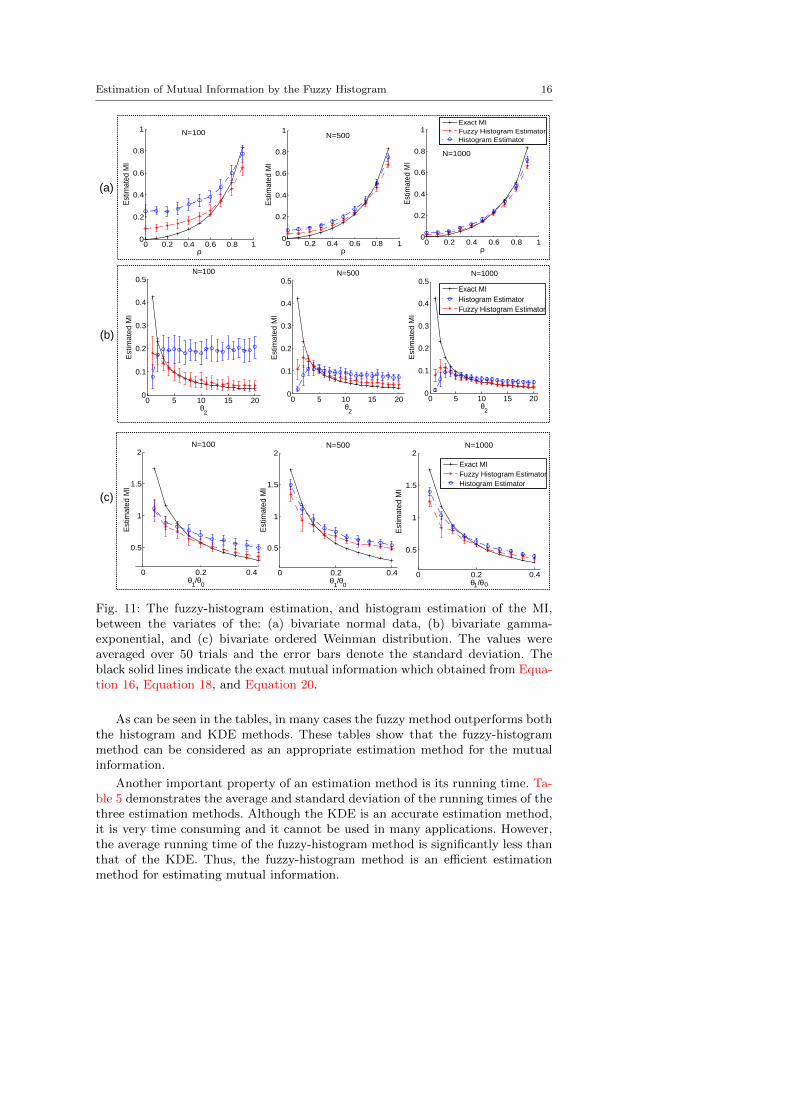
Fig. 11 demonstrates the histogram and the fuzzy-histogram estimation andthe exact MI for the three distributions. The values were averaged over 50 trialsand the error bars denote the standard deviation. The parameters of the methodswere set to the specific values which led to the minimum average absolute errorsin the Section 4.2.

As shown in the graphs, most of the times, the fuzzy-histogram estimation iscloser to the exact MI. Based on this experiment, for both estimators by increasingthe sample size, the accuracy of the estimation is improved. However, when thenumber of samples is few, the estimation of the fuzzy-histogram is considerablybetter than that of the histogram method. Hence, this experiment indicates thatthe fuzzy-histogram method provides a good estimation, even when the availablesample data is not large-enough.

Kernel Density Estimation (KDE) is known as an effective algorithm for es-timating MI [13]. KDE outperforms the naıve histogram estimator in terms ofaccuracy. KDE provides a high quality estimation. However, it is a very time con-suming method. Here, we also compare the fuzzy-histogram method with KDE.

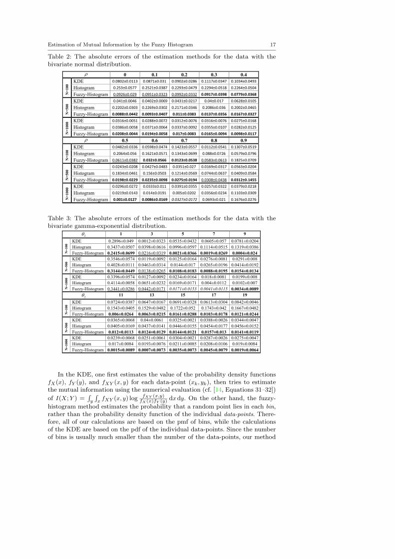
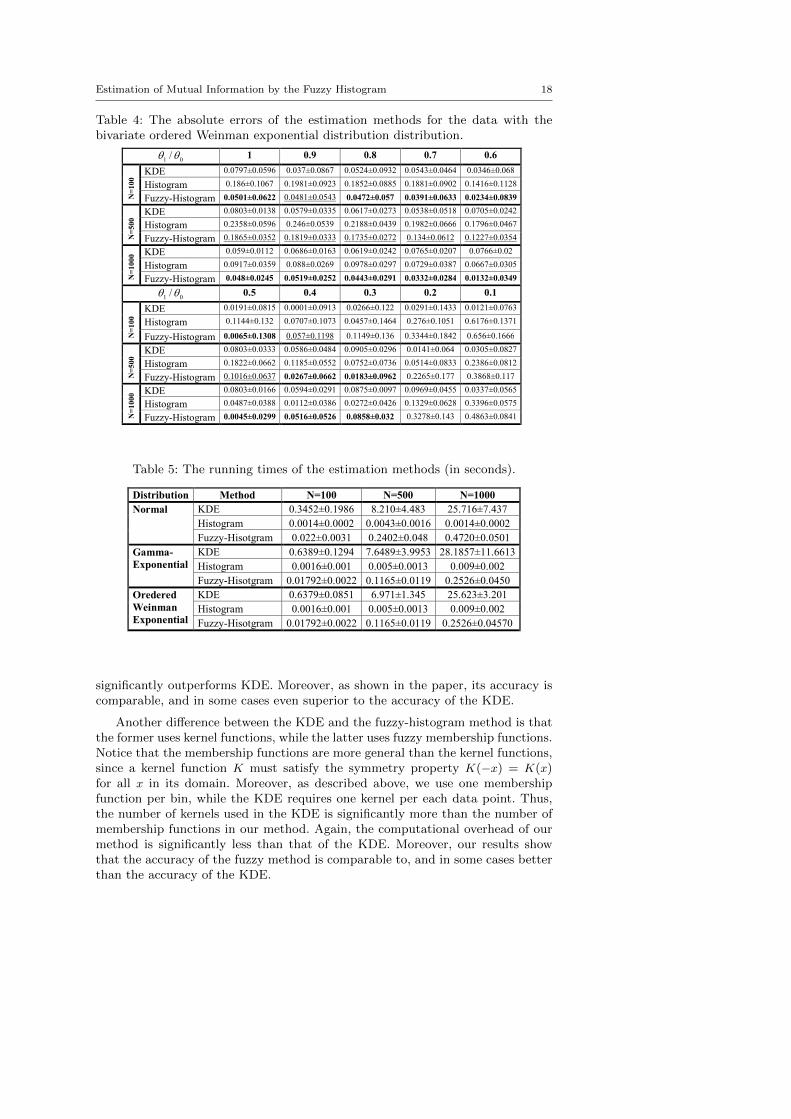
The average and standard deviation (over 50 trials) of absolute error (|Iexact−I|) of the fuzzy-histogram method, histogram method, and KDE are compared inTables 2–4. Note that the parameters of the fuzzy and crisp histogram methodswere set to their appropriate values which were obtained in the previous section.For the KDE its optimum value [12] of the smoothing parameter was used. InTables 2–4, for the cases that the error of the fuzzy method is better than theerrors of both the histogram and KDE, the error of the fuzzy method is written inboldface. Moreover, when the error of the fuzzy-histogram method is only betterthan that of the histogram method, the error of the fuzzy method is underlined.In the cases that the error of the fuzzy-histogram method is only better than theerror of the KDE, the error of the fuzzy method is italicized.


0 0.2 0.4

0.5

1

1.5

2

θ1/θ

0

Est

imat

ed M

I

N=100

0 0.2 0.4

0.5

1

1.5

2

θ1/θ

0

Est

imat

ed M

I

N=500

0 0.2 0.4

0.5

1

1.5

2

θ1/θ0

Est

imat

ed M

I

N=1000

Exact MIFuzzy Histogram EstimatorHistogram Estimator

Fuzzy Histogram EstimatorHistogram Estimator

(a)

(b)

(c)

0 0.2 0.4 0.6 0.8 10

0.2

0.4

0.6

0.8

1

ρ

Est

imat

ed M

I

N=1000

0 0.2 0.4 0.6 0.8 10

0.2

0.4

0.6

0.8

1

ρ

Est

imat

ed M

I

N=500

0 0.2 0.4 0.6 0.8 10

0.2

0.4

0.6

0.8

1

ρ

Est

imat

ed M

IN=100



0 5 10 15 200

0.1

0.2

0.3

0.4

0.5

θ2

Est

imat

ed M

IN=500

0 5 10 15 200

0.1

0.2

0.3

0.4

0.5

θ2

Est

imat

ed M

I

N=1000

0 5 10 15 200

0.1

0.2

0.3

0.4

0.5

θ2

Est

imat

ed M

I

N=100

Exact MIHistogram EstimatorFuzzy Histogram Estimator

Fig. 11: The fuzzy-histogram estimation, and histogram estimation of the MI,between the variates of the: (a) bivariate normal data, (b) bivariate gamma-exponential, and (c) bivariate ordered Weinman distribution. The values wereaveraged over 50 trials and the error bars denote the standard deviation. Theblack solid lines indicate the exact mutual information which obtained from Equa-tion 16, Equation 18, and Equation 20.

As can be seen in the tables, in many cases the fuzzy method outperforms boththe histogram and KDE methods. These tables show that the fuzzy-histogrammethod can be considered as an appropriate estimation method for the mutualinformation.

Another important property of an estimation method is its running time. Ta-ble 5 demonstrates the average and standard deviation of the running times of thethree estimation methods. Although the KDE is an accurate estimation method,it is very time consuming and it cannot be used in many applications. However,the average running time of the fuzzy-histogram method is significantly less thanthat of the KDE. Thus, the fuzzy-histogram method is an efficient estimationmethod for estimating mutual information.


Table 2: The absolute errors of the estimation methods for the data with thebivariate normal distribution.

0 0.1 0.2 0.3 0.4

N=

100

KDE 0.0802±0.0113 0.0871±0.031 0.0902±0.0286 0.1117±0.0347 0.1034±0.0493

Histogram 0.253±0.0577 0.2521±0.0387 0.2293±0.0479 0.2294±0.0518 0.2264±0.0504

Fuzzy-Histogram 0.0926±0.029 0.0951±0.0323 0.0992±0.0332 0.0917±0.0398 0.0779±0.0368

N=

500

KDE 0.041±0.0046 0.0402±0.0069 0.0431±0.0217 0.04±0.017 0.0628±0.0105

Histogram 0.2202±0.0303 0.2269±0.0302 0.2171±0.0346 0.2086±0.036 0.2002±0.0465

Fuzzy-Histogram 0.0088±0.0442 0.0093±0.0407 0.011±0.0383 0.0137±0.0356 0.0167±0.0327

N=

100

0 KDE 0.0316±0.0051 0.0288±0.0072 0.0312±0.0076 0.0316±0.0076 0.0275±0.0168

Histogram 0.0386±0.0058 0.0371±0.0064 0.0337±0.0092 0.0355±0.0107 0.0282±0.0125

Fuzzy-Histogram 0.0208±0.0044 0.0194±0.0058 0.017±0.0083 0.0165±0.0094 0.0098±0.0117

0.5 0.6 0.7 0.8 0.9

N=

100

KDE 0.0482±0.0336 0.0598±0.0474 0.1423±0.0557 0.0112±0.0541 0.1307±0.0519

Histogram 0.2064±0.056 0.1621±0.0571 0.1343±0.0699 0.088±0.0726 0.0579±0.0796

Fuzzy-Histogram 0.0611±0.0382 0.032±0.0566 0.0123±0.0538 0.0583±0.0613 0.1825±0.0709

N=

500

KDE 0.0243±0.0208 0.0427±0.0483 0.0351±0.027 0.0169±0.0317 0.0563±0.0204

Histogram 0.1834±0.0461 0.156±0.0503 0.1214±0.0569 0.0744±0.0637 0.0409±0.0584

Fuzzy-Histogram 0.0198±0.0229 0.0235±0.0098 0.0275±0.0194 0.0308±0.0438 0.0312±0.1455

N=

100

0 KDE 0.0296±0.0272 0.0333±0.011 0.0391±0.0355 0.0257±0.0322 0.0379±0.0218

Histogram 0.0219±0.0143 0.014±0.0191 0.005±0.0202 0.0356±0.0234 0.1103±0.0309

Fuzzy-Histogram 0.001±0.0127 0.0086±0.0169 0.0327±0.0172 0.0693±0.021 0.1676±0.0276

Table 3: The absolute errors of the estimation methods for the data with thebivariate gamma-exponential distribution.

2 1 3 5 7 9

N=

100

KDE 0.2896±0.049 0.0012±0.0323 0.0535±0.0432 0.0605±0.057 0.0781±0.0204

Histogram 0.3437±0.0507 0.0398±0.0616 0.0996±0.0597 0.1114±0.0515 0.1319±0.0386

Fuzzy-Histogram 0.2415±0.0699 0.0216±0.0319 0.0021±0.0366 0.0019±0.0269 0.0004±0.024

N=

500

KDE 0.3546±0.0574 0.0119±0.0092 0.0125±0.0164 0.0276±0.0081 0.0291±0.008

Histogram 0.4028±0.0111 0.0463±0.0314 0.0144±0.017 0.0265±0.0196 0.0414±0.0192

Fuzzy-Histogram 0.3144±0.0449 0.0138±0.0265 0.0108±0.0183 0.0088±0.0195 0.0154±0.0134

N=

1000

KDE 0.3396±0.0574 0.0127±0.0092 0.0234±0.0164 0.018±0.0081 0.0199±0.008

Histogram 0.4114±0.0058 0.0651±0.0232 0.0169±0.0171 0.004±0.0112 0.0102±0.007

Fuzzy-Histogram 0.3441±0.0286 0.0442±0.0171 0.0171±0.0153 0.0041±0.0115 0.0034±0.0089

2 11 13 15 17 19

N=

100

KDE 0.0724±0.0387 0.0647±0.0167 0.0691±0.0328 0.0613±0.0304 0.0842±0.0046

Histogram 0.1543±0.0405 0.1529±0.0482 0.1722±0.052 0.1743±0.042 0.1667±0.0482

Fuzzy-Histogram 0.006±0.0264 0.0063±0.0215 0.0161±0.0288 0.0103±0.0178 0.0121±0.0244

N=

500

KDE 0.0365±0.0068 0.04±0.0061 0.0325±0.0021 0.0388±0.0026 0.0344±0.0047

Histogram 0.0405±0.0169 0.0437±0.0141 0.0446±0.0155 0.0454±0.0177 0.0456±0.0152

Fuzzy-Histogram 0.012±0.0113 0.0124±0.0129 0.0144±0.0121 0.0157±0.013 0.0141±0.0119

N=

1000

KDE 0.0239±0.0068 0.0251±0.0061 0.0304±0.0021 0.0287±0.0026 0.0275±0.0047

Histogram 0.017±0.0084 0.0193±0.0076 0.0211±0.0085 0.0208±0.0106 0.019±0.0084

Fuzzy-Histogram 0.0015±0.0089 0.0007±0.0073 0.0035±0.0073 0.0045±0.0079 0.0019±0.0064

In the KDE, one first estimates the value of the probability density functionsfX(x), fY (y), and fXY (x, y) for each data-point (xk, yk), then tries to estimatethe mutual information using the numerical evaluation (cf. [14, Equations 31–32])

of I(X;Y ) =∫y

∫xfXY (x, y) log fXY (x,y)

fX(x)fY (y) dxdy. On the other hand, the fuzzy-

histogram method estimates the probability that a random point lies in each bin,rather than the probability density function of the individual data-points. There-fore, all of our calculations are based on the pmf of bins, while the calculationsof the KDE are based on the pdf of the individual data-points. Since the numberof bins is usually much smaller than the number of the data-points, our method


Table 4: The absolute errors of the estimation methods for the data with thebivariate ordered Weinman exponential distribution distribution.

1 0/ 1 0.9 0.8 0.7 0.6

N=

100

KDE 0.0797±0.0596 0.037±0.0867 0.0524±0.0932 0.0543±0.0464 0.0346±0.068

Histogram 0.186±0.1067 0.1981±0.0923 0.1852±0.0885 0.1881±0.0902 0.1416±0.1128

Fuzzy-Histogram 0.0501±0.0622 0.0481±0.0543 0.0472±0.057 0.0391±0.0633 0.0234±0.0839

N=

500

KDE 0.0803±0.0138 0.0579±0.0335 0.0617±0.0273 0.0538±0.0518 0.0705±0.0242

Histogram 0.2358±0.0596 0.246±0.0539 0.2188±0.0439 0.1982±0.0666 0.1796±0.0467

Fuzzy-Histogram 0.1865±0.0352 0.1819±0.0333 0.1735±0.0272 0.134±0.0612 0.1227±0.0354

N=

1000

KDE 0.059±0.0112 0.0686±0.0163 0.0619±0.0242 0.0765±0.0207 0.0766±0.02

Histogram 0.0917±0.0359 0.088±0.0269 0.0978±0.0297 0.0729±0.0387 0.0667±0.0305

Fuzzy-Histogram 0.048±0.0245 0.0519±0.0252 0.0443±0.0291 0.0332±0.0284 0.0132±0.0349

1 0/ 0.5 0.4 0.3 0.2 0.1

N=

100

KDE 0.0191±0.0815 0.0001±0.0913 0.0266±0.122 0.0291±0.1433 0.0121±0.0763

Histogram 0.1144±0.132 0.0707±0.1073 0.0457±0.1464 0.276±0.1051 0.6176±0.1371

Fuzzy-Histogram 0.0065±0.1308 0.057±0.1198 0.1149±0.136 0.3344±0.1842 0.656±0.1666

N=

500

KDE 0.0803±0.0333 0.0586±0.0484 0.0905±0.0296 0.0141±0.064 0.0305±0.0827

Histogram 0.1822±0.0662 0.1185±0.0552 0.0752±0.0736 0.0514±0.0833 0.2386±0.0812

Fuzzy-Histogram 0.1016±0.0637 0.0267±0.0662 0.0183±0.0962 0.2265±0.177 0.3868±0.117

N=

1000 KDE 0.0803±0.0166 0.0594±0.0291 0.0875±0.0097 0.0969±0.0455 0.0337±0.0565

Histogram 0.0487±0.0388 0.0112±0.0386 0.0272±0.0426 0.1329±0.0628 0.3396±0.0575

Fuzzy-Histogram 0.0045±0.0299 0.0516±0.0526 0.0858±0.032 0.3278±0.143 0.4863±0.0841

Table 5: The running times of the estimation methods (in seconds).

Distribution Method N=100 N=500 N=1000

Normal KDE 0.3452±0.1986 8.210±4.483 25.716±7.437

Histogram 0.0014±0.0002 0.0043±0.0016 0.0014±0.0002

Fuzzy-Hisotgram 0.022±0.0031 0.2402±0.048 0.4720±0.0501

Gamma-Exponential

KDE 0.6389±0.1294 7.6489±3.9953 28.1857±11.6613

Histogram 0.0016±0.001 0.005±0.0013 0.009±0.002

Fuzzy-Hisotgram 0.01792±0.0022 0.1165±0.0119 0.2526±0.0450

Oredered Weinman Exponential

KDE 0.6379±0.0851 6.971±1.345 25.623±3.201

Histogram 0.0016±0.001 0.005±0.0013 0.009±0.002

Fuzzy-Hisotgram 0.01792±0.0022 0.1165±0.0119 0.2526±0.04570

significantly outperforms KDE. Moreover, as shown in the paper, its accuracy iscomparable, and in some cases even superior to the accuracy of the KDE.

Another difference between the KDE and the fuzzy-histogram method is thatthe former uses kernel functions, while the latter uses fuzzy membership functions.Notice that the membership functions are more general than the kernel functions,since a kernel function K must satisfy the symmetry property K(−x) = K(x)for all x in its domain. Moreover, as described above, we use one membershipfunction per bin, while the KDE requires one kernel per each data point. Thus,the number of kernels used in the KDE is significantly more than the number ofmembership functions in our method. Again, the computational overhead of ourmethod is significantly less than that of the KDE. Moreover, our results showthat the accuracy of the fuzzy method is comparable to, and in some cases betterthan the accuracy of the KDE.


4.4 Bias of the Fuzzy-Histogram Estimator

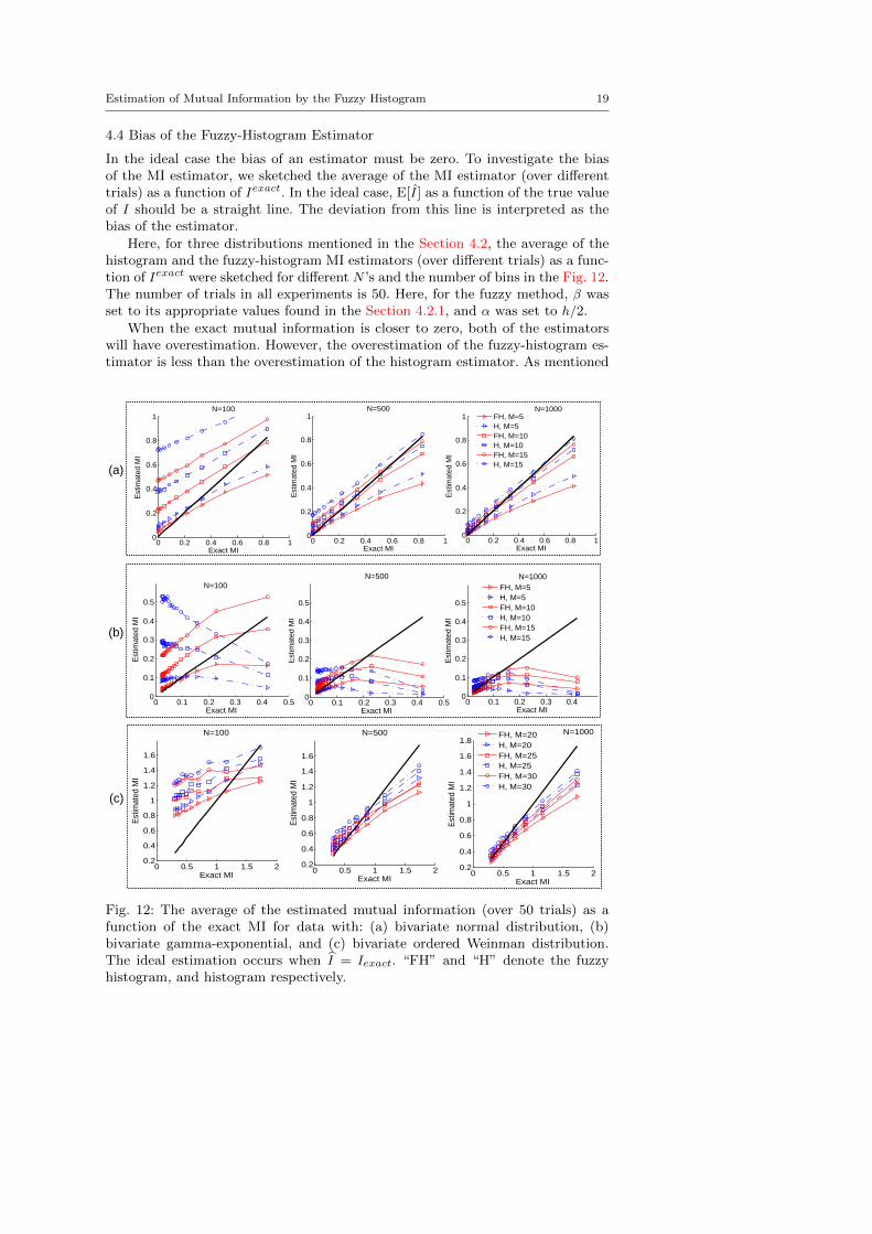
In the ideal case the bias of an estimator must be zero. To investigate the biasof the MI estimator, we sketched the average of the MI estimator (over differenttrials) as a function of Iexact. In the ideal case, E[I] as a function of the true valueof I should be a straight line. The deviation from this line is interpreted as thebias of the estimator.

Here, for three distributions mentioned in the Section 4.2, the average of thehistogram and the fuzzy-histogram MI estimators (over different trials) as a func-tion of Iexact were sketched for different N ’s and the number of bins in the Fig. 12.The number of trials in all experiments is 50. Here, for the fuzzy method, β wasset to its appropriate values found in the Section 4.2.1, and α was set to h/2.

When the exact mutual information is closer to zero, both of the estimatorswill have overestimation. However, the overestimation of the fuzzy-histogram es-timator is less than the overestimation of the histogram estimator. As mentioned

0 0.2 0.4 0.6 0.8 10

0.2

0.4

0.6

0.8

1

Exact MI

Est

imat

ed M

I

N=500

0 0.2 0.4 0.6 0.8 10

0.2

0.4

0.6

0.8

1

Exact MI

Est

imat

ed M

I

N=1000

0 0.2 0.4 0.6 0.8 10

0.2

0.4

0.6

0.8

1

Exact MI

Est

imat

ed M

I

N=100

FH, M=5H, M=5FH, M=10H, M=10FH, M=15H, M=15

0 0.1 0.2 0.3 0.4 0.50

0.1

0.2

0.3

0.4

0.5

Exact MI

Est

imat

ed M

I

N=500

0 0.1 0.2 0.3 0.40

0.1

0.2

0.3

0.4

0.5

Exact MI

Est

imat

ed M

I

N=1000

0 0.1 0.2 0.3 0.4 0.50

0.1

0.2

0.3

0.4

0.5

Exact MI

Est

imat

ed M

I

N=100


(a)

(b)

(c)

0 0.5 1 1.5 20.2

0.4

0.6

0.8

1

1.2

1.4

1.6

Exact MI

Est

imat

ed M

I

N=100

0 0.5 1 1.5 20.2

0.4

0.6

0.8

1

1.2

1.4

1.6

Exact MI

Est

imat

ed M

I

N=500

0 0.5 1 1.5 20.2

0.4

0.6

0.8

1

1.2

1.4

1.6

1.8

Exact MI

Est

imat

ed M

I

N=1000


Fig. 12: The average of the estimated mutual information (over 50 trials) as afunction of the exact MI for data with: (a) bivariate normal distribution, (b)bivariate gamma-exponential, and (c) bivariate ordered Weinman distribution.The ideal estimation occurs when I = Iexact. “FH” and “H” denote the fuzzyhistogram, and histogram respectively.


in Section 2.2 this overestimation is called N-bias and caused by the finite sam-ple size. Hence, the N-bias of the fuzzy-histogram estimator is less. Moreover,increasing the sample size and decreasing the number of bins can decrease theoverestimation in both estimators.

When the exact mutual information becomes greater, the underestimationor R-bias appears. In both estimators, increasing the number of bins decreasesthe underestimation. Here, there is a trade-off for the number of bins, becauseby increasing the number of bins the underestimation (R-bias) reveals, howeverincreasing the number of bins leads to increasing the N-bias.

For the gamma-exponential distribution the R-bias of the fuzzy-histogramestimator is less than the R-bias of the histogram estimator. However, for thenormal and ordered Weinman exponential distributions the R-bias (underestima-tion) of the fuzzy-histogram estimator is greater than the R-bias of the histogramestimator.

4.5 Variance of the Fuzzy-Histogram Estimator

In this part, the variances of the fuzzy-histogram and the histogram MI estimatorsare compared. The number of trials in all experiments is 50. Here, for the fuzzymethod, β was set to its appropriate values found in the Section 4.2.1, and α wasset to h/2.

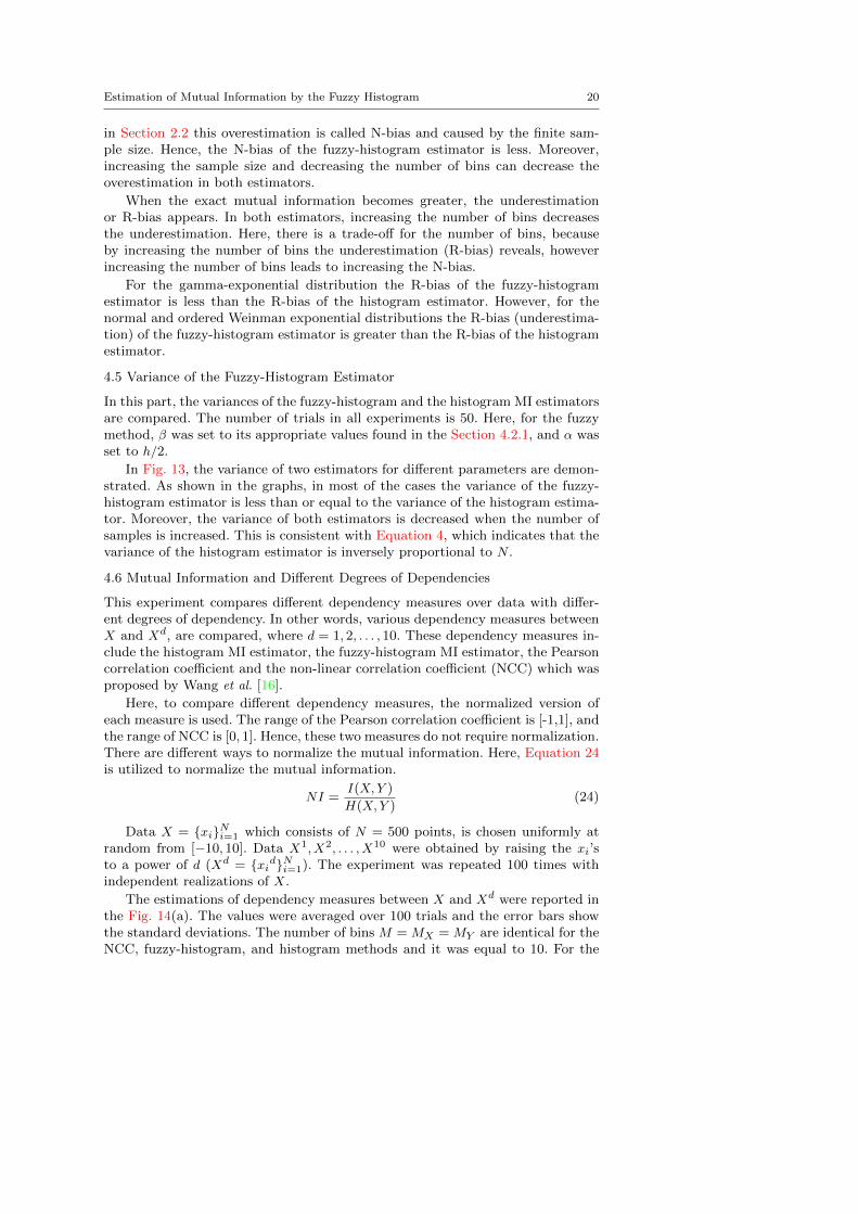
In Fig. 13, the variance of two estimators for different parameters are demon-strated. As shown in the graphs, in most of the cases the variance of the fuzzy-histogram estimator is less than or equal to the variance of the histogram estima-tor. Moreover, the variance of both estimators is decreased when the number ofsamples is increased. This is consistent with Equation 4, which indicates that thevariance of the histogram estimator is inversely proportional to N .

4.6 Mutual Information and Different Degrees of Dependencies

This experiment compares different dependency measures over data with differ-ent degrees of dependency. In other words, various dependency measures betweenX and Xd, are compared, where d = 1, 2, . . . , 10. These dependency measures in-clude the histogram MI estimator, the fuzzy-histogram MI estimator, the Pearsoncorrelation coefficient and the non-linear correlation coefficient (NCC) which wasproposed by Wang et al. [16].

Here, to compare different dependency measures, the normalized version ofeach measure is used. The range of the Pearson correlation coefficient is [-1,1], andthe range of NCC is [0, 1]. Hence, these two measures do not require normalization.There are different ways to normalize the mutual information. Here, Equation 24is utilized to normalize the mutual information.

NI =I(X,Y )

H(X,Y )(24)

Data X = {xi}Ni=1 which consists of N = 500 points, is chosen uniformly atrandom from [−10, 10]. Data X1, X2, . . . , X10 were obtained by raising the xi’sto a power of d (Xd = {xid}Ni=1). The experiment was repeated 100 times withindependent realizations of X.

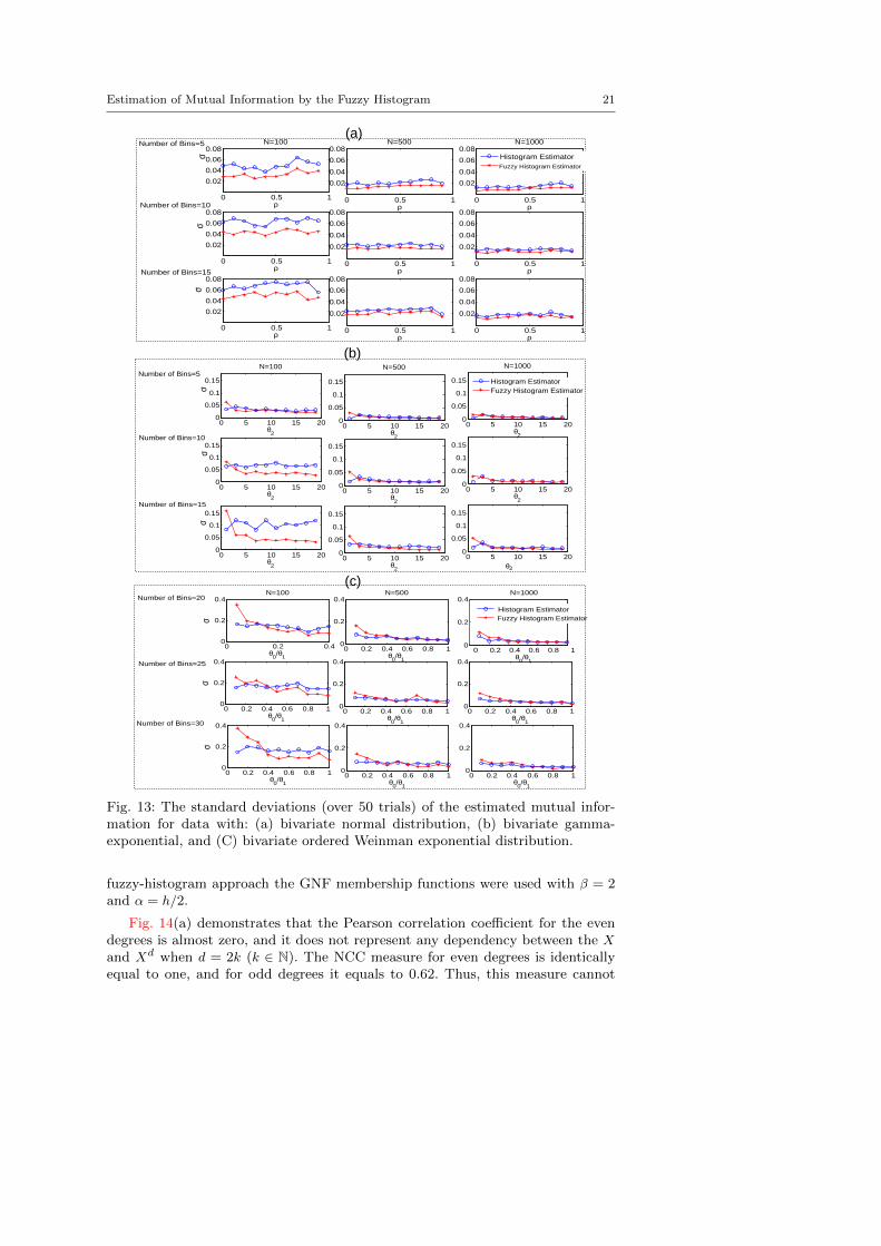
The estimations of dependency measures between X and Xd were reported inthe Fig. 14(a). The values were averaged over 100 trials and the error bars showthe standard deviations. The number of bins M = MX = MY are identical for theNCC, fuzzy-histogram, and histogram methods and it was equal to 10. For the


0 0.2 0.4 0.6 0.8 10

0.2

0.4

θ0/θ

1

N=500

0 0.2 0.4 0.6 0.8 10

0.2

0.4

θ0/θ

1

σ

0 0.2 0.4 0.6 0.8 10

0.2

0.4

θ0/θ

1

0 0.2 0.4 0.6 0.8 10

0.2

0.4

θ0/θ

1

0 0.2 0.4 0.6 0.8 10

0.2

0.4

θ0/θ

1

σ

0 0.2 0.4 0.6 0.8 10

0.2

0.4

θ0/θ

1

0 0.2 0.4 0.6 0.8 10

0.2

0.4

θ0/θ

1

0 0.2 0.40

0.2

0.4

θ0/θ

1

σ

N=100

0 0.2 0.4 0.6 0.8 10

0.2

0.4

θ0/θ

1

N=1000


Number of Bins=25

Number of Bins=20

Number of Bins=30

(a)

(b)

(c)

0 5 10 15 200

0.05

0.1

0.15

θ2

N=500

0 5 10 15 200

0.05

0.1

0.15

θ2

N=1000

0 5 10 15 200

0.05

0.1

0.15

θ2

σ

0 5 10 15 200

0.05

0.1

0.15

θ2

0 5 10 15 200

0.05

0.1

0.15

θ2

0 5 10 15 200

0.05

0.1

0.15

θ2

σ

0 5 10 15 200

0.05

0.1

0.15

θ2

0 5 10 15 200

0.05

0.1

0.15

θ2

0 5 10 15 200

0.05

0.1

0.15

θ2

σ

N=100


Number of Bins=5

Number of Bins=10

0 0.5 1

0.02

0.04

0.06

0.08

ρ

σ

N=100

0 0.5 1

0.02

0.04

0.06

0.08

ρ

N=500

0 0.5 1

0.02

0.04

0.06

0.08

ρ

N=1000

0 0.5 1

0.02

0.04

0.06

0.08

ρ

σ

0 0.5 1

0.02

0.04

0.06

0.08

ρ0 0.5 1

0.02

0.04

0.06

0.08

ρ

0 0.5 1

0.02

0.04

0.06

0.08

ρ

σ

0 0.5 1

0.02

0.04

0.06

0.08

ρ0 0.5 1

0.02

0.04

0.06

0.08

ρ

Histogram EstimatorFuzzy Histogram EstimatorBin Numbers=5

Bin Numbers=10

Bin Numbers=15

0 0.5 1

0.02

0.04

0.06

0.08

ρσ

N=100

0 0.5 1

0.02

0.04

0.06

0.08

ρ

N=500

0 0.5 1

0.02

0.04

0.06

0.08

ρ

N=1000

0 0.5 1

0.02

0.04

0.06

0.08

ρ

σ

0 0.5 1

0.02

0.04

0.06

0.08

ρ0 0.5 1

0.02

0.04

0.06

0.08

ρ

0 0.5 1

0.02

0.04

0.06

0.08

ρ

σ

0 0.5 1

0.02

0.04

0.06

0.08

ρ0 0.5 1

0.02

0.04

0.06

0.08

ρ


Number of Bins=5

Number of Bins=10

Number of Bins=15

Number of Bins=15

Fig. 13: The standard deviations (over 50 trials) of the estimated mutual infor-mation for data with: (a) bivariate normal distribution, (b) bivariate gamma-exponential, and (C) bivariate ordered Weinman exponential distribution.

fuzzy-histogram approach the GNF membership functions were used with β = 2and α = h/2.

Fig. 14(a) demonstrates that the Pearson correlation coefficient for the evendegrees is almost zero, and it does not represent any dependency between the Xand Xd when d = 2k (k ∈ N). The NCC measure for even degrees is identicallyequal to one, and for odd degrees it equals to 0.62. Thus, this measure cannot


1 2 3 4 5 6 7 8 9 100

0.2

0.4

0.6

0.8

1

d

Dep

ende

ncy

Mea

sure

Normalized Histogram MI Estimator Normalized Fuzzy Histogram MI Estimator Pearson CorrelationNCC

1 2 3 4 5 6 7 8 9 10

0

0.5

1

d

Dep

ende

ncy

Mea

sure

(a) (b)

Fig. 14: The dependency measures for the data with different degrees of depen-dency. (a) Dependency between X and Xd, (b) dependency between |X| and |Xd|.

distinguish between the different degrees of dependency. However, the normal-ized mutual information (both the fuzzy-histogram estimation and the histogramestimation) can indicate the dependencies between X and Xd for different d’s.

For further investigation, the experiment was repeated for the |X| and |Xd|,and the results were demonstrated in the Fig. 14(b). Here, Pearson correlationand NCC of the even degrees are not zero. However, NCC cannot distinguishbetween different degrees of dependency, because it uses rank orders of variablesinstead of the original data. Moreover, in this case, the behavior of the correlationcoefficient and the normalized mutual information are similar to each other.

This experiment demonstrated the advantage of MI as a measure of depen-dency between variables. MI can indicate dependency in some cases that NCCand the correlation coefficient cannot.

5 Application in Gene Expression

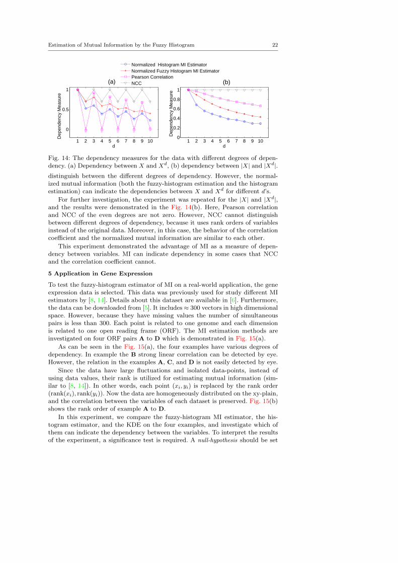
To test the fuzzy-histogram estimator of MI on a real-world application, the geneexpression data is selected. This data was previously used for study different MIestimators by [8, 14]. Details about this dataset are available in [6]. Furthermore,the data can be downloaded from [5]. It includes ≈ 300 vectors in high dimensionalspace. However, because they have missing values the number of simultaneouspairs is less than 300. Each point is related to one genome and each dimensionis related to one open reading frame (ORF). The MI estimation methods areinvestigated on four ORF pairs A to D which is demonstrated in Fig. 15(a).

As can be seen in the Fig. 15(a), the four examples have various degrees ofdependency. In example the B strong linear correlation can be detected by eye.However, the relation in the examples A, C, and D is not easily detected by eye.

Since the data have large fluctuations and isolated data-points, instead ofusing data values, their rank is utilized for estimating mutual information (sim-ilar to [8, 14]). In other words, each point (xi, yi) is replaced by the rank order(rank(xi), rank(yi)). Now the data are homogeneously distributed on the xy-plain,and the correlation between the variables of each dataset is preserved. Fig. 15(b)shows the rank order of example A to D.

In this experiment, we compare the fuzzy-histogram MI estimator, the his-togram estimator, and the KDE on the four examples, and investigate which ofthem can indicate the dependency between the variables. To interpret the resultsof the experiment, a significance test is required. A null-hypothesis should be set


−0.2 0 0.2 0.4−0.4

−0.25

−0.1

0.05

0.2

YKL148C

YLR

264W

D

−0.4 −0.2 0 0.2 0.4 0.6

−0.2−0.1

00.10.2

YGR122C−A

YD

R36

6C

C

−0.4 −0.2 0 0.2 0.4 0.6 0.8−0.35

−0.15

0.05

0.25

0.450.57

YCR018C−AY

MR

158C

−B

B

−0.2 −0.1 0 0.1 0.2

−0.2

0

0.2

YDR366C

YC

R02

0W−

B

A

0 50 100 150 2000

50

100

150

YKL148C

YLR

264W

Drank

0 50 100 1500

30

60

90

120

YGR122C−A

YD

R36

6C

Crank

0 50 100 1500

50

100

150

YCR018C−A

YM

R15

8C−

B

Brank

0 50 1000

30

60

90

120

YDR366C

YC

R02

0W−

B

Arank(b)(a)

Fig. 15: (a) Simultaneous measurement of gene-expression data. Each point de-notes the values of two ORFs. (b) The rank representation of the datasets A toD. Each point is replaced by its rank-order.

6 7 8 9 10 11 12 130

0.2

0.4

Number of Bins (MX=M

Y)

MI

6 7 8 9 10 11 12 130

0.07

0.13


Y)

MI

6 7 8 9 10 11 12 130

0.5

1


Y)

MI

6 7 8 9 10 11 12 130

0.4

0.8


Y)

MI

6 7 8 9 10 11 12 130

0.2

0.4


Y)

MI

6 7 8 9 10 11 12 130

0.05

0.1


Y)

MI

6 7 8 9 10 11 12 130

0.2


Y)

MI

6 7 8 9 10 11 12 130

0.07

0.15


Y)

MI

AA

B B

C C

D D

Fuzzy Histogram EstimationHistogram Estimation

0.10.20.30.40.50.60.70.80

0.07

0.15

Smoothing Parameter h

MI

0.10.20.30.40.50.60.70.80

0.40.7

1

Smoothing Parameter hM

I

0.10.20.30.40.50.60.70.80

0.05

0.1


MI

0.10.20.30.40.50.60.70.80

0.07

0.15


MI

A

D

C

B

Kernel Density Estimation

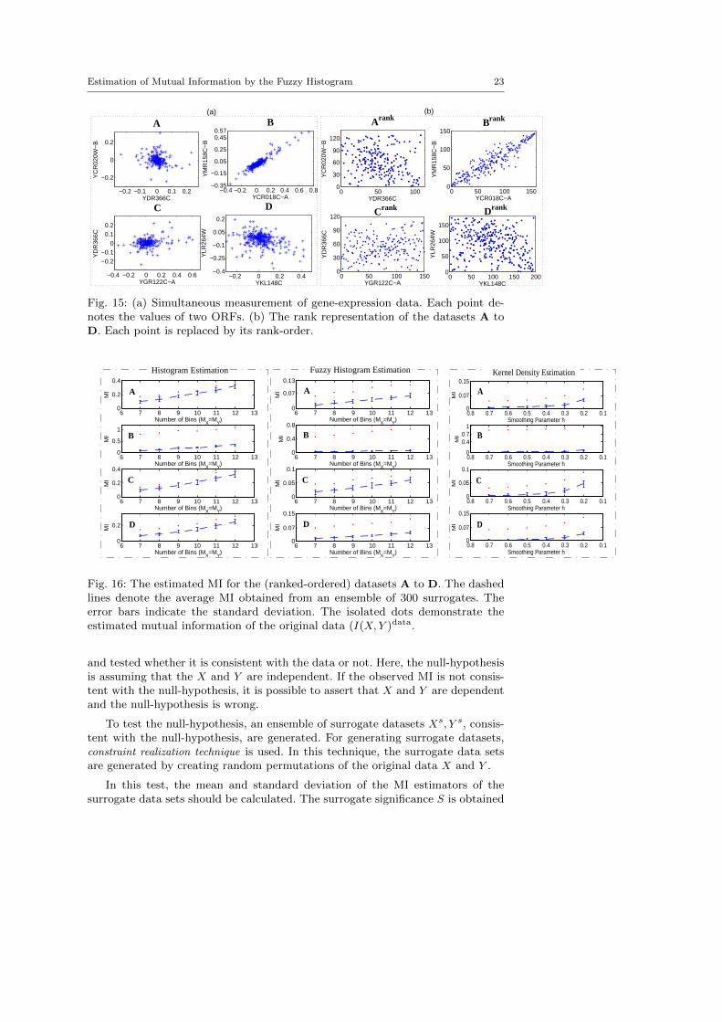
Fig. 16: The estimated MI for the (ranked-ordered) datasets A to D. The dashedlines denote the average MI obtained from an ensemble of 300 surrogates. Theerror bars indicate the standard deviation. The isolated dots demonstrate theestimated mutual information of the original data (I(X,Y )data.

and tested whether it is consistent with the data or not. Here, the null-hypothesisis assuming that the X and Y are independent. If the observed MI is not consis-tent with the null-hypothesis, it is possible to assert that X and Y are dependentand the null-hypothesis is wrong.

To test the null-hypothesis, an ensemble of surrogate datasets Xs, Y s, consis-tent with the null-hypothesis, are generated. For generating surrogate datasets,constraint realization technique is used. In this technique, the surrogate data setsare generated by creating random permutations of the original data X and Y .

In this test, the mean and standard deviation of the MI estimators of thesurrogate data sets should be calculated. The surrogate significance S is obtained


by:

S =I(X,Y )data −

⟨I(X,Y )

⟩surrogateσsurrogate

, (25)

where I(X,Y )data is the estimated MI of the original data, and⟨I(X,Y )

⟩surrogateis the average of the estimated MI for the ensemble of the surrogate datasets. If|S| ≥ 2.6, the null-hypothesis is rejected by a significant level of 99%.

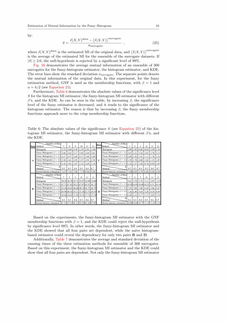
Fig. 16 demonstrates the average mutual information of an ensemble of 300surrogates for the fuzzy-histogram estimator, the histogram estimator, and KDE.The error bars show the standard deviation σsurrogate. The separate points denotethe mutual information of the original data. In this experiment, for the fuzzyestimation method, GNF is used as the membership functions, with β = 1 andα = h/2 (see Equation 23).

Furthermore, Table 6 demonstrates the absolute values of the significance levelS for the histogram MI estimator, the fuzzy-histogram MI estimator with differentβ’s, and the KDE. As can be seen in the table, by increasing β, the significancelevel of the fuzzy estimator is decreased, and it tends to the significance of thehistogram estimator. The reason is that by increasing β, the fuzzy membershipfunctions approach more to the crisp membership functions.

Table 6: The absolute values of the significance S (see Equation 25) of the his-togram MI estimator, the fuzzy-histogram MI estimator with different β’s, andthe KDE.

DataNumber of Bins

Method 7 8 9 10 11 12 Data

Number of BinsMethod 7 8 9 10 11 12

A

Histogram 3.73 2.08 2.38 1.55 2.01 1.90

C

Histogram 2.09 1.82 0.68 0.65 2.50 1.16

Fuzzy Histogram ( 1 ) 5.68 5.62 5.17 5.85 5.69 5.01 Fuzzy Histogram ( 1 ) 3.87 3.21 3.24 2.65 2.70 3.15




h Method 0.2 0.3 0.4 0.5 0.6 0.7

h Method 0.2 0.3 0.4 0.5 0.6 0.7

Kernel density estimation 6.57 7.14 7.06 7.74 8.84 9.48 Kernel density estimation 3.60 4.68 5.79 6.46 6.68 6.58

B

Number of Bins Method 7 8 9 10 11 12

Number of Bins

Method 7 8 9 10 11 12

Histogram 34.22 28.78 25.71 25.87 22.88 19.84

D

Histogram 5.61 3.70 3.75 3.11 2.95 2.35

Fuzzy Histogram ( 1 ) 67.71 67.42 58.12 67.87 65.53 56.72 Fuzzy Histogram ( 1 ) 10.9510.69 10.60 10.25 8.51 10.10




h Method 0.2 0.3 0.4 0.5 0.6 0.7

h Method 0.2 0.3 0.4 0.5 0.6 0.7

Kernel density estimation 41.19 47.51 58.31 59.35 63.36 67.95 Kernel density estimation 10.0210.64 10.77 11.19 11.6711.81

Based on the experiments, the fuzzy-histogram MI estimator with the GNFmembership functions with β = 1, and the KDE could reject the null-hypothesisby significance level 99%. In other words, the fuzzy-histogram MI estimator andthe KDE showed that all four pairs are dependent, while the naıve histogram-based estimator could reveal the dependency for only two pairs B and D.

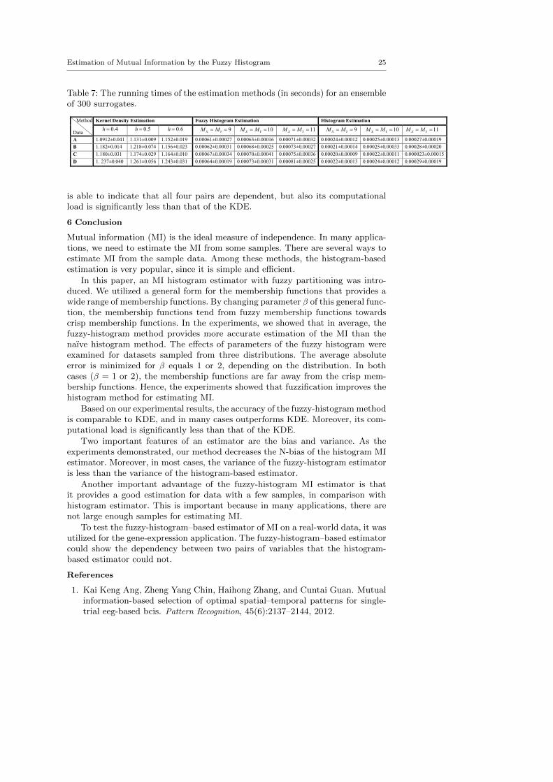
Additionally, Table 7 demonstrates the average and standard deviation of therunning times of the three estimation methods for ensemble of 300 surrogates.Based on this experiment, the fuzzy-histogram MI estimator and the KDE couldshow that all four pairs are dependent. Not only the fuzzy-histogram MI estimator


Table 7: The running times of the estimation methods (in seconds) for an ensembleof 300 surrogates.

In the new version of the paper the non-related references were eliminated, and currently the number of references has been reduced to 26 from 37.

We appreciate the comments from the reviewers. Thank you for reviewing our manuscript.

Sincerely,Maryam Amir Haeri and Mohammad Mehdi Ebadzadeh

Method Data

Kernel Density Estimation Fuzzy Histogram Estimation Histogram Estimation

0.4h 0.5h 0.6h 9X YM M 10X YM M 11X YM M 9X YM M 10X YM M 11X YM M

A 1.0912±0.041 1.131±0.009 1.152±0.019 0.00061±0.00027 0.00063±0.00016 0.00071±0.00032 0.00024±0.00012 0.00025±0.00013 0.00027±0.00019

B 1.182±0.014 1.218±0.074 1.156±0.023 0.00062±0.00031 0.00068±0.00025 0.00073±0.00027 0.00021±0.00014 0.00025±0.00033 0.00028±0.00020

C 1.180±0.031 1.174±0.029 1.164±0.010 0.00067±0.00034 0.00070±0.00041 0.00075±0.00036 0.00020±0.00009 0.00022±0.00011 0.000023±0.00015

D 1. 237±0.040 1.261±0.056 1.243±0.031 0.00064±0.00019 0.00073±0.00031 0.00081±0.00025 0.00022±0.00013 0.00024±0.00012 0.00029±0.00019

is able to indicate that all four pairs are dependent, but also its computationalload is significantly less than that of the KDE.

6 Conclusion

Mutual information (MI) is the ideal measure of independence. In many applica-tions, we need to estimate the MI from some samples. There are several ways toestimate MI from the sample data. Among these methods, the histogram-basedestimation is very popular, since it is simple and efficient.

In this paper, an MI histogram estimator with fuzzy partitioning was intro-duced. We utilized a general form for the membership functions that provides awide range of membership functions. By changing parameter β of this general func-tion, the membership functions tend from fuzzy membership functions towardscrisp membership functions. In the experiments, we showed that in average, thefuzzy-histogram method provides more accurate estimation of the MI than thenaıve histogram method. The effects of parameters of the fuzzy histogram wereexamined for datasets sampled from three distributions. The average absoluteerror is minimized for β equals 1 or 2, depending on the distribution. In bothcases (β = 1 or 2), the membership functions are far away from the crisp mem-bership functions. Hence, the experiments showed that fuzzification improves thehistogram method for estimating MI.

Based on our experimental results, the accuracy of the fuzzy-histogram methodis comparable to KDE, and in many cases outperforms KDE. Moreover, its com-putational load is significantly less than that of the KDE.

Two important features of an estimator are the bias and variance. As theexperiments demonstrated, our method decreases the N-bias of the histogram MIestimator. Moreover, in most cases, the variance of the fuzzy-histogram estimatoris less than the variance of the histogram-based estimator.

Another important advantage of the fuzzy-histogram MI estimator is thatit provides a good estimation for data with a few samples, in comparison withhistogram estimator. This is important because in many applications, there arenot large enough samples for estimating MI.

To test the fuzzy-histogram–based estimator of MI on a real-world data, it wasutilized for the gene-expression application. The fuzzy-histogram–based estimatorcould show the dependency between two pairs of variables that the histogram-based estimator could not.

References

1. Kai Keng Ang, Zheng Yang Chin, Haihong Zhang, and Cuntai Guan. Mutualinformation-based selection of optimal spatial–temporal patterns for single-trial eeg-based bcis. Pattern Recognition, 45(6):2137–2144, 2012.


2. J.F. Crouzet and O. Strauss. Interval-valued probability density estimationbased on quasi-continuous histograms: Proof of the conjecture. Fuzzy Sets and

Systems, 183(1):92–100, 2011.3. G. Darbellay. Entropy expressions for multivariate continuous distributions.

IEEE Transactions on Information Theory, 46(2):709–712, 2000.4. G.A. Darbellay and I. Vajda. Estimation of the information by an adaptive

partitioning of the observation space. Information Theory, IEEE Transactions

on, 45(4):1315–1321, 1999.5. T.R. Hughes. Supplementary data file of gene expression. http://hugheslab.

ccbr.utoronto.ca/supplementary-data/rii/. [Online; accessed 20-December-2012].

6. T.R. Hughes, M.J. Marton, A.R. Jones, C.J. Roberts, R. Stoughton, C.D.Armour, H.A. Bennett, E. Coffey, H. Dai, Y.D. He, et al. Functional discoveryvia a compendium of expression profiles. Cell, 102(1):109–126, 2000.

7. Masayuki Karasuyama and Masashi Sugiyama. Canonical dependency anal-ysis based on squared-loss mutual information. Neural Netw., 34:46–55, 2012.

8. A. Kraskov, H. Stogbauer, and P. Grassberger. Estimating mutual informa-tion. Physical Review E, 69(6):066138, 2004.

9. Kevin Loquin and Olivier Strauss. Fuzzy histograms and density estimation.In Jonathan Lawry, Enrique Miranda, Alberto Bugarin, Shoumei Li, Mari-aAngeles Gil, Przemys aw Grzegorzewski, and Olgierd Hyrniewicz, editors,Soft Methods for Integrated Uncertainty Modelling, volume 37 of Advances in

Soft Computing, pages 45–52. Springer Berlin Heidelberg, 2006.10. Kevin Loquin and Olivier Strauss. Histogram density estimators based upon

a fuzzy partition. Statistics and Probability Letters, 78(13):1863 – 1868, 2008.11. R. Moddemeijer. On estimation of entropy and mutual information of con-

tinuous distributions. Signal Processing, 16(3):233 – 248, 1989.12. Y.I. Moon, B. Rajagopalan, and U. Lall. Estimation of mutual information

using kernel density estimators. Physical Review E, 52(3):2318–2321, 1995.13. E. Schaffernicht, R. Kaltenhaeuser, S. Verma, and H.M. Gross. On estimating

mutual information for feature selection. Artificial Neural Networks–ICANN

2010, pages 362–367, 2010.14. R. Steuer, J. Kurths, C.O. Daub, J. Weise, and J. Selbig. The mutual informa-

tion: detecting and evaluating dependencies between variables. Bioinformatics,18(suppl 2):S231–S240, 2002.

15. Kiril Tenekedjiev and Natalia Nikolova. Justification and numerical real-ization of the uniform method for finding point estimates of interval elicitedscaling constants. Fuzzy Optimization and Decision Making, 7(2):119–145, 2008.

16. Qiang Wang, Yi Shen, and Jian Qiu Zhang. A nonlinear correlation measurefor multivariable data set. Physica D: Nonlinear Phenomena, 200(3-4):287 –295, 2005.

17. K. Zografos and S. Nadarajah. Expressions for renyi and shannon entropies formultivariate distributions. Statistics & Probability Letters, 71(1):71–84, 2005.

http://hugheslab.ccbr.utoronto.ca/supplementary-data/rii/

http://hugheslab.ccbr.utoronto.ca/supplementary-data/rii/

Documents

Estimation of Mutual Information by the Fuzzy Histogram · The integrals of theEquation 3measure the smoothness of the probability density functions. When the pdf’s are smooth,