Embed Size (px)
Citation preview

ESTIMATION OF NET CARBON SEQUESTRATION POTENTIAL OF
CITRUS UNDER DIFFERENT MANAGEMENT SYSTEMS USING THE LIFE
CYCLE APPROACH
BY
JACKSON MWAMBA BWALYA
A DISSERTATION SUBMITTED TO THE UNIVERSITY OF ZAMBIA IN PARTIAL
FULFILLMENT OF THE REQUIREMENTS FOR THE AWARD OF THE DEGREE
OF MASTER OF SCIENCE IN AGRONOMY
THE UNIVERSITY OF ZAMBIA
LUSAKA
2012

i
DECLARATION
I, Jackson Mwamba Bwalya, declare that this dissertation represents a genuine research I
carried out and that no part of this dissertation has been submitted for any other degree
or diploma at this or another university or institution.
……………………………… ………………………...………..
Signature Date

ii
APPROVAL FORM
This dissertation of Mr. Jackson Mwamba Bwalya is approved as fulfilling part of the
requirements for the award of the degree of Master of Science in agronomy (Plant
Science) of the University of Zambia.
Name and Signature of Examiners
Internal Examiners
1. Name: …………………………Signature: …………………..Date: …………………
2. Name: ……….…………………Signature: …………………..Date: …………………
3. Name: …………………………Signature: …………………..Date: …………………

iii
DEDICATION
I dedicate this dissertation to my daughter, Chewe Bwalya, and my parents; Mr. Lackson
Mwamba and Ms. Veronica Chewe and my siblings.

iv
ABSTRACT
A study was conducted to determine the net carbon sequestration potential of citrus to
mitigate climate change. Perennial crops such as citrus have the potential to absorb and
sequester carbon dioxide from the atmosphere, save for the carbon released back through
the application of agro-chemical inputs and use of fossil fuels in running farm machinery
in the management of citrus production systems. The main objective of this study was to
determine the net carbon sequestration potential of sweet orange (Citrus sinensis (L.)
Osbeck), orchards under different management systems. The biomass densities and the
carbon stocks (carbon sequestration) of citrus trees were determined and orchard carbon
emissions estimated and converted to carbon equivalents. Carbon stocks were estimated
using standard carbon inventory methods. Allometric equations were used to transform
citrus tree diameter into biomass. Farmers from the ten fields used in this study analysis
were asked over input application history to the orchards. Life cycle assessment based
carbon foot-printing methods were used to determine citrus orchard carbon emissions.
The carbon emission factors were calculated in conformity with PAS 2050. Results
obtained showed that citrus trees carbon sequestration in biomass ranged from 23.99 Mg
CO2e/ha for young trees to 109 Mg CO2e/ha for mature trees.
The carbon emissions from fertilizer, pesticides, water, electricity and fuels production,
delivery and use was estimated to range from 0.22 Mg CO2e/ha for low input orchards to
4.28 Mg CO2e/ha for high input management. The net carbon sequestration potential
were calculated to be between 15.35 Mg CO2 eq/ha and 95.14 Mg CO2 eq/ha for input
application ranging from two years to 16 years. Continous application of agro-chemical
inputs beyond the optimum fruit bearing age could result in net carbon emissions and is
not justified. The carbon sequestered (biomass accumulation) in trees was observed to
increase with age (r2 = 0.55) and was not seen to increase directly with the increase in
carbon emissions (r2 = 0.44), but it was apparent that increase in inputs especially
fertilizer, pesticides and electricity resulted in increased greenhouse gas emissions. An
opportunity exist in the growing of citrus especially with low input management and
under well managed high input management systems to mitigate climate change by
reducing CO2 from the atmosphere through carbon sequestration in citrus biomass.

v
ACKNOWLEDGEMENTS
I wish to avail my gratitude to Dr. Mebelo Mataa of Plants Science Department of the
University of Zambia and Mr. Daud Kachamba of Bunda College of the University of
Malawi, for their expert guidance and counsel from the time of developing a research
concept and writing a research proposal and through implementation to reporting of the
results by writing this dissertation and submission.
I am also elated to Mr. Yobe Nyirenda, a Senior GIS Technician of the Forest
Department for assisting with the forestry inventory tools and equipment and in the
actual data collection. It was not an easy task going round orchards scattered all over
Lusaka collecting data. It required determination and dedication, that which can only be
achieved with a selfless heart.
I am deeply indebted to Dr. Masuwa of the Ministry of Agriculture and Livestock head
office and Mr. Pascal Chipasha at the Lusaka Provincial office for the assistance in the
identification of the citrus farmers in Lusaka province. In the same vein I would like to
thank all the agricultural extension officers of Lusaka province, with whom I worked on
this study.
I acknowledge with thanks the financial and moral support I received from my
employer, the Ministry of Agriculture and Livestock, North Western provincial office at
Solwezi. In this regard I wish to thank Mr. Charles Sondashi; the Provincial Agricultural
Coordinator, Mr. Amos Malumo; the Principal Agricultural Officer and the Provincial
Accounts staff for having facilitated my studies. I wish also to thank all my workmates
for moral support.
Lastly, but not the least, I wish to extend my appreciation to all my course mates. In a
way unimaginable to each one of them individually and as a group, I unbelievably
enjoyed their company and I derived a lot of encouragement to work hard.

vi
Table of Contents
ABSTRACT ................................................................................................................................... iv
ACKNOWLEDGEMENTS ............................................................................................................ v
LIST OF TABLES ......................................................................................................................... ix
LIST OF FIGURES ...................................................................................................................... xii
Chapter 1 ......................................................................................................................................... 1
1.0 INTRODUCTION ................................................................................................................ 1
Chapter 2 ......................................................................................................................................... 4
2.0 LITERATURE REVIEW ..................................................................................................... 4
2.1Global Climate Change ...................................................................................................... 4
2.2 Biomass and assessment ................................................................................................... 6
2.3 Botanical characterization of citrus ................................................................................... 8
2.4 Life cycle assessment method of assessing environmental impact ................................... 9
2.5 Carbon emission associated with agricultural inputs .......................................................... 11
2.5.1 Fuel and electricity ....................................................................................................... 11
2.5.2 Chemical fertilizers ...................................................................................................... 12
2.5.3 Pesticides ...................................................................................................................... 12
Chapter 3 ....................................................................................................................................... 14
3.1 MATERIALS and METHODS ........................................................................................... 14
3.1.1 Biomass determination ................................................................................................. 17
3.1.2 System boundary .......................................................................................................... 19
3.2.1 Biomass determination (carbon sequestration) ............................................................ 20
3.2.2 LCA BASED CARBON FOOTPRINTS OF ORCHARDS ........................................ 23
Chapter 4 ....................................................................................................................................... 36
4.0 RESULTS ........................................................................................................................... 36
4.1 BIOMASS DETERMINATION: HIGH-INPUT ORCHARD SYSTEMS .................... 36
4.1.1 Biomass Determination (Carbon sequestration) for Plot 1 in Kafue district ............... 36
4.1.2 Biomass (Carbon sequestration) of citrus trees in Plot 2 in Kafue district .................. 38

vii
4.1.3 Biomass (Carbon sequestration) results in Plot 3 in Kafue district ............................. 38
4.1.4 Biomass (Carbon sequestration) of Plot 4 in Kafue district ......................................... 39
4.1.5 Biomass (Carbon sequestration) of Plot 5 in Kafue district ......................................... 41
4.2.1 Biomass (Carbon sequestration) of Plot 6 in Lusaka district ....................................... 42
4.2.2 Biomass (Carbon sequestration) of Plot 7 in Kafue district ......................................... 44
4.2.3 Biomass (Carbon sequestration) of Plot 8 in Kafue district ......................................... 46
4.2.4 Biomass (Carbon sequestration) of Plot 9 in Palabana area of Chongwe
district .................................................................................................................................... 48
4.2.5 Biomass (Carbon sequestration) of Plot 10 of Chikupi area of Kafue district ............ 50
4.3.1 Regression Analysis ..................................................................................................... 52
4.3.2 Biomass Analysis ......................................................................................................... 52
4.4 HIGH INPUT ORCHARDS ........................................................................................... 53
4.4.1 Emission for High input Plots ...................................................................................... 53
4.4.2 Emissions determination for Plot 6 orchard ................................................................. 66
4.4.3 Emissions determination for Plot 7 orchard ................................................................. 67
4.4.4 Emissions determination for Plot 8 orchard ................................................................. 69
4.4.5 Carbon emissions determination for Plot 9 orchard ..................................................... 71
4.4.6 Carbon emissions determination for Plot 10 Orchard .................................................. 72
4.8 SUMMARY OF GHG EMISSIONS .............................................................................. 76
Chapter 5 ....................................................................................................................................... 83
DISCUSSION ........................................................................................................................... 83
Carbon sequestration ............................................................................................................. 83
Life cycle assessment ............................................................................................................ 85
Net carbon sequestration ....................................................................................................... 88
Chapter 6 ....................................................................................................................................... 90
6.0 CONCLUSIONS AND RECOMMENDATIONS ............................................................. 90
6.1 Conclusion ...................................................................................................................... 90
6.2 Recommendations ........................................................................................................... 91
Chapter 7 ....................................................................................................................................... 92
REFERENCES .............................................................................................................................. 92

viii
APPENDICES .............................................................................................................................. 99
APPENDIX A ........................................................................................................................... 99
APPENDIX B ......................................................................................................................... 109
APPENDIX C ......................................................................................................................... 111

ix
LIST OF TABLES
Table 1: Location of the study plots within Lusaka Province ....................................................... 16
Table 2: Allometric equations for the calculations of aboveground biomass ............................... 18
Table 3: Carbon stock and sequestration results for citrus trees in Plot 1 determined
using four different allometric equations ...................................................................................... 37
Table 4: Plot 2 carbon stock and sequestration results ................................................................. 38
Table 5: Carbon stock and sequestration Results for Plot 3 in Kafue district ............................... 39
Table 6: Biomass (carbon sequestration) results for Plot 4 in Kafue district ................................ 40
Table 7: Carbon stock and sequestration results for plot 5 ........................................................... 41
Table 8: Summary of carbon stock and sequestration results for the five high input
orchards ......................................................................................................................................... 42
Table 9: Carbon stock and sequestration results for Plot 6 in Lusaka district .............................. 43
Table 10: Plot 7 carbon stock and sequestration results ............................................................... 45
Table 11: Carbon stock and sequestration results for Plot 8 in Chikupi area of Kafue
district ............................................................................................................................................ 47
Table 12: Carbon stock and sequestration results for Plot 9 in Palabana-Chongwe district ......... 49
Table 13: Carbon stock and sequestration results for Plot 10 in Kafue district ............................ 51
Table 14: Average carbon sequestration results for four low input orchards ............................... 51
Table 15: Summary of regression analysis results for DBH against biomass
accumulation ................................................................................................................................. 52
Table 16: Summary carbon sequestration results from ten orchards ............................................ 52
Table 17: Initial land preparation equipment and fuel consumption per ha ................................. 55
Table 18: Land maintenance equipment and fuel consumption per ha. Land maintenance
was performed after old or unproductive trees were removed in readiness to plant new
ones. .............................................................................................................................................. 55
Table 19: Direct GHG emissions from burning of fossil fuel in the operation of tractor
for initial land preparations ........................................................................................................... 55
Table 20: Volatile organic carbon and carbon monoxide emissions from tractor exhaust
during initial land preparation activities ....................................................................................... 56

x
Table 21: Volatile organic carbon and carbon monoxide exhaust emissions from tractor
during land maintenance activities in preparation for tree replacement ....................................... 56
Table 22: Emission factors due to burning of dry matter of citrus trees removed due to
old age and low productivity. Four percent of biomass per ha is replaced annually. ................... 56
Table 23: Spreading of GHG emissions from initial land preparations at two and half
percent per annum and emissions from the burning of biomass and land maintenance
were amortized at the rate of four percent per annum. ................................................................. 57
Table 24: Equipment used in orchards for cultural practices of mowing, spraying and
mechanical fertilizer application and their respective fuel consumption in the
management of citrus orchards used in the study. ........................................................................ 57
Table 25: Emissions from fuels used in orchard management practices ...................................... 58
Table 26: Volatile organic carbon and carbon monoxide exhaust emissions from tractor
used in tending activities of spraying, fertilizer application and mowing of weeds. .................... 58
Table 27: Energy consumption from pumping water for irrigation was calculated from
equation 18. Water was pumped into a reservoir from which it was made to flow by
gravity to individual citrus trees. ................................................................................................... 58
Table 28: Upstream energy expended in production of electricity and fuels ............................... 59
Table 29: Upstream GHG emissions arising from production of fuels and electricity that
were used in the orchard management .......................................................................................... 59
Table 30: Emissions of volatile organic carbon and carbon monoxide from production of
electricity and diesel ...................................................................................................................... 59
Table 31: Agro-chemical inputs (fertilizer and insecticides) orchard management ..................... 60
Table 32: Upstream energy inputs for the production, transportation, packaging and
application of fertilizers ................................................................................................................ 60
Table 33: Emissions from production of fertilizer used in orchard management ......................... 61
Table 34: Volatile organic carbon (VOC) and carbon monoxide (CO) emissions from
fertilizer production ....................................................................................................................... 61
Table 35: Energy requirements for the production, formulation, packaging and
distribution of pesticides ............................................................................................................... 62
Table 36: Emissions factors and GHG emissions from production of pesticides; emission
factors were multiplied by the energy used in the production of pesticides. ................................ 63

xi
Table 37: Volatile organic carbon (VOC) and carbon monoxide (CO) emissions from
production of pesticides ................................................................................................................ 64
Table 38: Summary of carbon dioxide equivalent emissions for Plot 1; after conversion
of LCA data to carbon equivalents using the respective global warming potential...................... 65
Table 39: Summary of GHG emissions in for the five high-input orchards ................................. 66
Table 40: The agro-chemical input (fertilizer and pesticides) to the orchard ............................... 67
Table 41: Summary of GHGs emissions for Plot 6 in Lusaka district .......................................... 67
Table 42: Agro-chemical inputs to the orchard............................................................................. 68
Table 43: Summary of GHG emissions for Plot 7 orchard ........................................................... 69
Table 44: Agro-chemical inputs to the orchard............................................................................. 70
Table 45: Summary of GHGs emissions for Plot 8 ...................................................................... 70
Table 46: Agro-chemical inputs to Plot 9 orchard ........................................................................ 71
Table 47: Summary of GHGs emissions for Plot 9 Orchard ........................................................ 72
Table 48: Agro-chemical inputs to Plot 10 ................................................................................... 73
Table 49: Summary of GHG emissions for Plot 10 Orchard ........................................................ 73
Table 50: Summary of carbon emissions for the four (4) low input orchards .............................. 74
Table 51: Weighted average accumulated emissions from the low input orchards ..................... 75
Table 52: Summary of carbon emissions for the ten orchards ...................................................... 76
Table 53: Summary of carbon sequestration, GHG emissions and net carbon
sequestration for the ten orchards ................................................................................................. 77
Table 54: Average carbon sequestration results for different levels of management ................... 78
Table 55: Average GHG emissions for different levels of management ...................................... 79
Table 56: Net carbon sequestration potential of orchard per management level .......................... 79

xii
LIST OF FIGURES
Figure 1: Map of the Republic of Zambia showing Lusaka Province .......................................... 15
Figure 2: Study area-Map of Lusaka Province showing the distribution of the plots from
the selected orchards. .................................................................................................................... 16
Figure 3: Systems boundary concept (Source: EPA, 2010). ......................................................... 20
Figure 4: Picture of a high-input citrus orchard (Plot 1) in Kafue district .................................... 37
Figure 5: Picture of a commercial (high-input) orchard (Plot 4) in Kafue district ....................... 40
Figure 6: Picture showing small holder orchard (Plot 6) in Lusaka district ................................. 43
Figure 7: Picture showing low-input orchard (Plot 7) in Chikupi area of Kafue district.............. 45
Figure 8: Picture showing citrus trees in a Low input orchard (Plot 8) in Kafue district ............. 47
Figure 9: Six year old small holder orchard (Plot 9) in Palabana of Chongwe district ................ 49
Figure 10: Picture of Low input orchard (Plot 10) in Kafue district ............................................. 50
Figure 11: Biomass and carbon sequestration, with annual CO2e increment in citrus
orchards ......................................................................................................................................... 53
Figure 12: Average carbon sequestration and emissions by management level ........................... 75
Figure 13: Total GHG emissions for the ten orchards in various districts of Lusaka
province ......................................................................................................................................... 77
Figure 14: Carbon sequestration, GHG emissions and net carbon sequestration. Carbon
emissions were indicated as negative (middle bar) and the carbon sequestration was
denoted by positive values. The net carbon sequestration was the difference between
carbon sequestration and carbon emissions (right bar) were positive for all the ten (10)
orchards. ........................................................................................................................................ 78
Figure 15: Net carbon sequestration by management level. The average carbon
sequestration for high input (left bar) orchards is lower than that for low inputs. Net
carbon sequestration for both management levels was postive and there was higher
average net carbon sequestration for low input orchards than for the high input orchards. ......... 80
Figure 16: The average distribution of carbon emissions by contribution per activity
under high (a) and low (b and c) in-puts systems showing the differences of contribution
of fertilizer production and application to total GHG emissions between high and low
input orchard management. ........................................................................................................... 81

xiii
Figure 17: Emissions distribution by activity-low input (d to f) orchards. For low input
orchards where fertilizer application is low, the contribution of GHG emissions from
fertilizer production and application is also low. .......................................................................... 82

xiv
LIST OF ACRONYMS
CDM: Clean Development Mechanism
CO: Carbon monoxide
DBH: Diameter at breast height (30 cm aboveground in this case)
EPA: US Environmental Protection Agency
FAO: Food and Agriculture Organization
GHG: Greenhouse gases
GREET: Greenhouse Gases Regulated Emissions, Energy and Transportation
GWP: Global warming potential
ha: Hectare
IPCC: Intergovernmental Panel on Climate Change
ISO: International Standards Organization
LCA: Life cycle assessment
LHV: Lower heating value
MACO: Ministry of Agriculture and Cooperatives
MAL: Ministry of Agriculture and Livestock
MMBTU: 106 British thermal unit (10
6 Btu)
PAS: Publicly available specifications
UNEP: United Nations Environmental Programme
UNFCCC: United Nations Framework Convention on Climate Change
VOC: Volatile Organic Carbon
WMO: World Meteorological Organization

1
Chapter 1
1.0 INTRODUCTION
The emergence of extreme weather changes as result of climate change is expected to
have great impact on plant development. The increase in global temperatures will result
in higher water holding capacity of the atmosphere with precipitation expected to
increase, (IPCC, 2001). However, potential evapo-transpiration is expected to exceed the
summer precipitation with an increased frequency in droughts. The potential impacts of
climate change on agriculture will be reflected most directly through the response of
crops, soils, weeds, insects and diseases to the elements of climate to which they are
most sensitive. Many weeds as well as plants are expected to benefit from increased
carbon dioxide concentration through enhanced photosynthesis. Insect pests, fungal and
bacterial pathogens of importance to agriculture production are sensitive to the effects of
the changes in moisture and temperatures on the host susceptibility and the host-parasite
inter-relations.
Climate Changes especially that involving high frequency in extreme events such as
droughts, , flooding, storms and heat waves will impact negatively on the agricultural
dependent rural livelihoods, threatening agricultural production systems that ensure
food security and income generation, (Bockel et al., 2011).
Agriculture is a major source of GHG, contributing about 20 percent of total global
emissions which rises to over 30 percent when combined with related changes in land
use including deforestation; mainly driven by the expansion of agricultural lands, (Cole
et al., 1997). Other causes of the increase in GHG concentration in the atmosphere
include natural causes such as volcanic activity and changes in the composition of the
earth’s atmosphere. The high mitigation potential for climate change lies with
agricultural sector in developing countries. The technical mitigation options available
from agriculture, forestry and other land uses include reducing emissions of carbon
dioxide through the reduction of the rate of deforestation and forest degradation. This
could be through the adoption of improved cropland management practices (including

2
reduced tillage, integrated nutrient and water management and conservation agriculture);
reducing emissions of methane and nitrous oxide through improved manure and crop
residue management and more efficient management of irrigation water on rice paddies.
Further, improved synthetic fertilizer production and management and sequestering
carbon (C) through conservation farming practices, improved forest management
practices, afforestation and reforestation, agro-forestry; the growing of perennial tree
crops, (Bockel et al., 2011) are some of methods available for mitigation.
Citrus production is primarily an agricultural activity that is used to generate income for
producers through the production and sale of fruits. However, given the amount of
carbon dioxide that the trees fix through the plant dry matter it can play a role as a
means of removing carbon from the atmosphere –commonly referred to as carbon
sequestration. The amount of carbon dioxide removed from the atmosphere through
sequestration is proportionate to the amount of biomass the plant accumulates over its
life time, (Juwarkar et al., 2011). However, the growing of citrus, like all other crops, as
noted below requires additional external inputs which in turn release carbon dioxide to
the atmosphere and therefore the ultimate value of such systems as a sequestration
strategy will depend on whether the amount of carbon fixed exceeds that amount
generated through establishing and maintaining these trees.
The application of agro- inputs do not only cost farmers money, but also cost the
environment through an increase in greenhouse gases which eventually results in
increased temperatures.
Trees just like other plants are able to capture and fix carbon dioxide through the process
of photosynthesis. Carbohydrates may temporarily be stored by plants in the form of
sugars and polysaccharides such as starch and are permanently stored as cellulose and
lignin which act as structural components of plant. The amount of carbon dioxide
captured and fixed through the process of photosynthesis and stored by plants as
structural components can be estimated from the amount of dry biomass produced by the
plant. On the other hand the amount of carbon dioxide and other greenhouse gases

3
released as a result of the application of external inputs by the farmers to the citrus trees
can be determined by calculating the life cycle carbon footprint of each input.
Statement of the Problem
There is scientific empirical evidence that the concentrations of greenhouse gases are
rising and that agriculture contributes about 20% of global emissions, (Cole et al., 1997
and Marble et al., 2011). Agriculture has also potential to contribute to carbon
sequestration, especially through the growing of perennial crops such as oranges which
produce large aboveground biomass. The net outcome regarding carbon emissions and
sequestration in perennial plants is unknown and may differ depending on plant species,
geographical location, level of management and utilization of external inputs.
Objectives
The main objective of the study was to determine the net carbon sequestration of orange
(Citrus sinensis (L.) Osbeck) orchards under different management systems in Zambia.
Specific Objectives
� To determine the amount of carbon sequestered as biomass (above ground) under
different management systems.
� To estimate the greenhouse gas emissions during production
Justification of study
The findings from this study will contribute to elucidating the relationship between
carbon fluxes, orchard management systems and the effects on green house gases. This
may assist in accessing opportunities for carbon trading, contribute to the development
of sustainable agro-based community technologies to manage greenhouse gas emissions
and global warming.
4
Chapter 2
2.0 LITERATURE REVIEW
2.1Global Climate Change
Climate change refers to any significant shift or variability in temperature, precipitation,
humidity, light or wind. These changes can be of short or long duration covering
decades or longer (IPCC, 2007). Notwithstanding the fact that climate is dynamic and
has been changing through the ages, the recent emergence of extreme weather patterns is
attributed to anthropogenic activities including burning of fossil fuels for transport,
industrial practices, deforestation and agricultural activities.
The earth’s atmosphere contains carbon dioxide (CO2) and other green house gases such
as methane (CH4), nitrous oxide (N2O) that act as a heat insulation layer resulting in
progressive heat conservation by the atmosphere. This phenomenon results in the
retention of heat that is critical for maintaining habitable temperatures, causing the
planet to be warmer than it would otherwise been. There is irrefutable scientific
evidence that the concentration of the three most important greenhouse gasses (carbon
dioxide, methane and nitrous oxide) in the atmosphere have been increasing causing the
temperature at the Earth’s surface to rise, (IPCC, 2007). Fossil fuel combustion and land
use change including deforestation, soil organic carbon emissions, biomass burning and
drainage of wetlands have resulted in increased carbon emissions (IPCC, 2007). There
are suggestions that global surface air temperature may increase by 1.4 oC to 5.8
oC at
the end of the century (IPCC, 2001). The increase in surface air temperature level is
more directly linked to the increase in the concentration of CO2 in the atmosphere. The
risk is that increasing global temperatures could negatively affect biological systems,
(Lal, 2004). Higher temperatures may also cause higher sea levels due to melting of
polar icecaps thereby disrupting the marine and fresh water ecosystems, increase heat
related diseases, change rainfall patterns and increase the geographical spread of disease
vectors, insect pests and invasive weeds, (IPCC, 2001; Douglas, 2004). The effect of
rising temperature on agriculture could be more devastating. Shifts in precipitation and
5
temperatures may hinder some cropping patterns while at the same time benefiting
others. With rising global human population, any reduction in crop production due to
rainfall or temperature pattern induced reduced yield or disease or pest attack could have
devastating effect on food insecure families.
These potential impacts have raised concerns over potential global climate change with
the international organizations and nations. The World Climate Conference organized by
World Meteorological Organization (WMO) in 1979 led to the establishment of the
Intergovernmental Panel on Climate Change (IPCC) in 1988. Four years later, an
international environmental treaty, called United Nations Framework Convention on
Climate Change (UNFCCC), was formulated with the objective of reducing global
greenhouse gas emissions. The UNFCCC’s Kyoto Protocol, (UN, 1998) formulated in
1997 stimulated the amount of emission reduction by industrialized nations and
recognized forests or vegetative growth as carbon sequestration or potential carbon
storage (Brown, 2002).
The agriculture sector is one of the largest contributors to carbon emissions behind
energy production (Johnson et al., 2007). Emissions from agriculture account for an
estimated 20 per cent of the annual increase in global GHG emissions. When land use
change involving deforestation or clearing of land for agricultural expansion, soil
degradation and biomass burning, the agriculture contribution to emissions is raised to
one-third of all anthropogenic emissions, (Cole et al., 1997). The biggest contribution to
the increase in carbon dioxide concentration comes from burning of fossil fuel, but
agriculture also contributes significantly from biomass burning and other land use
changes. Agriculture is considered a major contributor of methane and nitrous oxide,
(Cole et al., 1997). Methane is emitted from flooded rice fields, wet lands and from
animal raring. The major source of nitrous oxide emissions is the large scale production
and application of inorganic nitrogen fertilizers. A lot of studies have been focused on
reducing the emissions from agriculture, (Cole et al., 1997; Lal et al., 1998 and Lal,
2004). However, it is believed that emission reduction alone will not be sufficient to
curtail the impacts on the environment and therefore long term carbon sequestration is
necessary.

6
Carbon sequestration involves the capture and storage of carbon dioxide produced by
burning of fossil fuels and other anthropogenic activities from the atmosphere and
storing it away in long-lived carbon pools, (Nair et al., 2009). Some of the potential
carbon storage sites include depleted oil fields, sedimentary rocks and injecting carbon
dioxide in the sediments below the ocean and that dissolved in the oceans. The other
method is through the terrestrial biological plant carbon sequestration; above-ground
plant biomass and below-ground biomass such as roots. Plants use energy from the
sunlight to convert carbon dioxide from the atmosphere to carbohydrates for their
growth and maintenance, via the process of photosynthesis. Plants being autotrophs are
able to absorb light energy and carbon dioxide. Carbon dioxide in the presence of light
and water is converted to glucose which is stored as carbohydrates. Carbohydrates are
stored as part of the body structure of the plant biomass in the form of cellulose, lignin
and other macromolecules (Losi et al., 2003 and Phat et al., 2004).
2.2 Biomass and assessment
The amount of carbon dioxide stored in a natural carbon sequestration infrastructure
such as photosynthesizing citrus biomass can be determined by measuring the amount of
biomass. Biomass has been defined as the organic material both above-ground and
below-ground, and both living and dead, such as citrus trees, crops, grasses, and others
(FAO, 2004a). The above-ground biomass consists of all living biomass above the soil
including stem, stump, branches, bark, seeds, and foliage. Below-ground biomass
consists of all living roots excluding fine roots (less than 2 mm in diameter). Biomass is
measured in fresh weight and dry weight. In carbon sequestration biomass is measured
as dry weight; Carbon is taken to account for 50% of dry weight, (Timothy et al., 2005;
Losi et al., 2003 and Juwarkar et al 2011; IPCC, 2005).
Many biomass assessment studies conducted focused on determining the above-ground
biomass in natural forest by use of allometric equations, (Juwarkar et al., 2011;
Adhikari, 2005; Brown, 1997; Brown et al., 1989; Vermer and de Meer, 2010; Phat et
al., 2004; Lasco et al., 2008; Segura and Kanninen, 2005; and Zemeck, 2009) and by use

7
of remote sensing, (Torio, 2007). Some studies have also been carried out aimed at
estimating and modeling carbon sequestration in aforestation, agro-forestry and forest
management, (Hairiah et al., 2001 and Masera et al., 2003), with other crop specific
studies such as Cocoa (Theobroma cacao), (Isaac et al., 2007) and coffee (Shorea
javanica), (Noordwijk et al., 2002). Allometric equations have been used in the
determination of aboveground biomass of natural forest tree species and these equations
relate biophysical properties such as diameter at breast height (DBH) and height to
biomass, (Brown, 1997; de Gier, 1999; Ketterings et al, 2001; de Gier, 2003 and Zianis
and Mencuccini, 2004). Few studies have focused on carbon sequestration in orchards,
(Page, 2011 and Marble et al., 2011). Morgan et al, (2006) did a study to determine
nitrogen and biomass accumulation in citrus (Citrus sinensis (L.)) using the destructive
method of biomass determination. Orchard species have higher growth rates and thus
accumulates large amount of carbon in the first stage, (14-20 years) of their life span
(Manner et al., 2006) after which they virtually stop growing. On the other hand natural
forest trees have higher specific gravity and are slower growing species which allows
them to accumulate more carbon in the long term. Natural forest trees are reported to
continue accumulating biomass over a longer period of time (Hairiah et al., 2001).
Biomass is an indicator of carbon sequestration and hence the need to determine the
biomass of perennial crops including citrus trees, mangoes and many other agro-forestry
trees.
The procedure employed in the determination of aboveground biomass is outlined in
Timothy et al (2005). The method involves randomly selecting sample trees, measuring
the growth variables (i.e. DBH or tree height) and relating these variables to tree
biomass.
There are two methods available for measuring sample tree biomass- these are the
destructive and non-destructive. The conventional destructive method is done by felling
the sample tree and then weighing it and this procedure is very laborious and costly. The
non-destructive method does not require the trees to be felled. Biomass is determined
from allometric equations that have been specifically developed for calculating biomass
for dry tropical forests (Brown, 1997) for citrus and agro-forestry shade trees (Schroth et

8
al., 2002) Andhra Pradesh Forest Department, (2010) and Segura et al., (2006) In this
study a non-destructive method was used to determine biomass.
2.3 Botanical characterization of citrus
The Citrus sinensis (L.) species is in the family of Rutaceae which belongs to the order
Sapindales in the Magnoliopsida and Magnoliophyta class and phylum respectively. The
other popular members of the family Rutaceae include mandarin (C. reticulata), grape
fruit (C. paradisi), lemons (C. limon) and the limes (C. aurantifolia), (Harley et al.,
2006). Common sweet orange varieties include the Washington Navel, Valencia Late,
Delta and Midnight. Others are the Pineapple, Bahianinha, Hamlin and Oasis
(FAO/MACO, 2007).
In Zambia, sweet oranges are grown as exotic evergreen medium sized trees. They are
cultivated under varied agro-ecological conditions ranging from dry hot regions (Region
I) to wetter subtropical regions (Region III). The water requirement range is from about
800 mm to 2000 mm per annum and they are commonly grown under irrigation in areas
with lower amount of rainfall. Citrus grow well between a temperature of 13 ºC and 37
ºC and can be grown in a wide range of soils ranging from sandy loam or alluvial soils to
clay loam or heavy clay soils (Manner et al., 2006). Citrus requires the external supply
of essential nutrients (N, P, K) and protection against pests and diseases and weeds
through the application of agro-chemical inputs. The supply of water is essential during
the drier part of the year.
The citrus growth rates are enhanced by application of fertilizers. Young trees in the
range of 5-10 years have higher growth rates. The optimum tree size is typically reached
between 10 and 14 years after transplanting and reaches peak fruit bearing age between
20 and 25 years. The citrus trees, however can survive up to 250 years for ornamental
trees (Manner et al., 2006). The application of agro- inputs do not only cost farmers
money, but also impact negatively on the environment by increasing greenhouse gases
which eventually results in increased ambient temperatures. It is postulated that increase
in global temperatures will result in higher water holding capacity of the atmosphere
with precipitation expected to change. The coastal areas are anticipated to experience

9
increase in rainfall, whereas other areas would record decline in annual rainfall.
Generally, potential evapo-transpiration is expected to exceed the summer precipitation
with an increased frequency in droughts (IPCC, 2001). The potential impacts of climate
change on agriculture will be reflected most directly through the response of crops, soils,
weeds, insects and diseases to the elements of climate to which they are most sensitive.
Many weeds as well as plants are expected to benefit from increased carbon dioxide
concentration through enhanced photosynthesis. Insect pests, fungal and bacterial
pathogens of importance to agriculture production are sensitive to the effects of the
changes in moisture and temperatures on the pest or pathogen, on the host susceptibility
and the host-parasite inter-relations as high moisture and temperatures favour the spread
of pests and diseases.
2.4 Life cycle assessment method of assessing environmental impact
Greenhouse gas emissions due to the application of agro-chemical inputs and the energy
use on the orchards can be assessed using carbon footprints based on life cycle
assessment methods. Life Cycle Assessment (LCA) is defined as a quantitative process
for evaluating the total environmental impact of a product over its entire life cycle,
referred to as a cradle to grave approach. LCA focuses on the product, with emphasis on
quantifying the environmental impacts (Heijungs, 1996). The LCA consists of four
phases; namely goal definition and scope, inventory analysis, impact assessment and
interpretation. The goal definition and scope phase includes identifying the product or
function to be studied, the reasons for carrying out the study, defining the system
boundary, and identifying the data requirements. Inventory analysis involves identifying
the process involved in the system, defining the inputs and outputs of each process, and
collecting data to quantify those inputs and outputs. Impact assessment defines impact
categories and uses the results of the inventory analysis to calculate indicator results in
those categories.
Finally, in the interpretation phase the results of the inventory analysis and impact
assessment are interpreted in terms of the goal and scope definition; the results are

10
checked for completeness, sensitivity, and consistency; and conclusions, limitations, and
recommendations are reported (ISO, 1997). Further LCAs generally fall into two
categories based on their purpose, that is, attributable and consequential LCAs. The
former is focused on looking back on a product and determining what emissions can be
attributed to it while the latter is directed on the environmental effects of what will
happen due to a decrease or increase in demands for goods and services (Ekvall and
Weidema, 2004).
Carbon Footprint is a measure of the exclusive total amount of carbon dioxide (CO2) and
other Greenhouse Gas (GHG) emissions that is directly and indirectly caused by an
activity or is accumulated over the life stages of a product and is usually expressed in
kilograms of CO2 equivalents, which may account for different global warming effects
by different Greenhouse Gases. Carbon Trust (2007) also broadly defines Carbon
Footprint as a methodology to estimate the total emission of greenhouse gases (GHG) in
carbon equivalents from a product across its life cycle from the production of raw
material used in its manufacture, to disposal of the finished product (excluding in-use
emissions). Its also defined as a technique for identifying and measuring the individual
greenhouse gas emissions from each activity within a supply chain process step and the
framework for attributing, these to each output product. The greatest challenge facing
sustainability of ecosystems and therefore human kind is the emissions of the major
green house gases; Methane (CH4), Nitrous oxide (N2O) and Carbon Dioxide (CO2) in
the atmosphere (Millennium Ecosystem Assessment, 2005 and Watson et al., 1998)
which have different global warming potential. A Global Warming Potential (GWP) is
an indicator that reflects the relative effect of a greenhouse gas in terms of climate
change when a fixed time period, such as 100 years is considered (IPCC, 2007).
A number of studies have been conducted that aimed at modeling energy and material
flows in citrus orchard production systems (Ozkan et al., 2003; Dalgaard et al., 2001 and
Namdari et al., 2011). Other studies have focused on carbon emissions from farm
operations with emphasis on tillage operations and the associated emissions reductions
from conventional tillage to zero tillage (Lal, 2004 and West and Marland, 2002).
Studies conducted using the life cycle assessment approach include that of Wood and

11
Cowie (2004) which gave the emission factors associated with the production of
chemical fertilizers-N, P2O5 and K2O. Life cycle assessment based carbon foot-printing
of orchards have also been done by researchers with a focus on Kiwifruits and apples
(Page, 2011), from which lessons were drawn during this study.
The emissions from inputs included the energy in the acquisition and use of agro-
chemical inputs and the use of farm machinery and equipment. This includes the use of
fossil fuels for running of tractors, electricity for running of water pumps and the
emission due to the manufacture, packaging, transportation and use of inorganic
fertilizers and pesticides. LCA approach has been used to calculate carbon footprints of
sugar cane in Zambia (Plassmann, 2010).
2.5 Carbon emission associated with agricultural inputs
2.5.1 Fuel and electricity
The use of fossil fuels in agriculture results in CO2 emissions from the combustion of the
fuels and the additional emission associated with the production and delivery of fuels to
the farm (West and Marland, 2002). Carbon emissions due to burning of fossil fuels are
estimated using carbon emission coefficients. Carbon dioxide emissions attributable to
electricity consumption are based on the fuels or energy used in power generation. The
Carbon dioxide emissions are determined per kilo watt-hour (kWh) of electricity
generated, transformed, distributed and used. The CO2 emissions include emissions from
the energy sources that fossil fuels (coal, oil and oil products and natural gas), that are
consumed for electricity and heat generation in transformation and output of electricity
and heat generated. The other sources of energy in the generation of electricity include
nuclear energy, hydro-power, geothermal and solar energy. The carbon dioxide
emissions per kWh vary depending on the source of energy and its environmental
friendliness. Nuclear and hydro-power energy generated electricity has high carbon
emissions during construction but low during operations (OECD, 2011 and Carbon
Trust, 2011). Natural gas shows the least carbon emissions.

12
2.5.2 Chemical fertilizers
Chemical fertilizers are used to supply nitrogen (N), phosphorous (P) and Potassium (K)
and in addition to other essential elements (West and Marland, 2002). In terms of
climatic impact carbon dioxide emissions are considered as a result from the energy
required for production of fertilizers and the energy required for their transport and
application. The energy required to produce a unit weight of nitrogen and phosphorous
differs considerably with the form in which the nutrient is supplied. The weighted
average energy used for the production of nitrogen is estimated at 55.48 MJ/kg of N and
the average energy requirement for phosphorous production is estimated to be 4.52 M
J/kg of P205 while that for potassium is estimated at 4.80 MJ/kg of K2O (Bhat et al.,
1994). The lower heating value of diesel is 35.8 MJ/liter (ANL, 2009). Natural gas
which is the major source of energy in fertilizer production has a lower heating value of
31.65 MJ/kg and a higher heating value1 of 54.4 MJ/kg. The carbon emissions from the
production of fertilizers include all emissions from the extraction of minerals, through
the fertilizer manufacture to application, (Bhat et al., 1994). Post production emissions
are those from packaging, transportation and field application (Mudahar and Hignett,
1987). In the production of urea steam is credited to the production process (Bhat et al.,
1994).
2.5.3 Pesticides
Most modern chemical pesticides are produced from crude petroleum or natural gas
products. The total energy input is thus both the material used as feedstock and the direct
input of energy in the manufacture. Carbon dioxide emissions from post-production of
pesticides include the formulation of the active ingredients into emulsifiable oils,
wettable powders or granules, including those from packaging, transportation and
application of pesticides formulations.
The Greenhouse Gases Regulated Emissions and Energy in Transportation, GREET
Model (ANL, 2009) is used to calculate the upstream emissions associated with the
production and delivery of electricity, diesel, fertilizers and pesticides. Direct emissions

13
and those from the burning of fuel can be determined using factors given in 2006
Intergovernmental Panel on Climate Change (IPCC) guidelines (IPCC, 2006b). Air
pollutants namely Volatile Organic Carbon (VOC) and Carbon Monoxide (CO) are
calculated from the formulas and emission factors given in the US Environmental
Protection Agency’s NONROAD MODEL (EPA, 2004, 2005, and 2010).
Calculated greenhouse gas emissions are converted to carbon dioxide equivalents using
their global warming potential. Global Warming Potential (GWP) has been defined as an
indicator that reflects the relative effect of a greenhouse gas in terms of climate change
when a fixed time period, such as 100 years is considered (IPCC, 2007). The GWP100 of
carbon dioxide is taken as the basic unit and the GWPs of other gases are compared to
that of CO2 equivalents. One kilogram of CO2 is equal to one kg of CO2e, one kg of
methane CH4 is equal to 25 kg CO2e and one kg of nitrous oxide (N2O) is equal to 298
kg of CO2e PAS 2050 (2011). The air pollutants such as volatile organic carbon (VOC)
and carbon monoxide (CO) are taken to have the GWP of 3.04 and 1.57 respectively.
The net sequestration (negative or positive) of carbon is dependent on plant species,
management systems and other environmental conditions (Jana et al., 2009). It is
expected that high levels of external inputs reduce the net carbon sequestered. Older
plants have a higher net carbon sequestered, as such, plants are expected to receive less
external inputs beyond the optimum fruit bearing age is reduced or stopped.

14
Chapter 3
3.1 MATERIALS and METHODS
Plant materials
Fourteen citrus orchards in the three districts of Lusaka Province were chosen and
visited to conduct the study and interview farm owners/managers. The study sites
(orchards) were chosen based on availability after consultation with the Ministry of
Agriculture and Livestock Lusaka province officers and also on the farm owner agreeing
to have the study done in their fields. The visits were conducted between September
2011 and January 2012. To carry out the measurements on site of the tree biophysical
parameters, the following tools/equipment were used. A tree diameter at breast height
(DBH) tape and a Suunto Clinometer were used to measure the diameters and heights of
the citrus trees respectively. A 30 m measuring tape and Garmin global positioning
system (GPS) receiver were used to mark out size and position of the plots. A Casio
digital camera was used to capture pictures. The measurements were recorded on pre-
designed booking forms.
The study area
Lusaka province covers an area of 21,896 km2 and lies between latitudes -14˚38.76’and -
15˚57.48’South of the equator and between longitudes 27˚46.26’ and 30˚24.6’ E. This
area lies in the central plateau with an average altitude of 1200 m above sea level (asl).
Lusaka province lies in the agro-ecological Zone II with average annual rainfall between
800 mm and 1000 mm. The mean temperature of the area varies from 14.57˚C to
26.13˚C. The map (Figure 1) shows Lusaka Province from which research sites were
selected (FAO LocClim, 2002).

15
Figure 1: Map of the Republic of Zambia showing Lusaka Province
The research sites were selected orchards within selected areas within the province. The
orchards were chosen from Chongwe, Kafue, Chilanga and Lusaka districts. The
locations of the plots are shown in Table 1 and in Figure 2 where the coordinates as well
as district camps where the plots were found were given.

16
Table 1: Location of the study plots within Lusaka Province
Plot Name of Farm/Area
Location
District
Agriculture
Camp Longitude Latitude
Plot 1 Auga (Fresh Farms) Chilanga (Kafue) Chilanga 28.241 15.621
Plot 2 Auga (Fresh Farms) Chilanga (Kafue) Chilanga 28.242 15.624
Plot 3 Auga (Fresh Farms) Chilanga (Kafue) Chilanga 28.243 15.639
Plot 4 Auga (Fresh Farms) Chilanga (Kafue) Chilanga 28.241 15.634
Plot 5 Auga (Fresh Farms) Chilanga (Kafue) Chilanga 28.243 15.631
Plot 6 Kabembe Lusaka Mitengo - -
Plot 7 Mulonga Kafue Chikupi 28.097 15.642
Plot 8 Mantimbe Kafue Chikupi 28.099 15.644
Plot 9 Palabana Chongwe Palabana 28.545 15.581
Plot 10 Sabonge Kafue Chikupi 28.098 15.645
Figure 2: Study area-Map of Lusaka Province showing the distribution of the plots from
the selected orchards.
Distribution of Plots in Lusaka Province

17
3.1.1 Biomass determination
This study involved the non destructive method of aboveground biomass estimation by
the use of allometric equations given by (Scroth et al., 2002; Brown, (1997); Andhra
Pradesh Forest Department (2010); and Segura et al., (2006), to determine the
aboveground biomass of citrus trees. Allometric equations (Table 2), which use the
citrus tree diameter at breast height (DBH; normally taken to be 30 cm above the ground
for oranges) was used to calculate the aboveground biomass of each tree in the plot.
Measuring at this height avoids measuring the rootstock diameter that may be enlarged
compared to the rest of the trunk/stem.
Sampling plots were located around the center of each orchard, and total enumeration
was used for orchards which were smaller than 0.25 ha. The measured DBH was used to
calculate tree biomass in kg/tree which was then converted to biomass per plot, carbon
stock per plot and used expansion factor, to carbon per ha (Timothy et al., 2005).
Life cycle assessment based carbon foot- printing was used to determine the carbon
emissions due application of inputs (Page, 2011; PAS 2050, 2011; OECD, 1999 and
Kerckhoffs and Reid, 2007). The farmers were requested to give the history of the farm,
highlighting the process of land clearing and the type of machinery used, agro-chemical
inputs used, field management, and transportation of inputs and other farm requisites.
The carbon footprints of inputs were then determined and converted to carbon dioxide
equivalents. All the fields surveyed were not affected by the Land use and Land Use
Change GHG emissions as they were cleared before the 31st December 1989 and there
were reported no plans of expanding the fields into the natural forests.
Fourteen (14) orange orchards were selected from three districts of Lusaka province.
Sampling plots in each orchard was done according to Timothy and others, (2005) and
Hairiah et al., (2010). A minimum area of 20 m by 30 m plot size was sampled. For
orchards smaller than 0.25 ha total enumeration was used. All the trees in each plot had
their stem diameter (DBH) measured at 30 cm above the ground to avoid the grafted
stem and the tree forking at 130 cm.

18
For trees that had multiple branches below 30 cm, each branch was measured as a
separate tree and an equivalent DBH calculated (equation 2). Four allometric equations
given by Brown, (1997); Andhra Pradesh Forest Department, (2010); Schroth et al.,
(2002) and Segura et al. (2006), were used to estimate the aboveground biomass as per
procedure. The results from the four equations were then averaged to improve the
accuracy. The belowground biomass (roots) was calculated by dividing the
aboveground biomass by four and the carbon content was calculated by dividing the
total biomass by two and was then multiplied by 3.667 to convert biomass to CO2
equivalents (Timothy et al., 2005; Hairiah et al., 2010 and Juwarkar et al., 2011).
To determine the type and amount of inputs used at each site, the farmer/manager was
interviewed to obtain the history of the farm as regards the amount of inputs
(energy/power sources, fertilizer and pesticides) used which contribute to GHG
emissions. The interviewees were asked several questions aimed at establishing the
cultural practices, the planting date, the amounts of external inputs and the period during
which external inputs were applied and the responses recorded on a booking form. The
GREET Model (ANL, 2009) was used to calculate the upstream emissions in the
production and delivery of electricity, diesel, fertilizers and pesticides. Direct emissions
from the burning of fuel were determined using factors given in 2006 Intergovernmental
Panel on Climate Change (IPCC) guidelines (IPCC, 2006). Air pollutants (Volatile
Organic Carbon and Carbon Monoxide) were calculated from the formulas and emission
factors used in the US Environmental Protection Agency’s NONROAD MODEL (EPA,
2004, 2005 and EPA, 2010).
Table 2: Allometric equations for the calculations of aboveground biomass
No. Allometric Equations Source
1 Biomass = -6.64 + 0.279 x BA + 0.000514 x BA2 Schroth et al., (2002)
2 V=0.184105-3.07474D+16.448494D2-12.38362D
3 Andhra Pradesh Forest
Department, (2010)
3 Log10Biomass = -0.834 + 2.223 (log10DBH) Segura et al., (2006)
4 Y = exp(-1.996 + 2.32 ln (DBH) Brown, (1997)

19
Biomass was calculated in dry weight of citrus tree in kg/tree
BA is basal area calculated from trunk diameter
V denoted volume of the tree in cubic meters
D was diameter at breast height (DBH) in meters measured at 130 cm, but for citrus DBH is
measured at 30 cm aboveground
Y was expressed as tree biomass in kg/tree
3.1.2 System boundary
The life cycle approach of carbon foot printing of each product at the farm/orchard level
was established and used to determine the total carbon emissions. The Life Cycle
Assessment based carbon foot printing methods are applied to activities identified within
a systems boundary (Figure 3). In citrus production the activities range from land
acquisition up to the point before harvest. The systems boundary included emissions
released per hectare of an orchard as a result of land preparation, application of external
inputs such as fertilizers, pesticides, water and the use of electricity and machinery
(EPA, 2010). The upstream boundary includes the emissions from the production of
fertilizers, pesticides, fuels and electricity. The system boundary does not include the
emissions due to the production of farm machinery, farm roads and farm buildings. The
emissions associated with harvesting, transport and storage of the fruits were considered
outside the system boundary (Figure 3). The activities enclosed by the doted lines, with
the exception of seedling production, planting and harvesting, were considered in the
determination of orchard GHG emissions.

20
Figure 3: Systems boundary concept (Source: EPA, 2010).
3.2 TABULATION EQUATIONS
3.2.1 Biomass determination (carbon sequestration)
Aboveground biomass
The aboveground biomass was determined using allometric equations given in Table 1
for Citrus sinensis and agro-forestry crops as shown in equations 1 to 4.
…………………………………1
.……..2
…………………………………………………......3
…………………………………………..4

21
Where AGBTree is the aboveground biomass per tree (kg/tree), DBH is trunk diameter at
30 cm aboveground (cm), D is DBH (m), ρ is average density of trees for Equation 2 and
BA is basal area.
The basal area was calculated from the following equation;
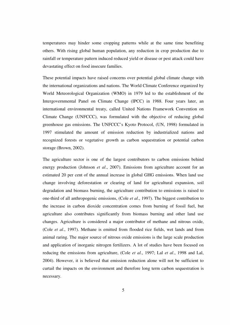
……………………………………………………….…………………….5
Where DBH is the orange tree diameter at 30 cm above the ground
For forked orange trees that have two or three branches emerging below the 30 cm mark,
the DBHi of each branch was measured separately and then the equivalent combined
diameter and calculated as in the equation below.
…………………………………………….……..6
Where DBH1, DBH2, DBH3 are diameters of forked branches
The total aboveground biomass (AGBPlot kg) per plot was calculated by summing the
aboveground biomass per tree (AGBTree kg) of all the trees in the plot as shown below.
……………………………………………………….………….7
The total aboveground biomass (AGBha kg/ha) per hectare was calculated from the
following relationship;
……………………………………………………8
Estimation of the Belowground Biomass
The belowground biomass (BGBha, Mg/ha) was estimated from the ratio of the shoot to
root ratio of 4:1 (Hairah et al., 2010). From this relationship, the BGBha can be
calculated as follows;

22
………………………………………………………………………..…9
The results obtained from this equation can be compared with the BGBha calculated
using the regression equation for the belowground biomass for tropical trees, as shown
below (Timothy et al, 2005);
……………………………………..10
Where BGBha is the belowground biomass density, and AGBha is the aboveground
biomass density (Mg/ha)
Estimation of the total biomass
The total biomass (Biomassha, Mg/ha) was obtained by adding the aboveground and
belowground biomasses.
……………………………………………………….11
To estimate the amount of carbon content (Mg C ha-1
) from biomass, the following
relationship was used:
…………………………………………………………………………12
The Carbon estimated to be sequestered per hectare was then converted to carbon
dioxide equivalents (CO2e.) as follows; the carbon equivalent per plot calculated as the
average of the four allometric equations (equations 1, 2, 3 and 4).
………………………………………………………………….…...….13

23
3.2.2 LCA BASED CARBON FOOTPRINTS OF ORCHARDS
The initial activity in establishing an orchard involves preparing land for planting tree
seedlings. Land is plowed to loosen the soil to facilitate root growth, remove weeds and
form beds or basins that helps tending operations and irrigation. Irrigation and drainage
systems are also created at this time. After planting several activities follow that include
mechanical or chemical weeding, pruning and maintenance. Although citrus can live up
to 100 to 250 years, a conservative 40-year life-span for the orchards was assumed. The
GHG emissions from the initial land clearing and preparation activity were amortized at
the rate of two and half percent per hectare per year. It was assumed that four percent of
established orchard of old, less productive (less than 50% of expected production), or
diseased trees were removed per year and the land is reworked in preparation for the re-
planting of new trees on annual basis, (Muraro, 2008a). The existing trees are removed
and the land plowed, harrowed and the beds formed in readiness for replanting of new
trees. The removed trees were assumed to be burnt resulting in the release of GHG
emissions.
Some of the equipment/machinery reported to be used in the above mentioned
operations included tractors of different sizes, plows and harrows. It was however,
difficult to establish the amount of fuel consumption from the information given by the
farmers. Literature from Ministry of Agriculture and Cooperatives Farm Management
guide (MACO/FAO, 2007) and publication by Hinson et al., (2006) were used to
determine the missing information.
The summary of the GHG emissions considered for each of the ten orchards in this study
included the following;
i) Direct emissions due to burning of fossil fuels including emission of air pollutants
such as volatile organic carbon and carbon monoxide,
ii) Burning of replaced trees (four percent of the plant biomass per hectare),
iii) Emissions from electricity production and use for the electricity used in the pumping
of water for irrigation,

24
iv) Upstream emissions from energy used in the production of fuels-diesel,
v) Upstream emissions from energy used in the production, packaging and transportation
of fertilizer and pesticides and
vi) Nitrous oxide emissions due to application of fertilizers and emissions from crop
residue.
The above listed emissions were summarized, converted to their respective global
warming potentials and summed up. All carbons emissions were considered negative
(carbon sources) and carbon sequestration as positive (carbon sinks) in the data analysis.
i) Direct emissions due to burning of fossil fuels
Greenhouse gas emissions from burning of diesel fuel were estimated using the IPCC
emission factors (IPCC, 2006a). At diesel lower heating value (LHV) energy content of
35.8 MJ/litre, the default carbon dioxide (CO2) emission rate for agricultural diesel
operations is 2650 g CO2, for methane (CH4) is 0.149 g and 1.02 grams for N2O per liter of
diesel combusted, (ANL, 2009; NONROAD Model (EPA, 2004; 2005 and Hinson et al.,
2006).
Emissions of air Pollutants
During the operations of agricultural machinery air pollutants such as volatile organic
carbons (HOC), carbon monoxide (CO), nitrogen oxides (NOx), particulate matter (PM),
and sulfur dioxide (SO2) are released to the air due to fuel (diesel, petrol and others)
combustion. This report only considers HOC and CO emissions which eventually
convert to CO2, a major contributor to global warming. And these emissions were
calculated from the formulas and emission factors used in the US Environmental
Protection Agency’s NOROAD model (EPA, 2004). For a diesel internal compression
ignition (CI) engine, the VOC and CO exhaust emission factors were calculated as
follows:

25
…….……………………………………….14
Where; EFadj is the final emission factor adjusted to account for transient operation and
deterioration in grams per horsepower-hour (g/hp-hr), EFSS is the zero-hour, steady state
emission factor (g/hp-hr), TAF is the transient adjustment factor and DF is the
deterioration factor.
To determine DF and EFSS, the model year, age, horse power size and technology of the
engine has to be known.
The emissions of the particulate matter (PM) are dependent on the sulfur content of the
fuel the engine is burning. To calculate PM, equation 14 was adjusted to account for the
differences in sulfur content of the fuel and is written as follows;
……………………………………………15
Where; SPMadj, defined in the equation below, is the adjustment to PM emission factor to
account for variations in fuel sulfur content (g/hp-hr), PM and SO2 being the only diesel
pollutants that are dependent on fuel sulfur content and EFSS, TAF and DF were defined
in equation 16. Particulate matter (PM) emissions were not considered in this study.
………………………16
……………………….17
Where; age factor is the fraction of median life expended is the
and A and b are constants for a given
pollutant/technology type; b ≤ 1.
Calculation of air pollutants
For a diesel internal compression ignition (CI) engine, the volatile organic carbon and
carbon monoxide exhaust emission factors were calculated as shown below. An 80 HP
tractor and assumed to have been manufactured before 1990 with tier 1 technology and

26
taken to be at its median life (half of life span) in 1990 was considered. The results of
the calculations were shown in Table 20 and Table 21.
For diesel engines, b = 1
Activity hours = 475 (EPA, 2010)
Load factor = 0.59 (EPA, 2010)
Expected Engine life = 4667 hours (EPA, 2010)
Cumulative hours = 2375 hours
The emissions factors are calculated using formulas and tables (Tables; A1, A2, A3 and
A4) from EPA report, (EPA, 2004).
DF = 1 + A*(2375*0.59)/4667, A(HC, CO) = 0.047, 0.185
DF(HC, CO) = 1.014, 1.055
EFSS(HC, CO) = 0.5213, 2.3655
TAF(HC, CO) = 1.05, 1.53
EFadjHC = 0.5213*1.05*1.014 = 0.555 g/hp-hr
EFadjCO = 2.3655*1.53*1.055 = 3.818 g/hp-hr
EFadjHC = 7.36 g/litre
EFadjCO = 50.62 g/litre
Emissions of VOC and CO from land maintenance activities
The calculation of the emissions of VOC and CO for land preparation was also done for
land maintenance using emission factors and formulas, (EPA, 2004).

27
ii) Burning Replaced Citrus Tree
The old trees that were removed from the orchards were assumed to be burned. The
amount of the dry matter to be burned depends on the amount of biomass per tree per
hectare. This was determined by the number of trees replaced per hectare. And the
emissions that are released to the atmosphere during tree burning contain a number of
gaseous species many of which may contribute to net greenhouse emissions and air
pollutant levels. The total emissions released depends upon the amount of matter that
was available to be burned, the fraction that is actually burned and the emission factor
for each species, (Muraro, 2008a and Futch et al 2008). The amount of dry matter that
was estimated to be burnt in the fields studied was taken to be four percent of the
amount of biomass per ha. This means that smaller amounts of biomass was burnt for
smaller trees. The emission factors for different species of GHGs were used, (Andreae
and Merlet, 2001 and IPCC, 2006b).
Amortization of emissions
The investment in initial land preparation and the associated carbon emissions was
spread over an assumed life span of the orchard (40 years) at the rate of two and half
percent per annum. The emissions due to tree burning and land maintenance activities
were also treated as being four percent of the total emissions per hectare.
Cultural Activities
The orchard tending activities, although very necessary contribute to carbon emissions.
The main aims of performing cultural operations are to maintain the orchard in a weed-
free environment, to protect the trees and fruit from damaging insects, microbes and
nematodes, and to provide the plants with adequate water and nutrients. Pruning of the
citrus trees is also done to keep limbs (bearing branches) away from the ground, and to
reduce the amount of vegetative growth and to control the shape and height of the tree to
enhance hand harvesting and allow more light into canopy for attractive colour of fruits.
There are slight differences in the management of young trees (within the first five years
of planting) than with mature ones. The management of weeds was reported to have

28
been done through mechanical cultivation, slashing and the application of herbicides.
Although herbicides are said to be effective and easier in weed control, it was noted that
if not properly applied could affect the quality of the fruits. This however, has not
reduced the importance of herbicides as tools available to the citrus farmer in
management of unwanted plants. The weed population needs to be minimized in order to
eliminate plants that could compete with the shallow-rooted citrus trees for both water
and nutrients. In addition, weeds tend to reflect solar energy, which prevents the
underlying soil from heating up during the day.
Carbon Emissions from cultural practices
The emissions from the cultural practices were calculated from the emissions factors
given in the IPCC guidelines, (IPCC, 2006a).
VOC and CO emissions from cultural activities
The emissions of VOC and CO were calculated using emissions and formulas in US
EPA (EPA, 2004). The calculation of these emission factors depend on the tractor model
technology, the annual activity cumulative hours and the load factor and expected engine
life.
iii) Emissions from electricity used in pumping water for irrigation
The orchards numbered as Plot 1, Plot 2, Plot 3, Plot 4 and Plot 5 were irrigated by
pumping water from boreholes using two pumps powered by three phase electricity from
the main Zambia Electricity Supply Cooperation grid supply lines. The two pumps were
Mono Pumps rated 30 horse power and each of them running for adequate time per day
for every 14 days from April to mid November each year. The pumps were used to
pump the water into reservoir. For Plot 10 water was pumped from a shallow well and
irrigation water for plot 6 was pumped from a stream. The energy consumption is
calculated from the equation 18 given below.
29
………………………………………………………………18
Where; Pir is the input power at full rated load in kW, hp is the nameplate horse power,
ηfl is the efficiency at full-rated load (75%).
iv) Energy for the production of liquid fuels
There is energy that is expended in the acquisition of energy. Electric energy was used
to run pumps, while diesel was used to run tractors. The energy used in the production of
electricity and diesel were calculated from the emission factors given by Argonne
National Laboratories’ GREET Model (ANL, 2009).
Emissions from the Production of electricity and Diesel
Energy related emissions, including emissions from the energy used in the production of
fuel and electricity were calculated using the Greenhouse gases Regulated Emissions
and Energy in Transport (GREET Model: 2011) program developed by the US
Environmental Protection Agency (EPA). The program calculates the energy carbon
emissions associated with the production of fuel and its transportation from the oil field
to the Pump (Filling Station) known as Well to Pump (W-T-P) and are given in grams
per mmBtu. The Model can also calculate the carbon emissions associated with the use
of the fuel commonly referred as well to wheals (W-T-W) which is given in grams per
mile. Using the GREET Model: 2011database, (ANL, 2009; EPA, 2010 and GREET
Model, 2011), the emission factors due to the production of fuels and electricity, after
converting the units to grams per mega joules.
Agro-chemical inputs
To maintain healthy and productive citrus plants, nutrients, pesticides water are applied
to the orchard. The fertilizers Calcium Ammonium Nitrate and Ammonium Nitrate were

30
used as a source of nitrogen, while Potassium Sulphate was used to supply potassium.
Several insecticides, fungicides and herbicides were used to control insects, diseases and
weeds respectively. A Sprayer boom was used to apply the pesticides for small low input
orchards.
v) Energy in-puts in fertilizer and pesticide production
The amount of energy consumed in the production of agricultural chemicals (fertilizers and
pesticides) is significant. The upstream energy for the production, packaging and
transportation of fertilizers are taken from Bhat et al. (1994). The upstream energy for the
manufacture, formulation, packaging and transportation of pesticides were also taken from
Bhat et al. (1994), which is the most comprehensive literature found on the upstream energy
for the production of agro-chemical inputs. The GREET model (ANL, 2009) is used to
determine the values of carbon emissions associated with the manufacture and transportation
of fertilizers and pesticides.
Upstream Emissions from production of fertilizers
The source of energy in the production of fertilizer is derived from Natural gas and
electricity, while that for transportation is usually from diesel in the proportions given by
Bhat et al., (1994). The carbon emissions were determined using the GREET Model,
(ANL, 2009; GREET Model: 2011) and thus apportioned accordingly.
vi) Nitrous oxide emissions due to fertilizer application
Direct greenhouse gas emissions are also released as a consequence of using fertilizers.
The rate at which the emission occurs can be determined using the IPCC guidelines
(IPCC, 2006b). In considering only nitrogen fertilizer application, the rate of direct N2O
emissions can be calculated from the following equation;

31
………………………………19
Where; N2Ofert. emissions is the mass of annual nitrous oxide emissions per unit area due to
fertilization [kg/unit area], Nmass applied is the mass of nitrogen fertilizer, as nitrogen,
applied annually per unit area, EFapplied is the emissions factor for added nitrogen, taken
to be 0.01 per IPCC guidelines (IPCC, 2006b) and N2Omw/(2*Naw) is the conversion
factor for nitrogen to nitrous oxide, equal to 44/28.
Carbon dioxide emissions due to urea application
The application of urea fertilizer to orchards as a source of nitrogen produces emissions
of CO2 as well as N2O. Urea CO(NH2)2 in the presence of water, reacts to form
ammonium (NH4+), hydroxyl ion (OH
-), and bicarbonate (HCO3
-). The bicarbonate ion
then reacts further to form CO2 and water. During the manufacturing of urea, CO2 from
the atmosphere is consumed which is released from the urea upon use. From the IPCC
guidelines it was assumed that all of the carbon in the urea is oxidized to CO2 and
released as emissions to air. The CO2 emissions are calculated as shown in the relations
on the conversion of carbon to carbon dioxide;
CO2emissions = Murea*12/28*44/12
Where; CO2emissions is the mass carbon dioxide emission as result of applying urea,
converted from the nitrogen to carbon dioxide and Murea is the mass of urea applied to a
unit area.
Nitrous oxide due to residue from trimmings left on the field
The exact amount of biomass pruned and left on the ground was not determined. Five
percent (5%) of standing biomass is pruned from citrus trees annually
(UNFCCC/NUCC, 2011). The amount of nitrogen in pruned residues is estimated at

32
0.5% of the total biomass, (IPCC, 2006b). Equation 20 below was used to calculate the
nitrous oxide emissions from the crop residues.
…………………………20
Where; N2OCR is the mass of annual nitrous oxide emissions due to pruning residues per
hectare [kg/ha], MCR, N is the mass of the trimmings as calculated from the average of the
allometric equations, FRACTION Residues is the fraction of nitrogen in the pruning
residues, estimated to be 0.005 for a mixture of leaves and twigs, EF N Residues is the
factor for crop residue nitrogen, taken to be 0.01, as per IPCC guidelines, N2Omw/(2*Naw)
is the conversion factor for nitrogen to nitrous oxide, taken to be equal to 44/28.
Nitrous Oxide due to volatilization for the application of urea
In addition to N2O emissions that are released directly from fertilized cropland, indirect
emissions occur either when N volatilized as NH3 or oxides of nitrogen (NOX) and
subsequently deposited either in its gaseous form or as NH4+ and NO3
- onto soil, water,
or plant surfaces or through the process of nitrification and denitrification by which N2O
is formed and released to the atmosphere. Sources of nitrogen that contribute to indirect
emissions of N2O from citrus farming include chemical fertilizer application and crop
residues (tree trimmings left on the ground after pruning), EPA, (2010). The nitrous
oxide indirect emissions are accounted for using IPCC guidelines (IPCC, 2006b), as
shown in the equation 21 (due to volatilization) and equation 22 (due to leaching) below.
………21
Where; N2Ovolatilization is the mass of annual nitrous oxide emissions per unit area
produced from atmospheric deposition of nitrogen volatilized from crop land [kg], N mass
is the mass of nitrogen fertilizer, as nitrogen, applied annually per unit area [kg],
FRACTION volatilization is the fraction of the synthetic fertilizer that volatilizes, assumed to
be 0.1 in accordance to IPCC guidelines (IPCC, 2006b), EFvolatilization is the mass of
annual direct nitrous oxide emission per unit area due to the application of nitrogen

33
fertilizer which is taken to be 0.01 (IPCC, 2006b) and N2Omw/(2*Naw) is the conversion
factor for nitrogen to nitrous oxide, taken to be equal to 44/28.
Nitrous Oxide due to leaching for the application of urea
……………..22
Where; N2Oleach is the mass of annual nitrous oxide emissions per unit area produced
from leaching and runoff of nitrogen from crop land [kg], Nfert is the mass of nitrogen
fertilizer, as nitrogen, applied annually per unit area, Nbiomass is the mass of nitrogen in
biomass remaining on the ground per unit area (0.5% of biomass), FRACTIONleach is the
fraction of added nitrogen that volatilizes, taken to be 0.30 (IPCC, 2006), EFleach is the
mass of annual direct nitrous oxide emission per unit area due to the leaching of
nitrogen; assumed to be 0.0075 as per IPCC guidelines, (IPCC, 2006b) and
N2Omw/(2*Naw) is the conversion factor for nitrogen to nitrous oxide, taken to be equal to
44/28.
Calculation of Nitrous Oxide emissions due to fertilizer application
N2Ofert. emission = 289.5*0.01*44/28 = 4.55 kg/ha
Carbon dioxide emissions due to urea application
CO2emissions = 0*12/28*44/12 = 0 kg/ha
Nitrous oxide due to residue from trimmings left on the field
N2OCR = 1550.33*0.005*0.01*44/28 = 0.122 kg/ha
Nitrous Oxide due to volatilization for the application of urea
= 289.5*0.1*0.01*44/28 = 0.455 kg/ha
Nitrous Oxide due to leaching for the application of urea
= (289.5+7.75)*0.3*0.0075*44/28 = 1.051 kg/ha
34
Energy Requirements for the production of pesticides
As noted from section 3 above, the upstream energy in the production of pesticides was
taken from Bhat et al., (1994). The unit energy consumed in producing active
ingredients of herbicides, insecticides and fungicides are calculated as 214.93, 245.06
and 356.39 MJ/kg respectively. The active ingredients (a.i.) are formulated into usable
forms before being released into the market. The forms into which pesticides are
formulated into include emulsifiable oils, wettable powders and granules. Green (1987)
estimated that formulation into emulsifiable oil, wettable powder and granules requires
an additional energy of 20, 30 and 10 MJ/kg, respectively. In addition the energy
required for packaging and distribution of pesticides was estimated to be about 2 MJ/kg.
The energy used for transportation depends on the distance pesticides are distributed. If
the pesticides are domestically produced and used, distribution energy is estimated to 1
MJ/kg. The energy used in the distribution is 5 MJ/kg for pesticides imported from other
countries, (Bhat et al., 1994).
Green house gas emissions from the production of pesticides
The emission factors were calculated using the GREET Model: 2011. The actual
emissions were then calculated by multiplying the emission factors of particular energy
source in grams per Mega Joule by the amount of upstream energy, (ANL, 2009) (The
GREET Model: 2011).
Converting LCA results to Carbon equivalents
For purposes of determining the net carbon sequestration potential of orchards, each of
the greenhouse gases was converted to its carbon dioxide equivalents using their
respective 100 year global warming potentials (PAS 2050, 2011). These factored
emissions were then summed up to give the total emissions in terms of carbon dioxide
equivalents. Volatile organic carbon gases and carbon monoxide are assumed to be
readily oxidized to carbon dioxide and volatile organic carbon gases have a relatively
low molecular weight consisting of 83 wt% carbon, (EPA, 2010). Therefore, the sum of

35
the masses of greenhouse gas emissions as expressed in terms of carbon equivalents are
given as shown in the equation 23 below:
………23
Where; GHGTotal Carbon Equivalents is the sum of the greenhouse gas emissions expressed as
carbon dioxide equivalents, mi is the mass of emissions of greenhouse gas species i (e.g.
CO2, CH4 or N2O), GWPi is the 100 year global warming potential for greenhouse gas i,
mCO is the mass of carbon monoxide emissions, CO2mw/COmw is the conversion factor for
CO to CO2, taken to be equal to 44/28, mVOC is the mass of VOC emissions and
CO2mw/Caw is the conversion factor for C to CO2, calculated to be equal to 44/12.

36
Chapter 4
4.0 RESULTS
4.1 BIOMASS DETERMINATION: HIGH-INPUT ORCHARD SYSTEMS
4.1.1 Biomass Determination (Carbon sequestration) for Plot 1 in Kafue district
A 30 m by 60 m (1800 m2) sampling area was marked out in the middle of a commercial
orchard. It consisted of a total of fifty one (51) 35-year-old citrus trees of the variety
Washington Navel (Citrus sinensis) on Lemon rootstock (Citrus jambari). All the 51
trees had their diameter at 30 cm aboveground (DBH) measured and recorded in
booking forms. Four trees in the plot were dead and required replacement while a few
others showed stress effects of poor growth and were reported to be low yielding. The
dead trees were left out in the analysis while the stressed low yielding trees were
included in the analysis for biomass.
The slope of the field was generally flat (0.1º) and the orchard was generally well
maintained and was therefore weed free (Figure 4). The summary of the results of the
calculation of biomass is shown in Table 3. Using equations 1-12, the average carbon
stock was found to be 19.4 Mg C/ha. Equation 13 was used to convert the carbon stock
into carbon dioxide equivalents.

37
Figure 4: Picture of a high-input citrus orchard (Plot 1) in Kafue district
Table 3: Carbon stock and sequestration results for citrus trees in Plot 1 determined
using four different allometric equations
Equation Eq. 1 Eq. 2 Eq. 3 Eq. 4 Average
Plot Aboveground Biomass per
equation (kg/Plot Area)
6253.25 4370.81 5221.27 6479.43 5581.19
Expansion Factor 5.56 5.56 5.56 5.56 5.56
Aboveground Biomass (kg/ha) 34740.29 24282.30 29007.03 35996.81 31006.61
Belowground Biomass (kg/ha) 8685.07 6070.57 7251.76 8999.20 7751.65
Total Biomass (kg/ha) 43425.37 30352.87 36258.79 44996.01 38758.26
Carbon (kg C/ha) 21712.68 15176.44 18129.40 22498.01 19379.13
Carbon Equivalents (kg CO2e/ha) 79620.41 55651.99 66480.49 82500.19 71063.27
A regression analysis was done to determine the correlation between DBH and the tree
average biomass (kg/tree). The regression coefficient was found to be 0.974 and was
highly significant (Table 15).

38
4.1.2 Biomass (Carbon sequestration) of citrus trees in Plot 2 in Kafue district
This plot had 50 trees and was 1800 m2 in size and was generally flat like most of
agriculture fields. There were four dead citrus trees which were not included in the
biomass determination. This farm can be considered a high input system although with a
lower level of management compared to Plot 1. More trees had been replaced due to the
drying of old ones. The results of the calculations are shown in Table 4 and the carbon
stock calculated from equations 1 to 12 is given as 21.2 Mg C/ha.
Table 4: Plot 2 carbon stock and sequestration results
Equation Eq. 1 Eq. 2 Eq. 3 Eq. 4 Average
Plot Aboveground Biomass per
equation (kg/Plot Area)
6943.14 4872.10 5627.07 7011.06 6113.34
Expansion Factor 5.56 5.56 5.56 5.56 5.56
Aboveground Biomass (kg/ha) 38572.99 27067.21 31261.50 38950.33 33963.01
Belowground Biomass (kg/ha) 9643.25 6766.80 7815.37 9737.58 8490.75
Total Biomass (kg/ha) 48216.24 33834.02 39076.87 48687.92 42453.76
Carbon (kg C/ha) 24108.12 16917.01 19538.44 24343.96 21226.88
Carbon Equivalents (kg CO2e/ha) 88404.48 62034.67 71647.44 89269.29 77838.97
The increase DBH resulted in increase in biomass per tree. Trees with higher DBH
diameters produced high biomass. This was confirmed by regression analysis which
gave the regression coefficient of 0.984. Regression coefficients of the results from each
equation (equations 1, 2, 3 and 4) were calculated (Table 15).
4.1.3 Biomass (Carbon sequestration) results in Plot 3 in Kafue district
This plot was set out to be 30 m by 66 m, giving a plot size of 1980 m2. It had 55 citrus
trees. The slope of the plot was measured to be zero degrees. The plot was free from
weeds at the time of the study. Two citrus trees were dead in the plot and therefore, not
taken as part of the measured trees. There were several trees with forked branches which
necessitated the calculation of equivalent DBHs as shown in equation 6. The huge

39
number of forked branches is an indication that proper thinning of the citrus trees in their
young age was not religiously followed. The DBH of each and every tree was measured
and recorded in booking forms. Some of the tree heights were measured and generally
averaged 6 meters. The results of biomass calculations were as summarized in Table 5.
The carbon stock was calculated as 23.3 Mg C/ha which is given as 85.5 Mg CO2e/ha.
Table 5: Carbon stock and sequestration Results for Plot 3 in Kafue district
Equation Eq. 1 Eq. 2 Eq. 3 Eq. 4 Average
Plot Aboveground Biomass per
equation (kg/Plot Area)
8301.99 6041.29 6743.67 8453.75 7385.17
Expansion Factor 5.05 5.05 5.05 5.05 5.05
Aboveground Biomass (kg/ha) 41929.25 30511.54 34058.92 42695.73 37298.86
Belowground Biomass (kg/ha) 10482.31 7627.89 8514.73 10673.93 9324.71
Total Biomass (kg/ha) 52411.56 38139.43 42573.65 53369.66 46623.57
Carbon (kg C/ha) 26205.78 19069.71 21286.83 26684.83 23311.79
Carbon Equivalents (kg CO2e/ha) 96096.59 69928.64 78058.80 97853.27 85484.32
Lower coefficient of correlation was calculated for the relationship between DBH and
tree biomass. The coefficient of correlation (r2 = 0.883) was still higher than 0.5 which
shows that the increase biomass can be explained in terms of the increase in DBH,
(Table 15).
4.1.4 Biomass (Carbon sequestration) of Plot 4 in Kafue district
This plot is part of a commercial or high input orchard. This plot had 48 plants in an
orchard with a plant population of 277. The plant spacing was 6 m by 6 m. The plant
height was generally above 6.4 m. There was one tree missing. The orchard was weed
free and the trees looked health and free of stress and disease. The highest DBH
recorded for this plot was 25.1 cm. This necessitated the use of allometric equations
which had higher range of allowable diameters (DBHs). The average biomass was
calculated and the results were as given in Table 6.

40
Figure 5: Picture of a commercial (high-input) orchard (Plot 4) in Kafue district
Table 6: Biomass (carbon sequestration) results for Plot 4 in Kafue district
Equation Eq. 1 Eq. 2 Eq. 3 Eq. 4 Average
Plot Aboveground Biomass per
equation (kg/Plot Area)
7574.72 5336.60 6093.89 7603.03 6652.06
Expansion Factor 5.56 5.56 5.56 5.56 5.56
Aboveground Biomass (kg/ha) 42115.42 29671.50 33882.05 42272.86 36985.46
Belowground Biomass (kg/ha) 10528.86 7417.88 8470.51 10568.22 9246.36
Total Biomass (kg/ha) 52644.28 37089.38 42352.56 52841.08 46231.82
Carbon (kg C/ha) 26322.14 18544.69 21176.28 26420.54 23115.91
Carbon Equivalents (kg CO2e/ha) 96523.28 68003.38 77653.41 96884.12 84766.05
The regression coefficient was very close to one (0.989), and the regression analysis was
as shown in Table 15.

41
4.1.5 Biomass (Carbon sequestration) of Plot 5 in Kafue district
The sample plot size was 36 m by 60 m (2160 m2) and the resulting expansion factor
being 4.63 was used. The calculated carbon stock for this plot is shown in Table 7. Plot
5 was located in the center part of the high input commercial orchard of about 2 ha. The
field slope was measured as zero degrees. The orchard was weed free, stress and disease
free. Plant spacing like the other plots was 6 m by 6 m. There were 59 trees in the plot,
but had a high number six (6) trees were either dead or had dried up and had not been
replaced.
Table 7: Carbon stock and sequestration results for plot 5
Equation Eq. 1 Eq. 2 Eq. 3 Eq. 4 Average
Plot Aboveground Biomass per
equation (kg/Plot Area)
8366.57 5981.80 6739.73 8421.00 7377.28
Expansion Factor 4.63 4.63 4.63 4.63 4.63
Aboveground Biomass (kg/ha) 38737.23 27695.74 31204.95 38989.23 34156.79
Belowground Biomass (kg/ha) 9684.31 6923.93 7801.24 9747.31 8539.20
Total Biomass (kg/ha) 48421.53 34619.67 39006.19 48736.54 42695.98
Carbon (kg C/ha) 24210.77 17309.84 19503.09 24368.27 21347.99
Carbon Equivalents (kg CO2e/ha) 88780.88 63475.17 71517.84 89358.44 78283.08
The regression analysis relating the DBH and tree biomass was performed to confirm the
correlation and regression coefficient was found to be 0.854. The summary of the
analysis is shown in Table 15.
Summary of carbon sequestration for high input plots
Table 8 shows a summary of carbon sequestration for the high-input orchards. The
carbon stock per ha was found to be 21.66 Mg C/ha and the carbon dioxide equivalents
was 79.5 Mg CO2e/ha with an annual carbon dioxide equivalents increment of 7.62 Mg
CO2e/ha per year.

42
Table 8: Summary of carbon stock and sequestration results for the five high input
orchards
Orchard Biomass
(Mg/ha)
Carbon Stock
(Mg C/ha)
Carbon Eq. (Mg
CO2e/ha)
Annual CO2e Increment
(Mg CO2e/ha)
Plot 1 38.8 19.4 71.1 7.28
Plot 2 42.5 21.2 77.8 7.54
Plot 3 46.6 23.3 85.5 7.87
Plot 4 46.2 23.1 84.8 8.04
Plot 5 42.7 21.3 78.3 7.32
Average 43.36 21.66 79.5 7.61
4.2 LOW-INPUT CITRUS ORCHARDS
4.2.1 Biomass (Carbon sequestration) of Plot 6 in Lusaka district
The trees in this plot were planted in 1984 and as was the case with the other orchards
they comprised of Washington Navel (Citrus sinensis) variety grafted on the Lemon
(Citrus jambari) rootstock. The seedlings were reported to have been sourced from
University of Zambia nursery in Chilanga. Total enumeration was used on this plot
which measured 24 m by 65 m (1560 m2). There were 73 plants in this plot which
translated to a slightly higher plant density of 450 plants per hectare. The tree size
generally looked smaller than they should, considering their age. At the time of the
study, the field was not weed free; the orchard was infested with Nidorella resedifolia
and grass weeds such as Eleusine indica. There seemed not much of pruning and
thinning done. Some lemon branches had grown from the rootstock and become trees at
full bearing age and in fact, lemons were reported to be a favoured source of revenue
from the sales of lemon fruits as compared to orange fruits.

43
Figure 6: Picture showing small holder orchard (Plot 6) in Lusaka district
The results of the biomass determination are shown in Table 9. The carbon stock was
17.6 Mg C/ha.
Table 9: Carbon stock and sequestration results for Plot 6 in Lusaka district
Equation Eq. 1 Eq. 2 Eq. 3 Eq. 4 Average
Plot Aboveground Biomass per
equation (kg/Plot Area)
4643.17 3199.96 4399.86 5345.76 4397.19
Expansion Factor 6.41 6.41 6.41 6.41 6.41
Aboveground Biomass (kg/ha) 29762.72 20511.73 28203.08 34266.32 28185.96
Belowground Biomass (kg/ha) 7440.68 5127.93 7050.77 8566.58 7046.49
Total Biomass (kg/ha) 37203.40 25639.66 35253.84 42832.90 35232.45
Carbon (kg C/ha) 18601.70 12819.83 17626.92 21416.45 17616.23
Carbon Equivalents (kg CO2e/ha) 68212.43 47010.32 64637.92 78534.13 64598.70
The regression coefficient was 0.988 and the rest of the parameters were shown in Table
15.

44
4.2.2 Biomass (Carbon sequestration) of Plot 7 in Kafue district
Plot 7 was a small orchard belonging to a small holder farmer located on fertile flat plain
with a chance of flooding in times of heavy rains as reported by the farmers. It was
planted in 1992. Standard plant spacing of 5 m by 5 m was used. Two varieties of
oranges were noticed and these were Hamlin and Washington Navel which were sourced
from Mungu Nursery in Kafue district. The orchard was weed free and clean (Figure 7).
There were 25 plants, three of which had deteriorated to the level where they needed
replacement. Total enumeration was done in this plot which measured 625 m2; all the
trees had their DBH measured. The slope of the land was zero degrees and expansion
factor was 16. The carbon stock (25.5 Mg C/ha) in this plot is higher than that calculated
for high input orchards. The rest of the results were shown in Table 10.

45
Figure 7: Picture showing low-input orchard (Plot 7) in Chikupi area of Kafue district
Table 10: Plot 7 carbon stock and sequestration results
Equation Eq. 1 Eq. 2 Eq. 3 Eq. 4 Average
Plot Aboveground Biomass per
equation (kg/Plot Area)
2860.20 1916.22 2433.96 3002.06 2553.11
Expansion Factor 16.00 16.00 16.00 16.00 16.00
Aboveground Biomass (kg/ha) 45763.20 30659.57 38943.40 48033.01 40849.78
Belowground Biomass (kg/ha) 11440.80 7664.89 9735.85 12008.25 10212.45
Total Biomass (kg/ha) 57204.00 38324.46 48679.25 60041.27 51062.23
Carbon (kg C/ha) 28602.00 19162.23 24339.62 30020.63 25531.11
Carbon Equivalents (kg CO2e/ha) 104874.95 70262.14 89246.10 110076.66 93614.93
The regression coefficient was 0.995, an indication that the increase in biomass was as a
result of the increase in DBH. Table 15 shows the rest of the parameters determined
from regression analysis.

46
4.2.3 Biomass (Carbon sequestration) of Plot 8 in Kafue district
Plot 8 was marked out from an orchard that was planted in 1974 and is among the oldest
of the fields studied. It is located in a fertile flat plain, about 6 km from plot 7. It
belonged to a small holder farmer. Nitrogenous fertilizer was reported by the owner to
have been applied for a period from 1976 to 1980. The varieties planted included the
Washington Navel and Valencia. The orchard was 0.25 ha and a 600 m2 plot was
marked out from the middle of the orchard. The plot had 15 trees (Figure 8). The water
for irrigation was drawn from shallow wells located within the orchard. The plot was
flat, field slope being zero degrees and expansion factor was 16.67. The carbon stock
was 29.8 Mg C/ha as shown in Table 11.

47
Figure 8: Picture showing citrus trees in a Low input orchard (Plot 8) in Kafue district
Table 11: Carbon stock and sequestration results for Plot 8 in Chikupi area of Kafue
district
Equation Eq. 1 Eq. 2 Eq. 3 Eq. 4 Average
Plot Aboveground Biomass per
equation (kg/Plot Area)
3208.56 2460.15 2549.72 3221.82 2860.06
Expansion Factor 16.67 16.67 16.67 16.67 16.67
Aboveground Biomass (kg/ha) 53475.96 41002.49 42495.39 53697.03 47667.72
Belowground Biomass (kg/ha) 13368.99 10250.62 10623.85 13424.26 11916.93
Total Biomass (kg/ha) 66844.95 51253.11 53119.23 67121.29 59584.65
Carbon (kg C/ha) 33422.47 25626.56 26559.62 33560.65 29792.32
Carbon Equivalents (kg CO2e/ha) 122550.19 93964.89 97386.15 123056.82 109239.51
The regression coefficient for DBH and tree biomass was 0.978 at a probability of less
than 0.001 (Table 15).

48
4.2.4 Biomass (Carbon sequestration) of Plot 9 in Palabana area of Chongwe
district
Plot 9 planted in 2005 represented the youngest plants of the study, (six years). The
orchard was slightly less than 0.25 ha in size, comprising of two parts; one planted with
oranges (Citrus sinensis) and the other planted with tangerines (C. reticulata) and
peaches (Prunus persica). The focus of this study was on the side planted with oranges
which measured 900 m2 and a total enumeration was done. All the 43 plants in the plot
had their DBH measured, (Figure 9). The tree heights were generally around 3 m and the
average DBH was 9.49 cm. The Carbon Stock was calculated to be 7.2 Mg C/ha. From
this single field, one can safely conclude that biomass accumulation was influenced by
age, although it was not the only factor. The rest of the results are shown in Table 12.
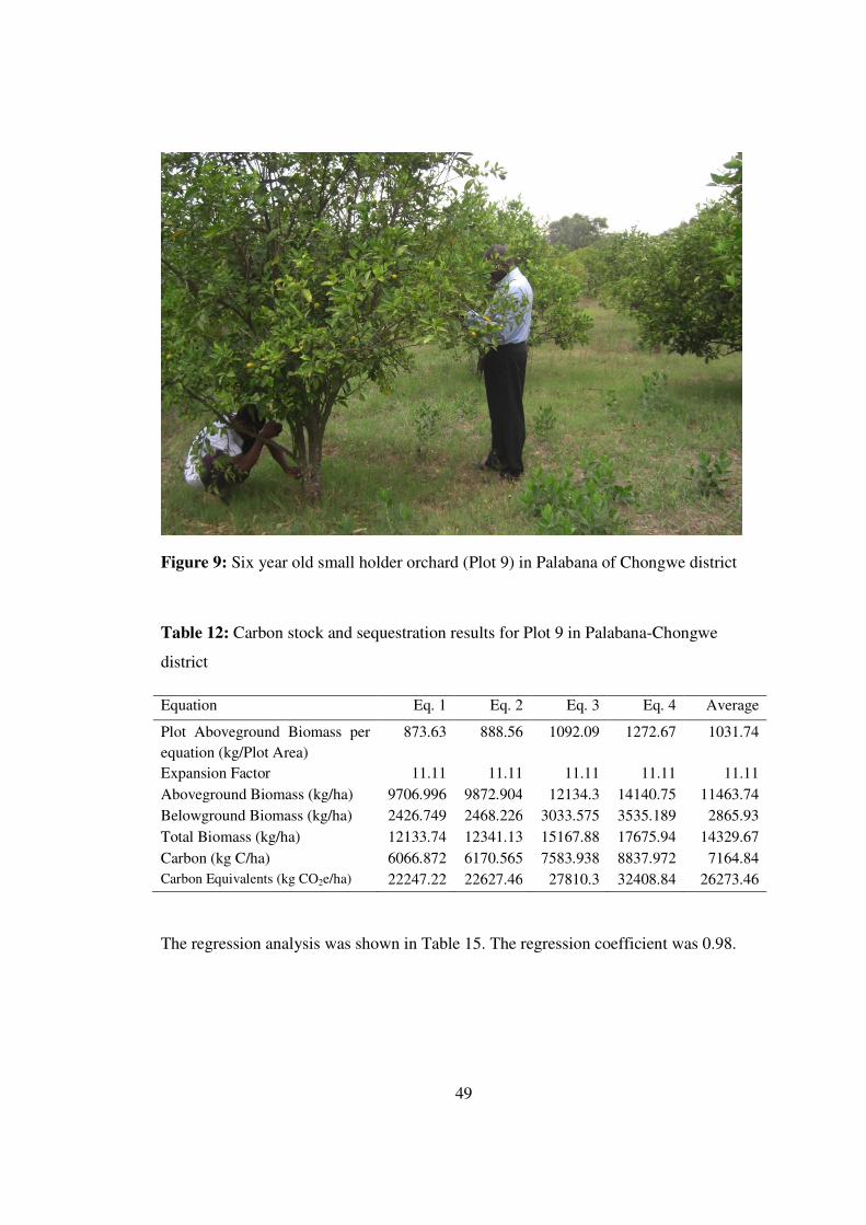
49
Figure 9: Six year old small holder orchard (Plot 9) in Palabana of Chongwe district
Table 12: Carbon stock and sequestration results for Plot 9 in Palabana-Chongwe
district
Equation Eq. 1 Eq. 2 Eq. 3 Eq. 4 Average
Plot Aboveground Biomass per
equation (kg/Plot Area)
873.63 888.56 1092.09 1272.67 1031.74
Expansion Factor 11.11 11.11 11.11 11.11 11.11
Aboveground Biomass (kg/ha) 9706.996 9872.904 12134.3 14140.75 11463.74
Belowground Biomass (kg/ha) 2426.749 2468.226 3033.575 3535.189 2865.93
Total Biomass (kg/ha) 12133.74 12341.13 15167.88 17675.94 14329.67
Carbon (kg C/ha) 6066.872 6170.565 7583.938 8837.972 7164.84
Carbon Equivalents (kg CO2e/ha) 22247.22 22627.46 27810.3 32408.84 26273.46
The regression analysis was shown in Table 15. The regression coefficient was 0.98.

50
4.2.5 Biomass (Carbon sequestration) of Plot 10 of Chikupi area of Kafue district
Plot 10 Orchard was planted in 1991. The citrus tree varieties were Washington Navel
and Hamlin grafted on rough lemon (Citrus limon) which were sourced from Mungu
Nursery of Kabweza area of Kafue district. The orchard was 1100 square meters and
total enumeration was employed and all the 42 trees had their DBH measured. The plot
was flat and the expansion factor was determined to be 9.09. The field was weed and
disease free and the trees looked health and big. Like Plot 7 and Plot 8, Plot 10 was
located in a fertile plain. The carbon stock was determined to be 22.3 Mg C/ha as shown
with the rest of the results in Table 13.
Figure 10: Picture of Low input orchard (Plot 10) in Kafue district

51
Table 13: Carbon stock and sequestration results for Plot 10 in Kafue district
Equation Eq. 1 Eq. 2 Eq. 3 Eq. 4 Average
Plot Aboveground Biomass per
equation (kg/Plot Area)
4420.71 2851.46 3787.85 4650.60 3927.65
Expansion Factor 9.09 9.09 9.09 9.09 9.09
Aboveground Biomass (kg/ha) 40184.22 25919.77 34431.56 42273.96 35702.38
Belowground Biomass (kg/ha) 10046.06 6479.94 8607.89 10568.49 8925.59
Total Biomass (kg/ha) 5030.28 32399.71 43039.46 52842.44 44627.97
Carbon (kg C/ha) 25115.14 16199.86 21519.73 26421.22 22313.99
Carbon Equivalents (kg CO2e/ha) 92097.21 59404.88 78912.84 96886.62 81825.39
The regression coefficient was 0.993 as shown Table 15.
4.3 Summary of carbon sequestration for the low input plots
The average carbon sequestration for the low input was 23.8 Mg C/ha, 87.3 Mg CO2e/ha
and 9.35 Mg CO2e/ha for carbon stock, carbon dioxide equivalents and annual CO2e
increment per hectare respectively, as shown in Table 14. When averaging carbon
sequestration, only four plots whose trees were older than 19 years were considered
leaving out Plot 9 representing young six year old trees
Table 14: Average carbon sequestration results for four low input orchards
Orchard Biomass
(Mg/ha)
Carbon Stock
(Mg C/ha)
Carbon Eq. (Mg
CO2e/ha)
Annual CO2e Increment
(Mg CO2e/ha)
Plot 6 35.2 17.6 64.6 8.67
Plot 7 51.1 25.5 93.6 10.29
Plot 8 59.6 29.8 109.2 9.01
Plot 10 44.6 22.3 81.8 9.43
Average 47.63 23.80 87.30 9.35

52
4.3.1 Regression Analysis
The regression analysis of the ten orchards to determine the correlation between DBH
and tree biomass accumulation (kg/tree) was done and summarized in Table 15.
Table 15: Summary of regression analysis results for DBH against biomass
accumulation
Plot R2 f Significance f t-test p-value Equation
Plot 1 0.9731 1630 0.000 -22.884 0.000 Y = 14.331X - 159.15
Plot 2 0.984 1697 0.000 -28.893 0.000 Y = 14.88X – 170.32
Plot 3 0.883 385 0.000 -10.07 0.000 Y = 14.74X – 157.65
Plot 4 0.989 4192 0.000 -38.5 0.000 Y = 16.66X – 209.52
Plot 5 0.985 3115 0.000 -30.03 0.000 Y = 14.92X – 171.06
Plot 6 0.927 878 0.000 -17.44 0.000 Y = 10.73X – 95.27
Plot 7 0.996 5095 0.000 -44.89 0.000 Y = 15.14X – 176.81
Plot 8 0.978 576 0.000 -11.91 0.000 Y = 16.14X – 191.01
Plot 9 0.980 1970 0.000 -20.41 0.000 Y = 4.47X – 20.41
Plot 10 0.993 5296 0.000 -43.8 0.000 Y = 13.17X – 142.34
4.3.2 Biomass Analysis
The biomass accumulation per plot were summarized in Table 16 and Figure 11 below
which also shows the biomass converted to carbon dioxide equivalents in mega grams
carbon dioxide equivalent per hectare.
Table 16: Summary carbon sequestration results from ten orchards
Orchard Biomass
(Mg/ha)
Carbon Stock
(Mg C/ha)
Carbon Eq. (Mg
CO2e/ha)
Annual CO2e Increment
(Mg CO2e/ha)
Plot 1 38.8 19.4 71.1 7.29
Plot 2 42.5 21.2 77.8 7.54
Plot 3 46.6 23.3 85.5 7.87
Plot 4 46.2 23.1 84.8 8.04
Plot 5 42.7 21.3 78.3 7.32
Plot 6 35.2 17.6 64.6 8.67
Plot 7 51.1 25.5 93.6 10.29
Plot 8 59.6 29.8 109.2 9.00
Plot 9 14.3 7.2 26.3 5.34
Plot 10 44.6 22.3 81.8 9.44

53
Figure 11: Biomass and carbon sequestration, with annual CO2e increment in citrus
orchards
DETERMINATION OF CARBON EMISSIONS FROM FIVE LOW INPUT
ORCHARDS-LCA BASED CARBON FOOTPRINTS OF ORCHARDS
4.4 HIGH INPUT ORCHARDS
4.4.1 Emission for High input Plots
The high input orchards included plots numbered as 1, 2, 3, 4 and 5 and had similar
reported inputs, although the calculated emissions for each individual plot were
different. The exact planting date for the citrus trees were unknown by the farm manager
in-charge of the farm at the time of the study. They were said to have been planted over
30 years before. These Plots were parts of commercial orchards with high levels of
inputs having been applied for a continuous period of 15 years leading to the citrus peak
bearing age. The agro-chemicals used are given in Table 31. In addition to agro-

54
chemicals, consideration was given to other unit operations involved in the growing of
citrus such as land preparation and management, application of fertilizer and pesticides,
irrigation and trimmings, recorded as in booking forms. Other operations such as
planting seedlings and harvesting were not considered as they were generally done
manually and therefore, were carbon neutral or had an insignificant carbon footprint.
Transportation of the fruits was taken to be outside the system boundary.
The initial activity in establishing an orchard was to prepare the land for planting tree
seedlings. Land was plowed to loosen the soil to facilitate root growth and bed formation
to facilitate tending and harvesting operations. Irrigation and drainage systems were also
created at this time. There was a concrete water reservoir into which water was pumped
for storage before being released into the orchards by gravity using concrete lined canals
(now disused) and Poly vinyl chloride (PVC) pipes. Although citrus can live up to 100
years, a conservative 40-year life-span for the orchards was assumed. Four percent of
established orchard of old, non-productive, or diseased trees were assumed to be
removed per year and the land was reworked in preparation for the planting of new trees
on annual basis, (Muraro, 2008a). The existing trees were removed and the land plowed,
harrowed and the beds formed in readiness for replanting of new trees.
All carbons emissions were considered negative (carbon sources) and carbon
sequestration as positive (carbon sinks).
Table 17 shows the equipment and machinery that were used in land preparation for the
establishment of an orchard. Since this farm was established many decades before the
study was conducted and that the management of the farm has changed hands, it was
difficult to determine the exact equipment and fuel consumption at the time of
establishment. An 80 horse power (HP) tractor which was found at the farm was
considered in the calculations. At establishment, the farmers plow and harrow land. The
duration of the operations and fuel consumptions are shown in Table 18, and Table 19
shows the GHG emissions from the burning of fossil fuel in the running of the tractor for
initial land preparations.

55
Table 17: Initial land preparation equipment and fuel consumption per ha
Equipments Size of
tractor
(HP)
Tractor Fuel
consumption
Tractor
Performance
Frequency of
operation per
year
Total fuel
consumption
Litre/ha hr/ha (litre/ha)
Plow 80 12 4 1 48
Row Disk 80 7 2 2 28
Blade 80 12 4 1 48
Total 124
Table 18: Land maintenance equipment and fuel consumption per ha. Land maintenance
was performed after old or unproductive trees were removed in readiness to plant new
ones.
Equipments Size of
tractor
(HP)
Tractor Fuel
consumption
Tractor
Performance
Frequency
of operation
per year
Total fuel
consumption
Litre/ha hr/ha (litre/ha)
Row Disk 80 7 2 2 28
Sub-Soillers 80 7 2 1 14
Total 42
Table 19: Direct GHG emissions from burning of fossil fuel in the operation of tractor
for initial land preparations
Activity Fuel used Emissions factors (g/litre) Emissions (g/ha)
l/ha CO2 CH4 N2O CO2 CH4 N2O
Land Preparation 124 2650 0.149 1.02 326,600 18.48 126.48
Land maintenance 42 2650 0.149 1.02 111,300 6.26 42.84
Sub-Total 166

56
Table 20: Volatile organic carbon and carbon monoxide emissions from tractor exhaust
during initial land preparation activities
Activity Tractor
Power
Fuel consumption
rate
Emissions factors
(g/litre)
Emissions (g/ha)
(HP) (liter/ha) VOC CO VOC CO
Plowing 80 48 7.36 50.62 353.28 2429.76
Row Disking 80 28 3.68 25.31 103.04 708.68
Blade 80 48 7.36 50.62 353.28 2429.76
Sub-Total 809.6 5568.2
Table 21: Volatile organic carbon and carbon monoxide exhaust emissions from tractor
during land maintenance activities in preparation for tree replacement
Activity Tractor
Power
Fuel consumption
rate
Emissions factors
(g/litre)
Emissions (g/ha)
(HP) (liter/ha) VOC CO VOC CO
Row Disking 80 28 3.68 25.31 103.04 708.68
Sub-soiler 80 14 7.36 50.62 103.04 708.68
Sub-Total 206.08 1,417.36
Table 22: Emission factors due to burning of dry matter of citrus trees removed due to
old age and low productivity. Four percent of biomass per ha is replaced annually.
Emissions
factor
Equation 1
(kg/ha)
Equation 2
(kg/ha)
Equation 3
(kg/ha)
Equation 4
(kg/ha)
Average
(kg/ha)
Biomass (g/kg dry
matter
burned)
1737.01 1214.11 1450.35 1799.84 1550.33
GHG
Emissions (g/ha)
CO2 1569 2725376.0 1904946.3 2275601.7 2823949.6 2432468.4
CH4 4.7 8164.0 5706.3 6816.7 8459.3 7286.6
N2O 0.26 451.6 315.7 377.1 468.0 403.1
VOC 5.7 9901.0 6920.5 8267.0 10259.1 8836.9
CO 107 185860.6 129910.3 155187.6 192582.9 165885.4

57
Table 23: Spreading of GHG emissions from initial land preparations at two and half
percent per annum and emissions from the burning of biomass and land maintenance
were amortized at the rate of four percent per annum.
Activity Amortized emissions
over 40 years
Unit
Diesel Land
preparation
Land
Maintenance
Burning
Volume 124 42 4.16 l/ha
Energy 4,439.2 1,503.6 148.93 MJ/ha
VOC 809.6 206.08 8836.9 381.96 g/ha
CO 5,568.2 1,417.36 165885.4 6831.32 g/ha
Greenhouses Gases
CO2 326,600 111,300 0 12617 g/ha
CH4 18.48 6.26 7286.6 292.18 g/ha
N2O 126.48 42.84 403.1 21.000 g/ha
Table 24: Equipment used in orchards for cultural practices of mowing, spraying and
mechanical fertilizer application and their respective fuel consumption in the
management of citrus orchards used in the study.
Activity Size of
tractor
(HP)
Tractor Fuel
consumption
Tractor
Performance
Frequency of
operation per
year
Total fuel
consumption
Litre/ha hr/ha (litre/ha)
Rotary Mower 80 7 2 4 56
Sprayer Boom 80 7 2 6 84
Fertilizer Spread 80 7 2 4 56
Total 196

58
Table 25: Emissions from fuels used in orchard management practices
Fuel Energy
consumption
(litre/ha)
Emissions factor (g/litre) Emissions (g/ha)
CO2 CH4 N2O CO2 CH4 N2O
Diesel 196 2650 0.149 1.02 519,400 29.20 199.92
Sub-Total 519,400 29.20 199.92
Table 26: Volatile organic carbon and carbon monoxide exhaust emissions from tractor
used in tending activities of spraying, fertilizer application and mowing of weeds.
Activity Tractor
Power
Fuel
consumption rate
Emissions factors
(g/litre)
Emissions (g/ha)
HP) (liter/ha) VOC CO VOC CO
Rotary Mower 80 56 1.84 12.655 103.04 708.68
Sprayer Boom 80 84 1.23 8.437 103.32 708.71
Fertilizer Spread 80 56 1.84 12.655 103.04 708.68
Sub-Total 309.4 2,126.07
Table 27: Energy consumption from pumping water for irrigation was calculated from
equation 18. Water was pumped into a reservoir from which it was made to flow by
gravity to individual citrus trees.
Pump Type Nameplate HP KW MJ/ha
Mono Pump 30 29.83 477.28
Mono Pump 30 29.83 477.28
Submersible Pump 7.5 7.46 477.44
Total 1432

59
Table 28: Upstream energy expended in production of electricity and fuels
Power
Source
Quantity Energy consumption
(MJ/ha)
Energy Factor Upstream Energy
(MJ/ha)
Electricity 132.6 kWh 477.44 2.565 1,224.6
Diesel 196 Litres 7016.8 0.180 1263.02
Sub-Total 618.62
Table 29: Upstream GHG emissions arising from production of fuels and electricity that
were used in the orchard management
Power
source
Energy
consumption
(MJ/ha)
Emissions factor (g/MJ)
Emissions (g/ha)
CO2 CH4 N2O CO2 CH4 N2O
Electricity 477.44 228.464 0.481 0.0029 109077.852 229.649 1.38
Diesel 7,165.73 29.215 0.728 0.000164 209346.802 5216.651 1.17
Sub-Total 318424.654 5446.300 2.56
Energy Factors: (Source: ANL, 2009)
Table 30: Emissions of volatile organic carbon and carbon monoxide from production
of electricity and diesel
Power
source:
Energy consumption
(MJ/ha)
Emissions factor (g/MJ) Emissions (g/ha)
VOC CO VOC CO
Electricity 477.44 0.021 0.0541 10.03 25.85
Diesel 7,165.73 0.0131 0.0403 93.87 288.78
Sub-Total 103.89 314.63
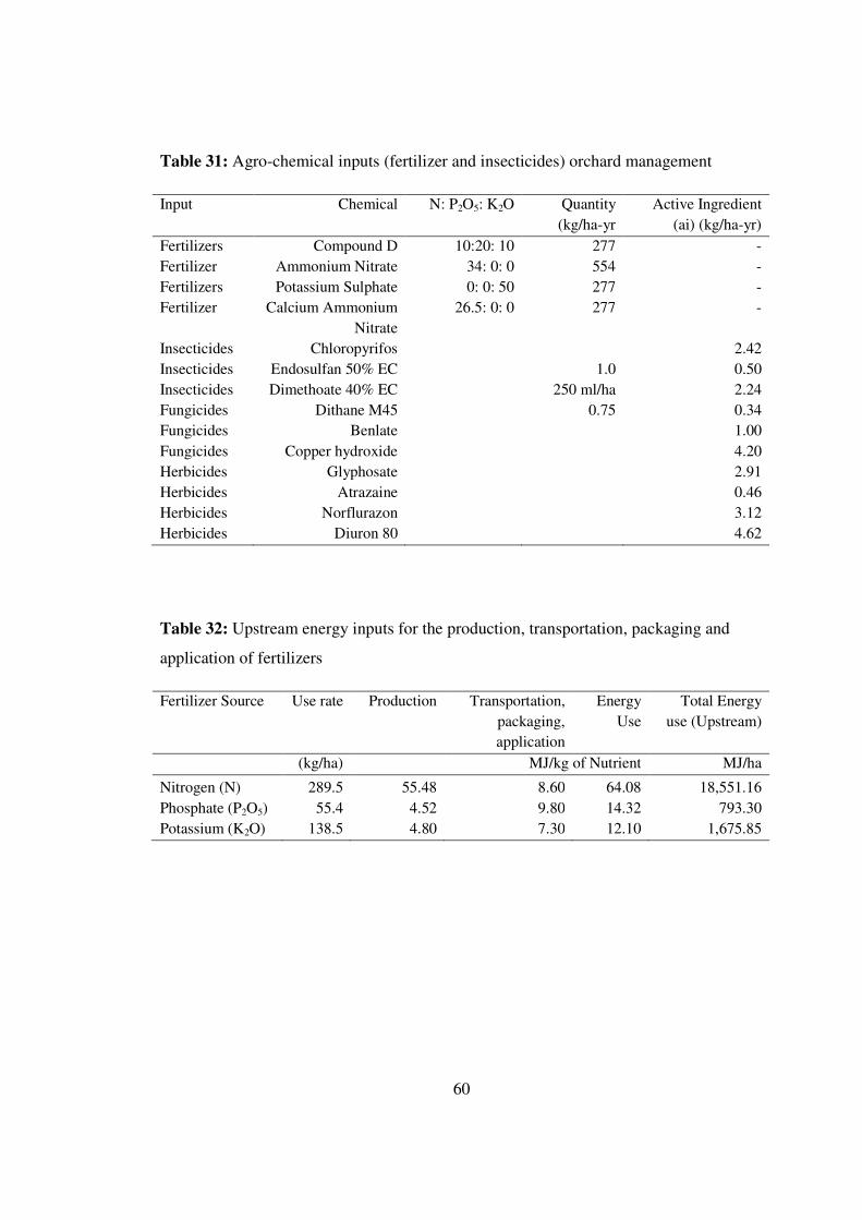
60
Table 31: Agro-chemical inputs (fertilizer and insecticides) orchard management
Input Chemical N: P2O5: K2O Quantity
(kg/ha-yr
Active Ingredient
(ai) (kg/ha-yr)
Fertilizers Compound D 10:20: 10 277 -
Fertilizer Ammonium Nitrate 34: 0: 0 554 -
Fertilizers Potassium Sulphate 0: 0: 50 277 -
Fertilizer Calcium Ammonium
Nitrate
26.5: 0: 0 277 -
Insecticides Chloropyrifos 2.42
Insecticides Endosulfan 50% EC 1.0 0.50
Insecticides Dimethoate 40% EC 250 ml/ha 2.24
Fungicides Dithane M45 0.75 0.34
Fungicides Benlate 1.00
Fungicides Copper hydroxide 4.20
Herbicides Glyphosate 2.91
0.46 Herbicides Atrazaine
Herbicides Norflurazon 3.12
Herbicides Diuron 80 4.62
Table 32: Upstream energy inputs for the production, transportation, packaging and
application of fertilizers
Fertilizer Source Use rate Production Transportation,
packaging,
application
Energy
Use
Total Energy
use (Upstream)
(kg/ha) MJ/kg of Nutrient MJ/ha
Nitrogen (N) 289.5 55.48 8.60 64.08 18,551.16
Phosphate (P2O5) 55.4 4.52 9.80 14.32 793.30
Potassium (K2O) 138.5 4.80 7.30 12.10 1,675.85

61
Table 33: Emissions from production of fertilizer used in orchard management
Nutri
ent
Energy Source
(MJ/ha)
Emission Factor (g/MJ) Total Emissions (g/ha)
CO2 CH4 N2O CO2 CH4 N2O
N Natural
Gas
14,999 11.829 0.633 0.000178 177423.2 9494.367 2.670
Diesel 1,742.8 29.215 0.728 0.000164 50915.9 1268.758 0.286
Electricity 1,545.9 228.464 0.481 0.00290 353189.4 743.5923 4.483
P2O5 Natural
Gas
0.00 11.829 0.633 0.000178 0 0 0.000
Diesel 396.11 29.215 0.728 0.000164 11572.35 288.3681 0.065
Electricity 397.22 228.464 0.481 0.00290 90750.47 191.0628 1.152
K2O Natural
Gas
372.57 11.829 0.633 0.000178 4407.131 235.8368 0.066
Diesel 768.68 29.215 0.728 0.000164 22456.99 559.599 0.126
Electricity 534.61 228.464 0.481 0.00290 122139.1 257.1474 1.550
Sub-Total 832854.5 13038.73 10.398
Source: (Bhat et al., 1994)
Table 34: Volatile organic carbon (VOC) and carbon monoxide (CO) emissions from
fertilizer production
Nutrient Energy Source (MJ/ha), Emissions factor (g/MJ) Emissions (g/ha)
VOC CO VOC CO
N Natural Gas 14,999 0.00672 0.0188 100.7933 281.98
Diesel 1,742.8 0.0131 0.0403 22.83068 70.23
Electricity 1,545.93 0.021 0.0541 32.46453 83.68
P2O5 Natural Gas 0.00 0.00672 0.0188 0 0
Diesel 396.11 0.0131 0.0403 5.189041 15.96323
Electricity 397.22 0.021 0.0541 8.34162 21.49
K2O Natural Gas 372.57 0.00672 0.0188 2.50367 7.00
Diesel 768.68 0.0131 0.0403 10.06971 30.98
Electricity 534.61 0.021 0.0541 11.22681 28.92
Sub-Total 193.4193 540.21
Energy values: Source: (Bhat et al., 1994)

62
Table 35: Energy requirements for the production, formulation, packaging and
distribution of pesticides
Pesticide Production
Energy
(MJ/kg)
Formulation
(MJ/kg)
Packaging
and
Distribution
(MJ/kg)
Total
Energy
(MJ/kg)
Total Energy
(MJ/ha)
Insecticides
Dimethoate 40%
EC
245.06 20 7 272.06 609.41
Chloropyrifos 245.06 20 7 272.06 658.39
Malathion 50% EC 245.06 20 7 272.06 136.03
Fungicides
Benlate 356.39 30 7 393.39 393.39
Copper hydroxide 356.39 30 7 393.39 1,652.24
Dithane M45 356.39 30 7 393.39 133.75
Herbicides
Glyphosate 214.93 10 7 231.93 674.92
Atrazaine 214.93 10 7 231.93 106.69
Norflurazon 214.93 10 7 231.93 723.62
Diuron 80 214.93 10 7 231.93 1,071.52

63
Table 36: Emissions factors and GHG emissions from production of pesticides;
emission factors were multiplied by the energy used in the production of pesticides.
Pesticide Energy Source
(MJ/ha)
Emission Factor (g/MJ) Total Emissions (g/ha)
CO2 CH4 N2O CO2 CH4 N2O
Insecticides
Dimethoate Natural
Gas
609.41 11.83 0.63 0.00018 7208.711 385.75 0.11
Chloropyrifos Natural
Gas
658.39 11.83 0.63 0.00018 7788.095 416.76 0.12
Malathion Natural
Gas
136.03 11.83 0.63 0.00018 1609.099 86.11 0.02
Fungicides
Benlate Natural
Gas
393.39 11.83 0.63 0.00018 4653.41 249.016 0.07
Copper
hydroxide
Natural
Gas
1,652.2 11.83 0.63 0.00018 19544.34 1045.86 0.29
Dithane M45 Natural
Gas
133.75 11.83 0.633 0.00018 1582.129 84.66 0.02
Herbicides
Glyphosate Natural
Gas
674.92 11.83 0.633 0.00018 7983.6287 427.22 0.12
Atrazaine Natural
Gas
106.69 11.83 0.633 0.00018 1262.036 67.53 0.02
Norflurazon Natural
Gas
723.62 11.83 0.633 0.00018 8559.701 458.05 0.13
Diuron 80 Natural
Gas
1,071.52 11.83 0.633 0.00018 12675.01 678.27 0.19
Sub-Total 72866.167 3899.26 1.09

64
Table 37: Volatile organic carbon (VOC) and carbon monoxide (CO) emissions from
production of pesticides
Pesticide Upstream Energy
Source (MJ/ha)
Emissions factor (g/MJ) Emissions (g/ha)
VOC CO VOC CO
Insecticides
Dimethoate Natural
Gas
609.41 0.00672 0.0188 4.095235 11.46
Chloropyrifos Natural
Gas
658.39 0.00672 0.0188 4.424381 12.38
Malathion Natural
Gas
136.03 0.00672 0.0188 0.914122 2.56
Fungicides
Benlate Natural
Gas
393.39 0.00672 0.0188 2.643581 7.39
Copper
hydroxide
Natural
Gas
1,652.24 0.00672 0.0188 11.10305 31.06
Dithane M45 Natural
Gas
133.75 0.00672 0.0188 0.8988 2.51
Herbicides
Glyphosate Natural
Gas
674.92 0.00672 0.0188 4.535462 12.69
Atrazaine Natural
Gas
106.69 0.00672 0.0188 0.716957 2.01
norflurazon Natural
Gas
723.62 0.00672 0.0188 4.862726 13.60
Diuron 80 Natural
Gas
1,071.52 0.00672 0.0188 7.200614 20.14
Sub-Total 41.39493 115.81

65
Table 38: Summary of carbon dioxide equivalent emissions for Plot 1; after conversion
of LCA data to carbon equivalents using the respective global warming potential
Source of emission CO2 CH4 N2O VOC CO gCO2eq/ha
GWP 1 25 298 3.04 1.57
Land Preparation 10,984 292.08 20.37 377.91 6,803.47 45632.1
Cultural operations 519,400 29.2 199.92 309.4 2,126.07 586655.2
Energy for production
of fuels
318,424.6 5446.30 2.56 103.9 314.63 456,464.96
Fertilizers
Energy for production 832,854.5 13,038.7 10.4 193.42 540.21 1163867.1
N2O emissions from
application
0 0 4550 0 0 1355900.0
N2O emissions from
pruning
0 0 121.81 0 0 36299.4
N2O Volatile 0 0 455 0 0 135590.0
N2O leaching 0 0 1051 0 0 313198.0
Pesticides 72,866.17 3899.255 1.1 41.39 115.81 171092.4
Total Emissions of
GHGs
1754529.2 567638.4 191082 1595.10 30017.9 4264699.2
Total Carbon dioxide equivalent emissions (g CO2e/ha) 4,264,699
GWP: (Source: PAS 2050, 2011)
Summary of carbon emissions for high input orchards
The average carbon emissions for the five high input orchards was 4.272 Mg CO2e/ha
per year (Table 39). The five orchards received similar amounts of inputs, but the
difference in application and residue biomass from pruning resulted in different carbon
emissions. The accumulated carbon emissions for the reported 15 years of application is
64.08 Mg CO2e/ha. The carbon emission figures were presented as negative values in
the table.

66
Table 39: Summary of GHG emissions in for the five high-input orchards
Plot Field
Work
Emission
Fuel
Production
Emissions
Fertilizer
Production
Emissions
Fertilizer
Application
Emissions
Pesticide
Production
Emissions
Total
Emissions
(Mg CO2e/ha)
Plot1 -0.632 -0.456 -1.164 -1.841 -0.171 -4.26
Plot 2 -0.635 -0.456 -1.164 -1.845 -0.171 -4.27
Plot 3 -0.638 -0.456 -1.164 -1.85 -0.171 -4.28
Plot 4 -0.639 -0.456 -1.164 -1.849 -0.171 -4.28
Plot 5 -0.636 -0.456 -1.164 -1.845 -0.171 -4.27
Average -0.636 -0.456 -1.164 -1.846 -0.171 -4.272
CARBON EMISSIONS FROM FIVE LOW INPUT ORCHARDS
4.4.2 Emissions determination for Plot 6 orchard
The life cycle analysis for this low input orchard considered carbon emissions from the
inputs of pesticides, electricity and fuel. The pesticides used during the year under
consideration included Malathion 50% EC, Dimethoate 40% EC, Dithane M45 and
Benlate as shown in Table 40. Water was applied to the orchard by way of pumping
from a stream using a 4 HP grid electrical powered pump. Diesel fuel was used in the
initial stage of land preparation. The field was established in 1984 on a cleared land. The
application of water and pesticides to the orchard was continued for a period of 10 years.
A 60 HP tractor was taken to have been used hooked to plow, disc harrow and row disk.
in the initial land preparation. The field was irrigated by pumping water from shallow
well using a 5 horse power pump running with a discharge of 4 litres per second
operated for predetermined period for 13 days in a year at an irrigation interval of two to
three weeks during the dry season. The GHG emissions sources [(i) to (vi)] described in
section 3.2.2 were tabulated and the total GHG emissions calculated for this plot were
summarized as shown in Table 41. This procedure was repeated for the remaining low
in-put orchards.

67
Table 40: The agro-chemical input (fertilizer and pesticides) to the orchard
Input Chemical Quantity
(kg/ha-yr)
Active Ingredient (ai) (kg/ha-yr)
Pesticides Malathion 50% EC 1.0 0.50
Dimethoate 40% EC 250 ml/ha 2.24
Benlate 1.0 1.00
Fungicides Dithane M45 0.75 0.34
Table 41: Summary of GHGs emissions for Plot 6 in Lusaka district
Source of emission CO2 CH4 N2O VOC CO g CO2eq/ha
GWP 1 25 298 1.57 3.04
Land Preparation 6,784 265.33 17.27 333.05 6,110.84 37663.55
Energy for production
of fuels
154,313.2 3379.02 1.011 61.91 189.51 239763.29
N2O emissions from
pruning
0 0 111 0 0 33078.00
N2O emissions from
leaching
0 0 24.9 0 0 7420.20
Pesticides 13618.136 728.74 0.205 7.74 21.64 31975.66
Total Emissions of
GHGs
174715.34 109327.3 46007 632.24 19218.85 349900.70
Total Carbon dioxide equivalent emissions (g CO2e/ha) 349,900.70
4.4.3 Emissions determination for Plot 7 orchard
Plot 7 was small holder relatively low input orchard which was well managed. There
was no use of high level mechanization that was reported in the performance of all unit
operations on the field. All the activities including irrigation, spraying, fertilizer
application and pruning were reported to be done manually. Spraying for control of pests
and diseases was done using a Knapsack sprayer, which is considered carbon emissions
neutral. The agro-chemical inputs applied included urea and mixed fertilizers
(compound D), Malathion 50% EC, Dimethoate 40% EC, Dithane M45 and Benlate as

68
shown in Table 42. The farmer was able to recall the amount of fertilizers applied
consistently over the years as was advised by the Ministry of Agriculture and Livestock
extension staff, but was unable to remember the exact amounts of pesticides in which
case literature and Ministry of Agriculture and Livestock recommendations were used
on the mentioned products. For purposes of this study machinery was assumed to be
used in the initial land preparation. A 60 HP tractor working with a plow and row disk
was used in the calculations. The calculations of the carbon footprints for this orchard
are summarized in Table 43.
Table 42: Agro-chemical inputs to the orchard
Input Chemical Quantity
(kg/ha-yr
Active Ingredient (ai) (kg/ha-
yr)
Fertilizer Compound D 200 -
Fertilizer Urea 200 -
Pesticides Malathion 50% EC 1.0 0.5
Dimethoate 40% EC 250 ml/ha 2.24
Fungicides Dithane M45 0.75 0.34
Fungicides Benlate 1.0 1.0

69
Table 43: Summary of GHG emissions for Plot 7 orchard
Source of emission CO2 CH4 N2O VOC CO gCO2eq/ha
GWP 1 25 298 3.04 1.57
Land Preparation 5,088 384.27 23.2 472.7 8,789.6 49070.94
Energy for production
of fuels
100,406.1 2501.99 0.564 45.02 138.503 163615.67
Fertilizers
Energy for production 313,738.8 4,951.21 4.18 73.2 204.64 439501.75
N2O emissions from
application
0 0 1760 0 0 524480
CO2 emissions from
urea application
314,285.7 0 0 0 0 314285.7
N2O emissions from
pruning
0 0 160.48 0 0 47823.04
N2O Volatile 0 0 1760 0 0 524480
N2O leaching 0 0 432.1 0 0 128765.8
Pesticides 13,429.79 728.626 0.230 7.71 21.53 31791.54
Total Emissions of
GHGs
746948.45 214152. 1233944 939.8 27828.9 2223814.43
Total Carbon dioxide equivalent emissions (g CO2e/ha) 2,223,814.43
4.4.4 Emissions determination for Plot 8 orchard
This is among the oldest orchards included in this study, being planted in 1974. It’s a
small holder orchard. Low inputs were applied for a period of five years from 1976 to
1980 after which the application was stopped after the owner fell ill over an extended
period of time. The applied inputs are targeted at improving fruit yield. Ammonium
nitrate was used to apply nitrate to the plants. Pesticides (Malathion 50% EC,
Dimethoate 40% EC and Dithane M45 were reported to have been used in the control of
pests and diseases (Table 44). Irrigation water was drawn from shallow wells located
within the orchard. The method of drawing water was the use of pump tied to a string,
lowered manually to scoop the water. Initial land preparation was assumed to have been
done using a tractor. The farmer owned a tractor and pairs of oxen for Animal Draft
Power. Land maintenance, replanting and pruning was said to be done by hand. But its
worthy noting that from 1980 to the study date, the orchard was generally left
unattended to. The analysis of the carbon emissions due to agro-chemical manufacture,

70
packaging and distribution and use were tabulated. The summary of emissions was
recorded in Table 45.
Table 44: Agro-chemical inputs to the orchard
Input Chemical Quantity
(kg/ha-yr
Active Ingredient (ai) (kg/ha-
yr)
Fertilizers Ammonium Nitrate 800 -
insecticides Malathion 50% EC 1.0 0.5
insecticides Dimethoate 40% EC 250 ml/ha 2.24
Fungicides Dithane M45 0.75 0.34
Table 45: Summary of GHGs emissions for Plot 8
Source of emission CO2 CH4 N2O VOC CO gCO2eq/ha
GWP 1 25 298 3.04 1.57
Land Preparation 5,088 448.36 26.75 550.45 10,248.3 56287.54
Energy for production
of fuels
100,406.1 2501.99 0.564 45.022 138.50 163615.65
Fertilizers
Energy for production
of fertilizers
546,375.2 10811.1 6.99 146.65 409.50 820210.84
N2O emissions from
application
0 0 4274 0 0 1273652
N2O emissions from
pruning
0 0 187.7 0 0 55934.6
N2O Volatile 0 0 427 0 0 127246
N2O leaching 0 0 1003.8 0 0 299132.4
Pesticides 10399.94 556.53 0.156 5.91 16.53 24419.21
Total Emissions of
GHGs
662,269 14317.98 5927 748.032 10,812.8 2820498.23
Total Carbon dioxide equivalent emissions (g CO2e/ha) 2,820,498.2

71
4.4.5 Carbon emissions determination for Plot 9 orchard
Plot 9 was an orchard only six years old. The orchard had reached bearing age and in
fact was reported to have at one time produced fruits, although at the time of the study
one could easily see that the trees were water stressed and planted in a less productive
environment. There was no irrigation of the crop taking place. The crop had not been
ever irrigated since the time of planting. An attempt was made to try and lay drip liners,
but the project couldn’t be completed. Fertilizer was reported to have been applied only
once during the establishment year at the rate of 100 g per plant per year as shown in
Table 46. The insecticide Malathion 50% EC and the fungicides Dithane M45 and
copper oxyhydroxide were commonly used by most citrus farmers. Knapsack is
common spraying equipment for small scale farmers and was used. The field as noted
above was planed in 2005, but no land use change was done; the field had been planted
to other crops before then. The results of the emissions for this orchard were
summarized in Table 47.
Table 46: Agro-chemical inputs to Plot 9 orchard
Input Chemical Quantity
(kg/ha-yr
Active Ingredient (ai) (kg/ha-
yr)
Fertilizer Compound D 45 -
Pesticides Malathion 50% EC 1.0 0.5
Fungicides Dithane M45 0.75 0.34

72
Table 47: Summary of GHGs emissions for Plot 9 Orchard
Source of emission CO2 CH4 N2O VOC CO gCO2eq/ha
GWP 1 25 298 3.04 1.57
Land Preparation 3,816 107.97 7.43 133.51 2,476.16 16466.53
Energy for production
of fuels
69,432.8 1835.25 0.42 32.22 81.7 115738.16
Fertilizers
Energy for
production
28,217.47 286.74 0.36 5.102 12.72 35539.93
N2O emissions from
application
0 0 70.71 0 0 21071.58
N2O emissions from
pruning
0 0 45.04 0 0 13421.92
N2O Volatile 0 0 7.1 0 0 2115.80
N2O leaching 0 0 26.06 0 0 7765.88
Pesticides 3,047.71 169.69 0.05 1.75 3.99 7319.74
Total Emissions of
GHGs
104513.98 59991.25 46836.66 270.95 7826.69 219439.54
Total Carbon dioxide equivalent emissions (g CO2e/ha) 219,439.54
4.4.6 Carbon emissions determination for Plot 10 Orchard
Plot 10 appeared to have been receiving sufficient care. The orchard was weed free and
apparently disease and pest free. The orchard was planted in 1992. Application of inputs
was done and continued for a period of 16 years. The fertilizers used include urea and
compound D at the rate of 500 g per tree as given in Table 48. The re-currency of pests
and diseases was controlled using the commonly available pesticides Malathion 50%
EC, Dimethoate 40% EC and Dithane M45 (Table 44). Irrigation water was supplied by
a 1 HP submersible pump from a shallow well. The initial land preparation is assumed to
have been done using a 60 HP tractor hooked to implements such as plow and disc
harrow. The calculation procedures outlined for Plot 1 was used to calculate emissions
for this plot and the rest of the calculated carbon emissions were summarized and
recorded in Table 49.

73
Table 48: Agro-chemical inputs to Plot 10
Input Chemical Quantity (kg/ha-
yr
Active Ingredient (ai)
(kg/ha-yr)
Fertilizer Compound D 200 -
Fertilizer Urea 200 -
Pesticides Malathion 50% EC 1.0 0.5
Dimethoate 40% EC 250 ml/ha 2.24
Fungicides Dithane M45 0.75 0.34
Table 49: Summary of GHG emissions for Plot 10 Orchard
Source of emission CO2 CH4 N2O VOC CO gCO2e/ha
GWP 1 25 298 3.04 1.57
Land Preparation 5,088 335.89 20.52 414.04 7,687.76 43621.04
Energy for fuel
production
205,682.32 2723.64 1.9 54.7 163.43 274922.23
Fertilizers
Energy for
production
320,373.7 4949.8 4.01 73.59 205.32 446053.39
N2O emissions from
application
0 0 1760 0 0 524480.00
CO2 emissions from
urea application
314,285.7 0 0 0 0 314285.70
N2O emissions from
pruning
0 0 140.2 0 0 41779.60
N2O Volatile 0 0 176 0 0 52448.00
N2O leaching 0 0 427.5 0 0 127395.00
Pesticides 10399.94 556.53 0.156 5.91 16.53 24419.21
Total Emissions of
GHGs
855829.66 214146 754025 860.7368 24542.04 1849404.2
Total Carbon dioxide equivalent emissions (g CO2e/ha) 1,849,404
Average GHG emissions from the four low input plots
The average carbon emissions for the four (4) low input orchards was 1.81 Mg CO2e/ha
per year (Table 50). Plot 9 was left out from the average on account of young age (six
years) when compared to those in other plots which were all 19 years and above.

74
Biomass accumulation was directly related to the age of the plants and this necessitated
averaging within the age group. Figure 12 shows the average carbon sequestration and
average GHG emissions per level of management-High and low input. Notably the bar
graph shows more average carbon sequestration for the low input than the high input
management level. The average GHG emissions are lower for the low input orchards
than the high inputs. The carbon emission figures were presented as negative values in
the tables and figures below.
Table 50: Summary of carbon emissions for the four (4) low input orchards
Plot Field
Work
Emission
Fuel
Production
Emissions
Fertilizer
Production
Emissions
Fertilizer
Application
Emissions
Pesticide
Production
Emissions
Total
Emissions
(Mg CO2e/ha)
Plot 6 -0.04 -0.24 -0.0 -0.04 -0.03 -0.35
Plot 7 -0.05 -0.16 -0.44 -1.54 -0.03 -2.22
Plot 8 -0.06 -0.16 -0.82 -1.76 -0.02 -2.82
Plot 10 -0.04 -0.27 -0.45 -1.06 -0.02 -1.85
Average -0.0475 -0.2075 -0.4275 -1.1 -0.025 -1.81

75
Figure 12: Average carbon sequestration and emissions by management level
The accumulated emissions over the reported period of external input application for the
low input are shown in Table 51. Small holder farmers did not report continuous use of
inputs through out the life of the orchards. For some periods the orchards were left with
minimum attention during which carbon emissions due to external inputs was negligible.
Table 51: Weighted average accumulated emissions from the low input orchards
Plot Total Emissions
(Mg CO2e/ha)
Reported period of
application (years)
Accumulated emissions
(Mg CO2e/ha)
Plot 6 -0.35 10.00 -3.50
Plot 7 -2.22 13.00 -28.91
Plot 8 -2.82 5.00 -14.10
Plot 9 -0.22 2.00 -0.44
Plot 10 -1.85 16.00 -29.59
Average -1.81 -19.03
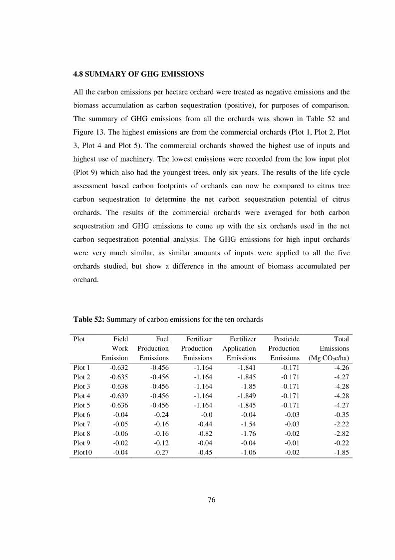
76
4.8 SUMMARY OF GHG EMISSIONS
All the carbon emissions per hectare orchard were treated as negative emissions and the
biomass accumulation as carbon sequestration (positive), for purposes of comparison.
The summary of GHG emissions from all the orchards was shown in Table 52 and
Figure 13. The highest emissions are from the commercial orchards (Plot 1, Plot 2, Plot
3, Plot 4 and Plot 5). The commercial orchards showed the highest use of inputs and
highest use of machinery. The lowest emissions were recorded from the low input plot
(Plot 9) which also had the youngest trees, only six years. The results of the life cycle
assessment based carbon footprints of orchards can now be compared to citrus tree
carbon sequestration to determine the net carbon sequestration potential of citrus
orchards. The results of the commercial orchards were averaged for both carbon
sequestration and GHG emissions to come up with the six orchards used in the net
carbon sequestration potential analysis. The GHG emissions for high input orchards
were very much similar, as similar amounts of inputs were applied to all the five
orchards studied, but show a difference in the amount of biomass accumulated per
orchard.
Table 52: Summary of carbon emissions for the ten orchards
Plot Field
Work
Emission
Fuel
Production
Emissions
Fertilizer
Production
Emissions
Fertilizer
Application
Emissions
Pesticide
Production
Emissions
Total
Emissions
(Mg CO2e/ha)
Plot 1 -0.632 -0.456 -1.164 -1.841 -0.171 -4.26
Plot 2 -0.635 -0.456 -1.164 -1.845 -0.171 -4.27
Plot 3 -0.638 -0.456 -1.164 -1.85 -0.171 -4.28
Plot 4 -0.639 -0.456 -1.164 -1.849 -0.171 -4.28
Plot 5 -0.636 -0.456 -1.164 -1.845 -0.171 -4.27
Plot 6 -0.04 -0.24 -0.0 -0.04 -0.03 -0.35
Plot 7 -0.05 -0.16 -0.44 -1.54 -0.03 -2.22
Plot 8 -0.06 -0.16 -0.82 -1.76 -0.02 -2.82
Plot 9 -0.02 -0.12 -0.04 -0.04 -0.01 -0.22
Plot10 -0.04 -0.27 -0.45 -1.06 -0.02 -1.85

77
Figure 13: Total GHG emissions for the ten orchards in various districts of Lusaka
province
Table 53: Summary of carbon sequestration, GHG emissions and net carbon
sequestration for the ten orchards
Plot Carbon
Sequestration
(Mg CO2e/ha)
Total Carbon
Emissions
(Mg CO2e/ha)
Net Carbon
Sequestration
(MgCO2e/ha)
Plot 1 71.1 -63.9 7.20
Plot 2 77.8 -64.05 13.75
Plot 3 85.5 -64.2 21.30
Plot 4 84.8 -64.2 20.60
Plot 5 78.3 -64.05 14.25
Plot 6 64.6 -3.50 61.10
Plot 7 93.6 -28.86 64.74
Plot 8 109.2 -14.1 95.10
Plot 9 26.3 -0.44 25.86
Plot10 81.8 -29.6 52.20

78
Figure 14: Carbon sequestration, GHG emissions and net carbon sequestration. Carbon
emissions were indicated as negative (middle bar) and the carbon sequestration was
denoted by positive values. The net carbon sequestration was the difference between
carbon sequestration and carbon emissions (right bar) were positive for all the ten (10)
orchards.
The average carbon sequestration, GHG emissions and net carbon sequestration were as
shown in Table 54, Table 55 and Table 56.
Table 54: Average carbon sequestration results for different levels of management
Management
Level
Biomass
(Mg/ha)
Carbon Stock
(Mg C/ha)
Carbon Eq. (Mg
CO2e/ha)
Annual CO2e Increment
(Mg CO2e/ha)
High Input 43.36 21.66 79.5 7.62
Low input 47.63 23.80 87.30 9.35

79
Table 55: Average GHG emissions for different levels of management
Manage
ment
Level
Field
Work
Emission
Fuel
Production
Emissions
Fertilizer
Production
Emissions
Fertilizer
Application
Emissions
Pesticide
Production
Emissions
Total
Emissions
(Mg CO2e/ha)
High
input
-0.636 -0.456 -1.164 -1.846 -0.171 -4.272
Low
input
-0.0475 -0.2075 -0.4275 -1.1 -0.025 -1.81
Table 56: Net carbon sequestration potential of orchard per management level
Management
Level
Biomass-
Average
(Mg
CO2e/ha)
LCA
(MgCO2e/ha)
Period of
Input
application
(Years)
GHG
Emissions
Accumulation
(Mg CO2e/ha)
Net Carbon
Sequestration
(Mg CO2e/ha)
High Input 79.49 -4.28 15.00 -64.08 15.42
Low Input 87.3 -1.81 - -19.03 68.27

80
Figure 15: Net carbon sequestration by management level. The average carbon
sequestration for high input (left bar) orchards is lower than that for low inputs. Net
carbon sequestration for both management levels was postive and there was higher
average net carbon sequestration for low input orchards than for the high input orchards.

81
Figure 16: The average distribution of carbon emissions by contribution per activity
under high (a) and low (b and c) in-puts systems showing the differences of contribution
of fertilizer production and application to total GHG emissions between high and low
input orchard management.

82
Figure 17: Emissions distribution by activity-low input (d to f) orchards. For low input
orchards where fertilizer application is low, the contribution of GHG emissions from
fertilizer production and application is also low.

83
Chapter 5
DISCUSSION
Carbon sequestration
The citrus tree biomass accumulation from the planting date to the date of the study was
determined by the use of allometric equations developed for citrus, dry tropical forest
and other agro-forestry and shade trees which relate the biophysical parameter such as
plant diameter to biomass. A total of fourteen orchards were visited out of which ten
were used in the analysis for this study. The average carbon sequestration for four low
input orchards was high at 87.3 Mg CO2e/ha as compared to 79.5 Mg CO2e/ha for high
input or commercial orchards. The carbon sequestration of citrus did not appear to
increase with the increase in external inputs (regression coefficient was 0.44), but
appeared to increase with the age of citrus trees (regression coefficient was 0.55) and
other factors such as soil fertility which were not considered in this study.
A wide range of diameters at breast height (DBH, in this case at 30 cm above ground)
were measured in each plot or orchard. The smallest DBH recorded was 5.8 cm from
Plot 9 (Mean DBH was 9.94 cm) which had six year old plants and the highest recorded
was 27.1 cm from Plot 8 (Mean DBH was 23.65 cm) which was the oldest orchard at 37
years. The highest population density of 450 citrus plants per hectare was observed in
Plots 1 and 6 which were among the plots from the small holder or low input growers
and the lowest density was 277 plants per hectare among the commercial growers. The
plots with the highest population density recorded the lowest biomass accumulation of
14.3 and 35.2 Mg/ha for plots Plot 9 and plot 6 respectively. This result is in agreement
with Juwarkar et al., (2011) who also found that in the natural forest, trees with higher
population density had smaller DBH but accumulated lower biomass compared to those
with larger DBH.

84
The calculated biomass per tree ranged from 23.99 kg/tree from Plot 9 to 190.67 kg/tree
from Plot 8 and this is equivalent to carbon sequestration of 26.3 and 109.2 Mg CO2e/ha
for plots Plot 9 and Plot 8 respectively. The average biomass per tree for high input plots
was found to be 156.5 kg/tree. The average carbon sequestration for the five commercial
plots was 79.57 Mg CO2e/ha and the average carbon sequestration for low input was
87.3 Mg CO2e/ha. The value of carbon sequestration for the low input management
systems was higher than that for the high input management, a finding was not expected,
but could be explained from spatial location differences in terms of soil fertility and also
the age of the trees as noted above. The citrus trees are said to increase trunk diameter at
the rate of 0.78 cm annually, (UNFCCC/NUCC, 2011), during their active growing
period before reaching the optimum tree size. From this annual increment in diameter,
the annual biomass change converted to carbon dioxide equivalents, has been calculated
(using equation 4) to range from 5.3 to 10.3 Mg CO2e/ha.
The calculated biomass per tree was comparable with what Morgan et al. (2006) found
in a study to determine biomass and Nitrogen distribution of sweet oranges using a
Destructive Method to determine dry weight tree biomass of citrus, (Citrus sinensis L.
Osbeck). In their study the dry weight per tree was found to be about 100 kg/tree and the
fresh weight ranged from 120 to 194 kg/tree, (Morgan et al., 2006) and other studies
have also shown similar results of dry weight biomass of about 100 kg/tree.
The carbon stock recorded in this study was lower than what other studies have recorded
in natural forests. This is mainly on account of different species of trees; citrus spp are
generally small to medium trees reaching only up to a maximum height of 13 m while
forest trees can reach the height of 22 m, (Manner et al., 2006 and Juwarkar et al.,
2011).
The allometric equation which was developed by Scroth (Scroth et al., 2002) had limited
use becuase the upper limit DBH of 17 cm was far exceeded by most citrus trees in the
study. This probably explains why the average biomass per tree found in this study was
slightly higher than what Morgan et al. (2006) found in their study, whose age range for
the citrus was 3 to 15 years.

85
The biomass accummulation was seen to be affected by application of external inputs as
well as natural factors such as climate and georaphical location. Several complex and
interacting factors affect citrus growth. These include air and soil temperature, soil
moisture conditions, soil pH and sunshine. The average rainfall and soil moisture
condition is very important in semi-arid environments. Since all the orchards studied are
located in the same agro-ecological region, the effect of air temperature, sunshine and
wind speed on the differences in biomass accummulation may be generally the same for
all the orchards. The effect of local soil moisture conditions and pH and plant nutrient
status for each particular orchard may have a profound effect on biomass
accummulation. Like noted in sections 4.2.2, 4.2.3 and section 4.2.5 above, citrus trees
in Plot 7, Plot 8 and Plot 10 which are located in the fertile flood plain, despite being
low input (small holder) orchards recorded marked biomass accummulation even higher
than commercial orchards (Plot 1) planted in other regions. The large increase in
biomass accummulation by trees in plots 7, 8 and 10 may have been due to the
availability of sufficient soil moisture during the most part of the dry season, which was
also supplemented by irrigation with water drawn from shallow wells. Although citrus
are shallow rooted trees, it is possible that they were able to access flood plain moisture
from the soil during the most part of the dry season. Plot 9 which was located on a
higher land, despite being an old orchard, the biomass accummulation was low; partly
because no fertilizers were reported to have been used and also due to insufficient soil
moisture during the dry season. The reported irrigation during the dry season may have
not been sufficient. The biomass accummulation was observed to be increasing linearly
with the increase in DBH. The regression analysis showed the regression coefficient
ranged from 0.883 to 0.996 which is a strong correlation.
Life cycle assessment
Life Cycle Assessment was a process used to evaluate the total environmental impact of
agro-chemical inputs from manufacture to application and use on the orchards in order
to determine the GHG emissions attributed to citrus orchard biomass production. The
second part of this study determined the total GHG emissions using the life cycle

86
approach of carbon foot-printing of inputs and outputs at the farm/orchard level. The
GHG emissions of citrus orchard production were calculated in conformity with PAS
2050: 2011 recommendations. All carbon (or GHG) emissions were considered negative
emissions and carbon sequestration as positive values. The output was expressed as tree
biomass accumulated in a hectare of citrus trees. Two different production systems were
considered; the high input which were commercial orchard production and the low input
practiced by small holder citrus producers. For the high input the average GHG
emissions was 4.272 Mg CO2e/ha while that for low input was 1.81 Mg CO2e/ha. The
GHG emissions from the individual orchards from the low input management systems
ranged from 0.22 to 2.82 Mg CO2e/ha. The major source of GHG emissions from the
commercial orchards was from the production and application of chemical fertilizers
which supply the essential plant elements of N, P2O5 and K2O. The other major
contribution to carbon emissions was the field work operations and electricity consumed
in the running of irrigation water pumps. Small holder orchards had the GHG emissions
also mainly coming from fertilizer production and application and emissions due to crop
residues where applicable and from electricity use.
In the high input orchard 43 percent of GHG emissions were due to fertilizer
application-the release of nitrous oxide from fertilizer applied as nitrogen and also from
urea application. The other greenhouse gas emissions were due to upstream emissions
from the production and delivery of fertilizers (27%). The other major contributing
factor to the GHG emissions were emissions attributed to field work; fifteen percent
(15%) for high input orchards and three percent (3%) for low inputs, and that associated
with fuel and electricity production and use. Field work emissions were as a result of
burning fossil fuels in farm machinery. Where there was no application of fertilizers, the
bulky of emissions shifted to the production and use of fuel and electricity (68%)
followed by emissions due to crop residue and field work at 12 and 11 percent (%)
respectively. The emissions from the application of nitrogen fertilizer also include
emissions estimated from the decomposing organic matter (from pruning material left as
crop residue on fields). The GHG emissions from the small holder orchards were much
smaller as compared to the emissions from the commercial orchards.

87
Both the commercial and small holder farmers may have opportunities to reduce their
farm GHG emissions by reducing emissions from fertilizer application and from field
work operations by implementing measures such as reducing fertilizer inputs and use of
smaller tractors with lower fuel consumption and use of renewable energy. The reported
amount of nitrogen fertilizer use was high and a reduction in the amount of nitrogen
fertilizer applied would result in significant reduction in emissions.
The results of this study were similar to studies conducted in other countries. A study
conducted in Egypt reported a baseline scenario (without composting) carbon emissions
of 3.2 Mg CO2e/ha for citrus production, (Luske, 2010). This value falls within the range
determined for this study and compares well with other studies done for similar
perennial crops like Apples (Page, 2011). Page, (2011) in a study conducted in New
Zealand found carbon emissions of 2.8 and 3.8 Mg CO2e/ha from energy use only in a
Kiwifruit and Apple organic orchard production systems respectively. Another study
done in the USA on citrus found similar amount of emissions from inputs, 8.4 Mg
CO2e/ha, although slightly high on account of heavy use of inputs and highly
mechanized orchards which included even conveyor belts to transport harvested fruits,
(EPA, 2010).
The variation in the reported GHG emissions per hectare of citrus could first and
foremost partly be explained in terms of the differences in the levels of external inputs
and management. Differences in methodologies and assumptions made can also lead to
differences in results. The other explanation would be due to the use of emissions factors
that were not developed for the local environment. The emission factors and the GREET
Model: 2011 used in this study were developed for use in the United States and Europe.
Apparently there were no country-specific emission factors for inputs and processes in
Zambia. This lead to the use of emission factors and models which were derived mostly
for European systems and American systems such as for the production, packaging and
transportation of fertilisers and pesticides which may not accurately reflect the situation
in Zambia. In conformity with the British Standards’ PAS 2050, (2011), the carbon foot-
printing applied in this study did not consider the orange fruits as carbon sequestration
product and carbon sequestration and emissions from the soil was excluded due to

88
uncertainty of the impact of agricultural technologies used in land management, (PSA:
2050, 2011). Most of the orchards where the study was done were established before 31st
December 1989 and therefore, emissions from land use change were not considered and
there were no reports of expanding the orchards into natural forests.
The data collected from the farmers/managers had some gaps that were filled by use of
secondary data from literature. For some orchards which were established many years
ago and without proper records, it was not possible to establish the exact amount of
external inputs that were used. The small holder farmers were unable to remember the
exact amount of pesticides. This necessitated the use of the standard values from
literature.
Net carbon sequestration
Net carbon sequestration can be determined by caculating the difference between
biomass accumulation and the total accumulated GHG emissions over the life span of
the orchard. Alternatively, annual biomass increment (carbon sequestration) can be
compared with the annual GHG emissions, (Page, 2011). Farmers reported that they had
been applying the inputs annually to the orchards for different periods ranging from two
years for plot 9 to 15 years for high input plots and 16 years for Plot 10. The resulting
accumulative GHG emissions ranged from 3.5 Mg CO2 e/ha for Plot 9 representing low
input plots to 64.2 Mg CO2 e/ha and high inputs. The resulting net carbon sequestration
ranged from 15.35 Mg CO2e/ha for high input orchards to 68.27 Mg CO2e/ha for low
input orchards. Alternatively, from the average annual GHG emissions of 4.3 Mg
CO2e/ha and annual carbon sequestration of 7.62 Mg CO2e/ha, the net carbon
sequestration was calculated as 3.32 Mg CO2e/ha for high input orchards. The low input
orchards had a higher average annual carbon sequestration of 9.35 Mg CO2e/ha and a
lower avarage annual GHG emissions of 1.81 Mg CO2e/ha, the net carbon emission for
the low input orchards was determined to be 7.54 Mg CO2e/ha. The net carbon
sequestration potential for high input orchard mangement systems could become

89
negative after a contionous annual application of inputs of similar amounts as the ones
used in this analysis beyond the fruit bearing age.
Both of the methods for determining the net carbon sequestration have their own
weaknesses. The total accumulated GHG emissions were calculated by assuming that
the external inputs used in a typical year as reported by the farmers/managers, the exact
same amounts were repeated every other typical year for the period of application
reported. On the other hand, the annual biomass increment (annual carbon sequestration)
was calculated using equation which is an exponential function which gives higher
values for higher DBH.

90
Chapter 6
6.0 CONCLUSIONS AND RECOMMENDATIONS
6.1 Conclusion
Citrus trees sequester carbon and the net carbon sequestration potential by citrus (Citrus
sinensis (L.) Oesbeck) is higher for low external input management systems than higher
external input management systems (commercial production). Although the carbon stock
in citrus trees is lower than that found in the natural forest, clearly citrus trees do
sequester carbon in biomass, and can remain so for well over 50 years. The carbon
sequestration potential of citrus partly depended on age. Older plants sequestered more
carbon than younger plants. The productivity could be enhanced by proper management;
well managed orchards sequestered more carbon than those that did not receive good
care.
The application of agro-chemical inputs and use of mechanized technologies on orchards
results in carbon emissions. This study has established that GHG emissions do not
exceed carbon sequestration for both high and low input citrus orchard management
systems. Low input citrus orchards are carbon sinks. High input orchards remain carbon
sinks until the carbon emissions exceed carbon sequestration due to continuous
application of agro-chemical inputs beyond the optimum fruit bearing age. This means,
therefore, that growing of citrus especially with low input management systems offers an
opportunity to mitigate climate change by reducing CO2 from the atmosphere through
carbon sequestration in citrus biomass. The results showed that continuous application
of inputs-fertilizer, pesticides and water (except where water is applied manually),
beyond the bearing period of citrus resulted in net carbon emissions becoming negative,
otherwise judicious application of inputs to citrus plantations does not give net negative
greenhouse gas emissions.

91
6.2 Recommendations
The UNFCCC’s Kyoto protocol CDM meant to help developing countries to come up
with sustainable life improvement projects that which remove or sequester carbon in
exchange for developed countries to have the right to emit similar amount of carbon,
needs to be relooked at or reviewed. On the face value, such schemes do give the same
benefits to the developed and developing countries. The value of a ton of carbon
sequestered in forests in terms of improving the lives of poor people living in developing
countries, may not be the same as a tone of carbon emitted through industrial activities
and effect it has on the lives of citizens of developed countries. This could be taken into
account when negotiating and developing policies on the implementation of CDM
programmes.
In this study four (4) different equations were used and the biomass determined from the
average, and thus, there was generally little variation. In future it would be worthwhile
to conduct studies but using Destructive Methods and comparing the reliability.
Such data can be used to formulate more allometric equations that incorporate local
environment variability. Accurately determining GHG emissions and carbon
sequestration is vital to forest and agro-forestry management. But this is difficult to
achieve without locally developed carbon emission factors and allometric equations for
calculating aboveground biomass. It is recommended that comprehensive studies could
be carried out to develop country specific and local allometric equations and GHG
emission factors, which could be applied in the assessment of live biomass held by both
the natural and agro-forests.

92
Chapter 7
REFERENCES
1http://coloradocollege.edu/dept/ev/courses/EV212/Block5_2002/Combust.html
ADHIKARI M., 2005. A non-destructive approach for quantitative assessment of tree
resources outside the forest. Msc thesis, International Institute for Geo-Information
Science and Earth Observation, Netherlands.
ANDREAE M. O. and Merlet P., 2001. Emission of Trace Gases and Aerosols from
Biomass Burning, Global Biogeochemical Cycles 15 (4) 955-966.
ANL, 2009. Argonne National Laboratory, The Greenhouse Gases, Regulated
Emissions, and Energy Use in Transportation (GREET) Model, GREET 1.8c.0, Fuel
Specs, US Department of Energy.
BHAT, M. G., English, B. C., Turhollow A. F. and Nyangito H. O., 1994. Energy in
Synthetic Fertilizers and Pesticides: Revisited, Oak Ridge National Laboratory (ORNL),
US Department of Energy, ORNL/Sub/90-99732/2.
BOCKEL L. Smith G., Marjory B., Martial B., Marianne T., Henry M., Giacomo
B., 2011. Mainstreaming carbon balance appraisal of agriculture projects and policies:
Tool for measuring Carbon-Balance in Ex-ante Project- Programme Impact Appraisal”,
A Policy brief, FAO, EASYPOOL
BROWN S., Gillespie A. J. R. and Lugo E. A., 1989. Biomass estimation methods for
tropical forests with applications to forest inventory data. Society of American Foresters.
Forest Science Vol. 35 No. 4
BROWN, S. 1997. Estimating biomass and biomass change of tropical forests: a primer.
FAO Forestry Paper 134. Rome. Italy.
BROWN, S. 2002. Measuring carbon in forests: current status and future challenges.
Environmental Pollution.
CARBON TRUST. 2011. Conversion factors. Energy and conversions. Defra/DECC.
Fact sheet
COLE C. V., Duxbury J., Freney J., Heinemeyer O., Minami K., Mosier A.,
Paustian K., ROSENBURG N., Sampson N., Sauerbeck D. and Zhao Q., 1997.
Global estimats of potential mitigation of greenhouse gas emissions by agriculture. Nutr.
Cycl. Agroecosyst.

93
DALGAARD T., Halberg N. and Porter J. R., 2001. A Model for Fossil Energy Use
in Danish Agriculture used to Compare Organic and Conventional farming, Agr.
Ecosyst. Environ.
De GIER, A., 1999. Woody biomass assessment in woodlands and shrub-lands, off-
forest tree resources of Africa, Arusha, Tanzania.
De GIER, A., 2003. A new approach to woody biomass assessment in woodlands and
shrub-lands. In: P. Roy (Ed), Geo-informatics for Tropical Ecosystems, India, pp. 161-
198.
DOUGLAS L., 2004. Global warming, Facts on File, Inc., New York.
EKVALL, T. and Weidema B. P., 2004. System Boundaries and Input Data in
Consequential Life Cycle Inventory Analysis, Int J LCA Vol. 9(3).
ENVIRONMENTAL PROTECTION AGENCY, 2004. US Exhaust and Crankcase
Emission Factors for on road Engine Modeling--Compression-Ignition, EPA420-P-04-
009, April 2004.
ENVIRONMENTAL PROTECTION AGENCY, 2005. Conversion Factors for
Hydrocarbon Emission Components, EPA420-R-05-015, December 2005, NR-002c.
ENVIRONMENTAL PROTECTION AGENCY, 2010. Analysis of Innovative
Feedstock Sources and Production Technologies for Renewable Fuels Final Report.
EPA: XA-83379501-0
FAO LocClim, 2002. Local Climate estimator, www.fao.or/sd/2002/EN1803a_en_html
FUTCH, Steve; Brlansky, Ron; Irey, Mike, and Weingarten, Shawron, 2008.
Detection of Greening in Sprouts from Citrus Tree Stumps, International Research
Conference on Huanglongbing (RCHLB) Proceedings, December, 2008.
GRAHAM R. L, Wright L. L, Turhollow A. F., 1992. The potential for short rotation
woody crops to reduce U.S. CO2 emissions. Climate Change.
GREEN M., 1987. Energy in pesticide manufacture, distribution, and use. Energy in
Plant Nutrition and Pest Control ed. Z.R. Helsel. New York: Elsevier, pp. 165-96.
HAIRIAH, K., Sitompul, S.M., Noordwijk, Van M. and Palm, C., 2001. Methods for
sampling carbon stocks above and below ground. ASB Lecture Note 4B. ICRAF,
Indonesia.

94
HARLEY I. M., Bucker S. R., Smith V. E., Ward D. and Elevitch C. R., 2006.
Species Profiles for Island Agroforestry. Permanent Agricultural Resources, Halualoa,
Hawai.
HEIJUNGS, R., 1996. Life Cycle Assessment: What it is and how to do It. United
Nations Environment Programme; Paris.
HINSON, Roger A.; Boudreaux, James E.; Vaughn, Alan, 2006. Projected Costs of
Establishing and Operating a Citrus Grove, Louisiana State University Agricultural
Center, A.E.A. Information Series No. 140. August 2006.
IPCC, 2001. Intergovernmental Panel on Climate Change: The Scientific Basis.
University of Cambridge, Cambridge, UK.
IPCC, 2005. IPCC good practice for LULUCF sector. Intergovernmental Panel on
Climate Change. University of Cambridge press, Cambridge, UK.
IPCC, 2006a. Energy, Volume 2 in 2006 IPCC Guidelines for National Greenhouse Gas
Inventories, NGGIP Publications.
IPCC, 2006b. Agriculture, Forestry and Other Land Use, Volume 4. IPCC Guidelines
for National Greenhouse Gas Inventories, NGGIP Publications.
IPCC, 2007. Summary for Policymakers. Climate Change: The Physical Basis.
Contribution of Working Group I to the Fourth Assessment Report of the
Intergovernmental Panel on Climate Change. Cambridge University Press. Cambridge.
United Kingdom and New York, NY, USA.
ISAAC M. E., Timmer V. R. and Quashie-Sam S. J., 2007. Nutrient Cycling in
Agroecosystems (formerly Fertilizer Research), Springer Science + Business Media
B.V. 10.1007/s10705-006-9081-3
IS0 (14040), 1997. International Standard Organization. Environmental Management -
Life Cycle Assessment - Principles and Framework, First edition.
JANA B. K., Biswas S., Majumder M., Roy P. K. and Mazumdar A., 2009. Carbon
sequestration rate and aboveground biomass carbon potential of four young species,
Journal of Ecology and Natural Environment Vol. 1(2), pp. 015-024, May, 2009
JOHNSON J. M., Franzleubbers A. J., Weyers S. L. and Reicosky, 2007.
Agriculture opportunities to mitigate greenhouse gas emissions. Environ. Pollut. 150:
107-124
JUWARKAR A. A., Varghese A. O., Singh S. K., Aher V. V. and Thawale P. R.,
2011. Carbon sequestration potential in aboveground biomass of natural reserve forest of
central India. International Journal of Agriculture: Research and Review. Volume 1 (2).

95
KERCKHOFFS L. H. J. and Reid J. B., 2007. Carbon sequestration in the standing
biomass of orchard crops in New Zealand. New Zealand Institute for Crops and Food
Research Ltd, Hastings, New Zealand.
KETTERINGS, Q. M., Coe, R., Noordwijk, M., Ambagau, Y. and Palm C.A. 2001.
Reducing uncertainty for predicting above-ground tree biomass in mixed secondary
forests. Forest ecology and management.
LAL R., Kimble J. M., Follett R. F., Cole C. V., 1998. The Potential of U.S. cropland
to sequester and mitigate the greenhouse effect. Boca Raton, FL: Lewis Publishers.
LAL R. 2004. Carbon emission from farm operations. ELSEVIER. Environment
international. USA
LASCO R. D., Pulhin F. B., Sanchez P. A J., Villamor G. B. and Villegas K. A. L.,
2008. Climate Change and Forest Ecosystems in the Philippines: Vulnerability,
Adaptation and Mitigation. Journal of Environmental Science and Management 11(1):1-
14 . ISSN 0119-1144
LOSI, C.J., Siccama, T.G., Condit, R. and Morales, J.E., 2003. Analysis of
alternative methods for estimating carbon stock in young tropical plantations. Forest
Ecology and Management, 184(1-3): 355-368.
LUSKE B., 2010. Reduced GHG emissions due to compost production and compost use
in Egypt, Comparing two scenarios, Louis Bolk Institute.
MANNER I H., Richard S. B., Virginia E. S., Deborah W. and Craig R. E., 2006.
Species Profiles for Pacific Island Agro-forestry.
MARBLE S. C., Prior S. A., Runion G. B., Torbert H. A., Gillian C. H. and Fain B.
G., 2011. The Importance of Determining Carbon Sequestration and Greenhouse Gas
Mitigation Potential in Ornamental Horticulture, HORTSCIENCE Vol. 46(2), Auburn,
USA.
MASERA O. R., Garza-Caligaris J.F., Kanninen M., Karjalainen T., Liski J.,
Nabuurs G. J., Pussinen A., de Jong B. H. J., Mohren G.M. J., 2003. Modeling
carbon sequestration in afforestation, agroforestry and forest management projects: the
CO2FIX V.2 approach; Elsevier Science, Ecological modeling 164
MILLENNIUM Ecosystem Assessment. 2005. Ecosystems and human well-being:
Synthesis. Island Press, W. A.
MINISTRY of Agriculture and Cooperatives/FAO, 2007. Farm Management
Resource Guide, Lusaka, Zambia

96
MORGAN K. T., Scholberg J. M. S., Obreza, T. A., Wheaton T. A., 2006. Size,
Biomass and Nitrogen Relationships with Sweet orange Tree Growth, J AMER. SOC.
HORT. SCI 131.
MUDAHAR M. S. and Hignett T. P., 1987. Energy Requirements, Technology, and
Resources in the Fertilizer Sector. Energy in Plant Nutrition and Pest Control. Z.R.
Helsel. New York: Elsevier, pp. 25-62.
MURARO, Ronald P., 2008a. Summary of 2007-2008 Citrus Budget for the Central
Florida (Ridge) Production Region, Citrus Research and Education Center, Institute of
Food and Agricultural Sciences (IFAS) Extension, University of Florida, September
2008.
NAIR, P.K.R., Kumar, B.M. and Nair, V.D. 2009. Agroforestry as a strategy for
carbon sequestration. Journal of Plant Nutrition and Soil Science.
NAMDARI M., Kangarshahi A. A. and Amiri A. N. 2011. Modeling energy flow for
orange production in Iran. International Journal of Plant, Animal and Environmental
Sciences. Volume 1: Issue 1.
NOORDWIJK M. V., Rahayu S., Hairia K. H., Farida Y. C. W. A and Verbist B.,
2002. Carbon stock assessment for a forest-to-coffee conversion landscape in Sumber-
Jaya (Lampung, Indonesia): from allometric equations to land use change analysis . Vol.
45 Supp. SCIENCE IN CHINA (Series C).
OECD, 1999. Environmental Indicators for Agriculture; Vol. 1. Concepts and
Framework, OECD, Paris France.
OECD/IEA, 2011. CO2 emissions from fuel combustion highlights. International
Energy Agency 9 rue de la Federation 75739 Paris Cedex 15, France
OZKAN B., Akcaoz H. and Karadeniz F. 2003. Energy requirement and economic
analysis of citrus production in Turkey. ELSEVIER. Energy Conversion and
Management.
PAGE G., 2011. Modeling of Carbon Footprints of Organic Orchard Production
Systems to Address Carbon Trading: An Approach Based on Life Cycle Assessment,
HORTSCIENCE Vol. 46(2)
PAS: 2050, 2011. Publicly available specification for the assessment of the life cycle
greenhouse gas emissions of goods and services. BSI, ISBN 978 0 580 71382 8 ICS
13.310; 91.190
PHAT, N.K., Knorr, W. and Kim, S., 2004. Appropriate measures for conservation of
terrestrial carbon stocks--Analysis of trends of forest management in Southeast Asia.
Forest Ecology and Management, 191(1-3).

97
PLASSMANN K., Norton A., Attarzadeh N., Jensen . P. M., Brenton P. and Jones-
Edwards G. 2010. Methodological complexities of carbon footprinting: a sensitivity
analysis of key variables in a developing country context. ELSEVIER. Environmantal
Science and Policy. UK.
SCHROTH G., D’Angelo S. A., Teixeira W.G., Haag D. and Lieberei R., 2002.
Conversion of secondary forest to agroforestry and monoculture plantations in
Amazonia: consequences for biomass, litter and soil carbon stock after 7 years. Forest
Ecology and MANAGEMENT 163: 131-150.
SEGURA, M. and Kanninen, M., 2005. Allometric Models for tree volume and total
abovegound biomass in a tropical humid forest in Costa Rica. Biotropica, 37(1): 2-8.
SHEPHERD M., Pearce B., Cormack B., Philipps L., Cuttle S. and Bhogal A., 2003.
An Assessment of the Environmental Impact of Organic farming; A Review of Defra-
Funded Project OF0405
STOLZE M., Piorr A., Haring A. and Dabbert S., 2000. The Environmental Impacts
of Organic Farming in Europe, Organic Farming in Europe: Economics and Policy,
Department of Farm Economics, University of Hohenheim, Stuttgart, Germany
TIMOTHY P., Walker S. and Brown S., 2005. Source book for Land Use, Land-Use
Change and Forestry Projects, Winrock International.
TORIO D. D., 2007. Modeling canopy density variations from remotely sensed data:
Implication on monitoring floristic and macro-benthic properties of mangrove
ecosystems; International Institute for Geo-Information Science and Earth Observation,
Enschede, The Netherlands.
UNITED NATIONS, 1998. Kyoto protocol to the United Nations Framework
convention on climate change, Kyoto, Japan.
UNFCCC/CCNUCC, 2011. Project Design Document Form for Afforestation and
Reforestation Project Activities (CDM-AR-PDD) - Version 05 1/100; CDM – Executive
Board
VERMER C. C. and de Meer V. J. P., 2010. Carbon pools in tropical peat forest:
Towards a reference value for forest biomass carbon in relatively undisturbed peat
swamp forests in southeast Asia. Wageningen Alterra, Alterra-Report 2108,
Wageningen.
WATSON, R.T., Dixon, J.A., Hamburg, S.P., Janetos, A.C. and Moss, R.H., 1998.
Protecting Our Planet Securing Our Future – Linkages among Global Environmental
Issues and Human Needs, United Nations Environment Programme, U.S. National
Aeronautics and Space Administration and The World Bank.

98
WEST O. T and Marland G. 2002. A synthesis of carbon sequestration, carbon
emissions, and net carbon flux in agriculture: comparing tillage practices in the United
States. ELSEVIER, Agriculture Ecosystems and Environment. USA
WOOD S. and Cowie A., 2004. A review of greenhouse gas emission factors for
Fertilizer Production. Research and Development Divison, State Forests of New South
Wales. Cooperative Research Centre for Greenhouse Accounting. For IEA Bio-energy
Task 38.
ZIANIS, D. and Mencuccini, M., 2004. On simplifying allometric analyses of forest
biomass. Forest Ecology and Management.
ZEMEK O. J., 2009. Biomass and carbon stocks inventory of perennial vegetation in
the Chieng Khoi Watershed, M.sc. thesis, University of Hohenheim, NW VIET NAM

99
APPENDICES
APPENDIX A
Appendix A1: Citrus tree biomass calculation and results for Plot 1
Name of Farm: A1
Province: Lusaka
Plot Size: A1 1,800 sqm
Citrus Varieties: Washington Navel, Valencia
Biomass Biomass Biomass Biomass Average
Tree No. Tree Age DBH D (m) BA (cm2) Eq1 kg/Tr Eq2 kg/Tr Eq3 kg/Tr Eq4 kg/Tr
1 35 14 0.14 153.94 48.49 31.12 51.74 61.97 48.33
2 35 20.6 0.206 333.29 151.82 103.94 122.10 151.82 132.42
3 35 15.7 0.157 193.59 66.64 43.58 66.76 80.84 64.45
4 35 16.8 0.168 221.67 80.46 54.07 77.60 94.59 76.68
5 35 20.1 0.201 317.31 143.40 96.24 115.61 143.40 124.67
6 35 20.1 0.201 317.31 143.40 96.24 115.61 143.40 124.67
7 35 22.9 0.229 411.87 194.07 143.45 154.49 194.07 171.52
8 35 20.1 0.201 317.31 143.40 96.24 115.61 143.40 124.67
9 35 19.6 0.196 301.72 135.26 88.87 109.32 135.26 117.18
10 35 21.1 0.211 349.67 160.50 111.97 128.79 160.50 140.44
11 35 15.6 0.156 191.13 65.46 42.71 65.81 79.65 63.41
12 35 20.1 0.201 317.31 143.40 96.24 115.61 143.40 124.67
13 35 21 0.21 346.36 158.74 110.34 127.44 158.74 138.82
14 35 22.4 0.224 394.08 184.38 134.31 147.10 184.38 162.54
15 35 12 0.12 113.10 31.49 22.64 36.73 43.34 33.55
16 35 11 0.11 95.03 24.52 21.04 30.27 35.41 27.81
17 35 15.9 0.159 198.56 69.02 45.35 68.66 83.25 66.57
18 35 22.4 0.224 394.08 184.38 134.31 147.10 184.38 162.54
19 35 24.1 0.241 456.17 218.49 166.57 173.07 218.49 194.15
20 35 16.1 0.161 203.58 85.70 47.18 70.59 85.70 72.29
21 35 20.1 0.201 317.31 143.40 96.24 115.61 143.40 124.67
22 35 23.3 0.233 426.38 202.03 150.97 160.56 202.03 178.90
23 35 19.5 0.195 298.65 133.67 87.44 108.08 133.67 115.71
24 35 18.9 0.189 280.55 124.32 79.13 100.83 124.32 107.15
25 35 22.6 0.226 401.15 188.23 137.93 150.03 188.23 166.10
26 35 18 0.18 254.47 97.64 67.61 90.46 111.01 91.68
27 35 17 0.17 226.98 83.17 56.18 79.67 97.23 79.06
28 35 15.4 0.154 186.27 63.16 41.04 63.95 77.30 61.36
29 35 20.5 0.205 330.06 150.11 102.38 120.79 150.11 130.85
30 35 19.6 0.196 301.72 135.26 88.87 109.32 135.26 117.18
31 35 22.1 0.221 383.60 176.02 128.97 142.75 178.71 156.61
32 35 14.8 0.148 172.03 56.57 36.40 58.55 70.49 55.50
33 35 21.2 0.212 352.99 155.89 113.61 130.15 162.27 140.48
34 35 19.5 0.195 298.65 133.67 87.44 108.08 133.67 115.71
35 35 16 0.16 201.06 70.24 46.25 69.62 84.47 67.65
36 35 23 0.23 415.48 198.00 145.31 156.00 196.05 173.84
37 35 21.7 0.217 369.84 171.29 122.02 137.07 171.29 150.42
38 35 20.3 0.203 323.65 146.74 99.28 118.19 146.74 127.74
39 35 26.7 0.267 559.90 277.11 222.03 217.34 277.11 248.40
40 35 21.9 0.219 376.68 174.98 125.47 139.90 174.98 153.83
41 35 15 0.15 176.71 58.71 37.88 60.32 72.72 57.41
42 35 20.1 0.201 317.31 143.40 96.24 115.61 143.40 124.67
43 35 19.1 0.191 286.52 127.39 81.84 103.21 127.39 109.96
44 35 15.6 0.156 191.13 65.46 42.71 65.81 79.65 63.41
45 35 17.1 0.171 229.66 84.54 57.26 80.71 98.56 80.27
46 35 16.8 0.168 221.67 80.46 54.07 77.60 94.59 76.68
47 35 25.8 0.258 522.79 255.92 202.04 201.39 255.92 228.82
48 35 18.8 0.188 277.59 122.80 77.79 99.64 122.80 105.76
Plot Biomass 6253.25 4370.81 5221.27 6479.43 5581.19
Expansion Factor 5.56 5.56 5.56 5.56 5.56
Aboveground Biomass/ha 34740.29 24282.30 29007.03 35996.81 31006.61
Belowground Biomass/ha 8685.07 6070.57 7251.76 8999.20 7751.65
Total Biomass/ha 43425.37 30352.87 36258.79 44996.01 38758.26
Carbon/ha (Total Biomas/2ha) 21712.68 15176.44 18129.40 22498.01 19379.13
Carbon Equivalents (kg CO2eq.) 79620.41 55651.99 66480.49 82500.19 71063.27
5% of Biomass Prunned 1737.01 1214.11 1450.35 1799.84 1550.33
Tree Maintenance/Replacement @4% 1737.01 1214.11 1450.35 1799.84 1550.33

100
Appendix A2: Citrus tree biomass calculation and results for Plot 2
Name of Farm: A2
Province Lusaka
Plot Size: A2 1,800 sqm
Citrus Varieties: Washington Navel, Valencia
Biomass Biomass Biomass Biomass Average
Tree No. Tree Age DBH D (m) BA (cm2) Eq1 kg/Tr Eq2 kg/Tr Eq3 kg/Tr Eq4 kg/Tr kg/Tree
1 35 13 0.13 132.73 39.45 26.02 43.88 52.18 40.38
2 35 19.1 0.19 286.52 127.39 81.84 103.21 127.39 109.96
3 35 21.1 0.21 349.67 160.50 111.97 128.79 160.50 140.44
4 35 25.5 0.26 510.71 249.07 195.56 196.22 249.07 222.48
5 35 18 0.18 254.47 111.01 67.61 90.46 111.01 95.03
6 35 20.1 0.20 317.31 143.40 96.24 115.61 143.40 124.67
7 35 22.1 0.22 383.60 178.71 128.97 142.75 178.71 157.28
8 35 14 0.14 153.94 48.49 31.12 51.74 61.97 48.33
9 35 22.8 0.23 408.28 192.11 141.60 153.00 192.11 169.71
10 35 21.8 0.22 373.25 173.13 123.74 138.48 173.13 152.12
11 35 23.4 0.23 430.05 204.05 152.88 162.09 204.05 180.77
12 35 23.8 0.24 444.88 212.23 160.64 168.32 212.23 188.35
13 35 21 0.21 346.36 158.74 110.34 127.44 158.74 138.82
14 35 23 0.23 415.48 196.05 145.31 156.00 196.05 173.35
15 35 20.3 0.20 323.65 146.74 99.28 118.19 146.74 127.74
16 35 19.3 0.19 292.55 130.51 84.61 105.63 130.51 112.82
17 35 18.6 0.19 271.72 119.79 75.16 97.30 119.79 103.01
18 35 14.4 0.14 162.86 52.43 33.63 55.09 66.15 51.82
19 35 22.1 0.22 383.60 178.71 128.97 142.75 178.71 157.28
20 35 20.2 0.20 320.47 145.07 97.75 116.90 145.07 126.20
21 35 19.7 0.20 304.81 136.87 90.32 110.56 136.87 118.66
22 35 20.4 0.20 326.85 148.42 100.82 119.48 148.42 129.29
23 35 18.3 0.18 263.02 115.35 71.32 93.85 115.35 98.97
24 35 21 0.21 346.36 158.74 110.34 127.44 158.74 138.82
25 35 17.6 0.18 243.28 105.38 62.86 86.05 105.38 89.92
26 35 24.9 0.25 486.95 235.68 182.88 186.10 235.68 210.09
27 35 14.6 0.15 167.42 54.48 34.98 56.80 68.30 53.64
28 35 16.7 0.17 219.04 79.13 53.04 76.58 93.29 75.51
29 35 20.5 0.21 330.06 150.11 102.38 120.79 150.11 130.85
30 35 24.1 0.24 456.17 218.49 166.57 173.07 218.49 194.15
31 35 20.3 0.20 323.65 146.74 99.28 118.19 146.74 127.74
32 35 22.8 0.23 408.28 192.11 141.60 153.00 192.11 169.71
33 35 21 0.21 346.36 158.74 110.34 127.44 158.74 138.82
34 35 20.1 0.20 317.31 143.40 96.24 115.61 143.40 124.67
35 35 25 0.25 490.87 237.89 184.97 187.77 237.89 212.13
36 35 18.1 0.18 257.30 112.45 68.83 91.58 112.45 96.33
37 35 21.6 0.22 366.44 169.47 120.31 135.67 169.47 148.73
38 35 21 0.21 346.36 158.74 110.34 127.44 158.74 138.82
39 35 20.5 0.21 330.06 150.11 102.38 120.79 150.11 130.85
40 35 22.3 0.22 390.57 182.48 132.52 145.64 182.48 160.78
41 35 24.2 0.24 459.96 220.60 168.57 174.67 220.60 196.11
42 35 19.2 0.19 289.53 128.95 83.22 104.42 128.95 111.38
43 35 21.3 0.21 356.33 164.05 115.27 131.52 164.05 143.72
44 35 17.6 0.18 243.28 105.38 62.86 86.05 105.38 89.92
45 35 19.3 0.19 292.55 130.51 84.61 105.63 130.51 112.82
46 35 21.7 0.22 369.84 171.29 122.02 137.07 171.29 150.42
Plot Biomass 6943.14 4872.10 5627.07 7011.06 6113.34
Expansion Factor 5.56 5.56 5.56 5.56 5.56
Aboveground Biomass/ha 38572.99 27067.21 31261.50 38950.33 33963.01
Belowground Biomass/ha 9643.25 6766.80 7815.37 9737.58 8490.75
Total Biomass/ha 48216.24 33834.02 39076.87 48687.92 42453.76
Carbon/ha (Total Biomas/2ha) 24108.12 16917.01 19538.44 24343.96 21226.88
Carbon Equivalents (kg CO2eq.) 88404.48 62034.67 71647.44 89269.29 77838.97
5% of Biomass Prunned 1928.65 1353.36 1563.07 1947.52 1698.15
Tree Maintenance/Replacement @4% 1928.65 1353.36 1563.07 1947.52 1698.15

101
Appendix A3: Citrus tree biomass calculation and results for Plot 3
Name of Farm: A3
Province: Lusaka
Plot Size: A3 1,980 sqm
Citrus Varieties: Washington Navel, Valencia
Biomass Biomass Biomass Biomass Average
Tree No. Tree Age DBH D (m) BA (cm2) Eq1 kg/Tr Eq2 kg/Tr Eq3 kg/Tr Eq4 kg/Tr kg/Tree
1 35 23.5 0.24 433.74 206.08 154.81 163.64 206.08 182.65
2 35 19.6 0.20 301.72 135.26 88.87 109.32 135.26 117.18
3 35 30.1 0.30 711.58 365.95 304.25 283.70 365.95 329.96
4 35 22.0 0.22 380.13 176.84 127.21 141.32 176.84 155.55
5 35 16.7 0.17 219.04 79.13 53.04 76.58 93.29 75.51
6 35 30.6 0.31 736.97 381.14 317.99 294.97 381.14 343.81
7 35 14.0 0.14 153.94 48.49 31.12 51.74 61.97 48.33
8 35 16.2 0.16 206.12 72.70 48.12 71.57 86.94 69.83
9 35 19.6 0.20 301.72 135.26 88.87 109.32 135.26 117.18
10 35 16.8 0.17 221.67 80.46 54.07 77.60 94.59 76.68
11 35 19.2 0.19 289.53 128.95 83.22 104.42 128.95 111.38
12 35 15.6 0.16 191.13 65.46 42.71 65.81 79.65 63.41
13 35 21.8 0.22 373.25 173.13 123.74 138.48 173.13 152.12
14 35 18.3 0.18 263.02 115.35 71.32 93.85 115.35 98.97
15 35 18.1 0.18 257.30 112.45 68.83 91.58 112.45 96.33
16 35 22.1 0.22 383.60 178.71 128.97 142.75 178.71 157.28
17 35 17.4 0.17 237.79 102.62 60.57 83.90 102.62 87.43
18 35 23.8 0.24 444.88 212.23 160.64 168.32 212.23 188.35
19 35 18.3 0.18 263.02 115.35 71.32 93.85 115.35 98.97
20 35 21.1 0.21 349.67 160.50 111.97 128.79 160.50 140.44
21 35 23.6 0.24 437.44 208.12 156.74 165.19 208.12 184.54
22 35 23.0 0.23 415.48 196.05 145.31 156.00 196.05 173.35
23 35 23.4 0.23 429.93 203.98 152.82 162.04 203.98 180.70
24 35 31.7 0.32 787.11 411.38 345.05 317.36 411.38 371.29
25 35 22.8 0.23 408.28 192.11 141.60 153.00 192.11 169.71
26 35 16.5 0.17 213.82 90.72 51.03 74.55 90.72 76.76
27 35 17.9 0.18 251.65 109.59 66.40 89.35 109.59 93.73
28 35 16.2 0.16 206.12 86.94 48.12 71.57 86.94 73.39
29 35 17.1 0.17 229.66 98.56 57.26 80.71 98.56 83.77
30 35 14.0 0.14 153.94 48.49 31.12 51.74 61.97 48.33
31 35 13.6 0.14 145.27 44.74 28.88 48.51 57.94 45.02
32 35 19.8 0.20 309.11 139.11 92.35 112.30 139.11 120.72
33 35 17.0 0.17 226.98 83.17 56.18 79.67 97.23 79.06
34 35 14.6 0.15 167.42 54.48 34.98 56.80 68.30 53.64
35 35 19.7 0.20 304.81 136.87 90.32 110.56 136.87 118.66
36 35 29.1 0.29 663.40 337.37 278.12 262.43 337.37 303.82
37 35 20.3 0.20 323.65 146.74 99.28 118.19 146.74 127.74
38 35 19.4 0.19 295.59 132.08 86.02 106.85 132.08 114.26
39 35 23.8 0.24 444.88 212.23 160.64 168.32 212.23 188.35
40 35 29.9 0.30 701.72 360.08 298.91 279.33 360.08 324.60
41 35 22.9 0.23 411.87 194.07 143.45 154.49 194.07 171.52
42 35 26.7 0.27 558.91 276.54 221.49 216.91 276.54 247.87
43 35 30.2 0.30 715.00 367.99 306.10 285.21 367.99 331.83
44 35 20.2 0.20 320.47 145.07 97.75 116.90 145.07 126.20
45 35 20.0 0.20 314.16 141.75 94.74 114.34 141.75 123.15
46 35 20.6 0.21 333.29 151.82 103.94 122.10 151.82 132.42
47 35 20.7 0.21 336.54 153.53 105.52 123.42 153.53 134.00
48 35 20.0 0.20 314.16 141.75 94.74 114.34 141.75 123.15
49 35 15.6 0.16 191.13 65.46 42.71 65.81 79.65 63.41
50 35 13.1 0.13 134.78 40.30 26.45 44.64 53.12 41.13
51 35 21.6 0.22 366.44 169.47 120.31 135.67 169.47 148.73
52 35 18.3 0.18 263.02 115.35 71.32 93.85 115.35 98.97
Plot Biomass 8301.99 6041.29 6743.67 8453.75 7385.17
Expansion Factor 5.05 5.05 5.05 5.05 5.05
Aboveground Biomass/ha 41929.25 30511.54 34058.92 42695.73 37298.86
Belowground Biomass/ha 10482.31 7627.89 8514.73 10673.93 9324.71
Total Biomass/ha 52411.56 38139.43 42573.65 53369.66 46623.57
Carbon/ha (Total Biomas/2ha) 26205.78 19069.71 21286.83 26684.83 23311.79
Carbon Equivalents (kg CO2eq.) 96096.59 69928.64 78058.80 97853.27 85484.32
5% of Biomass Prunned 2096.46 1525.58 1702.95 2134.79 1864.94
Tree Maintenance/Replacement @4% 2096.46 1525.58 1702.95 2134.79 1864.94
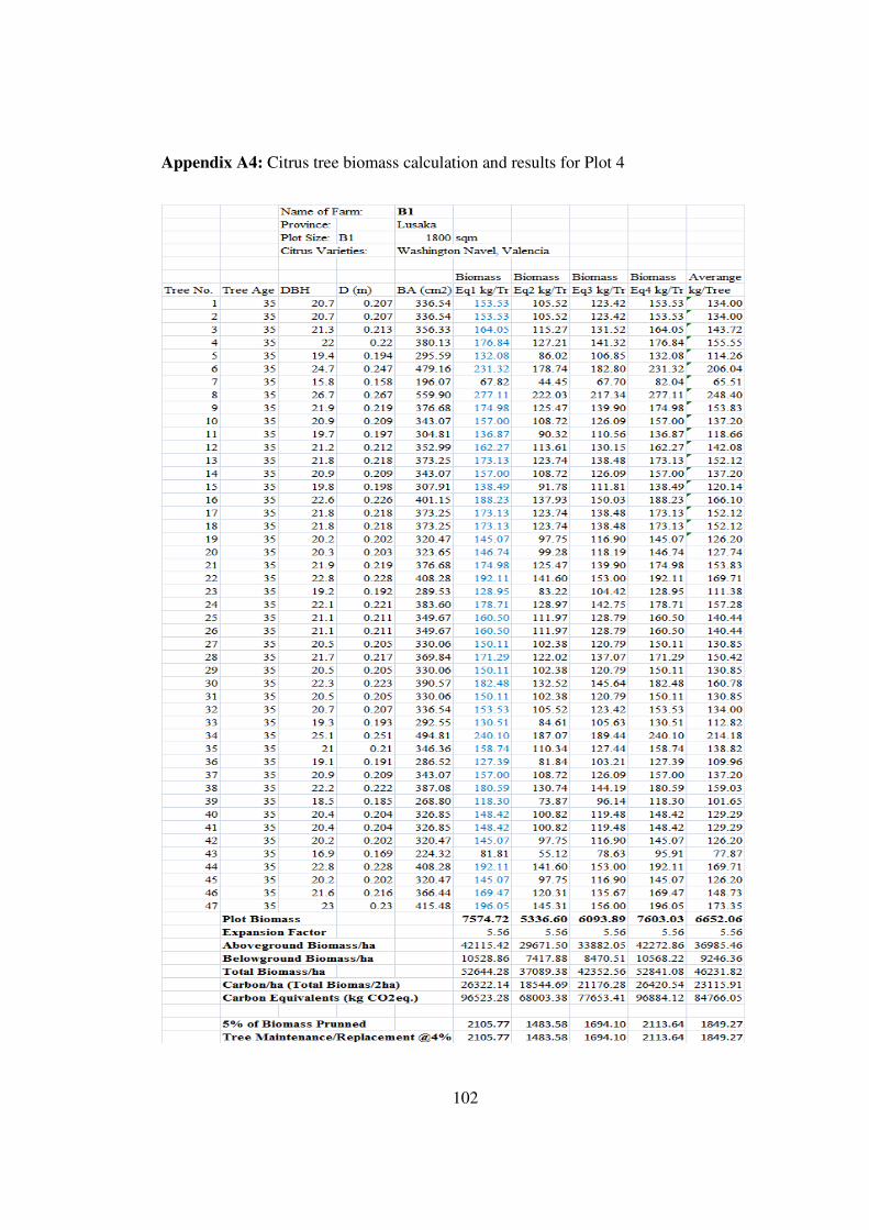
102
Appendix A4: Citrus tree biomass calculation and results for Plot 4

103
Appendix A5: Citrus tree biomass calculation and results for Plot 5

104
Appendix A6: Citrus tree biomass calculation and results for Plot 6
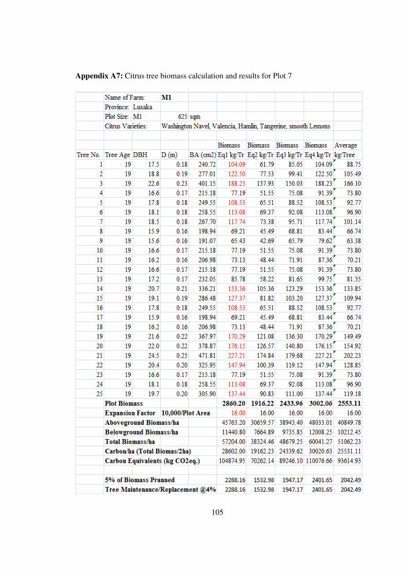
105
Appendix A7: Citrus tree biomass calculation and results for Plot 7

106
Appendix A8: Citrus tree biomass calculation and results for Plot 8

107
Appendix A9: Citrus tree biomass calculation and results for Plot 9

108
Appendix A10: Citrus tree biomass calculation and results for Plot 10

109
APPENDIX B
Appendix B1: GREET model 2011 upstream energy and carbon emissions results
Vehicle Technologies, Light-Duty Trucks 2: Well-to-Pump Energy Consumption and Emissions
(Btu or grams per mmBtu of Fuel Available at Fuel Station Pumps)
Year: 1990
CA
RF
G
Co
mp
ress
ed
Na
tura
l G
as,
NA
NG
LN
GV
: D
ed
ica
ted
, N
A N
G
LP
GV
: D
ed
ica
ted
Na
ph
tha
, n
NA
NG
FC
V:
Me
OH
, n
NA
NG
De
di.
Me
OH
V
eh
icle
: M
90
, n
NA
N
G
CID
I V
eh
icle
: D
ME
, n
NA
NG
CID
I V
eh
icle
: F
T1
00
, n
NA
NG
Ele
ctr
icit
y
(tra
nsp
ort
ati
on
)
Total Energy 255,495 187,400 254,612 164,273 806,956 714,878 617,799 635,641 803,341 1,848,283
WTP Efficiency 79.6% 84.2% 79.7% 85.9% 55.3% 58.3% 61.8% 61.1% 55.5% 35.1%
Fossil Fuels 216,099 176,375 253,097 162,071 806,148 713,708 616,202 634,492 802,523 1,607,762
Coal 35,276 53,921 7,408 10,786 3,951 5,726 7,816 5,620 4,001 1,176,333
Natural Gas 112,193 112,816 232,238 107,108 777,741 667,429 561,682 594,255 776,922 311,039
Petroleum 68,630 9,638 13,451 44,177 24,456 40,553 46,704 34,617 21,599 120,390
CO2 (w/ C in VOC & CO) 16,088 12,480 15,163 12,314 34,022 30,378 27,747 27,821 30,822 241,029
CH4 135.565 667.821 604.837 303.186 769.014 723.154 612.713 691.071 768.501 507.615
N2O 2.371 0.188 0.324 0.185 0.178 0.493 0.441 0.189 0.173 3.060
GHGs 20,184 29,232 30,381 19,949 53,300 48,603 43,196 45,154 50,086 254,631
VOC: Total 28.699 7.088 7.654 10.757 32.767 27.330 27.334 14.026 13.857 22.115
CO: Total 24.138 19.786 24.824 21.877 43.144 55.543 49.302 52.276 42.555 57.106
NOx: Total 63.665 51.226 76.992 61.466 108.878 154.549 138.140 124.891 103.067 502.754
PM10: Total 14.440 10.631 2.822 5.048 15.814 17.013 15.354 15.367 15.661 333.296
PM2.5: Total 5.811 3.295 1.707 2.530 14.916 15.749 13.536 14.091 14.775 88.879
SOx: Total 47.271 46.565 18.833 33.163 37.380 44.289 43.199 46.432 36.373 1184.290
VOC: Urban 16.536 0.207 0.134 2.239 13.428 9.150 10.346 1.165 0.891 1.538
CO: Urban 5.801 0.657 0.653 2.604 0.656 1.297 1.881 1.029 0.574 9.036
NOx: Urban 13.887 3.453 4.326 7.095 3.319 6.487 7.364 5.011 2.626 85.630
PM10: Urban 3.138 0.125 0.099 1.201 0.118 0.220 0.604 0.178 0.099 3.315
PM2.5: Urban 1.538 0.077 0.084 0.611 0.085 0.164 0.346 0.128 0.069 1.878
SOx: Urban 15.332 6.248 0.783 6.463 1.494 2.288 4.031 2.261 1.403 205.037

110
Appendix B2: GREET model 2011 upstream energy and carbon emissions results
Vehicle Technologies, Light-Duty Trucks 2: Well-to-Pump Energy Consumption and Emissions
(Btu or grams per mmBtu of Fuel Available at Fuel Station Pumps)
Year: 2004
Ba
seli
ne
CG
an
d R
FG
CA
RF
G
Co
mp
ress
ed
Na
tura
l G
as,
NA
NG
LN
GV
: D
ed
ica
ted
, N
A N
G
LP
GV
: D
ed
ica
ted
Na
ph
tha
, n
NA
NG
FC
V:
Me
OH
, n
NA
NG
De
di.
Me
OH
V
eh
icle
: M
90
, n
NA
N
G
CID
I V
eh
icle
: D
ME
, n
NA
NG
CID
I V
eh
icle
: F
T1
00
, n
NA
NG
Ele
ctr
icit
y
(tra
nsp
ort
ati
on
)
Total Energy 210,584 224,315 181,472 232,111 160,285 766,579 654,640 573,423 602,835 762,961 1,656,935
WTP Efficiency 82.6% 81.7% 84.6% 81.2% 86.2% 56.6% 60.4% 63.6% 62.4% 56.7% 37.6%
Fossil Fuels 194,459 188,719 170,965 230,810 158,396 765,822 653,584 569,644 601,770 762,195 1,436,648
Coal 18,526 21,077 49,798 6,165 8,966 3,584 5,010 7,474 5,045 3,629 1,044,032
Natural Gas 102,363 100,769 113,305 211,575 112,166 738,070 608,458 515,940 562,429 737,255 313,993
Petroleum 73,570 66,873 7,862 13,071 37,264 24,168 40,116 46,230 34,296 21,310 78,623
CO2 (w/ C in VOC & CO) 15,655 13,663 11,918 13,781 11,530 31,619 26,777 24,830 25,843 28,419 222,202
CH4 128.120 126.994 663.153 590.935 337.766 751.832 697.569 593.476 677.247 751.325 493.220
N2O 0.877 1.878 0.186 0.292 0.180 0.175 0.477 0.548 0.187 0.170 2.982
GHGs 19,119 17,397 28,552 28,641 20,028 50,467 44,359 39,831 42,829 47,253 235,421
VOC: Total 27.464 27.755 6.842 6.972 10.717 31.936 25.769 26.078 13.259 13.191 20.451
CO: Total 17.022 16.181 15.645 19.035 16.756 34.053 42.394 37.755 38.355 33.487 53.824
NOx: Total 55.154 47.127 40.809 57.822 47.877 88.708 121.622 109.468 102.188 85.343 368.290
PM10: Total 8.420 8.977 9.770 2.378 4.201 16.806 17.946 16.202 16.941 16.641 308.338
PM2.5: Total 4.347 4.269 3.000 1.472 2.389 16.077 16.955 14.650 15.914 15.913 82.393
SOx: Total 32.962 30.871 35.951 16.729 28.324 36.055 42.161 40.476 44.773 35.047 828.306
VOC: Urban 15.581 16.471 0.202 0.092 1.970 13.373 9.016 10.216 1.103 0.858 1.469
CO: Urban 3.758 4.951 0.634 0.548 1.804 0.417 0.823 1.359 0.623 0.343 9.700
NOx: Urban 9.546 11.876 2.677 3.064 4.994 2.379 4.374 5.320 3.752 1.986 61.889
PM10: Urban 1.858 2.518 0.117 0.086 0.803 0.156 0.262 0.554 0.242 0.137 3.148
PM2.5: Urban 1.066 1.411 0.074 0.077 0.473 0.133 0.225 0.379 0.207 0.116 1.807
SOx: Urban 8.980 11.702 4.372 0.523 4.120 1.295 1.946 3.232 1.967 1.207 142.258

111
APPENDIX C
Appendix C1: Booking form for aboveground biomass determination

112
Appendix C2: Booking form for external input determination