DI

SC

US

SI

ON

P

AP

ER

S

ER

IE

S

Forschungsinstitut zur Zukunft der ArbeitInstitute for the Study of Labor

Estimation of Productivity in Korean Electric Power Plants: A Semiparametric Smooth Coefficient Model

IZA DP No. 7277

March 2013

Almas HeshmatiSubal C. KumbhakarKai Sun

Estimation of Productivity in Korean

Electric Power Plants: A Semiparametric Smooth Coefficient Model

Almas Heshmati Sogang University

and IZA

Subal C. Kumbhakar Binghamton University

Kai Sun

Aston Business School, Aston University

Discussion Paper No. 7277 March 2013

IZA

P.O. Box 7240 53072 Bonn

Germany

Phone: +49-228-3894-0 Fax: +49-228-3894-180

E-mail: iza@iza.org

Any opinions expressed here are those of the author(s) and not those of IZA. Research published in this series may include views on policy, but the institute itself takes no institutional policy positions. The IZA research network is committed to the IZA Guiding Principles of Research Integrity. The Institute for the Study of Labor (IZA) in Bonn is a local and virtual international research center and a place of communication between science, politics and business. IZA is an independent nonprofit organization supported by Deutsche Post Foundation. The center is associated with the University of Bonn and offers a stimulating research environment through its international network, workshops and conferences, data service, project support, research visits and doctoral program. IZA engages in (i) original and internationally competitive research in all fields of labor economics, (ii) development of policy concepts, and (iii) dissemination of research results and concepts to the interested public. IZA Discussion Papers often represent preliminary work and are circulated to encourage discussion. Citation of such a paper should account for its provisional character. A revised version may be available directly from the author.

IZA Discussion Paper No. 7277 March 2013

ABSTRACT

Estimation of Productivity in Korean Electric Power Plants: A Semiparametric Smooth Coefficient Model

This paper analyzes the impact of load factor, facility and generator types on the productivity of Korean electric power plants. In order to capture important differences in the effect of load policy on power output, we use a semiparametric smooth coefficient (SPSC) model that allows us to model heterogeneous performances across power plants and over time by allowing underlying technologies to be heterogeneous. The SPSC model accommodates both continuous and discrete covariates. Various specification tests are conducted to compare performance of the SPSC model. Using a unique generator level panel dataset spanning the period 1995-2006, we find that the impact of load factor, generator and facility types on power generation varies substantially in terms of magnitude and significance across different plant characteristics. The results have strong implication for generation policy in Korea as outlined in this study. JEL Classification: C14, C23, C51, D24, L25, L94 Keywords: semiparametric estimation, smooth varying-coefficient model,

electricity generation, generator level panel data Corresponding author: Almas Heshmati Department of Economics Sogang University Room K526 Sinsu-dong #1, Mapo-gu Seoul 121-742 Korea E-mail: heshmati@sogang.ac.kr

2

1. Introduction Semiparametric and nonparametric estimation techniques have in recent years attracted much attention from applied researchers (Li and Racine, 2007 and 2010). Their attractiveness is attributed to their flexibility in capturing heterogeneous responsiveness of decision making units with minimum distributional assumptions. Robinson (1988) and Stock (1989) are prime examples of semiparametric and nonparametric models where the functional form of the nonparametric part is not specified. Fan and Li (1996) and Park et al. (1998) provide empirical panel data examples of semiparametric approach, while the time series STAR model version of the smooth coefficient models introduced by Chen and Tsay (1993) and Hastie and Tibshirani (1993) suggest ways to estimate the unknown time variant smooth coefficient functions.

The semiparametric models are generalized in Li et al. (2002) in the context of production function to include a semiparametric smooth coefficient model formulation estimated via kernel method. In such a model the input coefficients are specified as unknown smooth functions of firm’s R&D input. The model follows the generalized knowledge production function of Griliches (1979, 1986). In an application based on Chinese industry data, Li et al. (2002) find the semiparametric model is more flexible than a parametric model. In addition it requires smaller sample size to obtain reliable estimation compared to its non-parametric counterpart. The issue of regional heterogeneity and impact of R&D on productivity of high tech industry at the provincial level in China is investigated by Zhang et al. (2012) using a semiparametric approach. In their model the impact of R&D on output is found to vary across different regions.

Recently Li and Racine (2010) proposed a semiparametric varying-coefficient model that admits both qualitative and quantitative covariates in specification of the varying coefficients along with a test for correct specification of the parametric varying-coefficient models. In this paper we use their approach that allows us to model heterogeneities across power plants and over time in order to capture important differences in the effect of load policy on power output that arise from public energy policy in Korea. The model accommodates both continuous and discrete covariates. Various specification tests are conducted to compare its performance relative to both of the conventional semiparametric and standard parametric models. Using a unique generator level panel dataset spanning the period 1995-2006, we find that the impact of load factor, generator and facility types on power generation varies substantially across different plant characteristics. The results are useful for the public energy policy in Korea.

The remainder of this study is organized into the following sections. Section 2 is a review of the electricity market in Korea. Section 3 is dedicated to data description and Section 4 to semiparametric estimation of the electricity generation model. Section 5 discusses the results that are presented for each methodology, grouped by time-invariant firm characteristics. Finally, a summary and conclusion are provided.

3

2. The Korean Electric Power Industry The energy sector in Korea has expanded greatly due to its crucial role in supporting the economic development over the past 40 years. The country has experienced a rapid growth of electricity generation and subsequent structural change in the electricity market. In the process of economic development, the world oil crisis led Korea to pursue diversification of its energy sources. Main primary energy sources for generating electricity have been diversified into coal, oil, liquefied natural gas (LNG), and nuclear. In recent years, there is great public interest in developing renewable energy sources. The choice of energy has, however, been constrained by the large-scale investment in power plants and equipment under the long-term demand forecast.

Korea is highly dependent on imports of primary energy to meet its continuously increasing energy demand. The country has limited supplies of indigenous natural, primary and final energy resources. It has no domestic oil resources and only a very small amount of natural gas that has been produced locally. Recognizing its high dependence on external sources of energy, the country has successfully managed to satisfy its energy needs and diversify its energy use to reduce risk and vulnerability. The energy situation has a critical impact on the export oriented national economy as power consumption in Korea is continuously increasing with the growth of the economy. Another problem that needs to be considered seriously regarding the Korean electricity market is that the imported energy is from a small number of source countries, leading to a high level of vulnerability and insecurity in the energy supply. Korea not only ranks fifth among oil importing countries, but also is a significant importer of LNG. In this situation the electricity market has to operate under optimal conditions in order not to face a shortage. The most fundamental way to secure the energy supply is to raise the efficiency and productivity of the generation, transmission and distribution stages of the electricity industry.

Many countries have taken restructuring or reforms to facilitate competition as a solution to enhance the productivity of their electricity markets. Over 76 countries worldwide are currently implementing or planning to implement a reorganization of their electricity industries. The vertically monopolized structure of the electricity industry, in which only one company takes charge of all the processes in the generation, transmission, distribution, and market sale, is now radically changing. In order to examine the present status of overseas electricity industry reorganization, Horwath Choongjung Consulting and Seoul National University Engineering Lab (HCC-SNUEL, 2008) conducted a study analysing the market in seven countries, which are the UK, Nord Pool (Norway, Sweden, Finland, and Denmark), the US, Spain, Australia, France, and Japan. Examination of the different markets reorganizations led to a number of conclusions. The reorganization process should progress but not be associated with price cuts. Facility investment needs which are under long-term plan be supplemented with support by the government. A consideration of environmental problems and alternative energy is urgently needed.

In an attempt to reform the electricity industry to overcome the problem of the KEPCO (Korea Electric Power Corporation) monopoly, the power generation sector in Korea was transformed into a competitive system. As a result of such efforts, KEPCO was separated into six GENCOs (Generation Companies) in 2001, but it still retains the national

4

transmission and distribution grids, and it owns all of the six GENCOs. At the same time, a power market, the state-owned Korea Power Exchange (KPX), was established. While liberalization remains a key policy goal of the government, it has not been able to establish timetables for these halted liberalization efforts.

The HCC-SNUEL (2008) study analysed performance of the generation part of the Korean electricity market. The objective was to compare performance before and after the separation. They used three methods: process benchmarking methodology (PBM) to compare performance before and after reorganization, data envelopment analysis (DEA) to estimate efficiency, and Malmquist productivity index (MPI) to analyse efficiency change at each process. Stable supply and low generation cost has resulted from competition among the generation companies. Heshmati (2012) used parametric stochastic frontier analysis (SFA) as well as DEA and MPI for performance analysis. He found that the net-generation is mainly affected by facility type, maintenance cost, real fuel cost, and other costs. When heterogeneity in efficiency is considered, the national generation plan is characterized by the high efficiency of nuclear plants, base type and large size facilities. The management efficiency was slightly lowered after the six GENCO were separated from KEPCO. Furthermore, efficiency enhancement from the restructuring effect is not clearly distinguished when comparing periods before and after restructuring.

Through maintaining a stable supply of energy, the Korean government has provided the long-term energy policy directions and information on electricity supply and demand. In this regard, the Fourth Basic Plan of Long-term Electricity Supply and Demand and the First Basic Plan of National Energy were introduced to secure the electricity supply. Korea’s overall energy policies seek to achieve a sustainable development through energy security, energy efficiency, and environmental protection. The government has not only accelerated the policies and measures for energy efficiency linked with a carbon abatement measure, but also considered transition of the market. The desired transition is from the current energy system, which centres on a concentrated supply-oriented system, toward a sustainable energy system, which involves the elements of a distributed demand-oriented system.

Power consumption is steadily increasing in Korea. In spite of a decline in the growth rate since the early 1990s, the average power consumption per capita is relatively high in comparison with other OECD members. The industry sector is the largest consumer, accounting for 53% of the total amount of generated electricity in 2007. In terms of the price, electricity for the agriculture sector is the cheapest due to government subsidies. The Korean electricity market uses a cost-based pool system. The price system differs depending on the type of generator and the inclusion or exclusion of unconstrained supply schedules. The structure of the electricity market involves stages from generation via transmission and distribution to consumers.

At an early stage, the electricity market was made up of only seven members in the trading market, including KEPCO and the six GENCOs. In late 2008, there were 302 members who participated in the market. Based on the amount of transactions for each energy source, nuclear, coal, and LNG are the top three primary sources since 2001. However, the ranking changes over time due to fluctuations in the different source prices. In 2007 power

5

generation from coal power plants was first and nuclear power plants were in the second position. The third position was held by the combined cycle power plant. In the field of combined cycle power plants, many private companies operated the plants, but the share of GENCOs was much higher. The Korea Hydro and Nuclear Power (KHNP) operates 20 nuclear power plants commercially. Hydro power plants generated only 1.0% of the total power generation. The proportion of new and renewable energy sources is very small, 2.24% of the total generation. The low proportion was mainly because they lacked profitability compared to conventional energy resources. The Korean government aimed to increase the proportion to 5.0% by 2011.

In relation with the regulations and agreements such as the Kyoto protocol, several strategies are being put into action. The adequacy of generation mix against environmental change is under consideration. The government aims to contribute to the expansion of renewable energy sources by reflecting the related facilities in its decisions. Optimization of resource utilization for demand side management is taking into consideration the status of the electricity balance. All trends demonstrate that the Korean electricity industry is changing its character. These dynamic situations require the generation companies to invest more effort in research and development (R&D) and to cooperate in development of the efficient and low-cost generation technologies. Previous analysis of the industry was carried out by Choi and Ang (2002), Lee and Ahn (2006), and Park and Lesourd (2000).

3. The Data The data used in this study are obtained from the HCC-SNUEL (2008) and consists of a sample of 171 of generators which are observed during the period from 1995 to 2006. The panel data is unbalanced. Generators are observed at most 12 years. The total number of observations is 1,637. All monetary values are expressed in fixed 2000 prices.

The data contains output, inputs and generator characteristics. All variables used here and their definitions are as described below. We used generation quantity (Gen) as output measured in MWh. The regressors include facility capacity which measure capital (K), maintenance cost (M), sale expenditure (S), primary fuel cost (F), other costs (O), wages (W), and time trend (Trn). These inputs are in logarithmic form, except the time trend variable which is included in the parametric part to capture technical change. The characteristic variables include number of generators (NG) in a plant, age of generator (Age), facility type (FT) including base load (type=1), middle load (type=2), and Peak load (type=3), dummy for positive facility capacity (dK), dummy for positive primary fuel type (dF), and dummy for positive wage (dW) are introduced to capture effect of zero-valued variables. Total generation cost is defined as the sum of fuel cost, wages, sales and management expenditure, and other costs. The summary statistics of the data set are reported in Table 1.

6

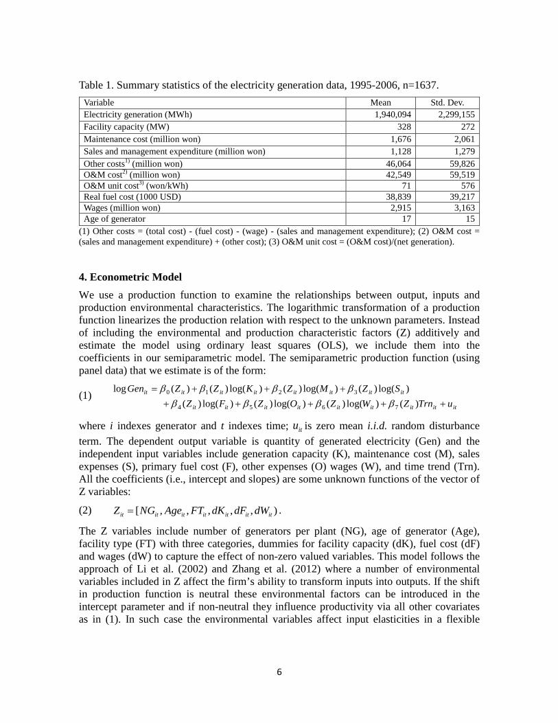
Table 1. Summary statistics of the electricity generation data, 1995-2006, n=1637. Variable Mean Std. Dev. Electricity generation (MWh) 1,940,094 2,299,155 Facility capacity (MW) 328 272 Maintenance cost (million won) 1,676 2,061 Sales and management expenditure (million won) 1,128 1,279 Other costs1) (million won) 46,064 59,826 O&M cost2) (million won) 42,549 59,519 O&M unit cost3) (won/kWh) 71 576 Real fuel cost (1000 USD) 38,839 39,217 Wages (million won) 2,915 3,163 Age of generator 17 15

(1) Other costs = (total cost) - (fuel cost) - (wage) - (sales and management expenditure); (2) O&M cost = (sales and management expenditure) + (other cost); (3) O&M unit cost = (O&M cost)/(net generation).

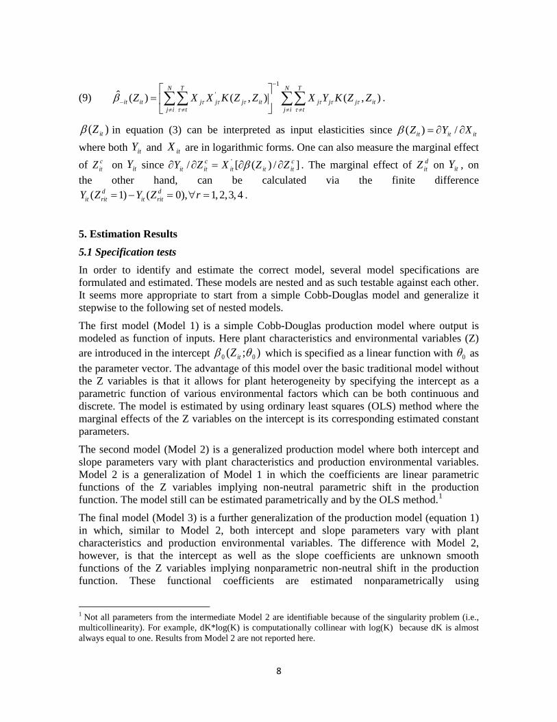
4. Econometric Model We use a production function to examine the relationships between output, inputs and production environmental characteristics. The logarithmic transformation of a production function linearizes the production relation with respect to the unknown parameters. Instead of including the environmental and production characteristic factors (Z) additively and estimate the model using ordinary least squares (OLS), we include them into the coefficients in our semiparametric model. The semiparametric production function (using panel data) that we estimate is of the form:

(1) ititititititititit

itititititititit

uTrnZWZOZFZSZMZKZZGen

++++++++=

)()log()()log()()log()()log()()log()()log()()(log

7654

3210

ββββββββ

where i indexes generator and t indexes time; itu is zero mean i.i.d. random disturbance term. The dependent output variable is quantity of generated electricity (Gen) and the independent input variables include generation capacity (K), maintenance cost (M), sales expenses (S), primary fuel cost (F), other expenses (O) wages (W), and time trend (Trn). All the coefficients (i.e., intercept and slopes) are some unknown functions of the vector of Z variables:

(2) [ , , , , , )it it it it it it itZ NG Age FT dK dF dW= .

The Z variables include number of generators per plant (NG), age of generator (Age), facility type (FT) with three categories, dummies for facility capacity (dK), fuel cost (dF) and wages (dW) to capture the effect of non-zero valued variables. This model follows the approach of Li et al. (2002) and Zhang et al. (2012) where a number of environmental variables included in Z affect the firm’s ability to transform inputs into outputs. If the shift in production function is neutral these environmental factors can be introduced in the intercept parameter and if non-neutral they influence productivity via all other covariates as in (1). In such case the environmental variables affect input elasticities in a flexible

7

manner. For a given level of environmental factor, the model is reduced to the standard constant coefficient Cobb-Douglas production model.

The generalized production model in (1) can be written more compactly as:

(3) itititit uZXY += )(' β

where log( ), [1 log( ), log( ), log( ), log( ), log( ), log( ), ],it it it it it it it it it itY Gen X K M S F O W Trn= = ， and '

0 1 7( ) [ ( ), ( ),..., ( )]it it it itZ Z Z Zβ β β β= . Following Li et al. (2002), the semiparametric estimator of the functional coefficients can be written as:

(4) ∑∑∑∑= =

−

= =

=

N

j

T

itjjj

N

j

T

itjjjit ZZKYXZZKXXZ1 1

1

1 1

' ),(),()(ˆτ

ττττ

τττβ ,

where N and T denotes the number of cross-sections and time periods, respectively, K(.) is a generalized kernel function (Racine and Li, 2004). Here we define ],[ d

itcitit ZZZ = , where

[ , ]cit it itZ NG Age= is a vector containing continuous variables, and

],,,[ ititititdit dWdFdKFTZ = is a vector of categorical and dummy variables. The kernel

function K(.) can then be explicitly written as:

(5) 2 4

1 1

( , ) ( , , )c csj sitc d d d

j it rj rit rs rs

Z ZK Z Z K K Z Z

hτ

τ τ λ= =

−=

∏ ∏ ,

where

(6) 2

1 1(.) exp22

c csj sitc

s

Z ZK

hτ

π

− = −

and

(7) 1 if

(.)/ ( 1) otherwise

d dr rj ritd

r

Z ZK

cτλ

λ

− == −

where, in our application, c, the number of categories, is equal to two, for dummy variables that take the value of 0 or 1. The 1,2sh s∀ = are the bandwidths for each continuous variable in c

itZ , and 1,2,3,4r rλ ∀ = are the bandwidths for each discrete variable in ditZ .

They are selected by minimizing the objective function:

(8) 2'

1 1

ˆ ( )N T

it it it iti t

Y X Zβ−= =

− ∑∑ ,

where

8

(9) 1

'ˆ ( ) ( , ) ( , )N T N T

it it j j j it j j j itj i t j i t

Z X X K Z Z X Y K Z Zτ τ τ τ τ ττ τ

β−

−≠ ≠ ≠ ≠

= ∑∑ ∑∑ .

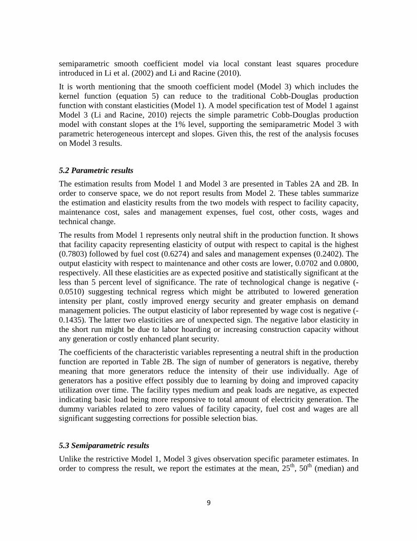
)( itZβ in equation (3) can be interpreted as input elasticities since ( ) /it it itZ Y Xβ = ∂ ∂ where both itY and itX are in logarithmic forms. One can also measure the marginal effect of c

itZ on itY since ]/)([/ ' cititit

citit ZZXZY ∂∂=∂∂ β . The marginal effect of d

itZ on itY , on the other hand, can be calculated via the finite difference

( 1) ( 0), 1, 2,3, 4d dit rit it ritY Z Y Z r= − = ∀ = .

5. Estimation Results 5.1 Specification tests In order to identify and estimate the correct model, several model specifications are formulated and estimated. These models are nested and as such testable against each other. It seems more appropriate to start from a simple Cobb-Douglas model and generalize it stepwise to the following set of nested models.

The first model (Model 1) is a simple Cobb-Douglas production model where output is modeled as function of inputs. Here plant characteristics and environmental variables (Z) are introduced in the intercept );( 00 θβ itZ which is specified as a linear function with 0θ as the parameter vector. The advantage of this model over the basic traditional model without the Z variables is that it allows for plant heterogeneity by specifying the intercept as a parametric function of various environmental factors which can be both continuous and discrete. The model is estimated by using ordinary least squares (OLS) method where the marginal effects of the Z variables on the intercept is its corresponding estimated constant parameters.

The second model (Model 2) is a generalized production model where both intercept and slope parameters vary with plant characteristics and production environmental variables. Model 2 is a generalization of Model 1 in which the coefficients are linear parametric functions of the Z variables implying non-neutral parametric shift in the production function. The model still can be estimated parametrically and by the OLS method.1

The final model (Model 3) is a further generalization of the production model (equation 1) in which, similar to Model 2, both intercept and slope parameters vary with plant characteristics and production environmental variables. The difference with Model 2, however, is that the intercept as well as the slope coefficients are unknown smooth functions of the Z variables implying nonparametric non-neutral shift in the production function. These functional coefficients are estimated nonparametrically using

1 Not all parameters from the intermediate Model 2 are identifiable because of the singularity problem (i.e., multicollinearity). For example, dK*log(K) is computationally collinear with log(K) because dK is almost always equal to one. Results from Model 2 are not reported here.

9

semiparametric smooth coefficient model via local constant least squares procedure introduced in Li et al. (2002) and Li and Racine (2010).

It is worth mentioning that the smooth coefficient model (Model 3) which includes the kernel function (equation 5) can reduce to the traditional Cobb-Douglas production function with constant elasticities (Model 1). A model specification test of Model 1 against Model 3 (Li and Racine, 2010) rejects the simple parametric Cobb-Douglas production model with constant slopes at the 1% level, supporting the semiparametric Model 3 with parametric heterogeneous intercept and slopes. Given this, the rest of the analysis focuses on Model 3 results.

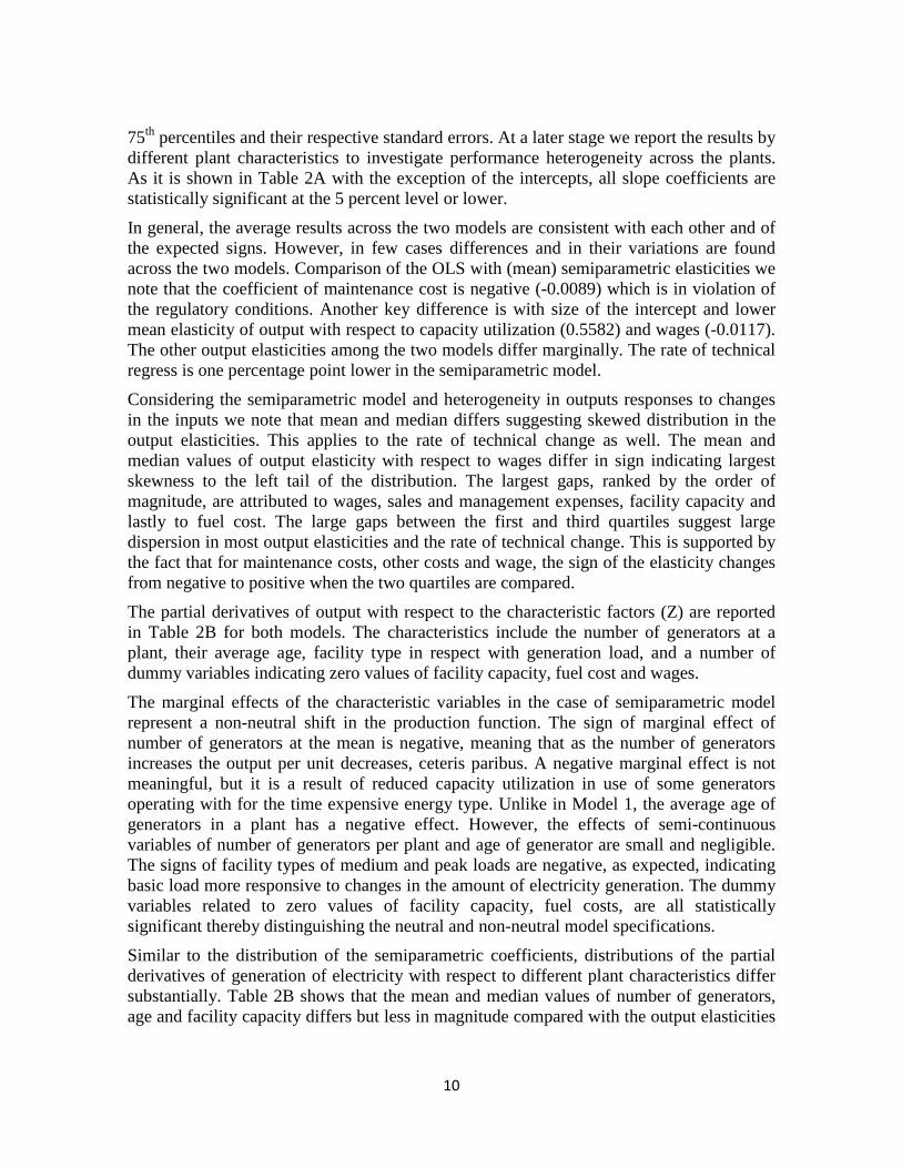
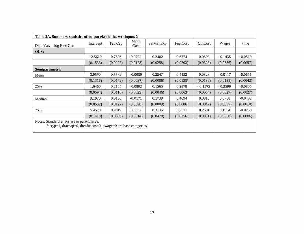
5.2 Parametric results The estimation results from Model 1 and Model 3 are presented in Tables 2A and 2B. In order to conserve space, we do not report results from Model 2. These tables summarize the estimation and elasticity results from the two models with respect to facility capacity, maintenance cost, sales and management expenses, fuel cost, other costs, wages and technical change.

The results from Model 1 represents only neutral shift in the production function. It shows that facility capacity representing elasticity of output with respect to capital is the highest (0.7803) followed by fuel cost (0.6274) and sales and management expenses (0.2402). The output elasticity with respect to maintenance and other costs are lower, 0.0702 and 0.0800, respectively. All these elasticities are as expected positive and statistically significant at the less than 5 percent level of significance. The rate of technological change is negative (-0.0510) suggesting technical regress which might be attributed to lowered generation intensity per plant, costly improved energy security and greater emphasis on demand management policies. The output elasticity of labor represented by wage cost is negative (-0.1435). The latter two elasticities are of unexpected sign. The negative labor elasticity in the short run might be due to labor hoarding or increasing construction capacity without any generation or costly enhanced plant security.

The coefficients of the characteristic variables representing a neutral shift in the production function are reported in Table 2B. The sign of number of generators is negative, thereby meaning that more generators reduce the intensity of their use individually. Age of generators has a positive effect possibly due to learning by doing and improved capacity utilization over time. The facility types medium and peak loads are negative, as expected indicating basic load being more responsive to total amount of electricity generation. The dummy variables related to zero values of facility capacity, fuel cost and wages are all significant suggesting corrections for possible selection bias.

5.3 Semiparametric results Unlike the restrictive Model 1, Model 3 gives observation specific parameter estimates. In order to compress the result, we report the estimates at the mean, 25th, 50th (median) and

10

75th percentiles and their respective standard errors. At a later stage we report the results by different plant characteristics to investigate performance heterogeneity across the plants. As it is shown in Table 2A with the exception of the intercepts, all slope coefficients are statistically significant at the 5 percent level or lower.

In general, the average results across the two models are consistent with each other and of the expected signs. However, in few cases differences and in their variations are found across the two models. Comparison of the OLS with (mean) semiparametric elasticities we note that the coefficient of maintenance cost is negative (-0.0089) which is in violation of the regulatory conditions. Another key difference is with size of the intercept and lower mean elasticity of output with respect to capacity utilization (0.5582) and wages (-0.0117). The other output elasticities among the two models differ marginally. The rate of technical regress is one percentage point lower in the semiparametric model.

Considering the semiparametric model and heterogeneity in outputs responses to changes in the inputs we note that mean and median differs suggesting skewed distribution in the output elasticities. This applies to the rate of technical change as well. The mean and median values of output elasticity with respect to wages differ in sign indicating largest skewness to the left tail of the distribution. The largest gaps, ranked by the order of magnitude, are attributed to wages, sales and management expenses, facility capacity and lastly to fuel cost. The large gaps between the first and third quartiles suggest large dispersion in most output elasticities and the rate of technical change. This is supported by the fact that for maintenance costs, other costs and wage, the sign of the elasticity changes from negative to positive when the two quartiles are compared.

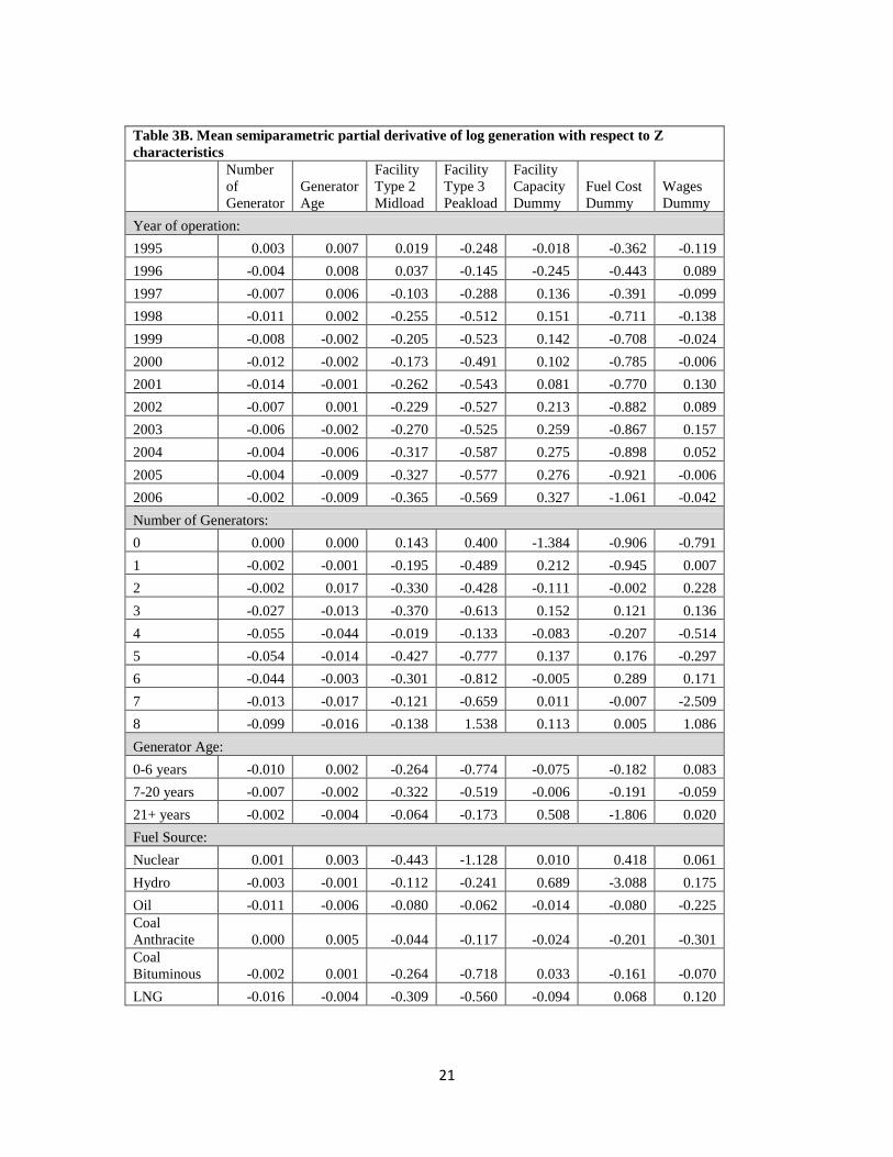
The partial derivatives of output with respect to the characteristic factors (Z) are reported in Table 2B for both models. The characteristics include the number of generators at a plant, their average age, facility type in respect with generation load, and a number of dummy variables indicating zero values of facility capacity, fuel cost and wages.

The marginal effects of the characteristic variables in the case of semiparametric model represent a non-neutral shift in the production function. The sign of marginal effect of number of generators at the mean is negative, meaning that as the number of generators increases the output per unit decreases, ceteris paribus. A negative marginal effect is not meaningful, but it is a result of reduced capacity utilization in use of some generators operating with for the time expensive energy type. Unlike in Model 1, the average age of generators in a plant has a negative effect. However, the effects of semi-continuous variables of number of generators per plant and age of generator are small and negligible. The signs of facility types of medium and peak loads are negative, as expected, indicating basic load more responsive to changes in the amount of electricity generation. The dummy variables related to zero values of facility capacity, fuel costs, are all statistically significant thereby distinguishing the neutral and non-neutral model specifications.

Similar to the distribution of the semiparametric coefficients, distributions of the partial derivatives of generation of electricity with respect to different plant characteristics differ substantially. Table 2B shows that the mean and median values of number of generators, age and facility capacity differs but less in magnitude compared with the output elasticities

11

and compared with the zero characteristics dummy variables. The largest difference is attributed to dummy variables related to zero facility capacity and fuel costs. The gaps between the 1st and 3rd quartiles are much larger suggesting skewed distribution of these non-neutral shifters of production. Facility load type is the main shifter followed by fuel cost and wages.

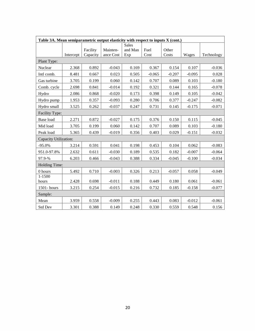
5.4 Heterogeneity by plant characteristics Similar to the large variations in the observation specific levels of output elasticities and partial effects of characteristics on production, there are also large variations in their averages across different generator characteristics and over time. The characteristics of interest include: number of generators per plant, average age of generator in years, fuel source, plant type, facility load type, percentage facility utilization rate, and holding time measured in hours per year. These are reported in Table 3A and 3B. In order to conserve spaces, the point elasticity and marginal effects are not reported here.

A close look at the changes in the mean output elasticities of inputs over time (Table 3A) show that the output elasticity with respect to facility capacity (which is the largest) is declining over time, while the output elasticity in respect with fuel cost is increasing. The third largest output elasticity is that of sales and management expenditure which is declining. All of these three key output elasticities are positive in each year. Similar to these three cases where we find trends in their development over time, -- there is positive trend in the maintenance and other costs which switch from negative to positive in 2005/6 and 1997/8 respectively. The output elasticity of wages is small and mainly negative and without any trend in its development. The high yearly rate of technical regress ranges from 7.8 percent to 4.9 percent.

The partial effect with respect to fuel cost dummy is large, negative and declining over time. Similar negatively signed and trended partial effects are observed in relation with facility types of medium and peak loads compared with the base load which serves as reference load type. Marginal effect of facility capacity is relatively large and changed from negative to positive over time. The marginal wage effect is low and its mean value is volatile over time. The marginal effects of age and number of generator effect are small (see Table 3B).

The output elasticities of facility capacity, sales and management costs are negatively related to the number of generators, while fuel cost is positively related due to the fact that peak load generators are operating with high cost of primary fuel sources. There is also a positive relationship between output elasticity of wages and number of generators suggesting that wages at the peak load generators operating at the margin capacity is higher. The rate of technical regress in general increases with the number of generators per plant. Variations in the marginal effects of output with respect to generator characteristics are less systematic in relation to the number of generators per plant (see Tables 3A and 3B).

12

The difference in the output elasticities across age cohort of generators is pronounced. The elasticity of output with respect to facility capacity is negatively correlated to the age of generator. Similar is the case with fuel cost, and wages, while it is positively correlated with maintenance cost and sales and management expenditures. Similar relationships are found between age and the marginal effects of generator characteristics. The number of generators, facility capacity, higher loads and facility dummy variable are all positively related, while age of generator and fuel cost dummy variables are negatively related.

The output elasticity of facility capacity is highest for nuclear, the two types of coals and hydro plants, while it is lowest for oil and gas driven plants which are used only as peak load. The sales and management expenditures is highest for hydro and gas plants. The fuel cost is the highest for gas and oil but lowest for hydro plants. The other cost elasticity with the exception of hydro which is surprisingly negative is almost of equal size. Oil and gas due to their high price level and their volatility contribute most to the technical regress. Considering the marginal effects, again hydro, oil and gas fuel driven generators are more responsive than those generators driven by nuclear and coal sources.

In the case of plant type, nuclear, combined cycle, hydro pump and internal combustion show the highest output elasticities with respect to facility capacity. The lowest output elasticity is related to gas turbine and small hydro type. In terms of fuel cost, the output elasticity is found to be high for gas turbine, hydro pump and small hydro, while it is low for combined cycle and negative for internal combustion. Internal combustion is the only plant type which shows technical progress, while remaining types are subject to technical regress, which the rate is highest for gas turbine type. Again we find large variations in the marginal effects across plant types. The main variations are attributed to load type and facility capacity and fuel cost dummy variable.

As expected the base load facility capacity has higher output elasticity, followed by the peak load and it is lowest for the middle load capacity. The low responsiveness for middle load capacity suggests that volatility in electricity demand is high which is mainly satisfied by the base and peak loads. The costs attributed to sale, management and fuel show large variations across different load capacities. It is as expected highest for the peak load. The output elasticity with respect to wages reflecting efficiency in use of labor at these plant types differs. It is negative for the peak load plants. The rate of technical regress is lowest for the middle load which is it capacity is utilized less. Similar results are found for the partial effects in the case of middle load.

We note a clear difference between output elasticity of facility capacity and its rate of utilization. In particular the rate of technical regress is much higher for the plants with low rate of capacity utilization. We note lower differences in outputs responsiveness to changes in costs of fuel and sales and management expenditure. Again variation in the marginal effects is large in respect with degree of capacity utilization of generators/plants.

The last plant characteristic as source of heterogeneity is the generators holding time for repairs, services and malfunctions. We note the output elasticities with respect to the key factor of facility capacity and sales and management expenditure are inversely related to the holding time. A high maintenance cost affects the rate of holding time negatively. The

13

rate of technical regress is much higher for the plants classified in the category with high holding times. Significant heterogeneity in the size of partial effects is also observed in respect with holding time of generators/plants operation.

5.5 Policy implications of the results Unlike traditional models where supply response is practiced, in the deregulated electricity markets case demand response and its management is increasingly employed (Heshmati, 2013a). In situations with expansion of demand for electricity, it might be cheaper to reduce demand than to increase supply. This is evidenced in particular in cases where price is regulated below the cost of incremental supply which does not give incentives to consumers to conserve. In such cases, it is better for the utility to pay price corrections in exchange for consumer demand reductions to balance supply and demand. The collapse of oil prices in 1998-1999 led to increased capacity expansion and the following energy price surge led to excess capacity which further increased its cost coverage. These differences between supply and demand response and increased marginal cost for incremental supply explain the rate of technical regress in our results.

In line with the result here, several previously conducted studies (Heshmati, 2013b) show evidence of a decreasing trend in the performance in the electricity market. After separation in 2001 the DEA based efficiency is reduced slightly due to a lower scale efficiency change. The results show that, the efficiency of generating companies did not improve, as was expected, after the separation process. However, the magnitude of scale effect was increased after the separation. The MPI results suggest decreased efficiency over the period. By separating the period into before and after separation, one can see a slowly increasing pattern before 2001 while a gradually decreasing trend after 2001. Inefficiency comes from scale efficiency in the before-restructuring time, while in the after-restructuring time it comes from decline in the technical change. This means there were not enough technological improvements in the electricity generation industry after 2001. In total, productivity declined over time which is consistent with our findings of technical regress.

Heshmati (2012) analyzes the technical efficiency of generation units, rank each unit for comparative assessment of their technical efficiency status and suggests policy recommendations. Although most of strategic activities for generation are decided by company or business unit levels, one can suggest suitable performance enhancement strategies and measures at the generator level. Based on the efficiency result, the effect from facility age or technological change was found to be small. Inefficiency of units is mostly related to the type of facility. It means that the market operating scheme is a basic factor in the operation performance. Although the facility type affects generation as the most important factor, in the view of control, the flexible labor management can be recognized as an easier way to introduce changes. More flexibility in human resource management in form of the labor transfer and labor pool of the same generation source or the same generation type facilities has been suggested. However, such reallocation of labor among generation companies is not an easy task in reality. The inflexible labor use in the

14

generation may explain the low output elasticity of labor and for some segments irregularities in the labor coefficient.

The strategy for improving the effectiveness of the fuel factor is most urgent. The increased fuel price is very likely the most important factor attributed to productivity decrease. Thus, a stabilizing strategy in response to the volatile fuel price in the long term is required. That is, not only a low purchasing price but also a stabilization of fuel price is important measures to reduce variations in the efficiency and productivity levels. In this regard, the long term fuel purchasing and purchasing diversification should be considered. A reorganization of the electricity generation sector by the same fuel type can be a way to obtain high purchasing power. It can have fuel purchasing power under the unified simple energy source and also make the operational performance higher and organizational management easier.

6. Summary and Conclusion Semiparametric varying-coefficient method used in the paper accommodates both qualitative and quantitative covariates in specification of the varying coefficients. In this paper we used the semiparametric approach to analyze the impact of load factor, facility and generator type and other characteristics on the productivity of Korean electric power plants. The model captures important heterogeneities in the effect arising from public energy policy across power plants and over time. Various specification tests are conducted to compare the model performance.

The tradition parametric models such as the Cobb-Douglas can be derived as a special case of the smooth coefficient model with constant elasticities. A model specification test rejects the simple parametric production model with constant slopes, supporting the semiparametric model with heterogeneous intercept and slopes. Using a unique generator level panel dataset, we find that the impact of load factor and generator and facility types on power generation varies substantially. The period of our study 1995-2006, which covers the electricity generation market restructuring period of 2001, allows us to examine the impact of reform on the performance of plants. The variations in the impact are large across different plant characteristics. This result is useful for the public energy policy in Korea.

The elasticity estimates from the two models with respect to facility capacity, fuel cost, wages, other inputs costs and technical change are provided. In general, the output elasticity results across the two models are consistent with each other, have expected signs and statistical significance. The results from simple and varying coefficient semiparametric models represent neutral and non-neutral shifts in the production function, respectively. The rate of technological change is negative suggesting technical regress which might be attributed to lowered generation intensity per unit, improved energy security and practice of demand management policies in the electricity market. The output elasticity of labor represented by wage cost is unexpectedly negative which might be due to labor hoarding, faster wage increases than labor productivity, increasing construction capacity and enhanced power plant security. The estimated effects of plant characteristics are as

15

expected where increased number of generator reduce the intensity in their use individually. Age of generators has a positive effect indicating learning by doing over time. The facility types show that basic load being more responsive to total generation.

The smooth coefficient model gives rise to observation specific coefficient estimates. Summary of the result at different segments of the distribution suggest presence of heterogeneity in estimates by various plants characteristics. Large skewness in the distributions of output elasticities is also observed. The largest gaps are attributed to wages, sales and management expenses, facility capacity and fuel cost. The large gaps between the first and third quartiles also suggest large dispersion in most output elasticities and the rate of technical change. A comparison of the OLS elasticiticities with the mean semiparametric elasticities led to a number of differences, mainly, related to the output elasticities with respect to capacity utilization and wages. The other mean output elasticities differ marginally, while the rate of technical regress is lower in the semiparametric model. In sum, the results suggest presence of large heterogeneity in the plant’s output response to changes in the production factors and technological change.

Similar to the large variations in the levels of output elasticities and marginal effects of various characteristics on production, there is also large variation in their averages across different generator characteristics and over time. The key factors of interest include: number of generators per plant, average age of generator in years, fuel source, plant type, facility load type, facility utilization rate, and holding time. Focusing at the changes in the mean output elasticities of inputs over time, we note that output elasticity with respect to facility capacity is declining over time, while the output elasticity with respect to fuel cost is increasing.

Large heterogeneity in output elasticities and marginal effects of plant characteristics over time and across different plant characteristics suggest that the volatile fuel price development, the high quasi fixed wage costs, difficulties in investment decision in new capacity considering the specific primary fuel types, as well as capacity distribution and utilization are the key issues to be considered in the strategy for improving the effectiveness of the fuel factor. The increased and volatile fuel price is likely to be the main source of productivity decrease. A reorganization of the electricity generation sector by the same fuel type can be a way to obtain high purchasing power and stability in fuel prices. It can also make the operational performance higher and organizational management easier.

References Choi K.H. and B.W. Ang (2002), Measuring Thermal Efficiency Improvement in Power

Generation: The Divisia Decomposition Approach, Energy 27(5), 447-455.

Fan Y. and Q. Li (1996), Consistent Model Specification Tests: Omitted Variables and Semiparametric Functional Forms, Econometrica 65, 865-890.

Griliches Z. (1979), Issues in Assessing the Contribution of Research and Development to Productivity Growth, Bell Journal of Economics 10, 92-116.

16

Griliches Z. (1986), Productivity, R&D and Basic Research at the Firm Level in the 1970's, American Economic Review 76, 141-154.

Hastie T. and R. Tibshirani (1993), Varying Coefficient Models, Journal of the Royal Statistical Society, Series B, 55, 757-796.

Heshmati A. (2012), Economic Fundamentals of Power Plants Performance, Routledge Studies in the Modern World Economy #97, Routledge.

Heshmati A. (2013a), Demand, Customer Base-Line and Demand Response in the Electricity Market: A Survey, Journal of Economics Surveys, forthcoming.

Heshmati A. (2013b), Efficiency and Productivity Impacts of Restructuring the Korean Electricity Generation, Korea and the World Economy 14(1), 000-000.

Lee B.H. and H.H. Ahn (2006), Electricity Industry Restructuring Revisited: The Case of Korea, Energy Policy 34(10), 1115-1126.

Li Q., C. Huang, D. Li and T. Fu (2002), Semiparametric Smooth Coefficient Models, Journal of Business Economics and Statistics 20, 412-422.

Li Q. and J. Racine (2007), Nonparametric Econometrics: Theory and Practice, Princeton University Press, Princeton.

Li Q. and J. Racine (2010), Smooth Varying-Coefficient Estimation and Inference for Qualitative and Quantitative Data, Econometric Theory 26, 1607-1637.

Park S.U. and J.B. Lesourd (2000), The Efficiency of Conventional Fuel Power Plants in South Korea: A Comparison of Parametric and Non-Parametric Approaches, International Journal of Production Economics 63(1), 59-67.

Racine J. and Q. Li (2004), Nonparametric Estimation of Regression Functions with both Categorical and Continuous Data, Journal of Econometrics 119, 99-130.

Robinson P.M. (1988), Root-N-Consistent Semiparametric Regression, Econometrica 56, 931-954.

Stock J.H. (1989), Nonparametric Policy Analysis, Journal of the American Statistical Association 84, 567-575.

Zhang R., K. Sun, M.S. Delgado and S.C. Kumbhakar (2012), Productivity in China’s High Technology Industry; Regional Heterogeneity and R&D, Technological Forecasting and Social Change 79, 127-141.

17

Table 2A. Summary statistics of output elasticities wrt inputs X

Dep. Var. = log Elec Gen Intercept Fac Cap Main. Cost SalManExp FuelCost OthCost Wages time

OLS:

12.5610 0.7803 0.0702 0.2402 0.6274 0.0800 -0.1435 -0.0510

(0.1536) (0.0297) (0.0173) (0.0258) (0.0203) (0.0326) (0.0386) (0.0057)

Semiparametric:

Mean 3.9590 0.5582 -0.0089 0.2547 0.4432 0.0828 -0.0117 -0.0611

(0.1316) (0.0172) (0.0037) (0.0086) (0.0138) (0.0139) (0.0138) (0.0042) 25% 1.6460 0.2165 -0.0802 0.1565 0.2578 -0.1575 -0.2599 -0.0805

(0.0594) (0.0110) (0.0029) (0.0046) (0.0063) (0.0064) (0.0027) (0.0027)

Median 3.1970 0.6186 -0.0171 0.1739 0.4694 0.0810 0.0768 -0.0432

(0.0532) (0.0127) (0.0020) (0.0009) (0.0086) (0.0047) (0.0037) (0.0010) 75% 5.4570 0.9019 0.0332 0.3135 0.7571 0.2501 0.1354 -0.0253

(0.1419) (0.0359) (0.0014) (0.0470) (0.0256) (0.0031) (0.0050) (0.0006) Notes: Standard errors are in parentheses. factyp=1, dfaccap=0, dreafuecos=0, dwage=0 are base categories.

18

Table 2B. Summary statistics of partial derivatives of log electricity generation with respect to Characteristics Z Dep. Var. = log Elec Gen No Gen Age FacType 2 FacType 3 DFacCap DFuelCost Dwages

OLS:

-0.1710 0.0056 -0.3274 -0.7786 -3.9403 -6.3124 -0.2423

(0.0210) (0.0018) (0.0662) (0.0626) (0.1845) (0.1950) (0.2486)

Semiparametric:

Mean -0.0064 -0.0013 -0.2151 -0.4726 0.1531 -0.7526 0.0100

(0.0008) (0.0006) (0.0136) (0.0195) (0.0362) (0.0572) (0.0275) 25% -0.0033 -0.0101 -0.4261 -0.8777 -0.0002 -0.5766 -0.2546

(0.0001) (0.0003) (0.0142) (0.0315) (0.0017) (0.0174) (0.0100)

Median 0.0000 0.0003 -0.1817 -0.4307 0.0000 -0.0112 -0.0240

(0.0000) (0.0002) (0.0096) (0.0113) (0.0000) (0.0017) (0.0069) 75% 0.0001 0.0106 0.0000 -0.0145 0.0083 0.3014 0.2182

(0.0001) (0.0004) (0.0066) (0.0101) (0.0009) (0.0177) (0.0061) Notes: Standard errors are in parentheses. factyp=1, dfaccap=0, dreafuecos=0, dwage=0 are base categories.

19

Table 3A. Mean semiparametric output elasticity with respect to inputs X

Intercept

Facility Capacity

Mainten- ance Cost

Sales and Man Exp

Fuel Cost

Other Costs Wages Technology

Year of operation: 1995 4.989 0.612 -0.036 0.362 0.371 -0.019 -0.009 -0.067 1996 5.246 0.566 -0.056 0.364 0.363 -0.011 0.005 -0.078 1997 4.306 0.591 -0.022 0.283 0.431 -0.005 0.053 -0.075 1998 4.258 0.579 -0.016 0.284 0.433 -0.030 0.091 -0.076 1999 3.934 0.579 -0.009 0.270 0.436 0.092 -0.039 -0.052 2000 3.822 0.565 -0.006 0.257 0.445 0.094 -0.019 -0.054 2001 3.799 0.560 -0.003 0.248 0.453 0.080 0.002 -0.058 2002 3.591 0.540 -0.003 0.213 0.467 0.152 -0.047 -0.060 2003 3.705 0.534 -0.001 0.215 0.468 0.130 -0.032 -0.064 2004 3.488 0.541 0.008 0.207 0.468 0.143 -0.043 -0.049 2005 3.516 0.533 0.009 0.208 0.467 0.148 -0.044 -0.052 2006 3.446 0.523 0.009 0.204 0.478 0.152 -0.037 -0.056 Number of Generators: 0 9.394 0.478 -0.152 0.636 0.347 -0.238 0.021 -0.300 1 3.736 0.614 0.000 0.253 0.375 0.149 -0.047 -0.038 2 3.578 0.337 -0.049 0.285 0.692 -0.052 0.035 -0.072 3 3.528 0.392 -0.032 0.217 0.770 -0.161 0.074 -0.066 4 5.480 0.353 0.041 0.428 0.603 -0.082 -0.139 -0.081 5 6.398 0.197 -0.046 0.238 0.735 -0.509 0.460 -0.234 6 5.068 0.278 -0.081 0.207 0.779 -0.063 -0.130 -0.058 7 16.079 -0.100 0.017 -0.858 0.695 -0.787 1.834 -1.491 8 14.903 0.109 -0.023 -0.186 1.005 -0.839 1.485 -1.329 Generator Age: 0-6 years 2.124 0.632 -0.019 0.219 0.585 0.047 0.085 -0.062 7-20 years 3.871 0.574 -0.052 0.243 0.470 0.104 0.052 -0.090 21+ years 5.587 0.481 0.044 0.296 0.297 0.091 -0.158 -0.030 Fuel Source: Nuclear 2.368 0.892 -0.043 0.169 0.367 0.154 0.107 -0.036 Hydro 7.027 0.598 -0.003 0.455 0.107 -0.077 -0.129 0.004 Oil 3.705 0.199 0.060 0.142 0.707 0.089 0.103 -0.180 Coal Anthracite 2.698 0.841 -0.014 0.192 0.321 0.144 0.165 -0.078 Coal Bituminous 2.086 0.868 -0.020 0.173 0.398 0.149 0.105 -0.042 LNG 3.525 0.262 -0.037 0.247 0.731 0.145 -0.175 -0.071

20

Table 3A. Mean semiparametric output elasticity with respect to inputs X (cont.)

Intercept

Facility Capacity

Mainten- ance Cost

Sales and Man Exp

Fuel Cost

Other Costs Wages Technology

Plant Type: Nuclear 2.368 0.892 -0.043 0.169 0.367 0.154 0.107 -0.036 Intl comb. 8.481 0.667 0.023 0.505 -0.065 -0.207 -0.095 0.028 Gas turbine 3.705 0.199 0.060 0.142 0.707 0.089 0.103 -0.180 Comb. cycle 2.698 0.841 -0.014 0.192 0.321 0.144 0.165 -0.078 Hydro 2.086 0.868 -0.020 0.173 0.398 0.149 0.105 -0.042 Hydro pump 1.953 0.357 -0.093 0.280 0.706 0.377 -0.247 -0.082 Hydro small 3.525 0.262 -0.037 0.247 0.731 0.145 -0.175 -0.071 Facility Type: Base load 2.271 0.872 -0.027 0.175 0.376 0.150 0.115 -0.045 Mid load 3.705 0.199 0.060 0.142 0.707 0.089 0.103 -0.180 Peak load 5.365 0.439 -0.019 0.356 0.403 0.029 -0.151 -0.032 Capacity Utilization: -95.0% 3.214 0.591 0.041 0.198 0.453 0.104 0.062 -0.083 951.0-97.8% 2.632 0.611 -0.030 0.189 0.535 0.182 -0.007 -0.064 97.9-% 6.203 0.466 -0.043 0.388 0.334 -0.045 -0.100 -0.034 Holding Time: 0 hours 5.492 0.710 -0.003 0.326 0.213 -0.057 0.058 -0.049 1-1500 hours 2.428 0.698 -0.011 0.188 0.449 0.180 0.061 -0.061 1501- hours 3.215 0.254 -0.015 0.216 0.732 0.185 -0.158 -0.077 Sample: Mean 3.959 0.558 -0.009 0.255 0.443 0.083 -0.012 -0.061 Std Dev 3.301 0.388 0.149 0.248 0.330 0.559 0.548 0.156

21

Table 3B. Mean semiparametric partial derivative of log generation with respect to Z characteristics

Number of Generator

Generator Age

Facility Type 2 Midload

Facility Type 3 Peakload

Facility Capacity Dummy

Fuel Cost Dummy

Wages Dummy

Year of operation: 1995 0.003 0.007 0.019 -0.248 -0.018 -0.362 -0.119 1996 -0.004 0.008 0.037 -0.145 -0.245 -0.443 0.089 1997 -0.007 0.006 -0.103 -0.288 0.136 -0.391 -0.099 1998 -0.011 0.002 -0.255 -0.512 0.151 -0.711 -0.138 1999 -0.008 -0.002 -0.205 -0.523 0.142 -0.708 -0.024 2000 -0.012 -0.002 -0.173 -0.491 0.102 -0.785 -0.006 2001 -0.014 -0.001 -0.262 -0.543 0.081 -0.770 0.130 2002 -0.007 0.001 -0.229 -0.527 0.213 -0.882 0.089 2003 -0.006 -0.002 -0.270 -0.525 0.259 -0.867 0.157 2004 -0.004 -0.006 -0.317 -0.587 0.275 -0.898 0.052 2005 -0.004 -0.009 -0.327 -0.577 0.276 -0.921 -0.006 2006 -0.002 -0.009 -0.365 -0.569 0.327 -1.061 -0.042 Number of Generators: 0 0.000 0.000 0.143 0.400 -1.384 -0.906 -0.791 1 -0.002 -0.001 -0.195 -0.489 0.212 -0.945 0.007 2 -0.002 0.017 -0.330 -0.428 -0.111 -0.002 0.228 3 -0.027 -0.013 -0.370 -0.613 0.152 0.121 0.136 4 -0.055 -0.044 -0.019 -0.133 -0.083 -0.207 -0.514 5 -0.054 -0.014 -0.427 -0.777 0.137 0.176 -0.297 6 -0.044 -0.003 -0.301 -0.812 -0.005 0.289 0.171 7 -0.013 -0.017 -0.121 -0.659 0.011 -0.007 -2.509 8 -0.099 -0.016 -0.138 1.538 0.113 0.005 1.086 Generator Age: 0-6 years -0.010 0.002 -0.264 -0.774 -0.075 -0.182 0.083 7-20 years -0.007 -0.002 -0.322 -0.519 -0.006 -0.191 -0.059 21+ years -0.002 -0.004 -0.064 -0.173 0.508 -1.806 0.020 Fuel Source: Nuclear 0.001 0.003 -0.443 -1.128 0.010 0.418 0.061 Hydro -0.003 -0.001 -0.112 -0.241 0.689 -3.088 0.175 Oil -0.011 -0.006 -0.080 -0.062 -0.014 -0.080 -0.225 Coal Anthracite 0.000 0.005 -0.044 -0.117 -0.024 -0.201 -0.301 Coal Bituminous -0.002 0.001 -0.264 -0.718 0.033 -0.161 -0.070 LNG -0.016 -0.004 -0.309 -0.560 -0.094 0.068 0.120

22

Table 3B. Mean semiparametric partial derivative of log generation with respect to Z characteristics (cont.)

Number of Generator

Generator Age

Facility Type 2 Midload

Facility Type 3 Peakload

Facility Capacity Dummy

Fuel Cost Dummy

Wages Dummy

Plant Type: Nuclear 0.001 0.003 -0.443 -1.128 0.010 0.418 0.061 Intl comb. 0.000 -0.001 0.162 -0.012 0.905 -3.577 0.239 Gas turbine -0.011 -0.006 -0.080 -0.062 -0.014 -0.080 -0.225 Comb. cycle 0.000 0.005 -0.044 -0.117 -0.024 -0.201 -0.301 Hydro -0.002 0.001 -0.264 -0.718 0.033 -0.161 -0.070 Hydro pump -0.011 -0.004 -1.067 -1.042 -0.066 -1.380 -0.049 Hydro small -0.016 -0.004 -0.309 -0.560 -0.094 0.068 0.120 Facility Type: Base load -0.001 0.002 -0.288 -0.758 0.017 0.020 -0.063 Mid load -0.011 -0.006 -0.080 -0.062 -0.014 -0.080 -0.225 Peak load -0.009 -0.002 -0.205 -0.393 0.317 -1.590 0.149 Capacity Utilization: -95.0% -0.004 -0.003 -0.139 -0.463 0.072 -0.223 0.131 951.0-97.8% -0.007 0.002 -0.279 -0.667 -0.105 0.093 -0.049 97.9-% -0.008 -0.002 -0.233 -0.277 0.517 -2.244 -0.064 Holding Time: 0 hours -0.002 0.001 -0.126 -0.462 0.432 -1.648 0.087 1-1500 hours -0.004 0.002 -0.146 -0.419 0.012 0.010 -0.195 1501- hours -0.014 -0.006 -0.384 -0.528 -0.091 -0.214 0.075 Sample: Mean -0.006 -0.001 -0.215 -0.473 0.153 -0.753 0.010 Std Dev 0.031 0.026 0.534 0.637 1.451 2.198 1.110