Estimation of Thermal and Hydraulic Characteristics of Compact Brazed Plate Heat Exchangers Vijaya Sekhar Gullapalli Doctoral Thesis

Division of Heat Transfer

Department of Energy Sciences

Faculty of Engineering, LTH

Lund University

P.O. Box 118

SE-221 00 Lund

Sweden

Estimation of Thermal and Hydraulic Characteristics of Compact Brazed

Plate Heat Exchangers

Vijaya Sekhar Gullapalli

Department of Energy Sciences Faculty of Engineering

Heat Transfer Research SWEP International AB P. O. Box 105 SE-561 22 Landskrona Sweden Department of Heat Transfer Department of Energy Sciences Faculty of Engineering Lund University Box 118 SE-221 00 Lund Sweden Doctoral Thesis in Heat Transfer ©Vijaya Sekhar Gullapalli, SWEP International AB Lund 2013

i

Abstract This thesis work presents various performance estimation methods of compact brazed plate heat exchangers (BPHE) operating in single phase, condenser, evaporator, cascaded and transcritical applications. Such methods play a vital role in development of heat exchanger selection software and during geometry parameter estimation in the new product development process.

The suitability of employing commercial computational fluid dynamics (CFD) codes for estimating single phase thermal and hydraulic performance is investigated. Parametric studies are conducted on geometries of single phase fluid sections to isolate and quantify the influence of individual geometric parameters. The influence of mesh characteristics, choice of boundary conditions and turbulent flow modeling on the accuracy of the thermal and hydraulic predictions is presented. Benefits of simulation of fluid flow in entire channels and characteristics of channel flow for different geometric patterns are also presented.

A computationally light, general, robust and continuous rating calculation method is developed for implementation in BPHE selection software. The pressure-enthalpy based method provides a generic rating core for various types of applications and provides extensive post processing information of the heat transfer process. General single phase thermal and hydraulic empirical correlations are developed as functions of plate geometric parameters. For facilitating better integration of the developed calculation method with other refrigeration system simulation software, first or higher order continuity is maintained in the sub-routines used for calculating local heat transfer coefficients and refrigerant properties. A new finite grid interpolation method is developed for fast and accurate retrieval of refrigerant properties. The developed method is currently implemented in SSPG7 (BPHE selection software of SWEP International AB) for supporting transcritical CO2 calculations and cascaded heat exchanger calculations.

Additionally, the methods developed for single phase and two phase test data evaluation based on meta-heuristic optimization routines is also presented. The application and results of using the developed rating models for various types of calculations is summarized. Other topics such as influence of variable fluid properties on BPHE rating calculations, influence of multi-pass flow arrangement on lumped BPHE rating calculations are briefly presented.

ii

To My Parents

Shri. Abbulu Chowdary Gullapalli

Smt. Ramadevi Gullapalli

iii

Acknowledgements I would like to express my sincere gratitude to all people, who, in all ways, have assisted and inspired me during the course of my research. First, I extend my sincere gratitude to the management of SWEP International AB, Landskrona, for providing me the privilege to conduct the industrial doctoral research at Lund Technical University. I express my gratitude to my supervisor, Prof. Bengt Sundén, for his valuable help during discussions on several ideas, thesis formulation and publication review. I thank him for his patience and understanding of the limitations while conducting industrial doctoral research. I also thank Prof. Jinliang Yuan, Lund University and Dr. Dirk Sterner, SWEP International AB for their support during this work. I extend my sincere thanks to Christel Elmqvist-Möller, Manager, Heat Transfer Research, for the drive, opportunity and inspiration during the work. I also thank all the members, past and present, at the departments of Heat Transfer Research, Innovation, Software Architecture, Design, Application Management, Sales and Marketing at SWEP International AB for the valuable discussions during the course of this work. I also thank all the members, past and present, at the departments of Heat Transfer Research and Software Group at SWEP India Innovation Center, Bangalore, for their direct and indirect contributions during this work. Further, I wish to thank all the authors whom I have referred in this work, whose work provided better insight into heat transfer theory and inspired new ideas in modeling of plate heat exchangers. I especially thank, Tomas Dahlberg and Sven Andersson at Innovation, SWEP International AB, for valuable discussions on heat exchanger design and for providing geometries for CFD simulations; Patrik Eriksson and Mats Jönsson at Heat Transfer Research, SWEP International AB, for providing insight into heat exchanger testing methods for several applications; Arpita Maji and team members at SWEP IIC, Bangalore, for support during the software development tasks. I am very thankful to my parents and my family, for their support during this work. I particularly thank my uncle, Mr. Venkata Subbarao Karuturi, and my brother, Mr. Raja Sekhar Gullapalli, for all the love and inspiration during this work. I offer my heartfelt thanks to my beloved wife, Aravinda Gajjarapu, for all the love, patience and sacrifices during the course of this work. This work would not have been possible without your care and concern. Keywords: Brazed plate heat exchangers, heat exchanger selection software, CFD, heat transfer, pressure drop, discretized calculations, transcritical-CO2 calculations, heat exchanger rating, evaporation, condensation, refrigerant properties

iv

List of Publications The main body of the thesis work is based on the following publications: A. Gullapalli, V.S., Sundén, B., 2013. “CFD simulation of heat transfer and pressure drop in

compact brazed plate heat exchangers”, Submitted for publication to the Journal of Heat Transfer Engineering on June 7th 2012, Conditional acceptance received on February 28th, 2013. Full paper submission due on May 15th, 2013

B. Gullapalli, V.S., 2011. “Design of high efficiency compact brazed plate heat exchangers using CFD”, The 23rd IIR International Congress of Refrigeration, Prague, Paper ID: 614

C. Gullapalli, V.S., Sundén, B., 2011. “Generalized performance analysis of compact brazed plate heat exchangers”, Proceedings of the 21st national and 10th ISHMT-ASME heat and mass transfer conference, December 27-30, IIT Madras, India.

D. Gullapalli, V.S., Sundén, B., 2011. “Condensation and evaporation in compact brazed plate heat exchangers: Generalized rating method”, Proceedings of the 21st national and 10th ISHMT-ASME heat and mass transfer conference, December 27-30, IIT Madras, India.

E. Gullapalli, V.S., 2007. “Condensation in compact brazed plate heat exchangers:

Evaluation and performance analysis”, Heat transfer in components and systems for sustainable energy technologies, 18-20 April 2007, Chambery, France.

Some sections of the current work are extensions of the earlier work done for the degree of licentiate in engineering. Gullapalli, V.S., 2008. “On Performance Analysis of Plate Heat Exchangers”, Thesis for the degree of licentiate in engineering, ISRN LUTMDN/TMHP—08/7055—SE, ISSN 0282-1990, Division of Heat Transfer, Department of Energy Sciences, Faculty of Engineering, LTH, Lund University, Sweden.

v

Symbols A Area m² C Chisholm correlation empirical constant [-]

pC Specific heat capacity at constant pressure J/ (kg K)

hD Hydraulic diameter m

e Entrainment factor [-] e Specific internal energy J/ kg f Friction factor [-] F Two-phase pressure drop multiplier [-] F Convective boiling enhancement factor [-] g Acceleration due to gravity m/sec² G Mass velocity kg/ (m² sec) h Convective heat transfer coefficient W/ (m² K) i Specific enthalpy J/ kg k Turbulence kinetic energy m²/ sec² k Thermal conductivity W/ (m K) L Characteristic length m mɺ Mass flow rate kg/ sec M Density ratio [-] q Heat flux W/ m² Q Heat load W S Nucleate boiling suppression factor [-] S Slip ration [-] t Plate thickness m t time sec

T Temperature °C u Velocity m/ sec uτ Friction velocity m/ sec

U Velocity in linear sub layer close to wall m/ sec U Overall heat transfer coefficient W/ (m² K) V Volume m³ x Vapor quality [-]

2X Martinelli parameter [-] y Characteristic distance m z Characteristic length m Z Convective resistance (m² K)/ W OTHER SYMBOLS α Void fraction [-] β Chevron angle ° δ RMS error [-]

vi

δ Boundary layer thickness m

kδ Kronecker delta function

ε Turbulent kinetic energy dissipation rate m²/ sec³

n∆ Distance between grid points m

T∆ Temperature difference K P∆ Pressure difference Pa

Ω Correction factor [-] ε Effectiveness [-] µ Dynamic viscosity Pa.sec λ Thermal conductivity W/ (m K) ρ Density kg/m³ Π Pitch m

2fΦ Two-phase pressure drop multiplier [-]

Θ Perimeter m φ Conserved quantity Ψ Wall to bulk viscosity variation correction factor [-] ν Specific volume [m³/ kg] σ Surface tension N/ m τ Shear stress N/m² ω Turbulent frequency sec-1 SUBSCRIPTS c Cold condition co Condensation CB Convective boiling eq Equivalent E Element f Liquid fg Two-phase (Gas-Liquid) fo Liquid only g Gas gr Gravity driven h Hot condition hg Homogeneous in Inlet condition n nth segment in discretized calculations NCB Nucleate boiling out Outlet condition red Reduced (normalized with critical condition) sat Saturated condition sh Shear controlled SP Single phase sr Slip ratio based tt Turbulent-turbulent condition TP Two-phase (Gas-Liquid)

vii

w Wall condition wall Wall condition

NON-DIMENSIONAL QUANTITIES Bo Bond number Co Condensation number Fr Froude number J Heat transfer group Ja Jacob number Nu Nusselt number Pr Prandtl number Re Reynolds number T+ Non dimensional temperature u+ Non dimensional velocity y Prandtl exponent

y+ Non dimensional wall distance ABBREVIATIONS LMTD Logarithmic mean temperature difference K NTU Number of transfer units [-]

viii

Contents Abstract ……………………………………………………………………………………..... i Acknowledgements ……………………………………………………………………...…. iii List of Publications ……………………………………………………………………...…. iv Symbols ……………………………………………………………………………………... v 1.0 INTRODUCTION .............................................................................................................. 1

1.1 CONSTRUCTION AND MATERIALS ................................................................................................ 1

1.2 FLOW AND CIRCUIT ARRANGEMENT ............................................................................................ 2

1.3 PLATE DESIGN ............................................................................................................................... 5

1.4 APPLICATIONS AND ADVANTAGES ............................................................................................... 6

1.5 CALCULATION SOFTWARE ............................................................................................................ 7

REFERENCES ....................................................................................................................................... 8

2.0 PLATE HEAT EXCHANGER THEORY ....................................................................... 9

2.1 HEAT EXCHANGER CALCULATIONS ............................................................................................... 9

2.1.1 Logarithmic Mean Temperature Difference (LMTD) method ................................................ 9

2.1.2 Effectiveness – Number of Transfer Units Method ............................................................. 10

2.2 SINGLE PHASE APPLICATIONS ..................................................................................................... 10

2.3 CONDENSATION IN PLATE HEAT EXCHANGERS .......................................................................... 12

2.4 EVAPORATION IN PLATE HEAT EXCHANGERS ............................................................................. 17

2.5 TWO-PHASE PRESSURE DROP .................................................................................................... 20

2.6 VOID FRACTION MODELS ........................................................................................................... 22

2.7 CHANNEL FLOW MECHANISM IN PLATE HEAT EXCHANGERS ..................................................... 24

2.8 INFLUENCE OF FLUID PROPERTIES ON BPHE PERFORMANCE .................................................... 27

REFERENCES ..................................................................................................................................... 28

3.0 DISCRETIZED CALCULATIONS ............................................................................... 32

3.1 INTRODUCTION .......................................................................................................................... 32

3.1.1 Desirable Features of Rating Method .................................................................................. 32

ix

3.2 SOME DISCRETIZED METHODS IN THE LITERATURE ................................................................... 33

3.2.1 HTRI Method for Condenser Design .................................................................................... 33

3.2.2 Semi Explicit Method for Wall Temperature Linked Equations ........................................... 34

3.2.3 Incremental Procedure in Condenser Calculations .............................................................. 34

3.2.4 Performance Analysis of BPHE: Full Flow Path Discretization ............................................. 35

3.2.5 Other Discretization Models ................................................................................................ 36

3.3 DEVELOPED GENERALIZED STEPWISE RATING SCHEME ............................................................. 36

3.3.1 Discretization Scheme ......................................................................................................... 37

3.3.2 Rating Input/ Output ........................................................................................................... 38

3.3.3 Calculation Procedure ......................................................................................................... 38

3.3.4 Number of segments required ............................................................................................ 40

3.4 FLUID PROPERTIES ...................................................................................................................... 41

3.4.1 Linear interpolation of bi-dimensional meshes ................................................................... 42

3.4.2 Finite Grid Interpolation Method for Accurate Fluid Properties .......................................... 42

3.5 EVALUATION OF CONSTANTS IN EMPIRICAL CORRELATIONS ..................................................... 44

3.5.1 Single Phase Evaluation ....................................................................................................... 44

3.5.2 Two Phase Evaluation .......................................................................................................... 46

3.6 CONCLUSIONS ............................................................................................................................ 48

REFERENCES ..................................................................................................................................... 48

4.0 CFD SIMULATIONS FOR THE DESIGN OF BRAZED PLATE HEAT EXCHANGERS ...................................................................................................................... 50

4.1 INTRODUCTION .......................................................................................................................... 50

4.2 COMPUTATIONAL FLUID DYNAMICS .......................................................................................... 51

4.2.1. Governing Equations .......................................................................................................... 51

4.2.2. Turbulence Modeling ......................................................................................................... 53

4.2.3. Near Wall Treatment .......................................................................................................... 55

4.3 MESHING OF FLUID DOMAIN ..................................................................................................... 56

4.3.1 Governing Variables in Mesh Generation ............................................................................ 56

4.3.2 Mesh Quality ....................................................................................................................... 57

4.3.3 Generation of Prism Layers ................................................................................................. 57

4.3.4 Mesh Independence ............................................................................................................ 58

4.4 BOUNDARY CONDITIONS ........................................................................................................... 61

4.4.1 Inlet and Outlet ................................................................................................................... 61

x

4.4.2 Wall Boundary Conditions ................................................................................................... 61

4.5 RESULTS FOR CFD SIMULATIONS ................................................................................................ 64

4.5.1 Parametric Studies .............................................................................................................. 64

4.5.2 Simulation of entire channels .............................................................................................. 66

4.6 DISCUSSION ................................................................................................................................ 68

REFERENCES ..................................................................................................................................... 68

5.0 RESULTS – PERFORMANCE ANALYSIS ................................................................. 69

5.1 INTRODUCTION .......................................................................................................................... 69

5.2 SINGLE PHASE TESTING .............................................................................................................. 70

5.3 GENERALIZED HYDRAULIC CORRELATION FOR SINGLE PHASE FLOWS ....................................... 71

5.4 GENERALIZED THERMAL CORRELATION FOR SINGLE PHASE FLOWS .......................................... 74

5.5 CORRELATION ADJUSTMENT FOR MULTI-PASS HEAT EXCHANGERS .......................................... 76

5.6 DISCRETIZED RATING METHOD FOR TRANSCRITICAL CO2 GAS COOLER CALCULATIONS ............ 78

5.6.1 Background .......................................................................................................................... 78

5.6.2 BPHE as Transcritical CO2 gas coolers .................................................................................. 78

5.6.3 Test Conditions .................................................................................................................... 79

5.6.4 Step wise rating method for transcritical CO2 calculations .................................................. 80

5.7 DISCRETIZED RATING METHOD NON PHASE-CHANGE PROCESSES WITH SIGNIFICANT FLUID

PROPERTY VARIATION ...................................................................................................................... 84

5.8 MINIMUM RESOLUTION REQUIRED FOR DISCRETIZED CALCULATIONS ..................................... 86

5.9 AVERAGED HEAT TRANSFER COEFFICIENT IN PHASE CHANGE APPLICATIONS ........................... 87

5.9.1 Testing of Brazed Plate Condensers and Evaporators ......................................................... 87

5.9.2 Condensation in brazed plate heat exchangers ................................................................... 88

5.9.3 Evaporation in brazed plate heat exchangers...................................................................... 94

5.9.4 Stepwise condenser rating calculations............................................................................... 99

5.9.5 Stepwise evaporator rating calculations............................................................................ 101

5.10 DISCUSSION ............................................................................................................................ 103

REFERENCES ................................................................................................................................... 103

6.0 CONCLUDING REMARKS ......................................................................................... 105

6.1 CONCLUSIONS .......................................................................................................................... 105

REFERENCES ................................................................................................................................... 106

xi

Paper 1 ................................................................................................................................... 107

Paper 2 ................................................................................................................................... 121

Paper 3 ................................................................................................................................... 130

Paper 4 ................................................................................................................................... 140

Paper 5 ................................................................................................................................... 147

1

1.0 INTRODUCTION

The working principles, construction and manufacturing of compact brazed plate heat exchangers are briefly discussed. The most commonly used flow configurations, advantages and limitations are also presented. Applications in which BPHEs are playing a crucial role are also discussed. The influences of geometry parameters and flow characteristics in BPHEs are discussed in detail in subsequent chapters.

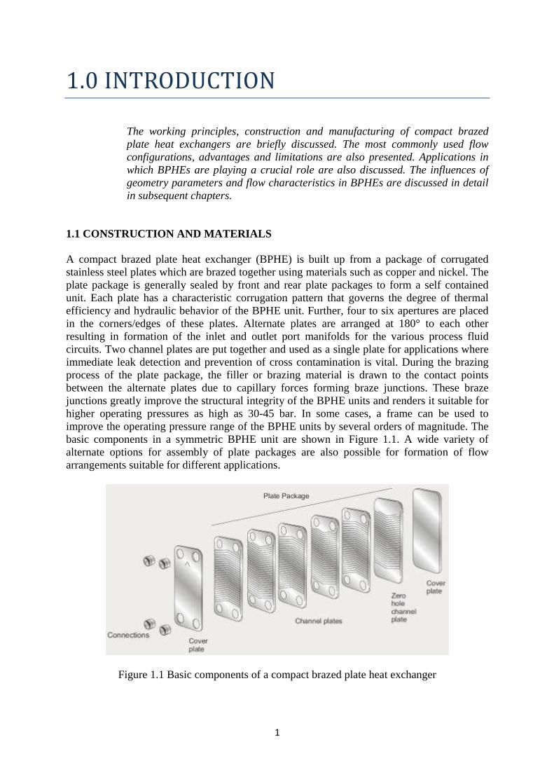
1.1 CONSTRUCTION AND MATERIALS A compact brazed plate heat exchanger (BPHE) is built up from a package of corrugated stainless steel plates which are brazed together using materials such as copper and nickel. The plate package is generally sealed by front and rear plate packages to form a self contained unit. Each plate has a characteristic corrugation pattern that governs the degree of thermal efficiency and hydraulic behavior of the BPHE unit. Further, four to six apertures are placed in the corners/edges of these plates. Alternate plates are arranged at 180° to each other resulting in formation of the inlet and outlet port manifolds for the various process fluid circuits. Two channel plates are put together and used as a single plate for applications where immediate leak detection and prevention of cross contamination is vital. During the brazing process of the plate package, the filler or brazing material is drawn to the contact points between the alternate plates due to capillary forces forming braze junctions. These braze junctions greatly improve the structural integrity of the BPHE units and renders it suitable for higher operating pressures as high as 30-45 bar. In some cases, a frame can be used to improve the operating pressure range of the BPHE units by several orders of magnitude. The basic components in a symmetric BPHE unit are shown in Figure 1.1. A wide variety of alternate options for assembly of plate packages are also possible for formation of flow arrangements suitable for different applications.

Figure 1.1 Basic components of a compact brazed plate heat exchanger

2

During the manufacturing process, the stainless steel and brazing material is fed from their respective coils, which are cut simultaneously and stacked into plate packs. These packs together with auxiliary parts such as distribution rings, blind rings etc., are assembled with the cover plates and the required connections. These stacked units loaded using dead weights or spring loaded weights are vacuum-brazed for about eight hours in furnaces. The methods of manufacturing brazed plate heat exchangers are continuously evolving with developments in areas such as modern brazing methods, research on alternative brazing materials and raw material forms of brazing materials. Various types of connections can be placed at the front or rear face depending on the market and application requirements. Blind rings and additional sealing plates are usually used to separate the cover plates from the channel plates. The dimensions and number of the cover plates depend on the application. Directional information for mounting of the heat exchangers is also provided. This is required to identify the number and location of channels connected for a given process fluid steam. The standard BPHEs are built from AISI316 steel with copper as brazing material and have a design pressure of around 31 bar. Nickel is used as brazing material in applications where copper presents compatibility problem with process fluids. SMO254 and AISI 304 steel variants are also used for channel plates in some applications. External/internal threaded, Rotalock, flanged and solder connections are generally provided. Further information on classification plate type heat exchangers, their construction and manufacturing methods can be found in Wang et al. (2007) 1.2 FLOW AND CIRCUIT ARRANGEMENT The flow direction and circuit arrangement in BPHEs is governed by application parameters such as desired thermal length, available temperature difference, allowable pressure drop, and other restrictions arising from fluid physical properties. Counter flow arrangement, in which fluids in alternate channels flow in opposite directions, is generally preferred due to efficient use of available temperature difference. However, parallel flow arrangement offers significant advantages for cases where pure phase-change or constant temperature or latent heat transfer is involved. In such circumstances, parallel flow arrangement generally requires lower heat transfer area because the temperature difference penalty due to pressure drop renders counter flow inefficient. Pure counter flow is not achievable in BPHEs due to factors such as port locations and fluid flow paths in the alternate channels. However, the degree of counter-flow increases with increasing plate aspect ratio (length to width ratio) and with better in-channel distribution. In plate designs with larger aspect ratios, pure cross-flow arrangement can be achieved. Cross-flow brazed plate heat exchangers are generally asymmetric (alternate channels have different thermal and hydraulic behavior) because the channel characteristics are governed by the angle of corrugation pattern to the main flow direction. The most common flow arrangement is a loop arrangement where each process fluid is split into parts and is distributed into alternate channels from the port manifolds. Thus the process fluid on each circuit flows in the same direction and this arrangement is termed as single pass arrangement. As inferred from Figure 1.1, the outer most channels have heat transfer in only one direction and this introduces a non-uniform temperature profile in various channels. This non-uniformity is considered by approximate models during heat exchanger calculations and this influence becomes negligible in plate packages greater than 20 plates. The distribution of the fluid from the port manifold to the channels is governed by the magnitude of the channel pressure drop, friction losses in the port and momentum changes due to change of velocities in the inlet and outlet ports. An ideal channel distribution is desired to effectively use the available heat transfer area. The distribution plays an extremely important role in plate evaporators and this is generally improved using auxiliary devices such as distribution rings

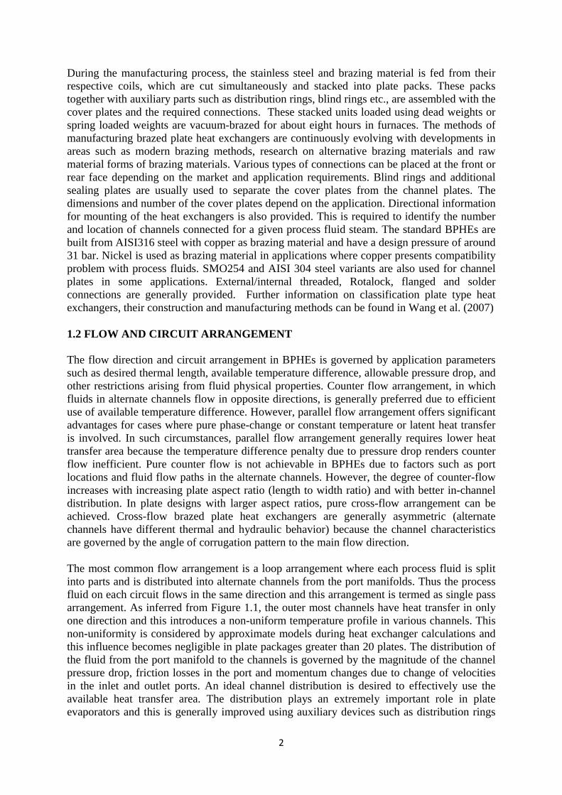
and other devices. The location of the connections for a circuit results distributions, namely, the U and Z arrangement. In the U arrangement, the inlet and outlet connections exist on same side and this is only valid for single pass heat exchangers. In the Z arrangement, the connections exist on the opposite enapplications, the Z arrangement offers better flow distribution due to its symmetric nature. The dimensions of the ports and connections are governed by factors such as allowable pressure drop, distribution parameters an In certain applications, thermal length requirements need the fluid stream to undergo the heat transfer process for a longer duration following a longer path. Multithe fluid from a single circuit flows exchangers are required for these applications. Such multipossible using blind rings in places where the fluids stream needs to change direction. Up to six passes are generallyarrangement in brazed plate heat exchangers is shown in Figure 1.2. The multiarrangement enhances the thermal length (number of transfer units) of a fluid stream but is associated with slength. Thermal efficiency is slightly reduced due to presence of parallel flow circuits at the onset of every pass. This reduction becomes insignificant with decreasing number oand increasing number of plates. All of the fluid streams in brazed plate heat exchangers do not require havingstringent allowable pressure drop requirements exist on one of the sides, it is customary to use asymmetric number of passes for both the sides.

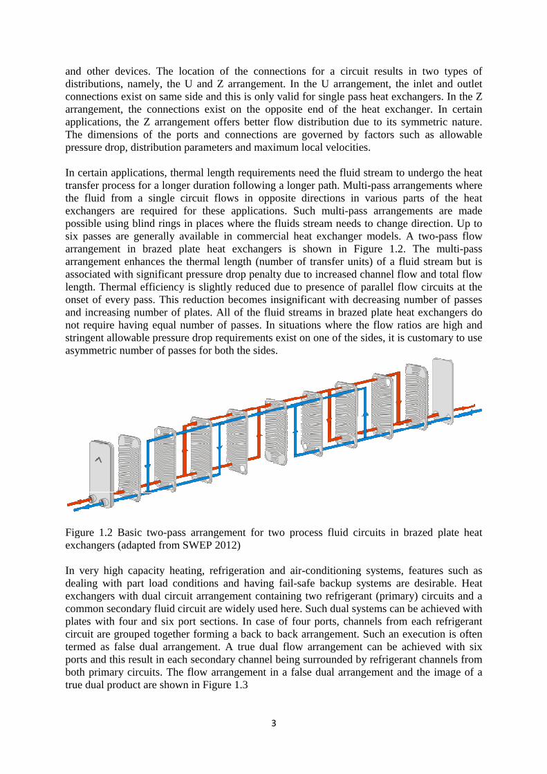
Figure 1.2 Basic twoexchangers (adapted from SWEP 2012) In very high capacity heating, refrigeration and airdealing with part load conditions and having failexchangers with dual circuit arrangement containing two refrigerant (primary) circuits and a common secondary fluid circuit are widely used here. Such dual systems can be achieved with plates with four and six port sections. In casecircuit are grouped together forming a back to back arrangement. Such an execution is often termed as false dual arrangement. A true dual flow arrangement can be achieved with six ports and this result in eachboth primary circuits. The flow arrangement in a false dual arrangement and the image of a true dual product are shown in Figure 1.3

3

and other devices. The location of the connections for a circuit results distributions, namely, the U and Z arrangement. In the U arrangement, the inlet and outlet connections exist on same side and this is only valid for single pass heat exchangers. In the Z arrangement, the connections exist on the opposite enapplications, the Z arrangement offers better flow distribution due to its symmetric nature. The dimensions of the ports and connections are governed by factors such as allowable pressure drop, distribution parameters and maximum local velocities.

In certain applications, thermal length requirements need the fluid stream to undergo the heat transfer process for a longer duration following a longer path. Multithe fluid from a single circuit flows in opposite directions in various parts of the heat exchangers are required for these applications. Such multipossible using blind rings in places where the fluids stream needs to change direction. Up to six passes are generally available in commercial heat exchanger models. A twoarrangement in brazed plate heat exchangers is shown in Figure 1.2. The multiarrangement enhances the thermal length (number of transfer units) of a fluid stream but is associated with significant pressure drop penalty due to increased channel flow and total flow length. Thermal efficiency is slightly reduced due to presence of parallel flow circuits at the onset of every pass. This reduction becomes insignificant with decreasing number oand increasing number of plates. All of the fluid streams in brazed plate heat exchangers do

having equal number of passes. In situations where the flow ratios are high and stringent allowable pressure drop requirements exist on one of the sides, it is customary to use asymmetric number of passes for both the sides.

Figure 1.2 Basic two-pass arrangement for two process fluid circuits in brazed plate heat exchangers (adapted from SWEP 2012)

In very high capacity heating, refrigeration and airdealing with part load conditions and having failexchangers with dual circuit arrangement containing two refrigerant (primary) circuits and a common secondary fluid circuit are widely used here. Such dual systems can be achieved with plates with four and six port sections. In case circuit are grouped together forming a back to back arrangement. Such an execution is often termed as false dual arrangement. A true dual flow arrangement can be achieved with six ports and this result in each secondary channel being surrounded by refrigerant channels from both primary circuits. The flow arrangement in a false dual arrangement and the image of a true dual product are shown in Figure 1.3

3

and other devices. The location of the connections for a circuit results in two types of distributions, namely, the U and Z arrangement. In the U arrangement, the inlet and outlet connections exist on same side and this is only valid for single pass heat exchangers. In the Z arrangement, the connections exist on the opposite end of the heat exchanger. In certain applications, the Z arrangement offers better flow distribution due to its symmetric nature. The dimensions of the ports and connections are governed by factors such as allowable

d maximum local velocities.

In certain applications, thermal length requirements need the fluid stream to undergo the heat transfer process for a longer duration following a longer path. Multi-pass arrangements where

in opposite directions in various parts of the heat exchangers are required for these applications. Such multi-pass arrangements are made possible using blind rings in places where the fluids stream needs to change direction. Up to

available in commercial heat exchanger models. A twoarrangement in brazed plate heat exchangers is shown in Figure 1.2. The multiarrangement enhances the thermal length (number of transfer units) of a fluid stream but is

ignificant pressure drop penalty due to increased channel flow and total flow length. Thermal efficiency is slightly reduced due to presence of parallel flow circuits at the onset of every pass. This reduction becomes insignificant with decreasing number oand increasing number of plates. All of the fluid streams in brazed plate heat exchangers do

equal number of passes. In situations where the flow ratios are high and stringent allowable pressure drop requirements exist on one of the sides, it is customary to use asymmetric number of passes for both the sides.

angement for two process fluid circuits in brazed plate heat

In very high capacity heating, refrigeration and air-conditioning systems, features such as dealing with part load conditions and having fail-safe backup systems are desirable. Heat exchangers with dual circuit arrangement containing two refrigerant (primary) circuits and a common secondary fluid circuit are widely used here. Such dual systems can be achieved with

of four ports, channels from each refrigerant circuit are grouped together forming a back to back arrangement. Such an execution is often termed as false dual arrangement. A true dual flow arrangement can be achieved with six

secondary channel being surrounded by refrigerant channels from both primary circuits. The flow arrangement in a false dual arrangement and the image of a

in two types of distributions, namely, the U and Z arrangement. In the U arrangement, the inlet and outlet connections exist on same side and this is only valid for single pass heat exchangers. In the Z

d of the heat exchanger. In certain applications, the Z arrangement offers better flow distribution due to its symmetric nature. The dimensions of the ports and connections are governed by factors such as allowable

In certain applications, thermal length requirements need the fluid stream to undergo the heat pass arrangements where

in opposite directions in various parts of the heat pass arrangements are made

possible using blind rings in places where the fluids stream needs to change direction. Up to available in commercial heat exchanger models. A two-pass flow

arrangement in brazed plate heat exchangers is shown in Figure 1.2. The multi-pass arrangement enhances the thermal length (number of transfer units) of a fluid stream but is

ignificant pressure drop penalty due to increased channel flow and total flow length. Thermal efficiency is slightly reduced due to presence of parallel flow circuits at the onset of every pass. This reduction becomes insignificant with decreasing number of passes and increasing number of plates. All of the fluid streams in brazed plate heat exchangers do

equal number of passes. In situations where the flow ratios are high and stringent allowable pressure drop requirements exist on one of the sides, it is customary to use

angement for two process fluid circuits in brazed plate heat

conditioning systems, features such as ems are desirable. Heat

exchangers with dual circuit arrangement containing two refrigerant (primary) circuits and a common secondary fluid circuit are widely used here. Such dual systems can be achieved with

of four ports, channels from each refrigerant circuit are grouped together forming a back to back arrangement. Such an execution is often termed as false dual arrangement. A true dual flow arrangement can be achieved with six

secondary channel being surrounded by refrigerant channels from both primary circuits. The flow arrangement in a false dual arrangement and the image of a

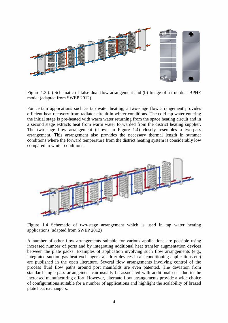
Figure 1.3 (a) Schematic of false dual flow model (adapted from SWEP 2012) For certain applications such as tap water heating, a twoefficient heat recovery from radiator circuit in winter conditions. The cold tap water ethe initial stage is prea second stage extracts heat from warm water forwarded from the district heating supplier. The two-stage flow arrangement (shown in arrangement. This arrangement also provides the necessary thermal length in summer conditions where the forward temperature from the district heating system icompared to winter conditions.

Figure 1.4 Schematic of tapplications (adapted from SWEP 2012) A number of other flow arrangements suitable for various applications are possible using increased number of ports and by integrating additional heat transfer aubetween the plate packs. Examples of application involving such flow arrangements (e.g.integrated suction gas heat exchangers, airare published in process fluid flow paths around port manifolds are even patented. The deviation from standard single-pass arrangement can usually be associated with additional cost due to the increased manufacturing effort. However, alof configurations suitable for a number of applications and highlight the scalability of brazed plate heat exchangers.

4

Figure 1.3 (a) Schematic of false dual flow arrangement and (b) Image of a true dual BPHE model (adapted from SWEP 2012)

For certain applications such as tap water heating, a twoefficient heat recovery from radiator circuit in winter conditions. The cold tap water ethe initial stage is pre-heated with warm water returning from the space heating circuit and in a second stage extracts heat from warm water forwarded from the district heating supplier.

stage flow arrangement (shown in arrangement. This arrangement also provides the necessary thermal length in summer conditions where the forward temperature from the district heating system icompared to winter conditions.

Figure 1.4 Schematic of two-stage arrangement which is used in tap water heating applications (adapted from SWEP 2012)

A number of other flow arrangements suitable for various applications are possible using increased number of ports and by integrating additional heat transfer aubetween the plate packs. Examples of application involving such flow arrangements (e.g.integrated suction gas heat exchangers, air-drier devices in airare published in the open literature. Several flow aprocess fluid flow paths around port manifolds are even patented. The deviation from

pass arrangement can usually be associated with additional cost due to the increased manufacturing effort. However, alternate flow arrangements provide a wide choice of configurations suitable for a number of applications and highlight the scalability of brazed plate heat exchangers.

4

arrangement and (b) Image of a true dual BPHE

For certain applications such as tap water heating, a two-stage flow arrangement provides efficient heat recovery from radiator circuit in winter conditions. The cold tap water e

heated with warm water returning from the space heating circuit and in a second stage extracts heat from warm water forwarded from the district heating supplier.

stage flow arrangement (shown in Figure 1.4) closely resembles a twoarrangement. This arrangement also provides the necessary thermal length in summer conditions where the forward temperature from the district heating system is considerably low

stage arrangement which is used in tap water heating

A number of other flow arrangements suitable for various applications are possible using increased number of ports and by integrating additional heat transfer augmentation devices between the plate packs. Examples of application involving such flow arrangements (e.g.

drier devices in air-conditioning applications etc) open literature. Several flow arrangements involving control of the

process fluid flow paths around port manifolds are even patented. The deviation from pass arrangement can usually be associated with additional cost due to the

ternate flow arrangements provide a wide choice of configurations suitable for a number of applications and highlight the scalability of brazed

arrangement and (b) Image of a true dual BPHE

stage flow arrangement provides efficient heat recovery from radiator circuit in winter conditions. The cold tap water entering

heated with warm water returning from the space heating circuit and in a second stage extracts heat from warm water forwarded from the district heating supplier.

resembles a two-pass arrangement. This arrangement also provides the necessary thermal length in summer

considerably low

stage arrangement which is used in tap water heating

A number of other flow arrangements suitable for various applications are possible using gmentation devices

between the plate packs. Examples of application involving such flow arrangements (e.g., conditioning applications etc)

rrangements involving control of the process fluid flow paths around port manifolds are even patented. The deviation from

pass arrangement can usually be associated with additional cost due to the ternate flow arrangements provide a wide choice

of configurations suitable for a number of applications and highlight the scalability of brazed

5

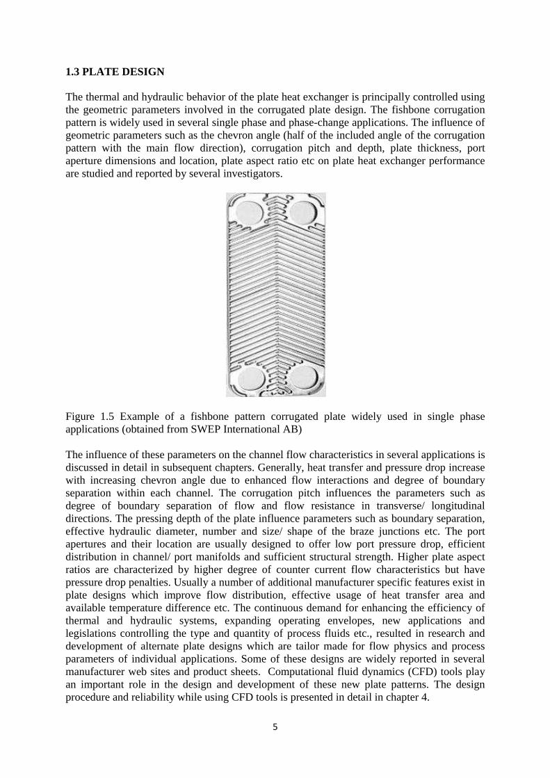
1.3 PLATE DESIGN The thermal and hydraulic behavior of the plate heat exchanger is principally controlled using the geometric parameters involved in the corrugated plate design. The fishbone corrugation pattern is widely used in several single phase and phase-change applications. The influence of geometric parameters such as the chevron angle (half of the included angle of the corrugation pattern with the main flow direction), corrugation pitch and depth, plate thickness, port aperture dimensions and location, plate aspect ratio etc on plate heat exchanger performance are studied and reported by several investigators.

Figure 1.5 Example of a fishbone pattern corrugated plate widely used in single phase applications (obtained from SWEP International AB) The influence of these parameters on the channel flow characteristics in several applications is discussed in detail in subsequent chapters. Generally, heat transfer and pressure drop increase with increasing chevron angle due to enhanced flow interactions and degree of boundary separation within each channel. The corrugation pitch influences the parameters such as degree of boundary separation of flow and flow resistance in transverse/ longitudinal directions. The pressing depth of the plate influence parameters such as boundary separation, effective hydraulic diameter, number and size/ shape of the braze junctions etc. The port apertures and their location are usually designed to offer low port pressure drop, efficient distribution in channel/ port manifolds and sufficient structural strength. Higher plate aspect ratios are characterized by higher degree of counter current flow characteristics but have pressure drop penalties. Usually a number of additional manufacturer specific features exist in plate designs which improve flow distribution, effective usage of heat transfer area and available temperature difference etc. The continuous demand for enhancing the efficiency of thermal and hydraulic systems, expanding operating envelopes, new applications and legislations controlling the type and quantity of process fluids etc., resulted in research and development of alternate plate designs which are tailor made for flow physics and process parameters of individual applications. Some of these designs are widely reported in several manufacturer web sites and product sheets. Computational fluid dynamics (CFD) tools play an important role in the design and development of these new plate patterns. The design procedure and reliability while using CFD tools is presented in detail in chapter 4.

6

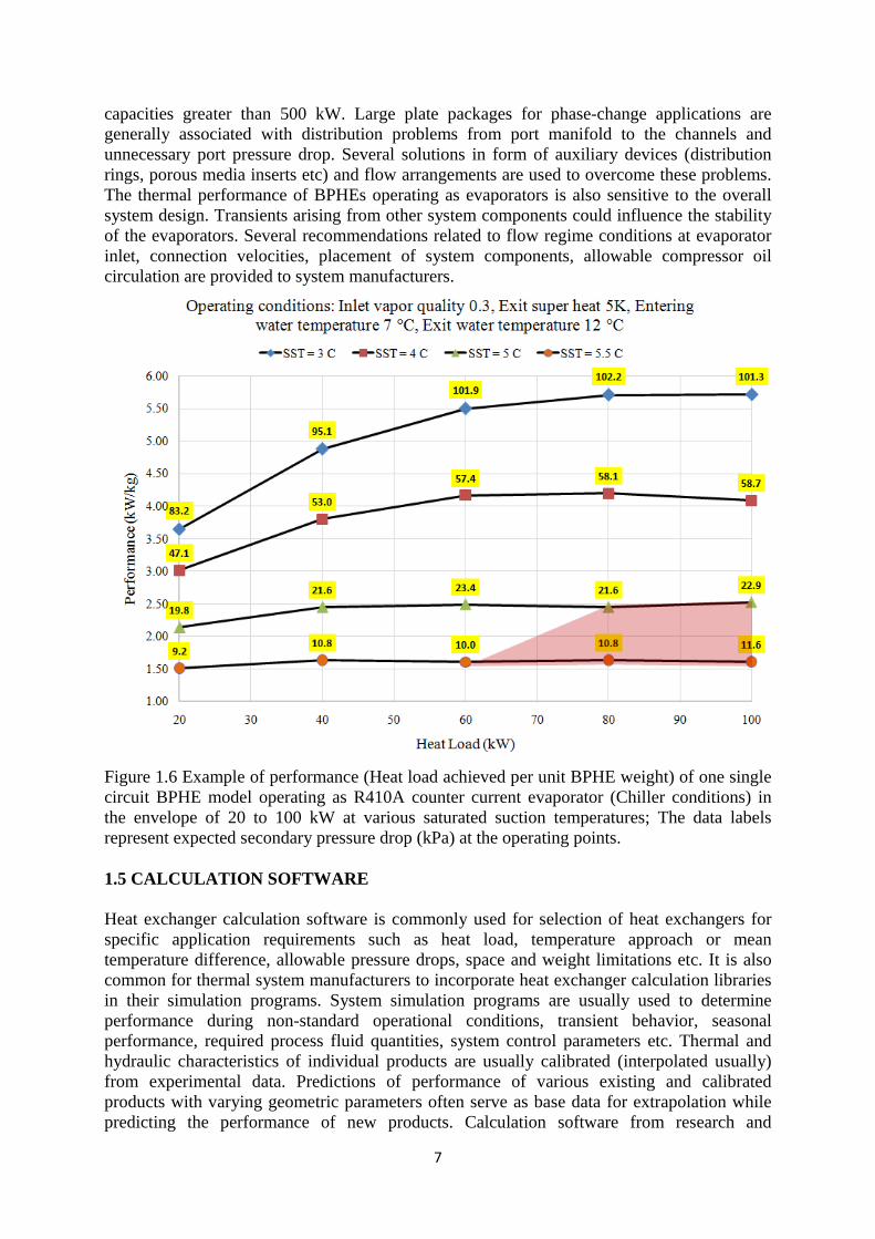
1.4 APPLICATIONS AND ADVANTAGES Compactness, low volume, scalability, possibility to achieve close temperature approaches, relatively high values of the heat transfer coefficients make brazed plate heat exchangers suitable for a very wide range of applications. Single phase applications such as district heating and cooling, demand very close temperature approaches and best use of the forwarding temperatures from the energy supplier while offering lower pressure losses. Brazed plate heat exchangers with flexible plate and pass arrangement are a suitable choice here. Asymmetric channel designs offer fluid circuits with varying degree of thermal efficiency and hydraulic characteristics that are observed in these applications. BPHEs are typically used as radiator and two-stage tap water heat exchanger in district heating sub-stations. Other single phase applications include oil cooling in wind power generation systems, engine oil cooling in ship engines, oil cooling for heat recovery, co-generation, super-critical gas cooling, and heat recovery applications in refrigeration systems etc. The complex flow paths in plate heat exchangers lower the critical Reynolds number for the onset of turbulence significantly and this makes them suitable for applications involving high viscous fluids. Typical mass flux conditions for single phase applications are in the order of 100 kg / (m² s) with heat flux in the range of 50-100 kW/m². The secondary flows, degree of mixing and friction loss result in sufficient magnitude of shear stress on the heat transfer surfaces and this inhibits fouling to a great extent. Super-critical CO2 gas cooling process in space and tap water heating applications require larger thermal length to overcome the close temperature approaches involved in these applications. Operating pressures in these applications are in the range of 90-140 bar. Port areas and edges of BPHEs are generally designed using non-standard features in order to withstand such higher operating pressures. Plate heat exchangers are widely used for phase-change heat transfer in refrigeration, residential heating and air-conditioning applications. The mass flux for these applications is typically in the order of 50 kg/ (m² s) with a heat flux range of 1 – 20 kW/m². Phase change applications include evaporators, condensers, sub-coolers and economizers etc. In super- market refrigeration systems, BPHEs are used as cascaded heat exchangers with evaporation and condensation occurring in the same unit. Example of performance (heat load achieved per unit BPHE weight) of a BPHE model operating as an evaporator at normal chiller rating conditions is shown in Figure 1.6. Alternate applications such as power generation using Organic Rankine Cycle, integrated air drying systems, absorption chillers also use brazed plate heat exchangers. In phase-change applications, the thermal restriction generally lies on the refrigerant side. The averaged heat transfer coefficients on the refrigerant side are many times lower than those on the secondary side. The pressure drop on the secondary side is also required to be maintained as low as possible. These requirements call for asymmetric designs with increased channel velocity in refrigerant channels and decreased pressure drop on secondary sides. At lower operating pressures, refrigerant pressure drop causes a temperature difference penalty and this governs the degree of asymmetry possible for a given application. The weight and volume of BPHEs are generally 20 -30% less than those for traditional shell and tube heat exchangers and this reduces the overall foot-print of the system greatly. Relatively small internal volume reduces the required refrigerant charge in phase-change applications. The total height of the BPHEs is currently limited to 1.5 meters due to restrictions of the brazing process. However, BPHEs are suitable for wide capacity and application ranges due to the scalability and possible flow arrangements. In phase-change applications BPHEs currently can deliver temperature approaches lower than 1K and

7

capacities greater than 500 kW. Large plate packages for phase-change applications are generally associated with distribution problems from port manifold to the channels and unnecessary port pressure drop. Several solutions in form of auxiliary devices (distribution rings, porous media inserts etc) and flow arrangements are used to overcome these problems. The thermal performance of BPHEs operating as evaporators is also sensitive to the overall system design. Transients arising from other system components could influence the stability of the evaporators. Several recommendations related to flow regime conditions at evaporator inlet, connection velocities, placement of system components, allowable compressor oil circulation are provided to system manufacturers.

Figure 1.6 Example of performance (Heat load achieved per unit BPHE weight) of one single circuit BPHE model operating as R410A counter current evaporator (Chiller conditions) in the envelope of 20 to 100 kW at various saturated suction temperatures; The data labels represent expected secondary pressure drop (kPa) at the operating points. 1.5 CALCULATION SOFTWARE Heat exchanger calculation software is commonly used for selection of heat exchangers for specific application requirements such as heat load, temperature approach or mean temperature difference, allowable pressure drops, space and weight limitations etc. It is also common for thermal system manufacturers to incorporate heat exchanger calculation libraries in their simulation programs. System simulation programs are usually used to determine performance during non-standard operational conditions, transient behavior, seasonal performance, required process fluid quantities, system control parameters etc. Thermal and hydraulic characteristics of individual products are usually calibrated (interpolated usually) from experimental data. Predictions of performance of various existing and calibrated products with varying geometric parameters often serve as base data for extrapolation while predicting the performance of new products. Calculation software from research and

8

academic institutions usually are based on generalized thermal and hydraulic correlations derived for classical empirical equations (usually derived for pipe flow) and further adjustments based on limited experimental data. Product specific interpolated correlations are usually used in manufacturer provided software for improved predictions in the recommended product envelope. Accuracy, robustness, seamless integration with other programs, generality and speed are desirable characteristics of calculation software. The choice of correlations and calculation methods should aim at meeting these requirements. Commonly used single phase and phase-change thermal and hydraulic correlations, two-phase flow equations are presented in Chapter 2. Various calculation methods, discretization schemes, fluid property calculation methods, laboratory data evaluation are discussed in Chapter 3. REFERENCES Wang, L., Sundén, B., and Manglik, R.M., Plate Heat Exchangers: Design, Applications and Performance, WIT Press, ISBN 978-1-85312-737-3, 2007. SWEP International AB, BPHE Hand Book, 2012 (http://www.swep.net)

9

2.0 PLATE HEAT EXCHANGER THEORY

The chapter presents summary of the heat exchanger calculation methods such as LMTD and Effectiveness-NTU methods that are used in the current study during the evaluation of heat transfer and pressure drop correlations. A summary of a literature study on heat transfer and pressure drop in single-phase and two-phase mode in plate heat exchangers is presented. Other issues such as void fraction models and flow mechanism in plate heat exchanger channels are briefly discussed.

2.1 HEAT EXCHANGER CALCULATIONS Heat exchanger calculations developed for software applications such as selection programs and refrigeration system simulation programs can be classified broadly as: Rating calculations: Used to determine the suitability of a given heat exchanger for given thermal and hydraulic duties. The output in these calculations is over surface (ratio of area available to area required) and pressure drops. Performance calculations: Used to determine missing parameters, for example, outlet temperatures when the heat exchanger dimensions and some parameters are specified. Selection calculations: Used to determine the dimensions of a heat exchanger type (number of plates, number of passes, parallel units, flow arrangements, connections etc) that suits given thermal and hydraulic requirements. Two standard lumped methods for heat exchanger thermal performance analyses are used in this work and they are discussed here. 2.1.1 Logarithmic Mean Temperature Difference (LMTD) method This method serves as a basis for rating calculations because it calculates the required overall heat transfer coefficient for a given heat load and temperature profile. The total heat load in the CBE is derived as a product of the overall heat transfer coefficient, effective heat transfer area and the logarithmic mean temperature difference.

( )1 2

1 2ln /

T TQ U A

T T

∆ − ∆= Ω ∆ ∆ (2.1)

The correction factor Ω is used to adjust the performance for conditions such as multi-pass flow arrangement and for non uniform heat transfer at the end plates. This factor approaches unity as the number of plates increase and the number of passes decrease. Because equation (2.1) can be used to compare the area available and area required, this method can be used to determine over surface in rating calculations. The performance and selection calculations then iteratively use the rating calculation to determine missing parameters and the BPHE dimensions, respectively. This methodology is described in detail

10

in Incropera et al. (1990). This method is sensitive and demands high accuracy in laboratory measurements at close temperature approaches. 2.1.2 Effectiveness – Number of Transfer Units Method The effectiveness of a heat exchanger is presented as the ratio of the actual and maximum possible heat transfer. The maximum possible heat transfer occurs in counter flow with an infinite flow length in cases where local temperatures are not dependent on local pressures. The minimum heat capacity flow rate of the two sides is used in determining the maximum heat transfer.

( )( ) ( )

( )( ) ( )max , , , ,min min

p h p ch c

p h in c in p h in c in

mC T mC TQ

Q mC T T mC T Tε

∆ ∆= = =

− −

ɺ ɺ

ɺ ɺ (2.2)

The effectiveness is related to the number of transfer units by a non-dimensional relation that is specific for a certain flow arrangement.

( )( )

min

max

,p

p

mCNTU

mCε

= Γ

ɺ

ɺ (2.3)

( )minp

UANTU

mC=

ɺ (2.4) This non-dimensional relation for the effectiveness is used for determining the missing parameters in performance calculations, without the need of iterative rating calculations. Various equations used in effectiveness-NTU based performance calculations are presented in Incropera et al. (1990).

( )( )

, , min

, , max

1 1ph out c out

h in c in p

mCT T

T T mCε − = − + −

ɺ

ɺ (2.5) 2.2 SINGLE PHASE APPLICATIONS Single phase heat transfer in plate heat exchangers is extensively studied by a number of researchers and is usually presented as a function of non-dimensional groups involving plate geometric features and fluid properties. These relations play a key role in the prediction of two-phase applications because the evaporation and condenser correlations usually involve contributions which are simply represented as enhanced single phase heat transfer term. Correlations proposed in the literature are summarized, for example, in Wang et al. (2007) and Ayub et al. (2003). Some of these correlations are presented below. Muley and Manglik (1997) studied mixed plate arrangements for chevron angles 30° and 60° with vegetable oil (130 < Pr < 220) and water (2.4 < Pr < 4.5) and presented the following correlations.

11

( )( )

0.140.5 1/3

0.140.76 1/3

0.471Re Pr 20 Re 400

0.1Re Pr Re 1000

wall

wall

Nuµ µ

µ µ

≤ <= > (2.6)

and

( ) ( )0.255 0.5

0.15

40.32 Re 8.12Re 2 Re 200

1.274Re Re 1000

f

−−

−

+ ≤ ≤ = ≥ (2.7)

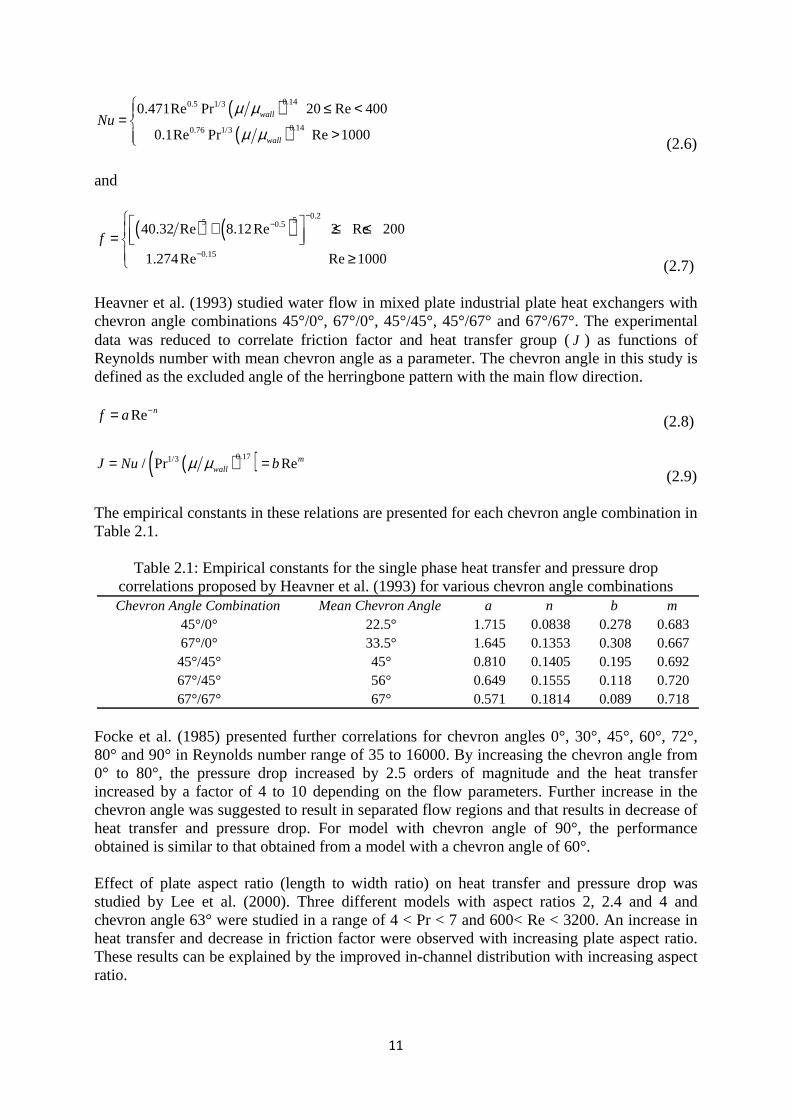
Heavner et al. (1993) studied water flow in mixed plate industrial plate heat exchangers with chevron angle combinations 45°/0°, 67°/0°, 45°/45°, 45°/67° and 67°/67°. The experimental data was reduced to correlate friction factor and heat transfer group (J ) as functions of Reynolds number with mean chevron angle as a parameter. The chevron angle in this study is defined as the excluded angle of the herringbone pattern with the main flow direction.

Re nf a −= (2.8)

( )( )0.171/3/ Pr RemwallJ Nu bµ µ= =

(2.9)

The empirical constants in these relations are presented for each chevron angle combination in Table 2.1.

Table 2.1: Empirical constants for the single phase heat transfer and pressure drop correlations proposed by Heavner et al. (1993) for various chevron angle combinations

Focke et al. (1985) presented further correlations for chevron angles 0°, 30°, 45°, 60°, 72°, 80° and 90° in Reynolds number range of 35 to 16000. By increasing the chevron angle from 0° to 80°, the pressure drop increased by 2.5 orders of magnitude and the heat transfer increased by a factor of 4 to 10 depending on the flow parameters. Further increase in the chevron angle was suggested to result in separated flow regions and that results in decrease of heat transfer and pressure drop. For model with chevron angle of 90°, the performance obtained is similar to that obtained from a model with a chevron angle of 60°. Effect of plate aspect ratio (length to width ratio) on heat transfer and pressure drop was studied by Lee et al. (2000). Three different models with aspect ratios 2, 2.4 and 4 and chevron angle 63° were studied in a range of 4 < Pr < 7 and 600< Re < 3200. An increase in heat transfer and decrease in friction factor were observed with increasing plate aspect ratio. These results can be explained by the improved in-channel distribution with increasing aspect ratio.

Chevron Angle Combination Mean Chevron Angle a n b m45°/0° 22.5° 1.715 0.0838 0.278 0.68367°/0° 33.5° 1.645 0.1353 0.308 0.66745°/45° 45° 0.810 0.1405 0.195 0.69267°/45° 56° 0.649 0.1555 0.118 0.72067°/67° 67° 0.571 0.1814 0.089 0.718

12

In the current study, a correlation due to Bogaert et al. (1994) is used for evaluating heat transfer correlation in single phase flow.

RePr Pr

z

nhy y

wall

hDNuC

µλ µ

= =

(2.10)

The Prandtl number exponent (y ) and the viscosity ratio exponent (z ) are correlated as functions of Prandtl number and Reynolds number, respectively, from a large set of experimental data. These relations cannot be presented in this article due to confidentiality terms. The pressure drop is modeled using standard Darcy friction factor model

2 2

Re2 2

m

h h

u L u LP f b

D D

ρ ρ−∆ = = (2.11)

The fluid properties are determined at mean temperatures in lumped analysis and at local thermodynamic state in discretized analysis. The empirical constants in the above equations are evaluated individually for various BPHE models by methods outlined in Chapter 3. 2.3 CONDENSATION IN PLATE HEAT EXCHANGERS The high heat transfer rates attainable with a low volume and lower pressure drops at elevated pressures provide a distinct advantage for plate heat exchangers for condensing application. The boundary separations caused by the chevron pattern result in mixed flow, which improves the interfacial shear stress. The key factor in designing an optimum condenser involves optimum area usage in the desuperheating area, enhancement of turbulence in the two-phase zone and improved drainage characteristics in the subcooled liquid region. In plate heat exchangers, the main resistance lies on the refrigerant side and enhancement on this side plays a significant role in the improving the overall efficiency of the heat exchanger. Due to these characteristics and compactness plate heat exchangers are commonly used in refrigeration and air conditioning applications. Despite this, very limited information regarding the condensation in brazed plate heat exchangers is available in the published literature. The experimental data and correlations available in the literature lack generality for a wide range of conditions and refrigerants. Many of the studies involve 3-4 plates which form a single refrigerant channel and it is observed that the performance in these units vary largely as compared to standard units with number of plates greater than 20. There is also a wide range of definitions used for describing geometry characteristics such as effective heat transfer area, hydraulic diameter and flow length; and non-dimensional numbers such as Reynolds number etc. The data reduction methodology varies from work to work which results in a wide range of derived overall heat transfer coefficient for the test points. These limitations force the usage of simplified product specific semi-empirical thermal and hydraulic correlations for commercial heat exchanger software applications. A brief literature study for condensation is presented below. Condensation is generally classified into two regimes in a number of investigations on plate heat exchangers. Gravity controlled regime with a low relative velocity between vapor and liquid film (typically Re 800fo < ) and shear controlled regime where significant shear stress is

induced by high vapor velocity stream on the condenser film (typically Re 1000fo > ). Nusselt

theory derives the local heat transfer coefficient for downward condensation in a vertical

13

channel in the gravity controlled regime. In this method, linear temperature profiles are assumed in the condensate film and local sub-cooling effects are ignored.

0.3331.1 Regr fh Co −= (2.12)

( ) 0.3332

f f f f gCo gλ µ ρ ρ ρ−

= − (2.13)

The integrated heat transfer coefficient along the length of the plate is given by

0.3331.47 Regr fh Co −= (2.14)

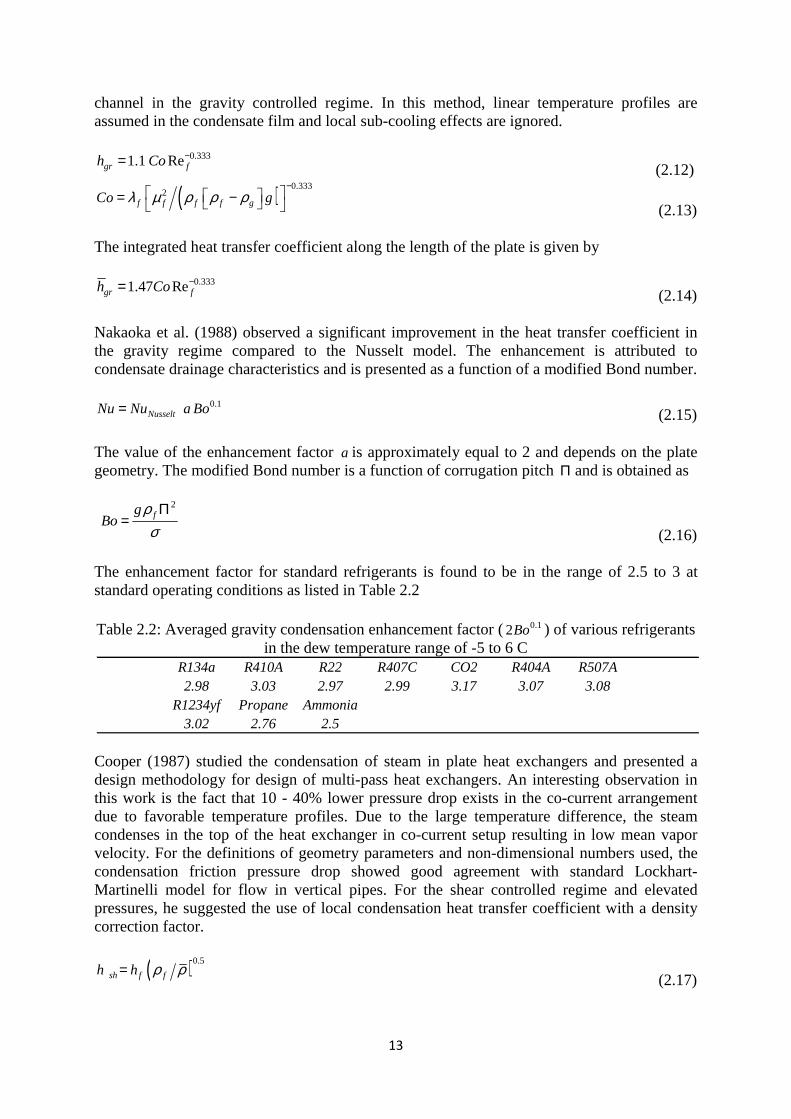
Nakaoka et al. (1988) observed a significant improvement in the heat transfer coefficient in the gravity regime compared to the Nusselt model. The enhancement is attributed to condensate drainage characteristics and is presented as a function of a modified Bond number.

0.1NusseltNu Nu a Bo= (2.15)

The value of the enhancement factor a is approximately equal to 2 and depends on the plate geometry. The modified Bond number is a function of corrugation pitch Π and is obtained as

2

fgBo

ρσ

Π=

(2.16) The enhancement factor for standard refrigerants is found to be in the range of 2.5 to 3 at standard operating conditions as listed in Table 2.2 Table 2.2: Averaged gravity condensation enhancement factor ( 0.12Bo ) of various refrigerants

in the dew temperature range of -5 to 6 C

Cooper (1987) studied the condensation of steam in plate heat exchangers and presented a design methodology for design of multi-pass heat exchangers. An interesting observation in this work is the fact that 10 - 40% lower pressure drop exists in the co-current arrangement due to favorable temperature profiles. Due to the large temperature difference, the steam condenses in the top of the heat exchanger in co-current setup resulting in low mean vapor velocity. For the definitions of geometry parameters and non-dimensional numbers used, the condensation friction pressure drop showed good agreement with standard Lockhart-Martinelli model for flow in vertical pipes. For the shear controlled regime and elevated pressures, he suggested the use of local condensation heat transfer coefficient with a density correction factor.

( )0.5

sh f fh h ρ ρ= (2.17)

R134a R410A R22 R407C CO2 R404A R507A2.98 3.03 2.97 2.99 3.17 3.07 3.08

R1234yf Propane Ammonia3.02 2.76 2.5

14

The method for calculating the mean density (ρ ) was not specified. The liquid heat transfer coefficient is calculated using a correlation similar to that by Bogaert. For the shear controlled regime, the correlation proposed by Shaw (1979) for condensation of steam, refrigerants and organics in pipes, which uses reduced pressureredP , is widely used.

( ) ( )0.040.760.80.8 0.4

0.38

3.8 10.023Re Pr 1sh h

f ff red

x xh Dx

Pλ

− = − + (2.18)

Thonon (1995 b) suggested that a correlation similar to the one proposed by Boyko – Kruzhilin (1967) should be used for condensation in shear controlled regime. The model requires evaluation of single phase heat transfer coefficient for a given plate geometry and should be suitable for developing product specific correlations.

0.5

1 1fsh f

g

h h xρρ

= + −

(2.19)

Because the transition is observed to occur smoothly between gravity and shear controlled regime, a root mean square value is calculated from the gravity and shear controlled regimes.

( )0.52 2co gr shh h h= +

(2.20)

For the gravity controlled regime, an enhancement factor (Fα ), is used together with equation (2.1) to account for the stirring effect at the liquid/ vapor interface. The values of this factor for different geometries are presented as a function of local vapor quality. In a study of condensation in a brazed plate heat exchanger using an elaborate 1D discretization model, Gullapalli (2007) derived Fα as a function of chevron angle. The values presented are 1.58, 1.67 and 2.24 for the chevron angles 47.5°, 61° and 67°, respectively. Study of evaporation and condensation in brazed plate heat exchangers using R22 and Propane was presented by Corberán (2000) et al. The work implies the importance of proper data reduction otherwise it was not possible to evaluate the correlation constants valid for wide range of testing conditions. Condensation of n-heptane and water in herringbone type plate heat exchanges was studied by Reinhard et al. (2004). Data is obtained from three channel tests with chevron angle combinations of 30°/30°, 60°/30° and 60°/60°. The plate spacing for these models is in the range of 2.5 to 7.4 mm. Experiments were conducted in the liquid Reynolds number range of 80 to 2000. Considerable deviations in heat transfer and pressure drop are observed compared to predictions from standard models. The choice of definition of geometric parameters and non-dimensional numbers might be the reason for deviation of predicted heat transfer coefficients and friction factors. For example, the area enhancement is not considered in the calculation of overall heat transfer area. The liquid Reynolds number is calculated as

( )Re 1

K

f heq

g l

DG x x

ρρ µ

= − +

(2.21)

15

and the condensation heat transfer coefficient is obtained using the relation

0.33.Re Prmco eq fNu C=

(2.22)

The two-phase friction pressure drop is predicted using the following empirical relation for turbulent – turbulent flow conditions.

20.5 0.10.9

, ,

1 g ffg F f F

f g

xP F P

x

ρ µρ µ

− − ∆ = ∆ (2.23)

The values of empirical constants are listed for all tested geometries. The proposed method predicted the measured overall heat transfer coefficient and pressure drop within an accuracy of ± 30%. The enhancement of the overall heat transfer coefficient compared to the Nusselt correlation is also presented. At liquid Reynolds number of 1000, an enhancement of around 1.8 is found for 30°/30° model and around 4.5 for 60°/60° model. Yan et al. (1999) published a correlation on heat transfer and pressure drop for condensation of R134a in a vertical plate heat exchanger. Only two vertical channels were considered in the study. Experiments were conducted with pure condensation in the channels without superheated vapor or sub-cooling and the standard LMTD was used in the data reduction. The heat transfer and pressure drop correlations are presented as

0.4 1/34.118Re Preq fNu = (2.24)

0.4 0.5 0.8 0.0467Re 94.75Reco red eqf Bo P− − −=

(2.25)

The boiling number used was defined as

( )fgBo q Gi= (2.26)

The equivalent Reynolds number is defined as in equation (2.21) with the value of the constant K is set to 0.5. Using these relations the heat transfer and pressure drop are predicted with an accuracy of ± 15%. Kuo et al. (2005) performed similar experiments on R410A in a three plates brazed plate heat exchanger with a chevron angle of 60°. Standard LMTD is used to derive the overall heat transfer coefficient and the condensation heat transfer coefficient and two-phase friction factors are presented as functions of mean vapor quality. The following correlation is presented for the friction factor.

1.14 0.08521500Reco eqf Bo− −= (2.27)

The heat transfer correlation is presented as enhancement of the single phase heat transfer coefficient.

16

( )0.45 0.25 0.750.25 75co f fh h CO Fr Bo−= + (2.28)

The definitions of equivalent Reynolds number and boiling number are similar to the analysis presented by Yan et al. (1999). The convection number and the Froude number are defined as

( ) ( ) 0.81g f m mCO x xρ ρ = − (2.29)

( )2 2f f hFr G gDρ=

(2.30)

Jokar et al. (2006) presented an elaborated study on condensation of R-134a in plate heat exchangers with an inter-plate spacing of 2 mm. The PHE unit with a chevron angle 60° was used. Three different plate numbers (34, 40 and 54 plates) were used in this study. The condensation heat transfer correlation is derived based on dimensional analysis with groups similar to Reynolds number, Nusselt number, Jacob number, Boiling number and vapor quality etc. The relation is presented as

1.3 1.05 0.05 2220.55 0.3

2 2,

3.371Re Pr f fg f fco f f

f f gf p f

iGNu

GC T G

ρ ρ σ ρµ ρ ρρ

=

−∆ (2.31)

The correlation might require an intensive evaluation process for individual refrigerants and plate heat exchanger models but is very interesting because it exhibits interesting considerations such as pressure dependence, local temperature difference, condensate drainage characteristics and buoyancy effects. Wang et al (2000) presented a correlation for steam condensation based on the Cooper correlation. The averaged condensation heat transfer coefficient is derived as

(2.32)

( ) Recfa b

f mM ρ ρ+

= (2.33)

The values for the correction factor coΦ are presented for various chevron angles and flow arrangements. The ranges of the empirical constants a, b and c in the above equation are presented as 0.3 to 0.37, 5.0 to 6.0 and -0.6 to -0.64, respectively. Among the presented correlations, the one used by Thonon (1995) appears to be more suitable for development of databases for commercial BPHE performance prediction applications. The correlation presented by Jokar et al. (2006) is very interesting because it encapsulated various influences on the condensing process in plate heat exchanger channels. However, additional correction factors might be required to compensate for the geometry and production method variations between different manufacturers.

( )co f in out coh h M M= + Φ

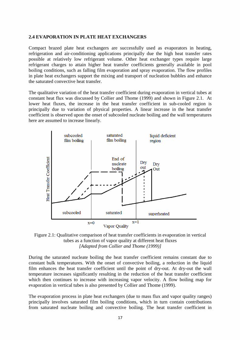
2.4 EVAPORATION IN PLATE HEAT EXCHANGERS Compact brazed plate heat exchangers are successfully used as evaporators in heating, refrigeration and airpossible at relatirefrigerant charges to attain higher heat transfer coefficients generally available in pool boiling conditions, such as falling film evaporation and spray evaporation. The flow profiles in plate heat exchangers support the mixing and transport of nucleation bubbles and enhance the saturated convective heat transfer. The qualitative variation of the heat transfer coefficient during evaporation in vertical tubes at constant heat flux was dlower heat fluxes, the increase in the heat transfer coefficient in subprincipally due to variation of physical properties. A linear increase in the heat transfer coefficient is observed upon the onset of subcooled nucleate boiling and the wall temperatures here are assumed to increase linearly.

Figure 2.1: Qualitative comparison of heat transfer coefficients in evaporation in vertical

During the saturated nucleate boiling the heat transfer coefficient remains constant due to constant bulk temperatures. With the onset of convective boiling, a reduction in the liquid film enhances the heat transfer coefficient until the point of drytemperature increases significantly resulting in the reduction of the heat transfer coefficient which then continues to increase with increasing vapor velocity. A flow evaporation in vertical tubes is also presented by Collier and Thome (1999) The evaporation process in plate heat exchangers (due to mass flux and vapor quality ranges) principally involves saturated film boiling conditions, which in turn contain contributions from saturated nucleate boiling and convective boiling. The heat transf

17

2.4 EVAPORATION IN PLATE HEAT EXCHANGERS

Compact brazed plate heat exchangers are successfully used as evaporators in heating, refrigeration and air-conditioning applications principally due the high heat transfer rates possible at relatively low refrigerant volume. Other heat exchanger types require large refrigerant charges to attain higher heat transfer coefficients generally available in pool boiling conditions, such as falling film evaporation and spray evaporation. The flow profiles in plate heat exchangers support the mixing and transport of nucleation bubbles and enhance the saturated convective heat transfer.

The qualitative variation of the heat transfer coefficient during evaporation in vertical tubes at constant heat flux was discussed by Collier and Thome (1999)lower heat fluxes, the increase in the heat transfer coefficient in subprincipally due to variation of physical properties. A linear increase in the heat transfer

nt is observed upon the onset of subcooled nucleate boiling and the wall temperatures here are assumed to increase linearly.

Figure 2.1: Qualitative comparison of heat transfer coefficients in evaporation in vertical tubes as a function of vapor qualit

[Adapted from Collier and Thome (1999)]

During the saturated nucleate boiling the heat transfer coefficient remains constant due to constant bulk temperatures. With the onset of convective boiling, a reduction in the liquid

enhances the heat transfer coefficient until the point of drytemperature increases significantly resulting in the reduction of the heat transfer coefficient which then continues to increase with increasing vapor velocity. A flow evaporation in vertical tubes is also presented by Collier and Thome (1999)

The evaporation process in plate heat exchangers (due to mass flux and vapor quality ranges) principally involves saturated film boiling conditions, which in turn contain contributions from saturated nucleate boiling and convective boiling. The heat transf

17

2.4 EVAPORATION IN PLATE HEAT EXCHANGERS

Compact brazed plate heat exchangers are successfully used as evaporators in heating, conditioning applications principally due the high heat transfer rates

vely low refrigerant volume. Other heat exchanger types require large refrigerant charges to attain higher heat transfer coefficients generally available in pool boiling conditions, such as falling film evaporation and spray evaporation. The flow profiles in plate heat exchangers support the mixing and transport of nucleation bubbles and enhance

The qualitative variation of the heat transfer coefficient during evaporation in vertical tubes at iscussed by Collier and Thome (1999) and shown in Figure 2.1

lower heat fluxes, the increase in the heat transfer coefficient in sub-cooled region is principally due to variation of physical properties. A linear increase in the heat transfer

nt is observed upon the onset of subcooled nucleate boiling and the wall temperatures

Figure 2.1: Qualitative comparison of heat transfer coefficients in evaporation in vertical tubes as a function of vapor quality at different heat fluxes

from Collier and Thome (1999)]

During the saturated nucleate boiling the heat transfer coefficient remains constant due to constant bulk temperatures. With the onset of convective boiling, a reduction in the liquid

enhances the heat transfer coefficient until the point of dry-out. At drytemperature increases significantly resulting in the reduction of the heat transfer coefficient which then continues to increase with increasing vapor velocity. A flow boiling map for evaporation in vertical tubes is also presented by Collier and Thome (1999).

The evaporation process in plate heat exchangers (due to mass flux and vapor quality ranges) principally involves saturated film boiling conditions, which in turn contain contributions from saturated nucleate boiling and convective boiling. The heat transfer coefficient in

Compact brazed plate heat exchangers are successfully used as evaporators in heating, conditioning applications principally due the high heat transfer rates

vely low refrigerant volume. Other heat exchanger types require large refrigerant charges to attain higher heat transfer coefficients generally available in pool boiling conditions, such as falling film evaporation and spray evaporation. The flow profiles in plate heat exchangers support the mixing and transport of nucleation bubbles and enhance

The qualitative variation of the heat transfer coefficient during evaporation in vertical tubes at and shown in Figure 2.1. At

cooled region is principally due to variation of physical properties. A linear increase in the heat transfer

nt is observed upon the onset of subcooled nucleate boiling and the wall temperatures

Figure 2.1: Qualitative comparison of heat transfer coefficients in evaporation in vertical

During the saturated nucleate boiling the heat transfer coefficient remains constant due to constant bulk temperatures. With the onset of convective boiling, a reduction in the liquid

out. At dry-out the wall temperature increases significantly resulting in the reduction of the heat transfer coefficient

boiling map for

The evaporation process in plate heat exchangers (due to mass flux and vapor quality ranges) principally involves saturated film boiling conditions, which in turn contain contributions

er coefficient in

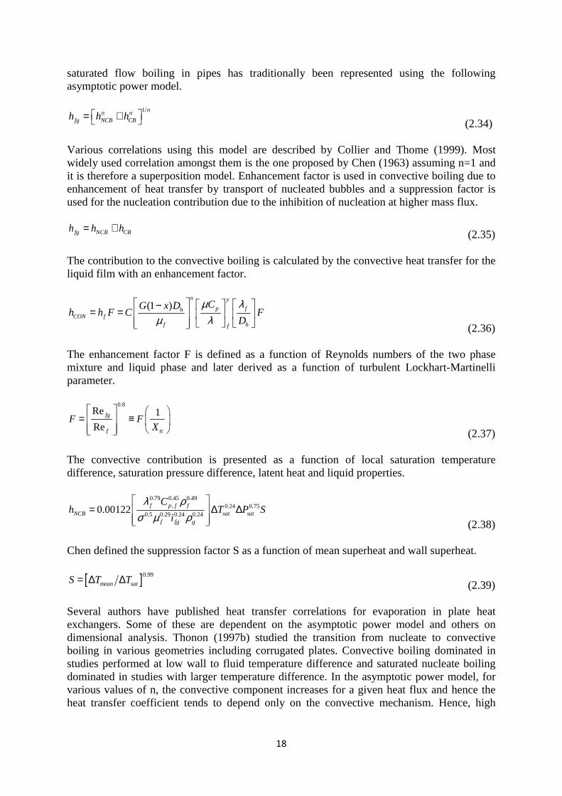
18

saturated flow boiling in pipes has traditionally been represented using the following asymptotic power model.

1/nn nfg NCB CBh h h = + (2.34)

Various correlations using this model are described by Collier and Thome (1999). Most widely used correlation amongst them is the one proposed by Chen (1963) assuming n=1 and it is therefore a superposition model. Enhancement factor is used in convective boiling due to enhancement of heat transfer by transport of nucleated bubbles and a suppression factor is used for the nucleation contribution due to the inhibition of nucleation at higher mass flux.

fg NCB CBh h h= + (2.35)

The contribution to the convective boiling is calculated by the convective heat transfer for the liquid film with an enhancement factor.

(1 )n y

p fhCON f

f hf

CG x Dh h F C F

D

µ λµ λ

−= = (2.36)

The enhancement factor F is defined as a function of Reynolds numbers of the two phase mixture and liquid phase and later derived as a function of turbulent Lockhart-Martinelli parameter.

0.8Re 1

Refg

f tt

F FX

= ≡ (2.37)

The convective contribution is presented as a function of local saturation temperature difference, saturation pressure difference, latent heat and liquid properties.

0.79 0.45 0.49, 0.24 0.75

0.5 0.29 0.24 0.240.00122 f p f f

NCB sat satf fg g

Ch T P S

i

λ ρσ µ ρ

= ∆ ∆ (2.38)

Chen defined the suppression factor S as a function of mean superheat and wall superheat.

[ ]0.99

mean satS T T= ∆ ∆ (2.39)

Several authors have published heat transfer correlations for evaporation in plate heat exchangers. Some of these are dependent on the asymptotic power model and others on dimensional analysis. Thonon (1997b) studied the transition from nucleate to convective boiling in various geometries including corrugated plates. Convective boiling dominated in studies performed at low wall to fluid temperature difference and saturated nucleate boiling dominated in studies with larger temperature difference. In the asymptotic power model, for various values of n, the convective component increases for a given heat flux and hence the heat transfer coefficient tends to depend only on the convective mechanism. Hence, high

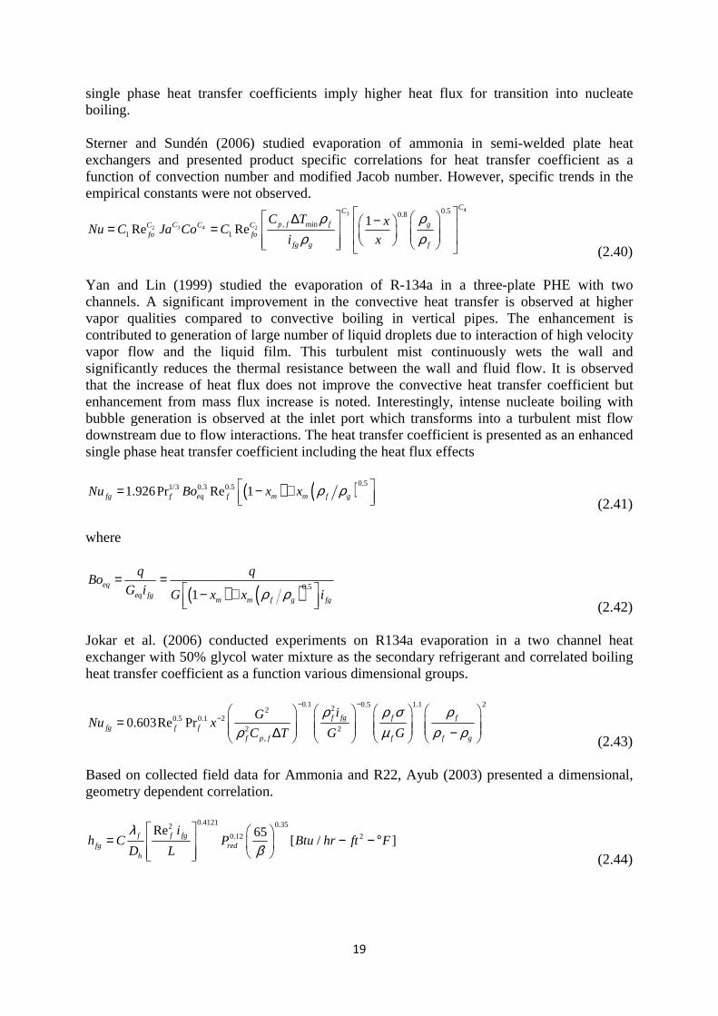
19

single phase heat transfer coefficients imply higher heat flux for transition into nucleate boiling. Sterner and Sundén (2006) studied evaporation of ammonia in semi-welded plate heat exchangers and presented product specific correlations for heat transfer coefficient as a function of convection number and modified Jacob number. However, specific trends in the empirical constants were not observed.

43

32 4 2

0.50.8, min

1 1

1Re Re

CC

p f f gCC C Cfo fo

fg g f

C T xNu C Ja Co C

i x

ρ ρρ ρ

∆ − = = (2.40)

Yan and Lin (1999) studied the evaporation of R-134a in a three-plate PHE with two channels. A significant improvement in the convective heat transfer is observed at higher vapor qualities compared to convective boiling in vertical pipes. The enhancement is contributed to generation of large number of liquid droplets due to interaction of high velocity vapor flow and the liquid film. This turbulent mist continuously wets the wall and significantly reduces the thermal resistance between the wall and fluid flow. It is observed that the increase of heat flux does not improve the convective heat transfer coefficient but enhancement from mass flux increase is noted. Interestingly, intense nucleate boiling with bubble generation is observed at the inlet port which transforms into a turbulent mist flow downstream due to flow interactions. The heat transfer coefficient is presented as an enhanced single phase heat transfer coefficient including the heat flux effects

( ) ( )0.51/3 0.3 0.51.926Pr Re 1fg f eq f m m f gNu Bo x x ρ ρ = − + (2.41)

where

( ) ( )0.51

eqeq fg

m m f g fg

q qBo

G i G x x iρ ρ= =

− + (2.42)

Jokar et al. (2006) conducted experiments on R134a evaporation in a two channel heat exchanger with 50% glycol water mixture as the secondary refrigerant and correlated boiling heat transfer coefficient as a function various dimensional groups.

0.1 1.1 20.5220.5 0.1 2

2 2,

0.603Re Pr f fg f ffg f f

f p f f f g

iGNu x

C T G G

ρ ρ σ ρρ µ ρ ρ

− −

−

= ∆ − (2.43)

Based on collected field data for Ammonia and R22, Ayub (2003) presented a dimensional, geometry dependent correlation.

0.4121 0.3520.12 2Re 65

[ / ]f f fgfg red

h

ih C P Btu hr ft F

D L

λβ

= − − °

(2.44)

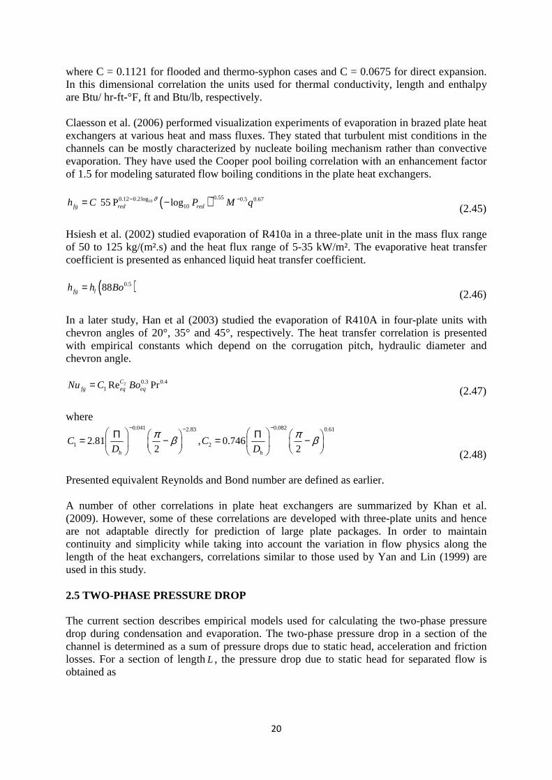
20

where C = 0.1121 for flooded and thermo-syphon cases and C = 0.0675 for direct expansion. In this dimensional correlation the units used for thermal conductivity, length and enthalpy are Btu/ hr-ft-°F, ft and Btu/lb, respectively. Claesson et al. (2006) performed visualization experiments of evaporation in brazed plate heat exchangers at various heat and mass fluxes. They stated that turbulent mist conditions in the channels can be mostly characterized by nucleate boiling mechanism rather than convective evaporation. They have used the Cooper pool boiling correlation with an enhancement factor of 1.5 for modeling saturated flow boiling conditions in the plate heat exchangers.

( )100.550.12 0.2log 0.5 0.67

1055 P logfg red redh C P M qϑ −− −= − (2.45)

Hsiesh et al. (2002) studied evaporation of R410a in a three-plate unit in the mass flux range of 50 to 125 kg/(m².s) and the heat flux range of 5-35 kW/m². The evaporative heat transfer coefficient is presented as enhanced liquid heat transfer coefficient.

( )0.588fg lh h Bo= (2.46)

In a later study, Han et al (2003) studied the evaporation of R410A in four-plate units with chevron angles of 20°, 35° and 45°, respectively. The heat transfer correlation is presented with empirical constants which depend on the corrugation pitch, hydraulic diameter and chevron angle.

2 0.3 0.41 Re PrC

fg eq eqNu C Bo= (2.47)

where

0.041 0.0822.83 0.61

1 22.81 , 0.7462 2h h

C CD D

π πβ β− −−

Π Π = − = − (2.48)

Presented equivalent Reynolds and Bond number are defined as earlier. A number of other correlations in plate heat exchangers are summarized by Khan et al. (2009). However, some of these correlations are developed with three-plate units and hence are not adaptable directly for prediction of large plate packages. In order to maintain continuity and simplicity while taking into account the variation in flow physics along the length of the heat exchangers, correlations similar to those used by Yan and Lin (1999) are used in this study. 2.5 TWO-PHASE PRESSURE DROP The current section describes empirical models used for calculating the two-phase pressure drop during condensation and evaporation. The two-phase pressure drop in a section of the channel is determined as a sum of pressure drops due to static head, acceleration and friction losses. For a section of lengthL , the pressure drop due to static head for separated flow is obtained as

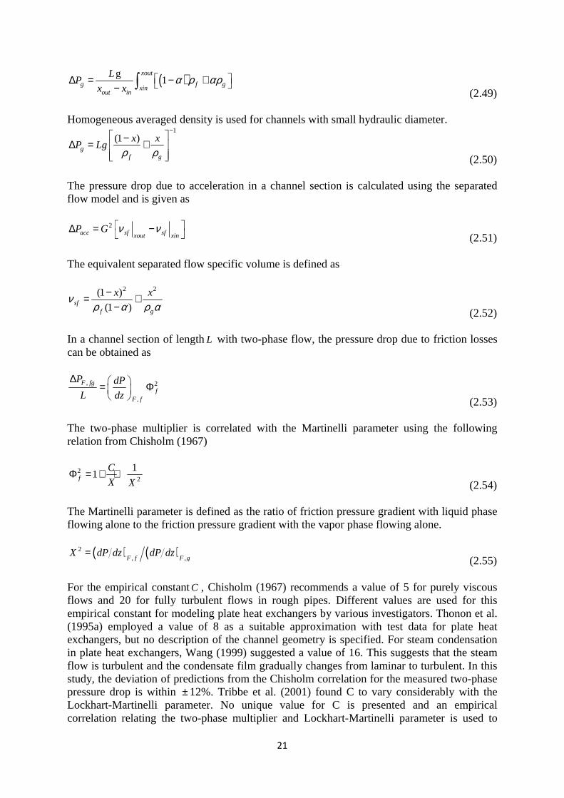
21

( )g1

xout

g f gxin

out in

LP

x xα ρ αρ ∆ = − + − ∫

(2.49)

Homogeneous averaged density is used for channels with small hydraulic diameter.

1(1 )

gf g

x xP Lg

ρ ρ

− −∆ = + (2.50)

The pressure drop due to acceleration in a channel section is calculated using the separated flow model and is given as

2acc sf sfxout xin

P G ν ν ∆ = − (2.51)

The equivalent separated flow specific volume is defined as

2 2(1 )

(1 )sff g

x xνρ α ρ α

−= +− (2.52)

In a channel section of lengthL with two-phase flow, the pressure drop due to friction losses can be obtained as

, 2

,

F fgf

F f

P dP

L dz

∆ = Φ (2.53)

The two-phase multiplier is correlated with the Martinelli parameter using the following relation from Chisholm (1967)

22

11f

C

X XΦ = + +

(2.54) The Martinelli parameter is defined as the ratio of friction pressure gradient with liquid phase flowing alone to the friction pressure gradient with the vapor phase flowing alone.

( ) ( )2, ,F f F g

X dP dz dP dz= (2.55)

For the empirical constantC , Chisholm (1967) recommends a value of 5 for purely viscous flows and 20 for fully turbulent flows in rough pipes. Different values are used for this empirical constant for modeling plate heat exchangers by various investigators. Thonon et al. (1995a) employed a value of 8 as a suitable approximation with test data for plate heat exchangers, but no description of the channel geometry is specified. For steam condensation in plate heat exchangers, Wang (1999) suggested a value of 16. This suggests that the steam flow is turbulent and the condensate film gradually changes from laminar to turbulent. In this study, the deviation of predictions from the Chisholm correlation for the measured two-phase pressure drop is within ± 12%. Tribbe et al. (2001) found C to vary considerably with the Lockhart-Martinelli parameter. No unique value for C is presented and an empirical correlation relating the two-phase multiplier and Lockhart-Martinelli parameter is used to

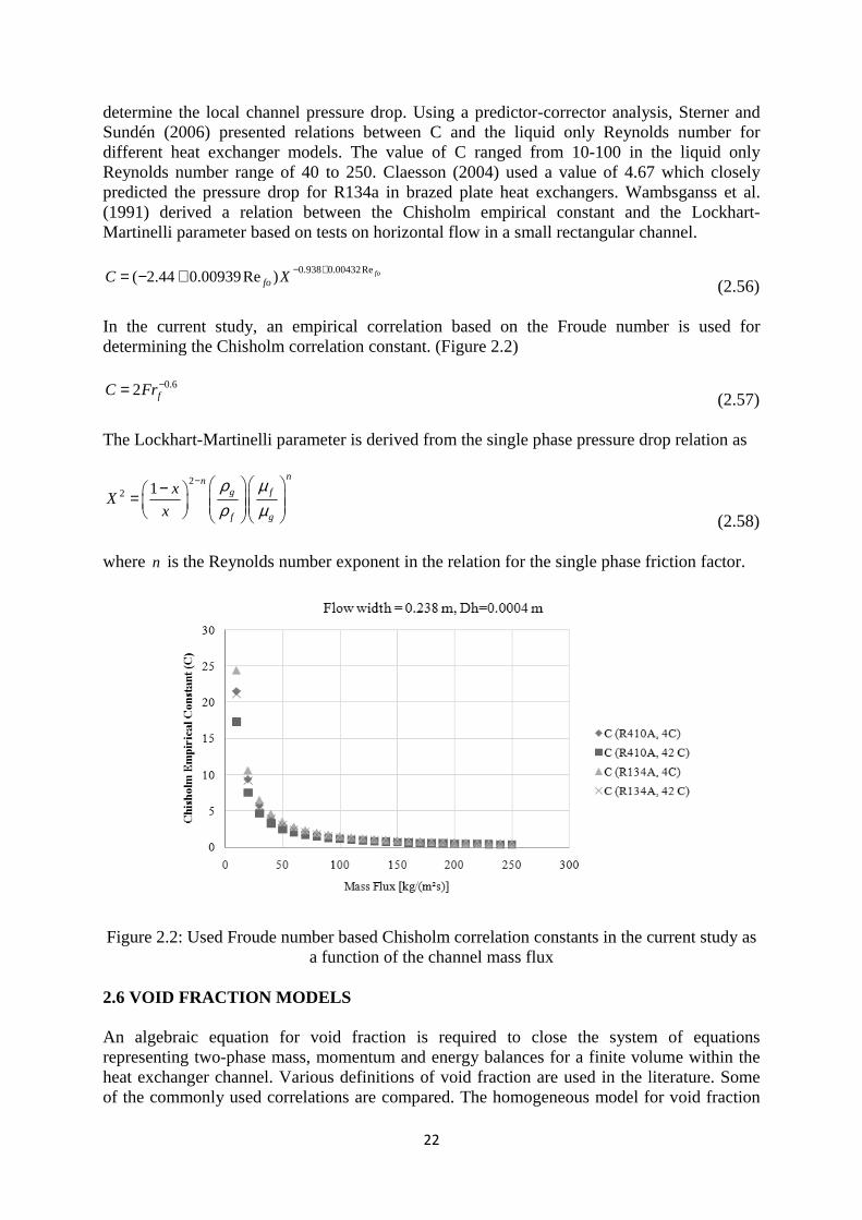
determine the local channel preSundén (2006) presented relations between C and the liquid only Reynolds number for different heat exchanger models. The value of C ranged from 10Reynolds number range ofpredicted the pressure drop for R134a in brazed plate heat exchangers. Wambsganss et al. (1991) derived a relation between the Chisholm empirical constant and the LockhartMartinelli parameter

( 2.44 0.00939Re )C X= − +

In the current study, an empirical correlation based on the Froude number is used for determining the Chisholm correlation constant.

0.62 fC Fr−=

The Lockhart-Martinelli parameter is derived from the single phase pressure drop relation as

22 1

nx

Xx

− − =

where n is the Reynolds number exponent in the relation for the single phase friction factor.

Figure 2.2: Used Froude number based Chisholm correlation constants in the current study as

2.6 VOID FRACTION MODELS An algebraic equation for void fraction is required to close the system of equations representing twoheat exchanger channel. Various definitions of void fraction are used in the literof the commonly used correlations are compared. The homogeneous model for void fraction

22

determine the local channel pressure drop. Using a predictorSundén (2006) presented relations between C and the liquid only Reynolds number for different heat exchanger models. The value of C ranged from 10Reynolds number range of 40 to 250. Claesson (2004) used a value of 4.67 which closely predicted the pressure drop for R134a in brazed plate heat exchangers. Wambsganss et al. (1991) derived a relation between the Chisholm empirical constant and the LockhartMartinelli parameter based on tests on horizontal flow in a small rectangular channel.

0.938 0.00432Re( 2.44 0.00939Re ) fo

foC X− +

In the current study, an empirical correlation based on the Froude number is used for determining the Chisholm correlation constant.

Martinelli parameter is derived from the single phase pressure drop relation as

n

g f

f g

ρ µρ µ

is the Reynolds number exponent in the relation for the single phase friction factor.

Figure 2.2: Used Froude number based Chisholm correlation constants in the current study as a function of the channel mass flux

2.6 VOID FRACTION MODELS

An algebraic equation for void fraction is required to close the system of equations representing two-phase mass, momentum and energy balances for a finite volume within the heat exchanger channel. Various definitions of void fraction are used in the literof the commonly used correlations are compared. The homogeneous model for void fraction

22

ssure drop. Using a predictor-corrector analysis, Sterner and Sundén (2006) presented relations between C and the liquid only Reynolds number for different heat exchanger models. The value of C ranged from 10-100 in the liquid only

40 to 250. Claesson (2004) used a value of 4.67 which closely predicted the pressure drop for R134a in brazed plate heat exchangers. Wambsganss et al. (1991) derived a relation between the Chisholm empirical constant and the Lockhart

based on tests on horizontal flow in a small rectangular channel.

In the current study, an empirical correlation based on the Froude number is used for (Figure 2.2)

Martinelli parameter is derived from the single phase pressure drop relation as

is the Reynolds number exponent in the relation for the single phase friction factor.

Figure 2.2: Used Froude number based Chisholm correlation constants in the current study as a function of the channel mass flux

An algebraic equation for void fraction is required to close the system of equations phase mass, momentum and energy balances for a finite volume within the

heat exchanger channel. Various definitions of void fraction are used in the literof the commonly used correlations are compared. The homogeneous model for void fraction

corrector analysis, Sterner and Sundén (2006) presented relations between C and the liquid only Reynolds number for

100 in the liquid only 40 to 250. Claesson (2004) used a value of 4.67 which closely

predicted the pressure drop for R134a in brazed plate heat exchangers. Wambsganss et al. (1991) derived a relation between the Chisholm empirical constant and the Lockhart-

based on tests on horizontal flow in a small rectangular channel.

(2.56)

In the current study, an empirical correlation based on the Froude number is used for

(2.57)

Martinelli parameter is derived from the single phase pressure drop relation as

(2.58)

is the Reynolds number exponent in the relation for the single phase friction factor.

Figure 2.2: Used Froude number based Chisholm correlation constants in the current study as

An algebraic equation for void fraction is required to close the system of equations phase mass, momentum and energy balances for a finite volume within the

heat exchanger channel. Various definitions of void fraction are used in the literature. Some of the commonly used correlations are compared. The homogeneous model for void fraction

23

assumes that the two phases flow at the same velocity. Hence the relation between the vapor quality and void fraction can be directly derived as

1 11 g

hg f

x

x

ρα ρ

− = + (2.59) Wang et al. (1999) used the correlations estimated for steam by Zivi (1964)

2/31 1

1 g

steam f

x

x

ρα ρ

− = + (2.60)

The slip ratio correlation approach assumes that the two phases are separated and flow at different velocities. The ratio of gas velocity to liquid velocity is thereby defined as the slip ratio. The void fraction then takes the following form including the influence of inter-phase slip.

1 11 g

sr f

xs

x

ρα ρ

− = + (2.61)

where the slip ratio s is defined as

g

f

us

u=

(2.62)

The slip ratio is calculated differently by various investigators. Corberán et al. (2005) have used the correlation proposed by Chisholm (1983) in modeling compact evaporators and condensers.

1/2

1 1 f

g

S xρρ

= − −

(2.63)

Some models use the Lockhart-Martinelli correlating parameter for defining the void fraction instead of modifying the homogeneous model. The Lockhart-Martinelli parameter for two-phase flow in rough tubes is derived as

0.50.91 g

ttf

xX

x

ρρ − = (2.64)

Wallis (1969) and Domanski et al. (1983) derived empirical correlations based on data presented by Lockhart-Martinelli on two-phase pressure drop.

( ) 0.3780.8

1

101100.823 0.157ln

ttttXtt

tttt

for XX

for XXα

− ≤+= > − (2.65)

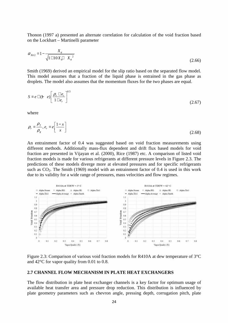
24

Thonon (1997 a) presented an alternate correlation for calculation of the void fraction based on the Lockhart – Martinelli parameter

2 21

1 10

ttXtt

tt tt

X

X Xα = −

+ + (2.66)

Smith (1969) derived an empirical model for the slip ratio based on the separated flow model. This model assumes that a fraction of the liquid phase is entrained in the gas phase as droplets. The model also assumes that the momentum fluxes for the two phases are equal.

0.5

(1 )1

r r

r

eS e e

e

ρ += + − + (2.67) where

1,f

r rg

xe e

x

ρρ

ρ− = =

(2.68) An entrainment factor of 0.4 was suggested based on void fraction measurements using different methods. Additionally mass-flux dependent and drift flux based models for void fraction are presented in Vijayan et al. (2000), Rice (1987) etc. A comparison of listed void fraction models is made for various refrigerants at different pressure levels in Figure 2.3. The predictions of these models diverge more at elevated pressures and for specific refrigerants such as CO2. The Smith (1969) model with an entrainment factor of 0.4 is used in this work due to its validity for a wide range of pressures, mass velocities and flow regimes.

Figure 2.3: Comparison of various void fraction models for R410A at dew temperature of 3°C and 42°C for vapor quality from 0.01 to 0.8. 2.7 CHANNEL FLOW MECHANISM IN PLATE HEAT EXCHANGERS The flow distribution in plate heat exchanger channels is a key factor for optimum usage of available heat transfer area and pressure drop reduction. This distribution is influenced by plate geometry parameters such as chevron angle, pressing depth, corrugation pitch, plate

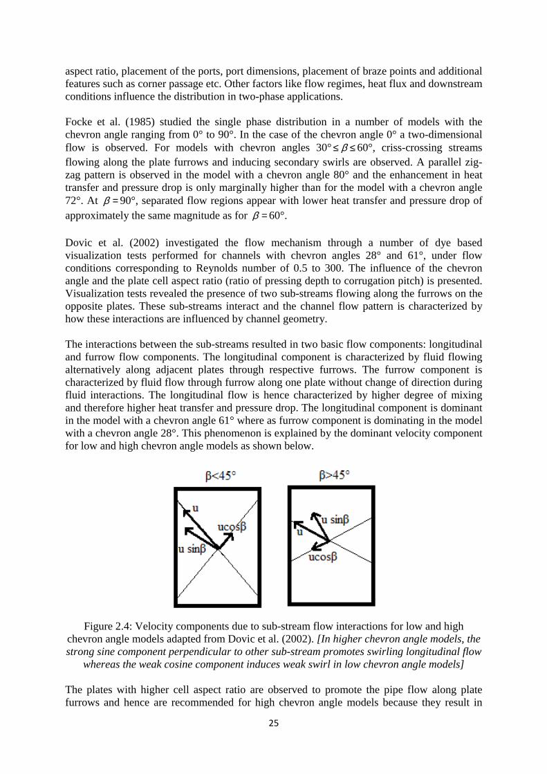
25

aspect ratio, placement of the ports, port dimensions, placement of braze points and additional features such as corner passage etc. Other factors like flow regimes, heat flux and downstream conditions influence the distribution in two-phase applications. Focke et al. (1985) studied the single phase distribution in a number of models with the chevron angle ranging from 0° to 90°. In the case of the chevron angle 0° a two-dimensional flow is observed. For models with chevron angles 30° β≤ ≤ 60°, criss-crossing streams flowing along the plate furrows and inducing secondary swirls are observed. A parallel zig-zag pattern is observed in the model with a chevron angle 80° and the enhancement in heat transfer and pressure drop is only marginally higher than for the model with a chevron angle 72°. At β = 90°, separated flow regions appear with lower heat transfer and pressure drop of approximately the same magnitude as for β = 60°. Dovic et al. (2002) investigated the flow mechanism through a number of dye based visualization tests performed for channels with chevron angles 28° and 61°, under flow conditions corresponding to Reynolds number of 0.5 to 300. The influence of the chevron angle and the plate cell aspect ratio (ratio of pressing depth to corrugation pitch) is presented. Visualization tests revealed the presence of two sub-streams flowing along the furrows on the opposite plates. These sub-streams interact and the channel flow pattern is characterized by how these interactions are influenced by channel geometry. The interactions between the sub-streams resulted in two basic flow components: longitudinal and furrow flow components. The longitudinal component is characterized by fluid flowing alternatively along adjacent plates through respective furrows. The furrow component is characterized by fluid flow through furrow along one plate without change of direction during fluid interactions. The longitudinal flow is hence characterized by higher degree of mixing and therefore higher heat transfer and pressure drop. The longitudinal component is dominant in the model with a chevron angle 61° where as furrow component is dominating in the model with a chevron angle 28°. This phenomenon is explained by the dominant velocity component for low and high chevron angle models as shown below.

Figure 2.4: Velocity components due to sub-stream flow interactions for low and high

chevron angle models adapted from Dovic et al. (2002). [In higher chevron angle models, the strong sine component perpendicular to other sub-stream promotes swirling longitudinal flow

whereas the weak cosine component induces weak swirl in low chevron angle models] The plates with higher cell aspect ratio are observed to promote the pipe flow along plate furrows and hence are recommended for high chevron angle models because they result in

26

more sub-stream interaction. Similarly, lower cell aspect ratio is recommended for low chevron angle models in-order to improve the longitudinal flow component. In studies performed on corrugated plates for identifying transition from nucleate boiling to convective boiling, Thonon (1997 b) observed that the convective mechanism dominates at low wall to fluid temperature difference and nucleation dominates at higher temperature differences. For a corrugated channel, the product of boiling number and Lockhart-Martinelli

parameter is used as a transition number. If the flow conditions imply( )3. 0.15 10Bo X −> × , the

heat transfer coefficient depends on nucleate boiling. Yin (1999) suggested that great increase of vapor volume during the evaporation process causes the vapor flow to move at a greater speed which breaks the adjacent fluid film into tiny liquid droplets. This characteristic flow is termed as high speed turbulent mist flow and results in great reduction of thermal resistance due to continuous wetting of the heat transfer area at the wall. In contrast, Claesson et al. (2006) suggest that thin film evaporation is the dominant heat transfer mechanism. Visualization experiments are conducted using temperature sensitive paints to determine the heat flux and heat transfer coefficient based on the wetted area. Results are presented and the heat transfer coefficient was found to correlate well to the heat flux and not at all to the mass flux. As this type of evaporation is common during nucleate boiling, the authors suggested to use of enhanced pool boiling correlations for evaporation in plate heat exchangers. Shiomi et al. (2004) conducted visualization of adiabatic gas-liquid flow in Plexiglas corrugated plates sections in horizontal and vertical conditions. Channels with mixed chevron angle combinations from 30° and 60° plates were tested. In horizontal flow tests, the gas-liquid phases are separated completely at low liquid flux. With increase of liquid flux, bubbles were distributed uniformly over the plate. Referring to standard flow regime maps, it is suggested that the stratified flow exist at higher liquid fluxes compared to circular tubes. The corrugation angle of the upper plate is found to strongly affect the flow pattern and pressure drop at horizontal condition. Only dispersed flow is observed in vertical flow. When the gas flux is small, the bubbles were moved to one side of the plate. The bubble distribution is observed to be more uniform with increasing gas flux. The bubble diameters at the outlet section were smaller compared to the inlet due to fragmentation but were found to be more uniform with increasing liquid flux. Tribbe et al. (2001) studied the flow patterns in single phase flow and adiabatic gas-liquid flows in plate and frame heat exchangers. The test section was prepared from transparent polyester plates and was fixed by special pressure plates with observation ports. Crossing and longitudinal flow were observed in single phase mode as presented in a number of studies. The single phase flow mechanism at the spine of the chevron pattern was also studied. In non-mixing channels, the spine acts as a physical boundary and hence the flow approaching the spine is reflected and directed along the furrows on the opposite plate. In channels formed with mixed plates, the phase shift between the plates is variable. When in phase, a channel is formed along the spine and allows fluid flow and when the corrugations become out of phase, the fluid flows along the furrows on both sides of the spine. In gas-liquid flow, flow patterns such as regular bubble flow, irregular bubble flow, churn flow, film flow and partial film flow are identified. Flow pattern maps for this adiabatic flow are presented using liquid and gas velocities as parameters. The understanding of the flow mechanism while using plates with various geometry parameters, the relationship between the observed flow patterns and the thermal and hydraulic

27

performance of the heat exchanger, influence of heat exchanger orientation on channel flow mechanism etc., provide a value input for development of appropriate thermal and hydraulic correlations which include these effects. Such correlations provide a more reliable base for the prediction of performance with new plate patterns, flow arrangements and while using alternative refrigerants. 2.8 INFLUENCE OF FLUID PROPERTIES ON BPHE PERFORMANCE The choice of operating media for a specific application is governed by the factors such as the thermodynamic and transport properties of the fluid, compatibility of the fluid with the BPHE materials, operating pressures, local legislations etc. The understanding of the relation between the physical properties of the fluid and the heat exchanger performance helps in the prediction and design of plate heat exchangers for alternate refrigerants and applications. The single phase pressure drop in plate heat exchangers is mainly dependent on the viscosity and density of the fluid. The single phase pressure drop model used in this study reduces to

2 1np npP m µ ρ− −∆ ∝ ɺ (2.69) The exponent ‘np’ usually ranges from 0 to 0.3 for Re>100 and from 0.2 to 1.2 for Re<100. This empirical constant is a function of the plate geometry parameters such as the chevron angle, corrugation pitch etc. The single phase heat transfer relation (Equation 2.9) reduces to the following relation

1nh y y y nhph m C λ µ− −∝ ɺ (2.70)

The Prandtl number exponent ‘y’ value is around 0.4 for commonly used fluids (for both pure liquid and gas phases) within normal operating temperatures and pressures. The value of ‘nh’ ranges from 0.6 to 0.8 for fully turbulent flow and is a function of the plate geometry parameters. As a rule of thumb, for turbulent flow, one can assume 0, 0.7 and 0.4 for the values of np, nh and y, respectively, which gives the relation between the heat exchanger goodness and fluid properties at a given flow rate.

0.6 0.4

0.3

pCh

P

ρ λµ

∝∆

(2.71)

The choice of refrigerant influences the performance of the heat exchanger and the refrigeration system. Factors such as miscibility of the selected lubrication oil with the used refrigerant influence the degree of fouling. Poor oil carry over in heat exchanger channels and lack of efficient oil separation devices would result in accumulation of oil pools in heat exchanger ports and channels resulting in bad distribution and control issues due to unstable performance of heat exchanger. Usually, the refrigerants with low molecular weight are associated with lower mass flow rates and hence, lower pressure drops. Critical temperatures also tend to be high for low molecular weight fluids. Operating conditions such as higher condensing pressures (closer to critical

28

point) reduces efficiency due to lower latent heat of evaporation. Lower viscosity and high thermal conductivity are also desirable in case of two-phase flows. Surface tension and the slope of the pressure/temperature curve are the measure of the ease with which a refrigerant can be induced to boil. (Forbes 2008). The amount of saturation temperature loss for unit pressure drop is an important factor in design of heat exchangers for refrigeration applications. This factor limits the heat transfer due to internal temperature pinch points. Hence, the pressure temperature relationship and heat transfer coefficient should be considered together in the design of heat exchangers. Other refrigerant properties such as the ratio of latent heat to specific volume of vapor, ratio of specific heats, specific volume of vapor at suction condition, critical temperature etc have significant influence on the size and efficiency of the refrigeration system. REFERENCES Ayub, Z. H., Plate Heat Exchanger Literature Survey and New Heat Transfer and Pressure Drop Correlations for Refrigerant Evaporators, Heat Transfer Engineering, 24(5), pp. 3-16, 2003. Bogaert, R., Brazed Plate Heat Exchanger Project, Part 2: Thermal Characteristics of the Brazed Plate Heat Exchanger, Report LTT-94-06, Ecole Polytechnique Federale De Lausanne, 1994 Boyko, L., and Kruzhilin, G., Heat Transfer and Hydraulic Resistance during Condensation of Steam in an Horizontal Tube and in Bundles of Tubes, International Journal of Heat and Mass Transfer, Volume 10, pp. 361-373, 1967 Chisholm, D., A Theoretical Basis for the Lockhart-Martinelli Correlation for Two-Phase Flow, International Journal of Heat and Mass Transfer, Volume 10, pp. 1767-1778, 1967. Chen, J. C., A Correlation for Boiling Heat Transfer to Saturated Fluids in Convective Flow, ASME preprint 63-HT-34, 6th National Heat Transfer Conference, Boston, 1963. Chisholm, D., Two Phase Flow in Pipelines and Heat Exchangers, George Godwin, London and New York, 1983. Claesson, J., Thermal and Hydraulic Performance of Compact Brazed Plate Heat Exchangers Operating as Evaporators in Domestic Heat Pumps, PhD thesis, Dept. of Energy Technology, Royal Institute of Technology, Sweden, ISBN 91-7283-931-7, 2004. Palm, B., and Claesson, J., Plate Heat Exchangers: Calculation Methods for Single and Two-Phase Flow, Heat Transfer Engineering, 27 (4), pp. 88-98, 2006. Collier, J.G., and Thome, J.R., Convective Boiling and Condensation, 3rd edition, Oxford University Press Inc., New York, 1999. Cooper, A., Condensation of Steam in Plate Heat Exchangers, AIChE Symp. 70 (138): pp. 172-177, 1987.

29

Corberán, J.M., Urchueguia, J., and Gonzálvez, J., Two Phase Heat Transfer in Brazed Plate Heat Exchangers, Evaporators and Condensers for R22 and Propane, Proceedings of Eurotherm 2000, 2000. Domanski, P., and Didion, D., Computer Modeling of the Vapor Compression Cycle with Constant Flow Area Expansion Device, NBS Building Science Series 155, 1983. Dovic, D., Palm. B., and Svaic, S., Basic Single-Phase Flow Phenomena in Chevron-Type Plate Heat Exchangers, Zero Leakage – Minimum Charge, IIR/IIF, Stockholm, pp. 221-232, 2002. Focke, W. W., Zachariades, J., and Olivier, I., The Effect of the Corrugation Inclination Angle on the Thermohydraulic Performance of Plate Heat Exchangers, International Journal of Heat and Mass Transfer, Volume 28, No 8, pp. 1469-1479, 1985. Forbes, P.S., Saving Energy in Refrigeration, Air-Conditioning and Heat-Pump Technologies, 2nd Edition, International Institute of Refrigeration, pp. 45-50, 2008. Gullapalli, V.S., Condensation in Compact Brazed Plate Heat Exchangers: Evaluation and Performance Analysis, Heat Set 2007 – Heat Transfer in Components and Systems for Sustainable Energy Technologies, Chambery, France, 2007. Han, D., Lee, K., and Kim, Y., Experiments on the Characteristics of Evaporation of R410A in Brazed Plate Heat Exchangers with Different Geometric Configurations, Applied Thermal Engineering 23 (2003) pp. 1209-1225, 2003. Heavner, R.L., Kumar, H., and Wanniarachchi, A.S., Performance of Industrial Plate Heat Exchanger: Effect of Chevron Angle, AIChE Symposium Series, Heat Transfer – Atlanta 1993, Volume 89, No 295, pp. 262-267, 1993. Hsieh, Y.Y. and Lin, T.F., Saturated Flow Boiling Heat Transfer and Pressure Drop of Refrigerant R-410a in a Vertical Plate Heat Exchanger, International Journal of Heat and Mass Transfer, Volume 45, pp. 1033-1044, 2002. Incropera, F. P., and DeWitt, D.P., Fundamentals of Heat and Mass Transfer, John Wiley & Sons, Inc, Chapter 11: Heat Exchangers, pp. 658-666, 1990. Jokar, A., Hosni, M.H., and Eckels, S.J., Dimensional Analysis on the Evaporation and Condensation of Refrigerant R-134a in Mini Channel Plate Heat Exchangers, Applied thermal engineering 26 (2006), pp. 2287-2300, 2006. Khan, T.S., Khan, M.S., Chyu, M., Ayub, Z.H., and Javed, A., Review of Heat Transfer and Pressure Drop Correlations for Evaporation and Fluid Flow in Plate Heat Exchangers, HVAC & R Research, Volume 15, No 2, pp. 169-188, 2009. Kuo, W. S., Lie, Y.M., Hsieh, Y.Y., and Lin, T.F., Condensation Heat Transfer and Pressure Drop of Refrigerant R-410A Flow in a Vertical Plate Heat Exchanger, International Journal of Heat and Mass Transfer 48 (2005), pp. 5205-5220, 2005.

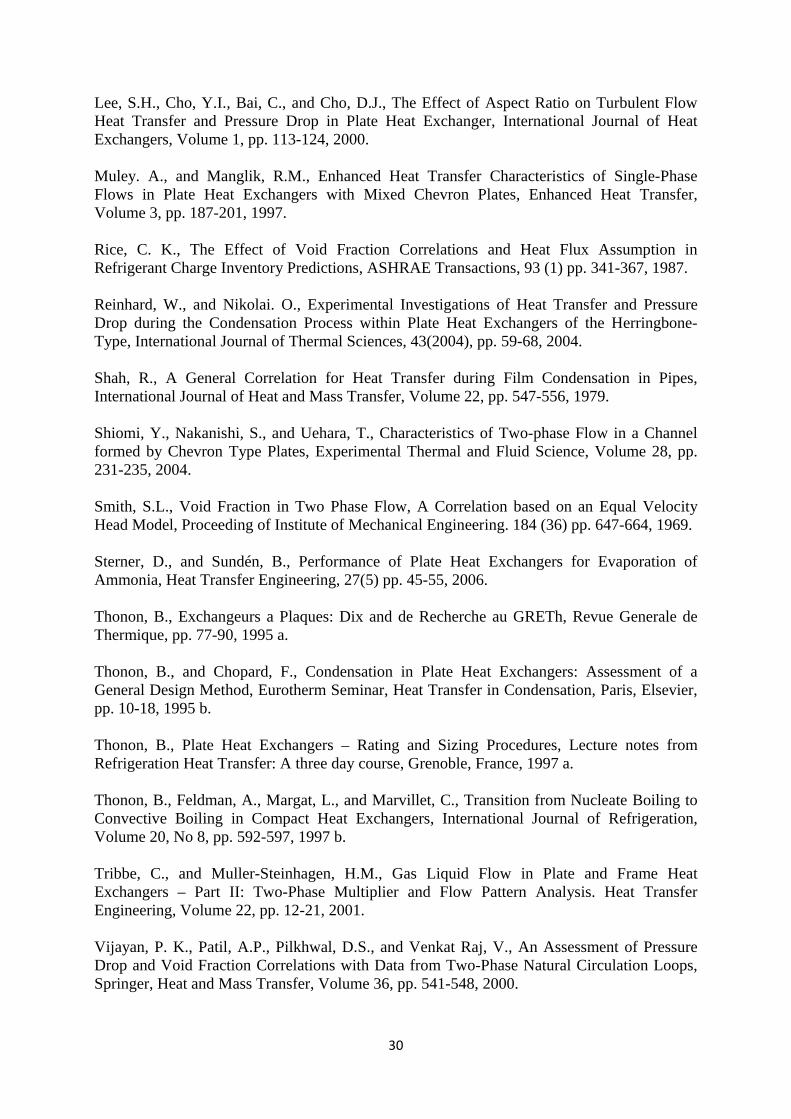
30

Lee, S.H., Cho, Y.I., Bai, C., and Cho, D.J., The Effect of Aspect Ratio on Turbulent Flow Heat Transfer and Pressure Drop in Plate Heat Exchanger, International Journal of Heat Exchangers, Volume 1, pp. 113-124, 2000. Muley. A., and Manglik, R.M., Enhanced Heat Transfer Characteristics of Single-Phase Flows in Plate Heat Exchangers with Mixed Chevron Plates, Enhanced Heat Transfer, Volume 3, pp. 187-201, 1997. Rice, C. K., The Effect of Void Fraction Correlations and Heat Flux Assumption in Refrigerant Charge Inventory Predictions, ASHRAE Transactions, 93 (1) pp. 341-367, 1987. Reinhard, W., and Nikolai. O., Experimental Investigations of Heat Transfer and Pressure Drop during the Condensation Process within Plate Heat Exchangers of the Herringbone-Type, International Journal of Thermal Sciences, 43(2004), pp. 59-68, 2004. Shah, R., A General Correlation for Heat Transfer during Film Condensation in Pipes, International Journal of Heat and Mass Transfer, Volume 22, pp. 547-556, 1979. Shiomi, Y., Nakanishi, S., and Uehara, T., Characteristics of Two-phase Flow in a Channel formed by Chevron Type Plates, Experimental Thermal and Fluid Science, Volume 28, pp. 231-235, 2004. Smith, S.L., Void Fraction in Two Phase Flow, A Correlation based on an Equal Velocity Head Model, Proceeding of Institute of Mechanical Engineering. 184 (36) pp. 647-664, 1969. Sterner, D., and Sundén, B., Performance of Plate Heat Exchangers for Evaporation of Ammonia, Heat Transfer Engineering, 27(5) pp. 45-55, 2006. Thonon, B., Exchangeurs a Plaques: Dix and de Recherche au GRETh, Revue Generale de Thermique, pp. 77-90, 1995 a. Thonon, B., and Chopard, F., Condensation in Plate Heat Exchangers: Assessment of a General Design Method, Eurotherm Seminar, Heat Transfer in Condensation, Paris, Elsevier, pp. 10-18, 1995 b. Thonon, B., Plate Heat Exchangers – Rating and Sizing Procedures, Lecture notes from Refrigeration Heat Transfer: A three day course, Grenoble, France, 1997 a. Thonon, B., Feldman, A., Margat, L., and Marvillet, C., Transition from Nucleate Boiling to Convective Boiling in Compact Heat Exchangers, International Journal of Refrigeration, Volume 20, No 8, pp. 592-597, 1997 b. Tribbe, C., and Muller-Steinhagen, H.M., Gas Liquid Flow in Plate and Frame Heat Exchangers – Part II: Two-Phase Multiplier and Flow Pattern Analysis. Heat Transfer Engineering, Volume 22, pp. 12-21, 2001. Vijayan, P. K., Patil, A.P., Pilkhwal, D.S., and Venkat Raj, V., An Assessment of Pressure Drop and Void Fraction Correlations with Data from Two-Phase Natural Circulation Loops, Springer, Heat and Mass Transfer, Volume 36, pp. 541-548, 2000.

31

Nakaoka, T., and Uheara, H, Performance Test of a Shell and Plate Type Condenser for OTEC, Experimental Thermal and Fluid science, Volume 1, pp. 275-281, 1998. Wallis, G.B., One-Dimensional Two-Phase Flow, New York: McGraw-Hill, pp. 51-54, 1969. Wambsganss, M.W., Jendrzejczyk, J.A., and France, D.M., Two-Phase Flow Patterns and Transitions in Small, Horizontal, Rectangular Channel, International Journal of Multiphase Flow, 17(3), pp. 327-342, 1991. Wang, L., Christensen, R., and Sundén, B., Calculation Procedure for Steam Condensation in Plate Heat Exchangers, Compact Heat Exchangers and Enhancement Technology for the Process Industries, Begell House, pp. 479-484, 1999. Wang, L., Christensen, R., and Sundén, B., An Experimental Investigation of Steam Condensation in Plate Heat Exchangers, International Journal of Heat Exchangers, Volume 1 (2000), pp. 125-150, 2000. Wang, L., Sundén, B., and Manglik, R.M., Plate Heat Exchangers: Design, Applications and Performance, WIT Press, ISBN 978-1-85312-737-3, 2007. Yan Y., Lio, H., and Lin, T., Condensation Heat Transfer and Pressure Drop of Refrigerant R-134a in a Plate Heat Exchanger, International Journal of Heat and Mass Transfer 42(1999), pp. 993-1006, 1999. Yan, Y. Y., and Lin, T.F., Evaporation Heat Transfer and Pressure Drop of Refrigerant R-134a in a Plate Heat Exchanger, ASME Journal of Heat Transfer, Volume 121, No 1, pp. 118-127, 1999. Zivi, S.M., Estimation of Steady-State Steam Void Fraction by means of the Principle of Minimum Entropy Production, ASME Journal of Heat Transfer, 86(2) pp. 247-252, 1964.

32

3.0 DISCRETIZED CALCULATIONS

Discretized calculations are essential for better resolution of local conditions in heat exchanger calculations. Large variation of thermo-physical properties of fluids with respect to local temperature and pressure, internal temperature pinch points etc., introduce errors in lumped parameter approaches while calculating energy balance and area requirements. The current chapter discusses various discretization schemes available in the literature and the methods used in the current study. Pressure-enthalpy based generalized rating method developed in the present study is described in detail. Mesh interpolation methods developed for obtaining accurate and continuous fluid properties are also described. Optimization techniques used for parameter estimation in single phase, two-phase thermal and hydraulic correlations are briefly mentioned.

3.1 INTRODUCTION In the current study, a discretized, general and continuous rating calculation method is presented. The rating calculations are used to determine the suitability of a heat exchanger model for a given thermal and hydraulic requirement. The input parameters for these calculations include the heat exchanger geometry parameters, available heat transfer area, flow arrangement, heat transfer media, and thermal duty/pressure drop limitations. The rating calculations return the thermal suitability with a parameter termed as oversurface (ratio of area available to area required) and actual pressure drops expected for all fluid streams. 3.1.1 Desirable Features of Rating Method The following features are desirable characteristics of a heat exchanger rating method for implementation in commercial heat exchanger selection software and refrigeration system simulation applications. Accuracy and Scalability: Laboratory tests usually do not cover the entire operating envelope of a heat exchanger. The thermal and hydraulic performance observed for a model at a given heat flux varies with the size of the heat exchanger due to additional influences such as deterioration of flow distribution, changes in flow regimes etc. The developed rating method should be able to take a sufficient number of parameters into account so that the predictions will be accurate within a specified uncertainty in the entire operational envelope. General, Continuous and Robust: In order to facilitate integration with external simulation programs and other calculation modules, the developed rating method should be continuous. Iterative schemes such as Newton-Raphson method demand at least first order continuity. It is hence required to use continuous form of thermal and hydraulic correlations, functions of fluid properties etc in the rating method. The developed rating method is also required to be general (application independent) to promote the continuity. For example, a heat recovery application in chillers involves calculations on de-superheaters (heat recovery applications). Depending on the outlet conditions, the calculation can be a single phase calculation or a condenser calculation involving phase change. An application independent rating calculation

33

would facilitate continuity in such situations. Robustness is required when handling cases such as internal temperature pinches, calculating cases with largely varying fluid properties, strong pressure-temperature dependence etc. Extendable, Informative and Calibrating Possibility: The rating method should work together with parameter estimation routines for determining the empirical constants in thermal and hydraulic correlations. Usually a combination of a heat exchanger model, heat transfer media and flow arrangement acquire a set of unique empirical constants. These constants provide information such as relative improvement or deterioration of performance with respect to parameters such as geometric dimensions of the heat exchanger, refrigerant characteristics etc. Using this information, the rating model should be extendable to predict the performance while using virtual heat exchanger models and alternate heat transfer media. Warnings and Software Performance: Selection and performance calculations involve a large number of iterative rating calculations and hence the rating calculation model should be computationally inexpensive. Memory usage should be limited for online applications. Additionally, warnings and error messages should be thrown by the calculation methods in case of undesirable conditions such as crossing temperatures, excessive flow maldistribution, flow velocities that are out of recommended range, undesirable flow regimes etc. 3.2 SOME DISCRETIZED METHODS IN THE LITERATURE Several 1D and 2D discretization models have been presented in the literature for plate heat exchanger analysis, especially for the applications involving phase change and multi- component flows. Some of these are summarized here. 3.2.1 HTRI Method for Condenser Design A one-dimensional discretized model involving the segmentation of flow paths in shell-and-tube heat exchangers into equal heat load sections is presented in the HTRI design manual. For a segment ‘n’ , the area required or overall heat transfer coefficient required to fulfill the assigned capacity can be determined if the other parameter is known using the relation

[ ] 1

0

nQ

n n nU A T dQ−= ∆∫ (3.1)

The selection calculation involves the following steps:

- Estimate area required (nA ) using LMTD and an arbitrary overall heat transfer coefficient ( nU ).

- Based on the area requirement, choose the shell side and tube side geometry parameters.

- Determine the actual overall heat transfer coefficient ( nU ) based on the selected geometry, actual temperature profiles and local flow conditions. Iteratively adjust the geometry until the calculated area required (nA ) and the value calculated in previous iteration closely agree.

- Calculate the pressure drops and adjust the geometry parameters further based on the allowable pressure drop on each side.

34

3.2.2 Semi Explicit Method for Wall Temperature Linked Equations An explicit wall temperature linked model was presented for heat exchanger performance calculations by Corberán et al. (2000). The flow in the channels or pipes is approximated to be one-dimensional and discretized into an arbitrary number of segments. Using link of wall temperatures, the treatment of fluid flow on all the sides of the heat exchanger is de-coupled. The flow evolution along the length of the channel is determined by integration of one-dimensional conservative equations. For two-phase flow in the ‘z’ direction in each segment, the conservative equations are G uρ= (3.2)

( )22 2 22 22 1 (1 )

(1 ) sin(1 )f g f

h f g f

fG xdP d x xG g

dz D dzρ α ρ α θ

ρ ρ α ρ α − −

− = Φ + + + + − − (3.3)

( )2 2 2 2

2 2 2 2

(1 )(1 ) sin

2 2 (1 )g f w

g f

d G x G xAG x i x i zg h T T

dzθ

ρ α ρ α

− + + − + + = Θ − −

(3.4)

At the walls, the balance of the heat exchanged from the surrounding fluids and the longitudinal conduction in the wall is maintained.

2

1,2

10w side

n side

t T QA

λ=

∇ + =∑ (3.5)

The global solution strategy involves the following steps:

- A trial wall temperature distribution is guessed and the governing equations are explicitly solved to determine the outlet conditions in each cell from the specified inlet values.

- The wall temperature in every cell is then determined explicitly based on local energy balance using equation 3.5

- The procedure is repeated until convergence in wall temperature is achieved. 3.2.3 Incremental Procedure in Condenser Calculations Arman and Rabas (1995) presented an incremental procedure for calculation of condensation in binary mixtures. Wang et al. (1999) presented a similar method for design calculations of steam condensation in plate heat exchangers. The flow paths are discretized into a finite number of equal area segments. The incremental procedure involves the following steps:

- Guess the outlet pressures and quality on the refrigerant side for an increment ‘n’ - Calculate the outlet saturation temperature based on the guessed outlet pressure. Guess

a value for the outlet vapor quality. - Calculate the wall heat flux based on the condensation side energy balance - Determine the outlet temperature on the coolant side using the calculated wall heat

flux

- Using the determined inlet and outlet conditions, calculate new wall heat flux and overall heat transfer coefficient

- Iterate on the guessed vapor quality the wall heat flux determined from condenser side energy balance and wall heat flux calculated using overall heat transfer coefficient.

- Calculate the coolant and condensation side pressure drops for the segm- Iterate on the guessed pressure in step 1, until convergence is observed between the

guessed and calculated outlet pressures. Wang et al. (1999) used the iterative procedure for evaluation of condensation heat transfer correlations and empirical mod 3.2.4 Performance Analysis of BPHE: Full Flow Path Discretization A complete one-was presented by Gullapalli (2008). The flow path on each side represented by onethis model, various effects of thermal interaction of fluid streams due to different flow arrangements can be captured. Using implicit models,fluid properties on the distribution can also be studied. The developed model can be used for performance calculations where a few boundary conditions are not known.

Figure 3.1: Discretization scheme of fluid flow

Conservative equations (similar to equations 3.2 to 3.4) are solved for each element representing the flow path. Wall temperature equations are solved oenthalpy profiles are determined on both sides. The global system of equations can be solved explicitly with wall temperature link as presented by Corberán et al. (2000) or using a Newton Raphson based iterative implicit method. Dependmethods can be very demanding computationally but are more robust compared to explicit methods. It is also possible to determine the flow distribution into various channels using the mass flow – pressure drop couplinobtained in counter and coFigure 3.2. The developed model could not be implemented in selection software due calibration of condensation heat transfer correlations was presented by Gullapalli (2007)

35

Using the determined inlet and outlet conditions, calculate new wall heat flux and overall heat transfer coefficient Iterate on the guessed vapor quality in step 2, until convergence is achieved between the wall heat flux determined from condenser side energy balance and wall heat flux calculated using overall heat transfer coefficient.Calculate the coolant and condensation side pressure drops for the segmIterate on the guessed pressure in step 1, until convergence is observed between the guessed and calculated outlet pressures.

Wang et al. (1999) used the iterative procedure for evaluation of condensation heat transfer correlations and empirical model for two-phase pressure drop.

3.2.4 Performance Analysis of BPHE: Full Flow Path Discretization

-dimensional discretization model of fluid flow paths in plate heat exchangers was presented by Gullapalli (2008). The flow path on each side represented by one-dimensional elements extended between nodesthis model, various effects of thermal interaction of fluid streams due to different flow arrangements can be captured. Using implicit models,fluid properties on the distribution can also be studied. The developed model can be used for performance calculations where a few boundary conditions are not known.

Figure 3.1: Discretization scheme of fluid flow

pass, 25 plates BPHE model presented by Gullapalli (2008)

Conservative equations (similar to equations 3.2 to 3.4) are solved for each element representing the flow path. Wall temperature equations are solved oenthalpy profiles are determined on both sides. The global system of equations can be solved explicitly with wall temperature link as presented by Corberán et al. (2000) or using a Newton Raphson based iterative implicit method. Dependmethods can be very demanding computationally but are more robust compared to explicit methods. It is also possible to determine the flow distribution into various channels using the

pressure drop coupling in this model. Example of the temperature profiles obtained in counter and co-current flow in a single phase performance calculation is shown in

igure 3.2. The developed model could not be implemented in selection software due to the speed limitations. An extension of the developed model for calibration of condensation heat transfer correlations was presented by Gullapalli (2007)

35

Using the determined inlet and outlet conditions, calculate new wall heat flux and

in step 2, until convergence is achieved between the wall heat flux determined from condenser side energy balance and wall heat flux calculated using overall heat transfer coefficient. Calculate the coolant and condensation side pressure drops for the segmIterate on the guessed pressure in step 1, until convergence is observed between the

Wang et al. (1999) used the iterative procedure for evaluation of condensation heat transfer phase pressure drop.

3.2.4 Performance Analysis of BPHE: Full Flow Path Discretization

dimensional discretization model of fluid flow paths in plate heat exchangers was presented by Gullapalli (2008). The flow path on each side of the heat exchanger is

dimensional elements extended between nodes as show in Figure 3.1this model, various effects of thermal interaction of fluid streams due to different flow arrangements can be captured. Using implicit models, influence of geometry parameters and fluid properties on the distribution can also be studied. The developed model can be used for performance calculations where a few boundary conditions are not known.

Figure 3.1: Discretization scheme of fluid flow path in counter flow arrangement for a three

pass, 25 plates BPHE model presented by Gullapalli (2008)

Conservative equations (similar to equations 3.2 to 3.4) are solved for each element representing the flow path. Wall temperature equations are solved once the pressure and enthalpy profiles are determined on both sides. The global system of equations can be solved explicitly with wall temperature link as presented by Corberán et al. (2000) or using a Newton Raphson based iterative implicit method. Depending on the number of segments, implicit methods can be very demanding computationally but are more robust compared to explicit methods. It is also possible to determine the flow distribution into various channels using the

g in this model. Example of the temperature profiles current flow in a single phase performance calculation is shown in

igure 3.2. The developed model could not be implemented in commercial to the speed limitations. An extension of the developed model for

calibration of condensation heat transfer correlations was presented by Gullapalli (2007)

Using the determined inlet and outlet conditions, calculate new wall heat flux and

in step 2, until convergence is achieved between the wall heat flux determined from condenser side energy balance and wall heat flux

Calculate the coolant and condensation side pressure drops for the segment Iterate on the guessed pressure in step 1, until convergence is observed between the

Wang et al. (1999) used the iterative procedure for evaluation of condensation heat transfer

dimensional discretization model of fluid flow paths in plate heat exchangers of the heat exchanger is as show in Figure 3.1. In

this model, various effects of thermal interaction of fluid streams due to different flow influence of geometry parameters and

fluid properties on the distribution can also be studied. The developed model can be used for

path in counter flow arrangement for a three

Conservative equations (similar to equations 3.2 to 3.4) are solved for each element nce the pressure and

enthalpy profiles are determined on both sides. The global system of equations can be solved explicitly with wall temperature link as presented by Corberán et al. (2000) or using a Newton

ing on the number of segments, implicit methods can be very demanding computationally but are more robust compared to explicit methods. It is also possible to determine the flow distribution into various channels using the

g in this model. Example of the temperature profiles current flow in a single phase performance calculation is shown in

heat exchanger to the speed limitations. An extension of the developed model for

calibration of condensation heat transfer correlations was presented by Gullapalli (2007)

36

Figure 3.2: Temperature distribution in single phase flow in counter and co-current flow

arrangements obtained using the flow path discretization model in Gullapalli (2008) 3.2.5 Other Discretization Models Strelow (2000) presented a generalized calculation procedure for arbitrary number of flow passes and flow streams in a heat exchanger. Although discretization of the flow streams is not involved, the proposed model is very useful in multi-stream heat exchangers. Mayta Tito et al. (2011) presented a four zone model for a brazed plate cascaded condenser. The overall heat transfer coefficient in each zone was determined using lumped models without further discretization. Pacio et al. (2011) presented a one-dimensional stream evaluation model for two-phase applications in tube-in-tube heat exchangers. The conservation equations for each segment use the temperature difference on both sides rather than the bulk to wall temperature difference. Mancin et al. (2011) presented a pressure-temperature based one-dimensional model for vapor condensation of R410A. This model is very similar to the model proposed by Corberán et al. (2000) and can be used for rating calculations as well.

3.3 DEVELOPED GENERALIZED STEPWISE RATING SCHEME In the current study a discretized and continuous rating method is developed for implementation in SWEP software package SSPG7 (SWEP heat exchanger selection software). For ease of implementation and to generalize the calculation framework for all kind of applications, the model works in the pressure-enthalpy domain instead of the generally used pressure-temperature domain. A standard selection calculation in a commercial software would involve iterative use of the rating method. The calculation would iterate through hundreds of heat exchanger models in the product tree, various combinations of plates, parallel units, flow arrangements, number of passes etc., resulting in thousands of calls to the rating method. In order to guarantee selection of heat exchangers for a given thermal and hydraulic duty in a reasonable time, the rating method needs to be computationally inexpensive and use as low memory as possible. Hence a one dimensional scheme was used to improve the speed of the rating calculations. The usage of these method for various applications is presented by Gullapalli (2011a) and Gullapalli (2011b).

3.3.1 Discretization Scheme The current method involves dividing the heat exchanger into a finite number of equalload segments. Each segment in fluid elements representing sides, wall nodes and local wall elements.

Figure 3.3: Topology of the discretization scheme used in current flow arrangement;

Fluid Node: Each node represents local pressure and enthalpy, from which other parameters such as temperature, vapor quality, saturation temperatures etc can be determined. Fluid Element: locally and is extended between two fluid nodes. The fluid element represents parameters such as local channel mass flow rate and velocity, total mass flow for the side, local heattransfer coefficient, element length, local pressure drop and averaged fluid properties. Wall Node and Elementselements extend between the wall nodes and represent local wall thermal resistaetc. At the initial stage of a calculation, the topology of these nodes and elements is built based on the specified number of segments. BPHE segments, fluid nodes, fluid elements, wall nodes and wall elements are software objects which are pconnected using object references. In this way each segment has its fluid elements and the fluid elements have references to inlet and outlet fluid nodes, adjacent wall nodes etc.

37

3.3.1 Discretization Scheme

The current method involves dividing the heat exchanger into a finite number of equalload segments. Each segment in this scheme is characterized by inlet and outlet nodes, local fluid elements representing sides, wall nodes and local wall elements.

Figure 3.3: Topology of the discretization scheme used in current flow arrangement; the state points S, E and N represent local pressure and enthalpy.

: Each node represents local pressure and enthalpy, from which other parameters

such as temperature, vapor quality, saturation temperatures etc can be determined.

Within a segment the fluid element represents a side of the heat exchanger locally and is extended between two fluid nodes. The fluid element represents parameters such as local channel mass flow rate and velocity, total mass flow for the side, local heattransfer coefficient, element length, local pressure drop and averaged fluid properties.

Wall Node and Elements: The wall nodes represent the local wall temperature. The wall elements extend between the wall nodes and represent local wall thermal resista

At the initial stage of a calculation, the topology of these nodes and elements is built based on the specified number of segments. BPHE segments, fluid nodes, fluid elements, wall nodes and wall elements are software objects which are pconnected using object references. In this way each segment has its fluid elements and the fluid elements have references to inlet and outlet fluid nodes, adjacent wall nodes etc.

37

The current method involves dividing the heat exchanger into a finite number of equalthis scheme is characterized by inlet and outlet nodes, local

fluid elements representing sides, wall nodes and local wall elements.

Figure 3.3: Topology of the discretization scheme used in the current method for a counter the state points S, E and N represent local pressure and enthalpy.

: Each node represents local pressure and enthalpy, from which other parameters

such as temperature, vapor quality, saturation temperatures etc can be determined.

Within a segment the fluid element represents a side of the heat exchanger locally and is extended between two fluid nodes. The fluid element represents parameters such as local channel mass flow rate and velocity, total mass flow for the side, local heattransfer coefficient, element length, local pressure drop and averaged fluid properties.

: The wall nodes represent the local wall temperature. The wall elements extend between the wall nodes and represent local wall thermal resista

At the initial stage of a calculation, the topology of these nodes and elements is built based on the specified number of segments. BPHE segments, fluid nodes, fluid elements, wall nodes and wall elements are software objects which are placed in separate data structures and are connected using object references. In this way each segment has its fluid elements and the fluid elements have references to inlet and outlet fluid nodes, adjacent wall nodes etc.

The current method involves dividing the heat exchanger into a finite number of equal-heat this scheme is characterized by inlet and outlet nodes, local

current method for a counter the state points S, E and N represent local pressure and enthalpy.

: Each node represents local pressure and enthalpy, from which other parameters such as temperature, vapor quality, saturation temperatures etc can be determined.

Within a segment the fluid element represents a side of the heat exchanger locally and is extended between two fluid nodes. The fluid element represents parameters such as local channel mass flow rate and velocity, total mass flow for the side, local heat transfer coefficient, element length, local pressure drop and averaged fluid properties.

: The wall nodes represent the local wall temperature. The wall elements extend between the wall nodes and represent local wall thermal resistance, fouling

At the initial stage of a calculation, the topology of these nodes and elements is built based on the specified number of segments. BPHE segments, fluid nodes, fluid elements, wall nodes

laced in separate data structures and are connected using object references. In this way each segment has its fluid elements and the fluid elements have references to inlet and outlet fluid nodes, adjacent wall nodes etc.

38

3.3.2 Rating Input/ Output The rating calculation requires specification of the thermal and hydraulic duty, full specification of the used heat exchanger unit such as the model, number of plates and passes, flow arrangement etc., and the heat transfer media used. The thermal specification includes inlet and outlet conditions (pressure, temperature), flow rates on both sides, required total heat load, concentration of the fluids in case of mixtures etc. Some of the parameters can be derived using an energy balance. The rating calculation output includes information such as oversurface, expected pressure drops on both sides, required and predicted overall heat transfer coefficient, temperature profiles on both sides etc 3.3.3 Calculation Procedure The calculation begins with the validation of the supplied boundary conditions. Cases involving crossing temperatures or too close temperature approaches are eliminated here. The topology for the discretization calculation is built based on the specified number of segments. Further calculation involves the following steps: Step 1: The user supplied pressure and temperatures are converted into pressure and enthalpy. The missing values such as enthalpies and flow rates are determined using an energy balance. In this initial step, pressure drop is ignored for calculation of missing enthalpies. The calculated pressures and enthalpies are applied as boundary conditions at the inlet and outlet nodes on either side. The channel mass flow rate is assigned to all the fluid elements. Each segment in the topology is assigned the local heat load. Based on the inlet and outlet conditions on both sides, the warm and cold sides are identified. Using the energy balance in each segment the pressure and enthalpy in the non-boundary nodes are determined assuming no pressure drop in the fluid elements. Mean temperature on each side is applied as trial temperature for all wall nodes on the opposite side. The geometry parameters of the specified heat exchanger model such as hydraulic diameter, flow length, channel flow width, available effective heat transfer area, port diameters, plate thickness, plate thermal conductivity, additional plate resistances, distribution system dimensions etc., are obtained from a product database and are assigned to the appropriate objects in the discretization scheme. The empirical correlation constants for single phase and two-phase heat transfer/ pressure drop are also read at this stage from the product database. Step 2: This step involves determination of the area required by the each segmentation to fulfill the capacity requirement at the given thermodynamic state of the fluid and channel flow rates. All the fluid elements in the topology are treated individually to determine the local heat transfer coefficient and pressure drop. The mean pressure and enthalpy are determined from the inlet node and outlet node. The mean temperature in the element is compared with the saturation temperature at the given pressure and local wall temperature to determine the state of the fluid. Using local flow rate, vapor quality and averaged fluid properties, the local heat transfer coefficient is determined. In this study, the homogeneous model is used to determine the local fluid properties in case of two-phase flow

( ) 11

hgg f

xx−

−Φ = +

Φ Φ (3.6)

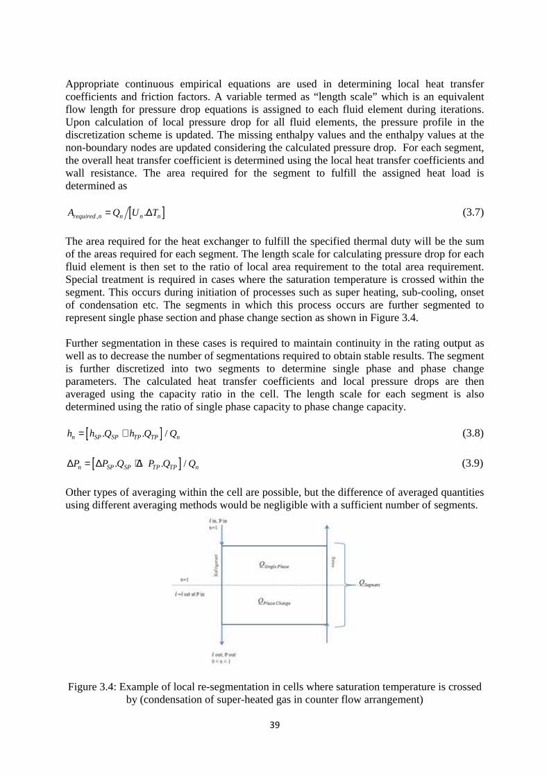
39

Appropriate continuous empirical equations are used in determining local heat transfer coefficients and friction factors. A variable termed as “length scale” which is an equivalent flow length for pressure drop equations is assigned to each fluid element during iterations. Upon calculation of local pressure drop for all fluid elements, the pressure profile in the discretization scheme is updated. The missing enthalpy values and the enthalpy values at the non-boundary nodes are updated considering the calculated pressure drop. For each segment, the overall heat transfer coefficient is determined using the local heat transfer coefficients and wall resistance. The area required for the segment to fulfill the assigned heat load is determined as

[ ], .required n n n nA Q U T= ∆ (3.7)

The area required for the heat exchanger to fulfill the specified thermal duty will be the sum of the areas required for each segment. The length scale for calculating pressure drop for each fluid element is then set to the ratio of local area requirement to the total area requirement. Special treatment is required in cases where the saturation temperature is crossed within the segment. This occurs during initiation of processes such as super heating, sub-cooling, onset of condensation etc. The segments in which this process occurs are further segmented to represent single phase section and phase change section as shown in Figure 3.4. Further segmentation in these cases is required to maintain continuity in the rating output as well as to decrease the number of segmentations required to obtain stable results. The segment is further discretized into two segments to determine single phase and phase change parameters. The calculated heat transfer coefficients and local pressure drops are then averaged using the capacity ratio in the cell. The length scale for each segment is also determined using the ratio of single phase capacity to phase change capacity.

[ ]. . /n SP SP TP TP nh h Q h Q Q= + (3.8)

[ ]. . /n SP SP TP TP nP P Q P Q Q∆ = ∆ + ∆ (3.9)

Other types of averaging within the cell are possible, but the difference of averaged quantities using different averaging methods would be negligible with a sufficient number of segments.

Figure 3.4: Example of local re-segmentation in cells where saturation temperature is crossed by (condensation of super-heated gas in counter flow arrangement)

40

Checks of the calculated pressure and enthalpy profiles are also done during this step. If conditions such as excessive pressure drop on the refrigerant side resulting in crossing temperature profiles are identified, the rating iterations are stopped and appropriate warnings are returned. Step 4: The final step in the iterative procedure involves determination of the wall temperature profile. In each segment, the wall node temperatures are determined using an energy balance.

,1 1 1 21

nWall E E E

E

UT T T T

h = − − (3.10)

,2 2 2 12

nWall E E E

E

UT T T T

h = − − (3.11)

The root mean square difference of the temperature from a previous iteration in all wall nodes is determined and is used as convergence criterion. The maximum error for wall temperature convergence is set to 1E-4, which will be usually achieved in less than ten iterations. The oversurface is finally determined as the ratio of the total area required to the total effective heat transfer area available. Because the current one-dimensional model cannot be used to determine the distribution of the fluids in the port manifolds, an empirical model is used to determine the flow maldistribution. This factor is then used as a factor on the calculated oversurface to account for the performance deterioration with large number of plates etc. Additional parameters such as the channel velocity, port velocity, port pressure drops, channel temperature profiles, wall temperature profiles, local heat transfer coefficients and pressure drops are returned as output in these rating calculations. 3.3.4 Number of segments required The number of segments required for stable rating predictions is determined for single phase and phase change applications. In single phase applications, the tests using two trans-critical Carbon Dioxide gas cooler cases with water on the secondary side are presented here. Two different operating pressures are used. For a higher operating pressure, the results became stable at around 100 segments and for lower operating pressure the results are stable for a very low number of segments. This is due to the internal temperature profiles and changed degree of variation of fluid properties at different pressures. Based on the results in selection, performance and rating calculations the number of segments for single phase calculations is set to 50. The variation of the predicted overall heat transfer coefficient with the number of segments in the stepwise rating method for transcritical CO2 and cascaded heat exchanger calculations are shown in Figure 3.5 and Figure 3.6, respectively.

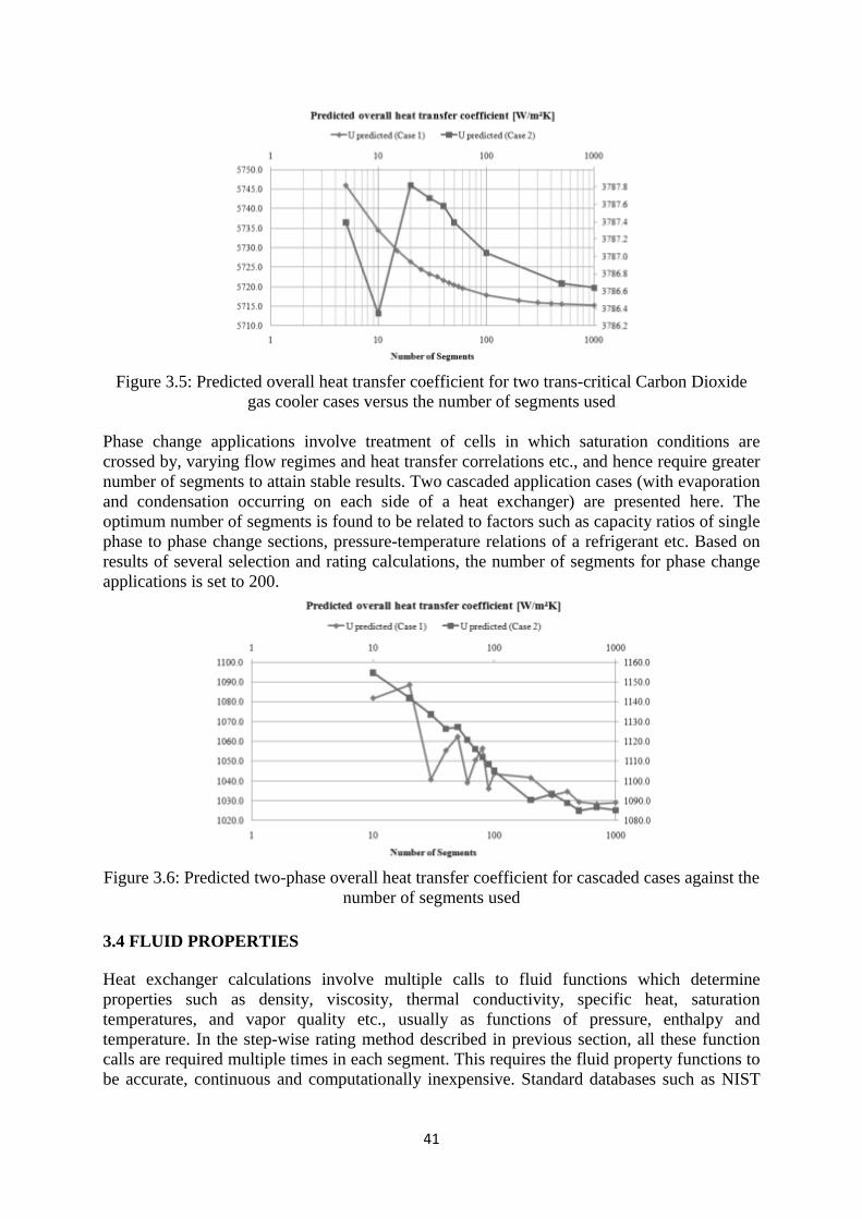
Figure 3.5: Predicted overall heat transfer coefficient for two trans

Phase change applications involve treatment of cells in which saturation conditions are crossed by, varying flow regimes and heat transfer correlations etc., and hence require number of segments to attain stable results. Two cascaded application cases (with and condensation occurring on each side of a heat exchanger) are presented here. The optimum number of segments is found to be related to factors such as capacity ratios of single phase to phase change sections, pressureresults of several selection and rating calculations, the number of segments for phase change applications is set to 200.

Figure 3.6: Predicted two

3.4 FLUID PROPERTIES Heat exchanger calculations involve multiple calls to fluid functions which determine properties such as density, viscosity, thermal conductivity, specific heat, saturation temperatures, and vapor quality etc., usutemperature. In the stepcalls are required multiple times in each segment. This requires the fluid property functions to be accurate, continuo

41

Figure 3.5: Predicted overall heat transfer coefficient for two transgas cooler cases versus the number of segments used

ge applications involve treatment of cells in which saturation conditions are crossed by, varying flow regimes and heat transfer correlations etc., and hence require number of segments to attain stable results. Two cascaded application cases (with and condensation occurring on each side of a heat exchanger) are presented here. The optimum number of segments is found to be related to factors such as capacity ratios of single phase to phase change sections, pressure-temperature relations oresults of several selection and rating calculations, the number of segments for phase change applications is set to 200.

Figure 3.6: Predicted two-phase overall heat transfer coefficient for cascaded cases against the number of segments used

3.4 FLUID PROPERTIES

Heat exchanger calculations involve multiple calls to fluid functions which determine properties such as density, viscosity, thermal conductivity, specific heat, saturation temperatures, and vapor quality etc., usually as functions of pressure, enthalpy and temperature. In the step-wise rating method described in previous section, all these function calls are required multiple times in each segment. This requires the fluid property functions to be accurate, continuous and computationally inexpensive. Standard databases such as NIST

41

Figure 3.5: Predicted overall heat transfer coefficient for two trans-critical Carbon Dioxide

gas cooler cases versus the number of segments used

ge applications involve treatment of cells in which saturation conditions are crossed by, varying flow regimes and heat transfer correlations etc., and hence require number of segments to attain stable results. Two cascaded application cases (with and condensation occurring on each side of a heat exchanger) are presented here. The optimum number of segments is found to be related to factors such as capacity ratios of single

temperature relations of a refrigerant etc. Based on results of several selection and rating calculations, the number of segments for phase change

phase overall heat transfer coefficient for cascaded cases against the r of segments used

Heat exchanger calculations involve multiple calls to fluid functions which determine properties such as density, viscosity, thermal conductivity, specific heat, saturation

ally as functions of pressure, enthalpy and wise rating method described in previous section, all these function

calls are required multiple times in each segment. This requires the fluid property functions to us and computationally inexpensive. Standard databases such as NIST

critical Carbon Dioxide

ge applications involve treatment of cells in which saturation conditions are crossed by, varying flow regimes and heat transfer correlations etc., and hence require greater number of segments to attain stable results. Two cascaded application cases (with evaporation and condensation occurring on each side of a heat exchanger) are presented here. The optimum number of segments is found to be related to factors such as capacity ratios of single

f a refrigerant etc. Based on results of several selection and rating calculations, the number of segments for phase change

phase overall heat transfer coefficient for cascaded cases against the

Heat exchanger calculations involve multiple calls to fluid functions which determine properties such as density, viscosity, thermal conductivity, specific heat, saturation

ally as functions of pressure, enthalpy and wise rating method described in previous section, all these function

calls are required multiple times in each segment. This requires the fluid property functions to us and computationally inexpensive. Standard databases such as NIST

42

REFPROP provide accurate and continuous fluid properties but slow down the calculation procedure when referred through alternate programming platforms and frameworks. It is often customary to use one-dimensional curve fits for liquid and saturated state properties (temperature as the independent variable) and two-dimensional models for vapor and super-critical properties (pressure and temperature/ enthalpy as independent variables). The accuracy of these models is limited in cases where fluid properties change significantly. Using piecewise models introduces continuity problems at the model boundaries and hence are not desired. The current section describes two local interpolation models which can be used for accurate and efficient retrieval of fluid properties. 3.4.1 Linear interpolation of bi-dimensional meshes The method of obtaining refrigerant properties using linear interpolation of two-dimensional property maps is presented by Corberán et al. Property maps were created by collecting data from NIST REFPROP for various refrigerants. The sub-cooled, super-heated and super-critical properties are obtained as functions of pressure/temperature and density/temperature. The saturation property maps are obtained as function of saturation pressure. Finite difference approximation is used for missing properties close to the critical temperature. These maps represent the nodal information of the parallelograms that are formed between the constant pressure, constant temperature and constant density lines. When a property needs to be evaluated, all of the boundary nodes of the parallelogram containing the independent variable are searched. The parallelogram is then treated as an isoparametric finite element for linear local interpolation. Using this method, the properties in the entire pressure-enthalpy domain are determined with an error less than 1%. The time required to obtain 1000 properties is calculated and the developed method showed 100 times improvement as compared to the equation of state based iterative methods used in NIST REFPROP. 3.4.2 Finite Grid Interpolation Method for Accurate Fluid Properties An improved local interpolation based method for obtaining accurate and continuous fluid properties is developed for the current study. The method is developed based on the following goals:

- Elimination of the need of developing maps with different independent variables - Elimination of need for domain mapping required for isoparametric elements, hence

only linear, quad and triangular finite elements should be used - Possibility of indexing and using of efficient data structures and data types for

improvement of search speed and decreasing memory requirements - Ability to enhance local mesh in the regions where fluid properties vary significantly - Possibility to use Lagrangian interpolation where properties are missing in standard

databases such as NIST REFPROP. - Ability to obtain properties from a variety of data sources - Possibility to compress the developed property maps for reducing the size of the

installation files. - Possibility to use smart search algorithms and information from previous calculations

to decrease the overall time taken by a rating calculation - Efficient binary methods for obtaining results for inverse functions (finding an

independent variable when a dependent variable is available)

43

The steps in creating a property map for a given refrigerant is described below. Step 1: The boundaries of the pressure-enthalpy domain where the properties should be obtained are initially identified. The property maps are generated separately for sub-critical and super-critical regions while preserving continuity at the domain interface. The saturation region is initially divided into a number of pressure steps. These pressure steps are placed in a vector for indexing purpose. This would also create a list of bub-line (liquid line) and dew-line saturation enthalpies. Due to the shape of the dew curve, it is possible to obtain duplicate values for the dew enthalpies. These duplicate enthalpies are eliminated for smooth operation of the search function. The sub-cooled liquid region and the superheated region are discretized further at various enthalpies. The resulting bulk and saturation enthalpies are sorted and placed in a vector for indexing. The used pressures and enthalpies in the subcritical and supercritical regions would form a finite element mesh with two-node line elements representing the saturation line, three-node triangle elements close to the bub and dew regions and four-node quad elements in the supercritical and bulk subcritical regions as shown in Figure 3.7. The saved pressure and enthalpy values are further indexed to identify the region to which they belong. (Supercritical, vapor, liquid, saturation region etc)

Figure 3.7: Schematic of the developed two-dimensional property map in the pressure-enthalpy domain for a refrigerant

Step 2: At the various nodes obtained from the saved pressure enthalpy combinations, properties such as density, viscosity, thermal conductivity, specific heat, entropy etc., are obtained and saved in a separate data structure. The node property collections are linked to the pressure and enthalpy vectors by index variables to simplify the search procedure. In case of missing values from the standard data source, Lagrangian interpolation of the nearby nodes is used to obtain the properties. This procedure is described by Gullapalli (2011a). Step 3: The linear interpolation scheme is then used to verify the accuracy of the calculated properties at thousands of random points in order to determine if the developed maps are sufficient. In the regions where the accuracy is low additional pressure and enthalpy levels are added. The refinement of the mesh continues until the maximum deviation in all the properties is lower than 1%. The collected data is then custom-serialized and custom

44

compressed to decrease the storage memory requirement. The average size of compressed property maps for each refrigerant is around 200 kB. When a property needs to be determined for a given pressure and enthalpy, the first step would be to determine the element containing the specified pressure and enthalpy. The binary search on the pressure and enthalpy indexes identifies the state and the surrounding nodes which forms the finite element in a very efficient way. Depending on the state and the element type, appropriate shape functions are used for local linear interpolation. The shape functions for these elements and their characteristics can be found in Jaluria et al. (2003). Using these shape functions all the properties that are saved in the nodes can be determined in one query. The developed method serves excellently the pressure-enthalpy based step-wise rating method with its quick and continuous fluid property functions. When compared to the time required for a Microsoft .net application which directly refers to NIST REFPROP for fluid properties, the developed method demonstrated excellent improvement in calculation speed (Gullapalli, 2011a). 3.5 EVALUATION OF CONSTANTS IN EMPIRICAL CORRELATIONS The constants and enhancement/deterioration factors in the empirical correlations for heat transfer and pressure drop used in the rating methods needs to the evaluated. Various linear and nonlinear regression based techniques are listed in the literature for the standard form of the equations. Some of these methods require specific laboratory testing methodology. For commercial applications, optimization based parameter estimation provides an alternative to regression based techniques. Software applications based on search methods are developed for calibration of correlations used in this study. These evaluation methods are briefly described below. 3.5.1 Single Phase Evaluation Single phase evaluation involves determination of empirical constants in thermal and hydraulic correlations using laboratory test data. The test data obtained usually contains the inlet and outlet temperatures, mass flow rates and pressure drops on the hot and cold sides. In the initial stage, the test data is filtered to remove the test points with bad energy balance and those with parameters which fall out of the range of the measurement equipment used in the test rig. The test points with minimum temperature difference less than 3K are also disregarded because they are associated with higher uncertainty. The average heat load and the measured overall heat transfer coefficient are obtained as

( )0.5 p ph cQ mC T mC T = ∆ + ∆ ɺ ɺ (3.12)

( )lab LMTDU Q A T= ∆ (3.13)

The bulk overall heat transfer coefficient in the rating calculation for each test point is calculated as

11 1model h c rU h h W

−− − = Ω + + (3.14)

45

Ω is a correction factor that is used to compensate the deterioration in heat transfer at the end plates and for multiple passes. The resistance at the wall ( rW ) includes contributions from the thermal resistance, fouling and air resistance in double plate models. The measured and modeled overall convective resistances are obtained as

1 1model h cZ h h− −= + (3.15)

( )lab lab rZ U W= Ω − (3.16)

The heat transfer coefficient on each side is calculated as

h

Nuh

D

λ= Ψ (3.17)

The correction factor (Ψ ) is used to compensate for the viscosity variation at the bulk and wall conditions. In this evaluation, the heat transfer performances for the hot and cold sides are represented by the power curve relation presented by Bogaert (1994)

Re Prn yNu c= Ψ (3.18) Rearranging the terms in Equation (3.15), the modeled overall convective resistance becomes

modelRe Re Pr

hn n y

h c

DZ where

c c

ξ ξ ξλ

= + = Ψ Ψ (3.19)

The constant c usually varies from 0.1 to 0.7 and n varies from 0.5 to 0.8 for brazed plate heat exchangers. These empirical constants depend strongly on the plate geometry. Equation (3.19) is a non-linear equation because the viscosity variation factor depends on the wall conditions which in turn depend on the convective resistance on both the sides. The root mean square difference between the modeled and measured overall convective resistance is calculated as

( )0.5

2model

1

1 N

Z labZ ZN

δ

= − ∑ (3.20)

The evaluation of the measured single phase test data now reduces to a constrained optimization problem with the empirical constants as the parameters and the RMS error (Zδ ) as the objective function. Various techniques can be used to determine the empirical constants which result in the least RMS error. Briggs and Young (1969) presented a non-linear least square technique which is based on the Wilson plot method. In the current study, gradient based optimization techniques such as the Gauss-Newton method and meta-heuristic methods such as direct search methods are used to solve the optimization problem. For symmetric heat exchanger models the number of empirical constants reduces to two because the performance characteristics on the warm and cold sides are assumed to be similar. The pressure drop correlations evaluation is similar to the heat transfer correlation evaluation because the single phase friction factor can be modeled as power function of Reynolds number. For fully turbulent regions (typically Re > 500), the direct search method is proved to be successful in

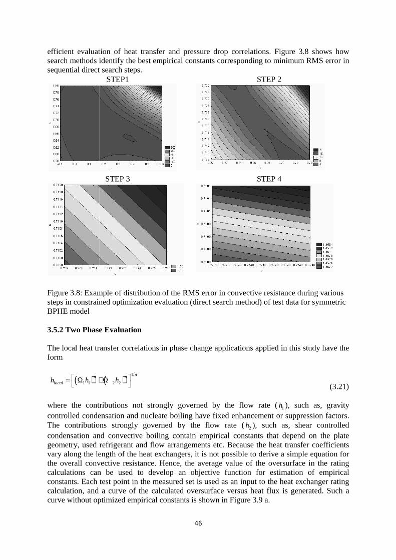
efficient evaluation of heat transfer and pressure drop correlations. search methods identifysequential direct search steps.

Figure 3.8: Example of distribution of the RMS error in convective resistance during various steps in constrained optimization evaluation (direct search method) of test data for symmetric BPHE model 3.5.2 Two Phase The local heat transfer correlations in phase change applications form

( )1 1 2 2n n

localh h h = Ω + Ω

where the contributions not strongly governed bycontrolled condensation and nucleate boiling have fixed enhThe contributions strongly governed by the flow rate (condensation and convective boiling contain empirical constants that depend on the plate geometry, used refrigerant and flow arrangements etc. Because the heat transfer coefficients vary along the length of the heat exchangers,the overall convective resistance. Hence, the average value ofcalculations can be used to develop an objective function for estimation of empirical constants. Each test poincalculation, and a curve of curve without optimized empirical constants is shown in

46

efficient evaluation of heat transfer and pressure drop correlations. search methods identify the best empirical constants corresponding to minimum RMS error in sequential direct search steps.

STEP1

STEP 3

Figure 3.8: Example of distribution of the RMS error in convective resistance during various steps in constrained optimization evaluation (direct search method) of test data for symmetric

3.5.2 Two Phase Evaluation

The local heat transfer correlations in phase change applications

( )1

1 1 2 2

nn nh h h = Ω + Ω

where the contributions not strongly governed bycontrolled condensation and nucleate boiling have fixed enh

he contributions strongly governed by the flow rate (condensation and convective boiling contain empirical constants that depend on the plate geometry, used refrigerant and flow arrangements etc. Because the heat transfer coefficients vary along the length of the heat exchangers, it is not possible to derive a simple equation for

overall convective resistance. Hence, the average value ofcalculations can be used to develop an objective function for estimation of empirical constants. Each test point in the measured set is used as an input to the heat exchanger rating calculation, and a curve of the calculated oversurface versus heat flux is generated. Such a curve without optimized empirical constants is shown in

46

efficient evaluation of heat transfer and pressure drop correlations. Figure best empirical constants corresponding to minimum RMS error in

STEP 2

STEP 4

Figure 3.8: Example of distribution of the RMS error in convective resistance during various steps in constrained optimization evaluation (direct search method) of test data for symmetric

The local heat transfer correlations in phase change applications applied in this study

where the contributions not strongly governed by the flow rate (1h ), such as, gravity controlled condensation and nucleate boiling have fixed enhancement or suppression factors.

he contributions strongly governed by the flow rate ( 2h ), such as, shear controlled condensation and convective boiling contain empirical constants that depend on the plate geometry, used refrigerant and flow arrangements etc. Because the heat transfer coefficients

it is not possible to derive a simple equation for overall convective resistance. Hence, the average value of the oversurface in the rating

calculations can be used to develop an objective function for estimation of empirical t in the measured set is used as an input to the heat exchanger rating

calculated oversurface versus heat flux is generated. Such a curve without optimized empirical constants is shown in Figure 3.9 a.

3.8 shows how best empirical constants corresponding to minimum RMS error in

Figure 3.8: Example of distribution of the RMS error in convective resistance during various steps in constrained optimization evaluation (direct search method) of test data for symmetric

in this study have the

(3.21)

), such as, gravity ancement or suppression factors.

), such as, shear controlled condensation and convective boiling contain empirical constants that depend on the plate geometry, used refrigerant and flow arrangements etc. Because the heat transfer coefficients

it is not possible to derive a simple equation for oversurface in the rating

calculations can be used to develop an objective function for estimation of empirical t in the measured set is used as an input to the heat exchanger rating

calculated oversurface versus heat flux is generated. Such a

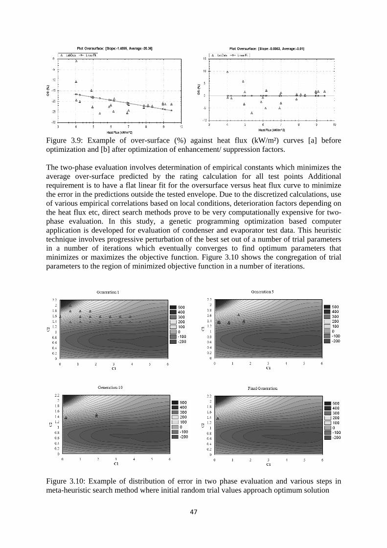
47

Figure 3.9: Example of over-surface (%) against heat flux (kW/m²) curves [a] before optimization and [b] after optimization of enhancement/ suppression factors. The two-phase evaluation involves determination of empirical constants which minimizes the average over-surface predicted by the rating calculation for all test points Additional requirement is to have a flat linear fit for the oversurface versus heat flux curve to minimize the error in the predictions outside the tested envelope. Due to the discretized calculations, use of various empirical correlations based on local conditions, deterioration factors depending on the heat flux etc, direct search methods prove to be very computationally expensive for two-phase evaluation. In this study, a genetic programming optimization based computer application is developed for evaluation of condenser and evaporator test data. This heuristic technique involves progressive perturbation of the best set out of a number of trial parameters in a number of iterations which eventually converges to find optimum parameters that minimizes or maximizes the objective function. Figure 3.10 shows the congregation of trial parameters to the region of minimized objective function in a number of iterations.

Figure 3.10: Example of distribution of error in two phase evaluation and various steps in meta-heuristic search method where initial random trial values approach optimum solution

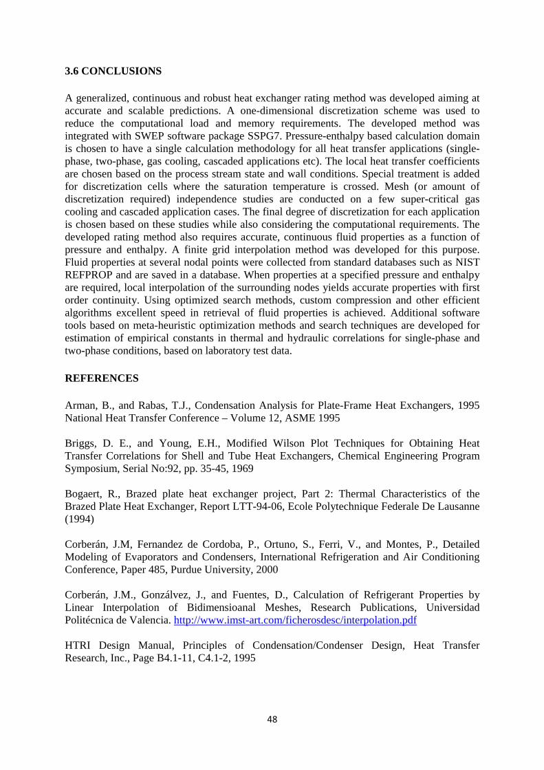
48

3.6 CONCLUSIONS A generalized, continuous and robust heat exchanger rating method was developed aiming at accurate and scalable predictions. A one-dimensional discretization scheme was used to reduce the computational load and memory requirements. The developed method was integrated with SWEP software package SSPG7. Pressure-enthalpy based calculation domain is chosen to have a single calculation methodology for all heat transfer applications (single-phase, two-phase, gas cooling, cascaded applications etc). The local heat transfer coefficients are chosen based on the process stream state and wall conditions. Special treatment is added for discretization cells where the saturation temperature is crossed. Mesh (or amount of discretization required) independence studies are conducted on a few super-critical gas cooling and cascaded application cases. The final degree of discretization for each application is chosen based on these studies while also considering the computational requirements. The developed rating method also requires accurate, continuous fluid properties as a function of pressure and enthalpy. A finite grid interpolation method was developed for this purpose. Fluid properties at several nodal points were collected from standard databases such as NIST REFPROP and are saved in a database. When properties at a specified pressure and enthalpy are required, local interpolation of the surrounding nodes yields accurate properties with first order continuity. Using optimized search methods, custom compression and other efficient algorithms excellent speed in retrieval of fluid properties is achieved. Additional software tools based on meta-heuristic optimization methods and search techniques are developed for estimation of empirical constants in thermal and hydraulic correlations for single-phase and two-phase conditions, based on laboratory test data. REFERENCES Arman, B., and Rabas, T.J., Condensation Analysis for Plate-Frame Heat Exchangers, 1995 National Heat Transfer Conference – Volume 12, ASME 1995 Briggs, D. E., and Young, E.H., Modified Wilson Plot Techniques for Obtaining Heat Transfer Correlations for Shell and Tube Heat Exchangers, Chemical Engineering Program Symposium, Serial No:92, pp. 35-45, 1969 Bogaert, R., Brazed plate heat exchanger project, Part 2: Thermal Characteristics of the Brazed Plate Heat Exchanger, Report LTT-94-06, Ecole Polytechnique Federale De Lausanne (1994) Corberán, J.M, Fernandez de Cordoba, P., Ortuno, S., Ferri, V., and Montes, P., Detailed Modeling of Evaporators and Condensers, International Refrigeration and Air Conditioning Conference, Paper 485, Purdue University, 2000 Corberán, J.M., Gonzálvez, J., and Fuentes, D., Calculation of Refrigerant Properties by Linear Interpolation of Bidimensioanal Meshes, Research Publications, Universidad Politécnica de Valencia. http://www.imst-art.com/ficherosdesc/interpolation.pdf HTRI Design Manual, Principles of Condensation/Condenser Design, Heat Transfer Research, Inc., Page B4.1-11, C4.1-2, 1995

49

Gullapalli, V.S., Condensation in Compact Brazed Plate Heat Exchangers: Evaluation and Performance Analysis, Heat SET 2007, Heat Transfer in Components and Systems for Sustainable Energy Technologies, Chambery, France, 2007 Gullapalli, V.S., On Performance Analysis of Plate Heat Exchangers, Thesis for the Degree of Licentiate in Engineering, ISRN LUTMDN/TMHP-08/7055-SE, 2008 Gullapalli, V.S., and Sundén, B., Generalized Performance Analysis of Compact Brazed Plate Heat Exchangers, Proceedings of the 21st National & 10th ISHMT-ASME Heat and Mass Transfer Conference, IIT Madras, India, December 27-30, 2011a Gullapalli, V.S., and Sundén, B., Condensation and Evaporation in Compact Brazed Plate Heat Exchangers: Generalized Rating Method, Proceedings of the 21st National & 10th ISHMT-ASME Heat and Mass Transfer Conference, IIT Madras, India, December 27-30, 2011b Jaluria, Y., and Torrance, K.E., Computational Heat Transfer, Taylor & Francis, London, 2003 Mancin. S., Del Col, D., and Rossetto. L., Superheated Vapor Condensation of R410A: A Design Procedure, IRC 2011, Prague, 2011 Mayta Tito, J.M., Ortega Sotomayor, P., and Parise, J.A.R., Study of Alternate Refrigerants for a Cascade Vapor Compression Cycle Employing Brazed Plate Heat Exchangers, IRC 2011, Prague, 2011 Pacio, J., and Dorao, C., Design Considerations for the Sizing of High Effectiveness Two-Phase Flow Heat Exchangers, IRC 2011, Prague, 2011 Strelow, O., A General Calculation Method for Plate Heat Exchangers, International Journal of Thermal Sciences (39), pp. 645-658, 2000 Wang, L., Christensen, R., and Sundén, B., Calculation Procedure for Steam Condensation in Plate Heat Exchangers, Compact Heat Exchangers and Enhancement Technology for the Process Industry, Begell House, pp. 479-484, 1999

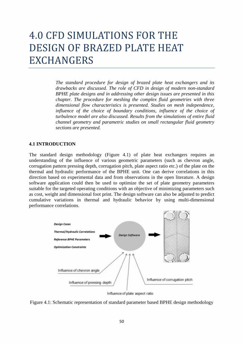
4.0 CFD SIMULATIONS FOR

DESIGN OF

EXCHANGERS

The standard procedure for design of brazed plate heat exchangers and its drawbacks are discussed. The role of CFD in design of modern nonBPHE plate designs and in addressing other dchapter. The procedure for meshing the complex fluid geometries with three dimensional flow characteristics is presented. Studies on mesh independencinfluence of the choice of boundary conditions, influence of the turbulence model are also discussed. Results from the simulations of entire fluid channel geometry and parametric studies on small rectangular fluid geometry sections are presented.

4.1 INTRODUCTION The standard design methodologyunderstanding of the influence of various geometric parameters (such as chevron angle, corrugation pattern pressing depth, corrugation pitch, plate aspect ratio etc.) of the plate on the thermal and hydraudirection based on experimental data and from observations in the open literature. A design software application could then be used to optimize the set of plate geometry parameters suitable for the targeted operating conditions with an objective of minimizing parameters such as cost, weight and dimensional foot print. The design software can also be adjusted to predict cumulative variations in thermal and hydraulic behavior by using multiperformance correlations.

Figure 4.1: Schematic representation of standard parameter based BPHE design methodology

50

CFD SIMULATIONS FOR

DESIGN OF BRAZED PLATE HEAT

EXCHANGERS

The standard procedure for design of brazed plate heat exchangers and its drawbacks are discussed. The role of CFD in design of modern nonBPHE plate designs and in addressing other dchapter. The procedure for meshing the complex fluid geometries with three dimensional flow characteristics is presented. Studies on mesh independencinfluence of the choice of boundary conditions, influence of the turbulence model are also discussed. Results from the simulations of entire fluid channel geometry and parametric studies on small rectangular fluid geometry sections are presented.

4.1 INTRODUCTION

The standard design methodology (Figure 4.1)understanding of the influence of various geometric parameters (such as chevron angle, corrugation pattern pressing depth, corrugation pitch, plate aspect ratio etc.) of the plate on the thermal and hydraulic performance of the BPHE unit. One can derive direction based on experimental data and from observations in the open literature. A design software application could then be used to optimize the set of plate geometry parameters

ble for the targeted operating conditions with an objective of minimizing parameters such as cost, weight and dimensional foot print. The design software can also be adjusted to predict cumulative variations in thermal and hydraulic behavior by using multiperformance correlations.

Figure 4.1: Schematic representation of standard parameter based BPHE design methodology

50

CFD SIMULATIONS FOR THE

BRAZED PLATE HEAT

The standard procedure for design of brazed plate heat exchangers and its drawbacks are discussed. The role of CFD in design of modern nonBPHE plate designs and in addressing other design issues are presented in this chapter. The procedure for meshing the complex fluid geometries with three dimensional flow characteristics is presented. Studies on mesh independencinfluence of the choice of boundary conditions, influence of the turbulence model are also discussed. Results from the simulations of entire fluid channel geometry and parametric studies on small rectangular fluid geometry

(Figure 4.1) of plate heat exchangers requires an understanding of the influence of various geometric parameters (such as chevron angle, corrugation pattern pressing depth, corrugation pitch, plate aspect ratio etc.) of the plate on the

lic performance of the BPHE unit. One can derive correlationsdirection based on experimental data and from observations in the open literature. A design software application could then be used to optimize the set of plate geometry parameters

ble for the targeted operating conditions with an objective of minimizing parameters such as cost, weight and dimensional foot print. The design software can also be adjusted to predict cumulative variations in thermal and hydraulic behavior by using multi

Figure 4.1: Schematic representation of standard parameter based BPHE design methodology

BRAZED PLATE HEAT

The standard procedure for design of brazed plate heat exchangers and its drawbacks are discussed. The role of CFD in design of modern non-standard

esign issues are presented in this chapter. The procedure for meshing the complex fluid geometries with three dimensional flow characteristics is presented. Studies on mesh independence, influence of the choice of boundary conditions, influence of the choice of turbulence model are also discussed. Results from the simulations of entire fluid channel geometry and parametric studies on small rectangular fluid geometry

of plate heat exchangers requires an understanding of the influence of various geometric parameters (such as chevron angle, corrugation pattern pressing depth, corrugation pitch, plate aspect ratio etc.) of the plate on the

correlations in this direction based on experimental data and from observations in the open literature. A design software application could then be used to optimize the set of plate geometry parameters

ble for the targeted operating conditions with an objective of minimizing parameters such as cost, weight and dimensional foot print. The design software can also be adjusted to predict cumulative variations in thermal and hydraulic behavior by using multi-dimensional

Figure 4.1: Schematic representation of standard parameter based BPHE design methodology

51

The continuous demand for improved efficiency in industrial, heating and refrigeration application requires investigations on non-standard plate patterns that evolve for suiting the local flow physics, refrigerant properties and the available temperature approach. The aforementioned design tools will be of less use in those situations due to the non-availability of performance-geometry linking correlations. The development of these relations for a large set of geometric parameters at various flow conditions from experimental methods is not a viable option. In recent years, the operating envelope of plate heat exchanges has been widened significantly resulting in design of units with relatively large dimensions. This scaling of heat exchangers would introduce additional problems such as non-uniform distribution of fluids within the channel etc. The performance-geometry correlations developed from experimental data of relatively small units cannot be used effectively for larger BPHE designs. Additionally, a large variation in performance can be obtained by local geometric modifications, such as opening of the closed regions due to large braze junctions. The changes that these modifications bring cannot be quantified in a simple way to include them as correlations in standard design software. These limitations call for a use of simulation tools such as computational fluid dynamics for determining the thermal and hydraulic performance during the design of modern plate heat exchangers. 4.2 COMPUTATIONAL FLUID DYNAMICS The application of computational fluid dynamics (CFD) tools involve solving of a set of multi-dimensional differential transport equations developed for flow transport characteristics such as mass flow, momentum, internal energy and other turbulence characteristics over a fluid domain of interest. This set of differential equations is augmented with equations for fluid thermo-physical properties and auxiliary conditions such as initial and boundary conditions. The three-dimensional fluid domain of interest is discretized into a number of cells characterized by nodes, edges and faces. The integral forms of the transport equations are then converted into approximate algebraic equations for each of these cells and the resulting set of nonlinear algebraic system of equations for the entire fluid domain is solved using various semi-explicit schemes. 4.2.1. Governing Equations The conservative (or divergence) form of the transport equation for a general variable φ (conserved property per unit mass) can be formulated as

( ) ( ) ( )div u div St

ρφρφ φ

∂+ = Γ ∇ +

∂

(4.1)

where Γ represents the diffusion coefficient and S represents the additional source terms. The integral form of the equation for a finite volume can be formulated using Gauss divergence theorem as

( ) ( ). .V A A V

dV n u dA n dA SdVt

ρφ ρφ φ ∂ + = Γ∇ + ∂ ∫ ∫ ∫ ∫

(4.2)

where n

in the normal vector to the surface element dA. The principle conserved properties per unit mass in case of fluid flow are unity (mass conservation), directional velocity components (momentum conservation) and specific energy (energy conservation).

52

The Lagrangian (or the non-conservative) approach involves rate of changes of the aforementioned properties following a fluid particle. The rate of change of the conserved quantity per unit mass per unit volume in this approach is represented by using a substantial derivative

.D

uDt t

φ φρ ρ φ∂ = + ∇ ∂

(4.3)

The Eulerian (or conservative) approach involves the rate of change of a conserved quantity with respect to a fixed finite volume in the fluid domain. The rate of change of a conserved quantity per unit mass per unit volume is then represented as

( ) ( )div ut

ρφρφ

∂+

∂

(4.4)

The conservative form of the unsteady compressible mass conservation equation is given by

( ) 0div ut

ρ ρ∂ + =∂

(4.5)

The momentum conservation equation primarily involves the momentum changes induced by the pressure forces and viscous forces. The additional body forces are usually appended into the conservation equation as momentum source terms. The unsteady compressible momentum equation for the finite fluid volume is given in tensor notation as

( ) ( ) ( ) M

udiv u u P div S

t

ρρ τ

∂+ ⊗ = −∇ + +

∂

(4.6)

where ⊗ represents the tensor product of two vectors and MS is the momentum source term.

The above equation is used for formulation of Navier-Stokes equations which uses relations between shear stresses and velocity gradients that are applied to Newtonian fluids. In these equations, the secondary viscosity that relates stresses to volumetric deformation is represented as a function of dynamic viscosity (Schlichting, 1979). Hence, in Navier-Stokes equation, the stress tensor is related to the strain rate as

( ) 2( )

3T

ku u div uτ µ δ = ∇ + ∇ −

(4.7)

where kδ represents the Kronecker delta function and T is the vector transpose operator.

The total energy equation for unsteady compressible flow involves conservation of the total enthalpy. The energy flux due to heat conduction is represented using Fourier’s law of conduction. Additional energy terms include work due to viscous stresses, work due to external momentum sources and other energy sources. The total energy equation can hence be represented as

( ) ( ) ( ) ( ). .tt M E

i Pdiv ui div T div u u S S

t t

ρρ λ τ

∂ ∂− + = ∇ + + +∂ ∂

(4.8)

53

The total enthalpy in the above equation is defined as

2 21 1

2 2t

Pi i u e u

ρ= + = + +

(4.9)

The system of equations representing the fluid flow contains four unknown thermodynamic quantities: density, pressure, internal energy and temperature. The relationship between these variables can be obtained by the assumption of thermodynamic equilibrium. It is generally sufficient to state two state variables in this condition and equations of state can be used to calculate the other thermodynamic state variables. 4.2.2. Turbulence Modeling The Reynolds averaged Navier-Stokes (RANS) modeling for turbulence used in this study involves generating a modified set of transport equations by introducing averaged and fluctuating velocity components. The velocity vector can be divided into a time averaged and time varying component as

u U u′= +

(4.10) The set of transport equations for fluid flow using the above definition takes the form

( ) 0div Ut

ρ ρ∂ + =∂

(4.11)

( ) ( ) ( ) M

Udiv U U div u u S

t

ρρ τ ρ

∂+ ⊗ = − ⊗ +

∂

(4.12)

( ) ( ) ( )tt E

i Pdiv Ui div T ui div U S

t t

ρ ρ λ ρ τ∂ ∂− + = ∇ − + +∂ ∂

(4.13)

The mean total enthalpy in the above equations would also contain the contributions from turbulent kinetic energy

2 21 1where

2 2ti i U k k u= + + =

(4.14)

The above set of equations introduces a closure problem with six undefined Reynolds stresses u uρ ⊗

(three normal and three shear stresses). The eddy viscosity turbulence models attempt

to relate the Reynolds stresses to mean velocity gradients and a turbulent viscosity (tµ )

similar to the Navier-Stokes equation for laminar flow.

( ) 2( )

3

T

t k tu u U U k div Uρ µ δ ρ µ ⊗ = ∇ + ∇ − − +

(4.15)

The detailed derivation of turbulent transport equations and Reynolds stresses can be found in Sjögren (1997) and ANSYS (2006). The RANS models used in this study are briefly presented here.

54

The k ε− turbulence model relates the turbulence viscosity to the turbulent kinetic energy and the viscous dissipation of turbulent kinetic energy (ε ) using dimensional analysis as

2

t

kCµµ ρ

ε= (4.16)

The values for local turbulent kinetic energy and dissipation rate are obtained from their respective transport equations which are of the form

( ) ( ) ( ) ( )tdiv U div P Dt

ρφ ρφ µ φ φ φ∂ + = ∇ + +∂

(4.17)

The turbulence production term ( )P φ is a function of turbulent viscosity and mean

deformation tensor whereas the dissipation term ( )D φ is function of the turbulence intensity

and dissipation rate. The system of equations (4.17) contains five constants which are determined by data fitting to observations from a wide range of turbulent flows. The k ω− turbulence model expresses the turbulent viscosity as a function of turbulent kinetic energy and the turbulent frequency.

t

kµ ρω

= (4.18)

The Wilcox k ω− model formulates a system of transport equations of the form (4.17) for turbulent kinetic energy and turbulent frequency and involves five empirical constants. The k ω− model has an advantage over k ε− formulations in preventing the use of complex nonlinear damping functions for low Reynolds flows. The required near wall grid resolution is also less severe for the k ω− model. However, the Wilcox formulations show strong sensitivity to freestream conditions and the solutions are strongly depending on the turbulent frequency specified at the inlet. The baseline k ω− model solves the problem by using blending of the k ω− model near the wall and k ε− model in free stream conditions. These models are known to overpredict the turbulent viscosity because they do not account for transport of turbulent shear stress. The Shear Stress Transport (SST) turbulence model extends the baseline k ω− model by addition of limiters to the formulation of the turbulent viscosity. (ANSYS 2006). The Reynolds stress turbulence model formulations involve transport equations of all components of the Reynolds stress tensor and turbulent kinetic energy dissipation rate. The transport equation for the Reynolds stresses takes the form

( ) ( )22 2

3 3 k

R kdiv UR P R div c R

t

ρ ρ µ ρ δ ρεε

∂ + = + Π + + − ∂

(4.19)

where R u u= ⊗

The production term ( )P R and pressure-strain correlations Π are given by additional

equations. A transport equation for ε is also included because it appears in transport equation of the Reynolds stresses. Various RSM models with different empirical constants in equation set (4.19) are available in ANSYS (2006).

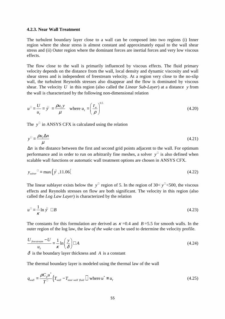
55

4.2.3. Near Wall Treatment The turbulent boundary layer close to a wall can be composed into two regions (i) Inner region where the shear stress is almost constant and approximately equal to the wall shear stress and (ii) Outer region where the dominant forces are inertial forces and very low viscous effects. The flow close to the wall is primarily influenced by viscous effects. The fluid primary velocity depends on the distance from the wall, local density and dynamic viscosity and wall shear stress and is independent of freestream velocity. At a region very close to the no-slip wall, the turbulent Reynolds stresses also disappear and the flow is dominated by viscous shear. The velocity U in this region (also called the Linear Sub-Layer) at a distance y from the wall is characterized by the following non-dimensional relation

0.5

where wu yUu y u

uτ

ττ

ρ τµ ρ

+ + = = = =

(4.20)

The y+ in ANSYS CFX is calculated using the relation

u ny τρ

µ+ ∆= (4.21)

n∆ is the distance between the first and second grid points adjacent to the wall. For optimum performance and in order to run on arbitrarily fine meshes, a solver y+ is also defined when scalable wall functions or automatic wall treatment options are chosen in ANSYS CFX.

( )max ,11.06solvery y+ += (4.22)

The linear sublayer exists below the y+ region of 5. In the region of 30<y+ <500, the viscous effects and Reynolds stresses on flow are both significant. The velocity in this region (also called the Log Law Layer) is characterized by the relation

1lnu y B

κ+ += + (4.23)

The constants for this formulation are derived as κ =0.4 and B =5.5 for smooth walls. In the outer region of the log law, the law of the wake can be used to determine the velocity profile.

1lnfreestreamU U y

Auτ κ δ

− = +

(4.24)

δ is the boundary layer thickness and A is a constant The thermal boundary layer is modeled using the thermal law of the wall

( )*

*wherepwall wall near wall fluid

C uq T T u u

T τ

ρ+= − ≡ (4.25)

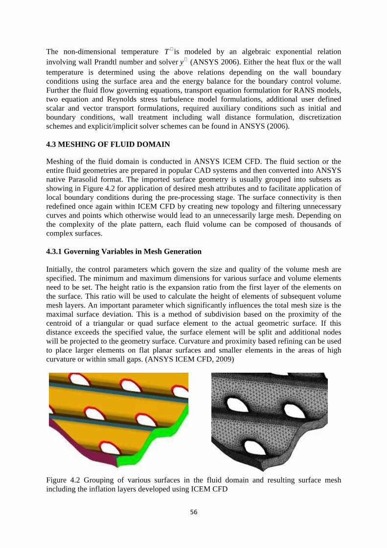
The non-dimensional temperature involving wall Prandtl number and solvertemperature is determined using the above relations depending on the wall boundary conditions using the surface area and the energy balance for the boundary control volume. Further the fluid flow governing equations, transptwo equation and Reynolds stress turbulence model formulations, additional user defined scalar and vector transport formulations, required auxiliary conditions such as initial and boundary conditions, wall treatmenschemes and explicit/implicit solver schemes can be found in ANSYS (2006). 4.3 MESHING OF FLUID DOMAIN Meshing of the fluid domain is conducted in ANSYS ICEM CFD. The fluid section or the entire fluid geometries are prepared native Parasolid format. The imported surface geometry is usually grouped into sushowing in Figure 4.2local boundary conditions during the preredefined once again within ICEM CFD by creating new topocurves and points which otherwise would lead to an unnecessarily large mesh. Depending on the complexity of the plate pattern, each fluid volume can be composed of thousands of complex surfaces. 4.3.1 Governing Variables in Initially, the control parameters which govern the size and quality of the volume mesh are specified. The minimum and maximum dimensions for various surface and volume elements need to be set. The height ratio is the expansion ratio from tthe surface. This ratio will be used to calculate the height of elements of subsequent volume mesh layers. An important parameter which significantly influences the total mesh size is the maximal surface deviation. This iscentroid of a triangular or quad surface element to the actual geometric surface. If this distance exceeds the specified value, the surface element will be split and additional nodes will be projected to place larger elements on flat planar surfaces and smaller elements in the areas of high curvature or within small gaps. (ANSYS ICEM CFD, 2009)

Figure 4.2 Grouping of varioincluding the inflation layers developed using ICEM CFD

56

dimensional temperature T+ is modeled by an algebraic exponential relation involving wall Prandtl number and solvery+ (ANSYS 2006). temperature is determined using the above relations depending on the wall boundary conditions using the surface area and the energy balance for the boundary control volume.

fluid flow governing equations, transptwo equation and Reynolds stress turbulence model formulations, additional user defined scalar and vector transport formulations, required auxiliary conditions such as initial and boundary conditions, wall treatment including wall distance formulation, discretization schemes and explicit/implicit solver schemes can be found in ANSYS (2006).

4.3 MESHING OF FLUID DOMAIN

Meshing of the fluid domain is conducted in ANSYS ICEM CFD. The fluid section or the entire fluid geometries are prepared in popular CADnative Parasolid format. The imported surface geometry is usually grouped into sushowing in Figure 4.2 for application of desired mesh attributes and to facilitate application of local boundary conditions during the pre-processing stage. The surface connectivity is then redefined once again within ICEM CFD by creating new topocurves and points which otherwise would lead to an unnecessarily large mesh. Depending on the complexity of the plate pattern, each fluid volume can be composed of thousands of complex surfaces.

4.3.1 Governing Variables in Mesh Generation

Initially, the control parameters which govern the size and quality of the volume mesh are specified. The minimum and maximum dimensions for various surface and volume elements need to be set. The height ratio is the expansion ratio from tthe surface. This ratio will be used to calculate the height of elements of subsequent volume mesh layers. An important parameter which significantly influences the total mesh size is the maximal surface deviation. This is a method of subdivision based on the proximity of the centroid of a triangular or quad surface element to the actual geometric surface. If this distance exceeds the specified value, the surface element will be split and additional nodes will be projected to the geometry surface. Curvature and proximity based refining can be used to place larger elements on flat planar surfaces and smaller elements in the areas of high curvature or within small gaps. (ANSYS ICEM CFD, 2009)

Figure 4.2 Grouping of various surfaces in the fluid domain and resulting surface mesh including the inflation layers developed using ICEM CFD

56

is modeled by an algebraic exponential relation (ANSYS 2006). Either the heat flux or the wall

temperature is determined using the above relations depending on the wall boundary conditions using the surface area and the energy balance for the boundary control volume.

fluid flow governing equations, transport equation formulation for RANS models, two equation and Reynolds stress turbulence model formulations, additional user defined scalar and vector transport formulations, required auxiliary conditions such as initial and

t including wall distance formulation, discretization schemes and explicit/implicit solver schemes can be found in ANSYS (2006).

Meshing of the fluid domain is conducted in ANSYS ICEM CFD. The fluid section or the in popular CAD systems and then converted into ANSYS

native Parasolid format. The imported surface geometry is usually grouped into sufor application of desired mesh attributes and to facilitate application of

processing stage. The surface connectivity is then redefined once again within ICEM CFD by creating new topology and filtering unnecessary curves and points which otherwise would lead to an unnecessarily large mesh. Depending on the complexity of the plate pattern, each fluid volume can be composed of thousands of

Mesh Generation

Initially, the control parameters which govern the size and quality of the volume mesh are specified. The minimum and maximum dimensions for various surface and volume elements need to be set. The height ratio is the expansion ratio from the first layer of the elements on the surface. This ratio will be used to calculate the height of elements of subsequent volume mesh layers. An important parameter which significantly influences the total mesh size is the

a method of subdivision based on the proximity of the centroid of a triangular or quad surface element to the actual geometric surface. If this distance exceeds the specified value, the surface element will be split and additional nodes

to the geometry surface. Curvature and proximity based refining can be used to place larger elements on flat planar surfaces and smaller elements in the areas of high curvature or within small gaps. (ANSYS ICEM CFD, 2009)

us surfaces in the fluid domain and resulting surface mesh including the inflation layers developed using ICEM CFD

is modeled by an algebraic exponential relation Either the heat flux or the wall

temperature is determined using the above relations depending on the wall boundary conditions using the surface area and the energy balance for the boundary control volume.

ort equation formulation for RANS models, two equation and Reynolds stress turbulence model formulations, additional user defined scalar and vector transport formulations, required auxiliary conditions such as initial and

t including wall distance formulation, discretization

Meshing of the fluid domain is conducted in ANSYS ICEM CFD. The fluid section or the systems and then converted into ANSYS

native Parasolid format. The imported surface geometry is usually grouped into subsets as for application of desired mesh attributes and to facilitate application of

processing stage. The surface connectivity is then logy and filtering unnecessary

curves and points which otherwise would lead to an unnecessarily large mesh. Depending on the complexity of the plate pattern, each fluid volume can be composed of thousands of

Initially, the control parameters which govern the size and quality of the volume mesh are specified. The minimum and maximum dimensions for various surface and volume elements

he first layer of the elements on the surface. This ratio will be used to calculate the height of elements of subsequent volume mesh layers. An important parameter which significantly influences the total mesh size is the

a method of subdivision based on the proximity of the centroid of a triangular or quad surface element to the actual geometric surface. If this distance exceeds the specified value, the surface element will be split and additional nodes

to the geometry surface. Curvature and proximity based refining can be used to place larger elements on flat planar surfaces and smaller elements in the areas of high

us surfaces in the fluid domain and resulting surface mesh

Figure 4.3 Volume (tetra and prism) elements in a mid plane in the fluid domain; the distribution of the volume elements is strongly mesh parameters. 4.3.2 Mesh Quality ICEM CFD defines a measure “Quality” for the elements in the mesh. For triangular elements, the quality is calculated as the minimum ratio of height to base length of each For Quad and Prism elements quality represents the determinant of the element (ratio of the smallest determinant of the Jacobian matrix divided by the largest determinant of the Jacobian matrix determined at each node of the element). For prism elemeplane based upon the nodes that compose the surface (warpage) is also determined. The default range for warpage is 0degenerated surface. For prism cells, the qualitdeterminant and warpage. Warpage is normalized to a factor between 0 and 1, where degenerated elements represent 0. For tetra elements the quality represents the aspect ratio of the element. The ratio betweenradii of an inscribed sphere to a circumscribed sphere is calculated for each element. For triangular elements, the operation is performed using circles. The values are scaled, so that an aspect ratio of 1 represents a regular element and an aspect rawith no volume. For Quad elements, the aspect ratio is defined as the ratio of the distances between diagonally opposite vertices, or the ratio of the shorter diagonal to the longer diagonal. From discussions with ICEM CFD vquality of tetra volume elementselements is required for eliminating mesh related distortions. (ANSYS ICEM CFD, 2009) 4.3.3 Generation of Prism Layers A minimum of 10 prism layers are recommended by ANSYS for boundary layer resolution. The generation of prism layers on the tetra core in the fluid domain is constrained by the complex structure and large aspect ratios. It is also recommended to prevent the

57

Figure 4.3 Volume (tetra and prism) elements in a mid plane in the fluid domain; the distribution of the volume elements is strongly mesh parameters.

4.3.2 Mesh Quality

ICEM CFD defines a measure “Quality” for the elements in the mesh. For triangular elements, the quality is calculated as the minimum ratio of height to base length of each For Quad and Prism elements quality represents the determinant of the element (ratio of the smallest determinant of the Jacobian matrix divided by the largest determinant of the Jacobian matrix determined at each node of the element). For prism elemeplane based upon the nodes that compose the surface (warpage) is also determined. The default range for warpage is 0-90, where a warpage value of zero is flat while 90 representsdegenerated surface. For prism cells, the qualitdeterminant and warpage. Warpage is normalized to a factor between 0 and 1, where

elements represent 0.

For tetra elements the quality represents the aspect ratio of the element. The ratio betweenradii of an inscribed sphere to a circumscribed sphere is calculated for each element. For triangular elements, the operation is performed using circles. The values are scaled, so that an aspect ratio of 1 represents a regular element and an aspect rawith no volume. For Quad elements, the aspect ratio is defined as the ratio of the distances between diagonally opposite vertices, or the ratio of the shorter diagonal to the longer diagonal. From discussions with ICEM CFD vquality of tetra volume elements and all surface elements and a quality of 0.1 for prism elements is required for eliminating mesh related distortions. (ANSYS ICEM CFD, 2009)

4.3.3 Generation of Prism Layers

A minimum of 10 prism layers are recommended by ANSYS for boundary layer resolution. The generation of prism layers on the tetra core in the fluid domain is constrained by the complex structure and large aspect ratios. It is also recommended to prevent the

57

Figure 4.3 Volume (tetra and prism) elements in a mid plane in the fluid domain; the distribution of the volume elements is strongly dependent on the surface grouping and surface

ICEM CFD defines a measure “Quality” for the elements in the mesh. For triangular elements, the quality is calculated as the minimum ratio of height to base length of each For Quad and Prism elements quality represents the determinant of the element (ratio of the smallest determinant of the Jacobian matrix divided by the largest determinant of the Jacobian matrix determined at each node of the element). For prism elements, the distortion of the plane based upon the nodes that compose the surface (warpage) is also determined. The

warpage value of zero is flat while 90 representsdegenerated surface. For prism cells, the quality is further determined as the minimum of the determinant and warpage. Warpage is normalized to a factor between 0 and 1, where

For tetra elements the quality represents the aspect ratio of the element. The ratio betweenradii of an inscribed sphere to a circumscribed sphere is calculated for each element. For triangular elements, the operation is performed using circles. The values are scaled, so that an aspect ratio of 1 represents a regular element and an aspect ratio of 0 represents an element with no volume. For Quad elements, the aspect ratio is defined as the ratio of the distances between diagonally opposite vertices, or the ratio of the shorter diagonal to the longer diagonal. From discussions with ICEM CFD vendors, it is learnt that a minimum of 0.3 in

all surface elements and a quality of 0.1 for prism elements is required for eliminating mesh related distortions. (ANSYS ICEM CFD, 2009)

A minimum of 10 prism layers are recommended by ANSYS for boundary layer resolution. The generation of prism layers on the tetra core in the fluid domain is constrained by the complex structure and large aspect ratios. It is also recommended to prevent the

Figure 4.3 Volume (tetra and prism) elements in a mid plane in the fluid domain; the dependent on the surface grouping and surface

ICEM CFD defines a measure “Quality” for the elements in the mesh. For triangular elements, the quality is calculated as the minimum ratio of height to base length of each side. For Quad and Prism elements quality represents the determinant of the element (ratio of the smallest determinant of the Jacobian matrix divided by the largest determinant of the Jacobian

nts, the distortion of the plane based upon the nodes that compose the surface (warpage) is also determined. The

warpage value of zero is flat while 90 represents a y is further determined as the minimum of the

determinant and warpage. Warpage is normalized to a factor between 0 and 1, where

For tetra elements the quality represents the aspect ratio of the element. The ratio between the radii of an inscribed sphere to a circumscribed sphere is calculated for each element. For triangular elements, the operation is performed using circles. The values are scaled, so that an

tio of 0 represents an element with no volume. For Quad elements, the aspect ratio is defined as the ratio of the distances between diagonally opposite vertices, or the ratio of the shorter diagonal to the longer

endors, it is learnt that a minimum of 0.3 in all surface elements and a quality of 0.1 for prism

elements is required for eliminating mesh related distortions. (ANSYS ICEM CFD, 2009)

A minimum of 10 prism layers are recommended by ANSYS for boundary layer resolution. The generation of prism layers on the tetra core in the fluid domain is constrained by the complex structure and large aspect ratios. It is also recommended to prevent the generation of

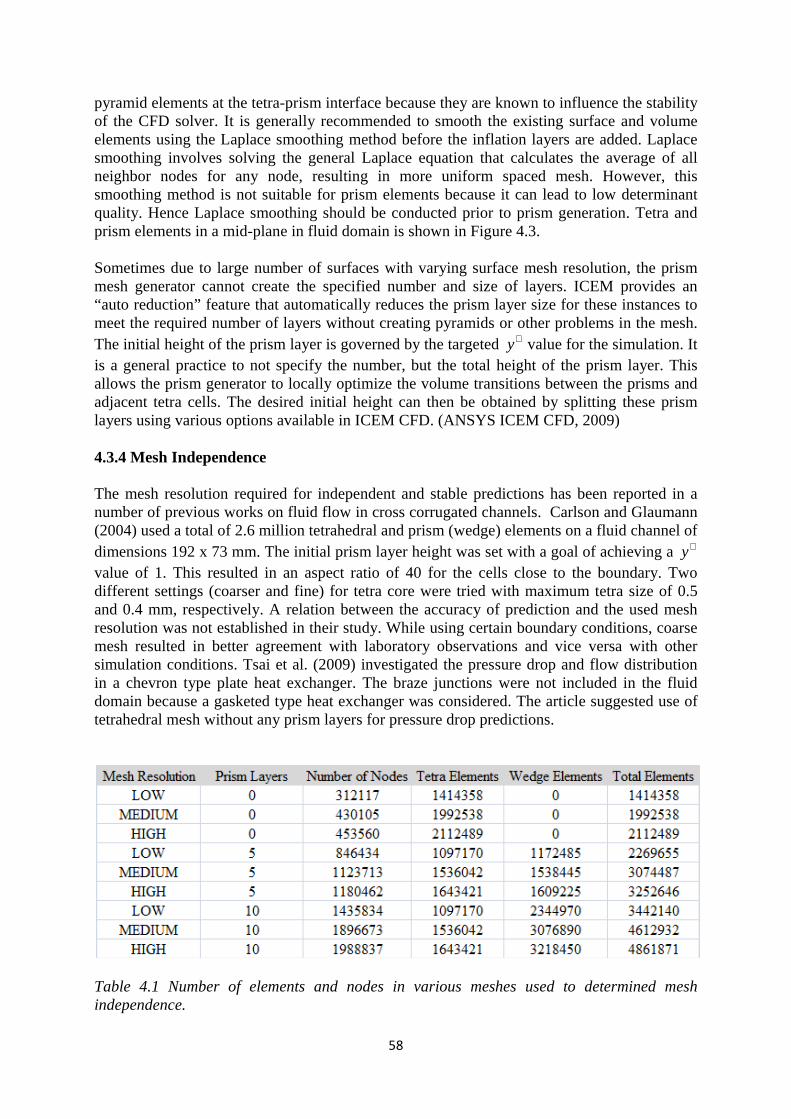
58

pyramid elements at the tetra-prism interface because they are known to influence the stability of the CFD solver. It is generally recommended to smooth the existing surface and volume elements using the Laplace smoothing method before the inflation layers are added. Laplace smoothing involves solving the general Laplace equation that calculates the average of all neighbor nodes for any node, resulting in more uniform spaced mesh. However, this smoothing method is not suitable for prism elements because it can lead to low determinant quality. Hence Laplace smoothing should be conducted prior to prism generation. Tetra and prism elements in a mid-plane in fluid domain is shown in Figure 4.3. Sometimes due to large number of surfaces with varying surface mesh resolution, the prism mesh generator cannot create the specified number and size of layers. ICEM provides an “auto reduction” feature that automatically reduces the prism layer size for these instances to meet the required number of layers without creating pyramids or other problems in the mesh. The initial height of the prism layer is governed by the targeted y+ value for the simulation. It is a general practice to not specify the number, but the total height of the prism layer. This allows the prism generator to locally optimize the volume transitions between the prisms and adjacent tetra cells. The desired initial height can then be obtained by splitting these prism layers using various options available in ICEM CFD. (ANSYS ICEM CFD, 2009) 4.3.4 Mesh Independence The mesh resolution required for independent and stable predictions has been reported in a number of previous works on fluid flow in cross corrugated channels. Carlson and Glaumann (2004) used a total of 2.6 million tetrahedral and prism (wedge) elements on a fluid channel of dimensions 192 x 73 mm. The initial prism layer height was set with a goal of achieving a y+ value of 1. This resulted in an aspect ratio of 40 for the cells close to the boundary. Two different settings (coarser and fine) for tetra core were tried with maximum tetra size of 0.5 and 0.4 mm, respectively. A relation between the accuracy of prediction and the used mesh resolution was not established in their study. While using certain boundary conditions, coarse mesh resulted in better agreement with laboratory observations and vice versa with other simulation conditions. Tsai et al. (2009) investigated the pressure drop and flow distribution in a chevron type plate heat exchanger. The braze junctions were not included in the fluid domain because a gasketed type heat exchanger was considered. The article suggested use of tetrahedral mesh without any prism layers for pressure drop predictions.

Table 4.1 Number of elements and nodes in various meshes used to determined mesh independence.

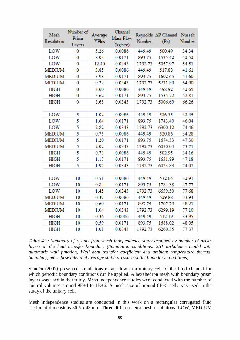
59

Table 4.2: Summary of results from mesh independence study grouped by number of prism layers at the heat transfer boundary (Simulation conditions: SST turbulence model with automatic wall function, Wall heat transfer coefficient and ambient temperature thermal boundary, mass flow inlet and average static pressure outlet boundary conditions) Sundén (2007) presented simulations of air flow in a unitary cell of the fluid channel for which periodic boundary conditions can be applied. A hexahedron mesh with boundary prism layers was used in that study. Mesh independence studies were conducted with the number of control volumes around 9E+4 to 1E+6. A mesh size of around 6E+5 cells was used in the study of the unitary cell. Mesh independence studies are conducted in this work on a rectangular corrugated fluid section of dimensions 80.5 x 43 mm. Three different tetra mesh resolutions (LOW, MEDIUM

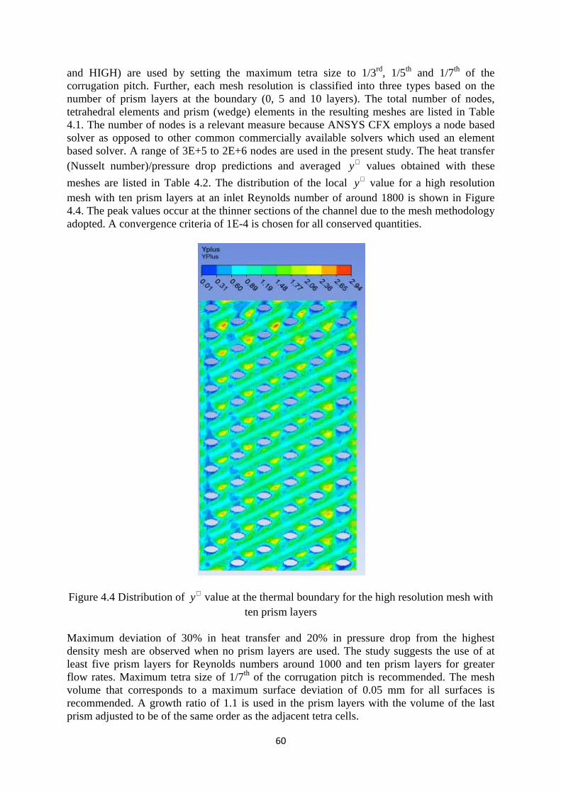
60

and HIGH) are used by setting the maximum tetra size to 1/3rd, 1/5th and 1/7th of the corrugation pitch. Further, each mesh resolution is classified into three types based on the number of prism layers at the boundary (0, 5 and 10 layers). The total number of nodes, tetrahedral elements and prism (wedge) elements in the resulting meshes are listed in Table 4.1. The number of nodes is a relevant measure because ANSYS CFX employs a node based solver as opposed to other common commercially available solvers which used an element based solver. A range of 3E+5 to 2E+6 nodes are used in the present study. The heat transfer (Nusselt number)/pressure drop predictions and averaged y+ values obtained with these

meshes are listed in Table 4.2. The distribution of the local y+ value for a high resolution

mesh with ten prism layers at an inlet Reynolds number of around 1800 is shown in Figure 4.4. The peak values occur at the thinner sections of the channel due to the mesh methodology adopted. A convergence criteria of 1E-4 is chosen for all conserved quantities.

Figure 4.4 Distribution of y+ value at the thermal boundary for the high resolution mesh with ten prism layers

Maximum deviation of 30% in heat transfer and 20% in pressure drop from the highest density mesh are observed when no prism layers are used. The study suggests the use of at least five prism layers for Reynolds numbers around 1000 and ten prism layers for greater flow rates. Maximum tetra size of 1/7th of the corrugation pitch is recommended. The mesh volume that corresponds to a maximum surface deviation of 0.05 mm for all surfaces is recommended. A growth ratio of 1.1 is used in the prism layers with the volume of the last prism adjusted to be of the same order as the adjacent tetra cells.

61

4.4 BOUNDARY CONDITIONS ANSYS CFX 14.0 offers a number of alternative methods to apply wall, inlet and outlet boundary conditions. The choice of the boundary conditions depends on its influence on stability of the simulated case, its influence on the flow conditions within the simulated domain and closeness of representation of the actual application. Computational limitations currently allow for simulation of one or two fluid channels (a single channel for large BPHE models). A study is hence conducted on the influence of wall boundary conditions on the thermal performance prediction for steady-state, incompressible turbulent flow conditions. 4.4.1 Inlet and Outlet The inlet mass flow rate normal to the boundary is specified. A uniform mass flux is assumed and is calculated from the integrated boundary surface for a given mesh resolution according to

s

U m dAρ = ∫ɺ (4.26)

A default turbulence intensity of 0.037 is used, which is an approximate value for internal flow in pipes (ANSYS 2006). The inlet turbulence kinetic energy and dissipation rate are calculated using this intensity. The static inlet temperature is also specified. The average static pressure is specified for the outlet boundary which for a given mesh resolution is found from

spec n

s

P P dA A= ∫ (4.27)

The integrated outlet boundary point pressure is set to the sum of the specified pressure value and the difference between the local node values and the average pressure over the entire boundary. Hence the local pressure profiles can float, but the average value is limited to the specified average static pressure. 4.4.2 Wall Boundary Conditions No slip wall boundary conditions are used for all other surfaces in the fluid domain. The thermal boundary condition can be specified in a variety of ways. Carlson and Glaumann (2004) observed strong dependence of the predicted thermal performance on the specified wall conditions while using the FLUENT 6.1 software. Constant heat flux and constant wall temperature conditions were tried on two fluid channels. The heat transfer in both cases was under-predicted by around 60%. The simulation results were then used to compare the relative performance variation between the two simulated channels. Experimental data suggest a difference of 7.6% between the two models. The constant heat flux condition predicted a difference of 4.6% between the models. The constant temperature boundary conditions predicted a reversed trend with a negative performance variation of -4.2% and was not recommended. The reason for such a strong dependence of the thermal performance on the wall boundary conditions was not discussed in their work. Simulations were conducted in a single fluid section of dimensions 80.5 x 58 mm. The predictions obtained while using various thermal boundary conditions are compared with the

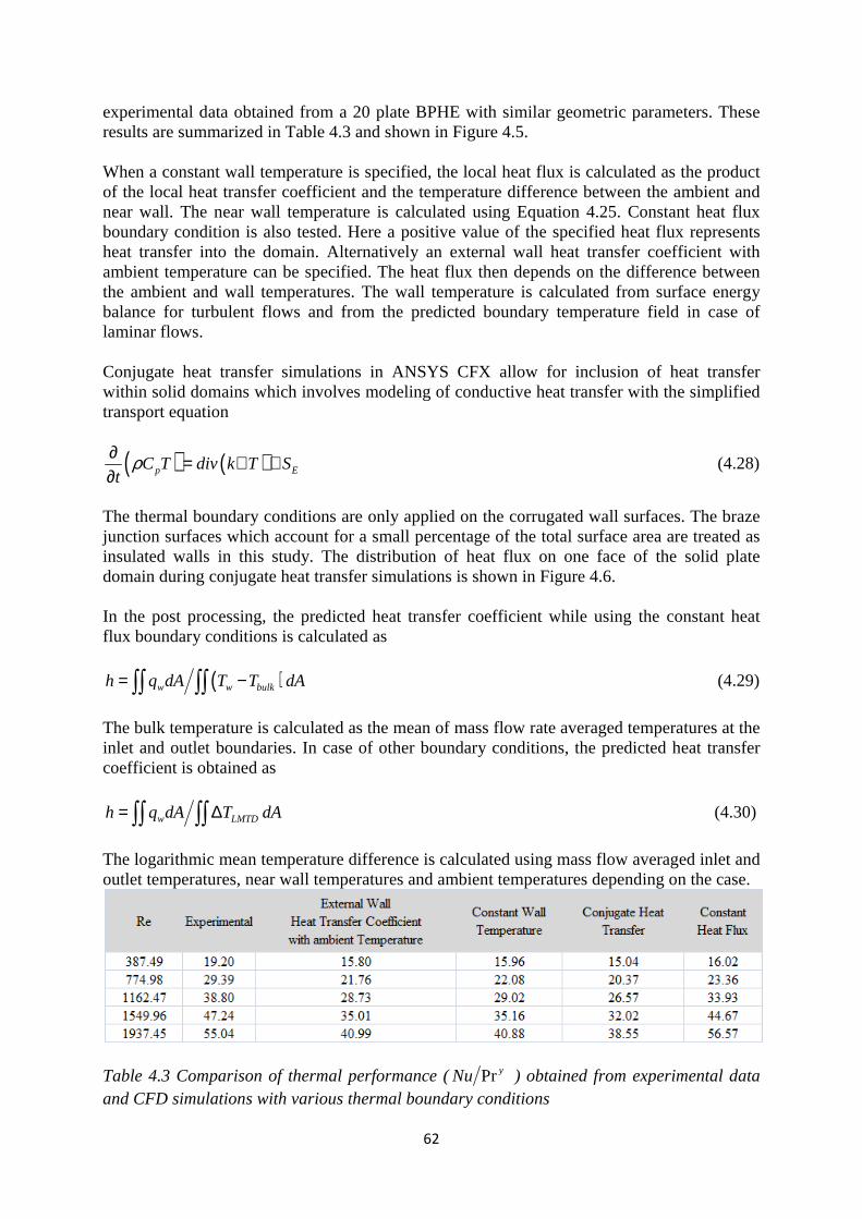
62

experimental data obtained from a 20 plate BPHE with similar geometric parameters. These results are summarized in Table 4.3 and shown in Figure 4.5. When a constant wall temperature is specified, the local heat flux is calculated as the product of the local heat transfer coefficient and the temperature difference between the ambient and near wall. The near wall temperature is calculated using Equation 4.25. Constant heat flux boundary condition is also tested. Here a positive value of the specified heat flux represents heat transfer into the domain. Alternatively an external wall heat transfer coefficient with ambient temperature can be specified. The heat flux then depends on the difference between the ambient and wall temperatures. The wall temperature is calculated from surface energy balance for turbulent flows and from the predicted boundary temperature field in case of laminar flows. Conjugate heat transfer simulations in ANSYS CFX allow for inclusion of heat transfer within solid domains which involves modeling of conductive heat transfer with the simplified transport equation

( ) ( )p EC T div k T St

ρ∂ = ∇ +∂

(4.28)

The thermal boundary conditions are only applied on the corrugated wall surfaces. The braze junction surfaces which account for a small percentage of the total surface area are treated as insulated walls in this study. The distribution of heat flux on one face of the solid plate domain during conjugate heat transfer simulations is shown in Figure 4.6. In the post processing, the predicted heat transfer coefficient while using the constant heat flux boundary conditions is calculated as

( )w w bulkh q dA T T dA= −∫∫ ∫∫ (4.29)

The bulk temperature is calculated as the mean of mass flow rate averaged temperatures at the inlet and outlet boundaries. In case of other boundary conditions, the predicted heat transfer coefficient is obtained as

w LMTDh q dA T dA= ∆∫∫ ∫∫ (4.30)

The logarithmic mean temperature difference is calculated using mass flow averaged inlet and outlet temperatures, near wall temperatures and ambient temperatures depending on the case.

Table 4.3 Comparison of thermal performance (PryNu ) obtained from experimental data and CFD simulations with various thermal boundary conditions

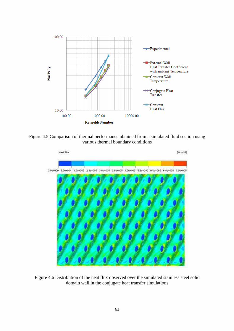
63

Figure 4.5 Comparison of thermal performance obtained from a simulated fluid section using various thermal boundary conditions

Figure 4.6 Distribution of the heat flux observed over the simulated stainless steel solid domain wall in the conjugate heat transfer simulations

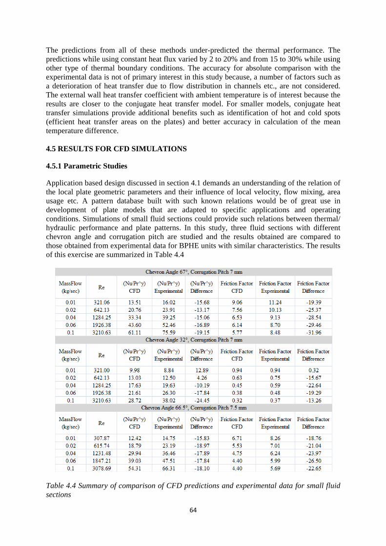
64

The predictions from all of these methods under-predicted the thermal performance. The predictions while using constant heat flux varied by 2 to 20% and from 15 to 30% while using other type of thermal boundary conditions. The accuracy for absolute comparison with the experimental data is not of primary interest in this study because, a number of factors such as a deterioration of heat transfer due to flow distribution in channels etc., are not considered. The external wall heat transfer coefficient with ambient temperature is of interest because the results are closer to the conjugate heat transfer model. For smaller models, conjugate heat transfer simulations provide additional benefits such as identification of hot and cold spots (efficient heat transfer areas on the plates) and better accuracy in calculation of the mean temperature difference. 4.5 RESULTS FOR CFD SIMULATIONS 4.5.1 Parametric Studies Application based design discussed in section 4.1 demands an understanding of the relation of the local plate geometric parameters and their influence of local velocity, flow mixing, area usage etc. A pattern database built with such known relations would be of great use in development of plate models that are adapted to specific applications and operating conditions. Simulations of small fluid sections could provide such relations between thermal/ hydraulic performance and plate patterns. In this study, three fluid sections with different chevron angle and corrugation pitch are studied and the results obtained are compared to those obtained from experimental data for BPHE units with similar characteristics. The results of this exercise are summarized in Table 4.4

Table 4.4 Summary of comparison of CFD predictions and experimental data for small fluid sections

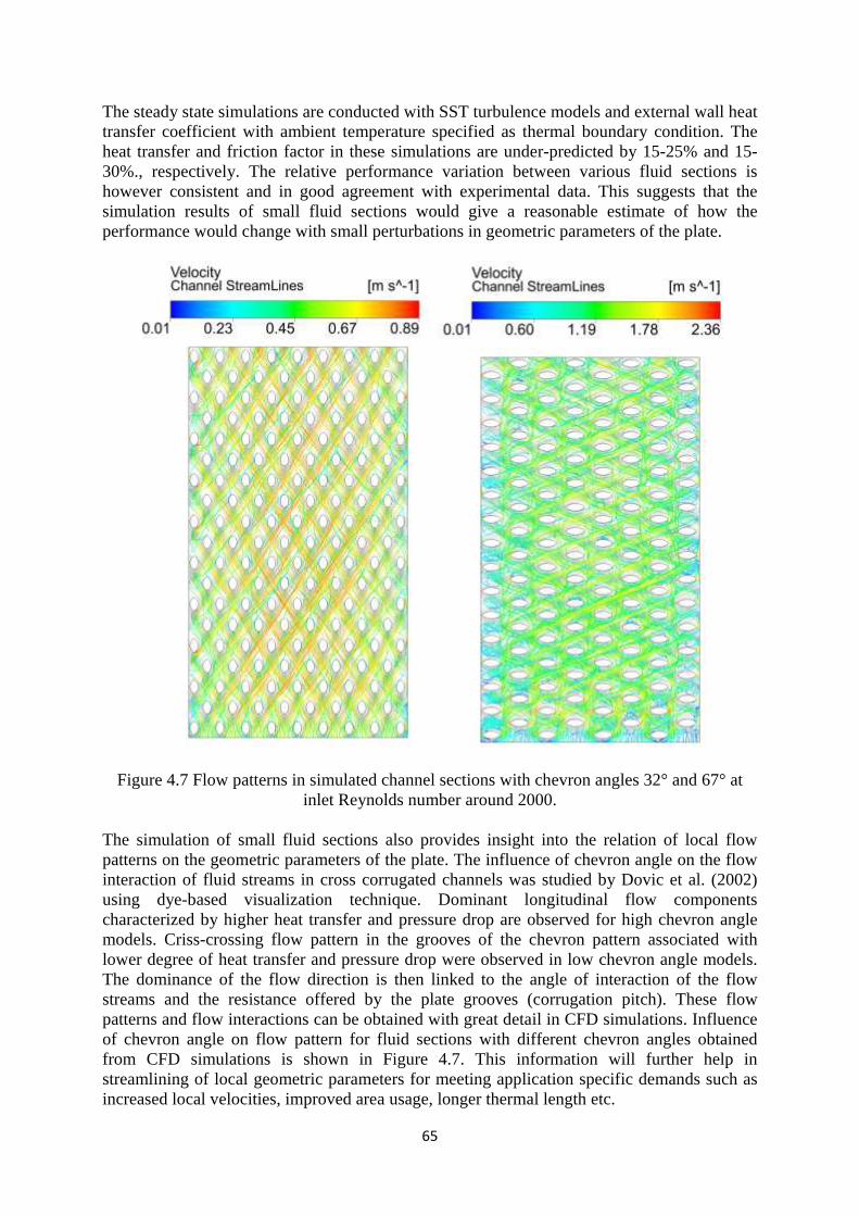
65

The steady state simulations are conducted with SST turbulence models and external wall heat transfer coefficient with ambient temperature specified as thermal boundary condition. The heat transfer and friction factor in these simulations are under-predicted by 15-25% and 15-30%., respectively. The relative performance variation between various fluid sections is however consistent and in good agreement with experimental data. This suggests that the simulation results of small fluid sections would give a reasonable estimate of how the performance would change with small perturbations in geometric parameters of the plate.

Figure 4.7 Flow patterns in simulated channel sections with chevron angles 32° and 67° at inlet Reynolds number around 2000.

The simulation of small fluid sections also provides insight into the relation of local flow patterns on the geometric parameters of the plate. The influence of chevron angle on the flow interaction of fluid streams in cross corrugated channels was studied by Dovic et al. (2002) using dye-based visualization technique. Dominant longitudinal flow components characterized by higher heat transfer and pressure drop are observed for high chevron angle models. Criss-crossing flow pattern in the grooves of the chevron pattern associated with lower degree of heat transfer and pressure drop were observed in low chevron angle models. The dominance of the flow direction is then linked to the angle of interaction of the flow streams and the resistance offered by the plate grooves (corrugation pitch). These flow patterns and flow interactions can be obtained with great detail in CFD simulations. Influence of chevron angle on flow pattern for fluid sections with different chevron angles obtained from CFD simulations is shown in Figure 4.7. This information will further help in streamlining of local geometric parameters for meeting application specific demands such as increased local velocities, improved area usage, longer thermal length etc.

66

4.5.2 Simulation of entire channels The influence of area losses in the distribution region, enhancement of heat transfer due to proprietary design features around ports etc., are not captured in the simulations of smaller fluid sections. Several compensation factors need to be included for thermal and hydraulic correlations obtained from experimental data in order to compare with CFD predictions of smaller fluid sections. For smaller BPHE models, it is of interest to simulate the entire channel to incorporate these additional influences. In this study, a BPHE channel of dimensions 192x73 mm is simulated. The corrugated pattern for this model is characterized by a chevron angle of 65°, corrugation pitch of 7 mm and a pressing depth of 2 mm. Wall heat transfer is modeled using a specified external heat transfer coefficient and ambient temperature. Carlson and Glaumann (2004) conducted simulations of entire channels of similar dimensions using SST turbulence models. The heat transfer predictions in these simulations are sensitive to the wall boundary condition and the thermal performance is under-predicted by 40 to 50%. Tsai et al (2009) conducted pressure drop studies on full channels for gasketed plate heat exchangers. The channel pressure drop was under-predicted by 20% while using the k ε− turbulence model in the Reynolds number range of 600 to 1700. The simulations reported by Sundén (2007) on unitary cells with periodic boundary conditions and a number of different turbulence models over-predicted the heat transfer by as much as 50%. The Fanning fiction factor was under-predicted in most cases. For CFD simulations in this work, an entire fluid channel with approximate braze junction modeling is used. The braze junctions are modeled using three-dimensional fillets with dimensions that are actually measured from cut sections of BPHE models. The mesh recommendations listed in section 4.3 are used and these resulted in a mesh size of around 3.8 million nodes and 11.8 million elements. The mass flow rate at the inlet of the channel is varied to cover a Reynolds number range of 300 to 3000. The results obtained from these simulations and their deviations from experimental observations are summarized in Table 4.5.

Table 4.5 Summary of thermal and hydraulic performance obtained from CFD simulations for entire fluid channel and comparison with experimental data

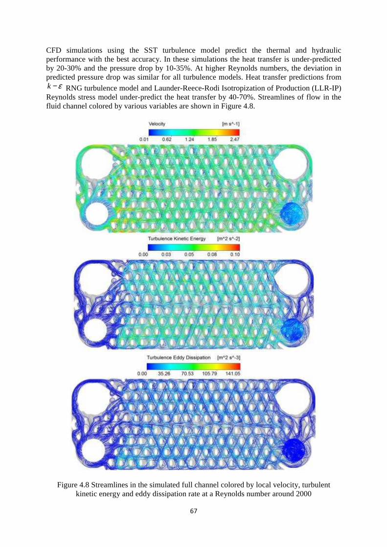
67

CFD simulations using the SST turbulence model predict the thermal and hydraulic performance with the best accuracy. In these simulations the heat transfer is under-predicted by 20-30% and the pressure drop by 10-35%. At higher Reynolds numbers, the deviation in predicted pressure drop was similar for all turbulence models. Heat transfer predictions from k ε− RNG turbulence model and Launder-Reece-Rodi Isotropization of Production (LLR-IP)

Reynolds stress model under-predict the heat transfer by 40-70%. Streamlines of flow in the fluid channel colored by various variables are shown in Figure 4.8.

Figure 4.8 Streamlines in the simulated full channel colored by local velocity, turbulent kinetic energy and eddy dissipation rate at a Reynolds number around 2000

68

4.6 DISCUSSION The governing equations, eddy viscosity based turbulence models, algebraic stress models and various forms of the transport equation are briefly presented. CFD has a major role in design and development of modern application of specific plate patterns. The effectiveness of heat exchangers can be greatly enhanced by optimizing the local geometric parameters and further improvements made to existing plate features. Simulations on small fluid sections provide an excellent indication of performance variation and flow physics with respect to geometric parameters. For larger models, computational limitations restrict use of single fluid domain and approximate thermal boundary conditions. Conjugate heat transfer simulations provide benefits such as accurate determination of mean temperature difference, identification of efficient heat transfer areas on the plate and comparison of flow patterns in alternate channels. The SST turbulence model combined with specified external wall heat transfer coefficient and ambient temperature predicted the pressure drop and heat transfer with reasonable accuracy. Some of the variation in predictions can be attributed to the approximate modeling of the braze junctions in the fluid domain. LES and DES simulations are not considered in this study due to hardware limitations but are of great interest for further research. Further studies are also required to calibrate quantities such as inlet turbulence intensity and empirical constants in the transport equations for turbulence terms. REFERENCES ANSYS Inc., ANSYS CFX-Solver Theory Guide, ANSYS CFX Release 11.0, December 2006 ANSYS Inc., ANSYS ICEM CFD Tutorial Manual, 2009 Carlson, A., and Glaumann, J., Simulation of heat transfer in compact brazed plate heat exchangers using CFD software Fluent, Master Thesis, Lund University, ISRN LUTMDN/TMHP-04/5034-SE ISSN 0282-1990, 2004 Dovic, D., Palm, B., and Svaic, S., Basic single-phase flow phenomena in chevron-type plate heat exchangers, Zero Leakage – Minimum Charge, IIR/IIF, Stockholm, pp. 221-232, 2002 Schlichting, H., and Gersten, K., Boundary Layer Theory, 8th revised edition, Springer, ISBN 3-540-66270-7, 2000 Sjögren, T., Development and validation of turbulence models through experiment and computation, Doctoral Thesis, Royal Institute of Technology, Sweden, ISRN KTH/MEK/TR—97/5—SE, 1997 Sundén, B., Computational fluid dynamics in research and design of heat exchangers, Heat Transfer Engineering, Volume 28, No 11, pp. 898-910, 2007 Tsai, Y.C., Liu, F.B., and Shen, P.T., Investigations of the pressure drop and flow distribution in a chevron-type plate heat exchanger, International Communication in Heat and Mass Transfer 36: pp. 574-578, 2009

69

5.0 RESULTS – PERFORMANCE

ANALYSIS

The suitability of employing a generalized pressure-enthalpy based step wise rating method for performance analysis and design of brazed plate heat exchangers is presented in this chapter. Generalized thermal and hydraulic correlations derived for various applications are also listed. The influence of geometric parameters and flow configurations on the performance predictions is briefly mentioned. The influence of measurement techniques and correlations evaluation methodology employed on the reliability of the BPHE calculation software is also discussed.

5.1 INTRODUCTION Reliability and scalability are the principal desirable characteristics for heat exchanger selection software. These characteristics depend on the quality and scalability of the thermal and hydraulic correlations used in the design process. Product specific thermal and hydraulic correlations usually offer better reliability as compared to generalized correlations for performance scaling and prediction of off-test conditions. Generalized correlations for thermal and hydraulic behavior of brazed plate heat exchangers in the literature are often limited by lack of generality in definition of geometric parameters, limited test range, variation in calculation methodologies and other uncertainties posed by the manufacturer specific production processes and design features. The correlations in the literature, however, highlight the influence of various factors on BPHE performance and outline ideas employed by various investigators for tackling them. These could be in the form of rule of thumb or correction factors that can be applied to base thermal and hydraulic correlations. Generalized correlations are however important for prediction of performance of new designs aiming at new applications and broadened operation envelopes involving non conventional process fluids and often, more stringent design constraints. The developed generalized pressure-enthalpy based rating method is used as the basis for the development of such generalized correlations. The generalized correlations are developed as functions of flow arrangement and configurations, local fluid properties, geometric properties and standard non-dimensional numbers. The benefits and limitations of the developed calculation procedure for various applications such as transcritical gas cooling, condensing, evaporating, cascaded heat transfer etc., are outlined. From the information generated from the discretized calculations, further design constraints and solutions for handling them and listed for several applications. The measurement data adopted in this study is based on several single phase and phase change tests conducted at SWEP International AB. A brief description of the measurement rig and uncertainty estimation is presented for various applications. The testing methodology that needs to be adopted to overcome the numerical errors while using standard test data evaluation methods is presented. Furthermore, the use of the developed correlations and outcome of the studies in Chapter 4 in designing BPHEs for new applications is briefly discussed.

70

5.2 SINGLE PHASE TESTING The generalized correlations derived and the method development carried out in this thesis work is based on the experimental data obtained from SWEP International AB. Product specific single phase thermal and hydraulic correlations are derived for all BPHE models based on tests using Water and Water/Glycerin mixture. These correlations are also used to model convective heat transfer and friction pressure drop in phase change calculations. BPHE test objects are chosen so that a wide range of channel flow Reynolds number is covered from a possible mass flow range of 0.4 to 10 kg/s. Temperatures on the cold side usually vary from 20-40°C and those on hot side from 50 to 65°C. For smaller BPHE models it is often required to utilize parallel connected BPHE units for obtaining correlations at low flow conditions. The sensors used are periodically calibrated. The test program is generated by randomly varying inlet temperatures and flow rates in order to eliminate hysteresis errors. Temperature measurements are conducted using resistance type PT-100 sensors with a tolerance of ±0.1 K. Measurements were conducted two meters away from the ports and static mixer is used on the outlet port to achieve temperature stabilization for high viscous fluids. Rosemount differential pressure sensors with a tolerance of ±0.025% in the entire span are used for pressure drop measurement. Coriolis type mass flow meter with a maximum tolerance of ±0.2% is used for mass flow measurement on the cold side. An inductive type volume flow meter with a tolerance of ±0.25% is used for flow measurement on the warm side. Test data from water tests are used for correlation evaluation in the Reynolds number range of around 600 to 10000 and the data from water/glycerin mixture is used for the Reynolds number range of 10 to 300. The performance in a small intermediate portion of the Reynolds number range is usually interpolated. For symmetric heat exchangers (those with similar channel characteristic on the primary and secondary side), two tests are sufficient to generate correlations for the entire Reynolds number range. For asymmetric models (those with significant performance variation in the primary and secondary channels), three tests are required for generating channel specific correlations. The high and low Reynolds number region tests usually yield 30 test points which are further filtered based on additional criteria such as energy balance, minimum temperature difference and the measured values being in the range of the measurement equipment. Test points with a minimum temperature difference lower than 3K are associated with relatively high uncertainty in data reduction stage and hence not used. The data reduction is performed using the methods outlined in section 2.2 for the correlation evaluation and involves determination of the empirical constants in the equations 2.10 and 2.11. The worst case uncertainty of a derived quantity R which is a function of n measure quantities ( )1 2 3, , .... nx x x x is determined

as follows. (Moffat 1982)

( )1 2 3, , .... nR R x x x x≡ (5.1)

1 21 2

...... nn

R R RR x x x

x x xδ δ δ δ∂ ∂ ∂= + + +

∂ ∂ ∂ (5.2)

For the specified uncertainties in temperature, differential pressure and flow rate measurements and the criteria employed in qualifying the validity of test points, the maximum uncertainty in the prediction of overall heat transfer coefficient is calculated to be less than 1%. Data evaluation is conducted using the modified Wilson plot method with combination of direct search algorithms as elaborated in section 3.5.

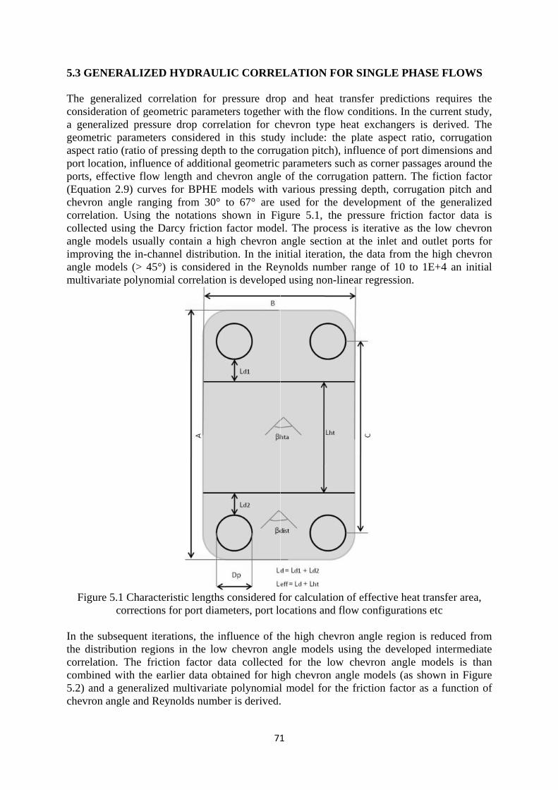
5.3 GENERALIZED HYDR The generalized correlation for pressure drop and heat transfer predictions requires the consideration of geometric parameters together with the flow conditions. In the current study, a generalized pressure drop geometric parameters considered in this study include: the plate aspect ratio, corrugation aspect ratio (ratio of pressing depth to the corrugation pitch), influence of port dimensions and port location, influence of additional geometric parameters such as corner passages around the ports, effective flow length and chevron angle of the corrugation pattern. The fiction factor (Equation 2.9) curves for BPHE models with various pressing depth, corrugchevron angle ranging from 30° to 67° are used for the development of the generalized correlation. Using the notations shown in Figure 5.collected using the Darcy friction factor angle models usually contain a high chevron angle section at the inlet and outlet ports for improving the inangle models (> 45°) is considered in multivariate polynomial correlation is developed using non

Figure 5.1 Characteristic lengths considered for calculation of effective heat transfer area, corrections for port diameters

In the subsequent iterations, the influence of the high chevron angle region is reduced from the distribution regions in the low chevron angle models using the developed intermediate correlation. The friction combined with the earlier data obtained for high chevron angle models (as shown in 5.2) and a generalized multivariate polynomial model for chevron angle and Reynolds number is derived.

71

GENERALIZED HYDR AULIC CORRELATION FOR SINGLE PHASE FLOWS

The generalized correlation for pressure drop and heat transfer predictions requires the consideration of geometric parameters together with the flow conditions. In the current study, a generalized pressure drop correlation for chevron type heat exchangers is derived. The geometric parameters considered in this study include: the plate aspect ratio, corrugation aspect ratio (ratio of pressing depth to the corrugation pitch), influence of port dimensions and

ocation, influence of additional geometric parameters such as corner passages around the ports, effective flow length and chevron angle of the corrugation pattern. The fiction factor (Equation 2.9) curves for BPHE models with various pressing depth, corrugchevron angle ranging from 30° to 67° are used for the development of the generalized

Using the notations shown in Figure 5.collected using the Darcy friction factor model. Theangle models usually contain a high chevron angle section at the inlet and outlet ports for improving the in-channel distribution. In the initial iteration, the data from the high chevron angle models (> 45°) is considered in the Reynolds number range of 10 to 1E+4 an initial multivariate polynomial correlation is developed using non

Characteristic lengths considered for calculation of effective heat transfer area, corrections for port diameters, port locations and flow configurations etc

In the subsequent iterations, the influence of the high chevron angle region is reduced from the distribution regions in the low chevron angle models using the developed intermediate correlation. The friction factor data collected for the low chevron angle models is than combined with the earlier data obtained for high chevron angle models (as shown in

) and a generalized multivariate polynomial model for ngle and Reynolds number is derived.

71

AULIC CORRELATION FOR SINGLE PHASE FLOWS

The generalized correlation for pressure drop and heat transfer predictions requires the consideration of geometric parameters together with the flow conditions. In the current study,

correlation for chevron type heat exchangers is derived. The geometric parameters considered in this study include: the plate aspect ratio, corrugation aspect ratio (ratio of pressing depth to the corrugation pitch), influence of port dimensions and

ocation, influence of additional geometric parameters such as corner passages around the ports, effective flow length and chevron angle of the corrugation pattern. The fiction factor (Equation 2.9) curves for BPHE models with various pressing depth, corrugchevron angle ranging from 30° to 67° are used for the development of the generalized

Using the notations shown in Figure 5.1, the pressure friction factor data is model. The process is iterative as the low chevron

angle models usually contain a high chevron angle section at the inlet and outlet ports for channel distribution. In the initial iteration, the data from the high chevron

the Reynolds number range of 10 to 1E+4 an initial multivariate polynomial correlation is developed using non-linear regression.

Characteristic lengths considered for calculation of effective heat transfer area,

, port locations and flow configurations etc

In the subsequent iterations, the influence of the high chevron angle region is reduced from the distribution regions in the low chevron angle models using the developed intermediate

factor data collected for the low chevron angle models is than combined with the earlier data obtained for high chevron angle models (as shown in

) and a generalized multivariate polynomial model for the friction factor as a function of ngle and Reynolds number is derived.

AULIC CORRELATION FOR SINGLE PHASE FLOWS

The generalized correlation for pressure drop and heat transfer predictions requires the consideration of geometric parameters together with the flow conditions. In the current study,

correlation for chevron type heat exchangers is derived. The geometric parameters considered in this study include: the plate aspect ratio, corrugation aspect ratio (ratio of pressing depth to the corrugation pitch), influence of port dimensions and

ocation, influence of additional geometric parameters such as corner passages around the ports, effective flow length and chevron angle of the corrugation pattern. The fiction factor (Equation 2.9) curves for BPHE models with various pressing depth, corrugation pitch and chevron angle ranging from 30° to 67° are used for the development of the generalized

, the pressure friction factor data is the low chevron

angle models usually contain a high chevron angle section at the inlet and outlet ports for channel distribution. In the initial iteration, the data from the high chevron

the Reynolds number range of 10 to 1E+4 an initial

Characteristic lengths considered for calculation of effective heat transfer area, , port locations and flow configurations etc

In the subsequent iterations, the influence of the high chevron angle region is reduced from the distribution regions in the low chevron angle models using the developed intermediate

factor data collected for the low chevron angle models is than combined with the earlier data obtained for high chevron angle models (as shown in Figure

friction factor as a function of

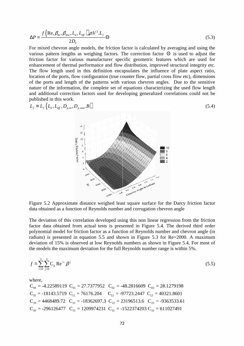
(Re, , , , . . .ht dist d eff ff L L V LP

β β ρ∆ = Θ

For mixed chevron angle models, the friction factor is calculated by averagingvarious pattern lengths as weighing factors. The correction factor friction factor for various manufacturer specific geometric features enhancement of thermal performance and flow distribution, improved structural integrity etc. The flow length used in thilocation of the ports, flow configuration (true counter flow, partial cross flow etc), dimensions of the ports and length of the patterns with various chevron angles. Due to the sensitive nature of the information, the complete set of equations characterizing the used flow length and additional correction factors used for developing generalized correlations could not be published in this work.

( , , , .f f d eff p in p ioutL L L L D D B≡

Figure 5.2 Approximate distance weighed least square surface for the Darcy friction factor data obtained as a function of Reynolds number and corrugation chevron angle The deviation of this correlation developed using this non linear regression from the factor data obtained from actual tests is presented in Figure 5.4. polynomial model for friction factor as a function of Reynolds number and chevron angle (in radians) is presented in equation 5.deviation of 15% is observed at low Reynolds numbersthe models the maximum deviation for the full Reynolds number range is within 5%.

3 3

0 0

C Reiji j

f= =

=∑∑

where,

00 01 02 03

10 11 12 13

20 21 22

C = -4.22589119 C = 27.7377952 C = -4

C = -18143.5719 C = 76176.204 C = -

C = 4468489.72 C = -18362697.3 C = 23

30 31 32 33C = -296126477 C = 1209974231 C = -15

72

) 2Re, , , , . . .

2ht dist d eff f

h

f L L V L

D

β β ρ∆ = Θ

For mixed chevron angle models, the friction factor is calculated by averagingvarious pattern lengths as weighing factors. The correction factor friction factor for various manufacturer specific geometric features enhancement of thermal performance and flow distribution, improved structural integrity etc. The flow length used in this definition encapsulates the influence of plate aspect ratio, location of the ports, flow configuration (true counter flow, partial cross flow etc), dimensions of the ports and length of the patterns with various chevron angles. Due to the sensitive

re of the information, the complete set of equations characterizing the used flow length and additional correction factors used for developing generalized correlations could not be published in this work.

), ,, , , .f f d eff p in p ioutL L L L D D B

Approximate distance weighed least square surface for the Darcy friction factor data obtained as a function of Reynolds number and corrugation chevron angle

The deviation of this correlation developed using this non linear regression from the factor data obtained from actual tests is presented in Figure 5.4. polynomial model for friction factor as a function of Reynolds number and chevron angle (in

ns) is presented in equation 5.5 and shown in Figure 5.3 fodeviation of 15% is observed at low Reynolds numbersthe models the maximum deviation for the full Reynolds number range is within 5%.

C Re i jβ−

00 01 02 03

10 11 12 13

20 21 22

C = -4.22589119 C = 27.7377952 C = -4

C = -18143.5719 C = 76176.204 C = -97723.2447 C = 40321.8601

C = 4468489.72 C = -18362697.3 C = 23

30 31 32 33C = -296126477 C = 1209974231 C = -15

72

For mixed chevron angle models, the friction factor is calculated by averagingvarious pattern lengths as weighing factors. The correction factor Θ is used to adjust the friction factor for various manufacturer specific geometric features which are enhancement of thermal performance and flow distribution, improved structural integrity etc.

s definition encapsulates the influence of plate aspect ratio, location of the ports, flow configuration (true counter flow, partial cross flow etc), dimensions of the ports and length of the patterns with various chevron angles. Due to the sensitive

re of the information, the complete set of equations characterizing the used flow length and additional correction factors used for developing generalized correlations could not be

Approximate distance weighed least square surface for the Darcy friction factor

data obtained as a function of Reynolds number and corrugation chevron angle

The deviation of this correlation developed using this non linear regression from the factor data obtained from actual tests is presented in Figure 5.4. The derived third order polynomial model for friction factor as a function of Reynolds number and chevron angle (in

5 and shown in Figure 5.3 for Re=2000.deviation of 15% is observed at low Reynolds numbers as shown in Figure 5.the models the maximum deviation for the full Reynolds number range is within 5%.

00 01 02 03

10 11 12 13

C = -4.22589119 C = 27.7377952 C = -48.2816609 C = 28.1279198

C = -18143.5719 C = 76176.204 C = -97723.2447 C = 40321.8601

C = 4468489.72 C = -18362697.3 C = 23196513. 23

30 31 32 33

6 C = -9363533.61

C = -296126477 C = 1209974231 C = -1522374203 C = 611027491

(5.3)

For mixed chevron angle models, the friction factor is calculated by averaging and using the is used to adjust the which are used for

enhancement of thermal performance and flow distribution, improved structural integrity etc. s definition encapsulates the influence of plate aspect ratio,

location of the ports, flow configuration (true counter flow, partial cross flow etc), dimensions of the ports and length of the patterns with various chevron angles. Due to the sensitive

re of the information, the complete set of equations characterizing the used flow length and additional correction factors used for developing generalized correlations could not be

(5.4)

Approximate distance weighed least square surface for the Darcy friction factor data obtained as a function of Reynolds number and corrugation chevron angle

The deviation of this correlation developed using this non linear regression from the friction The derived third order

polynomial model for friction factor as a function of Reynolds number and chevron angle (in r Re=2000. A maximum

as shown in Figure 5.4. For most of the models the maximum deviation for the full Reynolds number range is within 5%.

(5.5)

8.2816609 C = 28.1279198

97723.2447 C = 40321.8601

6 C = -9363533.61

22374203 C = 611027491

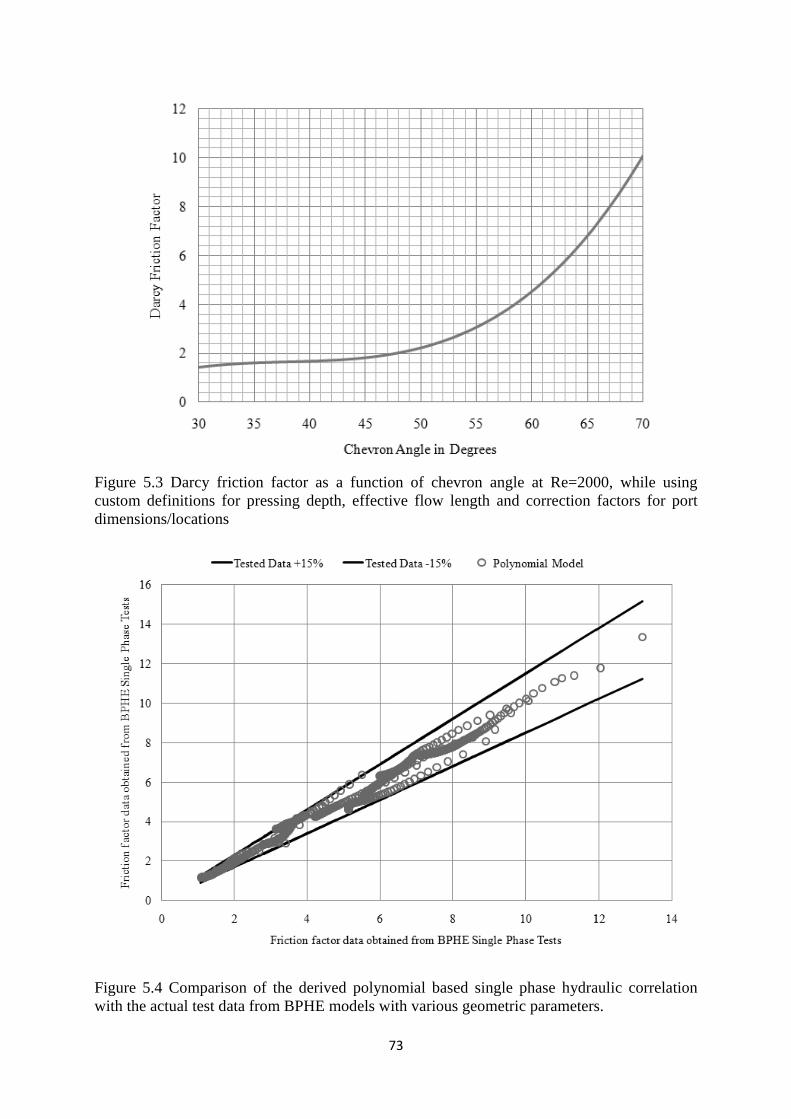
Figure 5.3 Darcy friction factor custom definitions for pressing depth, effective flow length and correctidimensions/locations

Figure 5.4 Comparison of the derived polynomial based single phase hydraulic correlation with the actual test data from BPHE models with various geometric parameters.

73

Darcy friction factor as a function of chevron angle at Re=2000, while using custom definitions for pressing depth, effective flow length and correcti

locations

Comparison of the derived polynomial based single phase hydraulic correlation with the actual test data from BPHE models with various geometric parameters.

73

a function of chevron angle at Re=2000, while using custom definitions for pressing depth, effective flow length and correction factors for port

Comparison of the derived polynomial based single phase hydraulic correlation with the actual test data from BPHE models with various geometric parameters.

a function of chevron angle at Re=2000, while using

on factors for port

Comparison of the derived polynomial based single phase hydraulic correlation with the actual test data from BPHE models with various geometric parameters.

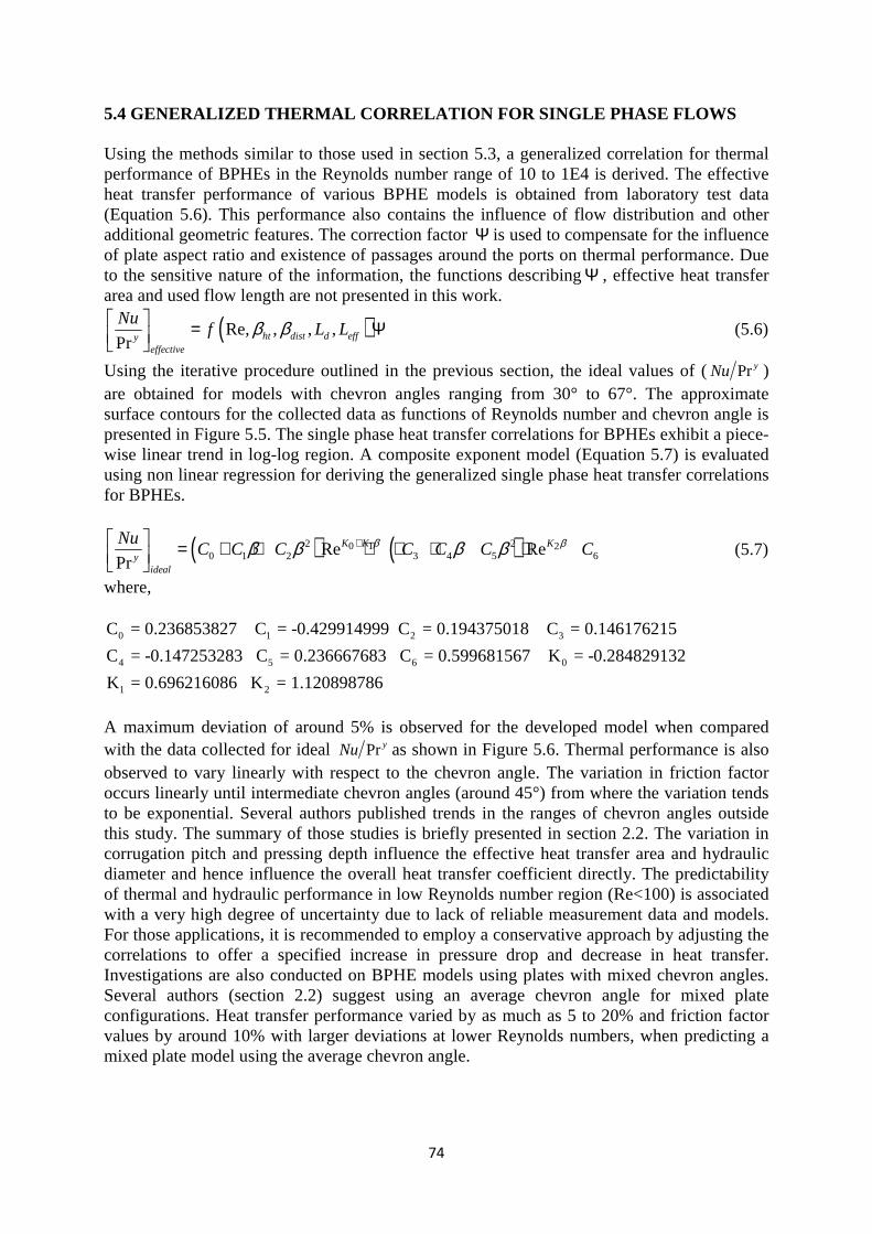
74

5.4 GENERALIZED THERMAL CORRELATION FOR SINGLE PHASE FLOWS Using the methods similar to those used in section 5.3, a generalized correlation for thermal performance of BPHEs in the Reynolds number range of 10 to 1E4 is derived. The effective heat transfer performance of various BPHE models is obtained from laboratory test data (Equation 5.6). This performance also contains the influence of flow distribution and other additional geometric features. The correction factor Ψ is used to compensate for the influence of plate aspect ratio and existence of passages around the ports on thermal performance. Due to the sensitive nature of the information, the functions describingΨ , effective heat transfer area and used flow length are not presented in this work.

( )Re, , , ,Pr ht dist d effy

effective

Nuf L Lβ β = Ψ

(5.6)

Using the iterative procedure outlined in the previous section, the ideal values of ( PryNu ) are obtained for models with chevron angles ranging from 30° to 67°. The approximate surface contours for the collected data as functions of Reynolds number and chevron angle is presented in Figure 5.5. The single phase heat transfer correlations for BPHEs exhibit a piece- wise linear trend in log-log region. A composite exponent model (Equation 5.7) is evaluated using non linear regression for deriving the generalized single phase heat transfer correlations for BPHEs.

( ) ( )2 20 1 20 1 2 3 4 5 6Re Re

PrK K K

yideal

NuC C C C C C Cβ ββ β β β+ = + + + + + +

(5.7)

where,

0 1 2 3

4 5 6 0

1 2

C = 0.236853827 C = -0.429914999 C = 0.194375018 C = 0.146176215

C = -0.147253283 C = 0.236667683 C = 0.599681567 K = -0.284829132

K = 0.696216086 K = 1.120898786

A maximum deviation of around 5% is observed for the developed model when compared with the data collected for ideal PryNu as shown in Figure 5.6. Thermal performance is also observed to vary linearly with respect to the chevron angle. The variation in friction factor occurs linearly until intermediate chevron angles (around 45°) from where the variation tends to be exponential. Several authors published trends in the ranges of chevron angles outside this study. The summary of those studies is briefly presented in section 2.2. The variation in corrugation pitch and pressing depth influence the effective heat transfer area and hydraulic diameter and hence influence the overall heat transfer coefficient directly. The predictability of thermal and hydraulic performance in low Reynolds number region (Re<100) is associated with a very high degree of uncertainty due to lack of reliable measurement data and models. For those applications, it is recommended to employ a conservative approach by adjusting the correlations to offer a specified increase in pressure drop and decrease in heat transfer. Investigations are also conducted on BPHE models using plates with mixed chevron angles. Several authors (section 2.2) suggest using an average chevron angle for mixed plate configurations. Heat transfer performance varied by as much as 5 to 20% and friction factor values by around 10% with larger deviations at lower Reynolds numbers, when predicting a mixed plate model using the average chevron angle.

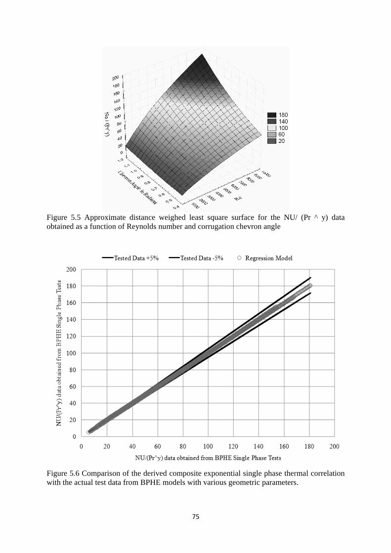
Figure 5.5 Approximate distance weighed least square surface for the NU/ (Pr ^ y) data obtained as a function of Reynolds number and corrugation chevron angle

Figure 5.6 Comparison of the derived composite exponential single phase thermal correlation with the actual test data from BPHE models with various geometric parameters.

75

Approximate distance weighed least square surface for the NU/ (Pr ^ y) data obtained as a function of Reynolds number and corrugation chevron angle

Comparison of the derived composite exponential single phase thermal correlation with the actual test data from BPHE models with various geometric parameters.

75

Approximate distance weighed least square surface for the NU/ (Pr ^ y) data

obtained as a function of Reynolds number and corrugation chevron angle

Comparison of the derived composite exponential single phase thermal correlation with the actual test data from BPHE models with various geometric parameters.

Approximate distance weighed least square surface for the NU/ (Pr ^ y) data

Comparison of the derived composite exponential single phase thermal correlation

with the actual test data from BPHE models with various geometric parameters.

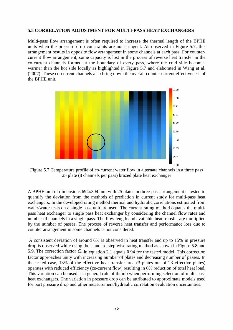
76

5.5 CORRELATION ADJUSTMENT FOR MULTI-PASS HEAT EXCHANGERS

Multi-pass flow arrangement is often required to increase the thermal length of the BPHE units when the pressure drop constraints are not stringent. As observed in Figure 5.7, this arrangement results in opposite flow arrangement in some channels at each pass. For counter-current flow arrangement, some capacity is lost in the process of reverse heat transfer in the co-current channels formed at the boundary of every pass, where the cold side becomes warmer than the hot side locally as highlighted in Figure 5.7 and elaborated in Wang et al. (2007). These co-current channels also bring down the overall counter current effectiveness of the BPHE unit.

Figure 5.7 Temperature profile of co-current water flow in alternate channels in a three pass

25 plate (8 channels per pass) brazed plate heat exchanger A BPHE unit of dimensions 694x304 mm with 25 plates in three-pass arrangement is tested to quantify the deviation from the methods of prediction in current study for multi-pass heat exchangers. In the developed rating method thermal and hydraulic correlations estimated from water/water tests on a single pass unit are used. The current rating method equates the multi-pass heat exchanger to single pass heat exchanger by considering the channel flow rates and number of channels in a single pass. The flow length and available heat transfer are multiplied by the number of passes. The process of reverse heat transfer and performance loss due to counter arrangement in some channels is not considered. A consistent deviation of around 6% is observed in heat transfer and up to 15% in pressure drop is observed while using the standard step wise rating method as shown in Figure 5.8 and 5.9. The correction factor Ω in equation 2.1 equals 0.94 for the tested model. This correction factor approaches unity with increasing number of plates and decreasing number of passes. In the tested case, 13% of the effective heat transfer area (3 plates out of 23 effective plates) operates with reduced efficiency (co-current flow) resulting in 6% reduction of total heat load. This variation can be used as a general rule of thumb when performing selection of multi-pass heat exchangers. The variation in pressure drop can be attributed to approximate models used for port pressure drop and other measurement/hydraulic correlation evaluation uncertainties.

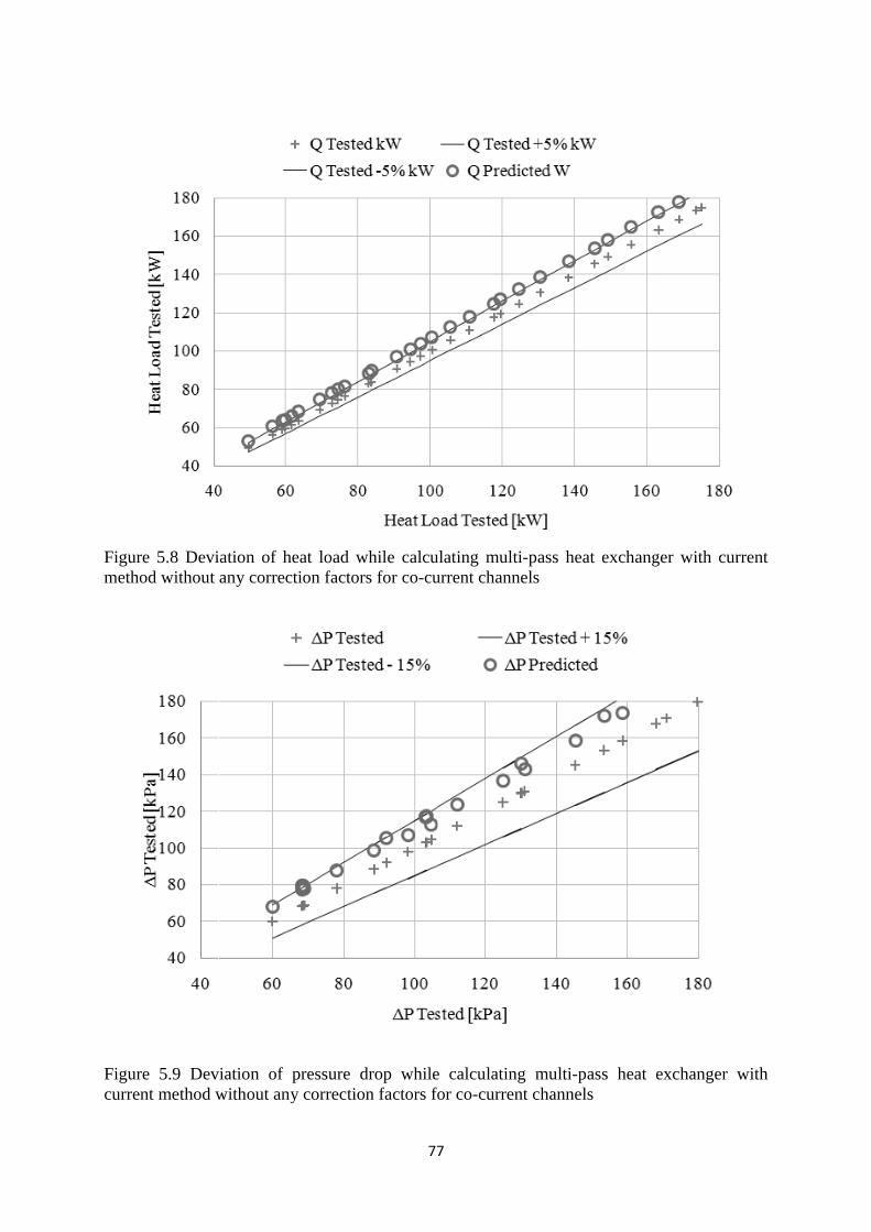
Figure 5.8 Deviation of heat load while calculating multimethod without any correction factors f

Figure 5.9 Deviation of pressure drop while calculating multicurrent method without any correction factors for co

77

Deviation of heat load while calculating multimethod without any correction factors for co-current channels

Deviation of pressure drop while calculating multicurrent method without any correction factors for co

77

Deviation of heat load while calculating multi-pass heat exchanger with current current channels

Deviation of pressure drop while calculating multi-pass heat exchanger with current method without any correction factors for co-current channels

pass heat exchanger with current

pass heat exchanger with

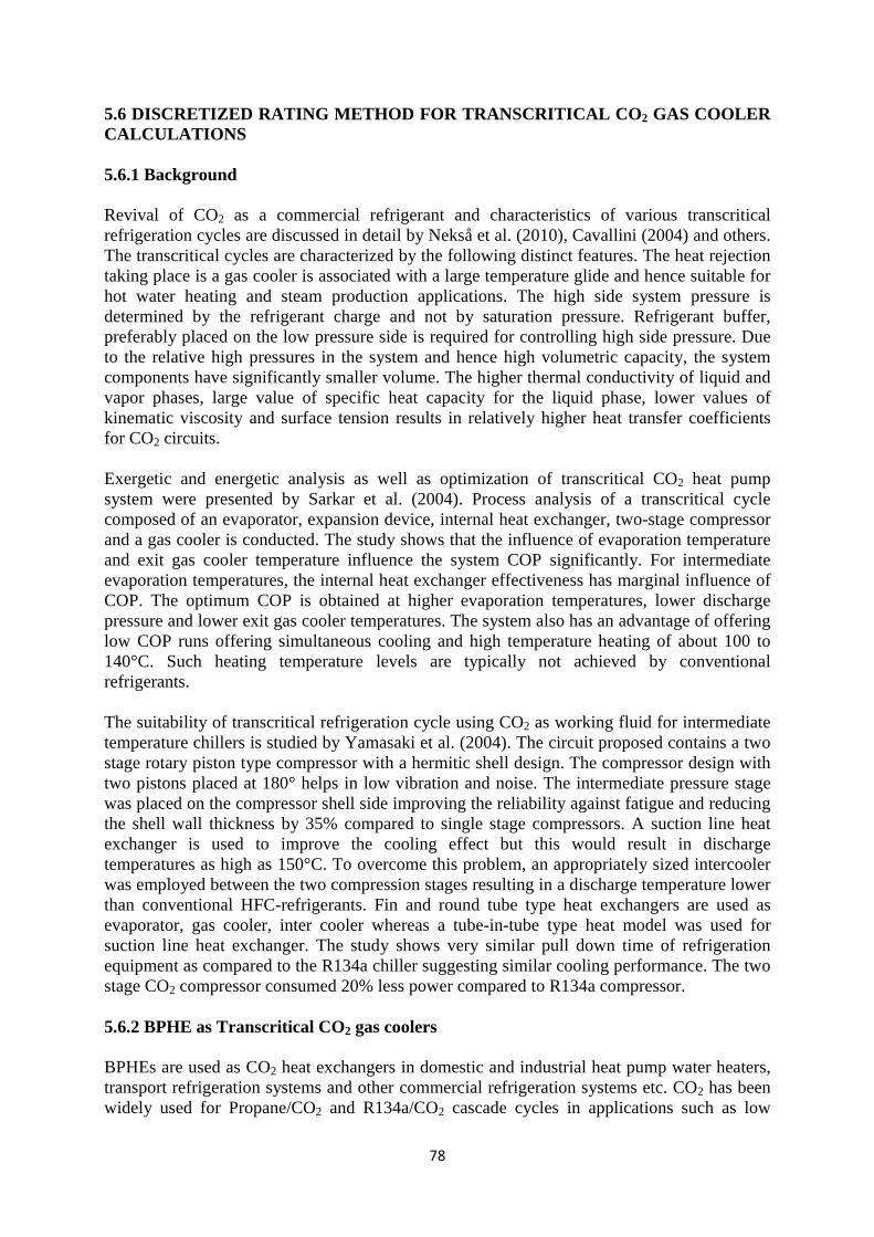
78

5.6 DISCRETIZED RATING METHOD FOR TRANSCRITICAL CO 2 GAS COOLER CALCULATIONS 5.6.1 Background Revival of CO2 as a commercial refrigerant and characteristics of various transcritical refrigeration cycles are discussed in detail by Nekså et al. (2010), Cavallini (2004) and others. The transcritical cycles are characterized by the following distinct features. The heat rejection taking place is a gas cooler is associated with a large temperature glide and hence suitable for hot water heating and steam production applications. The high side system pressure is determined by the refrigerant charge and not by saturation pressure. Refrigerant buffer, preferably placed on the low pressure side is required for controlling high side pressure. Due to the relative high pressures in the system and hence high volumetric capacity, the system components have significantly smaller volume. The higher thermal conductivity of liquid and vapor phases, large value of specific heat capacity for the liquid phase, lower values of kinematic viscosity and surface tension results in relatively higher heat transfer coefficients for CO2 circuits. Exergetic and energetic analysis as well as optimization of transcritical CO2 heat pump system were presented by Sarkar et al. (2004). Process analysis of a transcritical cycle composed of an evaporator, expansion device, internal heat exchanger, two-stage compressor and a gas cooler is conducted. The study shows that the influence of evaporation temperature and exit gas cooler temperature influence the system COP significantly. For intermediate evaporation temperatures, the internal heat exchanger effectiveness has marginal influence of COP. The optimum COP is obtained at higher evaporation temperatures, lower discharge pressure and lower exit gas cooler temperatures. The system also has an advantage of offering low COP runs offering simultaneous cooling and high temperature heating of about 100 to 140°C. Such heating temperature levels are typically not achieved by conventional refrigerants. The suitability of transcritical refrigeration cycle using CO2 as working fluid for intermediate temperature chillers is studied by Yamasaki et al. (2004). The circuit proposed contains a two stage rotary piston type compressor with a hermitic shell design. The compressor design with two pistons placed at 180° helps in low vibration and noise. The intermediate pressure stage was placed on the compressor shell side improving the reliability against fatigue and reducing the shell wall thickness by 35% compared to single stage compressors. A suction line heat exchanger is used to improve the cooling effect but this would result in discharge temperatures as high as 150°C. To overcome this problem, an appropriately sized intercooler was employed between the two compression stages resulting in a discharge temperature lower than conventional HFC-refrigerants. Fin and round tube type heat exchangers are used as evaporator, gas cooler, inter cooler whereas a tube-in-tube type heat model was used for suction line heat exchanger. The study shows very similar pull down time of refrigeration equipment as compared to the R134a chiller suggesting similar cooling performance. The two stage CO2 compressor consumed 20% less power compared to R134a compressor. 5.6.2 BPHE as Transcritical CO2 gas coolers BPHEs are used as CO2 heat exchangers in domestic and industrial heat pump water heaters, transport refrigeration systems and other commercial refrigeration systems etc. CO2 has been widely used for Propane/CO2 and R134a/CO2 cascade cycles in applications such as low

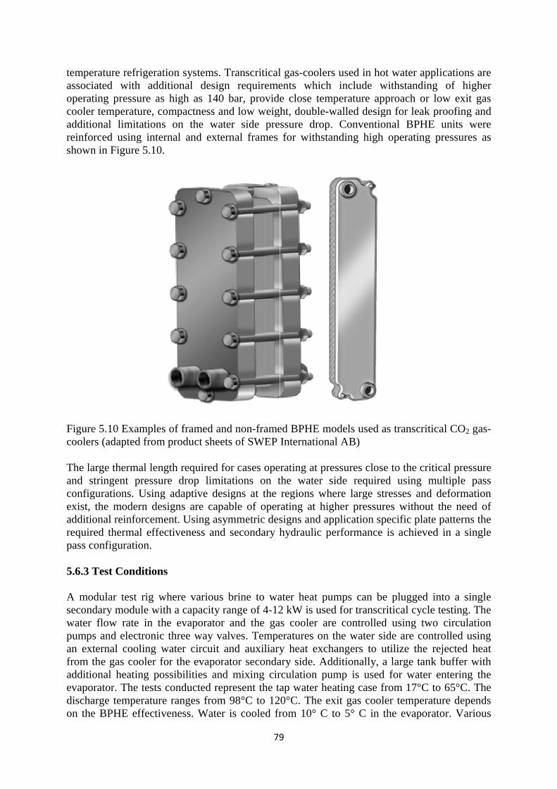
temperature refrigeration systems. Transcritical gasassociated with additional design requirements which incloperating pressure as cooler temperature, compactness and lowadditional limitations on the water side pressurreinforced using internal and external frames for withstashown in Figure 5.1

Figure 5.10 Examples of framed and noncoolers (adapted from product sheets of SWEP International AB) The large thermal length required for cases operating at pressures close to the critical pressure and stringent pressure drop limitations on the water side required using multiple pass configurations. Using adaptive designs at the regions where large stresses and deformation exist, the modern designs are capable of operating at higher pressures without the need of additional reinforcement. Using asymmetric designs and application specific required thermal effectiveness and secondary hydraulic performance is achieved in a single pass configuration. 5.6.3 Test Conditions A modular test rig where various brine to water heat pumps can be plugged into a single secondary moduwater flow rate in pumps and electronic three way valves. Temperatures on the water side are controlled an external cooling water circuit and auxiliary heat exchangers to utilize the rejected heat from the gas cooler foradditional heating possibilities and mixing circulation pump isevaporator. The tests conducted represent the tap water heating case from 17°C to 65°C. The discharge temperature ranges from 98°C to 120°C. The exit gas cooler temperature depends on the BPHE effectiveness. Water is cooled fro

79

temperature refrigeration systems. Transcritical gasassociated with additional design requirements which incloperating pressure as high as 140 bar, provide close temperature approach or low exit gas cooler temperature, compactness and low weight, doubleadditional limitations on the water side pressurreinforced using internal and external frames for withstashown in Figure 5.10.

Examples of framed and non-framed BPHE models used as transcritical CO

coolers (adapted from product sheets of SWEP International AB)

The large thermal length required for cases operating at pressures close to the critical pressure and stringent pressure drop limitations on the water side required using multiple pass

nfigurations. Using adaptive designs at the regions where large stresses and deformation exist, the modern designs are capable of operating at higher pressures without the need of additional reinforcement. Using asymmetric designs and application specific required thermal effectiveness and secondary hydraulic performance is achieved in a single pass configuration.

.3 Test Conditions

A modular test rig where various brine to water heat pumps can be plugged into a single secondary module with a capacity range of 4-12 kW is used for transcritical cycle testing. The water flow rate in the evaporator and the gas cooler are controlled using two circulation pumps and electronic three way valves. Temperatures on the water side are controlled an external cooling water circuit and auxiliary heat exchangers to utilize the rejected heat

gas cooler for the evaporator secondary side. Additionally, a large tank buffer with additional heating possibilities and mixing circulation pump isevaporator. The tests conducted represent the tap water heating case from 17°C to 65°C. The discharge temperature ranges from 98°C to 120°C. The exit gas cooler temperature depends on the BPHE effectiveness. Water is cooled fro

79

temperature refrigeration systems. Transcritical gas-coolers used in hot water applications are associated with additional design requirements which include withstanding of higher

as 140 bar, provide close temperature approach or low exit gas weight, double-walled design for leak proofing and

additional limitations on the water side pressure drop. Conventional BPHE units were reinforced using internal and external frames for withstanding high operating pressures as

framed BPHE models used as transcritical COcoolers (adapted from product sheets of SWEP International AB)

The large thermal length required for cases operating at pressures close to the critical pressure and stringent pressure drop limitations on the water side required using multiple pass

nfigurations. Using adaptive designs at the regions where large stresses and deformation exist, the modern designs are capable of operating at higher pressures without the need of additional reinforcement. Using asymmetric designs and application specific plate patterns the required thermal effectiveness and secondary hydraulic performance is achieved in a single

A modular test rig where various brine to water heat pumps can be plugged into a single 12 kW is used for transcritical cycle testing. The

evaporator and the gas cooler are controlled using two circulation pumps and electronic three way valves. Temperatures on the water side are controlled an external cooling water circuit and auxiliary heat exchangers to utilize the rejected heat

evaporator secondary side. Additionally, a large tank buffer with additional heating possibilities and mixing circulation pump is used for water entering the evaporator. The tests conducted represent the tap water heating case from 17°C to 65°C. The discharge temperature ranges from 98°C to 120°C. The exit gas cooler temperature depends on the BPHE effectiveness. Water is cooled from 10° C to 5° C in the evaporator. Various

coolers used in hot water applications are ude withstanding of higher

as 140 bar, provide close temperature approach or low exit gas walled design for leak proofing and

e drop. Conventional BPHE units were nding high operating pressures as

framed BPHE models used as transcritical CO2 gas-

The large thermal length required for cases operating at pressures close to the critical pressure and stringent pressure drop limitations on the water side required using multiple pass

nfigurations. Using adaptive designs at the regions where large stresses and deformation exist, the modern designs are capable of operating at higher pressures without the need of

plate patterns the required thermal effectiveness and secondary hydraulic performance is achieved in a single

A modular test rig where various brine to water heat pumps can be plugged into a single 12 kW is used for transcritical cycle testing. The

evaporator and the gas cooler are controlled using two circulation pumps and electronic three way valves. Temperatures on the water side are controlled using an external cooling water circuit and auxiliary heat exchangers to utilize the rejected heat

evaporator secondary side. Additionally, a large tank buffer with used for water entering the

evaporator. The tests conducted represent the tap water heating case from 17°C to 65°C. The discharge temperature ranges from 98°C to 120°C. The exit gas cooler temperature depends

m 10° C to 5° C in the evaporator. Various

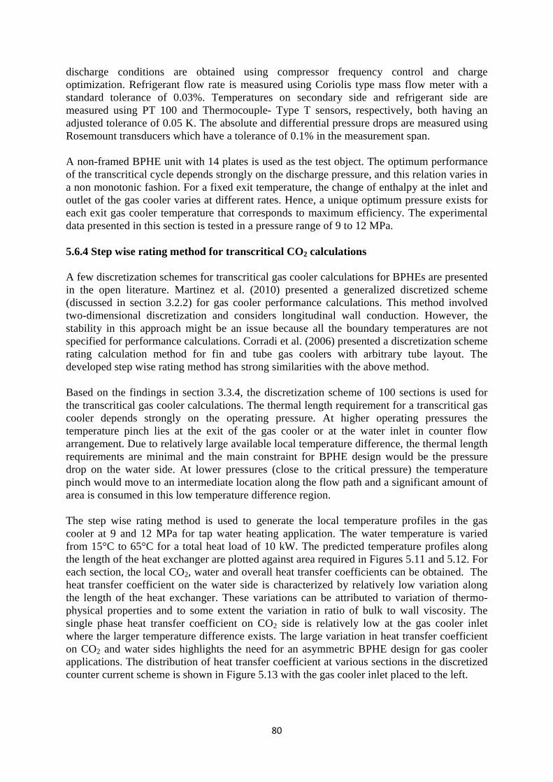
80

discharge conditions are obtained using compressor frequency control and charge optimization. Refrigerant flow rate is measured using Coriolis type mass flow meter with a standard tolerance of 0.03%. Temperatures on secondary side and refrigerant side are measured using PT 100 and Thermocouple- Type T sensors, respectively, both having an adjusted tolerance of 0.05 K. The absolute and differential pressure drops are measured using Rosemount transducers which have a tolerance of 0.1% in the measurement span. A non-framed BPHE unit with 14 plates is used as the test object. The optimum performance of the transcritical cycle depends strongly on the discharge pressure, and this relation varies in a non monotonic fashion. For a fixed exit temperature, the change of enthalpy at the inlet and outlet of the gas cooler varies at different rates. Hence, a unique optimum pressure exists for each exit gas cooler temperature that corresponds to maximum efficiency. The experimental data presented in this section is tested in a pressure range of 9 to 12 MPa. 5.6.4 Step wise rating method for transcritical CO2 calculations A few discretization schemes for transcritical gas cooler calculations for BPHEs are presented in the open literature. Martinez et al. (2010) presented a generalized discretized scheme (discussed in section 3.2.2) for gas cooler performance calculations. This method involved two-dimensional discretization and considers longitudinal wall conduction. However, the stability in this approach might be an issue because all the boundary temperatures are not specified for performance calculations. Corradi et al. (2006) presented a discretization scheme rating calculation method for fin and tube gas coolers with arbitrary tube layout. The developed step wise rating method has strong similarities with the above method. Based on the findings in section 3.3.4, the discretization scheme of 100 sections is used for the transcritical gas cooler calculations. The thermal length requirement for a transcritical gas cooler depends strongly on the operating pressure. At higher operating pressures the temperature pinch lies at the exit of the gas cooler or at the water inlet in counter flow arrangement. Due to relatively large available local temperature difference, the thermal length requirements are minimal and the main constraint for BPHE design would be the pressure drop on the water side. At lower pressures (close to the critical pressure) the temperature pinch would move to an intermediate location along the flow path and a significant amount of area is consumed in this low temperature difference region. The step wise rating method is used to generate the local temperature profiles in the gas cooler at 9 and 12 MPa for tap water heating application. The water temperature is varied from 15°C to 65°C for a total heat load of 10 kW. The predicted temperature profiles along the length of the heat exchanger are plotted against area required in Figures 5.11 and 5.12. For each section, the local CO2, water and overall heat transfer coefficients can be obtained. The heat transfer coefficient on the water side is characterized by relatively low variation along the length of the heat exchanger. These variations can be attributed to variation of thermo-physical properties and to some extent the variation in ratio of bulk to wall viscosity. The single phase heat transfer coefficient on CO2 side is relatively low at the gas cooler inlet where the larger temperature difference exists. The large variation in heat transfer coefficient on CO2 and water sides highlights the need for an asymmetric BPHE design for gas cooler applications. The distribution of heat transfer coefficient at various sections in the discretized counter current scheme is shown in Figure 5.13 with the gas cooler inlet placed to the left.

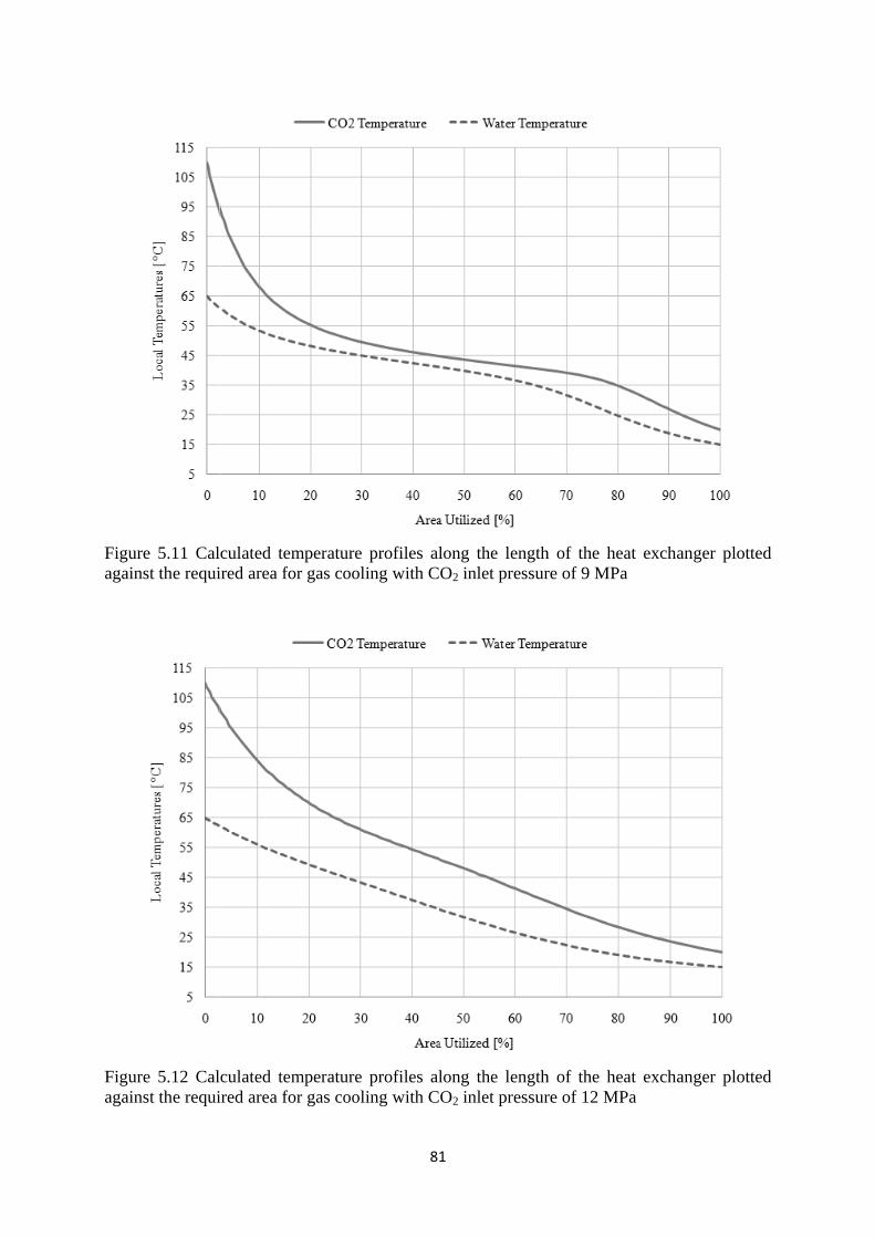
Figure 5.11 Calculated temperature profiles along the length of the heat exchanger plotted against the required

Figure 5.12 Calculated temperature profiles along the length of the heat exchanger plotted against the required

81

Calculated temperature profiles along the length of the heat exchanger plotted against the required area for gas cooling with CO

Calculated temperature profiles along the length of the heat exchanger plotted against the required area for gas cooling with CO

81

Calculated temperature profiles along the length of the heat exchanger plotted for gas cooling with CO2 inlet pressure of 9 MPa

Calculated temperature profiles along the length of the heat exchanger plotted for gas cooling with CO2 inlet pressure of 12 MPa

Calculated temperature profiles along the length of the heat exchanger plotted

Calculated temperature profiles along the length of the heat exchanger plotted

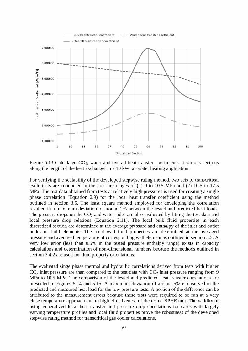
Figure 5.13 Calculated COalong the length of the heat exchanger in a 10 kW tap water heating application For verifying the sccycle tests are conducted in the pressure ranges of (1) 9 to 10.5 MPa and (2) 10.5 MPa. The test data obtained from tests at relatively high pressures is used for creating a single phase correlation (Equation 2.9) for outlined in section 3.5. The least square method employed foresulted in a maximum deviation of around 2% between the tested and predicted heat loads. The pressure drops on the COlocal pressure drop relations (Equation 2.1discretized section are determined at the average pressure and enthalnodes of fluid pressure and averaged tempervery low error (less than 0.5% in calculations and determination of nonsection 3.4.2 are used for fluid property calculations. The evaluated singe phase thermal and hydraulic correlations derived from tests with higher CO2 inlet pressure are than compared to the test data with COMPa to 10.5 MPa. The comparison of the tested and predicted heat transfer correlations are presented in Figures 5.1predicted and measured heat load for the low pressure tests. A porattributed to the measurement errors close temperature approach due to high effectiveness of the tested BPHE unit. The validity of using generalized local heat transfer andvarying temperature profiles and local fluid properties prove the robustness of the developed stepwise rating method for transcritical gas cooler calculations.

82

Calculated CO2, water and overall heat transfer coefficients at various sections the length of the heat exchanger in a 10 kW tap water heating application

For verifying the scalability of the developed stepcycle tests are conducted in the pressure ranges of (1) 9 to 10.5 MPa and (2) 10.5 MPa. The test data obtained from tests at relatively high pressures is used for creating a single phase correlation (Equation 2.9) for the local heat transfer coefficient using the method outlined in section 3.5. The least square method employed foresulted in a maximum deviation of around 2% between the tested and predicted heat loads. The pressure drops on the CO2 and water sides are alslocal pressure drop relations (Equation 2.11). The local bulk fluid properties in each discretized section are determined at the average pressure and enthal

elements. The local wall fluid properties are determined at the averaged pressure and averaged temperature of corresponding wall element as outlined in section 3.3. A very low error (less than 0.5% in the tested pressure enthalpy range) exists in capacity calculations and determination of non-dimensional numbers section 3.4.2 are used for fluid property calculations.

The evaluated singe phase thermal and hydraulic correlations derived from tests with higher inlet pressure are than compared to the test data with CO

MPa to 10.5 MPa. The comparison of the tested and predicted heat transfer correlations are igures 5.14 and 5.15. A maximum deviation of around 5% is observed in the

predicted and measured heat load for the low pressure tests. A porattributed to the measurement errors because close temperature approach due to high effectiveness of the tested BPHE unit. The validity of using generalized local heat transfer and pressure drop correlations for cases with largely varying temperature profiles and local fluid properties prove the robustness of the developed stepwise rating method for transcritical gas cooler calculations.

82

ater and overall heat transfer coefficients at various sections the length of the heat exchanger in a 10 kW tap water heating application

alability of the developed stepwise rating method, two sets of transcritical cycle tests are conducted in the pressure ranges of (1) 9 to 10.5 MPa and (2) 10.5 MPa. The test data obtained from tests at relatively high pressures is used for creating a single

local heat transfer coefficient using the method outlined in section 3.5. The least square method employed for developing the correlation resulted in a maximum deviation of around 2% between the tested and predicted heat loads.

ater sides are also evaluated by fitting the test1). The local bulk fluid properties in each

discretized section are determined at the average pressure and enthalpy of the inlet and outlet elements. The local wall fluid properties are determined at the averaged

ature of corresponding wall element as outlined in section 3.3. A tested pressure enthalpy range) exists in capacity

dimensional numbers because the methods outlined in section 3.4.2 are used for fluid property calculations.

The evaluated singe phase thermal and hydraulic correlations derived from tests with higher inlet pressure are than compared to the test data with CO2 inlet pressure rang

MPa to 10.5 MPa. The comparison of the tested and predicted heat transfer correlations are . A maximum deviation of around 5% is observed in the

predicted and measured heat load for the low pressure tests. A portion of the difference can be these tests were required to be

close temperature approach due to high effectiveness of the tested BPHE unit. The validity of pressure drop correlations for cases with largely

varying temperature profiles and local fluid properties prove the robustness of the developed stepwise rating method for transcritical gas cooler calculations.

ater and overall heat transfer coefficients at various sections

the length of the heat exchanger in a 10 kW tap water heating application

wise rating method, two sets of transcritical cycle tests are conducted in the pressure ranges of (1) 9 to 10.5 MPa and (2) 10.5 to 12.5 MPa. The test data obtained from tests at relatively high pressures is used for creating a single

local heat transfer coefficient using the method r developing the correlation

resulted in a maximum deviation of around 2% between the tested and predicted heat loads. o evaluated by fitting the test data and

1). The local bulk fluid properties in each py of the inlet and outlet

elements. The local wall fluid properties are determined at the averaged ature of corresponding wall element as outlined in section 3.3. A

tested pressure enthalpy range) exists in capacity the methods outlined in

The evaluated singe phase thermal and hydraulic correlations derived from tests with higher inlet pressure ranging from 9

MPa to 10.5 MPa. The comparison of the tested and predicted heat transfer correlations are . A maximum deviation of around 5% is observed in the

tion of the difference can be be run at a very

close temperature approach due to high effectiveness of the tested BPHE unit. The validity of pressure drop correlations for cases with largely

varying temperature profiles and local fluid properties prove the robustness of the developed

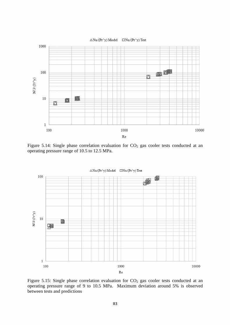
Figure 5.14: Single phase correlation evaluoperating pressure range of 10.5 to 12.5 MPa.

Figure 5.15: Single phase correlation evaluation for COoperating pressure range of 9 to 10.5 MPa. Maximum deviation around 5% is observed between tests and predictions

83

: Single phase correlation evaluation for COoperating pressure range of 10.5 to 12.5 MPa.

: Single phase correlation evaluation for COoperating pressure range of 9 to 10.5 MPa. Maximum deviation around 5% is observed between tests and predictions

83

ation for CO2 gas cooler tests conducted at an

: Single phase correlation evaluation for CO2 gas cooler tests conducted at an operating pressure range of 9 to 10.5 MPa. Maximum deviation around 5% is observed

gas cooler tests conducted at an

gas cooler tests conducted at an

operating pressure range of 9 to 10.5 MPa. Maximum deviation around 5% is observed

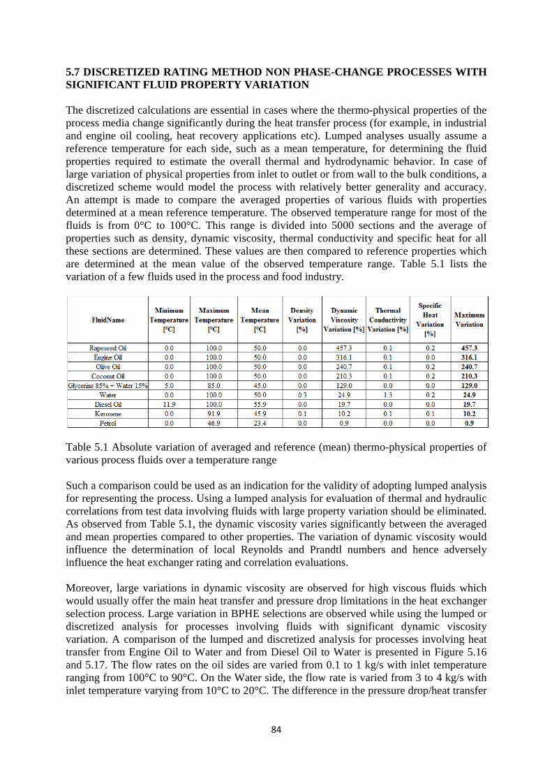
84

5.7 DISCRETIZED RATING METHOD NON PHASE-CHANGE PROCESSES WITH SIGNIFICANT FLUID PROPERTY VARIATION The discretized calculations are essential in cases where the thermo-physical properties of the process media change significantly during the heat transfer process (for example, in industrial and engine oil cooling, heat recovery applications etc). Lumped analyses usually assume a reference temperature for each side, such as a mean temperature, for determining the fluid properties required to estimate the overall thermal and hydrodynamic behavior. In case of large variation of physical properties from inlet to outlet or from wall to the bulk conditions, a discretized scheme would model the process with relatively better generality and accuracy. An attempt is made to compare the averaged properties of various fluids with properties determined at a mean reference temperature. The observed temperature range for most of the fluids is from 0°C to 100°C. This range is divided into 5000 sections and the average of properties such as density, dynamic viscosity, thermal conductivity and specific heat for all these sections are determined. These values are then compared to reference properties which are determined at the mean value of the observed temperature range. Table 5.1 lists the variation of a few fluids used in the process and food industry.

Table 5.1 Absolute variation of averaged and reference (mean) thermo-physical properties of various process fluids over a temperature range Such a comparison could be used as an indication for the validity of adopting lumped analysis for representing the process. Using a lumped analysis for evaluation of thermal and hydraulic correlations from test data involving fluids with large property variation should be eliminated. As observed from Table 5.1, the dynamic viscosity varies significantly between the averaged and mean properties compared to other properties. The variation of dynamic viscosity would influence the determination of local Reynolds and Prandtl numbers and hence adversely influence the heat exchanger rating and correlation evaluations. Moreover, large variations in dynamic viscosity are observed for high viscous fluids which would usually offer the main heat transfer and pressure drop limitations in the heat exchanger selection process. Large variation in BPHE selections are observed while using the lumped or discretized analysis for processes involving fluids with significant dynamic viscosity variation. A comparison of the lumped and discretized analysis for processes involving heat transfer from Engine Oil to Water and from Diesel Oil to Water is presented in Figure 5.16 and 5.17. The flow rates on the oil sides are varied from 0.1 to 1 kg/s with inlet temperature ranging from 100°C to 90°C. On the Water side, the flow rate is varied from 3 to 4 kg/s with inlet temperature varying from 10°C to 20°C. The difference in the pressure drop/heat transfer

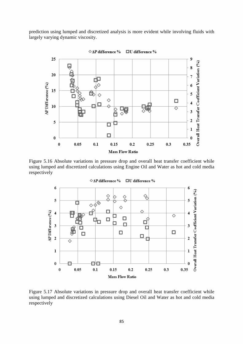
prediction using lumped and discretized analysis is more evident while involving fluids with largely varying dynamic viscosity.

Figure 5.16 Absolute variations in pressure drop and overall heat transfer coefficientusing lumped and discretized calculations using Engine Oil and Water as hot and cold media respectively

Figure 5.17 Absolute variations in pressure drop and overall heat transfer coefficient while using lumped and discretized calculations using Drespectively

85

prediction using lumped and discretized analysis is more evident while involving fluids with largely varying dynamic viscosity.

Absolute variations in pressure drop and overall heat transfer coefficientusing lumped and discretized calculations using Engine Oil and Water as hot and cold media

Absolute variations in pressure drop and overall heat transfer coefficient while using lumped and discretized calculations using D

85

prediction using lumped and discretized analysis is more evident while involving fluids with

Absolute variations in pressure drop and overall heat transfer coefficientusing lumped and discretized calculations using Engine Oil and Water as hot and cold media

Absolute variations in pressure drop and overall heat transfer coefficient while using lumped and discretized calculations using Diesel Oil and Water as hot and cold media

prediction using lumped and discretized analysis is more evident while involving fluids with

Absolute variations in pressure drop and overall heat transfer coefficient while

using lumped and discretized calculations using Engine Oil and Water as hot and cold media

Absolute variations in pressure drop and overall heat transfer coefficient while iesel Oil and Water as hot and cold media

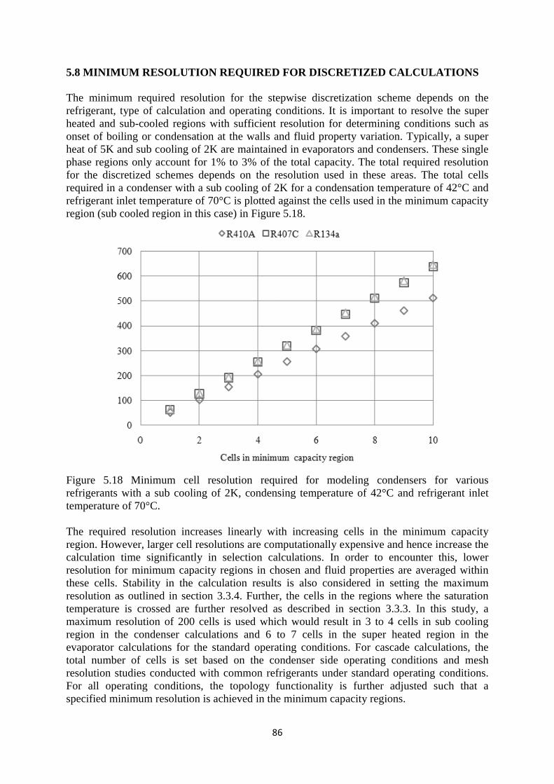
5.8 MINIMUM RESOLUTION REQUIRED FOR DISCRETIZED CALCULATIONS The minimum required resolution for the stepwise discretization scheme depends on the refrigerant, type of calculation and operating condiheated and sub-cooled regions with sufficient resolution for determining conditions such as onset of boiling or condensation at the walls and fluid property variation. Typically, a super heat of 5K and sub coolinphase regions only account for 1% to 3% of the total capacity. The total required resolution for the discretized schemes depends on the resolution used in these areas. The total cells required in a condenser with a sub cooling of 2K for a condensation temperature of 42°C and refrigerant inlet temperature of 70°C is plotted against the cells used in the minimum capacity region (sub cooled region in this case) in

Figure 5.18 Minimum cell resolution required for modeling condensers for various refrigerants with a sub cooling of 2K, condensing temperature of 42°C and refrigerant inlet temperature of 70°C. The required resolution increases linearly with increasing cells in the region. However, larger cell resolutions are computationally expensive and hence increase the calculation time significantly in selection calculations. In order to encounter this, lower resolution for minimum capacity regions in chosen andthese cells. Stability in the calculation results is also considered in setting the maximum resolution as outlined in section 3.3.4. Further, the cells in the regions where the saturation temperature is crossed are furmaximum resolution of 200 cells is used which would result in 3 to 4 cells in sub cooling region in the condenser calculations and 6 to 7 cells in the super heated region in the evaporator calcutotal number of cells is set based on the condenser side operating conditions and mesh resolution studies conducted with common refrigerants under standard operating conditions. For all operating conditions, the topology functionality is further adjusted such that specified minimum resolution is achieved in the minimum capacity regions.

86

MINIMUM RESOLUTION REQUIRED FOR DISCRETIZED CALCULATIONS

The minimum required resolution for the stepwise discretization scheme depends on the refrigerant, type of calculation and operating condi

cooled regions with sufficient resolution for determining conditions such as onset of boiling or condensation at the walls and fluid property variation. Typically, a super heat of 5K and sub cooling of 2K are maintained in evaporators and condensers. These single phase regions only account for 1% to 3% of the total capacity. The total required resolution for the discretized schemes depends on the resolution used in these areas. The total cells

red in a condenser with a sub cooling of 2K for a condensation temperature of 42°C and refrigerant inlet temperature of 70°C is plotted against the cells used in the minimum capacity region (sub cooled region in this case) in Figure 5.

Minimum cell resolution required for modeling condensers for various refrigerants with a sub cooling of 2K, condensing temperature of 42°C and refrigerant inlet temperature of 70°C.

The required resolution increases linearly with increasing cells in the region. However, larger cell resolutions are computationally expensive and hence increase the calculation time significantly in selection calculations. In order to encounter this, lower resolution for minimum capacity regions in chosen andthese cells. Stability in the calculation results is also considered in setting the maximum resolution as outlined in section 3.3.4. Further, the cells in the regions where the saturation temperature is crossed are further resolved as described in section 3.3.3. In this study, a maximum resolution of 200 cells is used which would result in 3 to 4 cells in sub cooling region in the condenser calculations and 6 to 7 cells in the super heated region in the evaporator calculations for the standard operating conditions. For cascade calculations, the total number of cells is set based on the condenser side operating conditions and mesh resolution studies conducted with common refrigerants under standard operating conditions.

or all operating conditions, the topology functionality is further adjusted such that minimum resolution is achieved in the minimum capacity regions.

86

MINIMUM RESOLUTION REQUIRED FOR DISCRETIZED CALCULATIONS

The minimum required resolution for the stepwise discretization scheme depends on the refrigerant, type of calculation and operating conditions. It is important to resolve the super

cooled regions with sufficient resolution for determining conditions such as onset of boiling or condensation at the walls and fluid property variation. Typically, a super

g of 2K are maintained in evaporators and condensers. These single phase regions only account for 1% to 3% of the total capacity. The total required resolution for the discretized schemes depends on the resolution used in these areas. The total cells

red in a condenser with a sub cooling of 2K for a condensation temperature of 42°C and refrigerant inlet temperature of 70°C is plotted against the cells used in the minimum capacity

igure 5.18.

Minimum cell resolution required for modeling condensers for various refrigerants with a sub cooling of 2K, condensing temperature of 42°C and refrigerant inlet

The required resolution increases linearly with increasing cells in the minimum capacity region. However, larger cell resolutions are computationally expensive and hence increase the calculation time significantly in selection calculations. In order to encounter this, lower resolution for minimum capacity regions in chosen and fluid properties are averaged within these cells. Stability in the calculation results is also considered in setting the maximum resolution as outlined in section 3.3.4. Further, the cells in the regions where the saturation

ther resolved as described in section 3.3.3. In this study, a maximum resolution of 200 cells is used which would result in 3 to 4 cells in sub cooling region in the condenser calculations and 6 to 7 cells in the super heated region in the

lations for the standard operating conditions. For cascade calculations, the total number of cells is set based on the condenser side operating conditions and mesh resolution studies conducted with common refrigerants under standard operating conditions.

or all operating conditions, the topology functionality is further adjusted such that minimum resolution is achieved in the minimum capacity regions.

MINIMUM RESOLUTION REQUIRED FOR DISCRETIZED CALCULATIONS

The minimum required resolution for the stepwise discretization scheme depends on the tions. It is important to resolve the super

cooled regions with sufficient resolution for determining conditions such as onset of boiling or condensation at the walls and fluid property variation. Typically, a super

g of 2K are maintained in evaporators and condensers. These single phase regions only account for 1% to 3% of the total capacity. The total required resolution for the discretized schemes depends on the resolution used in these areas. The total cells

red in a condenser with a sub cooling of 2K for a condensation temperature of 42°C and refrigerant inlet temperature of 70°C is plotted against the cells used in the minimum capacity

Minimum cell resolution required for modeling condensers for various

refrigerants with a sub cooling of 2K, condensing temperature of 42°C and refrigerant inlet

minimum capacity region. However, larger cell resolutions are computationally expensive and hence increase the calculation time significantly in selection calculations. In order to encounter this, lower

fluid properties are averaged within these cells. Stability in the calculation results is also considered in setting the maximum resolution as outlined in section 3.3.4. Further, the cells in the regions where the saturation

ther resolved as described in section 3.3.3. In this study, a maximum resolution of 200 cells is used which would result in 3 to 4 cells in sub cooling region in the condenser calculations and 6 to 7 cells in the super heated region in the

lations for the standard operating conditions. For cascade calculations, the total number of cells is set based on the condenser side operating conditions and mesh resolution studies conducted with common refrigerants under standard operating conditions.

or all operating conditions, the topology functionality is further adjusted such that a

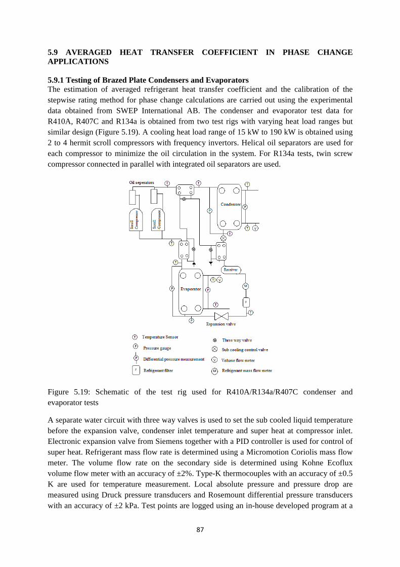
87

5.9 AVERAGED HEAT TRANSFER COEFFICIENT IN PHASE CHANGE APPLICATIONS 5.9.1 Testing of Brazed Plate Condensers and Evaporators The estimation of averaged refrigerant heat transfer coefficient and the calibration of the stepwise rating method for phase change calculations are carried out using the experimental data obtained from SWEP International AB. The condenser and evaporator test data for R410A, R407C and R134a is obtained from two test rigs with varying heat load ranges but similar design (Figure 5.19). A cooling heat load range of 15 kW to 190 kW is obtained using 2 to 4 hermit scroll compressors with frequency invertors. Helical oil separators are used for each compressor to minimize the oil circulation in the system. For R134a tests, twin screw compressor connected in parallel with integrated oil separators are used.

Figure 5.19: Schematic of the test rig used for R410A/R134a/R407C condenser and evaporator tests

A separate water circuit with three way valves is used to set the sub cooled liquid temperature before the expansion valve, condenser inlet temperature and super heat at compressor inlet. Electronic expansion valve from Siemens together with a PID controller is used for control of super heat. Refrigerant mass flow rate is determined using a Micromotion Coriolis mass flow meter. The volume flow rate on the secondary side is determined using Kohne Ecoflux volume flow meter with an accuracy of ±2%. Type-K thermocouples with an accuracy of ±0.5 K are used for temperature measurement. Local absolute pressure and pressure drop are measured using Druck pressure transducers and Rosemount differential pressure transducers with an accuracy of ±2 kPa. Test points are logged using an in-house developed program at a

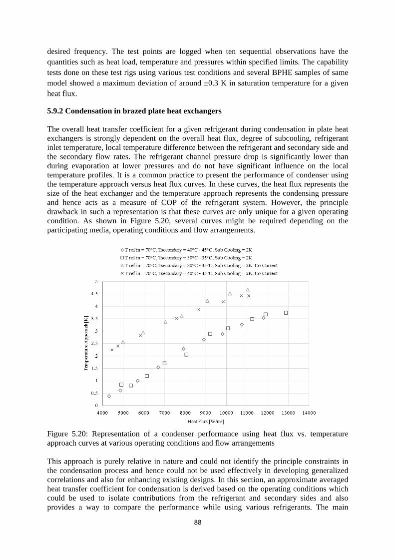
desired frequency. The test points are logged quantities such as heat load, temperature andtests done on these test rigs using various test model showed a maximum deviation of around ±0.3 K in saturation temperature for heat flux.

5.9.2 Condensation in brazed plate heat exchangers The overall heat transfer coefficient for a given refrigerant during condensation in plate heat exchangers is strongly dependent on the overall heat flux, degree of subcooling, refrigerant inlet temperature, local the secondary flow rates. The refrigerant channel pressure drop is significantly lower than during evaporation at lower pressures and do not have significant influence on the local temperature profiles. It is a common practice to present the performance of condenser using the temperature approach versus heat flux curves. In these curves, the heat flux represents the size of the heat exchanger and the temperature approach represents the coand hence acts as a measure of COP of the refrigerant system. However, the principle drawback in such a representation is that these curves are only unique for a given operating condition. As shown in Fparticipating media, operating conditions and flow arrangements.

Figure 5.20: Representation of a condenser performance using heat flux vs. temperature approach curves This approach is purely relative in nature and could not identify the principle constraints in the condensation process and hence could not be used effectively in developing generalized correlations and also for enhancing existing designs. In this heat transfer coefficient for condensation is derived based on the operating conditions which could be used to isolate contributions from the refrigerant and secondary sides and also provides a way to compare the performance while usin

88

desired frequency. The test points are logged quantities such as heat load, temperature and pressures within specified limits. The capability tests done on these test rigs using various test conditionsmodel showed a maximum deviation of around ±0.3 K in saturation temperature for

ation in brazed plate heat exchangers

The overall heat transfer coefficient for a given refrigerant during condensation in plate heat exchangers is strongly dependent on the overall heat flux, degree of subcooling, refrigerant inlet temperature, local temperature difference between the refrigerant and secondary side and the secondary flow rates. The refrigerant channel pressure drop is significantly lower than during evaporation at lower pressures and do not have significant influence on the local

rature profiles. It is a common practice to present the performance of condenser using the temperature approach versus heat flux curves. In these curves, the heat flux represents the size of the heat exchanger and the temperature approach represents the coand hence acts as a measure of COP of the refrigerant system. However, the principle drawback in such a representation is that these curves are only unique for a given operating

. As shown in Figure 5.20, several curves might be participating media, operating conditions and flow arrangements.

: Representation of a condenser performance using heat flux vs. temperature at various operating conditions and flow arrangement

approach is purely relative in nature and could not identify the principle constraints in the condensation process and hence could not be used effectively in developing generalized correlations and also for enhancing existing designs. In this heat transfer coefficient for condensation is derived based on the operating conditions which could be used to isolate contributions from the refrigerant and secondary sides and also

way to compare the performance while usin

88

desired frequency. The test points are logged when ten sequential observations have the pressures within specified limits. The capability conditions and several BPHE samples of same

model showed a maximum deviation of around ±0.3 K in saturation temperature for

ation in brazed plate heat exchangers

The overall heat transfer coefficient for a given refrigerant during condensation in plate heat exchangers is strongly dependent on the overall heat flux, degree of subcooling, refrigerant

temperature difference between the refrigerant and secondary side and the secondary flow rates. The refrigerant channel pressure drop is significantly lower than during evaporation at lower pressures and do not have significant influence on the local

rature profiles. It is a common practice to present the performance of condenser using the temperature approach versus heat flux curves. In these curves, the heat flux represents the size of the heat exchanger and the temperature approach represents the condensing pressure and hence acts as a measure of COP of the refrigerant system. However, the principle drawback in such a representation is that these curves are only unique for a given operating

, several curves might be required depending on the participating media, operating conditions and flow arrangements.

: Representation of a condenser performance using heat flux vs. temperature at various operating conditions and flow arrangements

approach is purely relative in nature and could not identify the principle constraints in the condensation process and hence could not be used effectively in developing generalized correlations and also for enhancing existing designs. In this section, an approximate averagedheat transfer coefficient for condensation is derived based on the operating conditions which could be used to isolate contributions from the refrigerant and secondary sides and also

way to compare the performance while using various refrigerants. The main

sequential observations have the pressures within specified limits. The capability

and several BPHE samples of same model showed a maximum deviation of around ±0.3 K in saturation temperature for a given

The overall heat transfer coefficient for a given refrigerant during condensation in plate heat exchangers is strongly dependent on the overall heat flux, degree of subcooling, refrigerant

temperature difference between the refrigerant and secondary side and the secondary flow rates. The refrigerant channel pressure drop is significantly lower than during evaporation at lower pressures and do not have significant influence on the local

rature profiles. It is a common practice to present the performance of condenser using the temperature approach versus heat flux curves. In these curves, the heat flux represents the

ndensing pressure and hence acts as a measure of COP of the refrigerant system. However, the principle drawback in such a representation is that these curves are only unique for a given operating

required depending on the

: Representation of a condenser performance using heat flux vs. temperature

approach is purely relative in nature and could not identify the principle constraints in the condensation process and hence could not be used effectively in developing generalized

approximate averaged heat transfer coefficient for condensation is derived based on the operating conditions which could be used to isolate contributions from the refrigerant and secondary sides and also

various refrigerants. The main

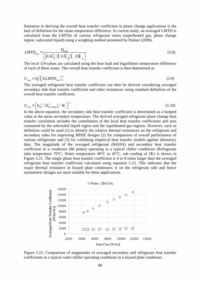
limitation in deriving the overall heat transfer coefficient in phase change applications is the lack of definition for the mean temperature difference. In current study, an averaged LMTD is calculated from the LMTDs of vregion, subcooled liquid) using a weighing method presented by Palmer (2000).

(avgLMTDUA UA UA

=

The local UAvalues are calculated using the heat load and logarithmic temperature difference of each of these zones. The overall heat transfer coefficient is then determined as

( .avg avgU Q A LMTD=The averaged refrigerant heat transfer secondary side heat transfer coefficient and other resistances using standard definition of the overall heat transfer coefficient.

1 1secavg ref ondary rU h h W− − = + +

In the above equation, tvalue at the mean secondary temperature. The derived averaged transfer correlation includesconsumed by the subcooled liquid region and the superheated gas regions. However, such as definition could be used (1)secondary sides for improving BPHE designs (2) various refrigerants and (3) for validating empirical heat transfer models against laboratory data. The magnitude of the averaged refrigerant (R410A) and secondary heat transfer coefficient in a condenser (86 plates) operating in a typinlet temperature 70°C, Water temperature 40°C to 45°C, sub cooling of 2K)Figure 5.21. The single phase heat transfer coefficient is 4 to 8 times larger than the averaged refrigerant heat transfer major thermal resistance in brazed plate condensers is on the refrigerant side and hence asymmetric designs are more suitable for these applications.

Figure 5.21: Comparison of magnitucoefficients in a typical water chiller operating conditions in a

89

limitation in deriving the overall heat transfer coefficient in phase change applications is the lack of definition for the mean temperature difference. In current study, an averaged LMTD is calculated from the LMTDs of various refrigerant zones (super

cooled liquid) using a weighing method presented by Palmer (2000).

) ( ) ( )total

f fg g

Q

UA UA UA + +

values are calculated using the heat load and logarithmic temperature difference of each of these zones. The overall heat transfer coefficient is then determined as

)avg avgU Q A LMTD

The averaged refrigerant heat transfer coefficient can then be derived considering averaged secondary side heat transfer coefficient and other resistances using standard definition of the overall heat transfer coefficient.

11 1secavg ref ondary rU h h W

−− − = + +

In the above equation, the secondary side heat transfer coefficient is determined as a lumped value at the mean secondary temperature. The derived averaged transfer correlation includes the contribution of the local heat transfer coefficients and areconsumed by the subcooled liquid region and the superheated gas regions. However, such as definition could be used (1) to identify the relative thermal resistances on the refrigerant and secondary sides for improving BPHE designs (2) various refrigerants and (3) for validating empirical heat transfer models against laboratory data. The magnitude of the averaged refrigerant (R410A) and secondary heat transfer coefficient in a condenser (86 plates) operating in a typinlet temperature 70°C, Water temperature 40°C to 45°C, sub cooling of 2K)

. The single phase heat transfer coefficient is 4 to 8 times larger than the averaged refrigerant heat transfer coefficient calculated using equation 5.1major thermal resistance in brazed plate condensers is on the refrigerant side and hence asymmetric designs are more suitable for these applications.

: Comparison of magnitudes of averaged secondary and refrigerant heat transfer coefficients in a typical water chiller operating conditions in a

89

limitation in deriving the overall heat transfer coefficient in phase change applications is the lack of definition for the mean temperature difference. In current study, an averaged LMTD is

ious refrigerant zones (superheated gas, phase change cooled liquid) using a weighing method presented by Palmer (2000).

values are calculated using the heat load and logarithmic temperature difference of each of these zones. The overall heat transfer coefficient is then determined as

coefficient can then be derived considering averaged secondary side heat transfer coefficient and other resistances using standard definition of the

he secondary side heat transfer coefficient is determined as a lumped value at the mean secondary temperature. The derived averaged refrigerant phase change heat

the contribution of the local heat transfer coefficients and areconsumed by the subcooled liquid region and the superheated gas regions. However, such as

identify the relative thermal resistances on the refrigerant and secondary sides for improving BPHE designs (2) for comparison of overall performance of various refrigerants and (3) for validating empirical heat transfer models against laboratory data. The magnitude of the averaged refrigerant (R410A) and secondary heat transfer coefficient in a condenser (86 plates) operating in a typical chiller conditions (Refrigerant inlet temperature 70°C, Water temperature 40°C to 45°C, sub cooling of 2K)

. The single phase heat transfer coefficient is 4 to 8 times larger than the averaged coefficient calculated using equation 5.12. This indicate

major thermal resistance in brazed plate condensers is on the refrigerant side and hence asymmetric designs are more suitable for these applications.

des of averaged secondary and refrigerant heat transfer coefficients in a typical water chiller operating conditions in a brazed plate condenser.

limitation in deriving the overall heat transfer coefficient in phase change applications is the lack of definition for the mean temperature difference. In current study, an averaged LMTD is

d gas, phase change cooled liquid) using a weighing method presented by Palmer (2000).

(5.8)

values are calculated using the heat load and logarithmic temperature difference of each of these zones. The overall heat transfer coefficient is then determined as

(5.9)

coefficient can then be derived considering averaged secondary side heat transfer coefficient and other resistances using standard definition of the

(5.10)

he secondary side heat transfer coefficient is determined as a lumped refrigerant phase change heat

the contribution of the local heat transfer coefficients and area consumed by the subcooled liquid region and the superheated gas regions. However, such as

identify the relative thermal resistances on the refrigerant and erall performance of

various refrigerants and (3) for validating empirical heat transfer models against laboratory data. The magnitude of the averaged refrigerant (R410A) and secondary heat transfer

ical chiller conditions (Refrigerant inlet temperature 70°C, Water temperature 40°C to 45°C, sub cooling of 2K) is shown in

. The single phase heat transfer coefficient is 4 to 8 times larger than the averaged . This indicates that the

major thermal resistance in brazed plate condensers is on the refrigerant side and hence

- des of averaged secondary and refrigerant heat transfer

condenser.

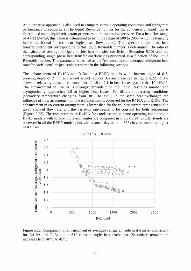
An alternative approach is also used to compare various operating conditions and refrigerant performance in codetermined using liquid refrigerant properties at the saturation pressure. For a heat flux range of 4 - 12 kW/m², this value is determined to be in the range of 500 to 2000 (which is tyin the transitionaltransfer coefficient corresponding to this liquid Reynolds number is determined. The ratio of the calculated average refrigerant side heat transfer coefficcorresponding single phase heat transfer coefficient is presented as a function of the liquid Reynolds number. This parameter is termed as the “enhancement of averaged refrigerant heat transfer coefficient” or just “enhancement The enhancement of R410A and R134a in a BPHE models with chevron angle of 61°, pressing depth of 2 mm and a cell aspect ratio of shows a relatively constant enhancement of 1.9 to 2.1 in The enhancement in R410A is strongly dependent on the liquid Reynolds number and asymptotically approaches 1.5 at higher heat fluxes. For different operating conditions (secondary temperature changing from 30°C to 35°C) ininfluence of flow arrangement on the enhancement is observed for the R410A and R134a. The enhancement in cogiven channel flow rate, and the variation (Figure 5.23). The enhancement in R410A for condensation at same operating conditions in BPHE models with different chevron angles are compared in observed in all the BPHE modeheat fluxes.

Figure 5.22: Comparison of enhancement of averaged refrigerant side heat transfer coefficient for R410A and R134a in a 61° chevron angle heat exchanger (Secondary temperature increases from 40°C to 45°C)

90

An alternative approach is also used to compare various operating conditions and refrigerant performance in condensers. The liquid Reynolds number for the condenser channel flow is determined using liquid refrigerant properties at the saturation pressure. For a heat flux range

12 kW/m², this value is determined to be in the range of 500 to 2000 (which is tyin the transitional-full turbulent single phase flow region). The expected single phase heat transfer coefficient corresponding to this liquid Reynolds number is determined. The ratio of the calculated average refrigerant side heat transfer coefficcorresponding single phase heat transfer coefficient is presented as a function of the liquid Reynolds number. This parameter is termed as the “enhancement of averaged refrigerant heat transfer coefficient” or just “enhancement” in the following sections.

The enhancement of R410A and R134a in a BPHE models with chevron angle of 61°, pressing depth of 2 mm and a cell aspect ratio of shows a relatively constant enhancement of 1.9 to 2.1 in The enhancement in R410A is strongly dependent on the liquid Reynolds number and asymptotically approaches 1.5 at higher heat fluxes. For different operating conditions (secondary temperature changing from 30°C to 35°C) ininfluence of flow arrangement on the enhancement is observed for the R410A and R134a. The enhancement in co-current arrangement is lower than for the counter current arrangement at a given channel flow rate, and the variation rate seems to be constant for both refrigerants

). The enhancement in R410A for condensation at same operating conditions in BPHE models with different chevron angles are compared in observed in all the BPHE models, but with a small deviation in 58° chevron model at higher

: Comparison of enhancement of averaged refrigerant side heat transfer coefficient for R410A and R134a in a 61° chevron angle heat exchanger (Secondary temperature

reases from 40°C to 45°C)

90

An alternative approach is also used to compare various operating conditions and refrigerant ndensers. The liquid Reynolds number for the condenser channel flow is

determined using liquid refrigerant properties at the saturation pressure. For a heat flux range 12 kW/m², this value is determined to be in the range of 500 to 2000 (which is ty

full turbulent single phase flow region). The expected single phase heat transfer coefficient corresponding to this liquid Reynolds number is determined. The ratio of the calculated average refrigerant side heat transfer coefficient (Equation 5.1corresponding single phase heat transfer coefficient is presented as a function of the liquid Reynolds number. This parameter is termed as the “enhancement of averaged refrigerant heat

” in the following sections.

The enhancement of R410A and R134a in a BPHE models with chevron angle of 61°, pressing depth of 2 mm and a cell aspect ratio of 3.5 are presented in figure 5.2shows a relatively constant enhancement of 1.9 to 2.1 in heat fluxes greater than10 kW/m². The enhancement in R410A is strongly dependent on the liquid Reynolds number and asymptotically approaches 1.5 at higher heat fluxes. For different operating conditions (secondary temperature changing from 30°C to 35°C) in the same heat exchanger, the influence of flow arrangement on the enhancement is observed for the R410A and R134a. The

current arrangement is lower than for the counter current arrangement at a rate seems to be constant for both refrigerants

). The enhancement in R410A for condensation at same operating conditions in BPHE models with different chevron angles are compared in Figure 5.24. Similar trends are

small deviation in 58° chevron model at higher

: Comparison of enhancement of averaged refrigerant side heat transfer coefficient for R410A and R134a in a 61° chevron angle heat exchanger (Secondary temperature

An alternative approach is also used to compare various operating conditions and refrigerant ndensers. The liquid Reynolds number for the condenser channel flow is

determined using liquid refrigerant properties at the saturation pressure. For a heat flux range 12 kW/m², this value is determined to be in the range of 500 to 2000 (which is typically

full turbulent single phase flow region). The expected single phase heat transfer coefficient corresponding to this liquid Reynolds number is determined. The ratio of

ient (Equation 5.10) and the corresponding single phase heat transfer coefficient is presented as a function of the liquid Reynolds number. This parameter is termed as the “enhancement of averaged refrigerant heat

The enhancement of R410A and R134a in a BPHE models with chevron angle of 61°, 3.5 are presented in figure 5.22. R134a

heat fluxes greater than10 kW/m². The enhancement in R410A is strongly dependent on the liquid Reynolds number and asymptotically approaches 1.5 at higher heat fluxes. For different operating conditions

the same heat exchanger, the influence of flow arrangement on the enhancement is observed for the R410A and R134a. The

current arrangement is lower than for the counter current arrangement at a rate seems to be constant for both refrigerants

). The enhancement in R410A for condensation at same operating conditions in . Similar trends are

small deviation in 58° chevron model at higher

: Comparison of enhancement of averaged refrigerant side heat transfer coefficient for R410A and R134a in a 61° chevron angle heat exchanger (Secondary temperature

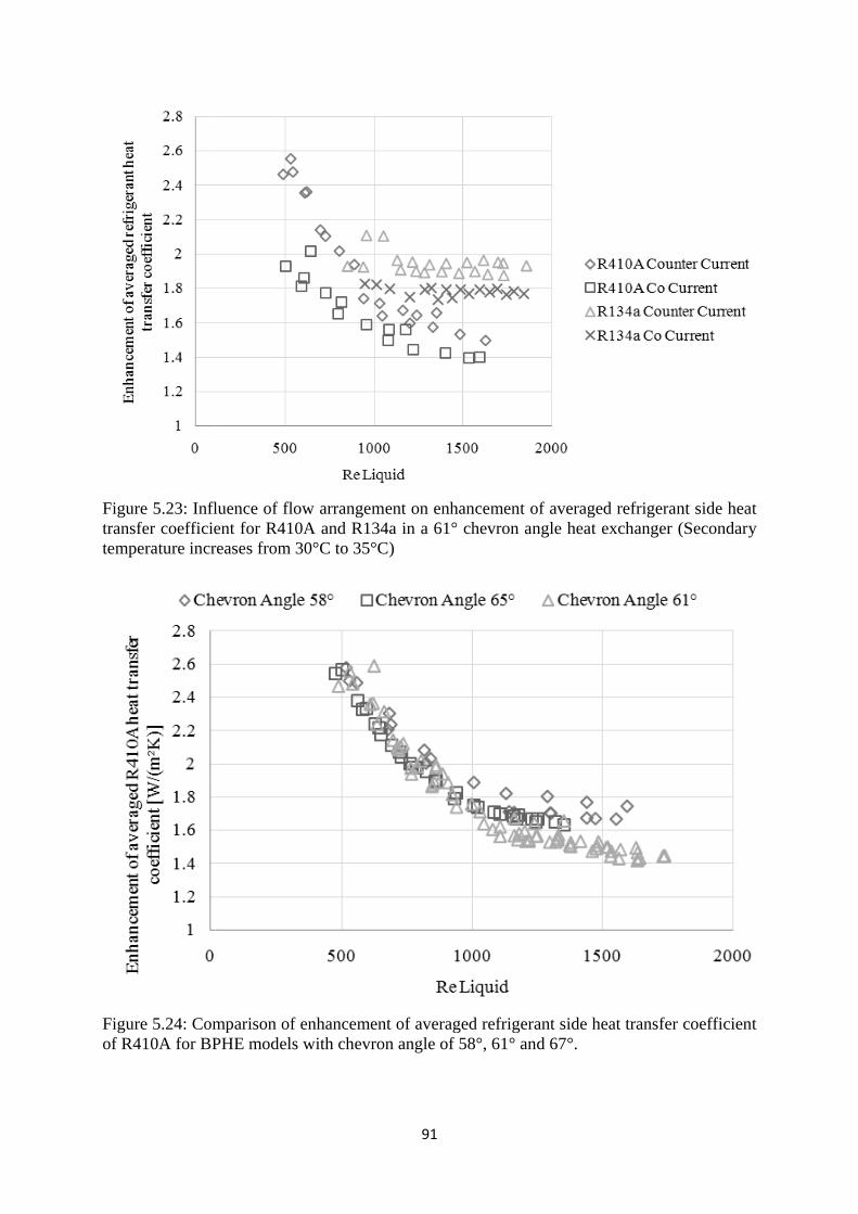
Figure 5.23: Influence of flow arrangement on enhancement of averaged refrigerant side heat transfer coefficient for R410A and R134a in a 61° chevron angle heat exchanger (Secondary temperature increases from 30°C to 35°C)

Figure 5.24: Comparison of enhancement of averaged refrigerant side heat transfer coefficient of R410A for BPHE models with chevron angle of 58°, 61° and 67°.

91

: Influence of flow arrangement on enhancement of averaged refrigerant side heat transfer coefficient for R410A and R134a in a 61° chevron angle heat exchanger (Secondary temperature increases from 30°C to 35°C)

: Comparison of enhancement of averaged refrigerant side heat transfer coefficient of R410A for BPHE models with chevron angle of 58°, 61° and 67°.

91

: Influence of flow arrangement on enhancement of averaged refrigerant side heat transfer coefficient for R410A and R134a in a 61° chevron angle heat exchanger (Secondary

: Comparison of enhancement of averaged refrigerant side heat transfer coefficient of R410A for BPHE models with chevron angle of 58°, 61° and 67°.

: Influence of flow arrangement on enhancement of averaged refrigerant side heat

transfer coefficient for R410A and R134a in a 61° chevron angle heat exchanger (Secondary

: Comparison of enhancement of averaged refrigerant side heat transfer coefficient

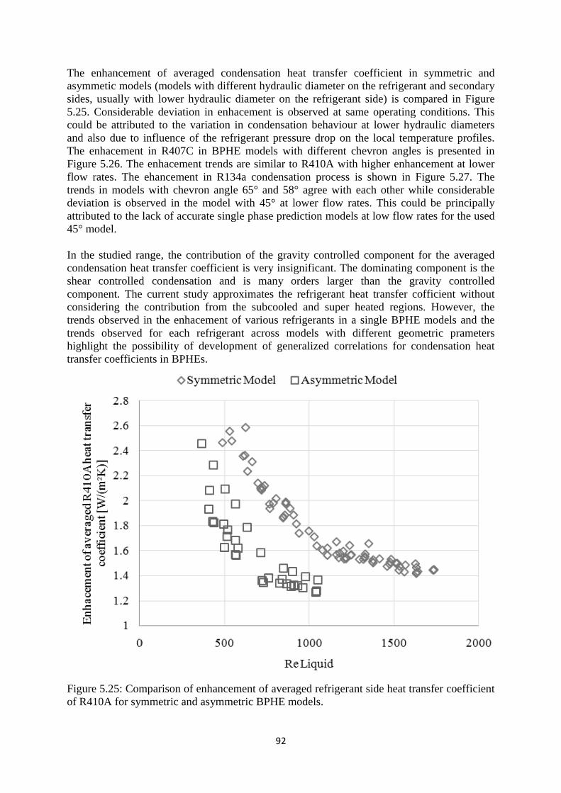
The enhancement of averaged condensation heat transfer coefficient in symmetrasymmetic models (models with different hydraulic diameter on the refrigerant and secondary sides, usually with lower hydraulic diameter on the refrigerant side) is compared in 5.25. Considerable deviation in enhacement is observed at scould be attributed to the variation in condensation behaviour at lower hydraulic diameters and also due to influence of the refrigerant pressure drop on the local temperature profiles. The enhacement in R407C in BPHE models with diFigure 5.26. The enhacement trends are similar to R410A with higher enhancement at lower flow rates. The ehancement in R134a condensation process is shown in trends in models with chevron angle 65° andeviation is observed in the model with 45° at lower flow rates. This could be principally attributed to the lack of accurate single phase prediction models at low flow rates for the used 45° model. In the studied range, the contribution of the gravity controlled component for the averaged condensation heat transfer coefficient is very insignificant. The dominating componeshear controlled condensation and is many orders larger than the gravity controcomponent. The current study approximates the refrigerant heat transfer cofficient without considering the contribution from the subcooled and super heated regions. However, the trends observed in the enhacement of various refrigerants in a single BPHtrends observed for each refrigerant across models with different geometric prameters highlight the possibility of development of generalized correlations for condensation heat transfer coefficients in BPHEs.

Figure 5.25: Comparison of enhancement of averaged refrigerant side heat transfer coefficient of R410A for symmetric and asymmetric BPHE models.

92

The enhancement of averaged condensation heat transfer coefficient in symmetrasymmetic models (models with different hydraulic diameter on the refrigerant and secondary sides, usually with lower hydraulic diameter on the refrigerant side) is compared in

. Considerable deviation in enhacement is observed at scould be attributed to the variation in condensation behaviour at lower hydraulic diameters and also due to influence of the refrigerant pressure drop on the local temperature profiles. The enhacement in R407C in BPHE models with di

. The enhacement trends are similar to R410A with higher enhancement at lower flow rates. The ehancement in R134a condensation process is shown in trends in models with chevron angle 65° and 58° agree with each other while considerable deviation is observed in the model with 45° at lower flow rates. This could be principally attributed to the lack of accurate single phase prediction models at low flow rates for the used

range, the contribution of the gravity controlled component for the averaged condensation heat transfer coefficient is very insignificant. The dominating componeshear controlled condensation and is many orders larger than the gravity controcomponent. The current study approximates the refrigerant heat transfer cofficient without considering the contribution from the subcooled and super heated regions. However, the trends observed in the enhacement of various refrigerants in a single BPHtrends observed for each refrigerant across models with different geometric prameters highlight the possibility of development of generalized correlations for condensation heat transfer coefficients in BPHEs.

: Comparison of enhancement of averaged refrigerant side heat transfer coefficient of R410A for symmetric and asymmetric BPHE models.

92

The enhancement of averaged condensation heat transfer coefficient in symmetrasymmetic models (models with different hydraulic diameter on the refrigerant and secondary sides, usually with lower hydraulic diameter on the refrigerant side) is compared in

. Considerable deviation in enhacement is observed at same operating conditions. This could be attributed to the variation in condensation behaviour at lower hydraulic diameters and also due to influence of the refrigerant pressure drop on the local temperature profiles. The enhacement in R407C in BPHE models with different chevron angles is presented in

. The enhacement trends are similar to R410A with higher enhancement at lower flow rates. The ehancement in R134a condensation process is shown in Figure 5.2

d 58° agree with each other while considerable deviation is observed in the model with 45° at lower flow rates. This could be principally attributed to the lack of accurate single phase prediction models at low flow rates for the used

range, the contribution of the gravity controlled component for the averaged condensation heat transfer coefficient is very insignificant. The dominating componeshear controlled condensation and is many orders larger than the gravity controcomponent. The current study approximates the refrigerant heat transfer cofficient without considering the contribution from the subcooled and super heated regions. However, the trends observed in the enhacement of various refrigerants in a single BPHE models and the trends observed for each refrigerant across models with different geometric prameters highlight the possibility of development of generalized correlations for condensation heat

: Comparison of enhancement of averaged refrigerant side heat transfer coefficient of R410A for symmetric and asymmetric BPHE models.

The enhancement of averaged condensation heat transfer coefficient in symmetric and asymmetic models (models with different hydraulic diameter on the refrigerant and secondary sides, usually with lower hydraulic diameter on the refrigerant side) is compared in Figure

rating conditions. This could be attributed to the variation in condensation behaviour at lower hydraulic diameters and also due to influence of the refrigerant pressure drop on the local temperature profiles.

gles is presented in . The enhacement trends are similar to R410A with higher enhancement at lower

igure 5.27. The d 58° agree with each other while considerable

deviation is observed in the model with 45° at lower flow rates. This could be principally attributed to the lack of accurate single phase prediction models at low flow rates for the used

range, the contribution of the gravity controlled component for the averaged condensation heat transfer coefficient is very insignificant. The dominating component is the shear controlled condensation and is many orders larger than the gravity controlled component. The current study approximates the refrigerant heat transfer cofficient without considering the contribution from the subcooled and super heated regions. However, the

E models and the trends observed for each refrigerant across models with different geometric prameters highlight the possibility of development of generalized correlations for condensation heat

: Comparison of enhancement of averaged refrigerant side heat transfer coefficient

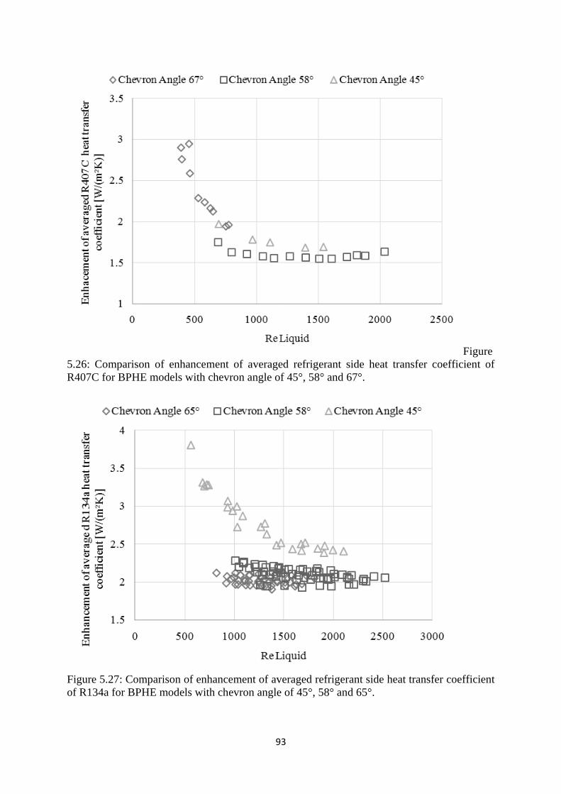
5.26: Comparison of enhancement of averaged refrigerant side heat transfer coefficient of R407C for BPHE models

Figure 5.27: Comparison of enhancement of averaged refrigerant side heat transfer coefficient of R134a for BPHE models with chevron angle of 45°, 58° and 65°.

93

: Comparison of enhancement of averaged refrigerant side heat transfer coefficient of R407C for BPHE models with chevron angle of 45°, 58° and 67°.

: Comparison of enhancement of averaged refrigerant side heat transfer coefficient of R134a for BPHE models with chevron angle of 45°, 58° and 65°.

93

: Comparison of enhancement of averaged refrigerant side heat transfer coefficient of with chevron angle of 45°, 58° and 67°.

: Comparison of enhancement of averaged refrigerant side heat transfer coefficient of R134a for BPHE models with chevron angle of 45°, 58° and 65°.

Figure : Comparison of enhancement of averaged refrigerant side heat transfer coefficient of

: Comparison of enhancement of averaged refrigerant side heat transfer coefficient

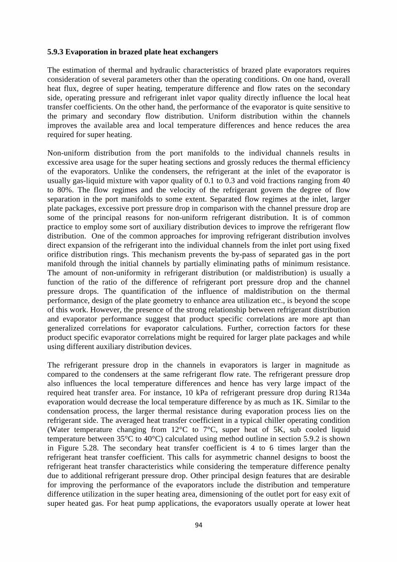
94

5.9.3 Evaporation in brazed plate heat exchangers The estimation of thermal and hydraulic characteristics of brazed plate evaporators requires consideration of several parameters other than the operating conditions. On one hand, overall heat flux, degree of super heating, temperature difference and flow rates on the secondary side, operating pressure and refrigerant inlet vapor quality directly influence the local heat transfer coefficients. On the other hand, the performance of the evaporator is quite sensitive to the primary and secondary flow distribution. Uniform distribution within the channels improves the available area and local temperature differences and hence reduces the area required for super heating. Non-uniform distribution from the port manifolds to the individual channels results in excessive area usage for the super heating sections and grossly reduces the thermal efficiency of the evaporators. Unlike the condensers, the refrigerant at the inlet of the evaporator is usually gas-liquid mixture with vapor quality of 0.1 to 0.3 and void fractions ranging from 40 to 80%. The flow regimes and the velocity of the refrigerant govern the degree of flow separation in the port manifolds to some extent. Separated flow regimes at the inlet, larger plate packages, excessive port pressure drop in comparison with the channel pressure drop are some of the principal reasons for non-uniform refrigerant distribution. It is of common practice to employ some sort of auxiliary distribution devices to improve the refrigerant flow distribution. One of the common approaches for improving refrigerant distribution involves direct expansion of the refrigerant into the individual channels from the inlet port using fixed orifice distribution rings. This mechanism prevents the by-pass of separated gas in the port manifold through the initial channels by partially eliminating paths of minimum resistance. The amount of non-uniformity in refrigerant distribution (or maldistribution) is usually a function of the ratio of the difference of refrigerant port pressure drop and the channel pressure drops. The quantification of the influence of maldistribution on the thermal performance, design of the plate geometry to enhance area utilization etc., is beyond the scope of this work. However, the presence of the strong relationship between refrigerant distribution and evaporator performance suggest that product specific correlations are more apt than generalized correlations for evaporator calculations. Further, correction factors for these product specific evaporator correlations might be required for larger plate packages and while using different auxiliary distribution devices. The refrigerant pressure drop in the channels in evaporators is larger in magnitude as compared to the condensers at the same refrigerant flow rate. The refrigerant pressure drop also influences the local temperature differences and hence has very large impact of the required heat transfer area. For instance, 10 kPa of refrigerant pressure drop during R134a evaporation would decrease the local temperature difference by as much as 1K. Similar to the condensation process, the larger thermal resistance during evaporation process lies on the refrigerant side. The averaged heat transfer coefficient in a typical chiller operating condition (Water temperature changing from 12°C to 7°C, super heat of 5K, sub cooled liquid temperature between 35°C to 40°C) calculated using method outline in section 5.9.2 is shown in Figure 5.28. The secondary heat transfer coefficient is 4 to 6 times larger than the refrigerant heat transfer coefficient. This calls for asymmetric channel designs to boost the refrigerant heat transfer characteristics while considering the temperature difference penalty due to additional refrigerant pressure drop. Other principal design features that are desirable for improving the performance of the evaporators include the distribution and temperature difference utilization in the super heating area, dimensioning of the outlet port for easy exit of super heated gas. For heat pump applications, the evaporators usually operate at lower heat

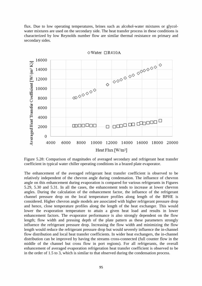
flux. Due to low operating temperatures, brines such as alcoholwater mixtures are used on the secondarcharacterized by low Reynolds number flow are similar thermal resistance on primary and secondary sides.

Figure 5.28: Comparison of magnitudes of averaged secondary and refrigerant heat transfer coefficient in typical water chiller operating conditions in a The enhancement of the averaged refrigerant heat transfer coefficient is observed to be relatively independent of the chevron angle during condensation. The influence angle on this enhancement during evaporation is compared for various refrigerants in Figures 5.29, 5.30 and 5.3angles. During the calculation of the enhancement factor, the channel pressure drop on the local temperature profiles along length of the BPHE is considered. Higher chevron angle models are associated with higher refrigerant pressure drop and hence, close temperature profiles along the lelower the evaporation temperature to attain a given heat load and results in lower enhancement factors. The evaporator performance is also strongly dependent on the flow length; flow width and pressing depth of the plinfluence the refrigerant pressure drop. Increasing the flow width and minimizing the flow length would reduce the refrigerant pressure drop but would severely influence the inflow distribution and local hedistribution can be improved by having the streammiddle of the channel but cross flow in port regions). For all refrigerants, the overall enhancement of averaged evaporation refrigeration heat transfer coefficient is observed to be in the order of 1.5 to 3, which is similar to that observed during the condensation process.

95

flux. Due to low operating temperatures, brines such as alcoholwater mixtures are used on the secondary side. The heat transfer process in these conditions is characterized by low Reynolds number flow are similar thermal resistance on primary and secondary sides.

: Comparison of magnitudes of averaged secondary and refrigerant heat transfer coefficient in typical water chiller operating conditions in a

The enhancement of the averaged refrigerant heat transfer coefficient is observed to be relatively independent of the chevron angle during condensation. The influence angle on this enhancement during evaporation is compared for various refrigerants in Figures

and 5.31. In all the cases, the enhancement tends to increase at lower chevron angles. During the calculation of the enhancement factor, the channel pressure drop on the local temperature profiles along length of the BPHE is considered. Higher chevron angle models are associated with higher refrigerant pressure drop and hence, close temperature profiles along the lelower the evaporation temperature to attain a given heat load and results in lower enhancement factors. The evaporator performance is also strongly dependent on the flow length; flow width and pressing depth of the plinfluence the refrigerant pressure drop. Increasing the flow width and minimizing the flow length would reduce the refrigerant pressure drop but would severely influence the inflow distribution and local heat transfer coefficients. In wider heat exchangers, the indistribution can be improved by having the streammiddle of the channel but cross flow in port regions). For all refrigerants, the overall

ment of averaged evaporation refrigeration heat transfer coefficient is observed to be in the order of 1.5 to 3, which is similar to that observed during the condensation process.

95

flux. Due to low operating temperatures, brines such as alcohol-water mixtures or glycoly side. The heat transfer process in these conditions is

characterized by low Reynolds number flow are similar thermal resistance on primary and

: Comparison of magnitudes of averaged secondary and refrigerant heat transfer coefficient in typical water chiller operating conditions in a brazed plate evaporator.

The enhancement of the averaged refrigerant heat transfer coefficient is observed to be relatively independent of the chevron angle during condensation. The influence angle on this enhancement during evaporation is compared for various refrigerants in Figures

. In all the cases, the enhancement tends to increase at lower chevron angles. During the calculation of the enhancement factor, the influence of the refrigerant channel pressure drop on the local temperature profiles along length of the BPHE is considered. Higher chevron angle models are associated with higher refrigerant pressure drop and hence, close temperature profiles along the length of the heat exchanger. This would lower the evaporation temperature to attain a given heat load and results in lower enhancement factors. The evaporator performance is also strongly dependent on the flow length; flow width and pressing depth of the plate pattern as these parameters strongly influence the refrigerant pressure drop. Increasing the flow width and minimizing the flow length would reduce the refrigerant pressure drop but would severely influence the in

at transfer coefficients. In wider heat exchangers, the indistribution can be improved by having the streams cross-connected (full counter flow in the middle of the channel but cross flow in port regions). For all refrigerants, the overall

ment of averaged evaporation refrigeration heat transfer coefficient is observed to be in the order of 1.5 to 3, which is similar to that observed during the condensation process.

water mixtures or glycol-y side. The heat transfer process in these conditions is

characterized by low Reynolds number flow are similar thermal resistance on primary and

: Comparison of magnitudes of averaged secondary and refrigerant heat transfer

evaporator.

The enhancement of the averaged refrigerant heat transfer coefficient is observed to be relatively independent of the chevron angle during condensation. The influence of chevron angle on this enhancement during evaporation is compared for various refrigerants in Figures

. In all the cases, the enhancement tends to increase at lower chevron influence of the refrigerant

channel pressure drop on the local temperature profiles along length of the BPHE is considered. Higher chevron angle models are associated with higher refrigerant pressure drop

ngth of the heat exchanger. This would lower the evaporation temperature to attain a given heat load and results in lower enhancement factors. The evaporator performance is also strongly dependent on the flow

ate pattern as these parameters strongly influence the refrigerant pressure drop. Increasing the flow width and minimizing the flow length would reduce the refrigerant pressure drop but would severely influence the in-channel

at transfer coefficients. In wider heat exchangers, the in-channel connected (full counter flow in the

middle of the channel but cross flow in port regions). For all refrigerants, the overall ment of averaged evaporation refrigeration heat transfer coefficient is observed to be

in the order of 1.5 to 3, which is similar to that observed during the condensation process.

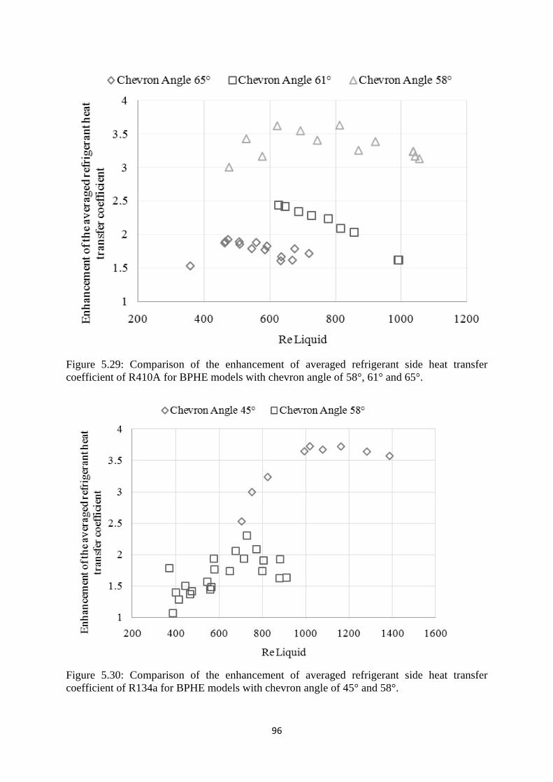
Figure 5.29: Comparison of the enhancement of averaged refrigerant side hcoefficient of R410A for BPHE models with chevron angle of 58°, 61° and 65°.

Figure 5.30: Comparison of the enhancement of averaged refrigerant side heat transfer coefficient of R134a for BPHE models with chevron angle of 45° and 58°.

96

: Comparison of the enhancement of averaged refrigerant side hcoefficient of R410A for BPHE models with chevron angle of 58°, 61° and 65°.

: Comparison of the enhancement of averaged refrigerant side heat transfer coefficient of R134a for BPHE models with chevron angle of 45° and 58°.

96

: Comparison of the enhancement of averaged refrigerant side hcoefficient of R410A for BPHE models with chevron angle of 58°, 61° and 65°.

: Comparison of the enhancement of averaged refrigerant side heat transfer coefficient of R134a for BPHE models with chevron angle of 45° and 58°.

: Comparison of the enhancement of averaged refrigerant side heat transfer

coefficient of R410A for BPHE models with chevron angle of 58°, 61° and 65°.

: Comparison of the enhancement of averaged refrigerant side heat transfer

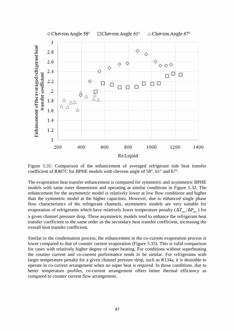
Figure 5.31: Comparison of the enhancement of averaged refrigerant side heat transfer coefficient of R407C for BPHE models with chevron angle of 58°, 61° and 67°. The evaporation heat transfer enhancement is compared for symmetric and asymmetric BPHE models with same outer dimensions and operating at similar conditions in Figure 5.3enhancement for the asymmetric model is relatively lower at low flow conditions and higher than the symmetric model at the higher capacities. However, due to enhancedflow characteristics of the refrigerant channels, asymmetric models are very suitable for evaporation of refrigerants

a given channel pressure drop. These asymmetric models tend to enhance the refrigerant heat transfer coefficient to the same order as the secondary heat transfer coefficient, increasing the overall heat transfer coefficient. Similar to the condensalower compared to that of counter current evaporation (Figure 5.3for cases with relatively higher degree of super heating. For conditions without superheatithe counter current and colarger temperature penalty for a given channel pressure drop, such as R134a, it is desirable to operate in co-current arrangement better temperature profiles, cocompared to counter current flow arrangement.

97

: Comparison of the enhancement of averaged refrigerant side heat transfer coefficient of R407C for BPHE models with chevron angle of 58°, 61° and 67°.

The evaporation heat transfer enhancement is compared for symmetric and asymmetric BPHE models with same outer dimensions and operating at similar conditions in Figure 5.3enhancement for the asymmetric model is relatively lower at low flow conditions and higher than the symmetric model at the higher capacities. However, due to enhancedflow characteristics of the refrigerant channels, asymmetric models are very suitable for evaporation of refrigerants which have relatively lower temperature penalty (

a given channel pressure drop. These asymmetric models tend to enhance the refrigerant heat transfer coefficient to the same order as the secondary heat transfer coefficient, increasing the overall heat transfer coefficient.

Similar to the condensation process, the enhancement in the colower compared to that of counter current evaporation (Figure 5.3for cases with relatively higher degree of super heating. For conditions without superheatithe counter current and co-current performance tends to be similar. For refrigerants with larger temperature penalty for a given channel pressure drop, such as R134a, it is desirable to

current arrangement when no super heatbetter temperature profiles, co-current arrangement offers better thermal efficiency as compared to counter current flow arrangement.

97

: Comparison of the enhancement of averaged refrigerant side heat transfer coefficient of R407C for BPHE models with chevron angle of 58°, 61° and 67°.

The evaporation heat transfer enhancement is compared for symmetric and asymmetric BPHE models with same outer dimensions and operating at similar conditions in Figure 5.3enhancement for the asymmetric model is relatively lower at low flow conditions and higher than the symmetric model at the higher capacities. However, due to enhancedflow characteristics of the refrigerant channels, asymmetric models are very suitable for

have relatively lower temperature penalty (

a given channel pressure drop. These asymmetric models tend to enhance the refrigerant heat transfer coefficient to the same order as the secondary heat transfer coefficient, increasing the

tion process, the enhancement in the co-current evaporation process is lower compared to that of counter current evaporation (Figure 5.33). This is valid comparison for cases with relatively higher degree of super heating. For conditions without superheati

current performance tends to be similar. For refrigerants with larger temperature penalty for a given channel pressure drop, such as R134a, it is desirable to

super heat is required. In those conditions, due to current arrangement offers better thermal efficiency as

compared to counter current flow arrangement.

: Comparison of the enhancement of averaged refrigerant side heat transfer

coefficient of R407C for BPHE models with chevron angle of 58°, 61° and 67°.

The evaporation heat transfer enhancement is compared for symmetric and asymmetric BPHE models with same outer dimensions and operating at similar conditions in Figure 5.32. The enhancement for the asymmetric model is relatively lower at low flow conditions and higher than the symmetric model at the higher capacities. However, due to enhanced single phase flow characteristics of the refrigerant channels, asymmetric models are very suitable for

sat satT P∆ ∆ ) for

a given channel pressure drop. These asymmetric models tend to enhance the refrigerant heat transfer coefficient to the same order as the secondary heat transfer coefficient, increasing the

current evaporation process is ). This is valid comparison

for cases with relatively higher degree of super heating. For conditions without superheating current performance tends to be similar. For refrigerants with

larger temperature penalty for a given channel pressure drop, such as R134a, it is desirable to n those conditions, due to

current arrangement offers better thermal efficiency as

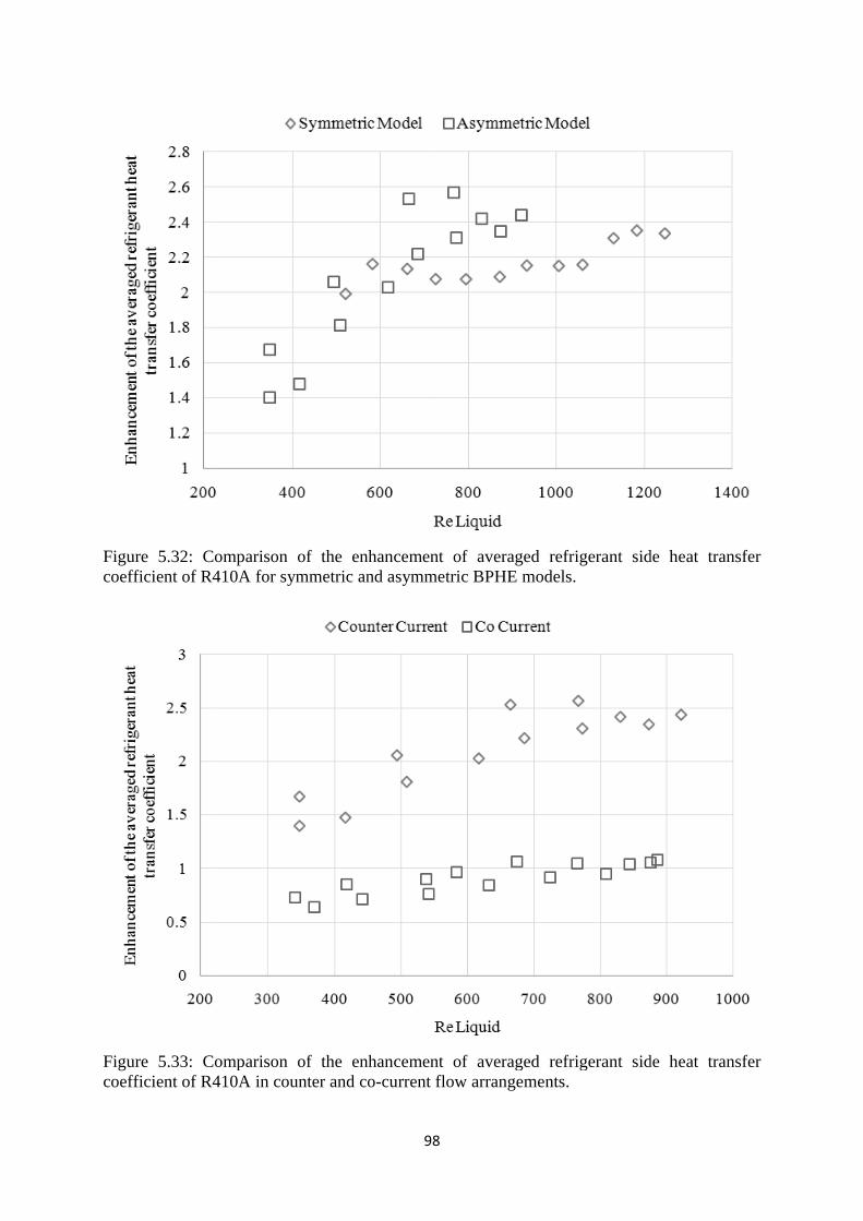
Figure 5.32: Comparison of the enhancement of averaged refrigerant side heat transfer coefficient of R410A for symmetric and asymmetric BPHE models.

Figure 5.33: Comparison of the enhancement of averaged refrigerant side heat transfer coefficient of R410A in counter and co

98

: Comparison of the enhancement of averaged refrigerant side heat transfer efficient of R410A for symmetric and asymmetric BPHE models.

: Comparison of the enhancement of averaged refrigerant side heat transfer coefficient of R410A in counter and co-current flow arrangements.

98

: Comparison of the enhancement of averaged refrigerant side heat transfer efficient of R410A for symmetric and asymmetric BPHE models.

: Comparison of the enhancement of averaged refrigerant side heat transfer current flow arrangements.

: Comparison of the enhancement of averaged refrigerant side heat transfer

: Comparison of the enhancement of averaged refrigerant side heat transfer

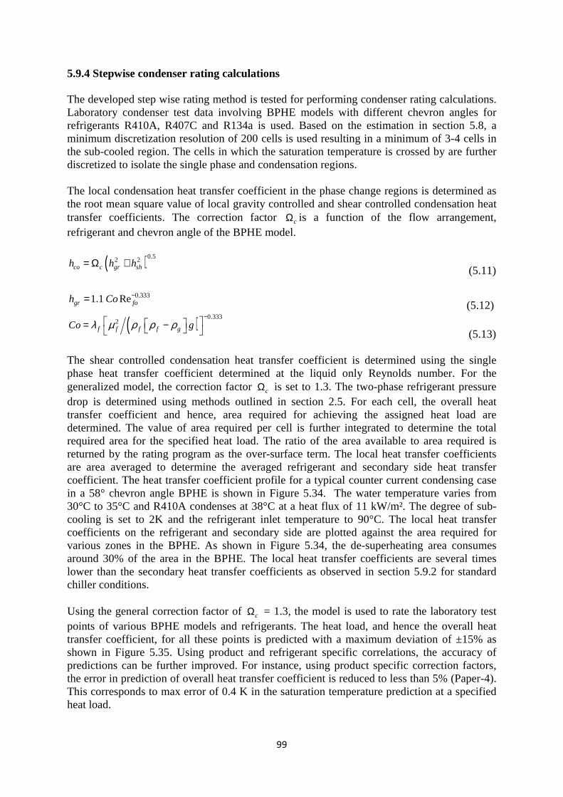
99

5.9.4 Stepwise condenser rating calculations The developed step wise rating method is tested for performing condenser rating calculations. Laboratory condenser test data involving BPHE models with different chevron angles for refrigerants R410A, R407C and R134a is used. Based on the estimation in section 5.8, a minimum discretization resolution of 200 cells is used resulting in a minimum of 3-4 cells in the sub-cooled region. The cells in which the saturation temperature is crossed by are further discretized to isolate the single phase and condensation regions. The local condensation heat transfer coefficient in the phase change regions is determined as the root mean square value of local gravity controlled and shear controlled condensation heat transfer coefficients. The correction factor cΩ is a function of the flow arrangement, refrigerant and chevron angle of the BPHE model.

( )0.52 2co c gr shh h h= Ω +

(5.11)

0.3331.1 Regr foh Co −= (5.12)

( ) 0.3332

f f f f gCo gλ µ ρ ρ ρ−

= − (5.13)

The shear controlled condensation heat transfer coefficient is determined using the single phase heat transfer coefficient determined at the liquid only Reynolds number. For the generalized model, the correction factor cΩ is set to 1.3. The two-phase refrigerant pressure drop is determined using methods outlined in section 2.5. For each cell, the overall heat transfer coefficient and hence, area required for achieving the assigned heat load are determined. The value of area required per cell is further integrated to determine the total required area for the specified heat load. The ratio of the area available to area required is returned by the rating program as the over-surface term. The local heat transfer coefficients are area averaged to determine the averaged refrigerant and secondary side heat transfer coefficient. The heat transfer coefficient profile for a typical counter current condensing case in a 58° chevron angle BPHE is shown in Figure 5.34. The water temperature varies from 30°C to 35°C and R410A condenses at 38°C at a heat flux of 11 kW/m². The degree of sub-cooling is set to 2K and the refrigerant inlet temperature to 90°C. The local heat transfer coefficients on the refrigerant and secondary side are plotted against the area required for various zones in the BPHE. As shown in Figure 5.34, the de-superheating area consumes around 30% of the area in the BPHE. The local heat transfer coefficients are several times lower than the secondary heat transfer coefficients as observed in section 5.9.2 for standard chiller conditions. Using the general correction factor of cΩ = 1.3, the model is used to rate the laboratory test points of various BPHE models and refrigerants. The heat load, and hence the overall heat transfer coefficient, for all these points is predicted with a maximum deviation of ±15% as shown in Figure 5.35. Using product and refrigerant specific correlations, the accuracy of predictions can be further improved. For instance, using product specific correction factors, the error in prediction of overall heat transfer coefficient is reduced to less than 5% (Paper-4). This corresponds to max error of 0.4 K in the saturation temperature prediction at a specified heat load.

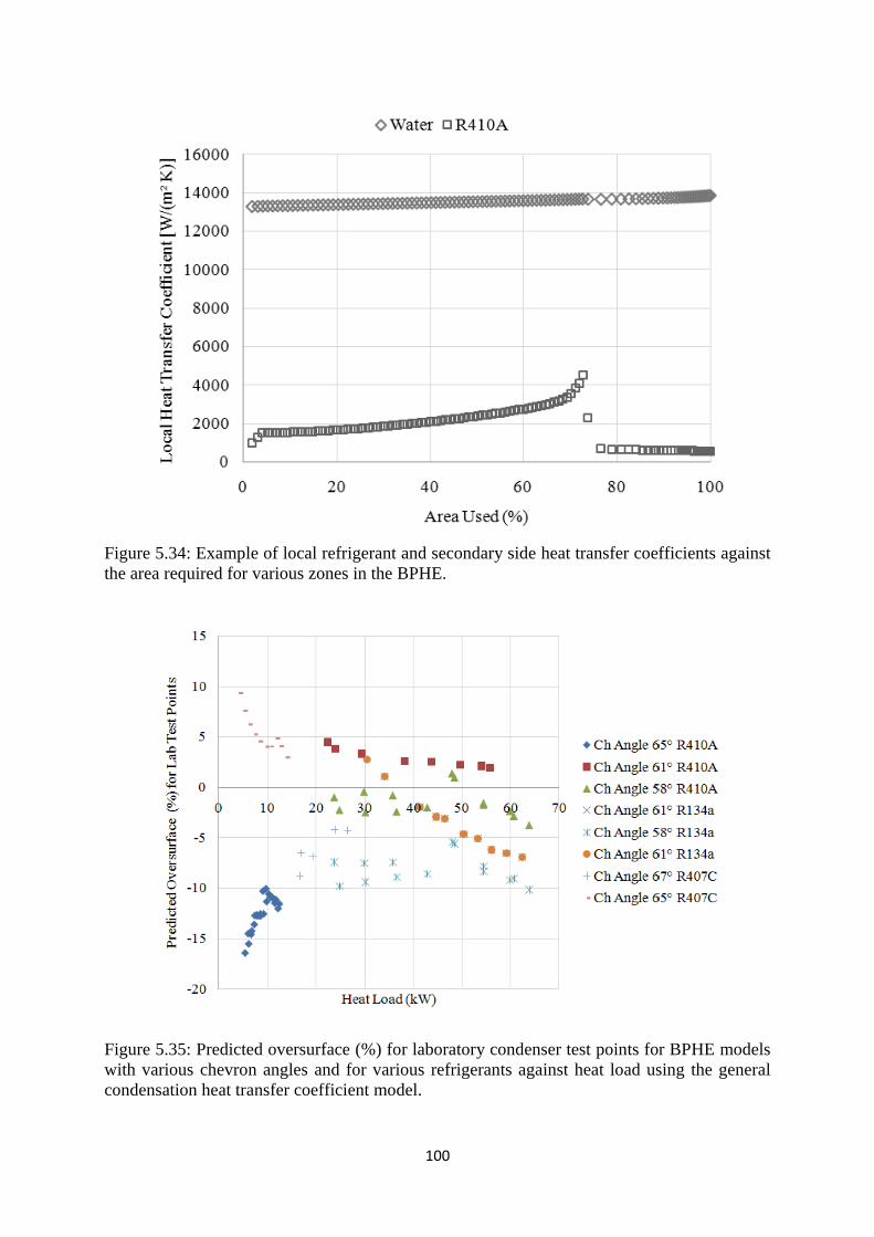
Figure 5.34: Example of local refrigerant and secondary side heat transfer coefficients against the area required for various zones in the BPHE.

Figure 5.35: Predicted with various chevron angles and for various refrigerants against heat load using the general condensation heat transfer coefficient

100

: Example of local refrigerant and secondary side heat transfer coefficients against the area required for various zones in the BPHE.

: Predicted oversurface (%) for laboratory condenser test points for BPHE models with various chevron angles and for various refrigerants against heat load using the general condensation heat transfer coefficient model.

100

: Example of local refrigerant and secondary side heat transfer coefficients against the area required for various zones in the BPHE.

oversurface (%) for laboratory condenser test points for BPHE models with various chevron angles and for various refrigerants against heat load using the general

: Example of local refrigerant and secondary side heat transfer coefficients against

oversurface (%) for laboratory condenser test points for BPHE models with various chevron angles and for various refrigerants against heat load using the general

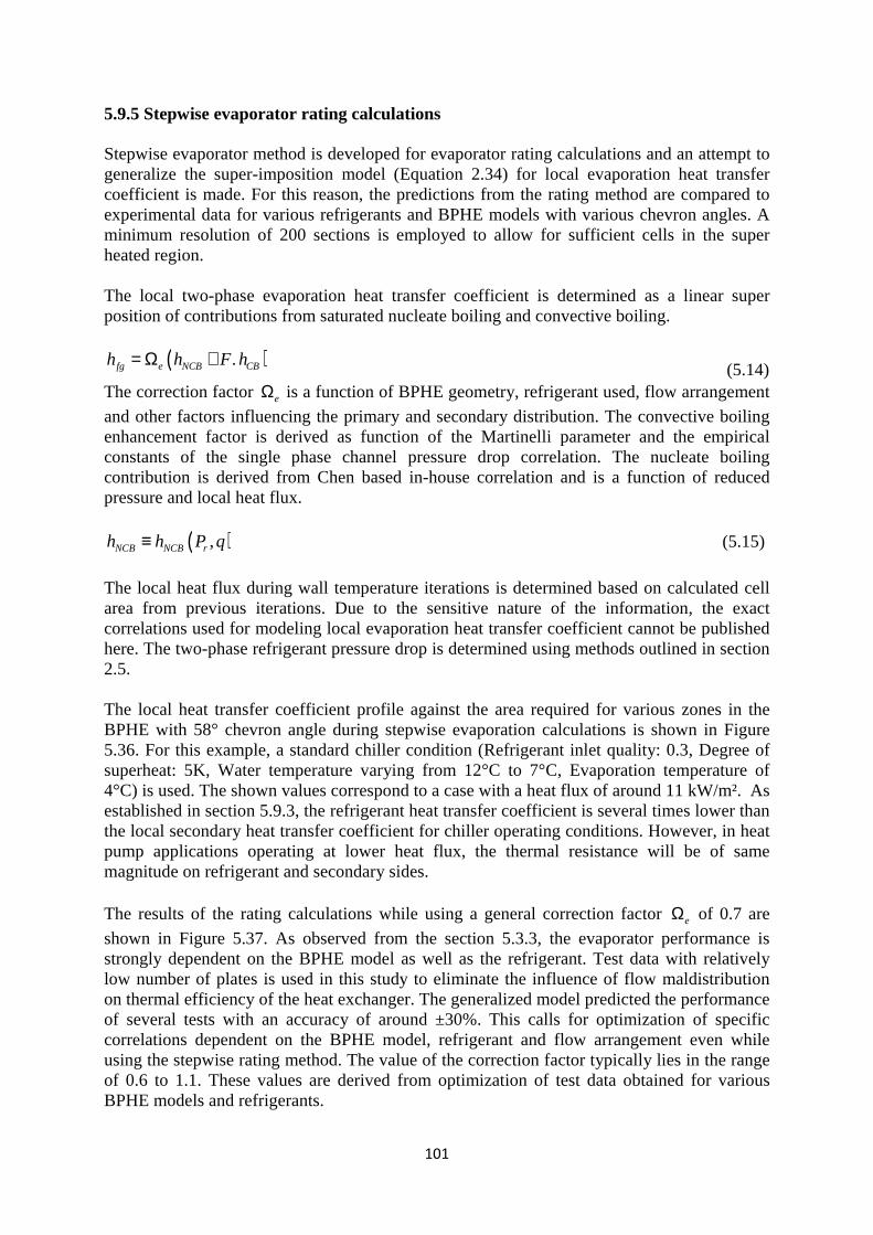
101

5.9.5 Stepwise evaporator rating calculations Stepwise evaporator method is developed for evaporator rating calculations and an attempt to generalize the super-imposition model (Equation 2.34) for local evaporation heat transfer coefficient is made. For this reason, the predictions from the rating method are compared to experimental data for various refrigerants and BPHE models with various chevron angles. A minimum resolution of 200 sections is employed to allow for sufficient cells in the super heated region. The local two-phase evaporation heat transfer coefficient is determined as a linear super position of contributions from saturated nucleate boiling and convective boiling.

( ).fg e NCB CBh h F h= Ω + (5.14)

The correction factor eΩ is a function of BPHE geometry, refrigerant used, flow arrangement

and other factors influencing the primary and secondary distribution. The convective boiling enhancement factor is derived as function of the Martinelli parameter and the empirical constants of the single phase channel pressure drop correlation. The nucleate boiling contribution is derived from Chen based in-house correlation and is a function of reduced pressure and local heat flux.

( ),NCB NCB rh h P q≡ (5.15)

The local heat flux during wall temperature iterations is determined based on calculated cell area from previous iterations. Due to the sensitive nature of the information, the exact correlations used for modeling local evaporation heat transfer coefficient cannot be published here. The two-phase refrigerant pressure drop is determined using methods outlined in section 2.5. The local heat transfer coefficient profile against the area required for various zones in the BPHE with 58° chevron angle during stepwise evaporation calculations is shown in Figure 5.36. For this example, a standard chiller condition (Refrigerant inlet quality: 0.3, Degree of superheat: 5K, Water temperature varying from 12°C to 7°C, Evaporation temperature of 4°C) is used. The shown values correspond to a case with a heat flux of around 11 kW/m². As established in section 5.9.3, the refrigerant heat transfer coefficient is several times lower than the local secondary heat transfer coefficient for chiller operating conditions. However, in heat pump applications operating at lower heat flux, the thermal resistance will be of same magnitude on refrigerant and secondary sides. The results of the rating calculations while using a general correction factor eΩ of 0.7 are

shown in Figure 5.37. As observed from the section 5.3.3, the evaporator performance is strongly dependent on the BPHE model as well as the refrigerant. Test data with relatively low number of plates is used in this study to eliminate the influence of flow maldistribution on thermal efficiency of the heat exchanger. The generalized model predicted the performance of several tests with an accuracy of around ±30%. This calls for optimization of specific correlations dependent on the BPHE model, refrigerant and flow arrangement even while using the stepwise rating method. The value of the correction factor typically lies in the range of 0.6 to 1.1. These values are derived from optimization of test data obtained for various BPHE models and refrigerants.

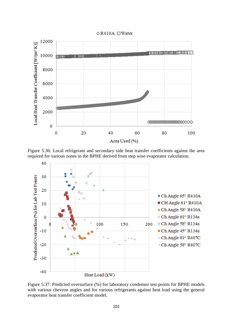
Figure 5.36: Local refrigerant and secondary side required for various zones in the BPHE derived from step wise evaporator calculation.

Figure 5.37: Predicted oversurface (%) for laboratory condenser test points for BPHE models with various chevron angles and evaporator heat transfer coefficient

102

: Local refrigerant and secondary side required for various zones in the BPHE derived from step wise evaporator calculation.

: Predicted oversurface (%) for laboratory condenser test points for BPHE models with various chevron angles and for various refrigerants against heat load using the general evaporator heat transfer coefficient model.

102

: Local refrigerant and secondary side heat transfer coefficients against the area required for various zones in the BPHE derived from step wise evaporator calculation.

: Predicted oversurface (%) for laboratory condenser test points for BPHE models for various refrigerants against heat load using the general

heat transfer coefficients against the area

required for various zones in the BPHE derived from step wise evaporator calculation.

: Predicted oversurface (%) for laboratory condenser test points for BPHE models

for various refrigerants against heat load using the general

103

5.10 DISCUSSION The application of developed step wise rating for single phase, condenser and evaporator calculations is presented. Test methodology employed for obtaining single phase and two-phase test data is briefly mentioned. Generalized single phase thermal and hydraulic correlations developed as function of flow conditions and BPHE dimensions can be used effectively for prediction of virtual products with a safety margin of 15%. However, improvement for these generalized correlation are required for asymmetric models and non-chevron pattern plate designs. Additional correction factors are required for multi-pass arrangements. Stepwise rating method improved the calculations with largely varying fluid properties. Due to its generality, the same calculation routines are successfully used for single phase, transcritical, evaporation, condensation and cascaded applications. Condenser and evaporation applications call for product, refrigerant and flow arrangement specific correction factors for determining local two-phase heat transfer coefficients.

REFERENCES Cavallini, A., Properties of CO2 as a refrigerant, European Seminar – Carbon dioxide as a refrigerant, Milan, 2004 Corradi, M., Cecchinato, L., Schiochet, G., Zilio, C., Modeling fin-and-tube gas cooler for transcritical carbon dioxide cycles (Paper ID 761), International Refrigeration and Air Conditioning Conference at Purdue, July 17-20, 2006 Martinez, S.M., Corberan, J. M., Gonzalvez, J. M., Domanski, P. A., Analysis of segment-by-segment ε-NTU modeling of a mini channel CO2 gas cooler (Paper ID 1033), International Refrigeration and Air Conditioning Conference at Purdue, July 12-15, 2010 Moffat, R.J., Contribution to the theory of single sample uncertainty analysis, Transactions of ASME, Journal of Fluids Engineering (104), pp 250-260, 1982. Nekså, P., Walnum, H. T., Hafner, A., CO2 – A refrigerant from the past with properties of being one of the main refrigerant in the future, 9th IIR Gustav Lorentzen Conference 2010 – natural refrigerants – real alternatives, Sydney, April 12-14, 2010. Pacheco-Vega, A. J., Simulation of compact heat exchangers using global regression and soft computing, Dissertation for the Degree of Doctor of Philosophy, Department of Aerospace and Mechanical Engineering, University of Notre Dame, April 2002. Palmer, S.C., Evaporation and condensation heat transfer performance of flammable refrigerants in brazed plate heat exchanger, NIST, NIST IR 6541 Sarkar, J., Bhattacharyya, S., Ram Gopal, M., Optimization of a transcritical CO2 heat pump cycle for simultaneous cooling and heating applications, International Journal of Refrigeration, Volume 27, pp. 830-838, 2004 Wang, L., Sundén, B., and Manglik, R.M., Plate Heat Exchangers: Design, Applications and Performance, WIT Press, ISBN 978-1-85312-737-3, 2007.

104

Yamasaki, H., Yamanaka, M., Matsumoto, K., Shimada, G., Introduction of transcritical refrigeration cycle utilizing CO2 as working fluid (Paper ID 1632), International Compressor Engineering Conference at Purdue, July 12-15, 2004

105

6.0 CONCLUDING REMARKS

6.1 CONCLUSIONS The current work aimed at exploring various methods of thermal and hydraulic performance estimation of compact brazed heat exchangers operating in several applications. Simplified, fast and order reduced modeling techniques are required for modeling BPHEs in selection software and in refrigeration system simulation programs. An attempt was made during the pre-study of this thesis work (Gullapalli 2008) to model the BPHEs as fluid systems. That method facilitated the modeling of complex flow paths with fluid elements extended between nodes. The fluid elements were characterized by the flow rate and pressure drop whereas the nodes were characterized by local enthalpy and pressure. The 1D finite volume approach was successful in modeling complex flow arrangements, multi-stream arrangements and to some extent the flow maldistribution in BPHEs. However, due to computational limitations, such a model could not be successfully implemented in BPHE selection software. In the current study, a further simplified, yet continuous, general and robust rating method is developed for implementation in BPHE selection software. The pressure-enthalpy based method is general and the same calculation framework can be used for all applications. The developed model is chosen to be a rating model (all boundary temperature specified). This improved the stability and improved the convergence characteristics of the iterative calculations. The sub routines used for single phase and phase change thermal and hydraulic correlations are chosen to be continuous. High degree of accuracy is achieved by using simplified and continuous correlations and product specific correction factors. However, being a 1D model, additional correction factors are required to handle multi-pass flow arrangements, maldistribution in refrigerant and secondary sides, cross flow arrangement and other influential factors. The suitability of the developed method for various single phase applications, transcritical CO2 calculations, condenser calculations, evaporator calculations are presented in the previous chapters. The developed method is currently implemented in SWEP BPHE selection software for transcritical CO2 calculations and cascaded BPHE calculations. Currently, work is ongoing to extend the developed method for condenser and evaporator rating calculations. A new finite grid interpolation based method is developed for fast and accurate retrieval of fluid properties. The method involves creating property maps in pressure enthalpy domain based on standard databases as NIST REFPROP. These data maps can then be used for determining fluid properties by local finite element interpolation (resulting in first order continuous properties). Using efficient data structures and indexing, excellent speed is achieved in fluid property retrieval. The size of the data maps are optimized aiming at a maximum deviation of 1% from standard databases. Several other calculation software applications are developed during the thesis work for dealing with requirements such as data import/ export, data visualization, curve fitting using non linear regression and single objective optimization. Software for single phase and two-phase test data evaluation is developed which employs various search techniques and meta-heuristic techniques for determining empirical constants in product specific thermal and hydraulic correlations. The generalized single phase thermal and hydraulic correlations were developed using non-linear regression technique.

106

The suitability of using commercial computational fluid dynamics (CFD) codes for prediction of single phase thermal and hydraulic performance of plate heat exchangers is investigated. CFD based methods play a major role in new product development, particularly of modern non-chevron type, application oriented asymmetric plate patterns. In the current work, a brief introduction to the governing equation of fluid flow, RANS turbulence models and near wall treatment is presented. Guidelines for fluid core and boundary meshing are presented based on mesh independent studies on channel fluid geometries. Various wall thermal boundary conditions are investigated and the simulations results are compared with experimental data and results from conjugate heat transfer simulations. Parametric studies on fluid sections characterized by various chevron angles are conducted and the results are compared with experimental data. The influence of choice of turbulence models is determined using simulation of entire channels. Furthermore, the visualization of flow patterns while using fluid sections having different chevron angles is also presented. The results observed for the condenser and evaporator calculations using the developed stepwise rating method suggests that the heat transfer and pressure drop in BPHEs could be predicted with reasonable accuracy using product specific correlations in the most commonly used operating conditions. Further work is required to calibrate models at very low Reynolds number conditions and during asymmetric loads in dual circuit heat exchangers. Investigations of CFD simulations showed that commercial CFD codes could be useful for determining relative performance variation of different plate designs and for improving plate designs for better in-channel flow distribution. REFERENCES Gullapalli, V.S., On Performance Analysis of Plate Heat Exchangers, Thesis for the Degree of Licentiate in Engineering, ISRN LUTMDN/TMHP-08/7055-SE, 2008

107

Paper 1

CFD Simulation of Heat Transfer and Pressure Drop in Compact Brazed Plate Heat Exchangers Submitted for publication to the Journal of Heat Transfer Engineering on June 7th 2012, Conditional acceptance received on February 28th, 2013. Full paper submission done on May 15th, 2013

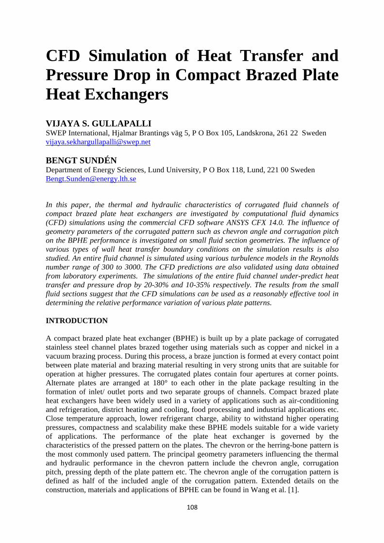
108

CFD Simulation of Heat Transfer and Pressure Drop in Compact Brazed Plate Heat Exchangers VIJAYA S. GULLAPALLI SWEP International, Hjalmar Brantings väg 5, P O Box 105, Landskrona, 261 22 Sweden vijaya.sekhargullapalli@swep.net

BENGT SUNDÉN Department of Energy Sciences, Lund University, P O Box 118, Lund, 221 00 Sweden Bengt.Sunden@energy.lth.se

In this paper, the thermal and hydraulic characteristics of corrugated fluid channels of compact brazed plate heat exchangers are investigated by computational fluid dynamics (CFD) simulations using the commercial CFD software ANSYS CFX 14.0. The influence of geometry parameters of the corrugated pattern such as chevron angle and corrugation pitch on the BPHE performance is investigated on small fluid section geometries. The influence of various types of wall heat transfer boundary conditions on the simulation results is also studied. An entire fluid channel is simulated using various turbulence models in the Reynolds number range of 300 to 3000. The CFD predictions are also validated using data obtained from laboratory experiments. The simulations of the entire fluid channel under-predict heat transfer and pressure drop by 20-30% and 10-35% respectively. The results from the small fluid sections suggest that the CFD simulations can be used as a reasonably effective tool in determining the relative performance variation of various plate patterns. INTRODUCTION A compact brazed plate heat exchanger (BPHE) is built up by a plate package of corrugated stainless steel channel plates brazed together using materials such as copper and nickel in a vacuum brazing process. During this process, a braze junction is formed at every contact point between plate material and brazing material resulting in very strong units that are suitable for operation at higher pressures. The corrugated plates contain four apertures at corner points. Alternate plates are arranged at 180° to each other in the plate package resulting in the formation of inlet/ outlet ports and two separate groups of channels. Compact brazed plate heat exchangers have been widely used in a variety of applications such as air-conditioning and refrigeration, district heating and cooling, food processing and industrial applications etc. Close temperature approach, lower refrigerant charge, ability to withstand higher operating pressures, compactness and scalability make these BPHE models suitable for a wide variety of applications. The performance of the plate heat exchanger is governed by the characteristics of the pressed pattern on the plates. The chevron or the herring-bone pattern is the most commonly used pattern. The principal geometry parameters influencing the thermal and hydraulic performance in the chevron pattern include the chevron angle, corrugation pitch, pressing depth of the plate pattern etc. The chevron angle of the corrugation pattern is defined as half of the included angle of the corrugation pattern. Extended details on the construction, materials and applications of BPHE can be found in Wang et al. [1].

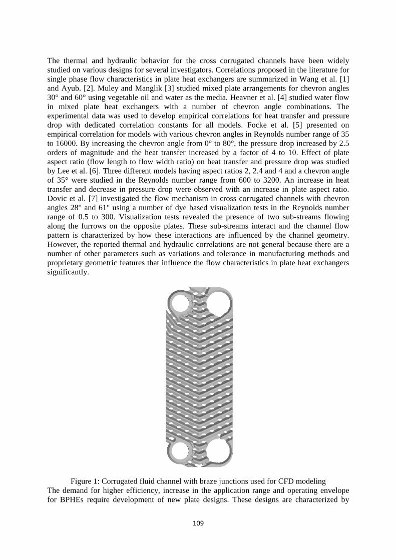
The thermal and hydraulic behavior for the cross corrugated channels have been widely studied on various designs for several investigators. Correlations proposed in the literature for single phase flow characteristics in plate heat exchangers are summarized in Wang et al. [1] and Ayub. [2]. Muley and Manglik [3] studied mixed plate arrangem30° and 60° using vegetable oil and water as the media. Heavner et al. [4] studied water flow in mixed plate heat exchangers with a number of chevron angle combinations. The experimental data was used to develop empirical correlatiodrop with dedicated correlation constants for all models. Focke et al. [5] presented on empirical correlation for models with various chevron angles in Reynolds number range of 35 to 16000. By increasing the chevron angle orders of magnitude and the heat transfer increased by a factor of 4 to 10. Effect of plate aspect ratio (flow length to flow width ratio) on heat transfer and pressure drop was studied by Lee et al. [6]. of 35° were studied in the Reynolds number range from 600 to 3200. An increase in heat transfer and decrease in pressure drop were observed with an increase in plate aspect ratio.Dovic et al. [7] investigated the flow mechanism in cross corrugated channels with chevron angles 28° and 61° using a number of dye based visualization tests in the Reynolds number range of 0.5 to 300. Visualization tests revealed the presence of two subalong the furrows on the opposite plates. These subpattern is characterized by how these interactions are influenced by the channel geometry. However, the reported thermal and hydraulic correlations arnumber of other parameters such as variations and tolerance in manufacturing methods and proprietary geometric features that influence the flow characteristics in plate heat exchangers significantly.

Figure 1: CorrugatThe demand for higher efficiency, increase in the application range and operating envelope for BPHEs require development of new plate designs. These designs are characterized by

109

The thermal and hydraulic behavior for the cross corrugated channels have been widely studied on various designs for several investigators. Correlations proposed in the literature for single phase flow characteristics in plate heat exchangers are summarized in Wang et al. [1] and Ayub. [2]. Muley and Manglik [3] studied mixed plate arrangem30° and 60° using vegetable oil and water as the media. Heavner et al. [4] studied water flow in mixed plate heat exchangers with a number of chevron angle combinations. The experimental data was used to develop empirical correlatiodrop with dedicated correlation constants for all models. Focke et al. [5] presented on empirical correlation for models with various chevron angles in Reynolds number range of 35 to 16000. By increasing the chevron angle from 0° to 80°, the pressure drop increased by 2.5 orders of magnitude and the heat transfer increased by a factor of 4 to 10. Effect of plate aspect ratio (flow length to flow width ratio) on heat transfer and pressure drop was studied by Lee et al. [6]. Three different models having aspect ratios 2, 2.4 and 4 and a chevron angle of 35° were studied in the Reynolds number range from 600 to 3200. An increase in heat transfer and decrease in pressure drop were observed with an increase in plate aspect ratio.Dovic et al. [7] investigated the flow mechanism in cross corrugated channels with chevron angles 28° and 61° using a number of dye based visualization tests in the Reynolds number range of 0.5 to 300. Visualization tests revealed the presence of two subalong the furrows on the opposite plates. These subpattern is characterized by how these interactions are influenced by the channel geometry. However, the reported thermal and hydraulic correlations arnumber of other parameters such as variations and tolerance in manufacturing methods and proprietary geometric features that influence the flow characteristics in plate heat exchangers

Figure 1: Corrugated fluid channel with braze junctions used for CFD modeling

The demand for higher efficiency, increase in the application range and operating envelope for BPHEs require development of new plate designs. These designs are characterized by

109

The thermal and hydraulic behavior for the cross corrugated channels have been widely studied on various designs for several investigators. Correlations proposed in the literature for single phase flow characteristics in plate heat exchangers are summarized in Wang et al. [1] and Ayub. [2]. Muley and Manglik [3] studied mixed plate arrangements for chevron angles 30° and 60° using vegetable oil and water as the media. Heavner et al. [4] studied water flow in mixed plate heat exchangers with a number of chevron angle combinations. The experimental data was used to develop empirical correlations for heat transfer and pressure drop with dedicated correlation constants for all models. Focke et al. [5] presented on empirical correlation for models with various chevron angles in Reynolds number range of 35

from 0° to 80°, the pressure drop increased by 2.5 orders of magnitude and the heat transfer increased by a factor of 4 to 10. Effect of plate aspect ratio (flow length to flow width ratio) on heat transfer and pressure drop was studied

Three different models having aspect ratios 2, 2.4 and 4 and a chevron angle of 35° were studied in the Reynolds number range from 600 to 3200. An increase in heat transfer and decrease in pressure drop were observed with an increase in plate aspect ratio.Dovic et al. [7] investigated the flow mechanism in cross corrugated channels with chevron angles 28° and 61° using a number of dye based visualization tests in the Reynolds number range of 0.5 to 300. Visualization tests revealed the presence of two sub-streams flowing along the furrows on the opposite plates. These sub-streams interact and the channel flow pattern is characterized by how these interactions are influenced by the channel geometry. However, the reported thermal and hydraulic correlations are not general because there are a number of other parameters such as variations and tolerance in manufacturing methods and proprietary geometric features that influence the flow characteristics in plate heat exchangers

ed fluid channel with braze junctions used for CFD modelingThe demand for higher efficiency, increase in the application range and operating envelope for BPHEs require development of new plate designs. These designs are characterized by

The thermal and hydraulic behavior for the cross corrugated channels have been widely studied on various designs for several investigators. Correlations proposed in the literature for single phase flow characteristics in plate heat exchangers are summarized in Wang et al. [1]

ents for chevron angles 30° and 60° using vegetable oil and water as the media. Heavner et al. [4] studied water flow in mixed plate heat exchangers with a number of chevron angle combinations. The

ns for heat transfer and pressure drop with dedicated correlation constants for all models. Focke et al. [5] presented on empirical correlation for models with various chevron angles in Reynolds number range of 35

from 0° to 80°, the pressure drop increased by 2.5 orders of magnitude and the heat transfer increased by a factor of 4 to 10. Effect of plate aspect ratio (flow length to flow width ratio) on heat transfer and pressure drop was studied

Three different models having aspect ratios 2, 2.4 and 4 and a chevron angle of 35° were studied in the Reynolds number range from 600 to 3200. An increase in heat transfer and decrease in pressure drop were observed with an increase in plate aspect ratio. Dovic et al. [7] investigated the flow mechanism in cross corrugated channels with chevron angles 28° and 61° using a number of dye based visualization tests in the Reynolds number

streams flowing streams interact and the channel flow

pattern is characterized by how these interactions are influenced by the channel geometry. e not general because there are a

number of other parameters such as variations and tolerance in manufacturing methods and proprietary geometric features that influence the flow characteristics in plate heat exchangers

ed fluid channel with braze junctions used for CFD modeling The demand for higher efficiency, increase in the application range and operating envelope for BPHEs require development of new plate designs. These designs are characterized by

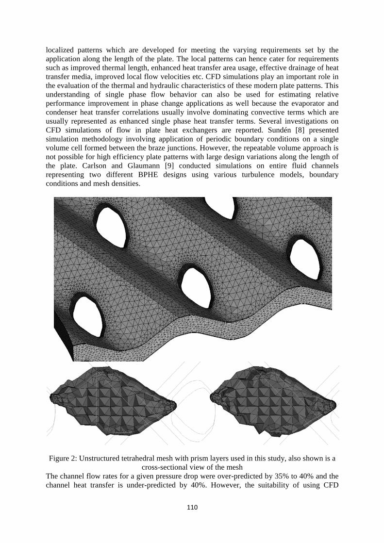
localized patternsapplication along the length of the plate. The local patterns can hence cater for requirements such as improved thermal length, enhanced heat transfer area usage, effective drainage of hetransfer media, improved local flow velocities etc. CFD simulations play an important role in the evaluation of the thermal and hydraulic characteristics of these modern plate patterns. This understanding of single phase flow behavior can also be used fperformance improvement in phase change applications as well because the evaporator and condenser heat transfer correlations usually involve dominating convective terms which are usually represented as enhanced single phase heat tranCFD simulations of flow in plate heat exchangers are reported. Sundén [8] presented simulation methodology involving application of periodic boundary conditions on a single volume cell formed between the braze junctionnot possible for high efficiency plate patterns with large design variations along the length of the plate. Carlson and Glaumann [9] conducted simulations on entire fluid channels representing two different BPHconditions and mesh densities.

Figure 2: Unstructured tetrahedral mesh with prism layers used in this study, also shown is a

The channel flow rates for a given preschannel heat transfer is under

110

localized patterns which are developed for meeting the varying requirements set by the application along the length of the plate. The local patterns can hence cater for requirements such as improved thermal length, enhanced heat transfer area usage, effective drainage of hetransfer media, improved local flow velocities etc. CFD simulations play an important role in the evaluation of the thermal and hydraulic characteristics of these modern plate patterns. This understanding of single phase flow behavior can also be used fperformance improvement in phase change applications as well because the evaporator and condenser heat transfer correlations usually involve dominating convective terms which are usually represented as enhanced single phase heat tranCFD simulations of flow in plate heat exchangers are reported. Sundén [8] presented simulation methodology involving application of periodic boundary conditions on a single volume cell formed between the braze junctions. However, the repeatable volume approach is not possible for high efficiency plate patterns with large design variations along the length of the plate. Carlson and Glaumann [9] conducted simulations on entire fluid channels representing two different BPHE designs using various turbulence models, boundary conditions and mesh densities.

Figure 2: Unstructured tetrahedral mesh with prism layers used in this study, also shown is a

cross-sectional view of the meshThe channel flow rates for a given pressure drop were overchannel heat transfer is under-predicted by 40%. However, the suitability of using CFD

110

which are developed for meeting the varying requirements set by the application along the length of the plate. The local patterns can hence cater for requirements such as improved thermal length, enhanced heat transfer area usage, effective drainage of hetransfer media, improved local flow velocities etc. CFD simulations play an important role in the evaluation of the thermal and hydraulic characteristics of these modern plate patterns. This understanding of single phase flow behavior can also be used for estimating relative performance improvement in phase change applications as well because the evaporator and condenser heat transfer correlations usually involve dominating convective terms which are usually represented as enhanced single phase heat transfer terms. Several investigations on CFD simulations of flow in plate heat exchangers are reported. Sundén [8] presented simulation methodology involving application of periodic boundary conditions on a single

s. However, the repeatable volume approach is not possible for high efficiency plate patterns with large design variations along the length of the plate. Carlson and Glaumann [9] conducted simulations on entire fluid channels

E designs using various turbulence models, boundary

Figure 2: Unstructured tetrahedral mesh with prism layers used in this study, also shown is a

sectional view of the mesh sure drop were over-predicted by 35% to 40% and the

predicted by 40%. However, the suitability of using CFD

which are developed for meeting the varying requirements set by the application along the length of the plate. The local patterns can hence cater for requirements such as improved thermal length, enhanced heat transfer area usage, effective drainage of heat transfer media, improved local flow velocities etc. CFD simulations play an important role in the evaluation of the thermal and hydraulic characteristics of these modern plate patterns. This

or estimating relative performance improvement in phase change applications as well because the evaporator and condenser heat transfer correlations usually involve dominating convective terms which are

sfer terms. Several investigations on CFD simulations of flow in plate heat exchangers are reported. Sundén [8] presented simulation methodology involving application of periodic boundary conditions on a single

s. However, the repeatable volume approach is not possible for high efficiency plate patterns with large design variations along the length of the plate. Carlson and Glaumann [9] conducted simulations on entire fluid channels

E designs using various turbulence models, boundary

Figure 2: Unstructured tetrahedral mesh with prism layers used in this study, also shown is a

predicted by 35% to 40% and the predicted by 40%. However, the suitability of using CFD

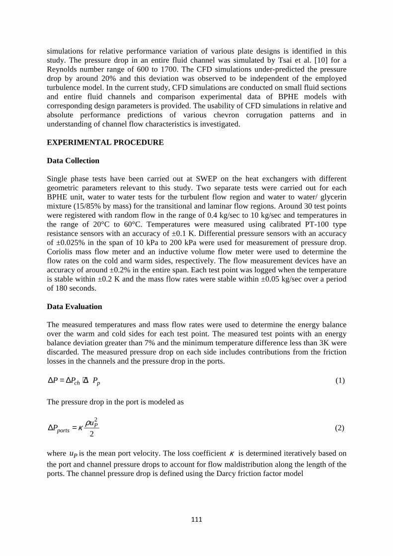
111

simulations for relative performance variation of various plate designs is identified in this study. The pressure drop in an entire fluid channel was simulated by Tsai et al. [10] for a Reynolds number range of 600 to 1700. The CFD simulations under-predicted the pressure drop by around 20% and this deviation was observed to be independent of the employed turbulence model. In the current study, CFD simulations are conducted on small fluid sections and entire fluid channels and comparison experimental data of BPHE models with corresponding design parameters is provided. The usability of CFD simulations in relative and absolute performance predictions of various chevron corrugation patterns and in understanding of channel flow characteristics is investigated. EXPERIMENTAL PROCEDURE Data Collection Single phase tests have been carried out at SWEP on the heat exchangers with different geometric parameters relevant to this study. Two separate tests were carried out for each BPHE unit, water to water tests for the turbulent flow region and water to water/ glycerin mixture (15/85% by mass) for the transitional and laminar flow regions. Around 30 test points were registered with random flow in the range of 0.4 kg/sec to 10 kg/sec and temperatures in the range of 20°C to 60°C. Temperatures were measured using calibrated PT-100 type resistance sensors with an accuracy of ±0.1 K. Differential pressure sensors with an accuracy of ±0.025% in the span of 10 kPa to 200 kPa were used for measurement of pressure drop. Coriolis mass flow meter and an inductive volume flow meter were used to determine the flow rates on the cold and warm sides, respectively. The flow measurement devices have an accuracy of around ±0.2% in the entire span. Each test point was logged when the temperature is stable within ±0.2 K and the mass flow rates were stable within ±0.05 kg/sec over a period of 180 seconds. Data Evaluation The measured temperatures and mass flow rates were used to determine the energy balance over the warm and cold sides for each test point. The measured test points with an energy balance deviation greater than 7% and the minimum temperature difference less than 3K were discarded. The measured pressure drop on each side includes contributions from the friction losses in the channels and the pressure drop in the ports.

ch pP P P∆ = ∆ + ∆ (1)

The pressure drop in the port is modeled as

2

2P

portsu

Pρκ∆ = (2)

where Pu is the mean port velocity. The loss coefficient κ is determined iteratively based on

the port and channel pressure drops to account for flow maldistribution along the length of the ports. The channel pressure drop is defined using the Darcy friction factor model

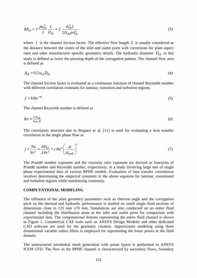
112

2 2

22 2ch ch

chch ch ch

u m LLP f f

D D A

ρρ

∆ = =ɺ

(3)

where f is the channel friction factor. The effective flow length L is usually considered as the distance between the centre of the inlet and outlet ports with corrections for plate aspect ratio and other manufacturer specific geometric details. The hydraulic diameter chD in this

study is defined as twice the pressing depth of the corrugation pattern. The channel flow area is defined as

0.5ch ch chA w D= (4)

The channel friction factor is evaluated as a continuous function of channel Reynolds number with different correlation constants for laminar, transition and turbulent regions.

Re mf b −= (5) The channel Reynolds number is defined as

2Re mchwch µ= ɺ

(6)

The correlation structure due to Bogaert et al. [11] is used for evaluating a heat transfer correlation in the single phase flow as

RePr Pr

znch

y ywall

hDNuj c

µµλ

= = =

(7)

The Prandtl number exponent and the viscosity ratio exponent are derived as functions of Prandtl number and Reynolds number, respectively, in a study involving large sets of single phase experimental data of various BPHE models. Evaluation of heat transfer correlations involves determining the empirical constants in the above equation for laminar, transitional and turbulent regions while maintaining continuity. COMPUTATIONAL MODELING The influence of the plate geometry parameters such as chevron angle and the corrugation pitch on the thermal and hydraulic performance is studied on small single fluid sections of dimensions close to 125 mm x70 mm. Simulations are also conducted on an entire fluid channel including the distribution areas at the inlet and outlet ports for comparison with experimental data. The computational domain representing the entire fluid channel is shown in Figure 1. Commercial CAE tools such as ANSYS Design Modeler and other dedicated CAD software are used for the geometry creation. Approximate modeling using three dimensional variable radius fillets is employed for representing the braze points in the fluid domain. The unstructured tetrahedral mesh generation with prism layers is performed in ANSYS ICEM CFD. The flow in the BPHE channel is characterized by secondary flows, boundary

113

layer separation and fluid stream interaction in the volumes available between the braze junctions. Features of the fluid channel such as corrugation crests, corrugations faces and braze junction surfaces are grouped into different regions for application of varying mesh dimensions in order to represent the actual flow conditions in a better manner. The requirement of the near wall mesh resolution is represented using a non-dimensional length

scaley+ . A y+ value of less than 2 is maintained for all the meshes in this study. An example of the surface mesh and the corresponding volume cell distribution in the channel cross section is shown in Figure 2. Mesh independency study for BPHE fluid sections was conducted by Gullapalli [12]. Various meshes with varying tetrahedral sizes and number of prism layers were developed in fluid section of dimensions 80.5 mm x 43 mm. CFD simulations with shear stress transport turbulence model in the Reynolds number range from 450 to 1800 were conducted. Stable results were obtained when the maximum tetra size was set to 1/7th of the corrugation pitch using five prism layers. A maximum surface deviation of 0.05 mm is recommended for all features in the fluid channel. The current simulation uses similar mesh resolution for the corrugation faces. A maximum element size of 0.1 mm is chosen for the braze junction surfaces for obtaining better mesh quality at the walls. A growth ratio of 1.1 is used for the prism layer with the cells in the last prism layer having similar volume as the adjacent tetrahedral cells. Simulations are carried out in ANSYS CFX 14.0 program setting the flow as incompressible, constant property, steady state and turbulent. A turbulence intensity of 10% is used at the inlet for which the ratio of turbulent viscosity to bulk viscosity is set as 100. Three different turbulence models available in CFX are used for the simulation of flow in the full channel. The RNG k-ε model is a relatively inexpensive two-equation model defining the eddy viscosity as a function of turbulent kinetic energy and turbulent dissipation rate. The shear stress transport model (SST) with automatic wall function is a blend of the k-ε and k-ω and has improved accuracy at wall and free stream conditions. The Reynolds stress turbulence models (RSM) are based on the transport equations for all components of the Reynolds stress tensor and the dissipation rate. The models solve for the transport of Reynolds stresses in the fluid and do not use the eddy viscosity hypothesis. The Launder-Reece-Rodi Isotropization of Production (LRR-IP) Reynolds stress model is used in this study. It uses a specific algebraic relation for the pressure strain correlation. (ANSYS Inc, [13]) Uniform mass flow rate with constant static inlet temperature is specified at the inlet. Constant pressure boundary condition is used at the outlet of computational domain. The influence of employing various methods of specifying the wall boundary conditions is studied. Due to computational limitations, it is common to simulate a single fluid channel. This requires specification of constant wall temperature, constant heat flux or an external wall heat transfer coefficient with ambient temperature as the wall boundary condition. The prediction of the thermal performance using these methods is compared with studies on conjugate heat transfer simulations with fluid channels and a solid plate domain with stainless steel properties. All the simulations are conducted on a Windows HPC cluster with two computing nodes with Intel Xeon 2.67 GHz CPU and 100 GB of random access memory. RESULTS AND DISCUSSION Influence of Wall Boundary Conditions The influence of the choice of various heat transfer boundary conditions on the prediction of the thermal performance is studied in a fluid section of dimensions 80.5 mm x 58 mm. The

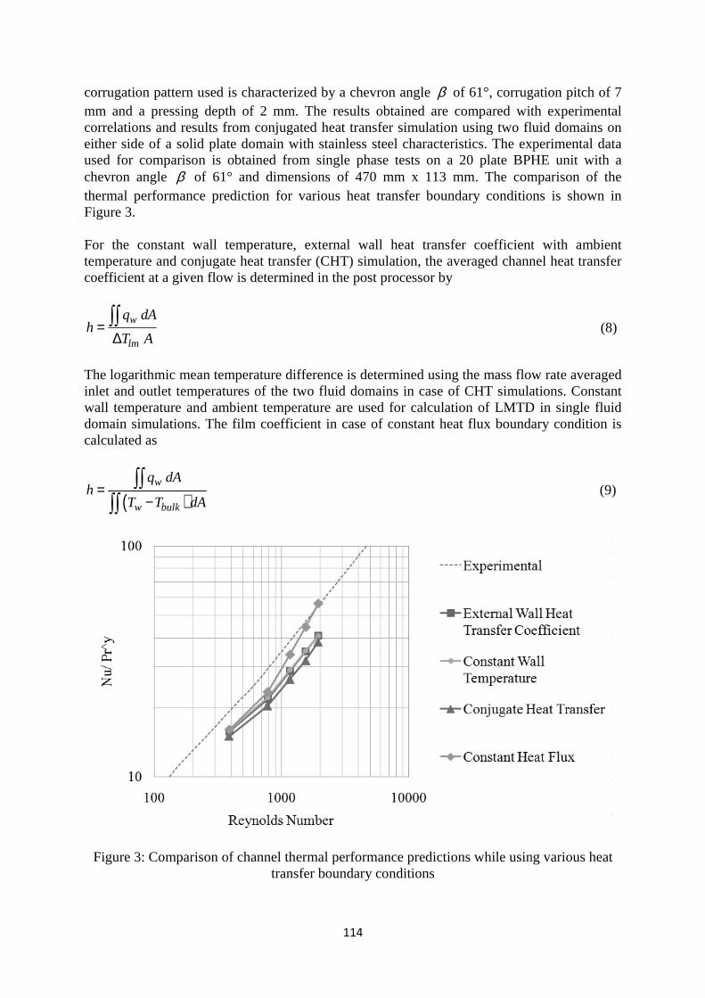
corrugation pattern used is characterized by a chevron angle mm and a pressing depth of 2 mm. The results obtained are compared with experimental correlations and results from conjugated heat transfer simulation using two fluid domains on either side of a solid plate domain with stainless steel characteristics. The experimeused for comparison is obtained from single phase tests on a 20 plate BPHE unit with a chevron angle βthermal performance prediction for various heat transfFigure 3. For the constant wall temperature, external wall heat transfer coefficient with ambient temperature and conjugate heat transfer (CHT) simulation, the averaged channel heat transfer coefficient at a given flow i

w

lm

q dAh

T A=

∆∫∫

The logarithmic mean temperature difference is determined inlet and outlet temperatures of the two fluid domains in case of CHT simulations. Constant wall temperature and ambient temperature are used for calculation of LMTD in single fluid domain simulations. The film coefficientcalculated as

(w

w bulk

q dAh

T T dA=

−∫∫

∫∫

Figure 3: Comparison of channel thermal

114

corrugation pattern used is characterized by a chevron angle pressing depth of 2 mm. The results obtained are compared with experimental

correlations and results from conjugated heat transfer simulation using two fluid domains on either side of a solid plate domain with stainless steel characteristics. The experimeused for comparison is obtained from single phase tests on a 20 plate BPHE unit with a

β of 61° and dimensions of 470 mm x 113 mm. The comparison of the thermal performance prediction for various heat transf

For the constant wall temperature, external wall heat transfer coefficient with ambient temperature and conjugate heat transfer (CHT) simulation, the averaged channel heat transfer coefficient at a given flow is determined in the post processor by

The logarithmic mean temperature difference is determined inlet and outlet temperatures of the two fluid domains in case of CHT simulations. Constant wall temperature and ambient temperature are used for calculation of LMTD in single fluid domain simulations. The film coefficient in case of constant heat flux boundary condition is

)w bulk

q dA

T T dA

∫∫

Figure 3: Comparison of channel thermal performance predictions while using various heat

transfer boundary conditions

114

corrugation pattern used is characterized by a chevron angle β of 61°, corrugation pitch of 7 pressing depth of 2 mm. The results obtained are compared with experimental

correlations and results from conjugated heat transfer simulation using two fluid domains on either side of a solid plate domain with stainless steel characteristics. The experimeused for comparison is obtained from single phase tests on a 20 plate BPHE unit with a

of 61° and dimensions of 470 mm x 113 mm. The comparison of the thermal performance prediction for various heat transfer boundary conditions is shown in

For the constant wall temperature, external wall heat transfer coefficient with ambient temperature and conjugate heat transfer (CHT) simulation, the averaged channel heat transfer

s determined in the post processor by

The logarithmic mean temperature difference is determined using the mass flow rate averaged inlet and outlet temperatures of the two fluid domains in case of CHT simulations. Constant wall temperature and ambient temperature are used for calculation of LMTD in single fluid

in case of constant heat flux boundary condition is

performance predictions while using various heat

transfer boundary conditions

of 61°, corrugation pitch of 7 pressing depth of 2 mm. The results obtained are compared with experimental

correlations and results from conjugated heat transfer simulation using two fluid domains on either side of a solid plate domain with stainless steel characteristics. The experimental data used for comparison is obtained from single phase tests on a 20 plate BPHE unit with a

of 61° and dimensions of 470 mm x 113 mm. The comparison of the er boundary conditions is shown in

For the constant wall temperature, external wall heat transfer coefficient with ambient temperature and conjugate heat transfer (CHT) simulation, the averaged channel heat transfer

(8)

using the mass flow rate averaged inlet and outlet temperatures of the two fluid domains in case of CHT simulations. Constant wall temperature and ambient temperature are used for calculation of LMTD in single fluid

in case of constant heat flux boundary condition is

(9)

performance predictions while using various heat

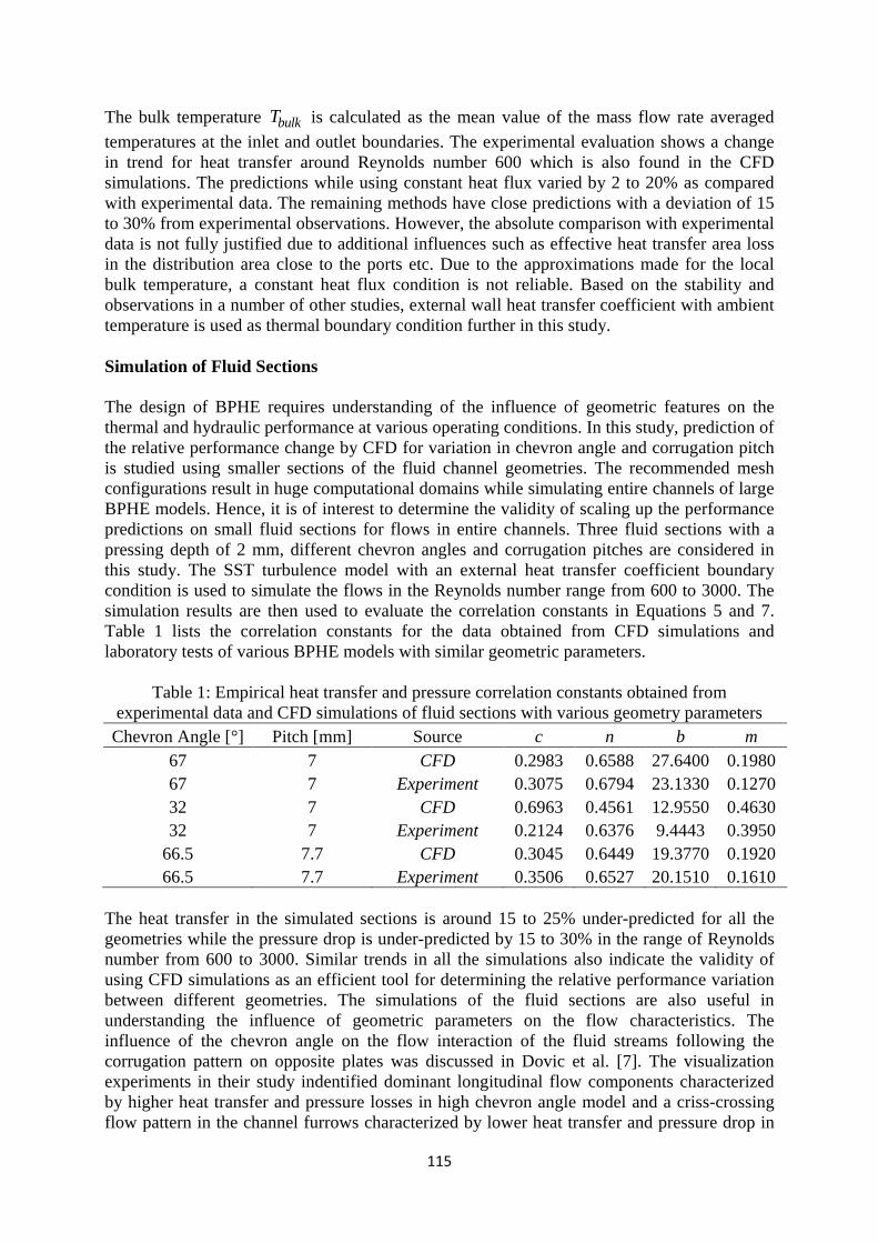
115

The bulk temperature bulkT is calculated as the mean value of the mass flow rate averaged

temperatures at the inlet and outlet boundaries. The experimental evaluation shows a change in trend for heat transfer around Reynolds number 600 which is also found in the CFD simulations. The predictions while using constant heat flux varied by 2 to 20% as compared with experimental data. The remaining methods have close predictions with a deviation of 15 to 30% from experimental observations. However, the absolute comparison with experimental data is not fully justified due to additional influences such as effective heat transfer area loss in the distribution area close to the ports etc. Due to the approximations made for the local bulk temperature, a constant heat flux condition is not reliable. Based on the stability and observations in a number of other studies, external wall heat transfer coefficient with ambient temperature is used as thermal boundary condition further in this study.

Simulation of Fluid Sections The design of BPHE requires understanding of the influence of geometric features on the thermal and hydraulic performance at various operating conditions. In this study, prediction of the relative performance change by CFD for variation in chevron angle and corrugation pitch is studied using smaller sections of the fluid channel geometries. The recommended mesh configurations result in huge computational domains while simulating entire channels of large BPHE models. Hence, it is of interest to determine the validity of scaling up the performance predictions on small fluid sections for flows in entire channels. Three fluid sections with a pressing depth of 2 mm, different chevron angles and corrugation pitches are considered in this study. The SST turbulence model with an external heat transfer coefficient boundary condition is used to simulate the flows in the Reynolds number range from 600 to 3000. The simulation results are then used to evaluate the correlation constants in Equations 5 and 7. Table 1 lists the correlation constants for the data obtained from CFD simulations and laboratory tests of various BPHE models with similar geometric parameters.

Table 1: Empirical heat transfer and pressure correlation constants obtained from experimental data and CFD simulations of fluid sections with various geometry parameters Chevron Angle [°] Pitch [mm] Source c n b m

67 7 CFD 0.2983 0.6588 27.6400 0.1980 67 7 Experiment 0.3075 0.6794 23.1330 0.1270 32 7 CFD 0.6963 0.4561 12.9550 0.4630 32 7 Experiment 0.2124 0.6376 9.4443 0.3950

66.5 7.7 CFD 0.3045 0.6449 19.3770 0.1920 66.5 7.7 Experiment 0.3506 0.6527 20.1510 0.1610

The heat transfer in the simulated sections is around 15 to 25% under-predicted for all the geometries while the pressure drop is under-predicted by 15 to 30% in the range of Reynolds number from 600 to 3000. Similar trends in all the simulations also indicate the validity of using CFD simulations as an efficient tool for determining the relative performance variation between different geometries. The simulations of the fluid sections are also useful in understanding the influence of geometric parameters on the flow characteristics. The influence of the chevron angle on the flow interaction of the fluid streams following the corrugation pattern on opposite plates was discussed in Dovic et al. [7]. The visualization experiments in their study indentified dominant longitudinal flow components characterized by higher heat transfer and pressure losses in high chevron angle model and a criss-crossing flow pattern in the channel furrows characterized by lower heat transfer and pressure drop in

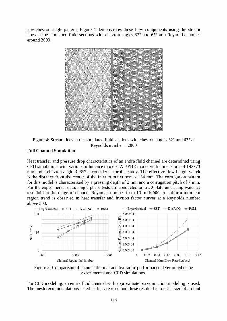
low chevron angle patlines in the simulated fluid sections with chevron angles 32° and 67° at a Reynolds number around 2000.

Figure 4: Stream lines in the simulated fluid sections with chevron angles 32° an

Full Channel Simulation Heat transfer and pressure drop characteristics of an entire fluid channel are determined using CFD simulations with various turbulence models. A BPHE model with dimensions of 192x73 mm and a chevronis the distance from the center of the inlet to outlet port is 154 mm. The corrugation pattern for this model is characterized by a pressing depth of 2 mm and a corrugation pitch ofFor the experimental data, single phase tests are conducted on a 20 plate unit using water as test fluid in the range of channel Reynolds number from 10 to 10000. A uniform turbulent region trend is observed in heat transfer and friction factor curabove 300.

Figure 5: Comparison of channel thermal and hydraulic performance determined using

For CFD modeling, an entire fluid channel with approximate braze junction modeling is used. The mesh recommendations listed earlier are used and these resulted in a mesh size of around

116

low chevron angle pattern. Figure 4 demonstrates these flow components using the stream lines in the simulated fluid sections with chevron angles 32° and 67° at a Reynolds number

Figure 4: Stream lines in the simulated fluid sections with chevron angles 32° an

Reynolds number Full Channel Simulation

Heat transfer and pressure drop characteristics of an entire fluid channel are determined using CFD simulations with various turbulence models. A BPHE model with dimensions of 192x73 mm and a chevron angle β=65° is considered for this study. The effective flow length which is the distance from the center of the inlet to outlet port is 154 mm. The corrugation pattern for this model is characterized by a pressing depth of 2 mm and a corrugation pitch ofFor the experimental data, single phase tests are conducted on a 20 plate unit using water as

in the range of channel Reynolds number from 10 to 10000. A uniform turbulent region trend is observed in heat transfer and friction factor cur

Figure 5: Comparison of channel thermal and hydraulic performance determined using experimental and CFD simulations.

For CFD modeling, an entire fluid channel with approximate braze junction modeling is used.

recommendations listed earlier are used and these resulted in a mesh size of around

116

tern. Figure 4 demonstrates these flow components using the stream lines in the simulated fluid sections with chevron angles 32° and 67° at a Reynolds number

Figure 4: Stream lines in the simulated fluid sections with chevron angles 32° anReynolds number ≈ 2000

Heat transfer and pressure drop characteristics of an entire fluid channel are determined using CFD simulations with various turbulence models. A BPHE model with dimensions of 192x73

β=65° is considered for this study. The effective flow length which is the distance from the center of the inlet to outlet port is 154 mm. The corrugation pattern for this model is characterized by a pressing depth of 2 mm and a corrugation pitch ofFor the experimental data, single phase tests are conducted on a 20 plate unit using water as

in the range of channel Reynolds number from 10 to 10000. A uniform turbulent region trend is observed in heat transfer and friction factor curves at a Reynolds number

Figure 5: Comparison of channel thermal and hydraulic performance determined using experimental and CFD simulations.

For CFD modeling, an entire fluid channel with approximate braze junction modeling is used.

recommendations listed earlier are used and these resulted in a mesh size of around

tern. Figure 4 demonstrates these flow components using the stream lines in the simulated fluid sections with chevron angles 32° and 67° at a Reynolds number

Figure 4: Stream lines in the simulated fluid sections with chevron angles 32° and 67° at

Heat transfer and pressure drop characteristics of an entire fluid channel are determined using CFD simulations with various turbulence models. A BPHE model with dimensions of 192x73

β=65° is considered for this study. The effective flow length which is the distance from the center of the inlet to outlet port is 154 mm. The corrugation pattern for this model is characterized by a pressing depth of 2 mm and a corrugation pitch of 7 mm. For the experimental data, single phase tests are conducted on a 20 plate unit using water as

in the range of channel Reynolds number from 10 to 10000. A uniform turbulent ves at a Reynolds number

Figure 5: Comparison of channel thermal and hydraulic performance determined using

For CFD modeling, an entire fluid channel with approximate braze junction modeling is used. recommendations listed earlier are used and these resulted in a mesh size of around

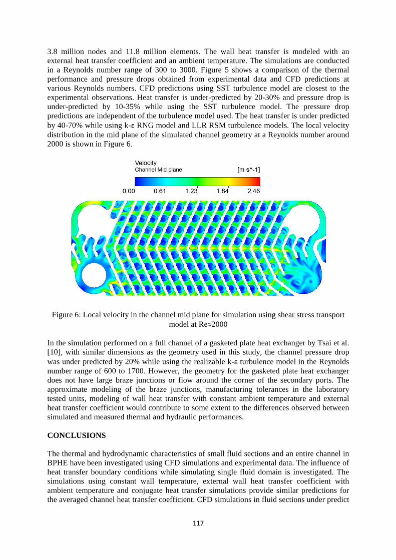
3.8 million nodes and 11.8 million elements. The wall heat transfer is modeled with an external heat transfer coefficient and an ambient temperature. The simulations are cin a Reynolds number range of 300 to 3000. Figure 5 shows a comparison of the thermal performance and pressure drops obtained from experimental data and CFD predictions at various Reynolds numbers. CFD predictions using SST turbulence model are clexperimental observations. Heat transfer is underunder-predicted by 10predictions are independent of the turbulence model used. The heat traby 40-70% while using kdistribution in the mid plane of the simulated channel geometry at a Reynolds number around 2000 is shown in Figure 6.

Figure 6: Local veloc

In the simulation performed on a full channel of a gasketed plate heat exchanger by Tsai et al. [10], with similar dimensions as the geometry used in this study, thewas under predicted by 20% while using the realizable knumber range of 600 to 1700. However, the geometry for the gasketed plate heat exchanger does not have large braze junctions or flow around thapproximate modeling of the braze junctions, manufacturing tolerances in the laboratory tested units, modeling of wall heat transfer with constant ambient temperature and external heat transfer coefficient would contribsimulated and measured thermal and hydraulic performances. CONCLUSIONS The thermal and hydrodynamic characteristics of small fluid sections and an entire channel in BPHE have been investigated usingheat transfer boundary conditions while simulating single fluid domain is investigated. The simulations using constant wall temperature, external wall heat transfer coefficient with ambient temperatuthe averaged channel heat transfer coefficient. CFD simulations in fluid sections under predict

117

3.8 million nodes and 11.8 million elements. The wall heat transfer is modeled with an external heat transfer coefficient and an ambient temperature. The simulations are cin a Reynolds number range of 300 to 3000. Figure 5 shows a comparison of the thermal performance and pressure drops obtained from experimental data and CFD predictions at various Reynolds numbers. CFD predictions using SST turbulence model are clexperimental observations. Heat transfer is under

predicted by 10-35% while using the SST turbulence model. The pressure drop predictions are independent of the turbulence model used. The heat tra

70% while using k-ε RNG model and LLR RSM turbulence models. The local velocity distribution in the mid plane of the simulated channel geometry at a Reynolds number around 2000 is shown in Figure 6.

Figure 6: Local velocity in the channel mid plane for simulation using shear stress transport

model at Re

In the simulation performed on a full channel of a gasketed plate heat exchanger by Tsai et al. [10], with similar dimensions as the geometry used in this study, thewas under predicted by 20% while using the realizable knumber range of 600 to 1700. However, the geometry for the gasketed plate heat exchanger does not have large braze junctions or flow around thapproximate modeling of the braze junctions, manufacturing tolerances in the laboratory tested units, modeling of wall heat transfer with constant ambient temperature and external heat transfer coefficient would contribute to some extent to the differences observed between simulated and measured thermal and hydraulic performances.

CONCLUSIONS

The thermal and hydrodynamic characteristics of small fluid sections and an entire channel in BPHE have been investigated using CFD simulations and experimental data. The influence of heat transfer boundary conditions while simulating single fluid domain is investigated. The simulations using constant wall temperature, external wall heat transfer coefficient with ambient temperature and conjugate heat transfer simulations provide similar predictions for the averaged channel heat transfer coefficient. CFD simulations in fluid sections under predict

117

3.8 million nodes and 11.8 million elements. The wall heat transfer is modeled with an external heat transfer coefficient and an ambient temperature. The simulations are cin a Reynolds number range of 300 to 3000. Figure 5 shows a comparison of the thermal performance and pressure drops obtained from experimental data and CFD predictions at various Reynolds numbers. CFD predictions using SST turbulence model are clexperimental observations. Heat transfer is under-predicted by 20-30% and pressure drop is

35% while using the SST turbulence model. The pressure drop predictions are independent of the turbulence model used. The heat transfer is under predicted

RNG model and LLR RSM turbulence models. The local velocity distribution in the mid plane of the simulated channel geometry at a Reynolds number around

ity in the channel mid plane for simulation using shear stress transport

model at Re≈2000

In the simulation performed on a full channel of a gasketed plate heat exchanger by Tsai et al. [10], with similar dimensions as the geometry used in this study, the channel pressure drop was under predicted by 20% while using the realizable k-ε turbulence model in the Reynolds number range of 600 to 1700. However, the geometry for the gasketed plate heat exchanger does not have large braze junctions or flow around the corner of the secondary ports. The approximate modeling of the braze junctions, manufacturing tolerances in the laboratory tested units, modeling of wall heat transfer with constant ambient temperature and external

ute to some extent to the differences observed between simulated and measured thermal and hydraulic performances.

The thermal and hydrodynamic characteristics of small fluid sections and an entire channel in CFD simulations and experimental data. The influence of

heat transfer boundary conditions while simulating single fluid domain is investigated. The simulations using constant wall temperature, external wall heat transfer coefficient with

re and conjugate heat transfer simulations provide similar predictions for the averaged channel heat transfer coefficient. CFD simulations in fluid sections under predict

3.8 million nodes and 11.8 million elements. The wall heat transfer is modeled with an external heat transfer coefficient and an ambient temperature. The simulations are conducted in a Reynolds number range of 300 to 3000. Figure 5 shows a comparison of the thermal performance and pressure drops obtained from experimental data and CFD predictions at various Reynolds numbers. CFD predictions using SST turbulence model are closest to the

30% and pressure drop is 35% while using the SST turbulence model. The pressure drop

nsfer is under predicted RNG model and LLR RSM turbulence models. The local velocity

distribution in the mid plane of the simulated channel geometry at a Reynolds number around

ity in the channel mid plane for simulation using shear stress transport

In the simulation performed on a full channel of a gasketed plate heat exchanger by Tsai et al. channel pressure drop

turbulence model in the Reynolds number range of 600 to 1700. However, the geometry for the gasketed plate heat exchanger

e corner of the secondary ports. The approximate modeling of the braze junctions, manufacturing tolerances in the laboratory tested units, modeling of wall heat transfer with constant ambient temperature and external

ute to some extent to the differences observed between

The thermal and hydrodynamic characteristics of small fluid sections and an entire channel in CFD simulations and experimental data. The influence of

heat transfer boundary conditions while simulating single fluid domain is investigated. The simulations using constant wall temperature, external wall heat transfer coefficient with

re and conjugate heat transfer simulations provide similar predictions for the averaged channel heat transfer coefficient. CFD simulations in fluid sections under predict

118

the heat transfer by 15-25% and pressure drop by 15-30%. This trend is commonly observed for all the simulated fluid sections suggesting that the CFD simulations are a reasonably effective tool in determining relative performance variation for various plate patterns. Furthermore, simulations of smaller fluid sections are useful for observing the flow interactions in the fluid channels. These simulations can be used to identify and correct bad geometric features which could result in enhancement of effective heat transfer area, local velocity profiles and distribution within the fluid channel. The full channel simulations using the shear stress transport turbulence model predict the heat transfer and pressure drop closest to the experimental data. For the entire channel simulations, the heat transfer is under predicted by 20-30% and the pressure drop by 10-35%. The choice of turbulence models has limited influence on the pressure drop predictions. High mesh resolutions containing 3 to 4 million nodes in the computational domain are used in all the simulations with each case requiring an average simulation time of 2 to 5 hours. In the current study, the braze junctions in the fluid sections are modeled approximately with variable radius fillets. Further improvement is required in the geometric representation of braze junctions for improving the accuracy of the CFD simulations. NOMENCLATURE A Cross sectional area or effective heat transfer area [m²] ,b c Empirical correlation constants

D Hydraulic diameter [m] f Channel friction factor h Convective heat transfer coefficient [W/(m²K)] j Dimensionless heat transfer group L Effective flow length [m]

,m n Empirical correlation constants Nu Nusselt number mɺ Channel mass flow rate [kg/sec] Pr Prandtl number q Wall heat flux [W/m²] Re Reynolds Number T Temperature [°C] u Velocity [m/sec] w Channel flow width [m] ,y z Empirical correlation constants

Greek Symbols β Chevron angle κ Loss coefficient for ports λ Fluid thermal conductivity [W/(m.K)] µ Dynamic viscosity [Pa sec] ρ Density [kg/m³]

P∆ Pressure drop [Pa] Subscripts

119

bulk Bulk conditions ch Channel lm Logarithmic mean p Ports w Wall REFERENCES [1] Wang, L., Sundén, B., and Manglik, R.M., Plate Heat Exchangers: Design, Applications and Performance, WIT Press, ISBN 978-1-85312-737-3, 2007. [2] Ayub, Z. H., Plate Heat Exchanger Literature Survey and New Heat Transfer and Pressure Drop Correlations for Refrigerant Evaporators, Heat Transfer Engineering, 24(5), pp. 3-16, 2003. [3] Muley. A., and Manglik, R.M., Enhanced Heat Transfer Characteristics of Single-Phase Flows in Plate Heat Exchangers with Mixed Chevron Plates, Journal of Enhanced Heat Transfer, Volume 3, pp. 187-201, 1997. [4] Heavner, R.L., Kumar, H., and Wanniarachchi, A.S., Performance of Industrial Plate Heat Exchanger: Effect of Chevron Angle, AIChE Symposium Series, Heat transfer – Atlanta 1993, Volume 89, No 295, pp. 262-267, 1993. [5] Focke, W. W., Zachariades, J., and Olivier, I., The Effect of the Corrugation Inclination Angle on the Thermohydraulic Performance of Plate Heat Exchangers, International Journal of Heat and Mass Transfer, Volume 28, No 8, pp. 1469-1479, 1985. [6] Lee. S. H, Cho. Y. I, Bai. C., and Cho. D. J., The effect of aspect ratio on turbulent flow heat transfer and pressure drop in plate heat exchanger, International Journal of Heat Exchangers, Volume 1, pp.113-124, 2000 [7] Dovic, D., Palm. B., and Svaic, S., Basic Single-Phase Flow Phenomena in Chevron-Type Plate Heat Exchangers, Zero Leakage – Minimum Charge, IIR/IIF, Stockholm, pp. 221-232, 2002 [8] Sundén, B., Computational fluid dynamics in research and design of heat exchangers, Heat Transfer Engineering, Volume 28, No 11, pp. 898-910, 2007 [9] Carlson. A., Glaumann. J., Simulation of heat transfer in compact brazed plate heat exchangers using CFD software Fluent, Master Thesis, Lund University, ISRN LUTMDN/TMHP-04/5034-SE ISSN 0282-1990, 2004 [10] Tsai Ying-Chi , Liu Fung-Bao, and Shen Po-Tsun., Investigations of the pressure drop and flow distribution in a chevron-type plate heat exchanger, International Communication in Heat and Mass Transfer 36: pp. 574-578, 2009 [11] Bogaert, R., Brazed Plate Heat Exchanger Project, Part 2: Thermal Characteristics of the Brazed Plate Heat Exchanger, Report LTT-94-06, Ecole Polytechnique Federale De Lausanne, 1994

120

[12] Gullapalli, V.S., Design of high efficiency compact brazed plate heat exchangers using CFD, Conference Proceedings Paper ID 614, The 23rd IIR International Conference of Refrigeration, Prague, August 21-26, 2011. [13] ANSYS Inc. ANSYS CFX-Solver Theory Guide, 2006

121

Paper 2

Design of high efficiency compact brazed plate heat exchangers using CFD Presented at the 23rd IIR International Congress of Refrigeration, Prague, Paper ID: 614

122

ID: 614

DESIGN OF HIGH EFFICIENCY COMPACT BRAZED PLATE HEAT EXCHANGERS USING CFD

GULLAPALLI, V.S (*) *SWEP International, Hjalmar Brantings väg 5, P O Box 105, Landskrona, 261 22 Sweden

vijaya.sekhargullapalli@swep.net

ABSTRACT

The design of plates used in compact brazed plate heat exchangers is traditionally performed by selection of geometric parameters suitable for meeting thermal and hydraulic requirements of a set of applications. The influence of each of the geometric parameters on heat transfer and pressure drop is generally available to the designer in form of equations obtained from laboratory and field tests. Geometry parameters such as chevron angle, pressing depth, corrugation wave length, plate aspect ratio, port diameters are usually optimized for the widely used herring bone plate pattern. In recent days, many high efficient plate patterns are developed which vary significantly in structure and flow characteristics compared to traditional corrugated plate patterns. The lack of generality in the definition of geometric parameters and variation in flow characteristics limit the use of aforementioned prediction equations for design of modern plate patterns. Commercial CFD codes are widely used in industry today for verifying the performance of new plate patterns in the design stage of new product development. However, this process is limited by issues such as complex and large CAD file handling, large geometry aspect ratios, approximation of features in fluid geometries and turbulence modeling. The current article discusses the choice of CFD parameters, such as mesh characteristics, turbulence models, boundary conditions etc on the accuracy of predictions. Examples where simple geometry changes resulted in significant improvement of performance are presented.

1. INTRODUCTION Compact brazed plate heat exchanges (BPHE) are built using a plate package of corrugated stainless steel channel plates brazed together with materials such as copper or nickel. During the vacuum brazing process, brazing points are formed at every contact point between the plates and braze materials. Plates are arranged in the plate package resulting in the alternate formation of hot and cold channels. Further information on the construction, materials and applications of BPHE can be found in, for example in Wang et al. (2007).

Figure 1. Plate and schematic of plate package in a compact brazed plate heat exchanger

The thermal and hydraulic performance of plate heat exchangers is influenced by plate geometry features such as chevron angle, pressing depth, corrugation pitch, plate thickness, port diameters etc. The influence of the individual parameters on performance is widely available in literature, for example, in Wang et al. (2007) and also in form of in-house correlations based on experimental data for commercial organizations. The design of heat exchangers for a given application usually involves choosing the appropriate geometry features which satisfy the desired thermal and hydraulic duty. The operating envelope, applications range and efficiency requirements are increasing rapidly for BPHEs. The standard design methodology is not applicable for design of BPHE in new operating envelopes

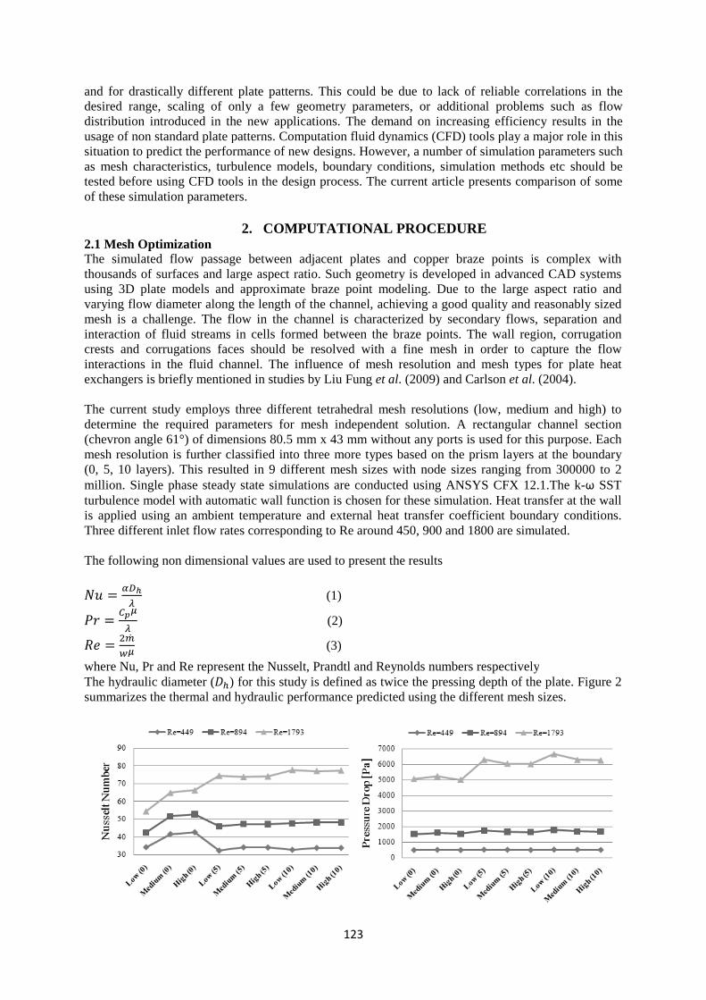
and for drastically different plate patterns. This could be due to lack of reliable correlations in the desired range, scaling of only a few geometry parameters, or additional problems such as flow distribution introduced in the new applications. The demand on increasing efficiency results in the usage of non standard plate patterns. Computation fluid dynamics (CFD) tsituation to predict the performance of new designs. However, a number of simulation parameters such as mesh characteristics, turbulence models, boundary conditions, simulation methods etc should be tested before using CFD toof these simulation parameters.

2.1 Mesh OptimizationThe simulated flow passage between adjacent plates and copper braze points is complex with thousands of surfaces and large aspect ratio. Such geometry is developed in advanced CAD systems using 3D plate models and approximate braze point modeling. Due to tvarying flow diameter along the length of the channel, achieving a good quality and reasonably sized mesh is a challenge. The flow in the channel is characterized by secondary flows, separation and interaction of fluid streams in crests and corrugations faces should be resolved with a fine mesh in order to capture the flow interactions in the fluid channel. The influence of mesh resolution and mesh types for plate exchangers is briefly mentioned in studies by Liu Fung The current study employs three different tetrahedral mesh resolutions (low, medium and high) to determine the required parameters for mesh independent so(chevron angle 61°) of dimensions 80.5 mm x 43 mm without any ports is used for this purpose. Each mesh resolution is further classified into three more types based on the prism layers at the boundary (0, 5, 10 layers). This resulted in 9 different mesh sizes with node sizes ranging from 300000 to 2 million. Single phase steady state simulations are conducted using ANSYS CFX 12.1.The kturbulence model with automatic wall function is chosen for these simulation. His applied using an ambient temperature and external heat transfer coefficient boundary conditions. Three different inlet flow rates corresponding to Re around 450, 900 and 1800 are simulated. The following non dimensional values

where Nu, Pr and Re represent the Nusselt, Prandtl and Reynolds numbers respectivelyThe hydraulic diameter (summarizes the thermal and hydraulic performance predicted using the different mesh sizes.

123

and for drastically different plate patterns. This could be due to lack of reliable correlations in the nge, scaling of only a few geometry parameters, or additional problems such as flow

distribution introduced in the new applications. The demand on increasing efficiency results in the usage of non standard plate patterns. Computation fluid dynamics (CFD) tsituation to predict the performance of new designs. However, a number of simulation parameters such as mesh characteristics, turbulence models, boundary conditions, simulation methods etc should be tested before using CFD tools in the design process. The current article presents comparison of some of these simulation parameters.

2. COMPUTATIONAL PROCEDURE2.1 Mesh Optimization The simulated flow passage between adjacent plates and copper braze points is complex with thousands of surfaces and large aspect ratio. Such geometry is developed in advanced CAD systems using 3D plate models and approximate braze point modeling. Due to tvarying flow diameter along the length of the channel, achieving a good quality and reasonably sized mesh is a challenge. The flow in the channel is characterized by secondary flows, separation and interaction of fluid streams in cells formed between the braze points. The wall region, corrugation crests and corrugations faces should be resolved with a fine mesh in order to capture the flow interactions in the fluid channel. The influence of mesh resolution and mesh types for plate exchangers is briefly mentioned in studies by Liu Fung

The current study employs three different tetrahedral mesh resolutions (low, medium and high) to determine the required parameters for mesh independent so(chevron angle 61°) of dimensions 80.5 mm x 43 mm without any ports is used for this purpose. Each mesh resolution is further classified into three more types based on the prism layers at the boundary

. This resulted in 9 different mesh sizes with node sizes ranging from 300000 to 2 million. Single phase steady state simulations are conducted using ANSYS CFX 12.1.The kturbulence model with automatic wall function is chosen for these simulation. His applied using an ambient temperature and external heat transfer coefficient boundary conditions. Three different inlet flow rates corresponding to Re around 450, 900 and 1800 are simulated.

The following non dimensional values are used to present the results

(1)

(2)

(3)

where Nu, Pr and Re represent the Nusselt, Prandtl and Reynolds numbers respectivelyThe hydraulic diameter () for this study is defined as twice the pressing depth of the plate. Figure 2 summarizes the thermal and hydraulic performance predicted using the different mesh sizes.

123

and for drastically different plate patterns. This could be due to lack of reliable correlations in the nge, scaling of only a few geometry parameters, or additional problems such as flow

distribution introduced in the new applications. The demand on increasing efficiency results in the usage of non standard plate patterns. Computation fluid dynamics (CFD) tools play a major role in this situation to predict the performance of new designs. However, a number of simulation parameters such as mesh characteristics, turbulence models, boundary conditions, simulation methods etc should be

ols in the design process. The current article presents comparison of some

COMPUTATIONAL PROCEDURE

The simulated flow passage between adjacent plates and copper braze points is complex with thousands of surfaces and large aspect ratio. Such geometry is developed in advanced CAD systems using 3D plate models and approximate braze point modeling. Due to the large aspect ratio and varying flow diameter along the length of the channel, achieving a good quality and reasonably sized mesh is a challenge. The flow in the channel is characterized by secondary flows, separation and

cells formed between the braze points. The wall region, corrugation crests and corrugations faces should be resolved with a fine mesh in order to capture the flow interactions in the fluid channel. The influence of mesh resolution and mesh types for plate exchangers is briefly mentioned in studies by Liu Fung et al. (2009) and Carlson et al. (2004).

The current study employs three different tetrahedral mesh resolutions (low, medium and high) to determine the required parameters for mesh independent solution. A rectangular channel section (chevron angle 61°) of dimensions 80.5 mm x 43 mm without any ports is used for this purpose. Each mesh resolution is further classified into three more types based on the prism layers at the boundary

. This resulted in 9 different mesh sizes with node sizes ranging from 300000 to 2 million. Single phase steady state simulations are conducted using ANSYS CFX 12.1.The kturbulence model with automatic wall function is chosen for these simulation. Heat transfer at the wall is applied using an ambient temperature and external heat transfer coefficient boundary conditions. Three different inlet flow rates corresponding to Re around 450, 900 and 1800 are simulated.

are used to present the results

where Nu, Pr and Re represent the Nusselt, Prandtl and Reynolds numbers respectivelythis study is defined as twice the pressing depth of the plate. Figure 2

summarizes the thermal and hydraulic performance predicted using the different mesh sizes.

and for drastically different plate patterns. This could be due to lack of reliable correlations in the nge, scaling of only a few geometry parameters, or additional problems such as flow

distribution introduced in the new applications. The demand on increasing efficiency results in the ools play a major role in this

situation to predict the performance of new designs. However, a number of simulation parameters such as mesh characteristics, turbulence models, boundary conditions, simulation methods etc should be

ols in the design process. The current article presents comparison of some

The simulated flow passage between adjacent plates and copper braze points is complex with thousands of surfaces and large aspect ratio. Such geometry is developed in advanced CAD systems

he large aspect ratio and varying flow diameter along the length of the channel, achieving a good quality and reasonably sized mesh is a challenge. The flow in the channel is characterized by secondary flows, separation and

cells formed between the braze points. The wall region, corrugation crests and corrugations faces should be resolved with a fine mesh in order to capture the flow interactions in the fluid channel. The influence of mesh resolution and mesh types for plate heat

et al. (2004).

The current study employs three different tetrahedral mesh resolutions (low, medium and high) to lution. A rectangular channel section

(chevron angle 61°) of dimensions 80.5 mm x 43 mm without any ports is used for this purpose. Each mesh resolution is further classified into three more types based on the prism layers at the boundary

. This resulted in 9 different mesh sizes with node sizes ranging from 300000 to 2 million. Single phase steady state simulations are conducted using ANSYS CFX 12.1.The k-ω SST

eat transfer at the wall is applied using an ambient temperature and external heat transfer coefficient boundary conditions. Three different inlet flow rates corresponding to Re around 450, 900 and 1800 are simulated.

where Nu, Pr and Re represent the Nusselt, Prandtl and Reynolds numbers respectively this study is defined as twice the pressing depth of the plate. Figure 2

summarizes the thermal and hydraulic performance predicted using the different mesh sizes.

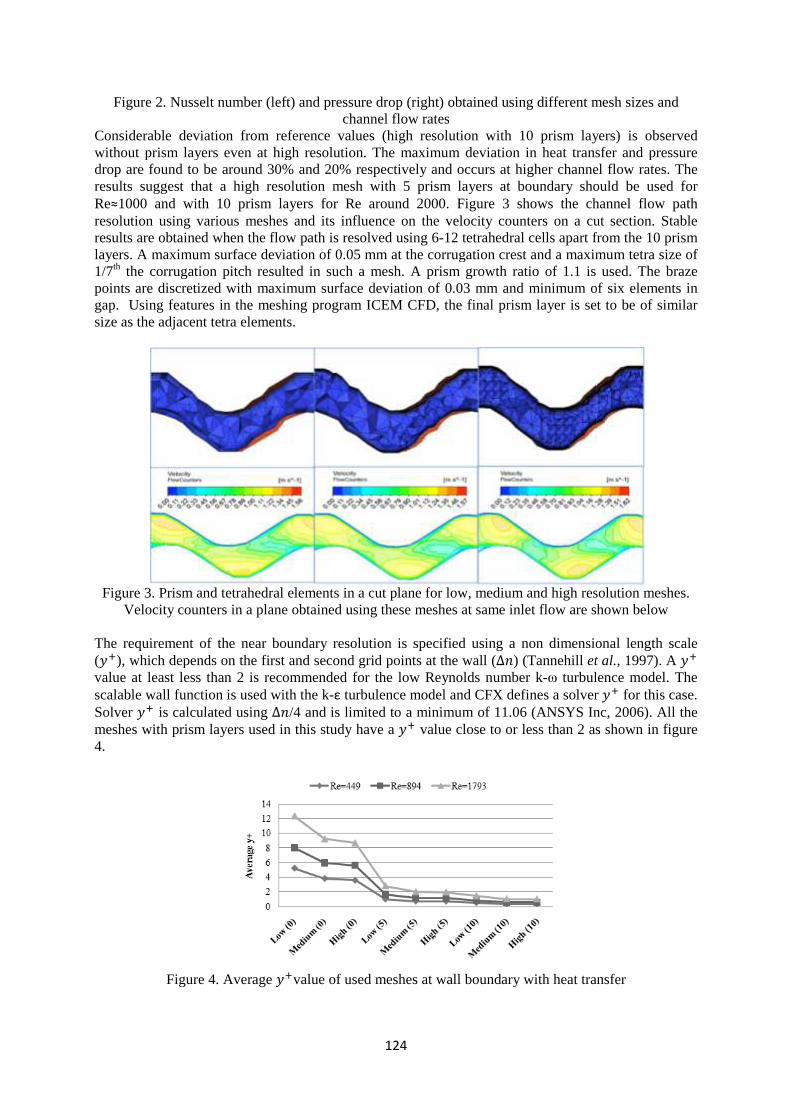
Figure 2. Nusselt number (left) and pressure drop (right) obtained using different mesh sizes and

Considerable deviation from reference values (high resolution with 10 prism layers) is observed without prism layers even at high resolution. The madrop are found to be around 30% and 20% respectively and occurs at higher channel flow rates. The results suggest that a high resolution mesh with 5 prism layers at boundary should be used for Re≈1000 and with resolution using various meshes and its influence on the velocity counters on a cut section. Stable results are obtained when the flow path is resolved using 6layers. A maximum surface deviation of 0.05 mm at the corrugation crest and a maximum tetra size of 1/7th the corrugation pitch resulted in such a mesh. A prism growth ratio of 1.1 is used. The braze points are discretized with maximugap. Using features in the meshing program ICEM CFD, the final prism layer is set to be of similar size as the adjacent tetra elements.

Figure 3. Prism and tetrahedral elements in a cut plaVelocity counters in a plane obtained using these meshes at same inlet flow are shown below

The requirement of the near boundary resolution is specified using a non dimensional length scale (), which depenvalue at least less than 2 is recommended for the low Reynolds number kscalable wall function is used with the kSolver is calculated using meshes with prism layers used in this study have a 4.

Figure 4.

124

Nusselt number (left) and pressure drop (right) obtained using different mesh sizes and channel flow rates

Considerable deviation from reference values (high resolution with 10 prism layers) is observed without prism layers even at high resolution. The madrop are found to be around 30% and 20% respectively and occurs at higher channel flow rates. The results suggest that a high resolution mesh with 5 prism layers at boundary should be used for

1000 and with 10 prism layers for Re around 2000. Figure 3 shows the channel flow path resolution using various meshes and its influence on the velocity counters on a cut section. Stable results are obtained when the flow path is resolved using 6layers. A maximum surface deviation of 0.05 mm at the corrugation crest and a maximum tetra size of

the corrugation pitch resulted in such a mesh. A prism growth ratio of 1.1 is used. The braze points are discretized with maximum surface deviation of 0.03 mm and minimum of six elements in gap. Using features in the meshing program ICEM CFD, the final prism layer is set to be of similar size as the adjacent tetra elements.

Figure 3. Prism and tetrahedral elements in a cut plaVelocity counters in a plane obtained using these meshes at same inlet flow are shown below

The requirement of the near boundary resolution is specified using a non dimensional length scale

), which depends on the first and second grid points at the wall (value at least less than 2 is recommended for the low Reynolds number kscalable wall function is used with the k-ε turbulence model and CFX defines a solver

is calculated using Δ/4 and is limited to a minimum of 11.06 (ANSYS Inc, 2006). All the meshes with prism layers used in this study have a

Figure 4. Average value of used meshes at wall boundary with heat transfer

124

Nusselt number (left) and pressure drop (right) obtained using different mesh sizes and channel flow rates

Considerable deviation from reference values (high resolution with 10 prism layers) is observed without prism layers even at high resolution. The maximum deviation in heat transfer and pressure drop are found to be around 30% and 20% respectively and occurs at higher channel flow rates. The results suggest that a high resolution mesh with 5 prism layers at boundary should be used for

10 prism layers for Re around 2000. Figure 3 shows the channel flow path resolution using various meshes and its influence on the velocity counters on a cut section. Stable results are obtained when the flow path is resolved using 6-12 tetrahedral cells apart from the 10 prism layers. A maximum surface deviation of 0.05 mm at the corrugation crest and a maximum tetra size of

the corrugation pitch resulted in such a mesh. A prism growth ratio of 1.1 is used. The braze m surface deviation of 0.03 mm and minimum of six elements in

gap. Using features in the meshing program ICEM CFD, the final prism layer is set to be of similar

Figure 3. Prism and tetrahedral elements in a cut plane for low, medium and high resolution meshes. Velocity counters in a plane obtained using these meshes at same inlet flow are shown below

The requirement of the near boundary resolution is specified using a non dimensional length scale

ds on the first and second grid points at the wall (Δ) (Tannehill et al.,value at least less than 2 is recommended for the low Reynolds number k-ω turbulence model. The

turbulence model and CFX defines a solver /4 and is limited to a minimum of 11.06 (ANSYS Inc, 2006). All the

meshes with prism layers used in this study have a value close to or less than 2 as shown

value of used meshes at wall boundary with heat transfer

Nusselt number (left) and pressure drop (right) obtained using different mesh sizes and

Considerable deviation from reference values (high resolution with 10 prism layers) is observed ximum deviation in heat transfer and pressure

drop are found to be around 30% and 20% respectively and occurs at higher channel flow rates. The results suggest that a high resolution mesh with 5 prism layers at boundary should be used for

10 prism layers for Re around 2000. Figure 3 shows the channel flow path resolution using various meshes and its influence on the velocity counters on a cut section. Stable

art from the 10 prism layers. A maximum surface deviation of 0.05 mm at the corrugation crest and a maximum tetra size of

the corrugation pitch resulted in such a mesh. A prism growth ratio of 1.1 is used. The braze m surface deviation of 0.03 mm and minimum of six elements in

gap. Using features in the meshing program ICEM CFD, the final prism layer is set to be of similar

ne for low, medium and high resolution meshes.

Velocity counters in a plane obtained using these meshes at same inlet flow are shown below

The requirement of the near boundary resolution is specified using a non dimensional length scale et al., 1997). A

ω turbulence model. The turbulence model and CFX defines a solver for this case.

/4 and is limited to a minimum of 11.06 (ANSYS Inc, 2006). All the value close to or less than 2 as shown in figure

value of used meshes at wall boundary with heat transfer

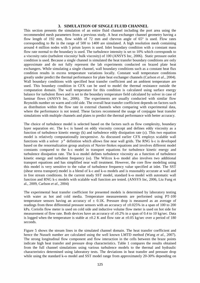
125

3. SIMULATION OF SINGLE FLUID CHANNEL This section presents the simulation of an entire fluid channel including the port area using the recommended mesh parameters from a previous study. A heat exchanger channel geometry having a flow length of 192 mm, flow width of 72 mm and chevron angle of 65° is used. Flow rates corresponding to Re in the range of 500 to 1400 are simulated. A high resolution mesh containing around 4 million nodes with 5 prism layers is used. Inlet boundary condition with a constant mass flow rate normal to the boundary is used. The turbulence intensity is set to 10% which corresponds to a viscosity ratio (turbulent viscosity/ bulk viscosity) of 100 (ANSYS Inc, 2006). Static pressure outlet condition is used. Because a single channel is simulated the heat transfer boundary conditions are only approximate and do not fully represent the lab experiments conducted on brazed plate heat exchangers. While simulating a single channel, wall boundary conditions such as a constant heat flux condition results in excess temperature variations locally. Constant wall temperature conditions greatly under predict the thermal performance for plate heat exchanger channels (Carlson et al., 2004). Wall boundary conditions with specified heat transfer coefficient and an ambient temperature are used. This boundary condition in CFX can be used to model the thermal resistance outside the computation domain. The wall temperature for this condition is calculated using surface energy balance for turbulent flows and is set to the boundary temperature field calculated by solver in case of laminar flows (ANSYS Inc, 2006). The experiments are usually conducted with similar flow Reynolds number on warm and cold side. The overall heat transfer coefficient depends on factors such as distribution within the flow rate in external channels when comparing with experimental data, where the performance is not tested. These factors recommend the usage of conjugate heat transfer simulations with multiple channels and plates to predict the thermal performance with better accuracy. The choice of turbulence model is selected based on the factors such as flow complexity, boundary layer separation etc. The k-ε is based on eddy viscosity concept and defines eddy viscosity as a function of turbulence kinetic energy (k) and turbulence eddy dissipation rate (ε). This two equation model is relatively computationally inexpensive. As discussed earlier CFX employs scalable wall functions with a solver definition which allows fine near wall grids. The RNG k-ε is developed based on the renormalization group analysis of Navier-Stokes equations and involves different model constants compared to the k-ε model in transport equations for turbulence kinetic energy and turbulence dissipation rate. The k-ω model defines turbulence viscosity as a function of turbulence kinetic energy and turbulent frequency (ω). The Wilcox k-ω model also involves two additional transport equations and has simplified near wall treatment. However, the core flow modeling using this model is very sensitive to the value of turbulence frequency value specified at inlet. The SST (shear stress transport) model is a blend of k-ε and k-ω models and is reasonably accurate at wall and in free stream conditions. In the current study SST model, standard k-ω model with automatic wall function and RNG k-ε models with scalable wall function are tested. (ANSYS Inc, 2006, Liu Fung et al., 2009, Carlson et al., 2004) The experimental heat transfer coefficient for presented models is determined by laboratory testing with water as hot and cold media. Temperature measurements are performed using PT-100 temperature sensors having an accuracy of ± 0.1K. Pressure drop is measured as an average of readings from three differential pressure sensors with an accuracy of ±0.025% in a span of 100 to 200 kPa. Coriolis flow meter is used on cold side and inductive volume flow meter is used on hot side for measurement of flow rate. Both devices have an accuracy of ±0.2% in a span of 0.4 to 10 kg/sec. Data is logged when the temperature is stable at ±0.2 K and flow rate at ±0.05 kg/sec over a period of 180 seconds. Figure 5 shows the stream lines in the simulated channel domain. The heat transfer coefficient and hence the Nusselt number are calculated using the well known LMTD method (Wang et al., 2007). The strong longitudinal flow component and flow interaction in the cells between the braze points indicate high heat transfer and pressure drop characteristics. Table 1 compares the results obtained from the full channel simulations using various turbulence models to the thermal and hydraulic characteristics determined using laboratory tests. The deviations in heat transfer and pressure drop while using the standard k-ω model and SST model range from approximately 20-30% depending on

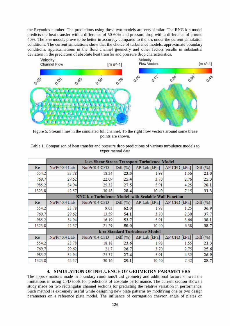
126

the Reynolds number. The predictions using these two models are very similar. The RNG k-ε model predicts the heat transfer with a difference of 50-60% and pressure drop with a difference of around 40%. The k-ω models prove to be better in accuracy compared to the k-ε under the current simulation conditions. The current simulations show that the choice of turbulence models, approximate boundary conditions, approximations in the fluid channel geometry and other factors results in substantial deviation in the prediction of absolute heat transfer and pressure drop characteristics.

Figure 5. Stream lines in the simulated full channel. To the right flow vectors around some braze

points are shown.

Table 1. Comparison of heat transfer and pressure drop predictions of various turbulence models to experimental data

4. SIMULATION OF INFLUENCE OF GEOMETRY PARAMETERS The approximations made in boundary conditions/fluid geometry and additional factors showed the limitations in using CFD tools for predictions of absolute performance. The current section shows a study made on two rectangular channel sections for predicting the relative variation in performance. Such method is extremely useful while designing new plate patterns by modifying one or two design parameters on a reference plate model. The influence of corrugation chevron angle of plates on

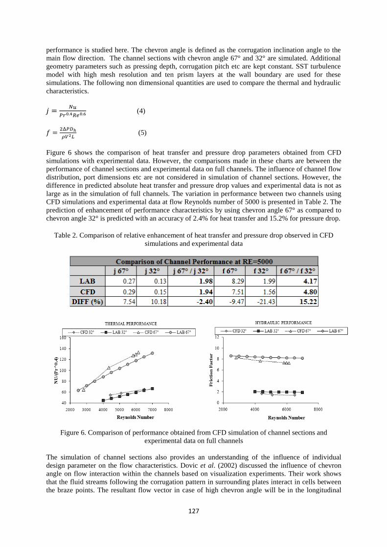
performance is studied here. The chevron angle is defined as the corrugation inclination angle to the main flow direction. The channel sections with chevron angle 67° and 32° are simulated. Additiogeometry parameters such as pressing depth, corrugation pitch etc are kept constant. SST turbulence model with high mesh resolution and ten prism layers at the wall boundary are used for these simulations. The following non dimensional quantities are ucharacteristics.

..

Figure 6 shows the comparison of heat transfer and pressure drop parameters obtained from CFD simulations with experimental data. performance of channel sections and experimental data on full channels. The influence of channel flow distribution, port dimensions etc are not considered in simulation of channel sections. Howedifference in predicted absolute heat transfer and pressure drop values and experimental data is not as large as in the simulation of full channels. The variation in performance between two channels using CFD simulations and experimental data at fprediction of enhancement of performance characteristics by using chevron angle 67° as compared to chevron angle 32° is predicted with an accuracy of 2.4% for heat transfer and 15.2% for pressure dro

Table 2. Comparison of relative enhancement of heat transfer and pressure drop observed in CFD

Figure 6. Comparison of performance obtained from CFD simulation of channel sections and

The simulation of channel sections also provides an understanding of the influence of individual design parameter on the flow characteristicangle on flow interaction within the channels based on visualization experiments. Their work shows that the fluid streams following the corrugation pattern in surrounding plates interact in cells bethe braze points. The resultant flow vector in case of high chevron angle will be in the longitudinal

127

performance is studied here. The chevron angle is defined as the corrugation inclination angle to the main flow direction. The channel sections with chevron angle 67° and 32° are simulated. Additiogeometry parameters such as pressing depth, corrugation pitch etc are kept constant. SST turbulence model with high mesh resolution and ten prism layers at the wall boundary are used for these simulations. The following non dimensional quantities are u

(4)

(5)

Figure 6 shows the comparison of heat transfer and pressure drop parameters obtained from CFD simulations with experimental data. However, the comparisons made in these charts are between the performance of channel sections and experimental data on full channels. The influence of channel flow distribution, port dimensions etc are not considered in simulation of channel sections. Howedifference in predicted absolute heat transfer and pressure drop values and experimental data is not as large as in the simulation of full channels. The variation in performance between two channels using CFD simulations and experimental data at flow Reynolds number of 5000 is presented in Table 2. The prediction of enhancement of performance characteristics by using chevron angle 67° as compared to chevron angle 32° is predicted with an accuracy of 2.4% for heat transfer and 15.2% for pressure dro

Table 2. Comparison of relative enhancement of heat transfer and pressure drop observed in CFD simulations and experimental data

Comparison of performance obtained from CFD simulation of channel sections and experimental data on full channels

The simulation of channel sections also provides an understanding of the influence of individual design parameter on the flow characteristics. Dovic angle on flow interaction within the channels based on visualization experiments. Their work shows that the fluid streams following the corrugation pattern in surrounding plates interact in cells bethe braze points. The resultant flow vector in case of high chevron angle will be in the longitudinal

127

performance is studied here. The chevron angle is defined as the corrugation inclination angle to the main flow direction. The channel sections with chevron angle 67° and 32° are simulated. Additiogeometry parameters such as pressing depth, corrugation pitch etc are kept constant. SST turbulence model with high mesh resolution and ten prism layers at the wall boundary are used for these simulations. The following non dimensional quantities are used to compare the thermal and hydraulic

Figure 6 shows the comparison of heat transfer and pressure drop parameters obtained from CFD However, the comparisons made in these charts are between the

performance of channel sections and experimental data on full channels. The influence of channel flow distribution, port dimensions etc are not considered in simulation of channel sections. Howedifference in predicted absolute heat transfer and pressure drop values and experimental data is not as large as in the simulation of full channels. The variation in performance between two channels using

low Reynolds number of 5000 is presented in Table 2. The prediction of enhancement of performance characteristics by using chevron angle 67° as compared to chevron angle 32° is predicted with an accuracy of 2.4% for heat transfer and 15.2% for pressure dro

Table 2. Comparison of relative enhancement of heat transfer and pressure drop observed in CFD simulations and experimental data

Comparison of performance obtained from CFD simulation of channel sections and experimental data on full channels

The simulation of channel sections also provides an understanding of the influence of individual

s. Dovic et al. (2002) discussed the influence of chevron angle on flow interaction within the channels based on visualization experiments. Their work shows that the fluid streams following the corrugation pattern in surrounding plates interact in cells bethe braze points. The resultant flow vector in case of high chevron angle will be in the longitudinal

performance is studied here. The chevron angle is defined as the corrugation inclination angle to the main flow direction. The channel sections with chevron angle 67° and 32° are simulated. Additional geometry parameters such as pressing depth, corrugation pitch etc are kept constant. SST turbulence model with high mesh resolution and ten prism layers at the wall boundary are used for these

sed to compare the thermal and hydraulic

Figure 6 shows the comparison of heat transfer and pressure drop parameters obtained from CFD However, the comparisons made in these charts are between the

performance of channel sections and experimental data on full channels. The influence of channel flow distribution, port dimensions etc are not considered in simulation of channel sections. However, the difference in predicted absolute heat transfer and pressure drop values and experimental data is not as large as in the simulation of full channels. The variation in performance between two channels using

low Reynolds number of 5000 is presented in Table 2. The prediction of enhancement of performance characteristics by using chevron angle 67° as compared to chevron angle 32° is predicted with an accuracy of 2.4% for heat transfer and 15.2% for pressure drop.

Table 2. Comparison of relative enhancement of heat transfer and pressure drop observed in CFD

Comparison of performance obtained from CFD simulation of channel sections and

The simulation of channel sections also provides an understanding of the influence of individual . (2002) discussed the influence of chevron

angle on flow interaction within the channels based on visualization experiments. Their work shows that the fluid streams following the corrugation pattern in surrounding plates interact in cells between the braze points. The resultant flow vector in case of high chevron angle will be in the longitudinal

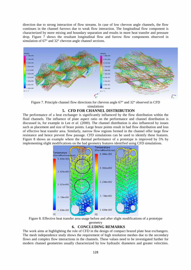
128

direction due to strong interaction of flow streams. In case of low chevron angle channels, the flow continues in the channel furrows due to weak flow interaction. The longitudinal flow component is characterized by more mixing and boundary separation and results in more heat transfer and pressure drop. Figure 7 shows the resultant longitudinal flow and furrow flow components observed in simulation of 67° and 32° chevron angle channel sections.

Figure 7. Principle channel flow directions for chevron angle 67° and 32° observed in CFD

simulations 5. CFD FOR CHANNEL DISTRIBUTION

The performance of a heat exchanger is significantly influenced by the flow distribution within the fluid channels. The influence of plate aspect ratio on the performance and channel distribution is discussed in, for example in Lee et al. (2000). The channel distribution is also influenced by issues such as placement and size of braze points. Large braze points result in bad flow distribution and loss of effective heat transfer area. Similarly, narrow flow regions formed in the channel offer large flow resistance and hence prevent flow passage. CFD simulations can be used to identify these features. Figure 8 shows an example where the thermal performance of a prototype is improved by 5% by implementing slight modifications on the bad geometry features identified using CFD simulations.

Figure 8. Effective heat transfer area usage before and after slight modifications of a prototype

geometry 6. CONCLUDING REMARKS

The work aims at highlighting the role of CFD in the design of compact brazed plate heat exchangers. The mesh independence study shows the requirement of high resolution meshes due to the secondary flows and complex flow interactions in the channels. These values need to be investigated further for modern channel geometries usually characterized by low hydraulic diameters and greater velocities.

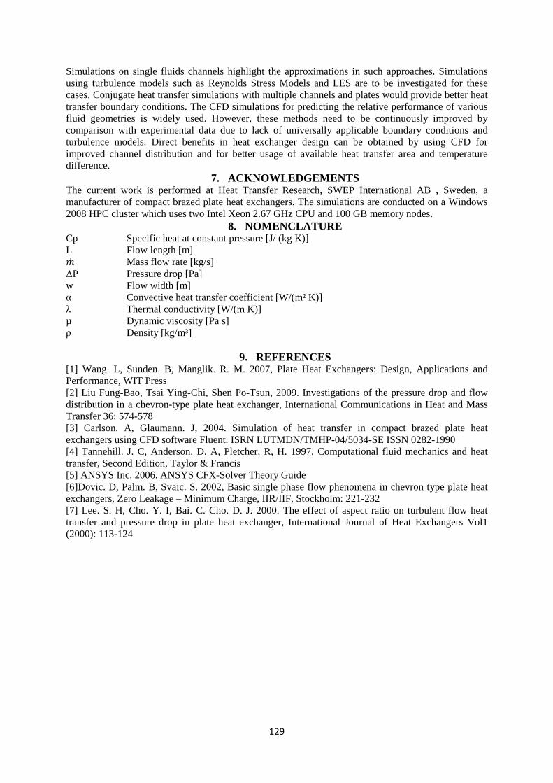
129

Simulations on single fluids channels highlight the approximations in such approaches. Simulations using turbulence models such as Reynolds Stress Models and LES are to be investigated for these cases. Conjugate heat transfer simulations with multiple channels and plates would provide better heat transfer boundary conditions. The CFD simulations for predicting the relative performance of various fluid geometries is widely used. However, these methods need to be continuously improved by comparison with experimental data due to lack of universally applicable boundary conditions and turbulence models. Direct benefits in heat exchanger design can be obtained by using CFD for improved channel distribution and for better usage of available heat transfer area and temperature difference.

7. ACKNOWLEDGEMENTS The current work is performed at Heat Transfer Research, SWEP International AB , Sweden, a manufacturer of compact brazed plate heat exchangers. The simulations are conducted on a Windows 2008 HPC cluster which uses two Intel Xeon 2.67 GHz CPU and 100 GB memory nodes.

8. NOMENCLATURE Cp Specific heat at constant pressure [J/ (kg K)] L Flow length [m] Mass flow rate [kg/s] ∆P Pressure drop [Pa] w Flow width [m] α Convective heat transfer coefficient [W/(m² K)] λ Thermal conductivity [W/(m K)] µ Dynamic viscosity [Pa s] ρ Density [kg/m³]

9. REFERENCES [1] Wang. L, Sunden. B, Manglik. R. M. 2007, Plate Heat Exchangers: Design, Applications and Performance, WIT Press [2] Liu Fung-Bao, Tsai Ying-Chi, Shen Po-Tsun, 2009. Investigations of the pressure drop and flow distribution in a chevron-type plate heat exchanger, International Communications in Heat and Mass Transfer 36: 574-578 [3] Carlson. A, Glaumann. J, 2004. Simulation of heat transfer in compact brazed plate heat exchangers using CFD software Fluent. ISRN LUTMDN/TMHP-04/5034-SE ISSN 0282-1990 [4] Tannehill. J. C, Anderson. D. A, Pletcher, R, H. 1997, Computational fluid mechanics and heat transfer, Second Edition, Taylor & Francis [5] ANSYS Inc. 2006. ANSYS CFX-Solver Theory Guide [6]Dovic. D, Palm. B, Svaic. S. 2002, Basic single phase flow phenomena in chevron type plate heat exchangers, Zero Leakage – Minimum Charge, IIR/IIF, Stockholm: 221-232 [7] Lee. S. H, Cho. Y. I, Bai. C. Cho. D. J. 2000. The effect of aspect ratio on turbulent flow heat transfer and pressure drop in plate heat exchanger, International Journal of Heat Exchangers Vol1 (2000): 113-124

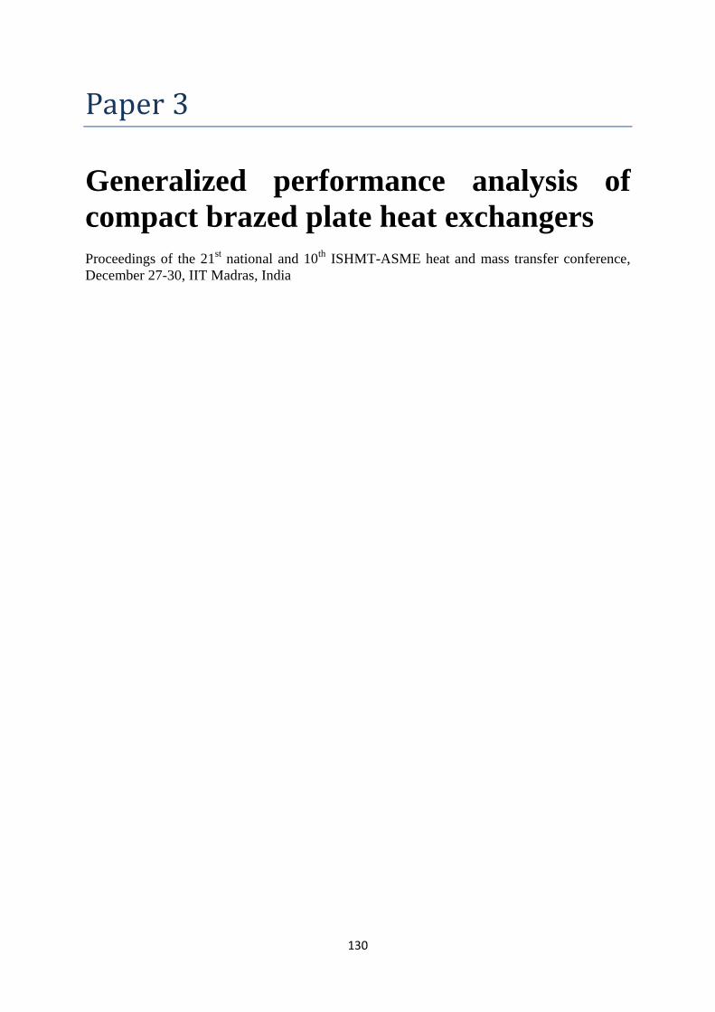
130

Paper 3

Generalized performance analysis of compact brazed plate heat exchangers Proceedings of the 21st national and 10th ISHMT-ASME heat and mass transfer conference, December 27-30, IIT Madras, India

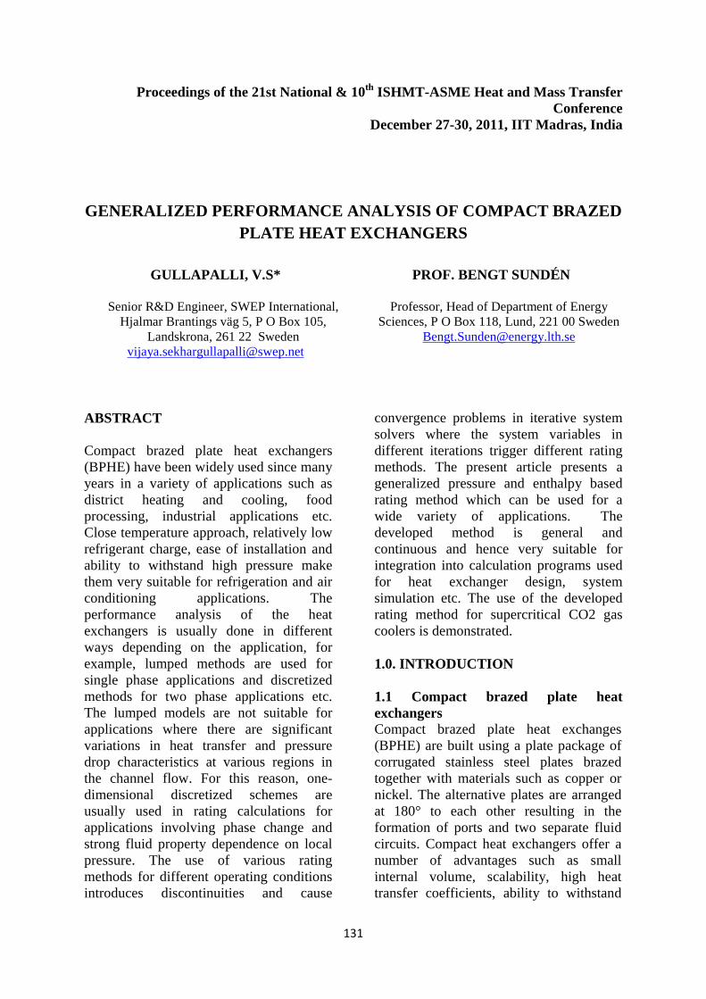
131

Proceedings of the 21st National & 10th ISHMT-ASME Heat and Mass Transfer Conference

December 27-30, 2011, IIT Madras, India

GENERALIZED PERFORMANCE ANALYSIS OF COMPACT BRAZED PLATE HEAT EXCHANGERS

GULLAPALLI, V.S*

Senior R&D Engineer, SWEP International, Hjalmar Brantings väg 5, P O Box 105,

Landskrona, 261 22 Sweden vijaya.sekhargullapalli@swep.net

PROF. BENGT SUNDÉN

Professor, Head of Department of Energy Sciences, P O Box 118, Lund, 221 00 Sweden

Bengt.Sunden@energy.lth.se

ABSTRACT Compact brazed plate heat exchangers (BPHE) have been widely used since many years in a variety of applications such as district heating and cooling, food processing, industrial applications etc. Close temperature approach, relatively low refrigerant charge, ease of installation and ability to withstand high pressure make them very suitable for refrigeration and air conditioning applications. The performance analysis of the heat exchangers is usually done in different ways depending on the application, for example, lumped methods are used for single phase applications and discretized methods for two phase applications etc. The lumped models are not suitable for applications where there are significant variations in heat transfer and pressure drop characteristics at various regions in the channel flow. For this reason, one-dimensional discretized schemes are usually used in rating calculations for applications involving phase change and strong fluid property dependence on local pressure. The use of various rating methods for different operating conditions introduces discontinuities and cause

convergence problems in iterative system solvers where the system variables in different iterations trigger different rating methods. The present article presents a generalized pressure and enthalpy based rating method which can be used for a wide variety of applications. The developed method is general and continuous and hence very suitable for integration into calculation programs used for heat exchanger design, system simulation etc. The use of the developed rating method for supercritical CO2 gas coolers is demonstrated. 1.0. INTRODUCTION

1.1 Compact brazed plate heat exchangers Compact brazed plate heat exchanges (BPHE) are built using a plate package of corrugated stainless steel plates brazed together with materials such as copper or nickel. The alternative plates are arranged at 180° to each other resulting in the formation of ports and two separate fluid circuits. Compact heat exchangers offer a number of advantages such as small internal volume, scalability, high heat transfer coefficients, ability to withstand

132

high operating pressures etc. Further information on the construction, materials and applications of BPHE can be found, for example, in (Wang et al., 2007) 1.2 Heat exchangers sizing and rating The rating of heat exchangers involves calculation of the suitability of a heat exchanger for a given thermal and hydraulic requirement. In the LMTD method, the rating calculations involve calculation of area required for the specified heat transfer duty, which depends on factors such as flow conditions, fluid channel and plate characteristics and local temperature profiles. (Wang et al. 2007)

( ).required LMTDA Q U T= ∆ (1)

In lumped models, the logarithmic mean temperature difference is calculated using end temperatures and the overall heat transfer coefficient is determined at a mean reference temperature. The suitability of the heat exchanger is then stated using parameters such as over surface ().

.100available required

available

A AOS

A

−= (2)

The total pressure drop in the brazed plate heat exchanger includes contribution of pressure drop in connections, port manifolds, and distribution devices and fluids channels. The pressure drop in the fluid channels influences the heat transfer area requirement in case of applications where there is strong dependence of fluid properties on local pressure. The sizing of the plate heat exchangers involves iterative rating calculations to determine the number of plates, flow arrangement and passes for specified heat transfer and pressure drop requirement. The lumped models are not suitable for applications where there are significant variations in heat transfer and pressure drop characteristics at various regions in the channel flow. For this reason, one-

dimensional discretized schemes are usually used in rating calculations for applications involving phase change and strong fluid property dependence on local pressure (Wang et al., 1999). Other performance calculation methods involving 2-D flow paths are proposed for better modeling of flow maldistribution, multiple pass configurations etc. However, these methods are computationally expensive and have convergence problems at low flow rates and close local temperature approaches (Gullapalli 2005). 2.0 GENERALIZED RATING METHOD Rating calculations are widely used in thermal and hydraulic system simulation programs. Iterative algorithms in the system simulation programs require continuous and fast calculation of heat exchanger performance. The use of various rating methods for different operating conditions introduces discontinuities and cause convergence problems in system solvers where the variables in different iterations trigger different rating methods. Scalability is also a desired characteristic of rating methods. It is generally not possible to calibrate heat transfer and pressure drop correlations in a wide range of operating conditions. The rating method is expected to handle additional influences by parameters such a local temperature difference and sudden variation of fluid properties at certain operating conditions. The current study involves developing a continuous and robust plate heat exchanger rating method which can be applied for a wide range of operating conditions. 2.1 Calculation Procedure The generalized rating method involves one dimensional discretization of the plate heat exchanger into cells of equal heat load as shown in Figure 1. Each cell is characterized by two fluids elements representing two sides of a heat exchanger and a wall element representing the local

plate. The fluid elements are extended between two fluid nodes which repthe local enthalpy and pressure. Fluid elements are used to determine local heat transfer coefficients and pressure drops. The fluid properties in a fluid element are determined at the mean pressure and enthalpy. The rating calculation involves determining the area required at each cell iteratively by adjusting the local temperature and pressure profiles. The convergence of this iterative rating method is governed by the convergence of wall node temperatures.

Figure 1: Schematic of the scheme used in generalized rating method for counter current flow arrangement. The steps involved in this generalized rating method are listed below: Step 1: The supplied inlet pressure and end temperatures for a BPHE rating calculation are applied as pressureenthalpy boundary conditions at the end nodes. The enthalpy at the outlet is determined using a trial value for pressure drop. Step 2: The discretized cells are assigned a local heat load (Q

133

plate. The fluid elements are extended between two fluid nodes which represent the local enthalpy and pressure. Fluid elements are used to determine local heat transfer coefficients and pressure drops. The fluid properties in a fluid element are determined at the mean pressure and enthalpy. The rating calculation involves

ermining the area required at each cell iteratively by adjusting the local temperature and pressure profiles. The convergence of this iterative rating method is governed by the convergence of wall node temperatures.

Figure 1: Schematic of the discretization scheme used in generalized rating method for counter current flow arrangement.

The steps involved in this generalized rating method are listed below:

: The supplied inlet pressure and end temperatures for a BPHE rating

e applied as pressure-enthalpy boundary conditions at the end nodes. The enthalpy at the outlet is determined using a trial value for pressure

: The discretized cells are assigned a Qn) which is determined as

133

nQ Q N=

where ‘N’ represents the number of discretized sections. The fluid elements connected to each of these cells are assigned the mass flow rate corresponding to specified or calculated flow rates on their side. Trail values are set for pressure drop in fluid elements and for temperature in wall nodes during the first iteration. Step 3: Using the energy balance, the enthalpy at various nodes is determined. The heat transfer coefficient and pressure drop in each element are calculated. The choice of heat transfer and pressure drop correlations is based on the mean pressure, mean enthalpy and the wall temperature. Further discretization of the cell is required in case of phase change in the fluid elements of a cell. This is done by splitting the cell where the saturation temperature is crossed. Fluid properties at the wall are determined at wall temperature. The area required for each cell is determined using the following equations.

1

1 2

1 1n wall

E E

U Rα α

−

= + +

(, ,.required n n n LMTD nA Q U T= ∆ Step 4: The wall temperatures in each cell are then determined using energy balance as follows

( ),1 1 1 21

nwall E E E

E

UT T T T

α= − −

( ),2 2 2 12

nwall E E E

E

UT T T T

α= − −

Step 5: The total area required for the specified rating case is then calculated as sum of the area required by each cell. The pressure drop calculation in each cell requires the flow length. This is set to the product of total flow length and the ratio of area required in each cell to the total area required. The outlet enthalpy is recalculated using the updated pressure

(3)

‘N’ represents the number of discretized sections. The fluid elements connected to each of these cells are assigned the mass flow rate corresponding to specified or calculated flow rates on their side. Trail values are set for pressure

nts and for temperature in wall nodes during the first iteration.

: Using the energy balance, the enthalpy at various nodes is determined. The heat transfer coefficient and pressure drop in each element are calculated. The

and pressure drop correlations is based on the mean pressure, mean enthalpy and the wall temperature. Further discretization of the cell is required in case of phase change in the fluid elements of a cell. This is done by splitting

ation temperature is crossed. Fluid properties at the wall are determined at wall temperature. The area required for each cell is determined using

(4)

)required n n n LMTD n (5)

The wall temperatures in each cell are then determined using energy balance

(6)

),2 2 2 1 (7)

The total area required for the specified rating case is then calculated as sum of the area required by each cell. The pressure drop calculation in each cell requires the flow length. This is set to the product of total flow length and the ratio of

equired in each cell to the total area required. The outlet enthalpy is recalculated using the updated pressure

134

drop on each side. All the calculated rating parameters such as flow rates that are initially set based on the energy balance are recalculated using the updated end enthalpies. The wall temperature residue is calculated as a root mean square variation of all wall node temperatures during the iterations. The calculation continues until the wall temperature residue reaches a specified minimum value. 2.3 Heat transfer correlations Thermal and hydraulic characteristics of plate heat exchangers depend on a number of geometry parameters such as chevron angle, pressing depth, corrugation pitch, plate aspect ratio, port dimensions etc. A number of general correlations for heat transfer and pressure drop published for single phase applications are summarized, for example in (Wang et al., 2007). The lack of generality in the definition of standard geometry parameters, rapid improvements in plate design for better distribution etc does not support the development of generalized correlations. Empirical constants such as performance enhancement and suppression factors are evaluated for each product based on experimental data. The single phase heat transfer correlation due to Bogaert and Bolcs is generally suitable for single phase applications (Wang et al., 2007)

21 Re PrC yNu C ϕ= (8)

The empirical constants 1C and 2C are

evaluated from laboratory data. The Prandtl number exponent ‘y’ is defined as a function of Prandtl number itself. The correction factor ϕ accounts for the variation of dynamic viscosity in the core of the fluid channel and at the wall. Heat transfer coefficient during evaporation is defined by equations that have been suggested by Chen (1996). The local heat transfer coefficient is a weighted average of the contributions of convective

and nucleate boiling. Convective boiling is determined from single phase heat transfer characteristics and nucleate boiling coefficient is dependent on local temperature difference, wall temperature etc. Heat transfer coefficient during condensation is calculated as a root mean square average value of contributions from the gravity and shear controlled regime as suggested by Thonon (1995) 3.0. FINITE GRID INTERPOLATION METHOD FOR FLUID PROPERTIES Saturated and bulk refrigerant properties are necessary to calculate the local heat transfer coefficients and friction factors in BPHE rating calculations. Thermodynamic properties such as pressure, enthalpy, temperature, density, specific heat and transport properties such as thermal conductivity, dynamic viscosity are usually obtained from standard databases such as NIST REFPROP. The direct use of REFPROP can be unsuitable in heat exchanger selection tools due to the large computation delay caused by (a) the iterative methods used by REFPROP for solving the equations of state, particularly for refrigerant mixtures and (b) direct reference limitations of other programming languages with REFPROP libraries. Polynomial fitting and other non linear regression methods are often used for modeling individual fluid properties but it is often not possible to use a single model for the entire pressure-enthalpy domain. Hence separate models are required in various regions. Such models are faster and simple to use in calculation software, but they introduce discontinuities at the region boundaries and can cause problems in iterative calculations. Heat exchanger selection involves iterative use of rating calculations which in turn make numerous calls to the fluid property libraries. For robust rating calculations it is required that the fluid properties obtained are accurate, fast and continuous. A

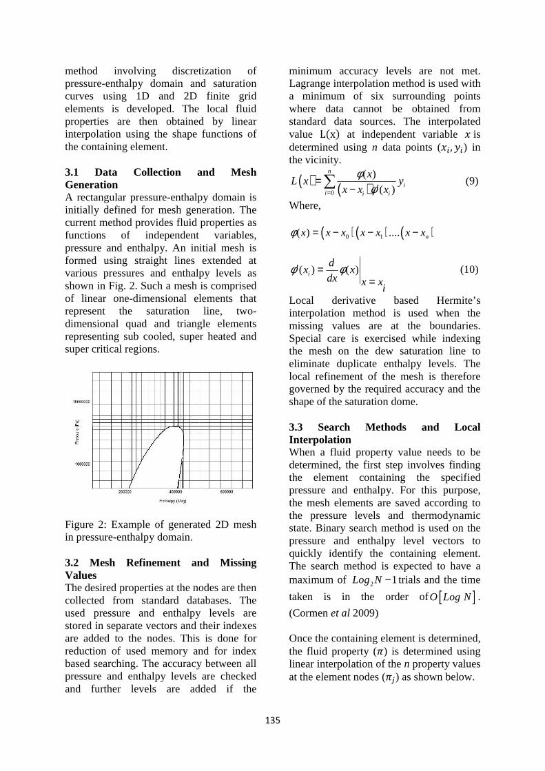
135

method involving discretization of pressure-enthalpy domain and saturation curves using 1D and 2D finite grid elements is developed. The local fluid properties are then obtained by linear interpolation using the shape functions of the containing element. 3.1 Data Collection and Mesh Generation A rectangular pressure-enthalpy domain is initially defined for mesh generation. The current method provides fluid properties as functions of independent variables, pressure and enthalpy. An initial mesh is formed using straight lines extended at various pressures and enthalpy levels as shown in Fig. 2. Such a mesh is comprised of linear one-dimensional elements that represent the saturation line, two-dimensional quad and triangle elements representing sub cooled, super heated and super critical regions.

Figure 2: Example of generated 2D mesh in pressure-enthalpy domain.

3.2 Mesh Refinement and Missing Values The desired properties at the nodes are then collected from standard databases. The used pressure and enthalpy levels are stored in separate vectors and their indexes are added to the nodes. This is done for reduction of used memory and for index based searching. The accuracy between all pressure and enthalpy levels are checked and further levels are added if the

minimum accuracy levels are not met. Lagrange interpolation method is used with a minimum of six surrounding points where data cannot be obtained from standard data sources. The interpolated value Lx at independent variable is determined using n data points ( ,) in the vicinity.

( ) ( )0

( )

( )

n

ii i i

xL x y

x x x

φφ=

=′−∑

(9)

Where,

( )( ) ( )0 1( ) .... nx x x x x x xφ = − − −

( ) ( )i

dx x

dx x xi

φ φ′ ==

(10)

Local derivative based Hermite’s interpolation method is used when the missing values are at the boundaries. Special care is exercised while indexing the mesh on the dew saturation line to eliminate duplicate enthalpy levels. The local refinement of the mesh is therefore governed by the required accuracy and the shape of the saturation dome. 3.3 Search Methods and Local Interpolation When a fluid property value needs to be determined, the first step involves finding the element containing the specified pressure and enthalpy. For this purpose, the mesh elements are saved according to the pressure levels and thermodynamic state. Binary search method is used on the pressure and enthalpy level vectors to quickly identify the containing element. The search method is expected to have a maximum of 2 1Log N− trials and the time

taken is in the order of[ ]O Log N .

(Cormen et al 2009) Once the containing element is determined, the fluid property () is determined using linear interpolation of the n property values at the element nodes () as shown below.

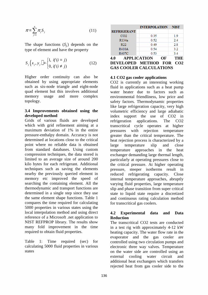
136

1

n

j jj

Sπ π=

=∑ (11)

The shape functions () depends on the type of element and have the property

( ) 1, ( ),

0, ( )j j j

if i jS x y

if i j

== ≠

(12)

Higher order continuity can also be obtained by using appropriate elements such as six-node triangle and eight-node quad element but this involves additional memory usage and more complex topology. 3.4 Improvements obtained using the developed method Grids of various fluids are developed which with grid refinement aiming at a maximum deviation of 1% in the entire pressure-enthalpy domain. Accuracy is not determined at locations close to the critical point where no reliable data is obtained from standard databases. Using custom compression techniques, the data stored is limited to an average size of around 200 kilo bytes for each refrigerant. Additional techniques such as saving the elements nearby the previously queried element in memory etc improved the speed of searching the containing element. All the thermodynamic and transport functions are determined in a single step since they use the same element shape functions. Table 1 compares the time required for calculating 5000 properties in various states using the local interpolation method and using direct reference of a Microsoft .net application to NIST REFPROP library. The results show many fold improvement in the time required to obtain fluid properties. Table 1: Time required (sec) for calculating 5000 fluid properties in various states

4.0 APPLICATION OF THE DEVELOPED METHOD FOR CO2 GAS COOLER CALCULATIONS 4.1 CO2 gas cooler applications CO2 is currently an interesting working fluid in applications such as a heat pump water heater due to factors such as environmental friendliness, low price and safety factors. Thermodynamic properties like large refrigeration capacity, very high volumetric efficiency and large adiabatic index support the use of CO2 in refrigeration applications. The CO2 transcritical cycle operates at higher pressures with rejection temperature greater than the critical temperature. The heat rejection process is characterized by a large temperature slip and close temperature approaches in the heat exchanger demanding large thermal length, particularly at operating pressures close to the critical pressure. At higher operating pressure, steeper isotherms result in reduced refrigerating capacity. Close internal temperature approaches, abruptly varying fluid properties, large temperature slip and phase transition from super critical state to liquid state require a discretized and continuous rating calculation method for transcritical gas coolers. 4.2 Experimental data and Data Reduction The transcritical CO2 tests are conducted in a test rig with approximately 4-12 kW heating capacity. The water flow rate in the evaporator and the gas cooler are controlled using two circulation pumps and electronic three way valves. Temperature on the water side are controlled using an external cooling water circuit and additional heat exchangers which transfers rejected heat from gas cooler side to the

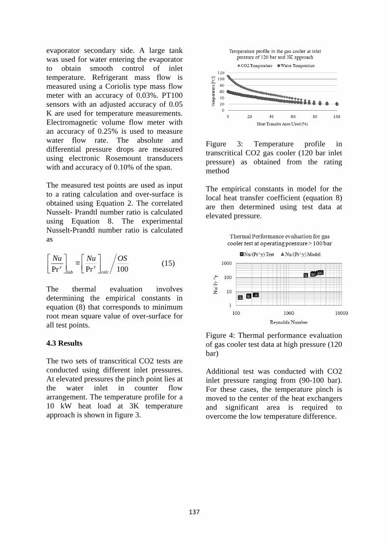
evaporator secondary side. A large tank was used for water entering the evaporator to obtain smooth control of inlet temperature. Refrigerant mass flow is measured using a Coriolis type mass flow meter with an accuracy of 0.03%. PT100 sensors with an adjusted accuracy of 0.05 K are used for temperature Electromagnetic volume flow meter with an accuracy of 0.25% is used to measure water flow rate. The absolute and differential pressure drops are measured using electronic Rosemount transducers with and accuracy of 0.10% of the span. The measured test points are used as input to a rating calculation and overobtained using Equation 2. The correlated Nusselt- Prandtl number ratio is calculated using Equation 8. The experimental Nusselt-Prandtl number ratio is calculated as

Pr 100Pr yylab

Nu Nu OS = The thermal evaluation involves determining the empirical constants in equation (8) that corresponds to minimum root mean square value of overall test points. 4.3 Results The two sets of transcritical CO2 tests are conducted using different inlet pressures. At elevated pressures the pinch point lies at the water inlet in counter flow arrangement. The temperature profile for a 10 kW heat load at 3K temperature approach is shown in figure 3.

137

evaporator secondary side. A large tank for water entering the evaporator

to obtain smooth control of inlet temperature. Refrigerant mass flow is measured using a Coriolis type mass flow meter with an accuracy of 0.03%. PT100 sensors with an adjusted accuracy of 0.05 K are used for temperature measurements. Electromagnetic volume flow meter with an accuracy of 0.25% is used to measure water flow rate. The absolute and differential pressure drops are measured using electronic Rosemount transducers with and accuracy of 0.10% of the span.

ured test points are used as input to a rating calculation and over-surface is obtained using Equation 2. The correlated

Prandtl number ratio is calculated using Equation 8. The experimental

Prandtl number ratio is calculated

Pr 100ycalc

Nu OS

(15)

The thermal evaluation involves determining the empirical constants in equation (8) that corresponds to minimum root mean square value of over-surface for

The two sets of transcritical CO2 tests are conducted using different inlet pressures. At elevated pressures the pinch point lies at the water inlet in counter flow arrangement. The temperature profile for a 10 kW heat load at 3K temperature

own in figure 3.

137

Figure 3: Temperature profile in transcritical CO2 gas cooler (120 bar inlet pressure) as obtained from the rating method The empirical constants in model for the local heat transfer coefficient (equation 8) are then determined usingelevated pressure.

Figure 4: Thermal performance evaluation of gas cooler test data at high pressure (120 bar) Additional test was conducted with CO2 inlet pressure ranging from (90For these cases, the temperature pinch is moved to the center of the heat exchangers and significant area is required to overcome the low temperature difference.

Figure 3: Temperature profile in transcritical CO2 gas cooler (120 bar inlet pressure) as obtained from the rating

The empirical constants in model for the local heat transfer coefficient (equation 8) are then determined using test data at

Figure 4: Thermal performance evaluation of gas cooler test data at high pressure (120

Additional test was conducted with CO2 inlet pressure ranging from (90-100 bar). For these cases, the temperature pinch is

d to the center of the heat exchangers and significant area is required to overcome the low temperature difference.

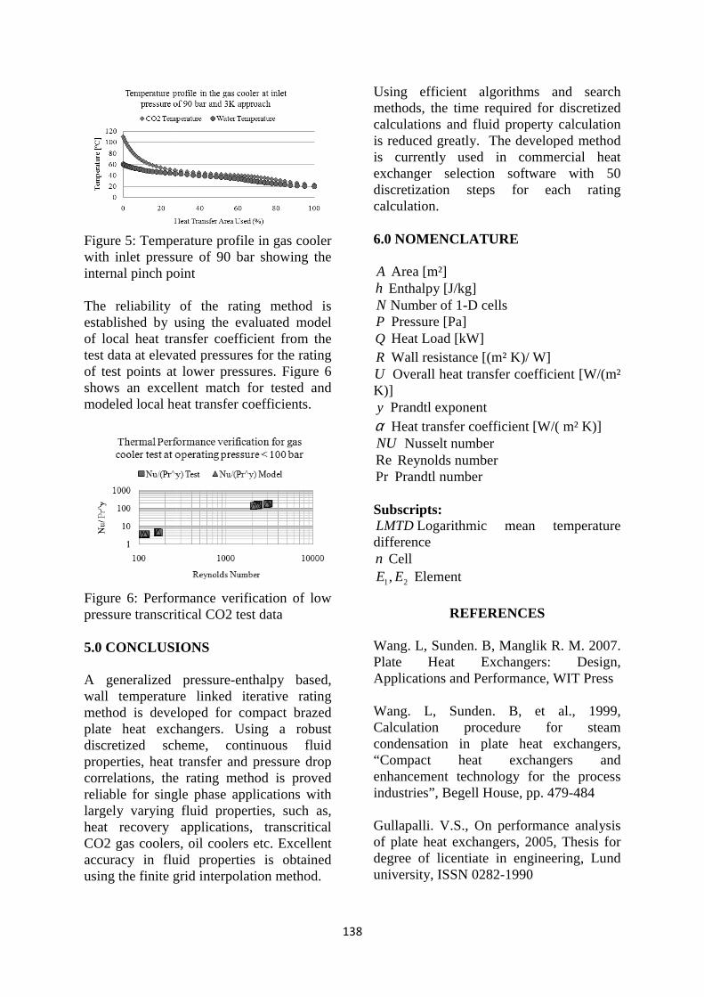
Figure 5: Temperature profile in gas cooler with inlet pressure of 90 bar showing the internal pinch point The reliability of the ratinestablished by using the evaluated model of local heat transfer coefficient from the test data at elevated pressures for the rating of test points at lower pressures. Figure 6 shows an excellent match for tested and modeled local heat transfer

Figure 6: Performance verification of low pressure transcritical CO2 test data 5.0 CONCLUSIONS A generalized pressurewall temperature linked iterative rating method is developed for compact brazed plate heat exchangers.discretized scheme, continuous fluid properties, heat transfer and pressure drop correlations, the rating method is proved reliable for single phase applications with largely varying fluid properties, such as, heat recovery applications, trCO2 gas coolers, oil coolers etc. Excellent accuracy in fluid properties is obtained using the finite grid interpolation method.

138

Figure 5: Temperature profile in gas cooler with inlet pressure of 90 bar showing the internal pinch point

The reliability of the rating method is established by using the evaluated model of local heat transfer coefficient from the test data at elevated pressures for the rating of test points at lower pressures. Figure 6 shows an excellent match for tested and modeled local heat transfer coefficients.

Figure 6: Performance verification of low pressure transcritical CO2 test data

5.0 CONCLUSIONS

A generalized pressure-enthalpy based, wall temperature linked iterative rating method is developed for compact brazed plate heat exchangers. Using a robust discretized scheme, continuous fluid properties, heat transfer and pressure drop correlations, the rating method is proved reliable for single phase applications with largely varying fluid properties, such as, heat recovery applications, transcritical CO2 gas coolers, oil coolers etc. Excellent accuracy in fluid properties is obtained using the finite grid interpolation method.

138

Using efficient algorithms and search methods, the time required for discretized calculations and fluid property cais reduced greatly. The developed method is currently used in commercial heat exchanger selection software with 50 discretization steps for each rating calculation. 6.0 NOMENCLATURE A Area [m²] h Enthalpy [J/kg] N Number of 1-D cells P Pressure [Pa] Q Heat Load [kW] R Wall resistance [(m² K)/ W]U Overall heat transfer coefficient [W/(m² K)] y Prandtl exponent α Heat transfer coefficient [W/( m² K)] NU Nusselt number Re Reynolds number Pr Prandtl number Subscripts: LMTD Logarithmic mean temperature difference n Cell

1 2,E E Element

REFERENCES

Wang. L, Sunden. B, Manglik R. M. 2007. Plate Heat Exchangers: Design, Applications and Performance, WIT Press Wang. L, Sunden. B, et al., 1999, Calculation procedure for steam condensation in plate heat exchangers, “Compact heat exchangers and enhancement technology for the process industries”, Begell House, pp. 479 Gullapalli. V.S., On performance analysis of plate heat exchangers, 2005, Thesis for degree of licentiate in engineering, Lund university, ISSN 0282-1990

Using efficient algorithms and search methods, the time required for discretized calculations and fluid property calculation is reduced greatly. The developed method is currently used in commercial heat exchanger selection software with 50 discretization steps for each rating

Wall resistance [(m² K)/ W] Overall heat transfer coefficient [W/(m²

Heat transfer coefficient [W/( m² K)]

Logarithmic mean temperature

REFERENCES

L, Sunden. B, Manglik R. M. 2007. Plate Heat Exchangers: Design, Applications and Performance, WIT Press

L, Sunden. B, et al., 1999, Calculation procedure for steam condensation in plate heat exchangers, “Compact heat exchangers and enhancement technology for the process industries”, Begell House, pp. 479-484

Gullapalli. V.S., On performance analysis te heat exchangers, 2005, Thesis for

degree of licentiate in engineering, Lund 1990

139

Chen J. C, (1996). A correlation for boiling heat transfer to saturated fluids in convective flow, Industrial and engineering chemistry process design and development, 1996, 5(3), pp 322-329 Thonon. B., Chopard. F. 1995. Condensation in plate heat exchangers:

assessment of a general design method. Eurotherm seminar: Heat transfer in condensation, Paris, Elsevier, pp 10-18 Cormen. T. H. et al., Introduction to Algorithms, 2009, Massachusetts Institute of Technology.

140

Paper 4

Condensation and evaporation in compact brazed plate heat exchangers: Generalized rating method Proceedings of the 21st national and 10th ISHMT-ASME heat and mass transfer conference, December 27-30, IIT Madras, India

141

Proceedings of the 21st National & 10th ISHMT-ASME Heat and Mass Transfer Conference

December 27-30, 2011, IIT Madras, India

CONDENSATION AND EVAPORATION IN COMPACT BRAZED PLATE HEAT EXCHANGERS: GENERALIZED RATING METHOD

GULLAPALLI, V.S*

Senior R&D Engineer, SWEP International, Hjalmar Brantings väg 5, P O Box 105,

Landskrona, 261 22 Sweden vijaya.sekhargullapalli@swep.net

PROF. BENGT SUNDÉN

Professor, Head of Department of Energy Sciences, P O Box 118, Lund, 221 00 Sweden

Bengt.Sunden@energy.lth.se

ABSTRACT Performance analysis and selection of plate heat exchangers for specified duty involves iterative use of rating calculations. The rating method determines the suitability of a heat exchanger for a given thermal duty and pressure drop requirement. A generalized and continuous discretized rating method is described in detail in this paper. Standard and continuous forms of heat transfer correlations that are used with this method are presented. The developed method together with experimental data is used to evaluate empirical constants in heat transfer correlations. 1.0 INTRODUCTION Compact brazed plate heat exchangers (BPHE) are increasingly used for condenser and evaporator applications in process and refrigeration industries. These heat exchangers are associated with benefits such as high thermal performance, refrigerant charge reduction, close temperature approaches and ability to handle higher operating pressures. The working principal, construction and materials used in these units are described in Wang et. al (2007). The thermal and hydraulic performance of BPHE is

dependent on a number of parameters which include the geometric features of the plate, fluid properties, flow rates and thermodynamic parameters. The distribution of heat transfer media in the heat exchanger port manifolds and within the channels also has significant influence on the performance. Various correlations are available in literature for local heat transfer coefficient and pressure drop during condensation and evaporation in plate heat exchangers. These correlations are used with a wide range of design algorithms and definitions of non dimensional numbers. The use of multiple correlations introduces discontinuities in the rating calculations which in turn pose a problem for iterative programs used for system level simulation, heat exchanger selection etc. The lack of generality in the model for various phase change applications such as evaporators, condensers and cascaded heat exchangers limits the extendibility of the model to various operating conditions. A continuous and general wall temperature linked discretized rating method for condensation and evaporation in plate heat exchangers is presented in this paper. The pressure enthalpy based rating method is general for all applications and employs

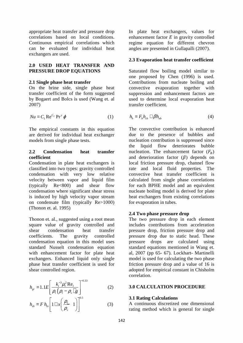
142

appropriate heat transfer and pressure drop correlations based on local conditions. Continuous empirical correlations which can be evaluated for individual heat exchangers are used. 2.0 USED HEAT TRANSFER AND PRESSURE DROP EQUATIONS 2.1 Single phase heat transfer On the brine side, single phase heat transfer coefficient of the form suggested by Bogaert and Bolcs is used (Wang et. al 2007)

21 Re PrC yNu C ϕ= (1)

The empirical constants in this equation are derived for individual heat exchanger models from single phase tests. 2.2 Condensation heat transfer coefficient Condensation in plate heat exchangers is classified into two types: gravity controlled condensation with very low relative velocity between vapor and liquid film (typically Re<800) and shear flow condensation where significant shear stress is induced by high velocity vapor stream on condensate film (typically Re>1000) (Thonon et. al. 1995) Thonon et. al., suggested using a root mean square value of gravity controlled and shear condensation heat transfer coefficients. The gravity controlled condensation equation in this model uses standard Nusselt condensation equation with enhancement factor for plate heat exchangers. Enhanced liquid only single phase heat transfer coefficient is used for shear controlled region.

( )

0.333 2Re

1.1 l l lgr

l l v

kh E

g

µρ ρ ρ

−−

= − (2)

0.5

1 1lsh lo

v

h F h xρρ

= + −

(3)

In plate heat exchangers, values for enhancement factor in gravity controlled regime equation for different chevron angles are presented in Gullapalli (2007). 2.3 Evaporation heat transfer coefficient Saturated flow boiling model similar to one proposed by Chen (1996) is used. Contributions from nucleate boiling and convective evaporation together with suppression and enhancement factors are used to determine local evaporation heat transfer coefficient.

b b cb nbh F h hβ= + (4)

The convective contribution is enhanced due to the presence of bubbles and nucleation contribution is suppressed since the liquid flow deteriorates bubble nucleation. The enhancement factor () and deterioration factor () depends on local friction pressure drop, channel flow rate and local fluid properties. The convective heat transfer coefficient is calculated from single phase correlations for each BPHE model and an equivalent nucleate boiling model is derived for plate heat exchangers from existing correlations for evaporation in tubes. 2.4 Two phase pressure drop The two pressure drop in each element includes contributions from acceleration pressure drop, friction pressure drop and pressure drop due to static head. These pressure drops are calculated using standard equations mentioned in Wang et. al, 2007 (pp 65- 67). Lockhart- Martinelli model is used for calculating the two phase friction pressure drop and a value of 16 is adopted for empirical constant in Chisholm correlation. 3.0 CALCULATION PROCEDURE 3.1 Rating Calculations A continuous discretized one dimensional rating method which is general for single

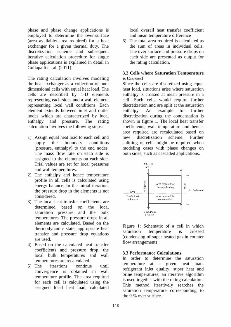
phase and phase change applications is employed to determine the over(area available/ area required) for a heat exchanger for a given thermal duty. The discretization scheme and subsequent iterative calculation procedure for single phase applications is explained in detail in Gullapalli et. al, (2011). The rating calculation involves modeling the heat exchanger as a collection of onedimensional cells with equacells are described by 1representing each sides and a wall element representing local wall conditions. Each element extends between inlet and outlet nodes which are characterized by local enthalpy and pressure. The rating calculation involves the following steps: 1) Assign equal heat load to each cell and

apply the boundary conditions (pressure, enthalpy) to the end nodes. The mass flow rate on each side is assigned to the elements on each side. Trial values are set for local presand wall temperatures.

2) The enthalpy and hence temperature profile in all cells is calculated using energy balance. In the initial iteration, the pressure drop in the elements is not considered.

3) The local heat transfer coefficients are determined basesaturation pressure and the bulk temperatures. The pressure drops in all elements are calculated. Based on the thermodynamic state, appropriate heat transfer and pressure drop equations are used.

4) Based on the calculated heat transfer coefficients and pressure drop, the local bulk temperatures and wall temperatures are recalculated.

5) The iterations continue until convergence is obtained in wall temperature profile. The area required for each cell is calculated using the assigned local heat load, calculated

143

phase and phase change applications is employed to determine the over-surface (area available/ area required) for a heat exchanger for a given thermal duty. The

ation scheme and subsequent iterative calculation procedure for single phase applications is explained in detail in Gullapalli et. al, (2011).

The rating calculation involves modeling the heat exchanger as a collection of one- dimensional cells with equal heat load. The cells are described by 1-D elements representing each sides and a wall element representing local wall conditions. Each element extends between inlet and outlet nodes which are characterized by local enthalpy and pressure. The rating

lation involves the following steps:

Assign equal heat load to each cell and apply the boundary conditions (pressure, enthalpy) to the end nodes. The mass flow rate on each side is assigned to the elements on each side. Trial values are set for local pressures and wall temperatures. The enthalpy and hence temperature profile in all cells is calculated using energy balance. In the initial iteration, the pressure drop in the elements is not

The local heat transfer coefficients are determined based on the local saturation pressure and the bulk temperatures. The pressure drops in all elements are calculated. Based on the thermodynamic state, appropriate heat transfer and pressure drop equations

Based on the calculated heat transfer cients and pressure drop, the

local bulk temperatures and wall temperatures are recalculated. The iterations continue until convergence is obtained in wall temperature profile. The area required for each cell is calculated using the assigned local heat load, calculated

143

local overall heat transfer coefficient and mean temperature difference

6) The total area required is calculated as the sum of areas in individual cells. The over surface and pressure drops on each side are presented as output for the rating calculation.

3.2 Cells where Saturation Temperature is Crossed Since the cells are discretized uheat load, situations arise where saturation enthalpy is crossed at mean pressure in a cell. Such cells would require further discretization and are split at the saturation enthalpy. An example for further discretization during the condensation shown in figure 1. The local heat transfer coefficients, wall temperature and hence, area required are recalculated based on new discretization scheme. Further splitting of cells might be required when modeling cases with phase changes on both sides, such as cascaded applications.

Figure 1: Schematic of a cell in which saturation temperature is crossed (condensing of super heated gas in counter flow arrangement) 3.3 Performance CalculationsIn order to determine the saturation temperature at a givenrefrigerant inlet quality, super heat and brine temperatures, an iterative algorithm is used together with the rating calculation. This method iteratively searches the saturation temperature corresponding to the 0 % over surface.

local overall heat transfer coefficient and mean temperature difference

l area required is calculated as the sum of areas in individual cells. The over surface and pressure drops on each side are presented as output for

3.2 Cells where Saturation Temperature

Since the cells are discretized using equal heat load, situations arise where saturation enthalpy is crossed at mean pressure in a cell. Such cells would require further discretization and are split at the saturation enthalpy. An example for further discretization during the condensation is shown in figure 1. The local heat transfer coefficients, wall temperature and hence, area required are recalculated based on new discretization scheme. Further splitting of cells might be required when modeling cases with phase changes on

ch as cascaded applications.

Figure 1: Schematic of a cell in which saturation temperature is crossed (condensing of super heated gas in counter

3.3 Performance Calculations In order to determine the saturation temperature at a given heat load, refrigerant inlet quality, super heat and brine temperatures, an iterative algorithm is used together with the rating calculation. This method iteratively searches the saturation temperature corresponding to

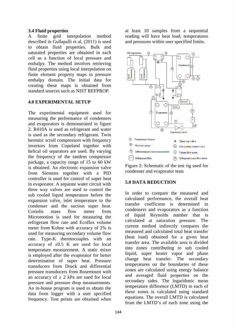
144

3.4 Fluid properties A finite grid interpolation method described in Gullapalli et al, (2011) is used to obtain fluid properties. Bulk and saturated properties are obtained in each cell as a function of local pressure and enthalpy. The method involves retrieving fluid properties using local interpolation on finite element property maps in pressure enthalpy domain. The initial data for creating these maps is obtained from standard sources such as NIST REFPROP. 4.0 EXPERIMENTAL SETUP The experimental equipment used for measuring the performance of condensers and evaporators is demonstrated in figure 2. R410A is used as refrigerant and water is used as the secondary refrigerant. Twin hermitic scroll compressors with frequency invertors from Copeland together with helical oil separators are used. By varying the frequency of the tandem compressor package, a capacity range of 15 to 60 kW is obtained. An electronic expansion valve from Siemens together with a PID controller is used for control of super heat in evaporator. A separate water circuit with three way valves are used to control the sub cooled liquid temperature before the expansion valve, inlet temperature to the condenser and the suction super heat. Coriolis mass flow meter from Micromotion is used for measuring the refrigerant flow rate and Ecoflux volume meter from Kohne with accuracy of 2% is used for measuring secondary volume flow rate. Type-K thermocouples with an accuracy of ±0.5 K are used for local temperature measurement. A static mixer is employed after the evaporator for better determination of super heat. Pressure transducers from Druck and differential pressure transducers from Rosemount with an accuracy of ± 2 kPa are used for local pressure and pressure drop measurements. An in-house program is used to obtain the data from logger with a user specified frequency. Test points are obtained when

at least 10 samples from a sequential reading will have heat load, temperatures and pressures within user specified limits.

Figure 2: Schematic of the test rig used for condenser and evaporator tests 5.0 DATA REDUCTION In order to compare the measured and calculated performance, the overall heat transfer coefficient is determined in condensers and evaporators as a function of liquid Reynolds number that is calculated at saturation pressure. The current method indirectly compares the measured and calculated total heat transfer (heat load) obtained for a given heat transfer area. The available area is divided into zones contributing to sub cooled liquid, super heater vapor and phase change heat transfer. The secondary temperatures on the boundaries of these zones are calculated using energy balance and averaged fluid properties on the secondary sides. The logarithmic mean temperature difference (LMTD) in each of these zones is calculated using standard equations. The overall LMTD is calculated from the LMTD’s of each zone using the

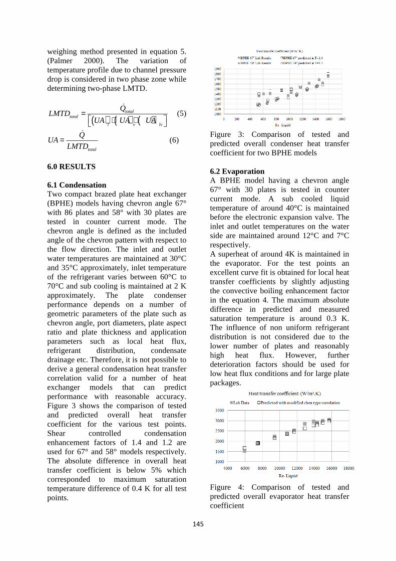
145

weighing method presented in equation 5. (Palmer 2000). The variation of temperature profile due to channel pressure drop is considered in two phase zone while determining two-phase LMTD.

( ) ( ) ( )total

total

l v lv

QLMTD

UA UA UA= + +

ɺ

(5)

total

QUA

LMTD=

ɺ

(6)

6.0 RESULTS 6.1 Condensation Two compact brazed plate heat exchanger (BPHE) models having chevron angle 67° with 86 plates and 58° with 30 plates are tested in counter current mode. The chevron angle is defined as the included angle of the chevron pattern with respect to the flow direction. The inlet and outlet water temperatures are maintained at 30°C and 35°C approximately, inlet temperature of the refrigerant varies between 60°C to 70°C and sub cooling is maintained at 2 K approximately. The plate condenser performance depends on a number of geometric parameters of the plate such as chevron angle, port diameters, plate aspect ratio and plate thickness and application parameters such as local heat flux, refrigerant distribution, condensate drainage etc. Therefore, it is not possible to derive a general condensation heat transfer correlation valid for a number of heat exchanger models that can predict performance with reasonable accuracy. Figure 3 shows the comparison of tested and predicted overall heat transfer coefficient for the various test points. Shear controlled condensation enhancement factors of 1.4 and 1.2 are used for 67° and 58° models respectively. The absolute difference in overall heat transfer coefficient is below 5% which corresponded to maximum saturation temperature difference of 0.4 K for all test points.

Figure 3: Comparison of tested and predicted overall condenser heat transfer coefficient for two BPHE models 6.2 Evaporation A BPHE model having a chevron angle 67° with 30 plates is tested in counter current mode. A sub cooled liquid temperature of around 40°C is maintained before the electronic expansion valve. The inlet and outlet temperatures on the water side are maintained around 12°C and 7°C respectively. A superheat of around 4K is maintained in the evaporator. For the test points an excellent curve fit is obtained for local heat transfer coefficients by slightly adjusting the convective boiling enhancement factor in the equation 4. The maximum absolute difference in predicted and measured saturation temperature is around 0.3 K. The influence of non uniform refrigerant distribution is not considered due to the lower number of plates and reasonably high heat flux. However, further deterioration factors should be used for low heat flux conditions and for large plate packages.

Figure 4: Comparison of tested and predicted overall evaporator heat transfer coefficient

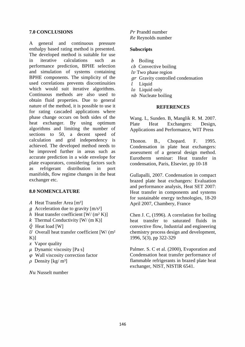
146

7.0 CONCLUSIONS A general and continuous pressure enthalpy based rating method is presented. The developed method is suitable for use in iterative calculations such as performance prediction, BPHE selection and simulation of systems containing BPHE components. The simplicity of the used correlations prevents discontinuities which would suit iterative algorithms. Continuous methods are also used to obtain fluid properties. Due to general nature of the method, it is possible to use it for rating cascaded applications where phase change occurs on both sides of the heat exchanger. By using optimum algorithms and limiting the number of sections to 50, a decent speed of calculation and grid independency is achieved. The developed method needs to be improved further in areas such as accurate prediction in a wide envelope for plate evaporators, considering factors such as refrigerant distribution in port manifolds, flow regime changes in the heat exchanger etc. 8.0 NOMENCLATURE Heat Transfer Area [m²] Acceleration due to gravity [m/s²] ℎ Heat transfer coefficient [W/ (m² K)] Thermal Conductivity [W/ (m K)] Heat load [W] Overall heat transfer coefficient [W/ (m² K)] Vapor quality Dynamic viscosity [Pa s] Wall viscosity correction factor Density [kg/ m³] Nusselt number

Prandtl number Reynolds number Subscripts Boiling Convective boiling Two phase region Gravity controlled condensation Liquid Liquid only Nucleate boiling

REFERENCES Wang. L, Sunden. B, Manglik R. M. 2007. Plate Heat Exchangers: Design, Applications and Performance, WIT Press Thonon. B., Chopard. F. 1995. Condensation in plate heat exchangers: assessment of a general design method. Eurotherm seminar: Heat transfer in condensation, Paris, Elsevier, pp 10-18 Gullapalli, 2007. Condensation in compact brazed plate heat exchangers: Evaluation and performance analysis, Heat SET 2007: Heat transfer in components and systems for sustainable energy technologies, 18-20 April 2007, Chambery, France Chen J. C, (1996). A correlation for boiling heat transfer to saturated fluids in convective flow, Industrial and engineering chemistry process design and development, 1996, 5(3), pp 322-329 Palmer. S. C et al. (2000), Evaporation and Condensation heat transfer performance of flammable refrigerants in brazed plate heat exchanger, NIST, NISTIR 6541.

147

Paper 5

Condensation in compact brazed plate heat exchangers: Evaluation and performance analysis Conference Presentation: Heat transfer in components and systems for sustainable energy technologies, 18-20 April 2007, Chambery, France

148

Heat SET 2007 Heat Transfer in Components and Systems

for Sustainable Energy Technologies 18-20 April 2007, Chambery, France

CONDENSATION IN COMPACT BRAZED PLATE HEAT EXCHANGERS: EVALUATION AND PERFORMANCE ANALYSIS

VijayaSekhar Gullapalli Heat Transfer Research, SWEP International AB,

P. O. Box 105, Landskrona, Sweden S-261 22 vijaya.sekhargullapalli@swep.net

ABSTRACT Condensation in compact brazed plate heat exchangers is influenced by a number of parameters, such as, geometry of the plate (chevron angle, pitch), Reynolds number of the flow and condensate drainage effect etc. Nusselt theory of condensation over a flat plate along with the intensification factors gives a reasonable approximation of the heat transfer in brazed plate heat exchangers in gravity governed regime. Methods using two phase multipliers and enhancement factors are used in evaluating the heat transfer coefficient in the shear controlled regime. This paper presents a comparative study of various correlations used to obtain the local heat transfer coefficient and the influence of the plate geometry on these correlations. Performance of the compact condenser is obtained locally by dividing the flow path into a number of elements. Keywords: Condensation, Brazed plate heat exchangers 1 INTRODUCTION 1.1 Compact brazed plate heat exchangers Compact brazed plate heat exchangers (CBE) are constructed by brazing together a series of corrugated plates in vacuum. Stainless steel plates with four apertures serving as inlet and outlet ports are pressed to the designed pattern. These plates are then arranged to form alternate flow passages with spacing of 1.3 to 6.4 mm [5]. During the vacuum brazing process, a braze joint is formed at every contact point between the base material and brazing material, usually copper or nickel. The brazing process results in a strong unit which is suitable for operating pressures above 30 bar. Using a thick frame, the CBE can be used up to operating pressures of 120 bar in supercritical applications. The close temperature approach (1-2 °C), small internal volume, higher heat transfer coefficients, compactness, elimination of cross contamination, lower cost and the ability to withstand higher operating pressures etc favor the use of CBE’s in refrigeration applications. The required heat capacity can be obtained by adjusting the number of plates. Asymmetric plate packages are also used to meet the demand of heat transfer rate and allowed pressure drop.

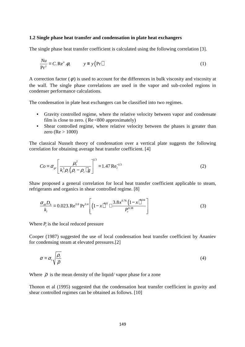
149

1.2 Single phase heat transfer and condensation in plate heat exchangers The single phase heat transfer coefficient is calculated using the following correlation [3].

( ).Re . , PrPr

ny

NuC y yφ= ≡ (1)

A correction factor (φ ) is used to account for the differences in bulk viscosity and viscosity at the wall. The single phase correlations are used in the vapor and sub-cooled regions in condenser performance calculations. The condensation in plate heat exchangers can be classified into two regimes.

• Gravity controlled regime, where the relative velocity between vapor and condensate film is close to zero. (Re<800 approximately)

• Shear controlled regime, where relative velocity between the phases is greater than zero (Re > 1000)

The classical Nusselt theory of condensation over a vertical plate suggests the following correlation for obtaining average heat transfer coefficient. [4]

( )

1 32

1 33

1.47 Relgr l

l l l v

Cok g

µαρ ρ ρ

− = = −

(2)

Shaw proposed a general correlation for local heat transfer coefficient applicable to steam, refrigerants and organics in shear controlled regime. [8]

( ) ( )0.040.760.80.8 0.4

0.38

3.8 10.023.Re Pr 1sh h

l r

x xDx

k P

α −= − +

(3)

Where rP is the local reduced pressure

Cooper (1987) suggested the use of local condensation heat transfer coefficient by Ananiev for condensing steam at elevated pressures.[2]

ll

ρα αρ

= (4)

Where ρ is the mean density of the liquid/ vapor phase for a zone Thonon et al (1995) suggested that the condensation heat transfer coefficient in gravity and shear controlled regimes can be obtained as follows. [10]

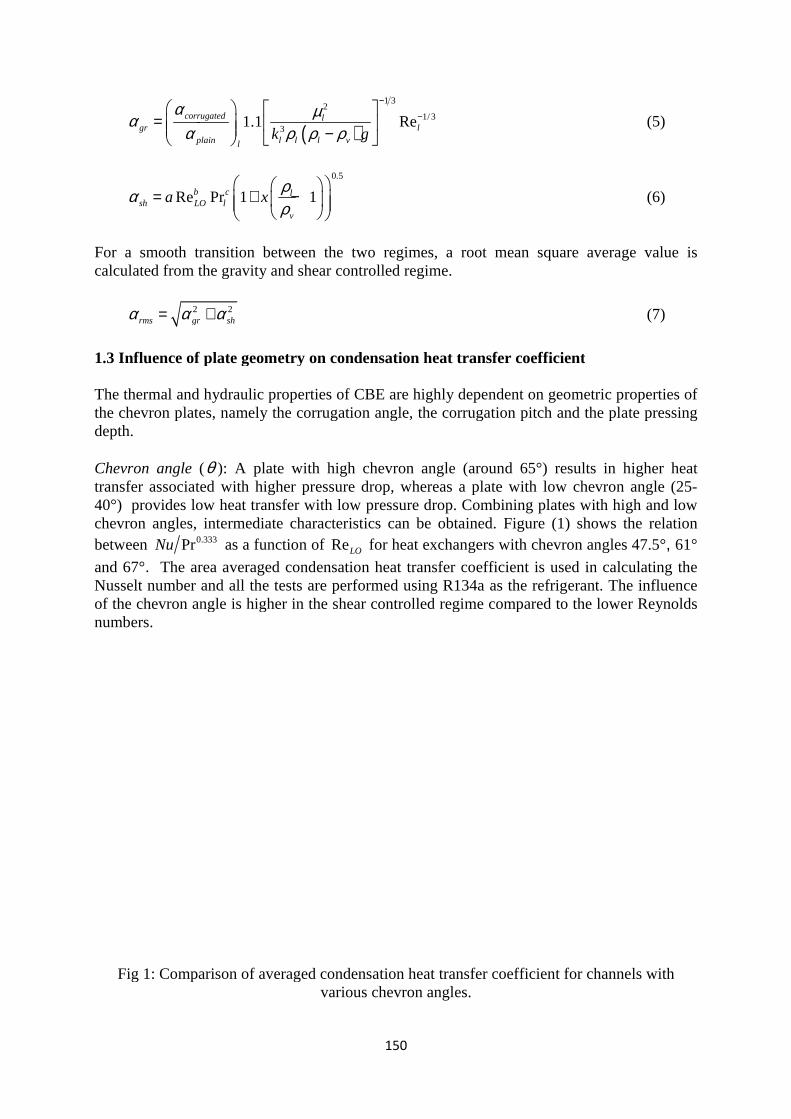
corrugatedgr l

plain l l l v

αα

α ρ ρ ρ

=

Re Pr 1 1b csh LO la xα = + −

For a smooth transition between the two regimes, a root mean square average value is calculated from the gravity and shear controlled regime.

2 2rms gr shα α α= +

1.3 Influence of The thermal and hydraulic properties of CBE are highly dependent on geometric properties of the chevron plates, namely the corrugation angle, the corrugation pitch and the plate pressing depth. Chevron angle transfer associated with higher pressure drop, whereas a plate with low chevron angle (2540°) provides low heat transfer with low pressure drop.chevron angles, intermediate characteristics can be obtained. Figure (1) shows the relation between 0.333PrNu

and 67°. The area averaged condensation heat transfer coefficient is used in calculating the Nusselt number and all the tests are performed using R134a as the refrigerant. The influence of the chevron angle is higher in the shear controlled regime comnumbers.

Fig 1: Comparison of averaged condensation heat transfer coefficient for channels with

150

( )

1 32

31.1 Recorrugated l

gr lplain l l l vl

k g

µα ρ ρ ρ

− −

0.5

Re Pr 1 1b c lsh LO l

v

a xρρ

= + −

For a smooth transition between the two regimes, a root mean square average value is calculated from the gravity and shear controlled regime.

2 2rms gr shα α α= +

1.3 Influence of plate geometry on condensation heat transfer coefficient

The thermal and hydraulic properties of CBE are highly dependent on geometric properties of the chevron plates, namely the corrugation angle, the corrugation pitch and the plate pressing

(θ ): A plate with high chevron angle (around 65°) results in higher heat transfer associated with higher pressure drop, whereas a plate with low chevron angle (2540°) provides low heat transfer with low pressure drop.chevron angles, intermediate characteristics can be obtained. Figure (1) shows the relation

0.333Pr as a function of ReLO for heat exchangers with chevron angles 47.5°

The area averaged condensation heat transfer coefficient is used in calculating the Nusselt number and all the tests are performed using R134a as the refrigerant. The influence of the chevron angle is higher in the shear controlled regime com

Fig 1: Comparison of averaged condensation heat transfer coefficient for channels with

various chevron angles.

150

1 3

1/31.1 Regr l−

For a smooth transition between the two regimes, a root mean square average value is calculated from the gravity and shear controlled regime.

plate geometry on condensation heat transfer coefficient

The thermal and hydraulic properties of CBE are highly dependent on geometric properties of the chevron plates, namely the corrugation angle, the corrugation pitch and the plate pressing

): A plate with high chevron angle (around 65°) results in higher heat transfer associated with higher pressure drop, whereas a plate with low chevron angle (2540°) provides low heat transfer with low pressure drop. Combining plates with high and low chevron angles, intermediate characteristics can be obtained. Figure (1) shows the relation

for heat exchangers with chevron angles 47.5°

The area averaged condensation heat transfer coefficient is used in calculating the Nusselt number and all the tests are performed using R134a as the refrigerant. The influence of the chevron angle is higher in the shear controlled regime compared to the lower Reynolds

Fig 1: Comparison of averaged condensation heat transfer coefficient for channels with

various chevron angles.

(5)

(6)

For a smooth transition between the two regimes, a root mean square average value is

(7)

The thermal and hydraulic properties of CBE are highly dependent on geometric properties of the chevron plates, namely the corrugation angle, the corrugation pitch and the plate pressing

): A plate with high chevron angle (around 65°) results in higher heat transfer associated with higher pressure drop, whereas a plate with low chevron angle (25-

Combining plates with high and low chevron angles, intermediate characteristics can be obtained. Figure (1) shows the relation

for heat exchangers with chevron angles 47.5°, 61°

The area averaged condensation heat transfer coefficient is used in calculating the Nusselt number and all the tests are performed using R134a as the refrigerant. The influence

pared to the lower Reynolds

Fig 1: Comparison of averaged condensation heat transfer coefficient for channels with

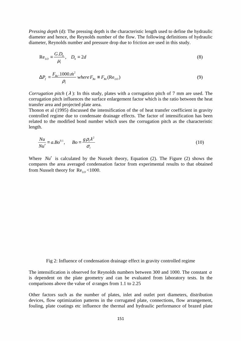
Pressing depth (d): The pressing depth is the characteristic length used to define the hydraulic diameter and hence, the Reynolds number of the flow. The following definitions of hydraulic diameter, Reynolds number and pressure drop due to friction are used in this stud

.Re , 2LO h

l

G D

µ= =

.1000.Ref Re Re LO

F mP where F F∆ = ≡

Corrugation pitchcorrugation pitch influences the surface enlargement factor whichtransfer area and projected plate area.Thonon et al (1995) discussed the intensification of the of heat transfer coefficient in gravity controlled regime due to condensate drainage effects. The factor of intensification has related to the modified bond number which uses the corrugation pitch as the characteristic length.

0.1. ,Nu

a Bo BoNu

= =′

Where Nu′ is calculated by the Nusselt theory, Equation (2). The Figure (2) shows the compares the area averaged condensation factor from experimental results to that obtained from Nusselt theory for

Fig 2: Influence of

The intensification is observed for Reynolds numbers between 300 and 1000. The constant is dependent on the plate geometry and can be evaluated from laboratory tests. In tcomparisons above the value of Other factors such as the number of plates, inlet and outlet port diameters, distribution devices, flow optimization patterns in the corrugated plate, connections, flow arfouling, plate coatings etc influence the thermal and hydraulic performance of brazed plate

151

(d): The pressing depth is the characteristic length used to define the hydraulic diameter and hence, the Reynolds number of the flow. The following definitions of hydraulic diameter, Reynolds number and pressure drop due to friction are used in this stud

.Re , 2h

LO hl

G DD d

µ= =

2.1000.

(Re )f Re Re LOl

F mP where F F

ρ∆ = ≡

ɺ

Corrugation pitch (λ ): In this study, plates with a corrugation pitch of 7 mm are used. The corrugation pitch influences the surface enlargement factor whichtransfer area and projected plate area. Thonon et al (1995) discussed the intensification of the of heat transfer coefficient in gravity controlled regime due to condensate drainage effects. The factor of intensification has related to the modified bond number which uses the corrugation pitch as the characteristic

20.1. , l

l

ga Bo Bo

ρ λσ

= =

is calculated by the Nusselt theory, Equation (2). The Figure (2) shows the compares the area averaged condensation factor from experimental results to that obtained from Nusselt theory for ReLO <1000.

Fig 2: Influence of condensation drainage effect in gravity controlled regime

The intensification is observed for Reynolds numbers between 300 and 1000. The constant is dependent on the plate geometry and can be evaluated from laboratory tests. In tcomparisons above the value of aranges from 1.1 to 2.25

Other factors such as the number of plates, inlet and outlet port diameters, distribution devices, flow optimization patterns in the corrugated plate, connections, flow arfouling, plate coatings etc influence the thermal and hydraulic performance of brazed plate

151

(d): The pressing depth is the characteristic length used to define the hydraulic diameter and hence, the Reynolds number of the flow. The following definitions of hydraulic diameter, Reynolds number and pressure drop due to friction are used in this stud

(Re )

): In this study, plates with a corrugation pitch of 7 mm are used. The

corrugation pitch influences the surface enlargement factor which is the ratio between the heat

Thonon et al (1995) discussed the intensification of the of heat transfer coefficient in gravity controlled regime due to condensate drainage effects. The factor of intensification has related to the modified bond number which uses the corrugation pitch as the characteristic

is calculated by the Nusselt theory, Equation (2). The Figure (2) shows the compares the area averaged condensation factor from experimental results to that obtained

condensation drainage effect in gravity controlled regime

The intensification is observed for Reynolds numbers between 300 and 1000. The constant is dependent on the plate geometry and can be evaluated from laboratory tests. In t

ranges from 1.1 to 2.25

Other factors such as the number of plates, inlet and outlet port diameters, distribution devices, flow optimization patterns in the corrugated plate, connections, flow arfouling, plate coatings etc influence the thermal and hydraulic performance of brazed plate

(d): The pressing depth is the characteristic length used to define the hydraulic diameter and hence, the Reynolds number of the flow. The following definitions of hydraulic diameter, Reynolds number and pressure drop due to friction are used in this study.

(8)

(9)

): In this study, plates with a corrugation pitch of 7 mm are used. The is the ratio between the heat

Thonon et al (1995) discussed the intensification of the of heat transfer coefficient in gravity controlled regime due to condensate drainage effects. The factor of intensification has been related to the modified bond number which uses the corrugation pitch as the characteristic

(10)

is calculated by the Nusselt theory, Equation (2). The Figure (2) shows the compares the area averaged condensation factor from experimental results to that obtained

condensation drainage effect in gravity controlled regime

The intensification is observed for Reynolds numbers between 300 and 1000. The constant ais dependent on the plate geometry and can be evaluated from laboratory tests. In the

Other factors such as the number of plates, inlet and outlet port diameters, distribution devices, flow optimization patterns in the corrugated plate, connections, flow arrangement, fouling, plate coatings etc influence the thermal and hydraulic performance of brazed plate

152

heat exchangers. The parametric study of influence of geometry can be obtained from, for example, [1] [6] [9] 2 CALCULATION PROCEDURES 2.1 Calculation of area averaged heat transfer coefficient The weighted method suggested by Palmer (2000) is used to determine the area averaged heat transfer coefficient. [7] The total heat load is the sum of heat loads in condensation, de-superheating and sub-cooling zones.

total sub cond desupQ Q Q Q= + +ɺ ɺ ɺ ɺ (11)

The log-mean temperature difference, LMTD, for the entire heat exchanger is determined from the weighted average of LMTDs for each segment.

1

.avg total

sub cond desup

Q Q QLMTD Q

LMTD LMTD LMTD

− ′= + +

ɺ ɺ ɺ

(12)

2.2 Discretized performance analysis of condensers The flow path in the both sides of the heat exchanger is divided into one-dimensional elements. Each element is characterized by the total mass flow rate and extends between two nodes. The nodes are characterized by local enthalpy, pressure and vapor quality. A system of nonlinear equations are developed applying the following set of equations at each element and node, which are then solved using a semi-explicit method. For each element representing the flow in channels,

( )2

1n n Wn element

n

dhm T T

dzα

=

= Π −∑ɺ (13)

f gr a

dPP P P

dz= ∆ + ∆ + ∆ (14)

For each node,

( ) 0phases

m =∑ ɺ (15)

The acceleration, gravity and friction components in the total pressure drop are evaluated from standard definitions of two phase friction factor multiplier, void fraction and mean density. The fluid properties are obtained locally as functions of the thermodynamic state parameters in elements and nodes. VijayaSekhar (2005) suggested that using the knowledge of the thermal and hydraulic behavior of individual CBE components, the discretized performance analysis can be used for an accurate modeling of temperature and mass flow mal-distribution in heat exchangers. [11]

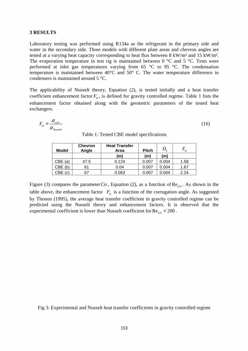
3 RESULTS Laboratory testing was performed using R134a as thwater in the secondary side. Three models with different plate areas and chevron angles are tested at a varying heat capacity corresponding to heat flux between 8 kW/m² and 15 kW/m². The evaporation temperature in testperformed at inlet gas temperatures varying from 65 °C to 95 °C. The condensation temperature is maintained between 40°C and 50° C. The water temperature difference in condensers is maintained around 5 ° The applicability of Nusselt theory, Equation (2), is tested initially and a heat transfer coefficient enhancement factor

enhancement factor obtained along with the geometric parameters of the tested heat exchangers.

corr

Nusselt

Fαα

α=

Model

CBE (a)CBE (b)CBE (c)

Figure (3) compares the parameter

table above, the enhancement factor

by Thonon (1995), the average heat transfer coefficient in gravity controlled regime can be predicted using the Nusselt theory and enhancement factors. It is observed that the experimental coefficient i

Fig 3: Experimental and Nusselt heat transfer coefficients in gravity controlled regime

153

Laboratory testing was performed using R134a as thwater in the secondary side. Three models with different plate areas and chevron angles are tested at a varying heat capacity corresponding to heat flux between 8 kW/m² and 15 kW/m². The evaporation temperature in test rig is maintained between 0 °C and 5 °C. Tests were performed at inlet gas temperatures varying from 65 °C to 95 °C. The condensation temperature is maintained between 40°C and 50° C. The water temperature difference in condensers is maintained around 5 °C.

The applicability of Nusselt theory, Equation (2), is tested initially and a heat transfer coefficient enhancement factorFα , is defined for gravity controlled regime. Table 1 lists the

enhancement factor obtained along with the geometric parameters of the tested heat

Nusselt

Table 1: Tested CBE model specifications

Model Chevron

Angle Heat Transfer

Area (m)

CBE (a) 47.5 0.124CBE (b) 61 0.04 CBE (c) 67 0.063

Figure (3) compares the parameterCo , Equation (2), as a function of

table above, the enhancement factor Fα is a function of the corrugation angle. As suggested

by Thonon (1995), the average heat transfer coefficient in gravity controlled regime can be predicted using the Nusselt theory and enhancement factors. It is observed that the experimental coefficient is lower than Nusselt coefficient for

Fig 3: Experimental and Nusselt heat transfer coefficients in gravity controlled regime

153

Laboratory testing was performed using R134a as the refrigerant in the primary side and water in the secondary side. Three models with different plate areas and chevron angles are tested at a varying heat capacity corresponding to heat flux between 8 kW/m² and 15 kW/m².

rig is maintained between 0 °C and 5 °C. Tests were performed at inlet gas temperatures varying from 65 °C to 95 °C. The condensation temperature is maintained between 40°C and 50° C. The water temperature difference in

The applicability of Nusselt theory, Equation (2), is tested initially and a heat transfer is defined for gravity controlled regime. Table 1 lists the

enhancement factor obtained along with the geometric parameters of the tested heat

Table 1: Tested CBE model specifications

Heat Transfer Pitch hD Fα

(m) (m) 0.124 0.007 0.004 1.58

0.007 0.004 1.670.063 0.007 0.004 2.24

, Equation (2), as a function ofReLO . As shown in the

is a function of the corrugation angle. As suggested

by Thonon (1995), the average heat transfer coefficient in gravity controlled regime can be predicted using the Nusselt theory and enhancement factors. It is observed that the

s lower than Nusselt coefficient forRe 200LO < .

Fig 3: Experimental and Nusselt heat transfer coefficients in gravity controlled regime

e refrigerant in the primary side and water in the secondary side. Three models with different plate areas and chevron angles are tested at a varying heat capacity corresponding to heat flux between 8 kW/m² and 15 kW/m².

rig is maintained between 0 °C and 5 °C. Tests were performed at inlet gas temperatures varying from 65 °C to 95 °C. The condensation temperature is maintained between 40°C and 50° C. The water temperature difference in

The applicability of Nusselt theory, Equation (2), is tested initially and a heat transfer is defined for gravity controlled regime. Table 1 lists the

enhancement factor obtained along with the geometric parameters of the tested heat

(16)

Fα

1.58 1.67 2.24

. As shown in the

is a function of the corrugation angle. As suggested

by Thonon (1995), the average heat transfer coefficient in gravity controlled regime can be predicted using the Nusselt theory and enhancement factors. It is observed that the

Fig 3: Experimental and Nusselt heat transfer coefficients in gravity controlled regime

The discretized method is used for performance analysis of condensers and the correlations proposed by Shaw, Cooper (1987) and Thonon (1995) are used for obtaining the local heat transfer coefficients. The enhancement factor,

Thonon correlation in gravity controlled regime. The following figures present the comparison of correlations for area averaged heat transfer coefficient for CBE (a) and CBE (c) models in Table 1.

Fig 4: Local condensation heat transfer coefficient for 47.5° plate using various correlations

Fig 5: Local condensation heat transfer coefficient for 67° plate using various correlations 4 CONCLUSIONS The study presents the influence of condensate drainage effect and enhancement of heat transfer coefficient in gravity controlled regime as a function of the plate chevron angle. The enhancement factors are then used to calculate local heat transfer coeffiperformance analysis tool. Correlations proposed by Cooper (1987) and Shah over predict the heat transfer in condensers. Using the evaluated enhancement factors, the general design

154

The discretized method is used for performance analysis of condensers and the correlations proposed by Shaw, Cooper (1987) and Thonon (1995) are used for obtaining the local heat transfer coefficients. The enhancement factor,

Thonon correlation in gravity controlled regime. The following figures present the comparison of correlations for area averaged heat transfer coefficient for CBE (a) and CBE (c) models in Table 1.

ondensation heat transfer coefficient for 47.5° plate using various correlations

Fig 5: Local condensation heat transfer coefficient for 67° plate using various correlations

4 CONCLUSIONS

The study presents the influence of condensate drainage effect and enhancement of heat transfer coefficient in gravity controlled regime as a function of the plate chevron angle. The enhancement factors are then used to calculate local heat transfer coeffiperformance analysis tool. Correlations proposed by Cooper (1987) and Shah over predict the heat transfer in condensers. Using the evaluated enhancement factors, the general design

154

The discretized method is used for performance analysis of condensers and the correlations proposed by Shaw, Cooper (1987) and Thonon (1995) are used for obtaining the local heat

Fα obtained in previous section is used in the

Thonon correlation in gravity controlled regime. The following figures present the comparison of correlations for area averaged heat transfer coefficient for CBE (a) and CBE

ondensation heat transfer coefficient for 47.5° plate using various correlations

Fig 5: Local condensation heat transfer coefficient for 67° plate using various correlations

The study presents the influence of condensate drainage effect and enhancement of heat transfer coefficient in gravity controlled regime as a function of the plate chevron angle. The enhancement factors are then used to calculate local heat transfer coefficient in a discretized performance analysis tool. Correlations proposed by Cooper (1987) and Shah over predict the heat transfer in condensers. Using the evaluated enhancement factors, the general design

The discretized method is used for performance analysis of condensers and the correlations proposed by Shaw, Cooper (1987) and Thonon (1995) are used for obtaining the local heat

ained in previous section is used in the

Thonon correlation in gravity controlled regime. The following figures present the comparison of correlations for area averaged heat transfer coefficient for CBE (a) and CBE

ondensation heat transfer coefficient for 47.5° plate using various correlations

Fig 5: Local condensation heat transfer coefficient for 67° plate using various correlations

The study presents the influence of condensate drainage effect and enhancement of heat transfer coefficient in gravity controlled regime as a function of the plate chevron angle. The

cient in a discretized performance analysis tool. Correlations proposed by Cooper (1987) and Shah over predict the heat transfer in condensers. Using the evaluated enhancement factors, the general design

155

method proposed by Thonon (1995) is suitable for predicting local heat transfer coefficient for Reynolds numbers under 1500. However, deviation is observed at higher Reynolds numbers. Further study would involve studying applicability of Thonon correlation at higher Reynolds numbers and using the discretized performance tool for glide refrigerants etc.

ACKNOWLEDGEMENT The development of simulation tool and experimental testing has been done at Heat Transfer Research, SWEP International AB, Sweden. NOMENCLATURE A Heat transfer area m² Bo Bond number - C Constant - Co Condensation Number -

pC Specific heat capacity J/(kg.K)

hD Hydraulic diameter m

d Pressing depth m Fα Enhancement Factor -

G Mass flux kg/ (s.m²) g Gravitational acceleration m/s² h Specific enthalpy J/kg

fgh Latent heat J/kg

k Thermal conductivity W/(m.K) LMTD Log-mean temperature difference K mɺ Mass flow rate kg/sec n Constant - NU Nusselt number - P Pressure Pa Pr Prandtl number -

rP Reduced Pressure -

Qɺ Heat load W Re Reynolds Number - T Temperature K U Overall heat transfer coefficient W/(m².K) x Vapor Quality - y Prandtl exponent - z Coordinate m α Heat transfer coefficient W/(m².K) λ Corrugation pitch m µ Dynamic viscosity Pa. s φ Viscosity correction factor - Π Perimeter m ρ Density kg/m³

156

σ Surface Tension N/m θ Chevron angle ° Index a Acceleration component cond Condensation zone desup De-super heating zone element Averaged value in discretized element f Friction gr Gravity controlled regime l Liquid LO Liquid only rms Root mean square sh Shear controlled regime sub Sub-cooled zone v Vapor W Wall REFERENCES [1] Arun Muley., Raj. M. Manglik., 1997, Enhanced heat transfer characteristics of single phase flow in plate heat exchangers with mixed chevron plates, Journal of enhanced heat transfer, Vol.4, pp. 187-201 [2] Cooper. A., 1987, Condensation of steam in plate heat exchangers, AIChE Symp.70:17-177 [3] Fredrik Strömer, 2002, SSP – Single phase algorithms, SWEP International AB, Landskrona, Sweden. [4] John. G. Collier., John. R. Thome., 1999, Convective boiling and condensation, Third edition, Oxford university press. [5] Kuppan. T., Heat exchanger design handbook, 2000, Marcel Dekker, Inc. [6] Mir-Akbar Hessami, 2003, An experimental investigation of the performance of cross-corrugated plate heat exchangers, Journal of enhanced heat transfer, Vol.10, No 4, p 379 [7] Palmer. S.C. et al., 2000, Evaporation and Condensation heat transfer performance of flammable refrigerants in a brazed plate heat exchanger, NIST, NISTIR 6541 [8] Srinivasan. V., Ramesh. K. Shah., 1997, Condensation in compact heat exchangers, Journal of enhanced heat transfer, Vol.4, pp. 237-256 [9] Thonon. B. et al., 1995, Recent research and development in plate heat exchangers, Journal of Enhanced Heat Transfer, Vol.2, Nos. 1-2, pp. 149.155 [10] Thonon. B., F. Chopard, 1995, Condensation in plate heat exchangers: assessment of a general design method, Eurotherm Seminar, Heat transfer in condensation, Paris, Elsevier, pp. 10-18 [11] Vijaya Sekhar. G., 2005, Component based performance analysis of compact brazed plate heat exchangers, Eurotherm 82, Numerical heat transfer 2005, Cracow, Poland. [12] Wang. L., et al, 2000, An experimental investigation of steam condensation in plate heat exchangers, International journal of heat exchangers, Volume 1, No.2.

157