Embed Size (px)
Citation preview

Institutionen för systemteknikDepartment of Electrical Engineering
Examensarbete
Estimation of Inter-cell Interference in 3GCommunication Systems
Examensarbete utfört i Reglerteknikvid Tekniska högskolan vid Linköpings universitet
av
Dan Gunning & Pontus Jernberg
LiTH-ISY-EX--11/4516--SE
Linköping 2011
Department of Electrical Engineering Linköpings tekniska högskolaLinköpings universitet Linköpings universitetSE-581 83 Linköping, Sweden 581 83 Linköping


Estimation of Inter-cell Interference in 3GCommunication Systems
Examensarbete utfört i Reglerteknikvid Tekniska högskolan i Linköping
av
Dan Gunning & Pontus Jernberg
LiTH-ISY-EX--11/4516--SE
Handledare: Ylva Jungisy, Linköpings universitet
Graham Goodwincdsc, University of Newcastle
Katrina Laucdsc, University of Newcastle
Examinator: Thomas Schönisy, Linköpings universitet
Linköping, 1 September, 2011


Avdelning, InstitutionDivision, Department
Division of Automatic ControlDepartment of Electrical EngineeringLinköpings universitetSE-581 83 Linköping, Sweden
DatumDate
2011-09-01
SpråkLanguage
� Svenska/Swedish� Engelska/English
�
�
RapporttypReport category
� Licentiatavhandling� Examensarbete� C-uppsats� D-uppsats� Övrig rapport�
�
URL för elektronisk versionhttp://www.control.isy.liu.se
http://urn.kb.se/resolve?urn=urn:nbn:se:liu:diva-71156
ISBN—
ISRNLiTH-ISY-EX--11/4516--SE
Serietitel och serienummerTitle of series, numbering
ISSN—
TitelTitle Estimation of Inter-cell Interference in 3G Communication Systems
FörfattareAuthor
Dan Gunning & Pontus Jernberg
SammanfattningAbstract
In this thesis the telecommunication problem known as inter-cell interferenceis examined. Inter-cell interference originates from users in neighboring cellsand affects the users in the own cell. The reason that inter-cell interference isinteresting to study is that it affects the maximum data-rates achievable in the3G network. By knowing the inter-cell interference, higher data-rates can bescheduled without risking cell-instability.
An expression for the coupling between cells is derived using basic physicalprinciples. Using the expression for the coupling factors a nonlinear modeldescribing the inter-cell interference is developed from the model of the power-control loop commonly used in the base stations. The expression describing thecoupling factors depends on the positions of users which are unknown. A quasidecentralized method for estimating the coupling factors using measurements ofthe total interference power is presented.
The estimation results presented in this thesis could probably be improved byusing a more advanced nonlinear filter, such as a particle filter or an ExtendedKalman filter, for the estimation. Different expressions describing the couplingfactors could also be considered to improve the result.
NyckelordKeywords inter-cell interference, thermal noise, Decision Feedback Equalizer, estimation, 3G,
Kalman filter, nonlinear model, quasi-decentralized estimator


AbstractIn this thesis the telecommunication problem known as inter-cell interference isexamined. Inter-cell interference originates from users in neighboring cells and af-fects the users in the own cell. The reason that inter-cell interference is interestingto study is that it affects the maximum data-rates achievable in the 3G network.By knowing the inter-cell interference, higher data-rates can be scheduled withoutrisking cell-instability.
An expression for the coupling between cells is derived using basic physical prin-ciples. Using the expression for the coupling factors a nonlinear model describingthe inter-cell interference is developed from the model of the power-control loopcommonly used in the base stations. The expression describing the coupling fac-tors depends on the positions of users which are unknown. A quasi decentralizedmethod for estimating the coupling factors using measurements of the total inter-ference power is presented.
The estimation results presented in this thesis could probably be improved byusing a more advanced nonlinear filter, such as a particle filter or an ExtendedKalman filter, for the estimation. Different expressions describing the couplingfactors could also be considered to improve the result.
v


Acknowledgments
This thesis has been performed at the University of Newcastle Australia at theCentre for Complex Dynamic Systems and Control. We would like to thank ev-eryone at the department, especially Professor Graham Goodwin and Dr. KatrinaLau without whom this thesis could not have been successfully completed. Wewould also like to acknowledge Ericsson for providing the motivation for this the-sis. We especially thank Professor Torbjörn Wigren and Dr. Erik Geijer Lundinfor their assistance. Thank you for all your help, patience and enthusiasm for theproject. It has been a very interesting and challenging project and we have learneda lot.
We would also like to thank our examiner Dr. Thomas Schön and our supervisorYlva Jung for all their support and encouragement.
Dan Gunning & Pontus JernbergNewcastle, July 2011
vii


Contents
1 Introduction 11.1 Purpose & Goals . . . . . . . . . . . . . . . . . . . . . . . . . . . . 11.2 Background . . . . . . . . . . . . . . . . . . . . . . . . . . . . . . . 2
1.2.1 The Evolution of 3G communicators . . . . . . . . . . . . . 21.2.2 Rate constraints . . . . . . . . . . . . . . . . . . . . . . . . 21.2.3 Power Control and Interference Model . . . . . . . . . . . . 4
1.3 Limitations . . . . . . . . . . . . . . . . . . . . . . . . . . . . . . . 51.4 Related research . . . . . . . . . . . . . . . . . . . . . . . . . . . . 5
2 Theory 72.1 Power control loop description and analysis . . . . . . . . . . . . . 7
2.1.1 Single cell, n equal users . . . . . . . . . . . . . . . . . . . . 82.1.2 Multiple cells, n equal users . . . . . . . . . . . . . . . . . . 9
2.2 Inter-cell model . . . . . . . . . . . . . . . . . . . . . . . . . . . . . 132.3 Loads . . . . . . . . . . . . . . . . . . . . . . . . . . . . . . . . . . 152.4 Stability - Multi-cell constraints . . . . . . . . . . . . . . . . . . . . 18
2.4.1 2-cell case . . . . . . . . . . . . . . . . . . . . . . . . . . . . 182.4.2 3-cell case . . . . . . . . . . . . . . . . . . . . . . . . . . . . 202.4.3 n-cell case . . . . . . . . . . . . . . . . . . . . . . . . . . . . 21
2.5 Stability - conservatism versus failure-rate . . . . . . . . . . . . . . 222.6 A linear model for estimating the coupling . . . . . . . . . . . . . . 232.7 Interference model . . . . . . . . . . . . . . . . . . . . . . . . . . . 25
2.7.1 Matrix inversion model . . . . . . . . . . . . . . . . . . . . 252.7.2 Iterative model . . . . . . . . . . . . . . . . . . . . . . . . . 262.7.3 Fast model . . . . . . . . . . . . . . . . . . . . . . . . . . . 272.7.4 Model with fixed λ . . . . . . . . . . . . . . . . . . . . . . . 28
2.8 State simulation . . . . . . . . . . . . . . . . . . . . . . . . . . . . 292.9 Kalman filter . . . . . . . . . . . . . . . . . . . . . . . . . . . . . . 312.10 Decision Feedback Equalizer . . . . . . . . . . . . . . . . . . . . . . 32
3 Results 333.1 Stability experiments . . . . . . . . . . . . . . . . . . . . . . . . . . 33
3.1.1 Experiment 1 . . . . . . . . . . . . . . . . . . . . . . . . . . 333.1.2 Experiment 2 . . . . . . . . . . . . . . . . . . . . . . . . . . 35
ix

x Contents
3.1.3 Experiment 3 . . . . . . . . . . . . . . . . . . . . . . . . . . 363.1.4 Experiment 4 . . . . . . . . . . . . . . . . . . . . . . . . . . 373.1.5 Experiment 5 . . . . . . . . . . . . . . . . . . . . . . . . . . 38
3.2 Estimation experiments . . . . . . . . . . . . . . . . . . . . . . . . 393.2.1 Experiment A . . . . . . . . . . . . . . . . . . . . . . . . . . 403.2.2 Experiment B . . . . . . . . . . . . . . . . . . . . . . . . . . 433.2.3 Experiment C . . . . . . . . . . . . . . . . . . . . . . . . . . 463.2.4 Experiment D . . . . . . . . . . . . . . . . . . . . . . . . . . 553.2.5 Experiment E . . . . . . . . . . . . . . . . . . . . . . . . . . 58
4 Concluding remarks 614.1 Conclusions . . . . . . . . . . . . . . . . . . . . . . . . . . . . . . . 614.2 Future work . . . . . . . . . . . . . . . . . . . . . . . . . . . . . . . 62
Bibliography 63
A Abbreviations 65
B Notation 66
C Matlab code for the estimation experiments 68

Chapter 1
Introduction
This chapter contains the purpose, goals and background of this thesis. It alsoincludes the limitations and a short description of similar research that has beendone before.
1.1 Purpose & GoalsThe purpose of this thesis is to better understand single cell and multi-cell in-terference in 3G mobile communication systems. The motivation for this is thatthe entire operation of 3G communication depends critically on interference. Thesources of interference are
• thermal noise on the receiver antennas.
• interference from other users in the same cell.
• self interference (auto interference).
• interference from users in other cells (part of this is the neighboring cellresponding to the own cell).
Some of these sources are known, some are partially known, some are assumedknown and some are completely unknown and therefore models are needed. Thesemodels are nonlinear and contain unknown parameters and random variables.There are also noisy measurements which are nonlinear functions of the statesof the model.
The goals of this thesis are to
1. Derive an expression for the coupling between cells.
2. Develop a nonlinear model for inter-cell interference.
3. Estimate coupling factors using measurements generated by the model.
1

2 Introduction
1.2 BackgroundThis section contains a brief history of the evolution of 3G communicators. It alsocontains some details concerning rate constraints, power control and interferencemodels.
1.2.1 The Evolution of 3G communicatorsMobile telephony started to become international in the early 1980s with the in-troduction of the analog NMT system (Nordic Mobile Telephony). NMT made itpossible for users traveling outside the area of their home operator to still receiveservice (roaming), which gave mobile phones a larger market. At this point mobiletelephones were still bulky and could only support standard phone calls.
During the mid 1980s digital communication made it possible to develop a secondgeneration communication system (2G) that could not only make phone calls butalso send and receive small amounts of data. This introduced the possibility tosend and receive e-mail and also added support for Short Message Services (SMS).The highest data rates in early 2G were 9.6 kbps. In the second half of the 1990snew technology made it possible to send packet data over the cellular system. Thisis usually called 2.5G.
An international standardization of cellular systems and a larger market for prod-ucts were two of the main driving forces behind the development of the third gen-eration communication system (3G). This system provided a higher-bandwidthradio interface which made new services, which were only implied in 2G and 2.5G,possible. Since the introduction of 3G, mobile devices have become multi-purposedevices, not only used for phone calls.
As the demand on data and Internet services for mobile devices has increased sohas the need for higher data rates. Therefore a main goal for the evolution of 3G isto achieve higher end-user data rates compared to what was possible in the earlierreleases of 3G. This includes a higher overall data rate for the whole cell area andalso a higher peak data rate. A few of the limiting factors for data rates are theavailable bandwidth, the signal power and the noise interfering with transmissions.
1.2.2 Rate constraintsAccording to Shannon’s capacity theorem [3] the maximum rate that can be sentover a channel can be determined by
T = BW · log2(1+ P
N). (1.1)
In (1.1), T is the channel capacity, BW is the available bandwidth, P is thereceived signal power and N is the noise power. The noise is assumed to be white

1.2 Background 3
and additive. The signal power can be written as P = Eb · R, where Eb is theenergy received per bit (J/bit) and R is the rate of data communication (bit/s).Also, the noise power can be expressed as N = φ0 ·BW where φ0 is the constantnoise power spectral density (W/Hz). This gives the inequality
R ≤ T = BW · log2(1+ Eb ·Rφ0 ·BW
).
Defining the bandwidth utilization β = R/BW gives the expression
R ≤ T = BW ·log2(1+Ebφ0·β)⇔ β ≤ log2(1+Eb
φ0·β)⇔ 2β − 1
β≤ Ebφ0.
This expresses the signal-to-noise ratio (SNR) needed to send data with a certainrate over a limited bandwidth. Thus, for bandwidth utilization larger than onethe minimum required Eb/φ0 increases quickly, see Figure 1.1. [2]
10−1
100
101
−5
0
5
10
15
20
Power−limitedregion
Band−limitedregion
β
Min
imum
Eb/φ
0 req
uire
d (d
B)
Figure 1.1. Minimum Eb/φ0 required at the receiver as a function of β.

4 Introduction
1.2.3 Power Control and Interference Model
The channel is affected by time variations in the channel gains (fading). Usersalso interfere with each other due to the fact that the codes used to separate theusers are not completely orthogonal. Another problem is that a user close to abase station may overpower a user who is further away (near-far effect). To solvethese problems the signal-to-interference ratio (SIR) for each user is monitored bya power control loop which adjusts the users transmission power to compensatefor variations in the channel conditions. The goal is to keep the received SIR atan approximately constant level to successfully transmit data. The control loopincreases the power for a user who experiences poor channel quality and decreasesit for a user who experiences good channel quality. At time k the user transmitsdata at a power of γ(k) ·p′(k), where γ(k) is a scaling factor called the power grantand p′(k) is the transmitted power. A users’ data-rate is determined by the powergrant. The received power on the control channel at the base station is given byp(k) = p′(k) · g(k), where g(k) is the fading gain. [9] Note that, in the rest of thisthesis, both linear and logarithmic scales (i.e. dB) are used. A bar − is used todenote a linear quantity.
The SIR S for user i at time k is given by
Si(k) = pi(k)Ii(k)
,
where Ii(k) is the interference to the user, and is given by
Ii(k) =∑
1≤j≤n,j 6=i
(1+γj(k))·pj(k)+α·(1+γi(k))·pi(k)+N0+Iother(k). (1.2)
In equation (1.2), (1+γj(k))·pj(k) is the interference from user j, α·(1+γi(k))·pi(k)is the interference from the user to itself (α is a constant) and Iother(k) is the in-terference from users in other cells. The parameter N0 is unknown and consistsof thermal noise and other sources of interference. [9]
By rewriting (1.2) as Ii(k) = C−(1−α)·(1+γi(k))·pi(k), where C =∑
1≤j≤n(1+γj(k))·pj(k)+N0 +Iother(k) it can be shown that N0 +Iother(k) is a scaling factorfor the total interference. Therefore, by estimating N0 + Iother(k) it is possible toget a better estimation of the interference Ii(k). This will give a better model touse for power control, which in turn makes higher data rates possible.
1.3 Limitations 5
1.3 LimitationsThe experiments on inter-cell interference are limited to the interaction betweentwo cells only. The reason for this is that at least two cells are needed to examinethe problem, but using more than two cells would just increase the difficulty ofinterpreting the results. However, the models and all the formulas have beendeveloped with an arbitrary number of cells in mind. Since there is no way tomeasure the coupling factors without geographical information about every userin a cell, the quality of the estimates can only be measured against simulations.Variations in the channel gain (fading) are not considered.
1.4 Related researchBoth [2] and [8] are good choices for better understanding mobile communications,especially the evolution of the 3G network and the techniques used. They also givea description of the background and the technical details surrounding data trans-fers in the 3G network. [2] also contains details concerning the upcoming LTEsystem. Relevant aspects and discussions on Universal Mobile Telecommunica-tion System (UMTS) power control using an automatic control framework aredescribed in [7].
The problem of estimating inter-cell interference is closely linked to the problem ofestimating the thermal noise level. One approach to the latter problem is describedin [14] where a nonlinear three stage algorithm is used. The only measurementrequired is the Received Total Wideband Power (RTWP). In the first stage aKalman filter is used to estimate a Gaussian Probability Density Function (PDF)of the estimated RTWP. In the next stage the PDF is further processed to producean estimate of the thermal noise power floor. The last stage of the algorithm usesthe estimated RTWP and the thermal noise power floor to compute the WidebandCode Division Multiple Access (WCDMA) load in a single cell. The algorithm isa workaround for the problem that the thermal noise power floor is not observabledue to neighbor cell interference. This algorithm is further developed in [12] toinclude inter-cell interference in a single Radio Base Station (RBS). To reducememory usage of the algorithm without compromising performance a recursivescheme to estimate the thermal noise power floor has been developed. This givesthe possibility to run several instances of the algorithm in parallel in the RBS. [13]
In [9] a nonlinear decoupling algorithm for the uplink of the WCDMA 3G cellularsystem is described. This is a way to combat the interference from users withinthe same cell. The paper shows that decoupling strategies lead to significant per-formance gains relative to the decentralized strategies used today.
The basic theory for constructing mathematical and physical models for a pro-cess as well as model validation and simulation can be found in [10]. A basicframework for stability analysis of Multiple-Input Multiple-Output (MIMO) sys-tems and nonlinear models is treated in [4]. A popular method for estimating

6 Introduction
unobservable (latent) states of a nonlinear model is to use a Particle filter (PF).The fundamental PF theory as well as its use in tracking applications is describedin [5]. The nonlinear filtering problem is also presented. In addition the articlecontains an overview of the Marginalized (often called Rao-Blackwellized) Parti-cle filter (MPF or RBPF) and a general framework of how PF can be applied tocomplex systems.

Chapter 2
Theory
This chapter describes the theoretical expressions and calculations that are laterused in the experiments in chapter 3. It also contains theory taken from literatureas well as models and mathematical expressions developed in this thesis.
2.1 Power control loop description and analysisTo control the SIR of a User Equipment (UE) within a cell in a mobile network,power control is used. The power control is commonly handled in a decentralizedmanner with one Single-Input Single-Output loop (SISO) for each UE. A simplifiedblock diagram of the power control loop for a single user is shown in Figure 2.1,where S∗ is the desired SIR for the user (in dB), p′(k) is the transmitted power,p(k) is the received power, g(k) is the channel gain, I(k) is interference powerand S(k) is the SIR at time k. A typical choice for the controller is K(q) =1. An alternative which has been considered in some detail in the literature isK(q) = 1/(1 + q−1 + ... + q−d+1) where d is the delay and the mobile stationG(q) = q−d/(1− q−1), (see [9] and the references therein).
S∗K(q) G(q)
Controller Mobile station
+
−
+
+
−
+
S(k)
g(k) I(k)
e(k) u(k) p′(k) p(k)
Desired SIR
Measured SIR
Figure 2.1. Power control loop for a single user.
7
8 Theory
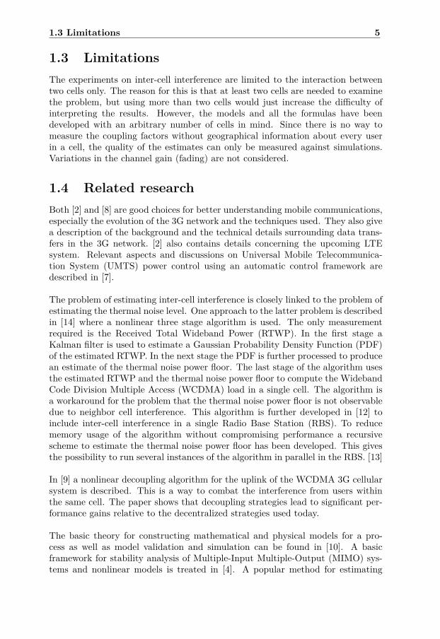
2.1.1 Single cell, n equal usersBy assuming d = 1 and g(k) = 0 the following can be derived
p(k + 1) = p(k) + u(k),u(k) = e(k),e(k) = S∗ − S(k),S(k) = p(k)− I(k).
For the case of n equal users I(k) = n · (1+γ(k)) ·p(k)+(α · (1+γ(k)) ·p(k)+N0),where α · (1 + γ(k)) · p(k) is the auto-interference or self-interference and N0 isthe thermal noise at the antenna. As noted in section 1.2.3 a bar denotes a linearquantity. This gives the expression p(k + 1) = p(k) + S∗ − S(k) = p(k) + S∗ −p(k) + I(k) = S∗ + I(k) which in linear scale becomes
p(k+1) = S∗ ·I(k) = S
∗ ·(α·(1+γ(k))·p(k)+N0). (2.1)
Equation (2.1) is a linear state-space representation of the system and can be re-written as p(k + 1) = A · p(k) + b, where A = S
∗ · α · (1 + γ(k)) and b = S∗ ·N0.
The poles of a system, which determine its stability properties, are given by theeigen-values of the matrix A [4]. By examining the eigenvalues for increasing val-ues of the power-grant γ it is possible to find the maximum value of γ before thesystem reaches instability. It is assumed that the data-rate is proportional to thepower grant and hence, maximizing the cell throughput is equivalent to maximiz-ing the sum of the users’ grants. In the case of n equal users (i.e. γi = γ), this isequivalent to maximizing γ.
The upper limit on the data-rate can also be estimated using the expression forsteady state power, described by
p = S∗ ·N0
1− (n− 1 + α) · (1 + γ) · S∗. (2.2)

2.1 Power control loop description and analysis 9
For the case of a single user (n = 1) Figure 2.2 shows the value of the powergrant γ that gives the highest achievable data-rate with these two approaches.As expected the two methods yield the same result and in this case instability isreached at γ = 212.
0 50 100 150 200 250−2
−1
0
1
2
Rea
l com
pone
nt o
f pol
e
0 50 100 150 200 250−5
0
5
10
15x 10
−9
Pow
er [m
W]
γ
Figure 2.2. Poles (top) and Power (bottom) for increasing power grant (γ) whereS
∗ = 1/64, α = 0.3 and n = 1.
Figure 2.4 shows the value of the power grant γ that gives the highest achievabledata-rate for n = 2. It also assumes that S∗1 = S
∗2 = 1/64 and α1 = α2 = 0.3. Just
as before the two approaches give the same result. As seen in the figure instabilityis reached at γ1 = γ2 = 49 which is earlier compared to the single-user case.
2.1.2 Multiple cells, n equal usersFor the case of users in neighboring cells Ii(k) = n · (1 + γi(k)) · pi(k) + αi · (1 +γi(k)) ·pi(k) +N0 + Iotherji(k), where Iotherji(k) is the interference from user j touser i. The resulting SISO-loop, for the case of two users, is shown in Figure 2.3,where ICl is a gain factor for how much user l interferes with the other user andHl is the interference transfer function for user l, in this case l = 1, 2.

10 Theory
S∗1
K1(q) G1(q)
Controller Mobile station
+
−
+
+
−
+
S1(k)
g1(k)
I1(k)
e1(k) u1(k) p′1(k) p1(k)
Desired SIR
Measured SIR
S∗2
K2(q) G2(q)
Controller Mobile station
+
−
+
+
−
+
S2(k)
g2(k)
I2(k)
e2(k) u2(k) p′2(k) p2(k)
Desired SIR
Measured SIR
H2
H1
IC2
IC1
Iother21(k)
Iother12(k)
N0
N0
Figure 2.3. The common SISO-loop for two users in neighboring cells.
Using the same assumptions as in the single-user case the following equations canbe derived
p1(k + 1) = p1(k) + u1(k),u1(k) = e1(k),e1(k) = S∗1 − S1(k),S1(k) = p1(k)− I1(k),
p2(k + 1) = p2(k) + u2(k),u2(k) = e2(k),e2(k) = S∗2 − S2(k),S2(k) = p2(k)− I2(k).

2.1 Power control loop description and analysis 11
The interference for the users, expressed in linear scale, are described by
I1(k) = α1 · (1 + γ1(k)) · p1(k) +N0 + Iother21(k),I2(k) = α2 · (1 + γ2(k)) · p2(k) +N0 + Iother12(k),
where
Iother21(k) = IC2 · (1 + γ2(k)) · p2(k),Iother12(k) = IC1 · (1 + γ1(k)) · p1(k).
In the same way as in the single-user case above, the linear recursive power equa-tions are given by
p1(k + 1) = S∗1 · (α1 · (1 + γ1(k)) · p1(k) +N0 + IC2 · (1 + γ2(k)) · p2(k)), (2.3)
p2(k + 1) = S∗2 · (α2 · (1 + γ2(k)) · p2(k) +N0 + IC1 · (1 + γ1(k)) · p1(k)). (2.4)
Rewriting (2.3) and (2.4) using vector notation gives the state-space equation
pk+1 = A ·pk +b. (2.5)
To find the maximum achievable data-rate before reaching instability the eigen-values of the matrix A in (2.5) are examined for equal increase of the power grantsγ1(k) and γ2(k) as well as IC1 = IC2 = 1. In other words the users interfere fullywith one another. The result can then be compared to the steady-state powergiven by (2.2) with n = 2.

12 Theory
0 50 100 150 200 250−2
−1
0
1
2
Rea
l com
pone
nt o
f pol
e
Pole 1Pole 2
0 50 100 150 200 250−1
0
1
2
3
4x 10
−9
Pow
er [m
W]
γ
Figure 2.4. Poles (top) and Power (bottom) for increasing power grant (γ) and n = 2.

2.2 Inter-cell model 13
2.2 Inter-cell modelTo get a basic understanding of the effects of inter-cell interference, consider thesimple example in Figure 2.5.
−400 −200 0 200 400 600 800 1000 1200 1400
−400
−200
0
200
400
UE 1
UE 2
UE 1
Cell 1 Cell 2
Distance x [m]
Dis
tanc
e y
[m]
Figure 2.5. Two cells with a total of three users. Base stations are illustrated with acircle.
By writing the power equations on state-space form as in (2.5) we get the followingA-matrix[
S∗11 · α11 · (1 + γ11(k)) S
∗11 · (1 + γ12(k)) S
∗11 · IC21−1 · (1 + γ21(k))
S∗12 · (1 + γ11(k)) S
∗12 · α12 · (1 + γ12(k)) S
∗12 · IC21−1 · (1 + γ21(k))
S∗21 · IC11−2 · (1 + γ11(k)) S
∗21 · IC12−2 · (1 + γ12(k)) S
∗21 · α21 · (1 + γ21(k))
]
Let the positions of the UEs and the base stations as well as the radius of thecells be known. To determine the value of ICij−l, which is the interference gainfrom user j in cell i to cell l, the power reaching the own base station, P 1, andthe power reaching the other base station, P 2, are needed. If it is assumed thatthere is no fading these two quantities can be expressed as in equation (2.6) andequation (2.7) using the inverse square law.
P 1 = P ij
d2ij−i
, (2.6)
P 2 = P ij
d2ij−l
, (2.7)
where P ij is the transmission power from user j in cell i, dij−i is the distance fromuser j in cell i to the base station in cell i and dij−l is the distance from user j incell i to the base station in cell l.

14 Theory
The coupling factors can then be expressed as the ratio P 2/P 1 as in
ICij−l = (dij−idij−l
)2. (2.8)
Figure 2.6 shows a map of the resulting IC-values when two cells with the sameradius are placed next to each other with no overlap (as in Figure 2.5). The Figureshows the IC-values as a function of position for the cell on the left hand side.
Figure 2.6. The value of the coupling factors depending on the UE position in the cell.
By assuming that the positions of the users and base stations are known it is pos-sible to calculate the A-matrix and examine the eigenvalues for different values ofγij . Furthermore the results in Figure 2.7 assume that S∗ij are equal for all [i, j], nofading, αij are equal for all [i, j], γij increases equally for all users in all cells andthat the setup is the same as in Figure 2.5. Instability is reached for γ = 45 whichis almost the same as in Figure 2.4 where there are two users and the interferencegain IC = 1. If full coupling would be assumed instability is reached at γ = 27.
The simple case described above can be extended to a more general case with anarbitrary number of users in each cell. The structure of the resulting A-matrix isshown in Figure 2.8.

2.3 Loads 15
0 50 100 150 200 250−2
−1.5
−1
−0.5
0
0.5
1
1.5
2
γ
Rea
l com
pone
nt o
f pol
e
Figure 2.7. Pole placement for increasing γ values where S∗11 = S
∗12 = S
∗21 = 1/64,
α11 = α12 = α21 = 0.3 and n = 3.
Self-interference elements
Elements for interference from users in the same cell
Elements for interference from users in other cells
Figure 2.8. The structure of the general A-matrix.
2.3 LoadsIn section 2.1 the eigenvalues of the A-matrix were calculated in order to get thestability properties of the system. An alternative to this is to calculate the loadLi(k) for i = 1 . . . n where n is the number of users in the cell, as described in(2.9). It is known that, for a single cell, if
∑ni=1 Li(k) < 1, the system is stable [8].
This stability criterion is valid under the assumption that the total interferencepower is arbitrarily large, which is shown at the end of this section.
Li(k) = (1 + γi(k))1
Si(k)+ (1− αi) · (1 + γi(k))
(2.9)

16 Theory
The stability criterion∑ni=1 Li(k) < 1 can be derived by looking at the SIR-
equation for user i in cell l
Sli(k) = P li(k)I li(k)
. (2.10)
Let Cl be the total interference power for cell l. Then Cl is given by
Cl(k) =n1∑i=1
(1+γi(k))·P li(k)+Iotherml(k)+N0l. (2.11)
It follows that I li(k) = Cl(k)− (1− αli) · (1 + γli(k)) · P li(k).
Equation (2.12) is then given by rearranging (2.10) as described below
Sli(k) = P li(k)Cl(k)− (1− αli) · (1 + γli(k)) · P li(k)
⇔ Cl(k)− (1− αli) · (1 + γli(k)) · P li(k) = P li(k)Sli(k)
⇔ Cl(k) =(
1Sli(k)
+ (1− αli) · (1 + γli(k))· P li(k)
⇔ P li(k) = Cl(k)1
Sli(k)+ (1− αli) · (1 + γli(k))
. (2.12)
Let Iotherml(k) be the inter-cell interference from cell m to cell l described by
Iotherml(k) =∑∀m,m 6=l
nm∑j=1
ICmj−l · (1 + γmj(k)) · Pmj(k). (2.13)

2.3 Loads 17
Inserting (2.13) into equation (2.11) gives
Cl(k) =n1∑i=1
(1 + γli(k)) · P li(k)
+∑∀m,m6=l
nm∑j=1
ICmj−l · (1 + γmj(k)) · Pmj(k) +N0l (2.14)
Equation (2.15) is given by inserting (2.12) into (2.14).
Cl(k) =nl∑i=1
(1 + γli(k)) · Cl(k)1
Sli(k)+ (1− αli) · (1 + γli(k))
+∑∀m,m 6=l
nm∑j=1
ICmj−l ·(1 + γmj(k)) · Cm(k)
1Smj(k)
+ (1− αmj) · (1 + γmj(k))+N0l
⇔ Cl(k) =nl∑i=1
Lli(k) · Cl(k) +∑∀m,m 6=l
nm∑j=1
ICmj−l · Lmj(k) · Cm(k) +N0l
⇔nl∑i=1
Lli(k) +∑∀m,m6=l
nm∑j=1
ICmj−l · Lmj(k) · Cm(k)Cl(k)
+ N0l
Cl(k)= 1 (2.15)
Normally the contribution from the other cells, Iotherml(k), is not taken into ac-count. It is then easy to see that the stability criterion
∑ni=1 Li(k) < 1 is only
valid if Cl(k) is arbitrarily large. However, if Iotherml(k) is taken into account andCl(k) is assumed to be arbitrarily large the stability of cell m will be affected. Thereason for this is that the factor Cm(k)/Cl(k) in (2.15) will be inverted. Clearlyit is not possible to have
∑ni=1 Li(k) arbitrarily close to 1 when the contribution
from the other cells is considered.

18 Theory
2.4 Stability - Multi-cell constraintsThis section describes different approaches to derive necessary and sufficient con-ditions for stability that consider inter-cell interference.
2.4.1 2-cell caseIn this section the 2-cell case, which is a special case of (2.15) is examined. Thetotal interference power for cell 1 and cell 2 are given by (2.16) and (2.17) respec-tively.
C1(k)−
a1︷ ︸︸ ︷n1∑i=1
L1i(k) ·C1(k)−
b1︷ ︸︸ ︷n2∑j=1
IC2j−1 · L2j(k) ·C2(k) = N01 (2.16)
C2(k)−n2∑j=1
L2j(k)︸ ︷︷ ︸a2
·C2(k)−n1∑i=1
IC1i−2 · L1i(k)︸ ︷︷ ︸b2
·C1(k) = N02 (2.17)
By writing (2.16) and (2.17) on matrix-form we get
[1− a1 −b1−b2 1− a2
]︸ ︷︷ ︸
A
·[C1C2
]︸ ︷︷ ︸
C
=[N01N02
]︸ ︷︷ ︸
N
Solving this expression for C gives:
C = 1det(A) ·
[1− a2 b1b2 1− a1
]︸ ︷︷ ︸
A−1
·N (2.18)
For a feasible solution to (2.18), which is necessary for stability, C > 0 must holdas it is not possible to have a negative total interference power. SinceN, a1, a2, b1,b2 > 0 the solution is only positive if a1, a2 < 1 and det(A) > 0. The determinantis given by
det(A) = (1− a1) · (1− a2)− b1 · b2.
The condition that det(A) > 0 gives the inequality
b1 · b2 < (1− a1) · (1− a2). (2.19)
Together with a1, a2 < 1, (2.19) forms a necessary and sufficient condition forstability.

2.4 Stability - Multi-cell constraints 19
If full coupling from the other cell is assumed, b1 = a2 and b2 = a1 hold. Usingthis, the following sufficient condition for stability can be derived
a1 · a2 < (1− a1) · (1− a2)⇔ a1 · a2 < 1 + a1 · a2 − a1 − a2
⇔ a1 + a2 < 1. (2.20)
The sufficient stability condition above also holds in the case of coupling less thanone, since
b1 · b2 ≤ a1 · a2 < (1− a1) · (1− a2).
If the coupling is greater than one a necessary condition for stability is that eitherb1 or b2 has to be less than one. They can not both be greater than one at thesame time.
As mentioned above, C has to be greater than zero for a feasible solution. Thismeans that A−1 has to be elementwise positive. Using Perron-Frobenius theorem,see [11], it can be shown that
(I−B)−1 ≥ 0 iff ρ(B) = |λmax(B)| < 1, (2.21)
where B is a nonnegative matrix. It is not hard to see that the A-matrix can bewritten in the form
A =
I−[a1 b1b2 a2
]︸ ︷︷ ︸
B
, where B is a nonnegative matrix.
The necessary and sufficient condition given by (2.21) states that if the spectralradius of B, ρ(B) which is equal to the absolute of the largest eigenvalue of B, isless than one, then A−1 is positive and we have a feasible solution for C.

20 Theory
The eigenvalues of B are calculated as below
det(B− λ · I) =∣∣∣∣a1 − λ b1b2 a2 − λ
∣∣∣∣ = 0
⇔ (a1 − λ) · (a2 − λ)− b1 · b2 = 0⇔ a1 · a2 − a1 · λ− a2 · λ+ λ2 − b1 · b2 = 0
⇔ (λ− a1 + a2
2 )2 − (a1 + a2
2 )2 + a1 · a2 − b1 · b2 = 0
⇔ λ = a1 + a2
2 ±√
(a1 + a2
2 )2 − a1 · a2 + b1 · b2.
It can now be seen that the largest absolute eigenvalue is given for the case of fullcoupling. In this case,
λ1 = a1 + a2,
λ2 = 0.
Hence, λmax(B) ≤ a1 + a2. This together with Perron-Frobenius theorem givesthe sufficient condition a1 + a2 < 1, which is the same as in (2.20).
2.4.2 3-cell caseIn this section the 3-cell case is analyzed and stability conditions are derived.The calculations are similar to the ones in 2.4.1 but since there are 3 cells thecalculations are a bit more tedious. C is calculated as in (2.18) but in this casethe A-matrix is given by
A =
1− a1 −b12 −b13−b21 1− a2 −b23−b31 −b32 1− a3
By rewriting A on the following form, (2.21) can once again be used.
A =
I−a1 b12 b13b21 a2 b23b31 b32 a3
︸ ︷︷ ︸
B
, where B is a nonnegative matrix.

2.4 Stability - Multi-cell constraints 21
The eigenvalues of B are calculated as below
det(B− λ · I) = −λ3 + (a1 + a2 + a3) · λ2
+ (−a1 · a2 − a1 · a3 − a2 · a3 + b12 · b21 + b13 · b31 + b23 · b32) · λ+ a1 · a2 · a3 + b21 · b32 · b13 + b31 · b12 · b23
− a1 · b23 · b32 − a2 · b13 · b31 − a3 · b12 · b21
= 0.
If full coupling is assumed the eigenvalues are
λ1 = a1 + a2 + a3,
λ2 = λ3 = 0.
But what happens to the eigenvalues when the coupling is less than one? Is itpossible to get a matrix with an absolute eigenvalue greater than in the case offull coupling? The short answer is no.
For a matrix where the elements in each column are a scaling (between 0 and 1)of that columns’ diagonal element it can be shown, using Gersgorin discs, that thelargest absolute eigenvalue occurs when all the scaling factors are equal to one.Details on Gersgorin discs can be found in [11].
In other words, it can be concluded that a1 + a2 + a3 < 1 is a sufficient conditionfor stability in the case of full coupling (or less).
2.4.3 n-cell caseSince the A-matrix always has the same structure, the necessary and sufficientcondition given by (2.21) as well as the sufficient condition a1 + a2 + · · ·+ an < 1are valid also in the n-cell case.
One might be tempted to make things more simple by only considering two cells ata time (pairwise stability). However, it can be shown that even if a cell has pairwisestability with all of its neighboring cells the macro-cell can still be unstable. Inother words pairwise stability is not a sufficient condition for stability.

22 Theory
2.5 Stability - conservatism versus failure-rateThe sufficient stability condition a1 + a2 + · · ·+ an < 1 is quite conservative giventhe fact that it is not possible to have full coupling with more than one neighbor.The purpose of the experiments in this section is to find out whether it wouldbe a good idea to estimate the coupling factor from one cell to another. Thissection assumes a total of two cells. The modified stability condition used in thisexperiment is given by
a1 + µ · a2 < ε, (2.22)
where µ is a scaling factor between 0 and 1 and ε is a threshold.
Let µ be defined as
µi =ni∑j=1
ICij−lni
, (2.23)
where ICij−l is the coupling factor user j in cell i affects cell l with.
Let us now simulate the case where three UEs with grants between 5 and 30 areplaced randomly in each cell. Stability is then checked by analyzing the poles ofthe system. The left hand side of equation (2.22) is also calculated using equa-tion (2.23). This simulation is then repeated for a total of 10 000 times. Usingthe simulation data an ε, as well as a false alarm probability, that gives a misseddetection probability of 0.1% can be calculated. The result of the simulation isε = 0.97 and a false alarm probability of 0.45%.
From this we may conclude that knowing the µ-parameter of a cell is very usefulwhen scheduling the loads in each cell.

2.6 A linear model for estimating the coupling 23
2.6 A linear model for estimating the couplingIn this section the linear model that will be used for estimating the coupling factorsis described. Equation (2.15) shows that the total interference power for a cell canbe written as
Cl(k) =nl∑i=1
Lli(k) · Cl(k) +∑∀m,m6=l
nm∑j=1
ICmj−l · Lmj(k) · Cm(k) +N0l,
where nl and nm are the number of UEs in the cells l and m.
Let us now look at the two-cell case and let us assume that the coupled load fromthe other cell can be expressed using only one coupling factor instead of one foreach UE. The equation above can then be written as
C1(k) =
a1(k)︷ ︸︸ ︷n1∑i=1
L1i(k) ·C1(k) + µ2(k) ·
a2(k)︷ ︸︸ ︷n2∑j=1
L2j(k) ·C2(k) +N01,
C2(k) =n2∑j=1
L2j(k) · C2(k) + µ1(k) ·n1∑i=1
L1i(k) · C1(k) +N02. (2.24)
Since C1(k) and C2(k) can be measured and a1(k) and a2(k) are assigned by thescheduler and therefore known, let
y(k) =[C1(k)C2(k)
]be the measurements and (2.25)
x(k) =
µ1(k)µ2(k)N01(k)N02(k)
be the states. (2.26)

24 Theory
Let us assume that the time update of the first two states can be described as asemi-random walk and that the time update of the last two states can be describedby a random walk as shown below
x1(k + 1) = ρ1 · x1(k) + ω1(k),x2(k + 1) = ρ2 · x2(k) + ω2(k),x3(k + 1) = x3(k) + ω3(k),x4(k + 1) = x4(k) + ω4(k),
where ρ1 and ρ2 are constants between 0 and 1 and ωi(k), i = 1, ..., 4, denotes theprocess noise.
This gives the linear state-space model
x(k + 1) =
ρ1 0 0 00 ρ2 0 00 0 1 00 0 0 1
︸ ︷︷ ︸
A
·x(k) + ω(k),
y(k) =
0 a2(k)·C2(k)1−a1(k) 0 1
1−a1(k) 0a1(k)·C1(k)
1−a2(k) 0 0 11−a2(k)
︸ ︷︷ ︸
C
·x(k) + v(k), (2.27)
which will be used to estimate the coupling factors. Note that v(k) is the mea-surement noise.

2.7 Interference model 25
2.7 Interference modelIn order to test the estimator, the system needs to be simulated. This involvesgenerating grants for the users, simulating the positions of the users, convertingthe grants and positions to loads and coupling factors, respectively, and then simu-lating the total interference response (for each cell) to the given loads and couplingfactors. In this section, four models which describe the interference response for agiven set of loads and coupling factors will be presented and evaluated. To makeit easier to compare the different models and draw conclusions there is only oneUE in each cell.
2.7.1 Matrix inversion modelThis simple model is a matrix inversion based on equation (2.18) which solves theequation for C1(k) and C2(k) given a matrix A. In this case
A =[
1− a1(k) −µ2(k) · a2(k)−µ1(k) · a1(k) 1− a2(k)
](2.28)
and we get the solution
[C1(k)C2(k)
]= 1det(A) ·
[1− a2(k) µ2(k) · a2(k)
µ1(k) · a1(k) 1− a1(k)
]︸ ︷︷ ︸
A−1
·[N01(k)N02(k)
](2.29)
To examine the dynamics of this model a step test was performed. As seen inFigure 2.9 the response is instantaneous which is a desired property.
0 5 10 15 20 25 30 35 40 45 500
0.2
0.4
0.6
0.8
1
Sample
Load
Load over time
Cell 1Cell 2
0 5 10 15 20 25 30 35 40 45 501
2
3
4
5
6x 10
−14
Sample
Pow
er [W
]
Total interference power over time
Cell 1Cell 2
Figure 2.9. Step response with coupling factors µ1 = µ2 = 0.2.

26 Theory
2.7.2 Iterative modelAnother way of modeling the interference is to iteratively use equation (2.24) as atime update.
C1(k + 1) = a1(k) · C1(k) + µ2(k) · a2(k) · C2(k) +N01
C2(k + 1) = a2(k) · C2(k) + µ1(k) · a1(k) · C1(k) +N02
This gives the dynamic step response shown in Figure 2.10. It can be seen that ittakes the model some time to rise to the new value.
0 5 10 15 20 25 30 35 40 45 500
0.2
0.4
0.6
0.8
1
Sample
Load
Load over time
Cell 1Cell 2
0 5 10 15 20 25 30 35 40 45 501
2
3
4
5
6x 10
−14
Sample
Pow
er [W
]
Total interference power over time
Cell 1Cell 2
Figure 2.10. Step response with coupling factors µ1 = µ2 = 0.2.

2.7 Interference model 27
2.7.3 Fast modelThe model given by equation (2.30) below, solves equation (2.24) for C1 and C2at each time instance and uses this as a time update,
C1(k + 1) = µ2(k) · a2(k) · C2(k)1− a1(k) + N01
1− a1(k)
C2(k + 1) = µ1(k) · a1(k) · C1(k)1− a2(k) + N02
1− a2(k) . (2.30)
The step response for this model is shown in Figure 2.11. As shown the modelreaches its final value faster than the model described in section 2.7.2. Thereforethis model is more suitable for cases where the multi-cell system has a relativelyfast response.
0 5 10 15 20 25 30 35 40 45 500
0.2
0.4
0.6
0.8
1
Sample
Load
Load over time
Cell 1Cell 2
0 5 10 15 20 25 30 35 40 45 501
2
3
4
5
6x 10
−14
Sample
Pow
er [W
]
Total interference power over time
Cell 1Cell 2
Figure 2.11. Step response with coupling factors µ1 = µ2 = 0.2.

28 Theory
2.7.4 Model with fixed λThis model, given by equation (2.31), can be seen as an extension of the modeldescribed in section 2.7.3 using a forgetting factor λ,
C1(k + 1) =
old info︷ ︸︸ ︷λ · C1(k) +
innovation︷ ︸︸ ︷(1− λ) · (µ2(k) · a2(k) · C2(k) +N01
1− a1(k) )
C2(k + 1) = λ · C2(k) + (1− λ) · (µ1(k) · a1(k) · C1(k) +N02
1− a2(k) ). (2.31)
Figure 2.12 shows the step response for this model. The value of the forgettingfactor determines how much the previous value affects the current value. A lowvalue makes the model more suitable for cases where the loads vary fast but alsomore sensitive to noise. A high value gives the opposite result.
0 5 10 15 20 25 30 35 40 45 500
0.2
0.4
0.6
0.8
1
Sample
Load
Load over time
Cell 1Cell 2
0 5 10 15 20 25 30 35 40 45 501
2
3
4
5
6x 10
−14
Sample
Pow
er [W
]
Total interference power over time
Cell 1Cell 2
Figure 2.12. Step response with coupling factors µ1 = µ2 = 0.2 and λ = 0.5.

2.8 State simulation 29
2.8 State simulationAs mentioned in section 2.7, simulations of the states are needed in order toproduce measurements of the total interference power. These measurements arelater used in the estimation of the states. The simulation has two neighboringcells, each containing a number of UEs. Both the positions and the grants of theUEs are random walks from random starting positions. Figure 2.13 contains anexample-run of the simulation showing the cells and the positions of the UEs.
−400 −200 0 200 400 600 800 1000 1200 1400
−400
−300
−200
−100
0
100
200
300
400Cell 1 Cell 2
UE positions
Distance x [m]
Dis
tanc
e y
[m]
Figure 2.13. Example-run of the simulation showing how the three UEs in each cellmove around. The UE positions have a standard deviation of 4 m/sample in each direc-tion.
The loads of the UEs in this example-run of the simulation are shown in Fig-ure 2.14. The magenta line shows the sum of the loads in the own cell. The blackline shows the total load, which is the sum of the loads in the own cell plus thecoupled loads from the other cell.
0 50 100 150 200 250 300 350 400 450 5000
0.2
0.4
0.6
0.8
1Loads over time in cell 1
Sample
Load
0 50 100 150 200 250 300 350 400 450 5000
0.2
0.4
0.6
0.8
1Loads over time in cell 2
Sample
Load
Figure 2.14. Example-run of the simulation showing the total load, sum of the loadsand the loads of the three UEs in each cell. The UE loads have a standard deviation of0.05 per sample.
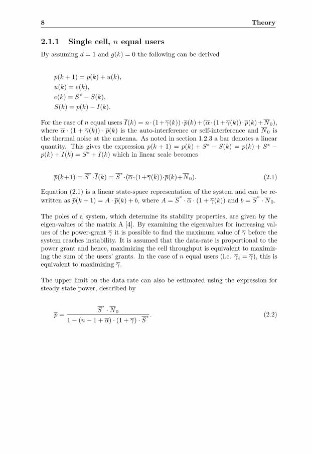
30 Theory
Using the position information of the UEs and the geometry described in equation(2.8) the coupling factors for each UE can be calculated. The result is shown inFigure 2.15. It is easy to see that this result is reasonable by looking at Figure 2.13together with Figure 2.6.
0 50 100 150 200 250 300 350 400 450 5000
0.2
0.4
0.6
0.8
1Observed IC values in cell 1
Sample
IC−
valu
e
0 50 100 150 200 250 300 350 400 450 5000
0.2
0.4
0.6
0.8
1Observed IC values in cell 2
Sample
IC−
valu
e
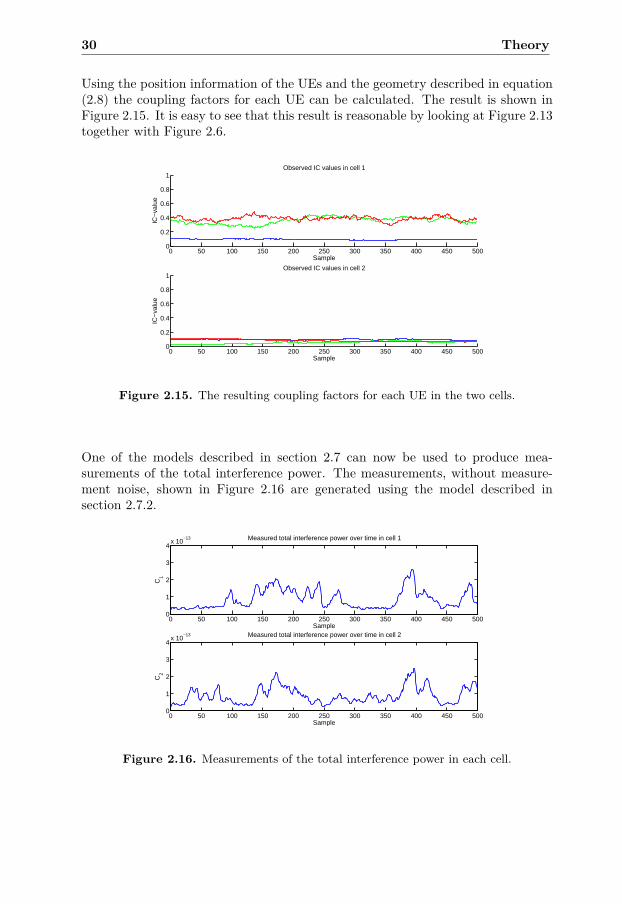
Figure 2.15. The resulting coupling factors for each UE in the two cells.
One of the models described in section 2.7 can now be used to produce mea-surements of the total interference power. The measurements, without measure-ment noise, shown in Figure 2.16 are generated using the model described insection 2.7.2.
0 50 100 150 200 250 300 350 400 450 5000
1
2
3
4x 10
−13 Measured total interference power over time in cell 1
Sample
C1
0 50 100 150 200 250 300 350 400 450 5000
1
2
3
4x 10
−13 Measured total interference power over time in cell 2
Sample
C2
Figure 2.16. Measurements of the total interference power in each cell.
2.9 Kalman filter 31
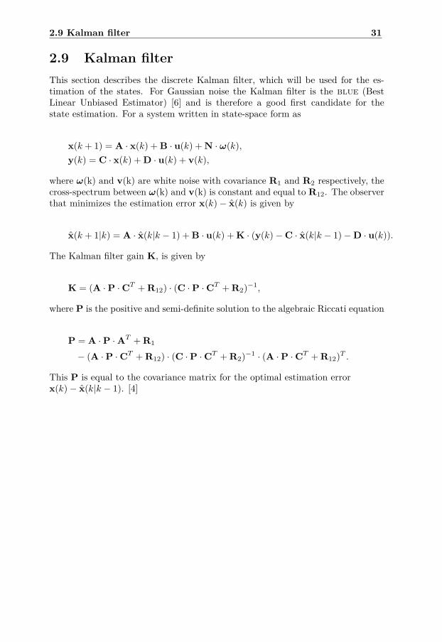
2.9 Kalman filterThis section describes the discrete Kalman filter, which will be used for the es-timation of the states. For Gaussian noise the Kalman filter is the blue (BestLinear Unbiased Estimator) [6] and is therefore a good first candidate for thestate estimation. For a system written in state-space form as
x(k + 1) = A · x(k) + B · u(k) + N · ω(k),y(k) = C · x(k) + D · u(k) + v(k),
where ω(k) and v(k) are white noise with covariance R1 and R2 respectively, thecross-spectrum between ω(k) and v(k) is constant and equal to R12. The observerthat minimizes the estimation error x(k)− x̂(k) is given by
x̂(k + 1|k) = A · x̂(k|k − 1) + B · u(k) + K · (y(k)−C · x̂(k|k − 1)−D · u(k)).
The Kalman filter gain K, is given by
K = (A ·P ·CT + R12) · (C ·P ·CT + R2)−1,
where P is the positive and semi-definite solution to the algebraic Riccati equation
P = A ·P ·AT + R1
− (A ·P ·CT + R12) · (C ·P ·CT + R2)−1 · (A ·P ·CT + R12)T .
This P is equal to the covariance matrix for the optimal estimation errorx(k)− x̂(k|k − 1). [4]

32 Theory
2.10 Decision Feedback EqualizerThere is always a risk that the estimates computed by the Kalman filter (KF) donot lie within the allowed limits of the states. This can lead to problems in futureestimates. To ensure that the estimates lie between the limits a Decision FeedbackEqualizer (DFE) can be used.[1] The DFE takes the estimated state vector, x̂(k),from the filter and if a state lies outside its allowed limits, it is saturated to theclosest of these limits. This new value, ˆ̂x(k), is set as the output and is also thefeedback to the filter. The block diagram of the DFE is shown in Figure 2.17.
KF sat(·)y(k) x̂(k) ˆ̂x(k)
z−1
Figure 2.17. Block diagram of the DFE.

Chapter 3
Results
In this chapter, the results and conclusions of the experiments performed duringthis thesis are presented.
3.1 Stability experimentsTo get a better understanding of inter-cell interference a number of experimentshave been conducted. The purpose of these experiments is to investigate how grantsize, position and number of UEs affect the stability of the cell.
3.1.1 Experiment 1In Figure 3.1, cell 1 contains 2 UEs with random positions and cell two containsone UE close to the border. The UE in cell 2 has a large power grant, γ(k) = 30.In cell 1, the power grants of the two UEs are increased equally until instability isreached. To get a good approximation of the γ(k), in cell 1, that gives instabilitythe simulation is run 2000 times, using different positions. Since the positions ofthe UEs in cell 1 change between each simulation they are not shown in the figure.As a reference to the results in this section, instability is reached for γ(k) = 49 forthe single-cell case with two UEs. The result of this special case is independent ofthe positions of the UEs in cell 1 and thus always the same no matter how manysimulations are run.
33

34 Results
−400 −200 0 200 400 600 800 1000 1200 1400
−400
−200
0
200
400
30
Cell 1 Cell 2
Distance x [m]
Dis
tanc
e y
[m]
Figure 3.1. Experiment 1, a UE close to the border.
Calculating the mean µ and variance σ2 of the γ(k), in cell 1, that causes instabilityover the 2000 simulations gives
µ = 44.8960,σ2 = 5.9221.
If the power grant in cell 2 is increased from 30 to 40 the results are
µ = 43.5065,σ2 = 10.3621.
By comparing the results from the two cases above it is seen that with an increasein the power grant in cell 2 there is also in increase in the variance.
Consider the case in Figure 3.1 again but increase the number of UEs in cell 1from two to three. This gives the following results
µ = 25.4475,σ2 = 1.0988.
This shows not only a decrease in the mean but more interestingly a large decreasein variance.
Reducing the radius of cell 1 from 500m to 250m gives the results below
µ = 43.6955,σ2 = 5.8997.

3.1 Stability experiments 35
These results are very similar to the original case in Figure 3.1, but more inter-estingly the value of IC21−1 has increased from 0.67 to 2.25. This is equivalent toadding 1.58 users, with the same grant as the user in cell 2, in cell 1. A possibleexplanation for the similar µ and σ values is that although the contribution fromthe user in cell 2 to cell 1 has increased the contribution from the users in cell 1to cell 2 has decreased.
3.1.2 Experiment 2To investigate how the position of the cells affect the stability, consider the case inFigure 3.2 where a UE belonging to cell 2 is placed in the intersection of the twocells. Note that the UE is closer to the base station in cell 1 than the base stationin cell 2, i.e. IC21−1 > 1.
−400 −200 0 200 400 600 800 1000 1200 1400
−400
−300
−200
−100
0
100
200
300
400
30
Cell 1 Cell 2
Distance x [m]
Dis
tanc
e y
[m]
Figure 3.2. Experiment 2, a UE belonging to cell 2 in the intersection of the two cells.
The results of this case are shown below. Experiments show that the varianceincreases even more if the overlap is made bigger while the mean decreases.
µ = 40.6455,σ2 = 24.3940.

36 Results
3.1.3 Experiment 3Let us now see what happens if the position of the UE in cell 2 is changed inaccordance with to Figure 3.3 and cell 1 contains two UEs.
−400 −200 0 200 400 600 800 1000 1200 1400
−400
−200
0
200
400
30
Cell 1 Cell 2
Distance x [m]
Dis
tanc
e y
[m]
Figure 3.3. Experiment 3, a UE far from the border.
The results of these changes are
µ = 48.0165,σ2 = 0.2764.
This shows that the position of the UE has a significant impact on both mean andvariance i.e. the contribution from a UE to the inter-cell interference decreaseswith the distance from the neighboring base station.
3.1 Stability experiments 37
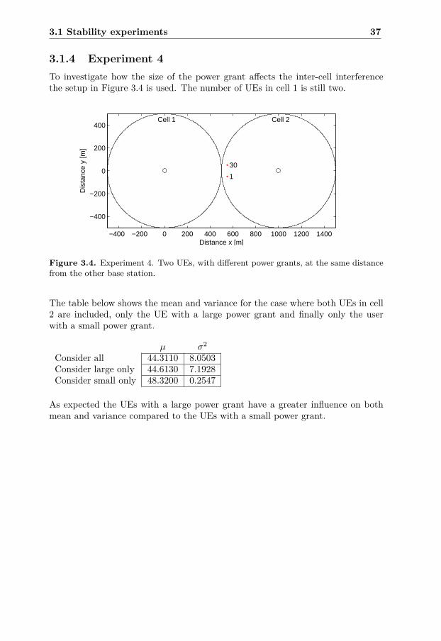
3.1.4 Experiment 4To investigate how the size of the power grant affects the inter-cell interferencethe setup in Figure 3.4 is used. The number of UEs in cell 1 is still two.
−400 −200 0 200 400 600 800 1000 1200 1400
−400
−200
0
200
400
1
30
Cell 1 Cell 2
Distance x [m]
Dis
tanc
e y
[m]
Figure 3.4. Experiment 4. Two UEs, with different power grants, at the same distancefrom the other base station.
The table below shows the mean and variance for the case where both UEs in cell2 are included, only the UE with a large power grant and finally only the userwith a small power grant.
µ σ2
Consider all 44.3110 8.0503Consider large only 44.6130 7.1928Consider small only 48.3200 0.2547
As expected the UEs with a large power grant have a greater influence on bothmean and variance compared to the UEs with a small power grant.

38 Results
3.1.5 Experiment 5To further compare the influence of different power grants as well as differentdistances the setup in Figure 3.5 is used.
−400 −200 0 200 400 600 800 1000 1200 1400
−400
−200
0
200
400
1 30
Cell 1 Cell 2
Distance x [m]
Dis
tanc
e y
[m]
Figure 3.5. Experiment 5, two UEs with different positions and power grants.
The results of the experiment are shown in the table below.
µ σ2
Consider all 47.6655 0.5779Consider large only 47.9975 0.2926Consider small only 48.3600 0.2665
This experiment shows that it is not only the size of the power grant, but also thedistance to the opposite base station, that determines the final contribution to theinter-cell interference. Therefore it is important that also UEs with small powergrants and short distances are taken into account.

3.2 Estimation experiments 39
3.2 Estimation experimentsThere are many parameters that affect the accuracy of the estimation of the statevector. To be able to evaluate the result of the quasi-decentralized estimationstrategy, a series of tests has been conducted. The notation used for the functionsin the experiments in these sections is explained in the list below.
Sim - the simulation described in section 2.8.
G - the linear model in section 2.6.
C - the output matrix derived in section 2.6.
KF - the Kalman filter described in section 2.9.
DFE - the DFE explained in section 2.10.
M1 - the matrix inversion model in section 2.7.1.
M2 - the iterative model in section 2.7.2.
M3 - the fast model in section 2.7.3.
M4 - the model with fixed λ in section 2.7.4.
The simulation run in Sim has one user in each of the two cells. This makes thestates µ1 and µ2 coincide with the IC-values calculated using equation (2.8). TheUEs move around with a standard deviation of 1.5 m in each direction and theirloads vary with a standard deviation of 0.05. The parameters N01 and N02 areassumed constant with the value −107 dBm [12]. In order to make the estimatedcoupling factors more visible in the innovation the measurements are scaled witha factor of 1014 to have an order of magnitude one before they are passed to theC-matrix and the Kalman filter. Note that this implies that N01 and N02 are alsoscaled and that the plots show the scaled versions. In order to avoid making theestimates too slow the constants ρ1 and ρ2 in the linear model are set to 0.98, avalue found through trial and error. The matrices Q, R and P0 mentioned in thefollowing sections refer to the covariance for the process noise, measurement noiseand initial state covariance.

40 Results
3.2.1 Experiment AThe purpose of this experiment is to investigate the performance of the quasi-decentralized estimation strategy in ideal conditions. The setup is shown in Fig-ure 3.6. The loads are taken from the simulation and the coupling factors fromthe linear model. They are then used in the matrix inversion model to producethe measurements. Note that there is no measurement noise in this experiment.Since the C-matrix needs a measurement of the total interference power in theother cell in order to estimate the total interference power in the own cell, themeasurements need to be passed to the C-matrix. The reason that the measure-ments are passed separately to the C-matrix and the Kalman filter is that in laterexperiments measurement noise will be added in between these.
KF
y(k)
x̂(k)
z−1
M1
Sim
G
l(k)
µ(k)
C
Figure 3.6. Block diagram of the experiment.
The matrices Q, R and P0 greatly influence the quality of the estimates. Forthis setup the Q-matrix is chosen to match the process noise used in the modelto generate the coupling factors. In order to make the Kalman filter put a lot oftrust into the measurements the R-matrix is made small. Finally, since the initialguesses of the states are set to the true value of the states, the P0-matrix is madesmall.
Q =
2.5e-6 0 0 0
0 2.5e-6 0 00 0 1e-8 00 0 0 1e-8
,R =[1e-4 0
0 1e-4
]
P0 =
1e-1 0 0 0
0 1e-1 0 00 0 1e-1 00 0 0 1e-1

3.2 Estimation experiments 41
The results for this setup are shown in Figure 3.7, 3.8, 3.9 and 3.10.
0 50 100 150 200 250 300 350 400 450 5000
0.2
0.4
0.6
0.8
1Load over time in cell 1
Sample
Load
0 50 100 150 200 250 300 350 400 450 5000
0.2
0.4
0.6
0.8
1Load over time in cell 2
Sample
Load
Figure 3.7. Loads over time in the two cells. The total loads are shown in black andthe loads of the UEs are shown in blue.
0 50 100 150 200 250 300 350 400 450 500−0.4
−0.2
0
0.2
Sample
µ 1
µ1 over time in cell 1
True µ
1
Estimated µ1
0 50 100 150 200 250 300 350 400 450 500−0.4
−0.2
0
0.2
Sample
µ 2
µ2 over time in cell 2
True µ
2
Estimated µ2
Figure 3.8. True (blue) and estimated (green) coupling factors using the matrix inver-sion model.

42 Results
0 50 100 150 200 250 300 350 400 450 5001.5
2
2.5
3
3.5
N01
over time in cell 1
Sample
N01
True N
01
Estimated N01
0 50 100 150 200 250 300 350 400 450 5001.5
2
2.5
3
3.5
N02
over time in cell 2
Sample
N02
True N
02
Estimated N02
Figure 3.9. True (blue) and estimated (green) thermal noise power using the matrixinversion model.
0 50 100 150 200 250 300 350 400 450 5000
5
10
15
20
25Measured total interference power over time in cell 1
Sample
C1
0 50 100 150 200 250 300 350 400 450 5000
5
10
15
20
25Measured total interference power over time in cell 2
Sample
C2
Figure 3.10. Measured total interference power over time using the matrix inversionmodel.
Conclusions
As expected the estimates are quite good since the coupling factors are generatedusing the same Q-matrix as in the Kalman filter, i.e. the process noise is known.However, as seen in Figure 3.8 the estimates are sometimes outside the allowedinterval, [0, 1]. A solution to this problem is to add a DFE to the setup.

3.2 Estimation experiments 43
3.2.2 Experiment BThe purpose of this experiment is to determine how much the DFE affects theestimate. The only difference compared to experiment 1 is that the estimate ofthe state vector is passed to the DFE-loop. The setup of this experiment is shownin Figure 3.11.
KF
y(k)
x̂(k)
z−1
M1
Sim
G
l(k)
µ(k)
sat(·)ˆ̂x(k)
C
Figure 3.11. Block diagram of the experiment.
The results for this setup are shown in Figure 3.12, 3.13, 3.14 and 3.15.
0 50 100 150 200 250 300 350 400 450 5000
0.2
0.4
0.6
0.8
1Load over time in cell 1
Sample
Load
0 50 100 150 200 250 300 350 400 450 5000
0.2
0.4
0.6
0.8
1Load over time in cell 2
Sample
Load
Figure 3.12. Loads over time in the two cells. The total loads are shown in black andthe loads of the UEs are shown in blue.

44 Results
0 50 100 150 200 250 300 350 400 450 5000
0.5
1
Sample
µ 1
µ1 over time in cell 1
True µ
1
Estimated µ1
0 50 100 150 200 250 300 350 400 450 5000
0.5
1
Sample
µ 2
µ2 over time in cell 2
True µ
2
Estimated µ2
Figure 3.13. True (blue) and estimated (green) coupling factors using the matrix in-version model.
0 50 100 150 200 250 300 350 400 450 5000
1
2
3
4
N01
over time in cell 1
Sample
N01
True N
01
Estimated N01
0 50 100 150 200 250 300 350 400 450 5000
1
2
3
4
N02
over time in cell 2
Sample
N02
True N
02
Estimated N02
Figure 3.14. True (blue) and estimated (green) thermal noise power using the matrixinversion model.

3.2 Estimation experiments 45
0 50 100 150 200 250 300 350 400 450 5000
5
10
15
20
25Measured total interference power over time in cell 1
Sample
C1
0 50 100 150 200 250 300 350 400 450 5000
5
10
15
20
25Measured total interference power over time in cell 2
Sample
C2
Figure 3.15. Measured total interference power over time using the matrix inversionmodel.
Conclusions
By comparing the estimates of this experiment, shown in Figure 3.13 with theestimates in Figure 3.8 it can be seen that the DFE solves the problem of esti-mates ending up outside the allowed limits. Therefore the DFE will be used in allfuture experiments. As expected the estimates are still quite good since the setupis basically the same as in Experiment A.

46 Results
3.2.3 Experiment CIn this experiment things are not as ideal as before since both the loads and thecoupling factors are now taken from the simulation. To investigate the impact ofthe interference model this setup is simulated once with each of the four interfer-ence models. The setup is shown in Figure 3.16.
KF
y(k)
x̂(k)
z−1
M1− 4Sim
l(k)
µ(k)
sat(·)ˆ̂x(k)
C
Figure 3.16. Block diagram of the experiment.
To be able to make correct comparisons of the models, all measurements in thisexperiment are calculated using the same loads and coupling factors. The ran-dom walks of the two UEs are shown in Figure 3.17 and the loads are shown inFigure 3.18.
−400 −200 0 200 400 600 800 1000 1200 1400
−400
−300
−200
−100
0
100
200
300
400Cell 1 Cell 2
UE positions
Distance x [m]
Dis
tanc
e y
[m]
Figure 3.17. Random walk of the UE in each cell.

3.2 Estimation experiments 47
0 50 100 150 200 250 300 350 400 450 5000
0.2
0.4
0.6
0.8
1Load over time in cell 1
Sample
Load
0 50 100 150 200 250 300 350 400 450 5000
0.2
0.4
0.6
0.8
1Load over time in cell 2
Sample
Load
Figure 3.18. Loads over time in the two cells. The total loads are shown in black andthe loads of the UEs are shown in blue.
In this experiment more thought was needed to be put into determining the Q-matrix since the process noise is no longer known. If an estimate of V ar(x1,2) isavailable, the expression in equation (3.1) provides good starting values for thefirst two diagonal elements in the Q-matrix, q1,2. Since the last two states areassumed to be constant their corresponding values in the Q-matrix are very small.The reasoning regarding R and P0 is the same as in the previous experiments.
V ar(x1,2) = q1,2
1− (ρ)2 (3.1)
Q =
3e-8 0 0 0
0 3e-8 0 00 0 1e-8 00 0 0 1e-8
,R =[1e-4 0
0 1e-4
]
P0 =
1e-1 0 0 0
0 1e-1 0 00 0 1e-1 00 0 0 1e-1

48 Results
Matrix inversion model
The results for the matrix inversion model, found in section 2.7.1, are presented inthis section. Figure 3.19 shows the true and estimated coupling factors. The trueand estimated thermal noise powers are shown in Figure 3.20 and the measuredtotal interference power for each cell is shown in Figure 3.21.
0 50 100 150 200 250 300 350 400 450 5000
0.2
0.4
0.6
0.8
1
Sample
µ 1
µ1 over time in cell 1
True µ
1
Estimated µ1
0 50 100 150 200 250 300 350 400 450 5000
0.2
0.4
0.6
0.8
1
Sample
µ 2
µ2 over time in cell 2
True µ
2
Estimated µ2
Figure 3.19. True (blue) and estimated (green) coupling factors using the matrix in-version model.
0 50 100 150 200 250 300 350 400 450 5000
1
2
3
4
N01
over time in cell 1
Sample
N01
0 50 100 150 200 250 300 350 400 450 5000
1
2
3
4
N02
over time in cell 2
Sample
N02
True N01
Estimated N01
True N02
Estimated N02
Figure 3.20. True (blue) and estimated (green) thermal noise power using the matrixinversion model.
3.2 Estimation experiments 49
0 50 100 150 200 250 300 350 400 450 5000
10
20
30
40Measured total interference power over time in cell 1
Sample
C1
0 50 100 150 200 250 300 350 400 450 5000
10
20
30
40Measured total interference power over time in cell 2
Sample
C2
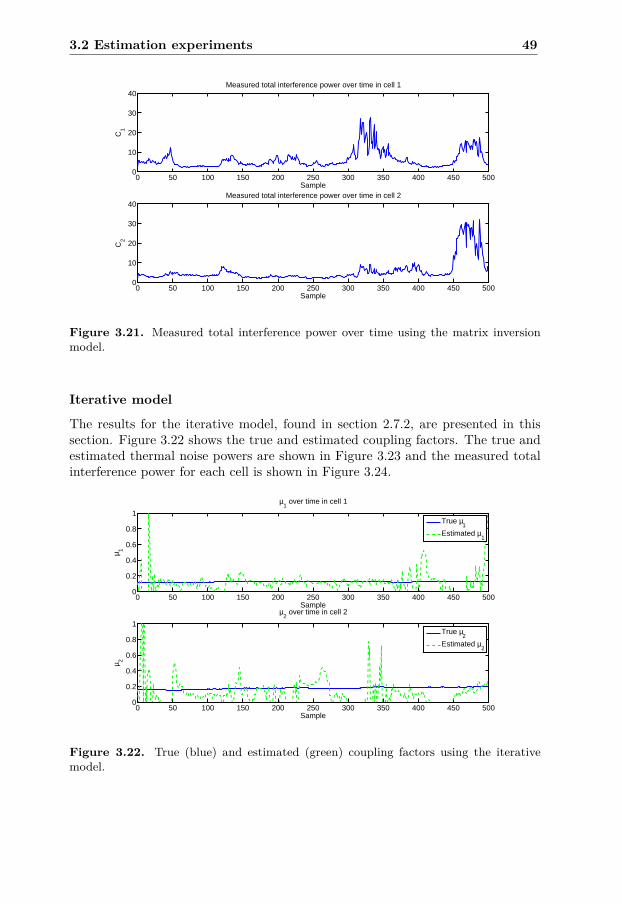
Figure 3.21. Measured total interference power over time using the matrix inversionmodel.
Iterative model
The results for the iterative model, found in section 2.7.2, are presented in thissection. Figure 3.22 shows the true and estimated coupling factors. The true andestimated thermal noise powers are shown in Figure 3.23 and the measured totalinterference power for each cell is shown in Figure 3.24.
0 50 100 150 200 250 300 350 400 450 5000
0.2
0.4
0.6
0.8
1
Sample
µ 1
µ1 over time in cell 1
True µ
1
Estimated µ1
0 50 100 150 200 250 300 350 400 450 5000
0.2
0.4
0.6
0.8
1
Sample
µ 2
µ2 over time in cell 2
True µ
2
Estimated µ2
Figure 3.22. True (blue) and estimated (green) coupling factors using the iterativemodel.

50 Results
0 50 100 150 200 250 300 350 400 450 5000
1
2
3
4
N01
over time in cell 1
Sample
N01
0 50 100 150 200 250 300 350 400 450 5000
10
20
30
40
N02
over time in cell 2
Sample
N02
True N01
Estimated N01
True N02
Estimated N02
Figure 3.23. True (blue) and estimated (green) thermal noise power using the iterativemodel.
0 50 100 150 200 250 300 350 400 450 5000
10
20
30Measured total interference power over time in cell 1
Sample
C1
0 50 100 150 200 250 300 350 400 450 5000
10
20
30Measured total interference power over time in cell 2
Sample
C2
Figure 3.24. Measured total interference power over time using the iterative model.
3.2 Estimation experiments 51
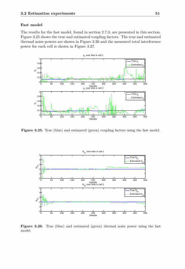
Fast model
The results for the fast model, found in section 2.7.3, are presented in this section.Figure 3.25 shows the true and estimated coupling factors. The true and estimatedthermal noise powers are shown in Figure 3.26 and the measured total interferencepower for each cell is shown in Figure 3.27.
0 50 100 150 200 250 300 350 400 450 5000
0.2
0.4
0.6
0.8
1
Sample
µ 1
µ1 over time in cell 1
True µ
1
Estimated µ1
0 50 100 150 200 250 300 350 400 450 5000
0.2
0.4
0.6
0.8
1
Sample
µ 2
µ2 over time in cell 2
True µ
2
Estimated µ2
Figure 3.25. True (blue) and estimated (green) coupling factors using the fast model.
0 50 100 150 200 250 300 350 400 450 5000
1
2
3
4
5
N01
over time in cell 1
Sample
N01
0 50 100 150 200 250 300 350 400 450 5000
1
2
3
4
5
N02
over time in cell 2
Sample
N02
True N01
Estimated N01
True N02
Estimated N02
Figure 3.26. True (blue) and estimated (green) thermal noise power using the fastmodel.

52 Results
0 50 100 150 200 250 300 350 400 450 5000
10
20
30Measured total interference power over time in cell 1
Sample
C1
0 50 100 150 200 250 300 350 400 450 5000
10
20
30Measured total interference power over time in cell 2
Sample
C2
Figure 3.27. Measured total interference power over time using the fast model.
Model with fixed λ
The results for the model with fixed λ, found in section 2.7.4, are presented in thissection. Figure 3.28 shows the true and estimated coupling factors. The true andestimated thermal noise powers are shown in Figure 3.29 and the measured totalinterference power for each cell is shown in Figure 3.30.
0 50 100 150 200 250 300 350 400 450 5000
0.2
0.4
0.6
0.8
1
Sample
µ 1
µ1 over time in cell 1
True µ
1
Estimated µ1
0 50 100 150 200 250 300 350 400 450 5000
0.2
0.4
0.6
0.8
1
Sample
µ 2
µ2 over time in cell 2
True µ
2
Estimated µ2
Figure 3.28. True (blue) and estimated (green) coupling factors using the model withfixed λ.

3.2 Estimation experiments 53
0 50 100 150 200 250 300 350 400 450 5000
5
10
15
N01
over time in cell 1
Sample
N01
0 50 100 150 200 250 300 350 400 450 5000
5
10
15
N02
over time in cell 2
Sample
N02
True N01
Estimated N01
True N02
Estimated N02
Figure 3.29. True (blue) and estimated (green) thermal noise power using the modelwith fixed λ.
0 50 100 150 200 250 300 350 400 450 5000
10
20
30Measured total interference power over time in cell 1
Sample
C1
0 50 100 150 200 250 300 350 400 450 5000
10
20
30Measured total interference power over time in cell 2
Sample
C2
Figure 3.30. Measured total interference power over time using the fast model.

54 Results
Conclusions
By examining the estimates and measurements made using the four different in-terference models the following conclusions can be made
• Matrix inversion model - the estimated states are close to the true statesand are not especially noisy. By comparing the result in Figures 3.19-3.21to those in section 3.2.2 it can be seen that the quality of the estimates hasbeen reduced. The reason for this is that things are not as ideal as beforesince the noise on µ1 and µ2 is no longer known.
• Iterative model - the estimated states are noisy and do not follow the truestates as well as the ones calculated using the matrix inversion model. Bycomparing Figure 3.21 and Figure 3.24 it can be seen that this model hastrouble handling fast variations. This is probably the reason for the reducedquality of the estimates.
• Fast model - just like before the estimated states are noisy but correct inthe mean. By looking more closely at the measured total interference powerit can be seen that the reaction from this model is delayed by a few samplescompared to the matrix inversion model. It does however react faster thanthe iterative model.
• Model using λ - the estimates calculated using this model are less noisythan the results from the iterative- and fast model. The estimates for thismodel are made using λ = 0.1 which makes the model react even faster thanthe fast model.
The Matrix inversion model is preferred due to the fact that it has an instantresponse to changes, a property that seems to improve the the quality of theestimates.

3.2 Estimation experiments 55
3.2.4 Experiment DThe purpose of this experiment is to make the setup further resemble the realsituation. This is done by adding noise to the measurements entering the Kalmanfilter. Note that there is still no noise on the measurements passed to the C-matrix. The setup for this experiment is shown in Figure 3.31 and the randomwalks of the two UEs are shown in Figure 3.32.
KF
y(k)
x̂(k)
z−1
M1Sim
l(k)
µ(k)
sat(·)ˆ̂x(k)
C
v(k)
++
Figure 3.31. Block diagram of the experiment.
−400 −200 0 200 400 600 800 1000 1200 1400
−400
−300
−200
−100
0
100
200
300
400Cell 1 Cell 2
UE positions
Distance x [m]
Dis
tanc
e y
[m]
Figure 3.32. Random walk of the UE in each cell.
Compared to the previous experiments the measurements now contain more noise.In order to put less trust into the noisy measurements theR-matrix is made larger.The values have been found through trial and error.
R =[1e-3 0
0 1e-3
]

56 Results
The results for this setup are shown in Figure 3.33, 3.34, 3.35 and 3.36.
0 50 100 150 200 250 300 350 400 450 5000
0.2
0.4
0.6
0.8
1Load over time in cell 1
Sample
Load
0 50 100 150 200 250 300 350 400 450 5000
0.2
0.4
0.6
0.8
1Load over time in cell 2
Sample
Load
Figure 3.33. Loads over time in the two cells. The total loads are shown in black andthe loads of the UEs are shown in blue.
0 50 100 150 200 250 300 350 400 450 5000
0.5
1
Sample
µ 1
µ1 over time in cell 1
True µ
1
Estimated µ1
0 50 100 150 200 250 300 350 400 450 5000
0.5
1
Sample
µ 2
µ2 over time in cell 2
True µ
2
Estimated µ2
Figure 3.34. True (blue) and estimated (green) coupling factors using the matrix in-version model.

3.2 Estimation experiments 57
0 50 100 150 200 250 300 350 400 450 5000
2
4
6
N01
over time in cell 1
Sample
N01
True N
01
Estimated N01
0 50 100 150 200 250 300 350 400 450 5000
5000
10000
N02
over time in cell 2
Sample
N02
True N
02
Estimated N02
Figure 3.35. True (blue) and estimated (green) thermal noise power using the matrixinversion model.
0 50 100 150 200 250 300 350 400 450 5000
5
10
15Measured total interference power over time in cell 1
Sample
C1
0 50 100 150 200 250 300 350 400 450 5000
5
10
15Measured total interference power over time in cell 2
Sample
C2
Figure 3.36. Measured total interference power over time using the matrix inversionmodel.
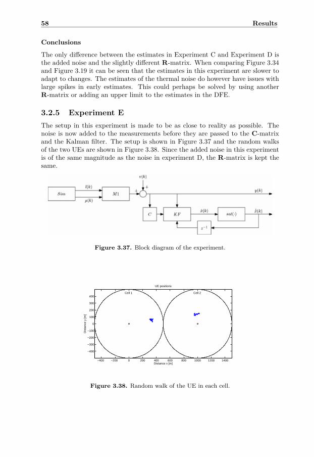
58 Results
Conclusions
The only difference between the estimates in Experiment C and Experiment D isthe added noise and the slightly different R-matrix. When comparing Figure 3.34and Figure 3.19 it can be seen that the estimates in this experiment are slower toadapt to changes. The estimates of the thermal noise do however have issues withlarge spikes in early estimates. This could perhaps be solved by using anotherR-matrix or adding an upper limit to the estimates in the DFE.
3.2.5 Experiment EThe setup in this experiment is made to be as close to reality as possible. Thenoise is now added to the measurements before they are passed to the C-matrixand the Kalman filter. The setup is shown in Figure 3.37 and the random walksof the two UEs are shown in Figure 3.38. Since the added noise in this experimentis of the same magnitude as the noise in experiment D, the R-matrix is kept thesame.
Figure 3.37. Block diagram of the experiment.
−400 −200 0 200 400 600 800 1000 1200 1400
−400
−300
−200
−100
0
100
200
300
400Cell 1 Cell 2
UE positions
Distance x [m]
Dis
tanc
e y
[m]
Figure 3.38. Random walk of the UE in each cell.

3.2 Estimation experiments 59
The results for this setup are shown in Figure 3.39, 3.40, 3.41 and 3.42.
0 50 100 150 200 250 300 350 400 450 5000
0.2
0.4
0.6
0.8
1Load over time in cell 1
Sample
Load
0 50 100 150 200 250 300 350 400 450 5000
0.2
0.4
0.6
0.8
1Load over time in cell 2
Sample
Load
Figure 3.39. Loads over time in the two cells. The total loads are shown in black andthe loads of the UEs are shown in blue.
0 50 100 150 200 250 300 350 400 450 5000
0.5
1
Sample
µ 1
µ1 over time in cell 1
True µ
1
Estimated µ1
0 50 100 150 200 250 300 350 400 450 5000
0.5
1
Sample
µ 2
µ2 over time in cell 2
True µ
2
Estimated µ2
Figure 3.40. True (blue) and estimated (green) coupling factors using the matrix in-version model.

60 Results
0 50 100 150 200 250 300 350 400 450 5000
5
10
15
20
N01
over time in cell 1
Sample
N01
True N
01
Estimated N01
0 50 100 150 200 250 300 350 400 450 5000
5
10x 10
11 N02
over time in cell 2
Sample
N02
True N
02
Estimated N02
Figure 3.41. True (blue) and estimated (green) thermal noise power using the matrixinversion model.
0 50 100 150 200 250 300 350 400 450 5000
5
10
15
20Measured total interference power over time in cell 1
Sample
C1
0 50 100 150 200 250 300 350 400 450 5000
5
10
15
20Measured total interference power over time in cell 2
Sample
C2
Figure 3.42. Measured total interference power over time using the matrix inversionmodel.
Conclusions
By comparing the results in Figure 3.40 and Figure 3.34 it can be seen that thequality of the estimates is noticeably worse. The reason for this is that the noiseis now also passed to the C-matrix. As in the previous experiment the estimatesof the thermal noise have issues with large spikes in early estimates.

Chapter 4
Concluding remarks
This chapter contains a summary of the most important conclusions and resultsin this thesis. It also contains some remarks regarding what can be studied in thefuture.
4.1 ConclusionsThe purpose of this thesis is to better understand single cell and multi-cell interfer-ence in 3G mobile communication systems. The problem of inter-cell interferencehas been studied from a new angle and some interesting conclusions have beendrawn. This has been done by gradually satisfying the goals described in sec-tion 1.1.
The stability experiments described in section 3.1 show some interesting resultsregarding the highest achievable data-rate in a cell, after expanding the model toinclude contributions from neighboring cells. They show that the position of theUE has a significant impact on both mean and variance of the highest achievablegrant. It is also shown that reducing the grant of the users or increasing the num-ber of users lowers the variance.
The next interesting conclusion can be found in section 2.3. There it is shownthat the commonly used rule of thumb for stability using loads, which is basedon the result for an isolated cell, is not very safe when contributions from othercells are taken into account. Section 2.4 provides a new sufficient condition forstability that takes neighboring cells into account. It also contains a necessary andsufficient condition for the two-cell case.
61

62 Concluding remarks
In section 2.5 it is shown that a less conservative version of the sufficient conditionmentioned above can be used. This requires knowledge of the coupling factors fromone cell to another, which need to be estimated. Section 3.2 shows the results ofusing a quasi-decentralized estimation strategy to estimate this parameter. It isconcluded that the estimates can be improved by adding a DFE. It can be seenthat the quasi-decentralized approach using a Kalman filter works quite well ina fairly ideal environment but that it has problems once noise is added to themeasurements. Since the model is nonlinear the estimates could probably beimproved by using a nonlinear filtering method such as the Extended Kalmanfilter or a Particle filter.
4.2 Future workThis thesis is an introduction to the communication problem known as inter-cellinterference. There is still a lot of research to be done in this area. As mentionedin section 4.1, a nonlinear filter may be considered for the estimate of the couplingfactors. Furthermore, dividing the users in a cell into different classes such as weakand strong users may also improve the estimate.
Additional complications that are not considered in this thesis that may be inter-esting to explore include but are not limited to: users entering and leaving thecells, users in soft handover, fading, cell coverage etc.
Another thing to look into is how a model can be developed to determine theloads allowed in each cell given the estimate of the coupling factors. Such a modelcould then be used by a scheduler to distribute new grants whilst maintaining cellstability.

Bibliography
[1] Sheng Chen, Bernard Mulgrew, and Stephen McLaughlin. Adaptive BayesianEqualizer with Decision Feedback. IEEE Transactions On Signal Processing,1993.
[2] Erik Dahlman, Stefan Parkvall, Johan Sköld, and Per Beming. 3G Evolution,HSPA and LTE for Mobile Broadband. Academic Press, 1st edition, 2007.ISBN 9-780-12372-5332.
[3] Claude E. Shannon. Communications in the Presence of Noise. Proceedingsof the IEEE, 1998.
[4] Torkel Glad and Lennart Ljung. Reglerteori: Flervariabla och olinjärametoder. Studentlitteratur, 2nd edition, 2003. ISBN 9-789-14403-0036.
[5] Fredrik Gustafsson. Particle Filter Theory and Practice with PositioningApplications. IEEE Aerospace And Electronic Systems Magazine, 2010.
[6] Fredrik Gustafsson. Statistical Sensor Fusion. Studentlitteratur, 1st edition,2010. ISBN 9-789-14405-4896.
[7] Fredrik Gustafsson and Fredrik Gunnarsson. Control theory aspects of powercontrol in UMTS. Control Engineering Practice, 2003.
[8] Harri Holma and Antti Toskala. WCDMA for UMTS-Radio Access For ThirdGeneration Mobile Communications. John Wiley & Sons, 2nd edition, 2002.ISBN 0-470-84467-1.
[9] Katrina Lau, Graham Goodwin, Mauricio Cea, and Torbjörn Wigren. Lin-ear and Nonlinear Decoupling for Inner Loop Power Control in 3G MobileCommunications. To be presented at the 18th IFAC World Congress, 2011.
[10] Lennart Ljung and Torkel Glad. Modellbygge och Simulering. Studentlitter-atur, 1st edition, 2004. ISBN 9-789-14402-4431.
[11] Pillai S. Unnikrishna, Torsten Suel, and Seunghun Cha. The Perron-Frobenius theorem. IEEE Signal Processing Magazine, 2005.
[12] Torbjörn Wigren. Soft Uplink Load Estimation in WCDMA. IEEE Transac-tions On Vehicular Technology, 2009.
63

64 Bibliography
[13] Torbjörn Wigren. Recursive Noise Floor Estimation in WCDMA. IEEETransactions On Vehicular Technology, 2010.
[14] Torbjörn Wigren and Per Hellqvist. Estimation of uplink WCDMA load in asingle RBS. IEEE Transactions On Vehicular Technology, 2007.

Appendix A
Abbreviations
2G Second Generation Communication System3G Third Generation Communication SystemBLUE Best Linear Unbiased EstimatorDFE Decision Feedback EqualizerKF Kalman FilterLTE Long Term EvolutionMIMO Multiple-Input Multiple-OutputMPF Marginalized Particle FilterNMT Nordic Mobile TelephonyPDF Probability Density FunctionPF Particle FilterRBS Radio Base StationRTWP Received Total Wideband PowerSIR Signal-to-Interference RatioSISO Single-Input Single-OutputSMS Short Message ServiceSNR Signal-to-Noise RatioUE User EquipmentUMTS Universal Mobile Telecommunication SystemWCDMA Wideband Code Division Multiple Access
65

Appendix B
Notation
A bar¯is used to denote linear quantities.
α Self-interference constantβ Bandwidth utilizationε Load thresholdγ Power grantλ Eigenvalue, also used to denote a forgetting factor
in one of the interference modelsφ0 Constant noise power spectral densityρ Scaling factor, also used to denote the spectral
radius in the Perron-Frobenius theoremµ Coupling factor for a cell, also used to denote
mean valueσ Standard deviationBW BandwidthC Total interference powerEb Energy received per bitg Fading gainI Interference powerIother Interference power from users in other cellsIC Coupling factor for a userL Load generated by a userN NoiseN0 Thermal noiseP Received signal powerp Received powerp′ Transmitted power
66

67
R Rate of data communicationT Channel capacityS Signal-to-Interference RatioS∗ Desired Signal-to-Interference Ratio

Appendix C
Matlab code for theestimation experiments
1 function estimation(mu_method,I_model,sim,DFE,dl,g,samples,...2 Q,R,P0,du,lambda)3
4 % ####################################################################### %5 % Description:6 % Runs a Kalman filter estimation experiment.7 %8 % Input:9 % mu_method − determines which method is used to generate mu.
10 % 1 − use model11 % 2 − simulate a random walk in the cell12 % I_model − determines which model is used to create the measurements13 % 1 − Matrix inversion model14 % 2 − Iterative model15 % 3 − Quick model16 % 4 − Lambda model17 % 5 − Use and produce results for all the models18 % sim − determines if and how noise is added to the measurements19 % 1 − No noise20 % 2 − Noise added between the C−Matrix and the Kalman filter21 % 3 − Noise added before the C−Matrix and the Kalman filter22 % DFE − determines if DFE should be used or not23 % 1 or true − Use DFE24 % 0 or false − Do not use DFE25 % dl − standard deviation of the loads26 % g − a 1−dim vector containing two values of rho to be used in the27 % A−matrix28 % samples − how many samples to produce29 % Q − Process noise covariance matrix 4x430 % R − Measurement noise covariance matrix 2x231 % P0 − Initial covariance matrix 4x432 % du− standard deviation of the movement speed of the user in m/sample33 % (Only used by mu_method 2)34 % lambda − the forgetting factor used in the lambda model (Used together
68

69
35 % with I_model 4)36 %37
38 %################################################################%39 % Make sure all the plots are formatted to be used in the report %40 %################################################################%41 plotfix(0)42
43 %####################%44 % Initiate variables %45 %####################%46 if nargin < 11,47 du = 0;48 lambda = 0;49 end50
51 % Simulation variables52 R1 = 500;53 R2 = 500;54 distB1B2 = R1+R2; % distance from base station 1 to base station 255 % (no overlap and no gap)56 dirB1B2 = [1 0]; % direction from base station 1 to base station 257 B1B2 = distB1B2*dirB1B2;58
59 % Plot data and measurements60 xpos1 = zeros(1,samples); % x positions of the users in cell 161 ypos1 = zeros(1,samples); % y positions of the users in cell 162 xpos2 = zeros(1,samples); % x positions of the users in cell 263 ypos2 = zeros(1,samples); % y positions of the users in cell 264 mu1 = zeros(1,samples);65 mu2 = zeros(1,samples);66 loads1 = zeros(1,samples);67 loads2 = zeros(1,samples);68
69 % Constants70 noise_floor = 10^(−107/10)/10^3; % dBm −> W71
72 % Kalman filter73 x0 = [0.2; 0.2; noise_floor*10^14; noise_floor*10^14];74 A = [g(1) 0 0 075 0 g(2) 0 076 0 0 1 077 0 0 0 1];78
79 %############%80 % Generate $\mu$ %81 %############%82 switch mu_method,83 case 1,84 x_gen = zeros(4,samples);85 x_gen(:,1) = x0;86 h_wait = waitbar(1/samples,sprintf(['Generating $\mu$\nProgress\n' ...87 num2str(round(1/samples*100)) '%%']));88 for k = 2:samples,89 x_new = A*x_gen(:,k−1)+sqrt(Q)*randn(4,1);90 x_gen(:,k) = dfe_check(x_new);91 waitbar(k/samples,h_wait,sprintf(['Generating $\mu$\nProgress\n' ...92 num2str(round(k/samples*100)) '%%']))

70 Matlab code for the estimation experiments
93 end94 close(h_wait)95 mu1 = x_gen(1,:);96 mu2 = x_gen(2,:);97 case 2,98 d1 = zeros(1,samples);99 d12 = zeros(1,samples);
100 d2 = zeros(1,samples);101 d21 = zeros(1,samples);102
103 % Place user in cell 1104 inside = false;105 while ~inside,106 x = randi([−R1,R1],1);107 y = randi([−R1,R1],1);108
109 if sqrt(x^2+y^2) <= R1,110 % Save position and calculate distances111 xpos1(1) = x;112 ypos1(1) = y;113 d1(1) = norm([x y]);114 d12(1) = norm(B1B2−[x y]);115
116 % Increment117 inside = true;118 end119 end120
121 % Place user in cell 2122 inside = false;123 while ~inside,124 x = randi([−R2,R2],1);125 y = randi([−R2,R2],1);126
127 if sqrt(x^2+y^2) <= R2,128 % Save position and calculate distances129 xpos2(1) = B1B2(1)+x;130 ypos2(1) = B1B2(2)+y;131 d2(1) = norm([x y]);132 d21(1) = norm(−B1B2−[x y]);133
134 % Increment135 inside = true;136 end137 end138
139 % Random walk the users140 h_wait = waitbar(1/samples,sprintf(['Generating $\mu$\nProgress\n' ...141 num2str(round(1/samples*100)) '%%']));142 for k = 2:samples,143 inside = false;144 while ~inside,145 x = xpos1(k−1)+du*randn;146 y = ypos1(k−1)+du*randn;147
148 if norm([x y]) <= R1,149 % Save position and calculate distances150 xpos1(k) = x;

71
151 ypos1(k) = y;152 d1(k) = norm([x y]);153 d12(k) = norm(B1B2−[x y]);154
155 % Increment156 inside = true;157 end158 end159
160 inside = false;161 while ~inside,162 x = xpos2(k−1)+du*randn;163 y = ypos2(k−1)+du*randn;164
165 if norm([x y]−B1B2) <= R2,166 % Save position and calculate distances167 xpos2(k) = x;168 ypos2(k) = y;169 d2(k) = norm([x y]−B1B2);170 d21(k) = norm([x y]);171
172 % Increment173 inside = true;174 end175 end176 waitbar(k/samples,h_wait,...177 sprintf(['Generating $\mu$\nProgress\n' ...178 num2str(round(k/samples*100)) '%%']))179 end180 close(h_wait)181
182 mu1 = (d1./d12).^2;183 mu2 = (d2./d21).^2;184 end185
186 %################%187 % Generate loads %188 %################%189 loads1(1) = 1/2;190 loads2(1) = 1/2;191
192 h_wait = waitbar(1/samples,sprintf(['Generating loads\nProgress\n' ...193 num2str(round(1/samples*100)) '%%']));194 for k = 2:samples,195 loads1(k) = loads1(k−1) + dl*randn;196 if loads1(k) < 0,197 loads1(k) = 0;198 elseif loads1(k) > 0.8,199 loads1(k) = 0.8;200 end201
202 loads2(k) = loads2(k−1) + dl*randn;203 if loads2(k) < 0,204 loads2(k) = 0;205 elseif loads2(k) > 0.8,206 loads2(k) = 0.8;207 end208
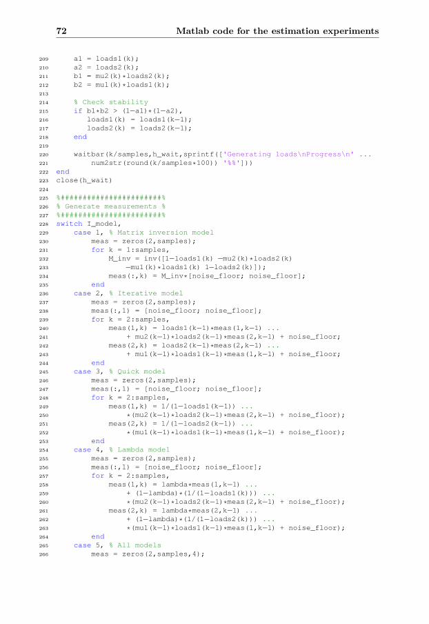
72 Matlab code for the estimation experiments
209 a1 = loads1(k);210 a2 = loads2(k);211 b1 = mu2(k)*loads2(k);212 b2 = mu1(k)*loads1(k);213
214 % Check stability215 if b1*b2 > (1−a1)*(1−a2),216 loads1(k) = loads1(k−1);217 loads2(k) = loads2(k−1);218 end219
220 waitbar(k/samples,h_wait,sprintf(['Generating loads\nProgress\n' ...221 num2str(round(k/samples*100)) '%%']))222 end223 close(h_wait)224
225 %#######################%226 % Generate measurements %227 %#######################%228 switch I_model,229 case 1, % Matrix inversion model230 meas = zeros(2,samples);231 for k = 1:samples,232 M_inv = inv([1−loads1(k) −mu2(k)*loads2(k)233 −mu1(k)*loads1(k) 1−loads2(k)]);234 meas(:,k) = M_inv*[noise_floor; noise_floor];235 end236 case 2, % Iterative model237 meas = zeros(2,samples);238 meas(:,1) = [noise_floor; noise_floor];239 for k = 2:samples,240 meas(1,k) = loads1(k−1)*meas(1,k−1) ...241 + mu2(k−1)*loads2(k−1)*meas(2,k−1) + noise_floor;242 meas(2,k) = loads2(k−1)*meas(2,k−1) ...243 + mu1(k−1)*loads1(k−1)*meas(1,k−1) + noise_floor;244 end245 case 3, % Quick model246 meas = zeros(2,samples);247 meas(:,1) = [noise_floor; noise_floor];248 for k = 2:samples,249 meas(1,k) = 1/(1−loads1(k−1)) ...250 *(mu2(k−1)*loads2(k−1)*meas(2,k−1) + noise_floor);251 meas(2,k) = 1/(1−loads2(k−1)) ...252 *(mu1(k−1)*loads1(k−1)*meas(1,k−1) + noise_floor);253 end254 case 4, % Lambda model255 meas = zeros(2,samples);256 meas(:,1) = [noise_floor; noise_floor];257 for k = 2:samples,258 meas(1,k) = lambda*meas(1,k−1) ...259 + (1−lambda)*(1/(1−loads1(k))) ...260 *(mu2(k−1)*loads2(k−1)*meas(2,k−1) + noise_floor);261 meas(2,k) = lambda*meas(2,k−1) ...262 + (1−lambda)*(1/(1−loads2(k))) ...263 *(mu1(k−1)*loads1(k−1)*meas(1,k−1) + noise_floor);264 end265 case 5, % All models266 meas = zeros(2,samples,4);

73
267 meas(:,1,1) = [noise_floor; noise_floor];268 meas(:,1,2) = [noise_floor; noise_floor];269 meas(:,1,3) = [noise_floor; noise_floor];270 meas(:,1,4) = [noise_floor; noise_floor];271
272 for k = 2:samples,273 % Matrix inversion model274 M_inv = inv([1−loads1(k) −mu2(k)*loads2(k)275 −mu1(k)*loads1(k) 1−loads2(k)]);276 meas(:,k,1) = M_inv*[noise_floor; noise_floor];277
278 % Iterative model279 meas(1,k,2) = loads1(k−1)*meas(1,k−1,2) ...280 + mu2(k−1)*loads2(k−1)*meas(2,k−1,2) + noise_floor;281 meas(2,k,2) = loads2(k−1)*meas(2,k−1,2) ...282 + mu1(k−1)*loads1(k−1)*meas(1,k−1,2) + noise_floor;283
284 % Quick model285 meas(1,k,3) = 1/(1−loads1(k−1)) ...286 *(mu2(k−1)*loads2(k−1)*meas(2,k−1,3) + noise_floor);287 meas(2,k,3) = 1/(1−loads2(k−1)) ...288 *(mu1(k−1)*loads1(k−1)*meas(1,k−1,3) + noise_floor);289
290 % Lambda model291 meas(1,k,4) = lambda*meas(1,k−1,4) ...292 + (1−lambda)*(1/(1−loads1(k)))...293 *(mu2(k−1)*loads2(k−1)*meas(2,k−1,4) + noise_floor);294 meas(2,k,4) = lambda*meas(2,k−1,4) ...295 + (1−lambda)*(1/(1−loads2(k))) ...296 *(mu1(k−1)*loads1(k−1)*meas(1,k−1,4) + noise_floor);297 end298 end299
300 %###########%301 % Add noise %302 %###########%303 % NOTE: y1 is the measurement vector passed to the C−matrix and y2 is the304 % measurement vector passed to the Kalman filter.305 noise_std = 0.1*noise_floor;306 switch sim,307 case 1,308 y1 = meas;309 y2 = meas;310 case 2,311 y1 = meas;312 if ndims(meas) == 2,313 y2 = meas + noise_std*randn(2,samples);314 else315 y2 = meas + noise_std*randn(2,samples,4);316 end317 case 3,318 if ndims(meas) == 2,319 y1 = meas + noise_std*randn(2,samples);320 y2 = y1;321 else322 y1 = meas + noise_std*randn(2,samples,4);323 y2 = y1;324 end

74 Matlab code for the estimation experiments
325 end326
327 %############%328 % Run filter %329 %############%330 if I_model == 5,331 models = 4;332 else333 models = 1;334 end335
336 % Rescale the measurements337 y1 = y1*10^14;338 y2 = y2*10^14;339
340 % Create the storage variable x_hat341 x_hat = zeros(4,samples,models);342
343 for i = 1:models,344 % Initiate the estimation345 x_hat(:,1,i) = [mu1(1); mu2(1); noise_floor*10^14; noise_floor*10^14];346
347 % Create the second estimate to initiate the Kalman filter gain348 P = P0;349 C = [0 loads2(1)*y1(2,1,i)/(1−loads1(1)) 1/(1−loads1(1)) 0350 loads1(1)*y1(1,1,i)/(1−loads2(1)) 0 0 1/(1−loads2(1))];351 S=inv(C*P*C'+R);352 K=A*P*C'*S;353
354 x_hat(:,2,i) = A*x_hat(:,1,i)+K*(y2(:,1,i)−C*x_hat(:,1,i));355
356 % If selected, run DFE357 if DFE,358 x_hat(:,2,i) = dfe_check(x_hat(:,2,i));359 end360
361 for k = 2:samples−1,362 % Compute new output matrix363 C = [0 loads2(k)*y1(2,k,i)/(1−loads1(k)) 1/(1−loads1(k)) 0364 loads1(k)*y1(1,k,i)/(1−loads2(k)) 0 0 1/(1−loads2(k))];365
366 % If sim == 2 or 3 run, update the R−matrix367 % if sim == 2 || sim == 3,368 % R = R;369 % end370
371 % Compute the Kalman filter gain372 P=A*P*A'+Q−A*P*C'*S*C*P*A';373 S=inv(C*P*C'+R);374 K=A*P*C'*S;375
376 % Estimate the next state vector377 x_hat(:,k+1,i) = A*x_hat(:,k,i)+K*(y2(:,k,i)−C*x_hat(:,k,i));378
379 % If selected, run DFE380 if DFE,381 x_hat(:,k+1,i) = dfe_check(x_hat(:,k+1,i));382 end

75
383 end384 end385
386 %##############%387 % Plot results %388 %##############%389
390 % Plot UE walk391 if mu_method == 2,392 figure393 plot(0,0,'ko',B1B2(1),B1B2(2),'ko')394 hold on395 plot(xpos1,ypos1,'b−',xpos1(1),ypos1(1),'bo',...396 xpos1(end),ypos1(end),'b*')397 plot(xpos2,ypos2,'b−',xpos2(1),ypos2(1),'bo',...398 xpos2(end),ypos2(end),'b*')399 circle([0,0],R1,1000,'k−');400 circle(B1B2,R2,1000,'k−');401 text(−60,R1−50,'Cell 1')402 text(B1B2(1)−60,B1B2(2)+R2−50,'Cell 2')403 title('UE positions')404 xlabel('Distance x [m]')405 ylabel('Distance y [m]')406 hold off407 axis image408 end409
410 % Plot the loads411 figure412 subplot(2,1,1)413 total1 = loads1 + mu2.*loads2;414 plot(0:samples−1,loads1,'b−',0:samples−1,total1,'k−')415 title('Load over time in cell 1')416 xlabel('Sample')417 ylabel('Load')418
419 subplot(2,1,2)420 total2 = loads2 + mu1.*loads1;421 plot(0:samples−1,loads2,'b−',0:samples−1,total2,'k−')422 title('Load over time in cell 2')423 xlabel('Sample')424 ylabel('Load')425
426 % Plot estimations and measurements427 for i = 1:models,428 % Plot mu429 figure430 subplot(2,1,1)431 plot(0:samples−1,mu1,'b−',0:samples−1,x_hat(1,:,i),'g−−')432 legend('True $\mu$_1', 'Estimated $\mu$_1')433 title('$\mu$_1 over time in cell 1')434 xlabel('Sample')435 ylabel('$\mu$_1')436
437 subplot(2,1,2)438 plot(0:samples−1,mu2,'b−',0:samples−1,x_hat(2,:,i),'g−−')439 legend('True $\mu$_2', 'Estimated $\mu$_2')440 title('$\mu$_2 over time in cell 2')

76 Matlab code for the estimation experiments
441 xlabel('Sample')442 ylabel('$\mu$_2')443
444 % Plot thermal noise power445 figure446 subplot(2,1,1)447 plot(0:samples−1,10^14*noise_floor*ones(samples,1),'b−',...448 0:samples−1,x_hat(3,:,i),'g−−')449 title('N_{01} over time in cell 1')450 xlabel('Sample')451 ylabel('N_{01}')452 legend('True N_{01}', 'Estimated N_{01}')453
454 subplot(2,1,2)455 plot(0:samples−1,10^14*noise_floor*ones(samples,1),'b−',...456 0:samples−1,x_hat(4,:,i),'g−−')457 title('N_{02} over time in cell 2')458 xlabel('Sample')459 ylabel('N_{02}')460 legend('True N_{02}', 'Estimated N_{02}')461
462 % Plot total interference power463 figure464 subplot(2,1,1)465 plot(0:samples−1,y2(1,:,i),'b−')466 title('Measured total interference power over time in cell 1')467 xlabel('Sample')468 ylabel('C_1')469
470 subplot(2,1,2)471 plot(0:samples−1,y2(2,:,i),'b−')472 title('Measured total interference power over time in cell 2')473 xlabel('Sample')474 ylabel('C_2')475 end

77
1 function sat_states = dfe_check(states)2
3 sat_states = states;4
5 if states(1)<0,6 sat_states(1) = 0;7 end8 if states(1)>1,9 sat_states(1) = 1;
10 end11 if states(2)<0,12 sat_states(2) = 0;13 end14 if states(2)>1,15 sat_states(2) = 1;16 end17 if states(3)<0,18 sat_states(3) = 0;19 end20 if states(4)<0,21 sat_states(4) = 0;22 end