ESTUDIOS DE ECONOMÍA APLICADA · Spearman rank correlation between actual and estimated efficiencies, ... is taken, which is an alternative measure of ... influence of wrongly considering

____________ Artículo recibido en noviembre de 2015 y aceptado en febrero de 2015 Artículo disponible en versión electrónica en la página www.revista-eea.net, ref. ә-33203 ISSN 1697-5731 (online) – ISSN 1133-3197 (print)

E S T U D I O S D E E C O N O M Í A A P L I C A D A

V O L . 33 - 2 2015

P Á G S . 619 – 632

On the Ability to Disentangle the Two Errors in the Normal/Half-Normal Stochastic Frontier Model

JOSE M. GAVILAN a, FRANCISCO J. ORTEGA a

a

Universidad de Sevilla, Facultad de CC.EE., Avda. Ramón y Cajal, 1, 41018 Sevilla, España. E-mail: [email protected], [email protected]

ABSTRACT In this paper, a simulation experiment is carried out in the framework of the normal/half-normal stochastic frontier model in order to analyse its ability to disentangle the two types of errors that form the composite error. According to the results obtained through the mean bias and the mean squared error of the parameters and efficiencies, and via Spearman rank correlation between actual and estimated efficiencies, a good performance of the model is only obtained when considering medium-sized or large samples and the variance of the inefficiencies highly contributes to that of the composite error. The problems of wrong skewness and absence of random error are also addressed. The influence on the results of selecting a wrong distribution for the inefficiency term is also analysed. Keywords: Production Models, Stochastic Frontier, Maximum Likelihood, Monte Carlo.

Sobre la capacidad de separar los dos errores en el modelo de frontera estocástica normal/half-normal

RESUMEN En este artículo, se lleva a cabo un experimento de simulación en el contexto del modelo con frontera estocástica normal/half-normal para analizar su capacidad de separar los dos tipos de error que forman el error compuesto. Según los resultados obtenidos a través del sesgo medio y el error cuadrático medio de los parámetros y las eficiencias, y mediante el coeficiente de correlación por rangos de Spearman entre las eficiencias reales y las estimadas, se obtiene un buen comportamiento del modelo solo cuando se consideran muestras de tamaño mediano o grande y la varianza de las ineficiencias contribuye de forma muy importante a la del error compuesto. Los problemas de la asimetría errónea y de la ausencia de errores aleatorios también son abordados. La influencia en los resultados de seleccionar una distribución errónea para el término de ineficiencia también se analiza. Palabras clave: Modelos de producción, frontera estocástica, máxima verosimilitud, Monte Carlo.

JEL Classification: C52, C63, C87

http://www.revista-eea.net/

mailto:[email protected]

mailto:[email protected]

JOSE M. GAVILAN Y FRANCISCO J. ORTEGA

Estudios de Economía Aplicada, 2015: 619-632 Vol. 33-2

620

1. INTRODUCTION The origins of the stochastic frontier production models (SFPM) are stated in

the seminal works of Aigner et al. (1977), Battese and Corra (1977), and Meeu-sen and van den Broeck (1977). This type of model is employed for the analysis of the efficiency of a production process in terms of the observed deviations between the actual production and the ideal frontier of maximum attainable output. In econometrics terms, such deviations can be identified through ran-dom perturbations in a regression model.

Ever since its appearance, this kind of model has been spread broadly across the scientific literature, and has been applied to a wide range of productive sec-tors. To mention a few of them, they have been extensively used in the produc-tive analysis in agriculture and fisheries (Battese and Broca, 1997; García et al., 2004), in the functioning of ports and airports (Barros, 2005, 2008), hospitals (O’Donnell and Nguyen, 2013), banking (Brissimis et al., 2010), and in the analysis of scientific production (Ortega and Gavilan, 2013).

The basic formulation of an SFPM is as follows:

( , ) u , 1,...,i i i iy f x v i nβ= + − = ,

where iy is the output or production of the i–th firm, ix the vector of all its inputs, β a vector of unknown parameters to estimate, and ( )f ⋅ the production function.

The random perturbation or error i i iv uε = − is composed of two parts (this is the reason why it is also known as a composed error model), a symmetrical random variable iv ∈ representing the random sources of variation and a one-sided random variable 0iu > designating the inefficiency of the produc-

tion process. Commonly, it is supposed that 2~ (0, ).i vv N σ With regard to the

inefficiency term iu , a positive probability distribution has to be chosen, since it measures the distance between the actual production and the stochastic fron-tier. In this paper, the most common hypothesis is analysed, that is, *

i iu u=

where * 2~ (0, ).i uu N σ By definition, it is said that the perturbations iu follow a

half-normal distribution, which is represented by 2~ (0, ).i uu HN σ Addi-tionally, it is supposed that the perturbations iv and iu are independent. With these selections, the model is known as the normal/half-normal stochastic frontier production model (Gómez-Gallego, Gómez-Gacía and Pérez-Cárceles, 2012; and Wang and Schmidt, 2009). It is important to mention that other types

ON THE ABILITY TO DISENTANGLE THE TWO ERRORS IN THE NORMAL/HALF-NORMAL…


621

of distributions for the perturbations iu have frequently been considered, inclu-ding the normal distribution truncated at a parameter µ not necessarily zero (Bhandari, 2011) and the exponential and gamma distributions, which have been widely used, especially when the Bayesian approach is assumed (Koop et al., 1995; Osiewalski and Steel, 1998; Koop and Steel, 2003).

In this paper, a Monte Carlo experiment is carried out to analyse the ability of the normal-half normal model to disentangle the two aforementioned types of error in order to provide good estimations of the parameters and efficiencies.

Taking into consideration the main objective of the paper, the choice of the functional form of the production function is not particularly significant, which is why the production function utilised is linear, that is, ( , ) 'i if x xβ β= ⋅ , whe-re the vector β has an intercept. Let us observe that, since ix and iy are mea-sured on a logarithmic scale, then the Cobb-Douglas production function is considered. In this most common case, instead of directly considering iu as the inefficiency measure, ( )exp iu− is taken, which is an alternative measure of efficiency with the additional advantage of being bounded between 0 and 1. For the sake of simplicity, the simulations are made on a model with an intercept and a single explanatory variable, since it has been proved that using a greater number of explanatory variables bears no effect on the results.

The maximum likelihood (ML) estimation of the SFPM has long been im-plemented by a range of statistical software, such as FRONTIER, LIMDEP, and STATA. Likewise, in the free and powerful statistical software R, several spe-cific packages can be found for this purpose. In this paper, the frontier package version 1.1-0 (Coelli and Henningsen, 2013) is utilised in order to obtain the ML estimators in the environment of the software R. This package uses the source code Fortran of the FRONTIER 4.1 software (Coelli, 1996).

Other studies, in which simulation analysis is carried out in SFPM, include: Coelli (1995), where the ML and the corrected least-squares estimators are compared; Zhang (1999), where the Bayesian estimation is set against the ML approach using a single point of the parametric space; and Ortega and Gavilan (2014), where a comparison between these two methodologies is carried out.

As a criterion for the comparison of the results, the mean squared error (MSE) is used in this paper, and special emphasis is placed on the parameter which indicates what proportion of the variance of the composite error is due to inefficiency, and on the estimation of the individual efficiencies.

This paper is organised as follows: in Section 2, the estimation of the model



622

and the design of the Monte Carlo experiment is described; in Section 3, the interpretation of the most interesting results is presented; Section 4 analyses the influence of wrongly considering a half-normal variable for the inefficiency term when the true distribution is gamma. Finally, in Section 5, the main con-clusions of this paper are drawn.

2. ESTIMATION OF THE MODEL AND DESIGN OF THE MONTE CARLO EXPERIMENT

The ML estimation of the SFPM is carried out by using the parameterisation by Battese and Corra (1977), where 2 2 2

v uσ σ σ= + and 2 2uγ σ σ= , which is

considered in the frontier package of the software R. Let us observe that γ is a parameter taking values between 0 and 1, and is an indicator of the proportion of the variance due to the inefficiency. It is important to point out that γ is not

exactly the proportion of the variances, since ( ) 2var uu pσ= , where

1 (2 / )p π= − . Specifically, if *γ is named as the proportion of the total variance due to inefficiency, (that is, ( ) ( ) ( )( )* var var varu u vγ = + ), then it is

straightforward to verify that ( )( )* 11 pγ γ γ γ −= + − .

With this parameterization, the logarithm of the likelihood for the i-th obser-vation is given by:

( )( )( )21 1log( ) log log( ) log 12 2 2i i iL z zπ σ γ γ = − − − + Φ − −

,

where '

i ii

y xz βσ−

= and ( )Φ ⋅ is the distribution function of a standard normal

random variable. Therefore, the ML estimation has to be obtained through nu-merical optimization algorithms.

With regard to the design of the Monte Carlo experiment, the sample space is given by 2 ,, ,nβ σ γ , and ix . By taking into consideration the invariance

results in Olson et al. (1980), the value of the parameter 2σ can be fixed. Therefore, 2 1σ = has been assumed. Without loss of generality, a single explanatory variable has been taken following a standard normal distribution (on logarithmic scale) and the parameter ( )0 1,β β β= (the intercept and the

slope) has been selected as ( ) ( )0 1, 1,0.3β β = (Zhang, 1999; Coelli, 1995).



623

The analysis performed in this paper is focused on the behaviour of the esti-mation of the parameter γ , along with the estimations of the individual efficiencies. One objective is to analyse the behaviour of the estimations as much in small samples as in medium-sized and large samples, which is why

{ }20,50,100,500n ∈ has been selected. With respect to the parameter *γ , the

values { }0,0.1,0.2,0.3,0.4,0.5,0.6,0.7,0.8,0.9,1 have been adopted. The corresponding values of the parameter γ are

*γ 0.0 0.1 0.2 0.3 0.4 0.5 0.6 0.7 0.8 0.9 1.0

γ 0.00 0.24 0.41 0.54 0.65 0.73 0.80 0.87 0.92 0.96 1.00

Therefore, eleven values of γ and four of n are simulated, which entails 44 combinations. For each combination, m 1000= replications of the model are made. In order to obtain the pseudorandom numbers, the generators imple-mented by default in R are used.

For each parameter, the mean bias (MB) and the mean squared error (MSE) observed in the m replications are calculated. With regard to the efficiencies, the MB, the MSE and the correlations1 between the actual and the estimated efficiencies are computed for each of the individual efficiencies. Afterwards, as a joint indicator, the averages are provided.

3. RESULTS OF THE MONTE CARLO EXPERIMENT The complete results of the Monte Carlo experiment, that is to say, the bias

and the MSE of all the parameters and the individual efficiencies and the Spearman correlations between the actual and estimated efficiencies in the 44 cases considered, are laid out in the Appendix. Here, the most relevant results are presented, while attention is focused on the MSE criterion, which indicates the performance of the considered model. The behaviour of the estimations of parameter γ and the individual efficiencies are our main concern. As already pointed out, parameter γ captures the structure of the composite error. It is cru-cial, in this type of model, to identify what proportion of the total error is due to inefficiency and what proportion is due to random effects. Therefore, the correct estimation of γ is extremely important for the attainment of the individual effi-ciencies of each firm, which constitutes one of the main objectives when using this kind of model.

In Figure 1, the estimations of the parameter γ for n=50 and the m=1000 replications of the model are represented for each value of γ* using histograms. The true value of γ is indicated by a vertical line. The model offers poor estima-

1 Spearman rank correlations are obtained. Pearson correlations are very similar.



624

tions for low values of the parameter although the performance of the estima-tions improves for large values of the parameter. This important conclusion is also reached for γ, the other parameters of the model and the efficiencies from Figure 2, where the MSEs of such quantities are shown for the considered values of n and γ*. As expected, the estimations improve as the sample size increases. Taking into consideration the different scales of the vertical axis, the model provides a less accurate estimate of the intercept 0β and of the variance

2σ than the other parameters and the efficiencies. The slope is estimated very accurately in all the cases.

Figure 1 Histograms of the parameter γ for n=50. The true value of γ is indicated as a vertical bar

Source: Own elaboration.

The similarity between the figures for the )(MSE γ and the (E )ffiMSE re-veals the direct influence that the estimation of the parameter γ exerts on the estimation of the efficiencies of the firms.

With regard to the biases (considered in absolute values), the same important conclusions can be drawn, since in general they decrease as γ and the sample size increase. In the same sense, the correlations between the actual and the



625

estimated efficiencies increase as γ and the sample size increase, and have values below 0.60 when .0 65γ ≤ for all the considered sample sizes.

Figure 2 MSEs of the parameters and efficiencies as a function of *γ and for the considered

sample sizes


In the analysis of the limitations of the model to disentangle the two types of errors in the model, it is important to study another problem: the tendency of the model to provide extreme estimations for the parameter γ , known as wrong skewness and absence of random errors.

The problem of wrong skewness (Waldman, 1982), appears when the residuals of the estimated model through ordinary least squares (OLS) have a positive coefficient of asymmetry, since the composite error of the model con-sidered in this paper has negative asymmetry (Green, 1993). In this case, it is obtained that ˆ 0γ = (no inefficiencies are present in the model) and the OLS and ML estimations of the model coincide. This problem is considered as an inconsistency of the model, and a change in the specification of the model or increase the sample size are recommended.



626

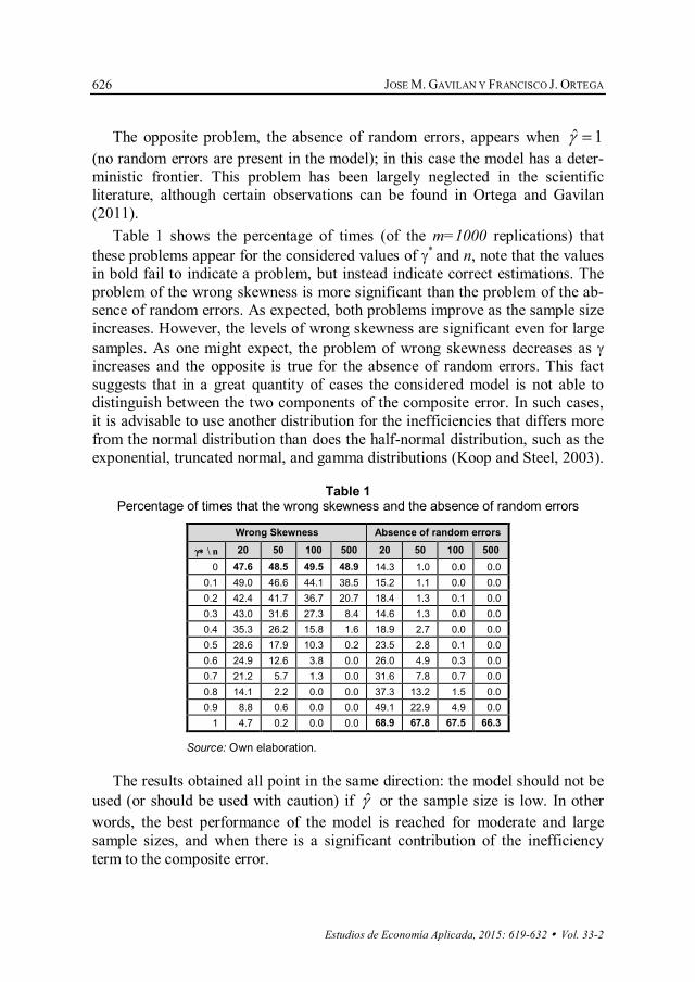
The opposite problem, the absence of random errors, appears when ˆ 1γ = (no random errors are present in the model); in this case the model has a deter-ministic frontier. This problem has been largely neglected in the scientific literature, although certain observations can be found in Ortega and Gavilan (2011).

Table 1 shows the percentage of times (of the m=1000 replications) that these problems appear for the considered values of γ* and n, note that the values in bold fail to indicate a problem, but instead indicate correct estimations. The problem of the wrong skewness is more significant than the problem of the ab-sence of random errors. As expected, both problems improve as the sample size increases. However, the levels of wrong skewness are significant even for large samples. As one might expect, the problem of wrong skewness decreases as γ increases and the opposite is true for the absence of random errors. This fact suggests that in a great quantity of cases the considered model is not able to distinguish between the two components of the composite error. In such cases, it is advisable to use another distribution for the inefficiencies that differs more from the normal distribution than does the half-normal distribution, such as the exponential, truncated normal, and gamma distributions (Koop and Steel, 2003).

Table 1 Percentage of times that the wrong skewness and the absence of random errors

Wrong Skewness Absence of random errors

γ∗ \ n 20 50 100 500 20 50 100 500 0 47.6 48.5 49.5 48.9 14.3 1.0 0.0 0.0

0.1 49.0 46.6 44.1 38.5 15.2 1.1 0.0 0.0 0.2 42.4 41.7 36.7 20.7 18.4 1.3 0.1 0.0 0.3 43.0 31.6 27.3 8.4 14.6 1.3 0.0 0.0 0.4 35.3 26.2 15.8 1.6 18.9 2.7 0.0 0.0 0.5 28.6 17.9 10.3 0.2 23.5 2.8 0.1 0.0 0.6 24.9 12.6 3.8 0.0 26.0 4.9 0.3 0.0 0.7 21.2 5.7 1.3 0.0 31.6 7.8 0.7 0.0 0.8 14.1 2.2 0.0 0.0 37.3 13.2 1.5 0.0 0.9 8.8 0.6 0.0 0.0 49.1 22.9 4.9 0.0

1 4.7 0.2 0.0 0.0 68.9 67.8 67.5 66.3


The results obtained all point in the same direction: the model should not be used (or should be used with caution) if γ̂ or the sample size is low. In other words, the best performance of the model is reached for moderate and large sample sizes, and when there is a significant contribution of the inefficiency term to the composite error.



627

4. WHAT IF THE TRUE MODEL IS NORMAL-GAMMA? In this section, the influence of wrongly considering a half-normal distribu-

tion for the inefficiencies is investigated. For this purpose, a simulation analysis is carried out equal to that in the previous section except for the distribution of the inefficiencies. In order to consider a distribution that greatly differs from the half-normal distribution, the inefficiencies are generated from a gamma model with shape parameter α and scale parameter λ in such a way that the distribu-tion is always bell-shaped with mode ( )1 1.λ α − = By also taking into consi-

deration that 2 2 2 1u vσ σ σ+ == where ( ) 2 2var uu pσ αλ== and the selected

values for ( )

( ) ( )2

*2 2

varvar var v

uu v

αλγαλ σ

= =+ +

, then the values of α and λ are

obtained. Figure 3 shows the half-normal and the corresponding gamma probability density functions for * 0.5γ = , chosen in accordance with the aforementioned criteria.

Figure 3 Comparison of the half-normal (dotted line) and gamma (solid line) probability density

functions used for * 0.5γ =


The complete results of the simulation experiment are shown in Table 6 in the Appendix. Moreover, in Figure 4, the MSEs of the parameters and efficien-cies are shown. The estimations of the parameter β and, surprisingly, of 2σ do not deteriorate. However, the intercept α and the important quantities γ (except for the lowest values) and the efficiencies are less accurately estimated. Since, in empirical applications, the true distribution of the inefficiencies re-mains unknown, these results suggest that: the half-normal distribution for the inefficiencies should not be assumed solely on the basis that “it is the most

0.0 0.5 1.0 1.5 2.0 2.5 3.0 3.5

0.0

0.2

0.4

0.6

0.8



628

common choice” (as is usually done): that a goodness–of-fit test, such as that in Wang et al. (2011), should be carried out for the selection of the distribution; and that at least an analysis of the sensitivity of the results should be performed with respect to the selection of several distributions for the inefficiencies.

Figure 4 MSEs of the parameters and efficiencies for each parameter and efficiencies as a

function of *γ for n=50. The solid lines correspond to a half-normal distribution for the true inefficiency and the dashed lines correspond to a gamma distribution for the true

inefficiency


5. CONCLUSIONS In this paper, a simulation analysis is carried out in order to study the ability

of the normal/half-normal stochastic frontier model to disentangle the two sources of random errors (noise and inefficiency). This ability is closely related to that of to accurately estimating the parameter γ of the model which, in turn, holds a great influence on the estimation of the efficiencies of firms.

The main conclusion reached is that the model performs well when medium-sized or large samples are considered and the contribution of the inefficiency term to the composite error is significant. Otherwise, the model should be used with caution and other alternatives should be considered. The model should not be used in the presence of wrong skewness (which occurs with a high frequency for small and moderate values of γ and n) or in the absence of random errors, in other words, when γ̂ = 0 or 1.



629

A simulation experiment using a gamma distribution as the true distribution for the inefficiencies is also carried out. In this case the normal/half-normal model is a wrong choice for the estimations and poorly estimates the parameter γ and the efficiencies. Therefore, in practical applications, the distribution for the inefficiencies should be selected according to a goodness-of-fit test, or at least a sensitivity analysis of the main conclusions should be performed with regard to the selection of the distribution for the inefficiencies.

The present work can be extended in a variety of ways. The ability to disen-tangle the two types of error can be likewise analysed in a model with other distributions for the inefficiency term that differ from the half-normal distribu-tion. Similar analysis can be carried out using alternative types of estimators, such as the Bayesian estimator. The present analysis has been performed in a cross-sectional framework; the panel data context could also be considered.

REFERENCES

AIGNER, D.J.; LOVELL, C.A. and SCHMIDT, P. (1977). “Formulation and estimation of stochastic frontier production function models”. Journal of Econometrics, 6, pp. 21-37.

BATTESE, G.E. and CORRA, G.S. (1977). “Estimation of a production frontier model: With application to the Pastoral Zone of Eastern Australia”. Australian Journal of Agri-cultural Economics, 21, pp. 169-179.

BATTESE, G.E. and BROCA, S.S. (1997). “Functional forms of stochastic frontier pro-duction functions and models for technical inefficiency effects: A comparative study for wheat farmers in Pakistan”. Journal of Productivity Analysis, 8, pp. 395-414.

BHANDARI, A.K. (2011). “On the distribution of estimated technical efficiency in sto-chastic frontier models: revisited”. International Journal of Business and Economics, 10, pp. 69-80.

BRISSIMIS, S.N.; DELIS, M.D. and TSIONAS, E. (2010). “Technical and allocative effi-ciency in European banking”. European Journal of Operational Research, 204, pp. 153-163.

COELLI, T. (1995). “Estimators and hypothesis test for a stochastic frontier function: A Monte Carlo analysis”. The Journal of Productivity Analysis, 6, pp. 247-268.

COELLI, T. (1996). A guide to FRONTIER version 4.1: a computer program for frontier production function estimation. CEPA Working Paper 96/07, Department of Econo-metrics, University of New England, Armidale, Australia. http://www.uq.edu.au/ economics/cepa/software/FRONT41-xp1.zip. (Last accessed 23 February 2015).

COELLI, T.J. and HENNINGSEN, A. (2013). Frontier: Stochastic Frontier Analysis. R pa-ckage version 1.1-0. http://CRAN.R-Project.org/package=frontier. (Last accessed 23 February 2015).

GARCÍA, J.J.; CASTILLA, D. and JIMÉNEZ, R. (2004). “Determination of technical effi-ciency of fisheries by stochastic frontier models: a case on the Gulf of Cádiz (Spain)”. ICES Journal of Marine Science, 61, pp. 416-421.

http://www.uq.edu.au/%20economics/cepa/software/FRONT41-xp1.zip

http://www.uq.edu.au/%20economics/cepa/software/FRONT41-xp1.zip

http://cran.r-project.org/package=frontier



630

GÓMEZ-GALLEGO, J.C.; GÓMEZ-GARCÍA, J. and PÉREZ-CÁRCELES, M.C. (2012). “Appropriate distribution of cost inefficiency estimates as predictor of financial insta-bility”. Estudios de Economía Aplicada, 30, 1071 (12 pages).

GREENE, W.H. (1993). “The econometric approach to efficiency analysis”. In: Fried, H.O.; Lovell, C.A.K. and Schmidt, S.S. (editors), The measurement of productive effi-ciency: Techniques and applications, Oxford University Press, New York.

KOOP, G. and STEEL, M.F.J. (2003). “Bayesian analysis of stochastic frontier models”. In: Baltagi, B.H. (editor), A companion to theoretical econometrics, Blackwell.

KOOP, G.; STEEL, M.F.J. and OSIEWALSKI, J. (1995). “Posterior analysis of stochastic frontier models using Gibbs sampling”. Computational Statistics, 10, pp. 353-373.

MEEUSEN, W. and VAN DEN BROECK, J. (1977). “Efficiency estimation from Cobb-Douglas production functions with composed error”. International Economic Review, 18, pp. 435-444.

O’DONNELL, C.J. and NGUYEN, K. (2013). “An econometric approach to estimating support prices and measures of productivity change in public hospitals”. Journal of Productivity Analysis, 40, pp. 323-335.

OLSON, J.A.; SCHMIDT, P. AND WALDMAN, D.M. (1980). “A Monte Carlo study of estimators of stochastic frontier production functions”. Journal of Econometrics, 13, pp. 67-82.

ORTEGA, F.J. and GAVILAN, J.M. (2011). “Algunas observaciones acerca del uso de software en la estimación del modelo Half-Normal”. Journal of Quantitative Methods for Economics and Business Administration, 11, pp. 3-16 (in Spanish).

ORTEGA, F.J. and GAVILAN, J.M. (2013). “The measurement of production efficiency in scientific journals through stochastic frontier analysis models: Application to quantita-tive economics journals”. Journal of Informetrics, 7, pp. 959-965.

ORTEGA, F.J. and GAVILAN, J.M. (2014). “A comparison between maximum likelihood and Bayesian estimation of stochastic frontier production models”. Communications in Statistics - Simulation and Computation, 43, pp. 1714-1725.

OSIEWALSKI, J. and STEEL, M.F.J. (1998). “Numerical tools for the Bayesian analysis of stochastic frontier models”. Journal of Productivity Analysis, 10, pp. 133-117.

WALDMAN, D.M. (1982). “A stationary point for the stochastic frontier likelihood”. Jour-nal of Econometrics, 18, pp. 275-279.

WANG, W. S.; AMSLER, C. and SCHMIDT P. (2011). “Goodness of fit tests in stochastic frontier models”. Journal of Productivity Analysis, 35, pp. 95-118.

WANG, W.S. and SCHMIDT, P. (2009). “On the distribution of estimated technical effi-ciency in stochastic frontier models”. Journal of Econometrics, 148, pp. 36-45.

ZHANG, X. (1999). “A Monte Carlo study on the finite sample properties of the Gibbs sampling method for a stochastic frontier model”. Journal of Productivity Analysis, 14, pp. 71-83.



631

Appendix

The following tables show the complete results of the simulations using the normal/half-normal model for each value of { }20,50,100,500n ∈ . The Mean Bias and the Mean Squared Error of the parameters and efficiencies are pre-sented together with the Spearman rank correlations between the actual and the estimated efficiencies. These correlations are meaningless in the case 0γ = , since the inefficiency term in that case is constant and equal to zero.

Table 2 Complete results for n=20

γ∗ γ MB(β 0 ) MSE(β 0 ) MB(β 1 ) MSE(β 1 ) MB(σ2) MSE(σ2) MB(γ) MSE(γ) MB(Effi) MSE(Effi) CorrEffi 0 0 -0.51009 0.62223 -0.00231 0.07023 -0.46293 0.96434 -0.40774 0.35855 0.26726 0.16887 -- 0.1 0.23 -0.07143 0.31657 0.00379 0.05439 -0.23481 0.58797 -0.15779 0.21743 -0.05058 0.11646 0.28020 0.2 0.41 0.02066 0.27321 0.00249 0.04795 -0.14934 0.46517 -0.04156 0.19649 -0.08471 0.12140 0.39509 0.3 0.54 0.11982 0.25089 -0.00251 0.04082 -0.01238 0.36532 0.08504 0.20347 -0.13040 0.12667 0.47468 0.4 0.65 0.13291 0.23848 0.00524 0.03865 0.02795 0.31488 0.12004 0.20858 -0.12578 0.12236 0.54654 0.5 0.73 0.14037 0.20813 -0.00344 0.03560 0.05263 0.29583 0.14317 0.20222 -0.11468 0.10849 0.61879 0.6 0.80 0.16937 0.20268 -0.00119 0.03107 0.12349 0.26975 0.18246 0.21193 -0.12494 0.10454 0.68885 0.7 0.87 0.17406 0.17605 0.00198 0.02894 0.14564 0.24165 0.18502 0.20091 -0.11570 0.09155 0.74802 0.8 0.92 0.15300 0.13209 -0.00262 0.02483 0.16668 0.21393 0.15698 0.15762 -0.09716 0.06966 0.81048 0.9 0.96 0.14707 0.10098 0.00901 0.02054 0.15496 0.20697 0.12042 0.11494 -0.08573 0.05072 0.87821



γ∗ γ MB(β 0 ) MSE(β 0 ) MB(β 1 ) MSE(β 1 ) MB(σ2) MSE(σ2) MB(γ) MSE(γ) MB(Effi) MSE(Effi) CorrEffi 0 0 -0.43113 0.43090 -0.00119 0.02297 -0.36776 0.52111 -0.32344 0.23729 0.24350 0.13443 -- 0.1 0.23 -0.02627 0.21053 -0.00228 0.01976 -0.18102 0.32941 -0.10814 0.14927 -0.05047 0.09893 0.28261 0.2 0.41 0.06477 0.20107 -0.00376 0.01661 -0.09789 0.26022 0.01925 0.14682 -0.09712 0.10963 0.40323 0.3 0.54 0.09568 0.17446 -0.00511 0.01516 -0.02751 0.20630 0.08478 0.14665 -0.09754 0.10201 0.49581 0.4 0.65 0.11802 0.16598 0.00220 0.01378 0.02090 0.19479 0.13029 0.15729 -0.09909 0.09668 0.57837 0.5 0.73 0.09395 0.13422 -0.00102 0.01093 0.02260 0.17894 0.11643 0.13933 -0.07574 0.08111 0.64710 0.6 0.80 0.09145 0.10576 0.00003 0.01016 0.04109 0.15975 0.11738 0.12186 -0.06584 0.06710 0.71920 0.7 0.87 0.05169 0.06837 -0.00222 0.00907 0.02333 0.13251 0.07058 0.07370 -0.03619 0.04565 0.78192 0.8 0.92 0.03611 0.04088 0.00458 0.00795 0.03506 0.09894 0.04546 0.03970 -0.02263 0.02975 0.84580 0.9 0.96 0.02532 0.02226 -0.00361 0.00585 0.03359 0.07813 0.02081 0.01627 -0.01523 0.01672 0.91230




632


γ∗ γ MB(β 0 ) MSE(β 0 ) MB(β 1 ) MSE(β 1 ) MB(σ2) MSE(σ2) MB(γ) MSE(γ) MB(Effi) MSE(Effi) CorrEffi 0 0 -0.35515 0.29135 -0.00308 0.01051 -0.26031 0.26040 -0.26089 0.16262 0.21752 0.10659 -- 0.1 0.23 0.00255 0.14767 -0.00016 0.00953 -0.12986 0.16127 -0.07635 0.10667 -0.05459 0.08644 0.28899 0.2 0.41 0.09069 0.14437 0.00099 0.00786 -0.03716 0.13250 0.04519 0.11148 -0.09553 0.09629 0.41025 0.3 0.54 0.11506 0.13098 0.00053 0.00707 0.02321 0.11717 0.10494 0.11720 -0.09638 0.09026 0.50675 0.4 0.65 0.08443 0.09960 -0.00439 0.00573 0.02187 0.10780 0.09443 0.10233 -0.06642 0.07234 0.58703 0.5 0.73 0.08108 0.07871 -0.00204 0.00552 0.04554 0.09382 0.09897 0.09081 -0.05568 0.06080 0.65991 0.6 0.80 0.04752 0.04710 -0.00056 0.00497 0.02894 0.07648 0.06154 0.05445 -0.02989 0.04273 0.72562 0.7 0.87 0.02374 0.02906 0.00024 0.00408 0.01835 0.06074 0.03679 0.03049 -0.01551 0.03079 0.79311 0.8 0.92 0.01035 0.01441 0.00218 0.00391 0.00573 0.05057 0.01164 0.00781 -0.00507 0.01926 0.85722 0.9 0.96 0.00432 0.00693 -0.00097 0.00254 0.00708 0.03806 0.00421 0.00204 -0.00256 0.01089 0.92219 1 1 0.03066 0.00201 0.00000 0.00104 0.05615 0.02916 0.00281 0.00004 -0.01500 0.00091 0.99701



γ∗ γ MB(β 0 ) MSE(β 0 ) MB(β 1 ) MSE(β 1 ) MB(σ2) MSE(σ2) MB(γ) MSE(γ) MB(Effi) MSE(Effi) CorrEffi 0 0 -0.27964 0.16308 0.00121 0.00209 -0.15451 0.07015 -0.18368 0.07887 0.19153 0.07570 -- 0.1 0.23 0.05777 0.08361 0.00220 0.00180 -0.03715 0.04566 -0.00570 0.05231 -0.06777 0.06987 0.29713 0.2 0.41 0.07459 0.07397 -0.00139 0.00149 0.00506 0.04201 0.04764 0.05918 -0.06374 0.06847 0.41678 0.3 0.54 0.05832 0.04460 -0.00168 0.00135 0.02630 0.03441 0.05880 0.04625 -0.04065 0.05421 0.51034 0.4 0.65 0.02792 0.02023 -0.00283 0.00120 0.01710 0.02488 0.03546 0.02463 -0.01721 0.04039 0.59343 0.5 0.73 0.01053 0.00854 0.00080 0.00095 0.00859 0.01706 0.01422 0.00922 -0.00645 0.03241 0.66683 0.6 0.80 0.00370 0.00512 0.00115 0.00084 0.00263 0.01414 0.00695 0.00452 -0.00244 0.02706 0.73562 0.7 0.87 0.00144 0.00294 0.00083 0.00072 0.00120 0.01019 0.00165 0.00164 -0.00116 0.02162 0.80058 0.8 0.92 0.00051 0.00198 -0.00021 0.00062 -0.00168 0.00859 0.00086 0.00066 -0.00063 0.01566 0.86567 0.9 0.96 -0.00055 0.00108 -0.00087 0.00043 0.00227 0.00622 -0.00014 0.00016 0.00004 0.00892 0.92925 1 1 0.01765 0.00086 -0.00040 0.00021 0.03530 0.00790 0.00261 0.00003 -0.00837 0.00034 0.99949


Table 6 Complete results for n=50, whereby gamma is the true distribution for inefficiencies, as

explained in Section 4. The case 0γ = is omitted since in that case there is no inefficiency

γ∗ γ MB(β 0 ) MSE(β 0 ) MB(β 1 ) MSE(β 1 ) MB(σ2) MSE(σ2) MB(γ) MSE(γ) MB(Effi) MSE(Effi) CorrEffi 0.1 0.23 0.68511 0.67481 -0.00331 0.01915 -0.16043 0.30407 -0.08578 0.14031 -0.41469 0.24701 0.28246 0.2 0.41 0.70776 0.68732 0.00491 0.01794 -0.06365 0.23332 0.03477 0.14358 -0.40139 0.23704 0.40895 0.3 0.54 0.73405 0.70685 -0.00200 0.01434 0.01879 0.20202 0.12930 0.15606 -0.39201 0.22551 0.49896 0.4 0.65 0.71181 0.65447 0.00231 0.01323 0.05778 0.19292 0.16623 0.16745 -0.36599 0.20106 0.58415 0.5 0.73 0.68735 0.59606 -0.00157 0.01110 0.08182 0.16546 0.18256 0.16330 -0.33974 0.17450 0.65639 0.6 0.80 0.65492 0.53447 0.00109 0.01073 0.08980 0.16633 0.16755 0.14496 -0.31138 0.14810 0.72081 0.7 0.87 0.64628 0.50457 -0.00139 0.00995 0.11619 0.14648 0.16828 0.12764 -0.29541 0.12981 0.78772 0.8 0.92 0.60950 0.43791 0.00136 0.00804 0.10381 0.13855 0.13783 0.09554 -0.27036 0.10645 0.85162 0.9 0.96 0.57870 0.37534 -0.00157 0.00722 0.10452 0.10984 0.09797 0.05284 -0.24715 0.08315 0.91595 1 1 0.56497 0.34418 -0.00142 0.00595 0.11008 0.08948 0.07362 0.02645 -0.23515 0.06894 0.98648


Documents

ESTUDIOS DE ECONOMÍA APLICADA · Spearman rank correlation between actual and estimated efficiencies, ... is taken, which is an alternative measure of ... influence of wrongly considering