Estudos e Documentos de Trabalho Working Papers Publications Research/WP200708.pdf · Estudos e Documentos de Trabalho Working Papers 8 | 2007 CHARACTERISTICS OF THE PORTUGUESE ECONOMIC

Estudos e Documentos de Trabalho

Working Papers

8 | 2007

CHARACTERISTICS OF THE PORTUGUESE ECONOMIC GROWTH:

WHAT HAS BEEN MISSING?

João Amador

Carlos Coimbra

Apri l 2007

The analyses, opinions and findings of these papers represent the views of the authors,

they are not necessarily those of the Banco de Portugal.

Please address correspondence to

João Amador

Economics and Research Department

Banco de Portugal, Av. Almirante Reis no. 71, 1150-012 Lisboa, Portugal;

Tel.: 351 21 313 0708, Email: [email protected]

BANCO DE PORTUGAL

Economics and Research Department

Av. Almirante Reis, 71-6th floor

1150-012 Lisboa

www.bportugal.pt

Printed and distributed by

Administrative Services Department

Av. Almirante Reis, 71-2nd floor

1150-012 Lisboa

Number of copies printed

300 issues

Legal Deposit no. 3664/83

ISSN 0870-0117

ISBN 972-9479-72-0

Characteristics of the Portuguese Economic Growth:

What has been Missing?∗

Joao Amador† Carlos Coimbra‡

April 2007

Abstract

This paper analyzes the Portuguese economic growth since the 1960’s until present and com-pares its composition with that of Spain, Greece and Ireland. The average real GDP growthrate in each decade is decomposed as the contribution of input accumulation and total factorproductivity. The contribution of labour and capital is separated using computed elasticities andthe contribution of total factor productivity is disentangled into technological progress and effi-ciency. The methodology is based on Bayesian statistical methods and allows the computationof a world translog dynamic stochastic production frontier, which captures the technology that isavailable to all economies in each period of time. The results obtained are accurate in terms ofthe contribution of input accumulation and total factor productivity to GDP growth but there islower precision when separating the contributions of technology growth and efficiency. The resultsobtained show that Portugal owes most of its economic growth to the accumulation of factors andnot to total factor productivity. In particular the contribution of technology to economic growthis substantially lower than what is observed in the other economies considered. It is argued thatthis may be due to the existence of a low capital-labour ratio, which determines that Portugalis placed in a segment of the world production frontier that does not expand significantly as aresult of technological progress. In addition, there is some evidence of modest developments interms of efficiency which may be associated with the low quality of new inputs relatively to othereconomies. Another possible explanation for the disappointing performance of the Portugueseeconomy in the last decade lies in the existence of statistical inaccuracies in the measurement ofGDP, especially in what concerns the contribution of some services.

Keywords: Growth Accounting, Portuguese Economy, Stochastic Frontiers,Bayesian Methods. JEL Classification: C11, O47, O5.

∗The opinions expressed in this paper are those of the authors and not necessarily those of Banco de Portugal orthe Eurosystem. Corresponding author: Joao Amador, Banco de Portugal, Economics and Research Department, R.Francisco Ribeiro 2, 1150-165 Lisboa - Portugal.

†Banco de Portugal and Universidade NOVA de Lisboa. E-mail: [email protected]‡Banco de Portugal and ISCTE. E-mail: [email protected]

1

1 Introduction

The literature that focuses on the composition of economic growth is very large and

the subject continues appealing to economists both in theoretical and empirical terms.

From an individual country’s perspective, the disentanglement of the components of

economic growth provides useful information in terms of past performance and on

the relative importance of policies that promote faster factor accumulation and higher

total factor productivity (TFP) growth. This analysis should be carried out taking a

set of countries as a benchmark and the relevant production function must describe

the existing world technology and not just the domestic technology. However, this is

typically not done in empirical growth accounting exercises.

The seminal contributions to economic growth theory are that of Solow (1956) and,

more recently, the works of Romer (1986, 1990) and Lucas (1988). The empirical liter-

ature in this area divided into two different strands. One strand bases on the seminal

work of Solow (1957), which decomposes economic growth in a given economy into

factor accumulation and TFP. The other strand of literature bases on cross-country

regressions to identify the characteristics of countries with good growth performance,

profiting from the increasing availability of comparable international databases. Im-

portant contributions in this area are those of Baumol (1986), Barro (1991) and Sala-

Martin (1997).

In the last decade, the progress on computation methods lead to the increased uti-

lization of Bayesian inference techniques in many areas of economic research, namely

allowing for the computation of stochastic production frontiers, which can be used for

growth accounting exercises.1 These methods seem particularly suitable when samples

are small. The initial contributions in this area are those of Koop, Osiewalski and Steel

(1999, 2000), upon which we heavily rely in this paper.

The paper uses Bayesian statistical methods to compute stochastic production frontiers

and describe the main characteristics of the Portuguese economic growth from 1960

until 2005, comparing it with three other benchmark economies - Spain, Greece and

Ireland. These countries, usually designated as the EU15 cohesion countries, showed

low and relatively similar levels of development in the 1960’s. Though, they recorded

different growth paths, especially after the 1980’s, with Ireland showing a striking good

performance. The growth accounting exercise was carried out taking eight separate pe-

riods of 11 years (10 annual growth rates), comprising overlapping decades from 1960

onwards and assuming a dynamic translog stochastic production frontier. The com-

1Bayesian inference techniques have also been used to compute stochastic production frontiers at the micro level, seefor instance Griffin and Steel (2004).

2

putations are based on information for 21 OECD economies. The growth accounting

exercise provides results for the contribution of inputs to GDP growth, which is fur-

ther separated using the computed capital and labour elasticities. The contribution of

total factor productivity is disentangled into technological progress and the degree of

productive efficiency, i.e. the distance to the stochastic production function.

As previously remarked, the traditional growth accounting techniques do not refer

to world technology and set rigid specifications for the production function - usually

Cobb-Douglas with fixed coefficients and no dynamic considerations.2. Therefore, the

results obtained with this methodology should be taken with caution. Although using

more advanced methods, this paper is still a pure growth accounting exercise. Thus

it does not aim to reveal causation channels between the variables under observation

or to identify any underlying fundamental causes for the economic growth. Such an

exercise should be done preferably in the context of a general equilibrium model.

The paper is organized as follows. In the next section we discuss some methodological

issues and present the details of the model that is used for sampling. In addition,

we describe the database that is used and point some shortcomings. In the third

section we present the results obtained for the growth accounting exercises and discuss

their robustness. Next we briefly contrast the composition of the Portuguese economic

growth with that of the three benchmark economies. In section four we build on the

results obtained to suggest explanations for the relatively poor performance of the

Portuguese economy in the recent years. Finally, section five presents some concluding

remarks.

2 The Stochastic Frontier Approach

Prior to the presentation of the details of the model used for sampling it is important

to discuss some methodological issues. Firstly, contrary to what is done in the tradi-

tional empirical growth accounting exercises, the GDP growth decomposition should be

jointly and simultaneously computed for several economies. The underlying assump-

tion is that there is an international production frontier, which can be statistically

identified because there are countries lying in its different segments. On conceptual

grounds it means that all countries have equal access to the same technology, implying

that if two countries have equal labour and capital endowments the one with higher

GDP is more efficient, i.e. stands closer to the stochastic production frontier.

The speed of international dissemination of technological progress and its implications

2Some examples of growth accounting exercises for the Portuguese economy using the traditional growth accountingtechniques are those of Freitas (2000) and Almeida and Felix (2006).

3

in terms of growth theory are discussed by Basu and Weil (1998). These authors argue

that the dissemination of technological progress in the actual production system occurs

at a slower pace than the diffusion of knowledge. In the OECD countries, knowledge

diffusion should occur at a very fast pace, meaning the existence of a common set

of potentially available production technologies for all member countries. Therefore,

the time that elapses until a country effectively adopts the technological innovations

in the production systems becomes reflected in its relative production efficiency. In

addition, if there is a technological progress potentially available for all, the interna-

tional production frontier expands gradually in time in some way. We simply assume

that the technological progress evolves according to a linear trend during each period

considered.3 This implicitly assumes that there is an average speed for the adoption of

new technologies across countries and each country specific lags or leads are captured

by the efficiency component.

The analysis focuses on eight 11 year periods (10 annual growth rates), for which

stochastic production frontiers are computed. All results of the growth accounting

exercise are presented in terms of 10 year average growth rates or contributions.4 The

length of the periods considered encompasses the average duration of the economic

cycle, thus averaging out cyclical effects on the macroeconomic variables considered.

The partition of the sample in sub-periods is also necessary because of the assumption

on the dynamics of technological progress. In fact, it does not seem reasonable to

assume that technology evolves linearly throughout several decades.

Regarding the specification of the production function, a translog formulation is used.

This formulation comprehends, as a special case, the log transformation of the Cobb-

Douglas production function, though it is much more flexible than the latter. In fact,

a major limitation of the Cobb-Douglas production function is the absence of cross

effects between labour and capital. Temple (2006) argues that the assumption of a

Cobb-Douglas specification may lead to spurious results in economical and statistical

terms. The problem is magnified because traditional growth accounting exercises treat

TFP as unobservable (omitted variable), limiting specification testing. In fact, if the

researcher had identified a good proxy for TFP and the data were actually generated

by a translog, a suitably specified regression would accurately recover the parameters

of that translog production function, and reject the Cobb-Douglas specification given

sufficient variation in the data.3Koop, Osiewalski and Steel (1999) tested other formulations for the dynamics of the production function, namely

a time specific model, where frontiers are totally independent in time, a quadratic trend model and a linear trendmodel imposing constant returns to scale. They concluded that the linear trend model is the best performer in terms ofin-sample fit, ability to distinguish the components of TFP and number of parameters to compute. We deal with thisissue in section 2.1.

4The decades defined are 1960-70, 1965-75, 1970-80, 1975-85, 1980-90, 1985-95, 1990-2000 and 1995-2005.

4

Classical econometrics allows for the estimation of stochastic production functions,

namely through maximum likelihood methods.5 However, the Bayesian methods em-

ployed here are suitable when samples are small, as it is the case, allowing inferences

without relying on asymptotic approximations. Bayesian methods allow to rationally

combine observed data with economically meaningful priors. In practical terms, for

each variable, a posterior distribution function is obtained, combining observed data

with initial assumptions (priors). We derive the posterior distribution functions of all

parameters in the model, leading to the posterior distribution function of GDP growth

components.

The prior for the efficiency parameter is an asymmetric positive distribution. The ra-

tional behind this assumption is twofold. Firstly, this parameter measures the distance

relatively to the production frontier so it should be positive. Secondly, there is a smaller

probability of finding observations as we move further inner the production frontier.

This assumption is common in stochastic frontier functions’ literature, remaining the

concrete nature of the asymmetric distribution an open question. We opted for the use

of a normal-gamma model (normal distribution of the residual component and gamma

distribution for the efficiency component). Its relative advantages to the usual alter-

natives, normal-half normal and normal-exponential models are discussed in Greene

(2000) and Tsionas (2000).

2.1 The Model

The model considered for the decomposition of the GDP growth follows Koop et al.

(1999), taking the form:

Yti = ft (Kti, Lti) τtiwti (1)

where Yti, Kti and Lti denote the real output, the capital stock and labour in period t

(t = 1, ..., T ) in country i (i = 1, ..., N), respectively. Furthermore, τti (0 < τti 6 1) is

the efficiency parameter and wti represents the measurement error in the identification

of the frontier or the stochastic nature of the frontier itself. As mentioned above, the

basic model assumes a relatively flexible translog production function:

yti = x′tiβt + vti − uti (2)

5For references on non-bayesian estimation methods of stochastic production functions see for example Aigner, Lovelland Schmidt (1977), Meeusen and der Broeck (1977) and Kumbhakar and Lovell (2004).

5

where:

x′ti =

(1, kti, lti, ktilti, k

2ti, l

2ti

)(3)

βt = (βt1, ..., βt6)′ (4)

and lower case letters indicate natural logs of upper case letters. The logarithm of the

measurement error vti is iid N(0, σ2t ) and the logarithm of the efficiency parameter is

one sided to ensure that τti = exp (−uti) lies between zero and one. The prior for uti

is taken to be a gamma function with a time specific mean λt.

The contribution of input endowment, technology change and efficiency change to GDP

growth is defined in a fairly simple way. The GDP growth rate in country i in period

t + 1 can be written as:

yt+1,i − yt,i =(x′t+1,iβt+1 − x

′t,iβt

)+ (ut,i − ut+1,i) (5)

where the first term includes technical progress and factor accumulation and the second

term represents efficiency change. The first term can be further decomposed as:

1

2(xt+1,i + xti)

′ (βt+1 − βt) +1

2(βt+1 + βt)

′ (xt+1,i − xti) (6)

The technical change for a given level of inputs results from the first term of the

previous equation and is defined as:

TCt+1,i = exp

[1

2(xt+1,i + xti)

′ (βt+1 − βt)

](7)

and the input change defined as the geometric average of two pure input change effects,

relatively to the frontiers successive periods:

ICt+1,i = exp

[1

2(βt+1 + βt)

′ (xt+1,i − xti)

](8)

The efficiency change is defined as:

ECt+1,i = exp(uti − ut+1,i) =τt+1,i

τt,i

(9)

The average percentage changes in technology, input and efficiency result from geo-

metric averages and can be defined respectively as:

6

ATCi = 100 ∗

(T−1∏t=1

TCt+1,i

) 1T−1

− 1

(10)

AICi = 100 ∗

(T−1∏t=1

ICt+1,i

) 1T−1

− 1

(11)

AECi = 100 ∗

(T−1∏t=1

ECt+1,i

) 1T−1

− 1

(12)

= 100 ∗[[exp(u1,i − uT,i)]

1T−1 − 1

](13)

Koop et al. (1999) suggest different models for the structure of technology change. It

can be assumed that the parameters for the technology are different in each of the

T time periods (time specific model) or a more structured assumption where technol-

ogy in a decade evolves in a linear (linear trend model) or a quadratic (quadratic trend

model) way. Finally, the authors refer to a linear trend model constrained to a constant

returns to scale technology.6 Each of these alternatives presents advantages and po-

tential limitations. The time specific model is very flexible but implies the sampling of

numerous parameters, which is computationally heavy. The linear and quadratic trend

models are less demanding in terms of parameters but force a more rigid dynamics for

technical progress. The quadratic trend is obviously more flexible than the linear one,

which makes it preferable if long periods are considered. The linear trend constrained

to a constant returns technology probably imposes too much structure. These different

alternatives were tested and the linear trend model offered the best results in terms

of the in-sample fit and the ability to separate the components of TFP. Therefore we

adopt such formulation:

βt = β∗ + tβ∗∗ (14)

and

σ2t = ... = σ2

T = σ2 (15)

Thus the model can be written as:

y = X∗β − u + v (16)

with

y =(y′1...y

′T

), u =

(u′1...u

′T

), v = (v1...vT )′ , β =

(β∗

′β∗∗

′)′

(17)

6Other more restrictive formulations consider technological progress to be exclusively captured by changes in thefirst term of βt. For instance Cornwell, Schmidt and Sickles (1990) consider a quadratic trend on βt and Perelman andPestieau (1994) a linear trend.

7

where β is a 12× 1 vector and:

X∗ =

X1 X1

. .Xt tXt

. .XT TXT

(18)

where Xt is a 21 (countries)×6 vector.7 At this stage the full likelihood function of the

model can be written as:

fTNN

(y

∣∣X∗β − u, σ2ITN

)p(σ−2

)p(λ−1

) T∏t=1

N∏i=1

fG

(uti

∣∣1, λ−1)

(19)

where fTNN stands for a multivariate T×N normal probability distribution function, fG

stands for a gamma probability distribution function and:

p(λ−1

)= fG

(λ−1 |1,− ln (τ ∗)

)

p(σ−2

)= σ2 exp−10−6

2σ2

Note that the prior for λ−1 assumes a gamma distribution with the first parameter equal

to 1, meaning a very flat prior and second parameter such that (−ln(τ ∗))−1 is the prior

median efficiency. We assume τ ∗ = 0.03 so that the median of the efficiency distribution

is 0.75. The robustness of results to this prior was confirmed taking different initial

values for τ ∗. In Figure 1 we simulate the prior distribution of the efficiency parameter.

As for σ−2 we assume the usual flat prior.

Given this prior structure the posterior marginal distributions that compose the Gibbs

sampler are easily derived (see Appendix A). The conditional for β is:

p(β

∣∣Data, u, σ−2, λ−1)

∝ f 2JN

(β

∣∣∣β, σ2 (X∗′X∗)−1)

(20)

where

β = (X∗′X∗)−1X∗′ (y + u) (21)

The conditional for σ−2 to be used in the Gibbs sampler is:

p(σ−2

∣∣Data, β, u, λ−1)

∝ fG(σ−2

∣∣∣∣n0 + TN

2,1

2

[a0 + (y −X∗β + u)′ (y −X∗β + u)

])(22)

7Given this matricial formulation, the generic element is: yti = (β∗1 + tβ∗∗7 )+ (β∗2 + tβ∗∗8 )kti +(β∗3 + tβ∗∗9 )lti +(β∗4 +tβ∗∗10 )ktilti + (β∗5 + tβ∗∗11 )k2

ti + (β∗6 + tβ∗∗12 )l2ti. Therefore, the formulas for capital and labour elasticities are given byEKti = (β∗2 + tβ∗∗8 ) + (β∗4 + tβ∗∗10 )lti + 2(β∗5 + tβ∗∗11 )kti and ELti = (β∗3 + tβ∗∗9 ) + (β∗4 + tβ∗∗10 )kti + 2(β∗∗6 + tβ∗∗12 )lti,respectively.

8

Next, the conditional for u is:

p(u

∣∣Data, β, σ−2, λ−1)

∝ fTNN

(u

∣∣∣∣X∗β − y − σ2

λi, σ2INT

)(23)

Finally the marginal posterior distribution for the λ−1 is:

p(λ−1

∣∣Data, β, u, σ−2)

= fG

(λ−1

∣∣∣∣∣1 + TN,− ln (τ ∗) +T∑

t=1

N∑i=1

uit

)(24)

Figure 1: Prior distribution for the efficiency parameterSimulation with 420.000 iterations and τ∗ = 0.03

0 0.2 0.4 0.6 0.8 10

200

400

600

800

1000

1200

1400

Frequency

The sequential Gibbs sampling algorithm defined by equations 20 to 24 was run with

420.000 iterations for each separate decade, with a burn-in of the first 20.000 iterations

to eliminate possible start-up effects (see Casella and George (1992)). The compu-

tational burden of running such a large number of iterations is high. Nevertheless,

given the somewhat limited sample information content and the measurement prob-

lems intrinsic to macroeconomic variables, such high number of iterations is necessary

to obtain an adequate degree of convergence of the algorithm. For the period 1995-

2005 we ran 620.000 iterations in order to test improvements in the accuracy of the

results. The gains resulting from the increased iterations were marginal. The tradi-

tional algorithm convergence criteria were computed and the posterior distributions

were analyzed (see Geweke (1992)).

2.2 Database

The data used for employment and GDP from 1960 until 2005 for all 21 OECD countries

considered8 except Portugal was obtained from the European Commission AMECO8Countries considered were: Australia, Austria, Belgium, Canada, Denmark, Finland, France, Germany, Greece,

Ireland, Italy, Japan, the Netherlands, Norway, New Zealand, Portugal, Spain, Sweden, Switzerland, UK and US. Theother OECD countries were not included due to lack of comparable data for the sample period. Nevertheless, the 21countries considered constitute a representative sample as they are industrialized economies and stand for a large shareof world GDP during the reference period.

9

database.9 The data for the total capital stock typically poses some problems. For

the first period in the sample, the stock of capital in each country as a percentage of

GDP was taken from King and Levine (1994). These levels were updated taking the

investment real growth rates existing in the AMECO database. On the one hand, we

did not adopt the initial capital stock of AMECO because, as an assumption, it simply

corresponds to 3 times the GDP at 1960, which is an obvious limitation. On the other

hand, it is not possible to use only data from King and Levine (1994) because it ends in

1994. Other alternatives for the construction of the series of capital stock were tested

but the results do not change qualitatively.

The other important point to mention is the origin of the data concerning employ-

ment and GDP in Portugal. Although, in long sub-periods the AMECO data does

not diverge significantly from the series we used, it shows some breaks, particularly

in the employment series, that perturb the growth decomposition. Therefore, as an

alternative, we use information from the the long series produced by Banco de Por-

tugal, completed with the Labour Survey of the National Statistics Institute (NSI).

As for the GDP, we use the annual real growth rates of the long series of Banco de

Portugal to extend backwards the levels of GDP in 1995 estimated by the NSI. Finally,

for 1995 onwards, we used NSI figures completed for the last two years with Banco de

Portugal estimations. For the period 1995-2005, this data is practically equal to what

is presented in the AMECO database.

It should be noted that, in spite of the international conventions governing national

accounts compilation, there are important country specific practices that tend to blur

international comparisons. For example, the separation of nominal variations in price

and volume is not uniformly computed by the national statistical authorities (see

Berndt and Triplett (1990)). The compilation of value added for some services, namely

those associated to general government activities, also poses difficulties in international

comparisons. These problems may affect the results obtained, though, we hope, not

dramatically.

2.3 Results for the period 1960-2005

In this section we describe the Portuguese economic growth by main components,

during the last forty five years against the set of benchmark countries. The fit obtained

with the computation is very good, measured by the error relative to the observed

GDP growth and the interquartile range. Nevertheless, there is less accuracy in the

separation of the TFP components since the interquartile range increases.

9December 2005 version.

10

In the sixties the Portuguese economy presented very high growth rates (see figure 2)

in contrast with what happened in the seventies and in the beginning of the eighties.

In the 5 to 6 years after the 1986 EU accession, economic activity accelerated again

in Portugal. However, more recently, GDP grew at disappointingly low rates. As a

matter of fact, in the last decade, for the first time, those rates fell below the OECD

average. A decomposition of GDP growth is presented in Table 1. The detailed results

for the benchmark countries are summarized in Annex B. 10

Figure 2: Average annual GDP growth in Portugal, Spain, Greece and Ireland

�

�

�

�

�

��

��

��

�� !"#$%&'()*� +�,�"-"./�012301!�2"*� +�,04

56�789��:��;�

<=�>�

Capital accumulation is by far the main contributor to the Portuguese GDP growth

in the period 1960-2005. This contrasts with the subdued role of employment. How-

ever, in the periods 1960-1970, 1965-1975 TFP played an important role in explaining

growth, basically through the effect of technical progress. One explanation for this

result is the very fast decline of agriculture during the sixties and its replacement by

services and industry. This trend was basically associated with the accession to the

European Free Trade Association in 1960 and the export-lead industrialization that fol-

lowed (see Lopes (1999) and Sousa (1995)). In the decade 1965-75 the results seem to

capture another important fact of the Portuguese economy. In this period substantial

investments in manufacturing took place, increasing the contribution of capital to GDP

growth. Although the higher capital intensity may have contributed to take advantage

of technological progress, some investments were not fully market oriented, limiting the

contribution of efficiency. In contrast, the negative contribution of technical progress in

the seventies may be related with sizeable external and internal supply shocks that hit

the economy - the 1973 oil shock and the 1974 Portuguese revolution. The latter shock

comprised several aspects, namely: high real wage updates, the nationalization process,

the massive return of Portuguese citizens and the loss of export markets following the

independence of the African colonies. This shock disrupted firms’ activities, leading to

lower productivity growth, and contributed to sizeable public deficits. These factors

10Growth accounting results for all the remaining countries are available upon request.

11

��

��

�� ! ��"# ��"#�� $� �� %��! ��# ��&' ��&($� ��$) ��$ ��$ ��$� �� %�� # ��*� ��"# ��"'$� �� $ �� $ ��) %��$ ��+�+( ��(* +�!# +�'�� $ �� )� ��$� �� +� # ��*# +�!* +��(�� )� �� $� �� $ ��)$ ��+�!" ��*! +�&* +� *)� �� )� �� )� �� %�� +�*! ��*& +�(! +��&)� �� $ �� %�� %�� %��! ��++ +�*" +�**,-./01234/5676.236855.279:-;67./;<42;.63/;27=/5

�� >��?��

Table 1: Portuguese Economic Growth

@��>�A��

BA��?�>C@D��

�E ��>C@D��

F� ��

concurred to a crisis in the current account in 1977. The effects of the subsequent

adjustment measures on GDP were not severe, benefitting mainly from substantial ex-

change rate depreciations and a favourable international economic situation. Another

current account crisis occurred in 1983, following the 1979 second oil shock and a set

of expansionary domestic macroeconomic policies. The response to this crisis required

stronger expenditure-reducing policies and a GDP growth was negative in 1984. In

the mid-eighties the Portuguese economy witnessed again some positive supply shocks,

namely the accession to the European Economic Community and the implementation

of some structural reforms in the financial sector and the (re)privatization of important

sectors. Such events may have played a role in the stronger contribution of TFP in the

period 1985-95. In addition, significant investment took place, associated with FDI

inflows and infrastructures, partly financed by EU structural funds. In the most recent

period, the GDP growth was disappointingly low, with strikingly low (negative or nil)

contributions of technical progress and efficiency. We focus on possible explanations

for this growth pattern in the next section.

One relevant aspect behind the Portuguese GDP growth pattern is the close path of

TFP contribution and GDP growth. This pattern is not so clear in Spain, Greece and

particularly in Ireland (see figure 3). In addition, the contribution of capital accumu-

lation to GDP growth in Portugal is the highest, rising in the sixties and seventies and

in the last decade.

Another way to analyze these developments is to compare them with those obtained

for other benchmark economies. Spain and Greece have recorded average GDP growth

12

Figure 3: GDP growth and TFP contribution

Spain

��

��

��

��

��

��

��

� � � � � � � �

�� ! !"

Portugal#$%&$

#'%&'

&$%($('%)'

&'%('

($%)$)$%$$

)'%$'

* *��

� � � � �

�� ! !"

Greece

��

��

��

��

��

��

��

� � � � � � � � + ��

,-./01234567

�� ! !"

Ireland

89:;9;<:=<

8<:;<;9:=9

=<:><

=9:>9><:<<

>9:<9

* *��

? @ A 9 8 ; =

BCDEFGHIJKLM

�� ! !"

rates relatively similar to Portugal during most of the period considered, with the

exception of the first and last two decades.

In the case of Spain the relative contributions of inputs and TFP are also similar to

those of Portugal (see figure 4). The main difference lies in the larger contribution

of employment to GDP growth in Spain and a smaller drop of the TFP contribution

in the last periods. In the case of Greece, caution is required when analyzing the

results because there is a large difference between the observed and the computed GDP

growth rate in 1980-1990. Nevertheless, two results should be mentioned. Firstly, as

in Portugal, employment tends to have a very small contribution for GDP growth.

Secondly, on the contrary, TFP contribution in the last 10 years is much higher than

in Portugal.

The other country considered presents quite a different story in terms of economic

growth. Ireland registered average growth rates clearly higher than Portugal in the

last 20 years and its composition is quite balanced. The truly remarkable acceleration

of economic growth in Ireland reflects both production factors accumulation and TPF

13

Figure 4: Contributions to GDP growth (percentage points)

��

��

��

��

�� ! �"#$%&'

��

()**+*

,-

,.

.

-

/

0

1

��

2345678957343:;::7<7;4<=>;?;@3AB;45C

2345678957343:5;<D43@3E7<F@A63E6;CC

2345678957343:;BA@3=B;45

2345678957343:<FA75F@C53<G

H?;6FE;IJKE63L5DM<3BA95;>N

O�P��Q

,-

,.

.

-

/

0

1

��

contributions.

In summary, Portugal is the country that presents the largest contribution of capital

for economic growth and TFP performance has been poor. This means that growth

was based not in qualitative factors but it was mainly driven by investment in physical

capital that had little impact in productivity.11 More recently, the contribution of

employment to economic growth is very small, contrasting with positive contributions

in all the countries considered.11The short-term impact of investment on productivity tends to be smaller when it relies on imported capital goods.

In this case the feedback effects on domestic production are small. This aspect is relevant in the Portuguese economy.

14

3 What has Been Missing in the Portuguese GDP Growth?

It is important to discuss the underlying causes for the pattern of Portuguese growth.

Firstly, the low capital-labour ratio in Portugal may have limited the ability to profit

from technical progress. Indeed, new technologies are embodied in new capital and the

performance of labour intensive sectors is limited. Secondly, more recently, the EMU

accession changed the underlying macroeconomic conditions, notably through lower

interest rates, leading to increased investment of firms and households. This expan-

sionary monetary stance was accentuated by a pro-cyclical fiscal stance. Nevertheless,

the increased contribution of capital accumulation in the economy might not have been

directed to sectors where productivity was rising faster. In fact, in the recent period

the technological progress is particularly strong in capital intensive sectors, mainly

through the utilization of ICT (see Colecchia and Schreyer (2001) and Oulton and

Srinivasan (2005)). However, the new macroeconomic environment implied a low level

of inflation together with a significant positive gap between the growth rate of prices

in the non-tradable and tradable sectors, thus favoring the former in terms of resources

allocation. Given that productivity growth is stronger in the tradable sector, mainly

industry, the sectoral composition of the Portuguese economy may not be favorable to

productivity growth. Finally, the measurement of the output level and its growth rate

in the non-tradable sector is acknowledged to be less accurate than in the tradable sec-

tor. As a matter of fact, changes in quality and improvements in productivity are very

difficult to assess through the standard procedures of National Accounts.12 Therefore,

it is possible that the Portuguese GDP growth in the last ten years might have been

affected by measurement problems, influencing particularly the computed contribution

of TFP. In the next two subsections we try to provide some evidence to support these

arguments.

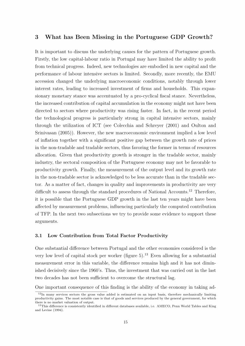
3.1 Low Contribution from Total Factor Productivity

One substantial difference between Portugal and the other economies considered is the

very low level of capital stock per worker (figure 5).13 Even allowing for a substantial

measurement error in this variable, the difference remains high and it has not dimin-

ished decisively since the 1960’s. Thus, the investment that was carried out in the last

two decades has not been sufficient to overcome the structural lag.

One important consequence of this finding is the ability of the economy in taking ad-12In many services sectors the gross value added is estimated on an input basis, therefore mechanically limiting

productivity gains. The most notable case is that of goods and services produced by the general government, for whichthere is no market valuation of output.

13This difference is consistently identified in different databases available, i.e. AMECO, Penn World Tables and Kingand Levine (1994).

15

Figure 5: Capital-Labour ratio� �

�

��

��

��

��

��

��

��

��

��

��

��

��

��

Portugal

Ireland

Greece

Spain

�� !�� "

(a) Percentage of OECD-21 average

�

��

��

��

��

��

��

�� !��"�#��$� ��%&'�%&��'��"�#%(

(b) OECD-21 average =100 (1995-2004)

vantage of the new production techniques that became internationally available. The

shape (figure 6) and the dynamics (figure 7) of the stochastic production frontiers re-

veal that technology favors higher capital-labour ratios, namely in recent decades, and

technological progress is relatively stronger for higher capital per worker intensities

notably in the sixties and nineties. In the recent periods the surface of the stochastic

production function seems to have became more convex, meaning that the technological

progress and potential TFP gains are centered in sectors with higher capital content.

Such finding is consistent with the idea that technology and productivity are essen-

tially associated with manufacturing and, more recently in ICT industries. Conversely,

services and construction, with lower capital per worker, are not so benefited from

technology. This would configure a poverty trap as low capital economies would be at

a disadvantage in terms of economic growth and such outcome would limit their ability

to invest. Nevertheless, the Portuguese case might not only be a story of investment

shortage but probably also a story of low investment quality that is linked with the

sectoral composition of economic activity.

The computed capital and labour elasticities, which are used to decompose factor’s

contribution to growth, offer a complementary perspective (see table 3). Portugal

shows high elasticities for capital, notably in the last decade, and labour elasticities

have decreased consistently, becoming lower than in other countries. Finally, the sum

of computed elasticities is relatively close to one in all countries and in all periods,

meaning that technology is near the constant returns to scale paradigm.

The sectoral composition of Portuguese output reveals that the quick decrease in agri-

culture’s relative weight was basically compensated by an increase in manufactures.

This brought and increase in capital intensity and TFP contribution. During the pe-

riod ranging from the mid-seventies to the mid-nineties the weight of manufactures

16

Figure 6: 3D stochastic production frontiers - Arrow points to Portuguese economy

34

56

78

7

8

9

10

11

0

1

2

3

4

5

6

7

8

ln(K)ln(L)

ln(Y)

(a) 1960

34

56

78

7

8

9

10

11

2

3

4

5

6

7

8

ln(K)ln(L)

ln(Y)

(b) 1965

34

56

78

7

8

9

10

11

2

3

4

5

6

7

8

ln(K)ln(L)

ln(Y)

(c) 1970

34

56

78

8

9

10

11

2

3

4

5

6

7

8

ln(K)ln(L)

ln(Y)

(d) 1975

45

67

8

8

9

10

11

2

3

4

5

6

7

8

ln(K)ln(L)

ln(Y)

(e) 1980

45

67

8

8

9

10

11

2

3

4

5

6

7

8

ln(K)ln(L)

ln(Y)

(f) 1985

45

67

89

8

9

10

11

2

3

4

5

6

7

8

9

ln(K)ln(L)

ln(Y)

(g) 1990

45

67

89

8

9

10

11

−4

−2

0

2

4

6

8

ln(K)ln(L)

ln(Y)

(h) 1995

17

Figure 7: Dynamic stochastic production frontiers (L level set for Portugal)

1960-70

��

��

��

��

��

��

� ��

��

��

��

K/L

��

��

��

��

��

��

��

��

��

�!�"�#$��

�%�

�%�

(a) 1960-70

1965-75

��

��

��

��

��

��

��

��

� ��

��

��

��

��

T=1

T=10

��

��

��

��

�� !�"#$%%

��

(b) 1965-75

��

��

��

��

��

��

��

��

��

� ��

�

��

��

��

��

T=1

T=10

��

��

Reference value for L = 3900

��

��

��

(c) 1970-80

��

��

��

��

��

��

��

��

��

� ��

�

� �

��

��

��

T=1

T=10

��

��


��

��

��

(d) 1975-85

��

��

��

��

��

��

��

��

��

��

��

� ��

��

��

��

��

��

��

��

��

��

��

��

��

T=1

T=10

��

��


��

��

��

(e) 1980-90

��

��

��

��

��

��

��

��

��

��

� ��

��

��

��

��

��

T=1

T=10

��


��

��

��

(f) 1985-95

��

��

��

��

��

��

��

��

��

��

��

� ��

��

��

��

��

��

��

��

��

��

��

��

��

��

T=1

T=10

��


��

��

��

(g) 1990-00

��

��

��

��

��

��

��

� ��

��

��

��

��

��

��

��

��

��

��

��

��

��

T=1

T=10

��

��


��

��

(h) 1995-05

18

��

��

��

��

��

��

��

��

��

� !"#�$%&'()*#+#" ,*-.-*-#,-/0&1*)2 "�3( -/�41##.# /+51#" /+6"&2 1-*7',8

9:;;<; =:;>?@A

BC?D@EF:GHI?>

remained broadly stable and the slower decline in agriculture was compensated by a

rise of services and construction. This somewhat limited the contribution of TFP to

economic growth.14 Finally, during the nineties manufactures joined to the downward

trend of agriculture and, consequently, the weight of services and construction has risen

faster. In fact the join weight of agriculture and manufacturing that represented almost

half of gross value added fifty years ago, was reduced to around 20 per cent in 2005

(figure 8).

The discussion on the quality of the investment that was made in Portugal is not linked

with factor intensity and its relation with technological progress but with the contri-

bution of efficiency to TFP. The results reveal that, although Portugal presents a good

level of efficiency in the utilization of resources comparatively to the other countries

considered (see figure 9 and Appendix C), the contribution of efficiency developments

was negative in the period 1965-75 and 1995-2005. Although there were significant

investments in labour intensive manufacturing sectors, like textiles and clothing, fol-

lowing the EFTA accession, in the period 1965-75 a substantial part of the investment

was directed to large capital intensive industries. Unfortunately, the increasing of ca-

pacity in these sectors almost coincided with negative developments in world markets.

A similar result seems to be present in the 1995-2005 period. This time it is not a story

14It is acknowledged that the non-tradable nature of many services sectors lowers competition, contributing to lowerproductivity gains. This is particularly relevant in the case of public services.

19

Figure 8: Sector shares in GVA

�

��

��

��

��

��

��

��

��

� ��

!��"��

#$%&'(&)*&+,)&-.*/��

($0)1&'2$)%030&+&#4(-/5,-/1$5&2$)%03-6

of investment in manufacturing capital intensive sectors, but probably investment in

real assets with low return such as housing. The considerations on the quality of pro-

duction factors are extendable to labour, as Portugal presents severe shortcomings in

terms of average number of schooling years. Moreover, the institutional aspects of the

Portuguese labour market may have been playing a role. There seems to be a lack

of labour mobility, which is confined almost entirely to fixed-term contracts, making

difficult efficient matches between workers’ skills and labour services needed by firms

(see Blanchard and Portugal (2001)).

Nevertheless, considerations on the quality of production factors should be addressed

specifically by including adjustment parameters in the production function like in Koop,

Osiewalski and Steel (2000). In this case a bilinear production function is used to

account for the effect of different characteristics of inputs. This is a research path to

follow in future work.

3.2 GDP Measurement Problems

The measurement of economic activity in the non-tradables sector, where the produc-

tion is often of an immaterial nature, faces difficulties that may limit its accuracy.

Although the weight of this sector is clearly dominant and it has been continually

increasing in the developed economies, the underlying statistical infrastructure of na-

tional accounts has not improved proportionally. In fact, there is lack of reliable and

internationally comparable statistical indicators for some important services activities,

notably, services provided by general government (figure 10).

These measurement problems associated to the non-tradables sector tend to affect all

countries, but with different magnitudes. Therefore, when comparing growth account-

20

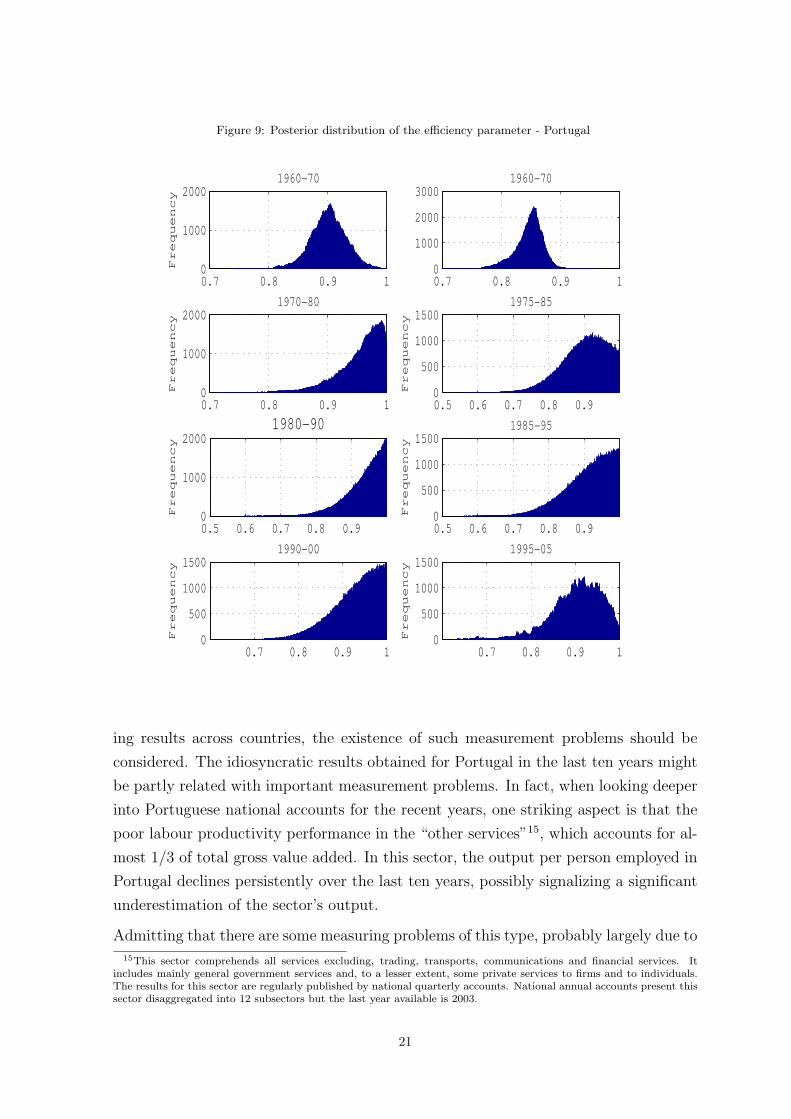
Figure 9: Posterior distribution of the efficiency parameter - Portugal

0.7 0.8 0.9 10

1000

2000

Fre

qu

en

cy

1960−70

0.7 0.8 0.9 10

1000

2000

30001960−70

0.7 0.8 0.9 10

1000

2000

Fre

qu

en

cy

1970−80

0.5 0.6 0.7 0.8 0.90

500

1000

1500

Fre

qu

en

cy

1975−85

0.5 0.6 0.7 0.8 0.90

1000

2000

Fre

qu

en

cy

1980−90

0.5 0.6 0.7 0.8 0.90

500

1000

1500

Fre

qu

en

cy

1985−95

0.7 0.8 0.9 10

500

1000

1500

Fre

qu

en

cy

1990−00

0.7 0.8 0.9 10

500

1000

1500

Fre

qu

en

cy

1995−05

ing results across countries, the existence of such measurement problems should be

considered. The idiosyncratic results obtained for Portugal in the last ten years might

be partly related with important measurement problems. In fact, when looking deeper

into Portuguese national accounts for the recent years, one striking aspect is that the

poor labour productivity performance in the “other services”15, which accounts for al-

most 1/3 of total gross value added. In this sector, the output per person employed in

Portugal declines persistently over the last ten years, possibly signalizing a significant

underestimation of the sector’s output.

Admitting that there are some measuring problems of this type, probably largely due to

15This sector comprehends all services excluding, trading, transports, communications and financial services. Itincludes mainly general government services and, to a lesser extent, some private services to firms and to individuals.The results for this sector are regularly published by national quarterly accounts. National annual accounts present thissector disaggregated into 12 subsectors but the last year available is 2003.

21

Figure 10: Weight of general government consumption on GDP

�

�

��

��

��

��

��

��

��

��

��

Portugal

IrelandSpain

Greece

�� !�"#�$%&'$%��&�� $(

the way general government real output is measured, we performed two simulations for

the period 1995-2005 under the assumption that employment and capital levels are not

significantly affected by this problem. In the first simulation, we artificially increased

labour productivity annual rate of change of “other services” to match the average

annual rate of change in the rest of the economy. In the second one, we set labour

productivity annual rate of change of “other services” equal to zero. The average

GDP annual growth rates where revised upwards by 0.9 and 0.3 percentage points,

respectively. 16 As expected, the upward revision in GDP growth is reflected in a less

negative (in the second simulation) or even in a slightly positive contribution of total

factor productivity (in the first simulation).17 However, it is worth noting that the

contribution of efficiency remains negative and almost unchanged in the two exercises

while the contribution of technical progress, which was strongly negative, turns positive

in the first simulation.

Although these exercises illustrate that measurement problems may have their share

in explaining the poor performance of the Portuguese economy expressed in national

accounts, the results obtained with simulations show that the increases in TFP con-

tribution are not very strong, meaning that the other aspects must remain part of the

explanation.

16The assumption of maintaining unchanged the employment and stock of capital levels is not unreasonable. Thestock of capital evolution reflects mainly the dynamic of GFCF which is recorded as the sum of expenditures of residentsin equipment, transportation and construction goods. So if there is a problem of missing output in “other services” thereare no strong reasons to believe that it would also significantly affect the measure of those two variables (employmentand GFCF). Moreover, if an upward revision of the “other services” output takes place, in the expenditure side, it wouldbe reflected mainly in more private and general government consumptions.

17As the estimation is made jointly for all the countries considered, the changes in Portugal affect not only its resultsbut also the results of the other countries. However, no noticeable changes were in fact detected in the results for theother countries.

22

4 Final Remarks

This paper develops a growth accounting exercise for the Portuguese economy in the

last four decades, setting Spain, Greece and Ireland as a benchmark. The technical

approach adopted here is superior to the typical growth accounting methodology. In

this paper a dynamic translog world stochastic production frontier is computed, pro-

viding a more accurate accounting of inputs and TFP contribution, allowing for the

decomposition of the latter into technical progress and efficiency.

We conclude that Portugal derived much of its economic growth from capital accumu-

lation, whereas labour input showed systematic low contributions. The contribution

of TFP was lower than in the other benchmark countries, particularly in the last

decade. Some explanations for the poor performance of TFP are proposed, basing on

its decomposition. Firstly, the capital-labour ratio in Portugal is low in international

terms, which does not allow to fully capture the benefits of technological progress. As

a matter of fact, the expansion in the world production function is larger for higher

capital intensities and its shape favours larger capital ratios. Secondly, the quality of

the investment and other institutional factors seem to lead to a low contribution of

efficiency improvements to GDP growth, thereby contributing to a poor overall TFP

performance. Finally, the hypothesis of measurement problems in the Portuguese GDP,

if confirmed, is reflected in the apparent poor performance of TFP. However, given its

possible magnitude, it should not change the general picture.

There is clearly scope for further research in this area, namely adjusting capital and

labour stocks by their quality to assess how changes in such characteristics affect GDP

growth accounting.

23

References

Aigner, D., Lovell, C. and Schmidt, P. (1977), ‘Formulation and estimation of stochastic

frontier production function models’, Journal of Econometrics (6), 21–37.

Almeida, V. and Felix, R. (2006), ‘Computing potential output and the output gap for

the portuguese economy’, Banco de Portugal Economic Bulletin .

Barro, R. (1991), ‘Economic growth in a cross section of countries’, Quarterly Journal

of Economics 106, 407–433.

Basu, W. and Weil, D. (1998), ‘Appropriate technology and growth’, Quarterly Journal

of Economics 113, 1025–1054.

Baumol, W. (1986), ‘Productivity growth, convergence, and welfare: What the long-

run data show’, American Economic Review 76(5), 1072–85.

Berndt, E. and Triplett, J. (1990), Fifty Years of Economic Measurement, University

of Chicago Press.

Blanchard, O. and Portugal, P. (2001), ‘What hides behind an unemployment rate:

Comparing portuguese and u.s. labor markets’, American Economic Review 1(91).

Casella, G. and George, E. (1992), ‘Explaining the gibbs sampler’, The American

Statistician (46), 167–174.

Colecchia, A. and Schreyer, P. (2001), Ict investment and economic growth in the

1990’s: is the united states a unique case? a comparative study of nine oecd

countries, Technical Report OECD DSTI/DOC 2001/7, October.

Cornwell, C., Schmidt, P. and Sickles, R. (1990), ‘Production frontiers with cross-

sectional and time-series variation in efficiency levels’, Journal of Econometrics

46(1), 185–200.

Freitas, M. L. (2000), ‘Quantity versus quality: The growth accounting in ireland’,

Banco de Portugal Economic Bulletin .

Geweke, J. (1992), Evaluating the accuracy of sampling based approaches to the cal-

culation of posterior moments, in J. M. B. et al., ed., ‘Bayesian Statistics 4: Pro-

ceedings of the Fourth Valencia International Meeting’, Oxford Clarendon Press.

Greene, W. (2000), ‘Simulated likelihood estimation of the normal-gamma stochastic

frontier function’, Quarterly Journal of Economics 113, 1025–1054.

Griffin, J. and Steel, M. (2004), ‘Semiparametric bayesian inference for stochastic fron-

tier models’, Journal of Econometrics (123), 121–152.

24

King, R. and Levine, R. (1994), ‘Capital fundamentalism, economic development, and

economic growth’, Carnegie-Rochester Conference Series on Public Policy 40, 259–

292.

Koop, G., Osiewalski, J. and Steel, M. (1999), ‘The components of output growth:

A stochastic frontier analysis’, Oxford Bulletin of Economics and Statistics

61(4), 455–487.

Koop, G., Osiewalski, J. and Steel, M. (2000), ‘Modelling the sources of output growth

in a panel of countries’, Journal of Business & Economic Statistics 18(3), 284–299.

Kumbhakar, S. C. and Lovell, C. (2004), Stochastic Frontier Analysis, Cambridge Uni-

versity Press.

Lopes, S. (1999), A Economia Portuguesa desde 1960, Gradiva.

Lucas, R. (1988), ‘On the mechanics of economic development’, Journal of Monetary

Economics 22, 3–42.

Meeusen, W. and der Broeck, V. (1977), ‘Efficiency estimation from cobb-douglas pro-

duction functions with composed error’, International Economic Review (18), 435–

452.

Oulton, N. and Srinivasan, S. (2005), Productivity growth and the role of ict in the

united kigdom: An industry view 1970-2000, Technical Report 681.

Perelman, S. and Pestieau, P. (1994), ‘A comparative performance study of postal

services: A productive efficiency approach’, Annales de Economie et de Statistique

33, 187–202.

Romer, P. (1986), ‘Increasing returns and long-run growth’, Journal of Political Econ-

omy 94(5), 1002–1037.

Romer, P. (1990), ‘Endogenous technological change’, Journal of Political Economy

98(5), 71–102.

Sala-Martin, X. (1997), ‘I just ran 2 million regressions’, American Economic Review

87(2), 178–183.

Solow, R. (1956), ‘A contribution to the theory of economic growth’, Quarterly Journal

of Economics 70, 65–34.

Solow, R. (1957), ‘Technical change and the aggregate production function’, Review of

Economics and Statistics 39, 312–320.

Sousa, A. (1995), ‘Os anos 60 da nossa economia’, Analise Social .

25

Temple, J. (2006), ‘Aggregate production functions and growth economics’, Interna-

tional Review of Applied Economics 20(3), 301–317.

Tsionas, E. (2000), ‘Full likelihood inference in normal-gamma stochastic frontier mod-

els’, Journal of Productivity Analysis 13, 183–205.

26

Appendices

A The Marginal Posterior Distributions

The model to estimate is of the form:

Y = X∗β + v − u

where v is the error term and u is the efficiency parameter, which is function of para-

meter λ (u = f (λ)).

The full posterior distribution of the model is:

P(β, u, λ, σ2|Y )

∝ P(Y |β, u, λ, σ2

)P

(β, u, λ, σ2

)

where the first term is the likelihood function. Therefore:

P(β, u, λ, σ2

)∝ P (β) P

(σ2

) T∏t=1

N∏i=1

P(ui|λ−1

)P

(λ−1

)

The prior distribution for the parameter λ is a gamma with parameters 1 and τ ∗:

P (λ) = fG (λ|1,− ln (τ ∗))

∝ − ln (τ ∗) eln(τ∗)λ−1

The prior distribution for the parameter σ−2 is given by:

P(σ−2

)= σ−2(n0

2−1) exp

(− a0

2σ2

)

∝ σ−2(n02−1)ao

2e−

a02σ2

where a0 = 10−6 is the usual non-informative prior.

The prior for u|λ−1 is an exponential function:

P(u|λ−1

)∝

T∏t=1

N∏i=1

1

λe−

1λ

uit

The likelihood function is defined as a multivariate normal distribution:

P(Y |β, u, λ, σ2

)∝ σ2(−NT

2 )e{− 12σ2 (Y−X∗β+u)′(Y−X∗β+u)}

Therefore, the conditional posterior for the parameter β is:

exp

{− 1

2σ2(Y −X∗β + u)′ (Y −X∗β + u)

}

27

which after decomposing and eliminating constants gives:

∝ N12(β|β − (X∗′X∗) X∗ (Y + u) , σ−2 (X∗′X∗)−1

)

The conditional posterior for σ−2 is:(σ−2

(n0

2− 1

) a0

2e(

−a02σ2 )

)σ−2(NT

2 )e−1

2σ2 (Y−X∗β+u)′(Y−X∗β+u)

σ−2(n0+NT2

−1)e−�

a0+(Y−X∗β+u)′(Y−X∗β+u)2

�σ−2

which gives raise to the gamma distribution:

∝ G

(n0 + NT

2,1

2

(a0 + (Y −X∗β + u)′ (Y −X∗β + u)

))

The λ parameter has the following conditional posterior:

− ln (τ ∗) eln(τ∗)λT∏

t=1

N∏i=1

λe−λuit .λNT e−λ

− ln(τ∗)+

NPi

TPt

uit

!

which leads to a gamma distribution:

∝ G

(λ,NT + 1,− ln (τ ∗) +

N∑i

T∑t

uit

)

Finally, the conditional posterior distribution for u is:

T∏t=1

N∏i=1

λe−λuit .e−1

2σ2 (u′u+2Y ′u−2X∗βu)

meaning a multivariate normal distribution:

∝ NTN(u|X∗β − Y − λσ2i, σ2

)

28

B Growth Accounting in Spain, Greece and Ireland

��

��

��

�� ! " !## !" !$"�� %�� ! & !## !"' !"'�� %�� ! ' !$ #!#( #! (�� %�� #!#) !$* !(+ #!""�� %��#!+# !#$ !() #!+(�� %��#!+( ! ' !(' #!&"�� %��#!" !# !($ #!+$�� %�� %�� ! " ! * !$* !$$,-./01234/5676.236855.279:-;67./;<42;.63/;27=/5

��

��

��

�� %�� ! " !#) !"& !+#�� %�� %�� ! + !#+ !$# !$"�� %�� ! ) !#* !+" !+"�� %�� %��#!#* !#$ !&& #!$*�� %��#!+* ! ) !(+ #!& �� %��#!($ ! ) !(( #!)&�� %��#!+# ! ( !(# #!&(�� ! " ! & !" !$',-./01234/5676.236855.279:-;67./;<42;.63/;27=/5

Spain

>��?�@��

A@��B�?C>D��

�E ��?C>D��

F� �� ?��B��

Greece

>��?�@��

A@��B�?C>D��

�E ��?C>D��

F� �� ?��B��

29

��

��

��

��

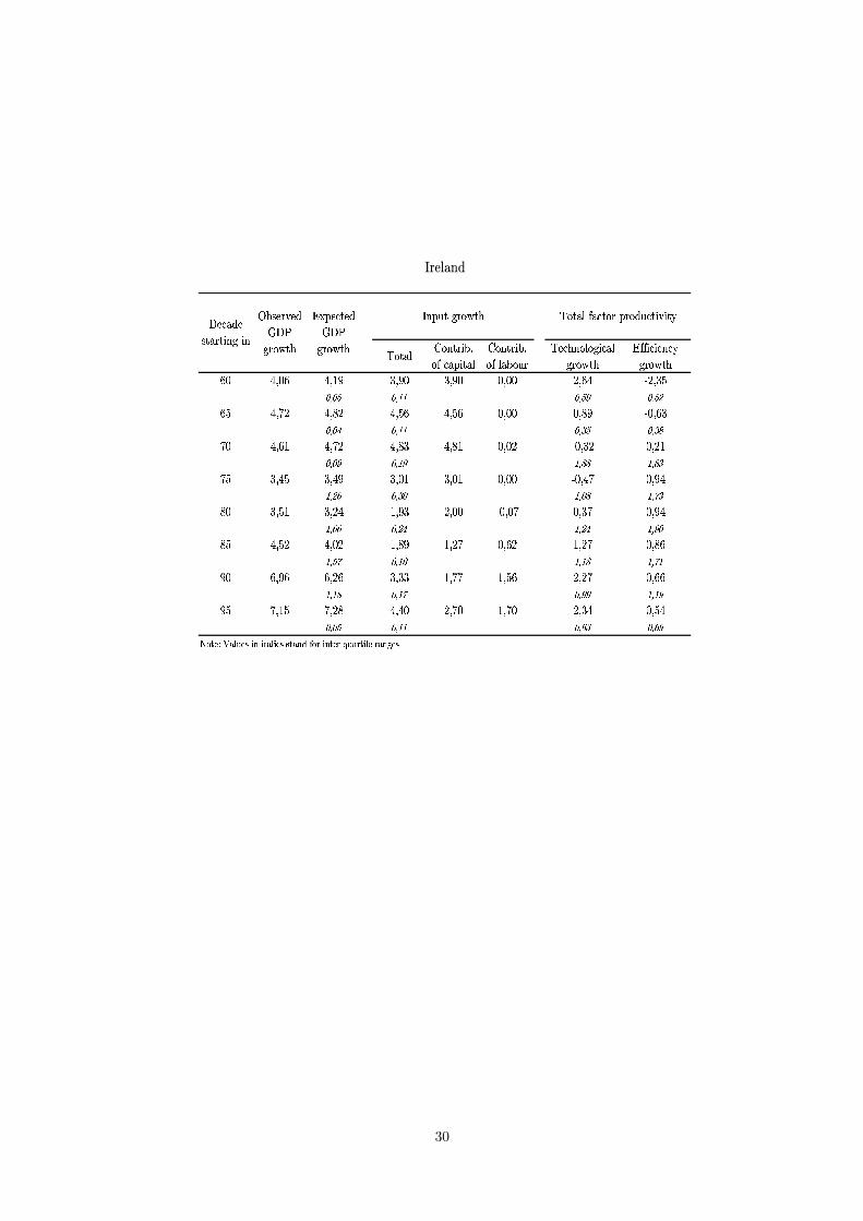
�� ! � "" � !# � !$�� %� ��&� �� &� �� ' � "" � (! � ()%� �� %� ��&� ��&� �� # � "# " )) " )(%� �� % ��" $* � (� " �) " +(&� �� % ��% ��" ** � $' " $' " #�&� �� &� ��% �� % ��&�" !+ � "� " ") " +"�� %% �� % ��" ") � "+ � ## " "#�� %�� %��& �� %� ��%� �� ! � "" � *( � *#,-./01234/5676.236855.279:-;67./;<42;.63/;27=/5

Ireland

>��?�@��

A@��B�?C>D

��

�E ��?C>D

��

F� �� ?��B��

30

C Posterior Distribution of the Efficiency Parameter

Figure 11: Posterior distribution of the efficiency parameter - Spain

0.7 0.75 0.8 0.85 0.90

1000

2000

3000

Fre

qu

en

cy

1960−70

0.65 0.7 0.75 0.8 0.850

1000

2000

3000

Fre

qu

en

cy

1965−75

0.7 0.8 0.9 10

1000

2000

3000

Fre

qu

en

cy

1970−80

0.5 0.6 0.7 0.8 0.90

500

1000

1500

Fre

qu

en

cy

1975−85

0.5 0.6 0.7 0.8 0.90

500

1000

Fre

qu

en

cy

1980−90

0.5 0.6 0.7 0.8 0.90

500

1000

Fre

qu

en

cy

1985−95

0.5 0.6 0.7 0.8 0.90

500

1000

Fre

qu

en

cy

1990−00

0.65 0.7 0.750

1000

2000

3000

Fre

qu

en

cy

1995−05

31

Figure 12: Posterior distribution of the efficiency parameter - Greece

0.9 0.95 10

2000

4000

Fre

qu

en

cy

1960−70

0.75 0.8 0.85 0.9 0.950

2000

4000

Fre

qu

en

cy

1965−75

0.7 0.8 0.9 10

2000

4000

Fre

qu

en

cy

1970−80

0.5 0.6 0.7 0.8 0.90

500

1000

1500

Fre

qu

en

cy

1975−85

0.5 0.6 0.7 0.8 0.90

500

1000

Fre

qu

en

cy

1980−90

0.4 0.6 0.8 10

500

1000

1500

Fre

qu

en

cy

1985−95

0.4 0.6 0.8 10

500

1000

1500

Fre

qu

en

cy

1990−00

0.55 0.6 0.650

1000

2000

3000

Fre

qu

en

cy

1995−05

32

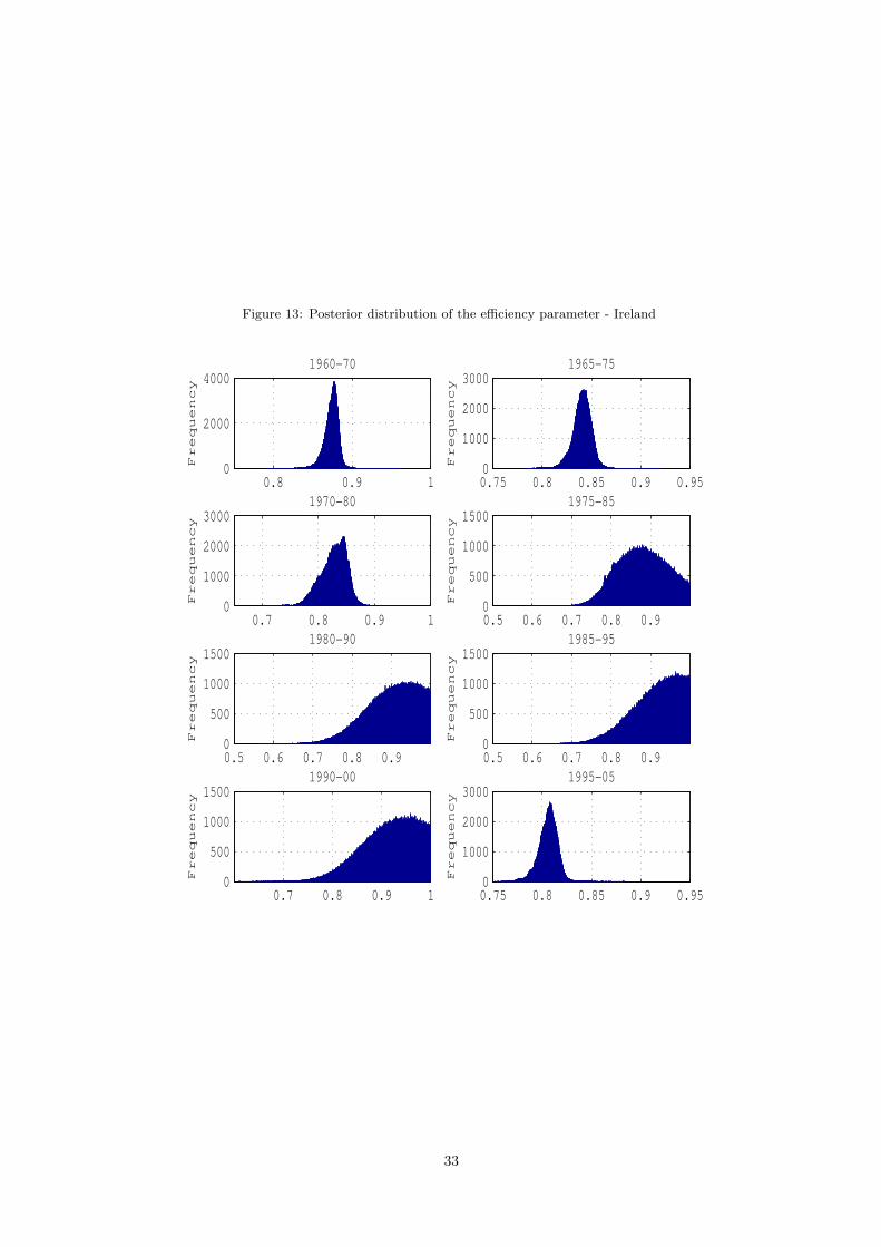
Figure 13: Posterior distribution of the efficiency parameter - Ireland

0.8 0.9 10

2000

4000

Fre

qu

en

cy

1960−70

0.75 0.8 0.85 0.9 0.950

1000

2000

3000

Fre

qu

en

cy

1965−75

0.7 0.8 0.9 10

1000

2000

3000

Fre

qu

en

cy

1970−80

0.5 0.6 0.7 0.8 0.90

500

1000

1500

Fre

qu

en

cy

1975−85

0.5 0.6 0.7 0.8 0.90

500

1000

1500

Fre

qu

en

cy

1980−90

0.5 0.6 0.7 0.8 0.90

500

1000

1500

Fre

qu

en

cy

1985−95

0.7 0.8 0.9 10

500

1000

1500

Fre

qu

en

cy

1990−00

0.75 0.8 0.85 0.9 0.950

1000

2000

3000

Fre

qu

en

cy

1995−05

33

WORKING PAPERS

2000

1/00 UNEMPLOYMENT DURATION: COMPETING AND DEFECTIVE RISKS

— John T. Addison, Pedro Portugal

2/00 THE ESTIMATION OF RISK PREMIUM IMPLICIT IN OIL PRICES

— Jorge Barros Luís

3/00 EVALUATING CORE INFLATION INDICATORS

— Carlos Robalo Marques, Pedro Duarte Neves, Luís Morais Sarmento

4/00 LABOR MARKETS AND KALEIDOSCOPIC COMPARATIVE ADVANTAGE

— Daniel A. Traça

5/00 WHY SHOULD CENTRAL BANKS AVOID THE USE OF THE UNDERLYING INFLATION INDICATOR?

— Carlos Robalo Marques, Pedro Duarte Neves, Afonso Gonçalves da Silva

6/00 USING THE ASYMMETRIC TRIMMED MEAN AS A CORE INFLATION INDICATOR

— Carlos Robalo Marques, João Machado Mota

2001

1/01 THE SURVIVAL OF NEW DOMESTIC AND FOREIGN OWNED FIRMS

— José Mata, Pedro Portugal

2/01 GAPS AND TRIANGLES

— Bernardino Adão, Isabel Correia, Pedro Teles

3/01 A NEW REPRESENTATION FOR THE FOREIGN CURRENCY RISK PREMIUM

— Bernardino Adão, Fátima Silva

4/01 ENTRY MISTAKES WITH STRATEGIC PRICING

— Bernardino Adão

5/01 FINANCING IN THE EUROSYSTEM: FIXED VERSUS VARIABLE RATE TENDERS

— Margarida Catalão-Lopes

6/01 AGGREGATION, PERSISTENCE AND VOLATILITY IN A MACROMODEL

— Karim Abadir, Gabriel Talmain

7/01 SOME FACTS ABOUT THE CYCLICAL CONVERGENCE IN THE EURO ZONE

— Frederico Belo

8/01 TENURE, BUSINESS CYCLE AND THE WAGE-SETTING PROCESS

— Leandro Arozamena, Mário Centeno

9/01 USING THE FIRST PRINCIPAL COMPONENT AS A CORE INFLATION INDICATOR

— José Ferreira Machado, Carlos Robalo Marques, Pedro Duarte Neves, Afonso Gonçalves da Silva

10/01 IDENTIFICATION WITH AVERAGED DATA AND IMPLICATIONS FOR HEDONIC REGRESSION STUDIES

— José A.F. Machado, João M.C. Santos Silva

Banco de Portugal | Working Papers i

2002

1/02 QUANTILE REGRESSION ANALYSIS OF TRANSITION DATA

— José A.F. Machado, Pedro Portugal

2/02 SHOULD WE DISTINGUISH BETWEEN STATIC AND DYNAMIC LONG RUN EQUILIBRIUM IN ERROR

CORRECTION MODELS?

— Susana Botas, Carlos Robalo Marques

3/02 MODELLING TAYLOR RULE UNCERTAINTY

— Fernando Martins, José A. F. Machado, Paulo Soares Esteves

4/02 PATTERNS OF ENTRY, POST-ENTRY GROWTH AND SURVIVAL: A COMPARISON BETWEEN DOMESTIC AND

FOREIGN OWNED FIRMS

— José Mata, Pedro Portugal

5/02 BUSINESS CYCLES: CYCLICAL COMOVEMENT WITHIN THE EUROPEAN UNION IN THE PERIOD 1960-1999. A

FREQUENCY DOMAIN APPROACH

— João Valle e Azevedo

6/02 AN “ART”, NOT A “SCIENCE”? CENTRAL BANK MANAGEMENT IN PORTUGAL UNDER THE GOLD STANDARD,

1854 -1891

— Jaime Reis

7/02 MERGE OR CONCENTRATE? SOME INSIGHTS FOR ANTITRUST POLICY

— Margarida Catalão-Lopes

8/02 DISENTANGLING THE MINIMUM WAGE PUZZLE: ANALYSIS OF WORKER ACCESSIONS AND SEPARATIONS

FROM A LONGITUDINAL MATCHED EMPLOYER-EMPLOYEE DATA SET

— Pedro Portugal, Ana Rute Cardoso

9/02 THE MATCH QUALITY GAINS FROM UNEMPLOYMENT INSURANCE

— Mário Centeno

10/02 HEDONIC PRICES INDEXES FOR NEW PASSENGER CARS IN PORTUGAL (1997-2001)

— Hugo J. Reis, J.M.C. Santos Silva

11/02 THE ANALYSIS OF SEASONAL RETURN ANOMALIES IN THE PORTUGUESE STOCK MARKET

— Miguel Balbina, Nuno C. Martins

12/02 DOES MONEY GRANGER CAUSE INFLATION IN THE EURO AREA?

— Carlos Robalo Marques, Joaquim Pina

13/02 INSTITUTIONS AND ECONOMIC DEVELOPMENT: HOW STRONG IS THE RELATION?

— Tiago V.de V. Cavalcanti, Álvaro A. Novo

2003

1/03 FOUNDING CONDITIONS AND THE SURVIVAL OF NEW FIRMS

— P.A. Geroski, José Mata, Pedro Portugal

2/03 THE TIMING AND PROBABILITY OF FDI: AN APPLICATION TO THE UNITED STATES MULTINATIONAL

ENTERPRISES

— José Brandão de Brito, Felipa de Mello Sampayo

3/03 OPTIMAL FISCAL AND MONETARY POLICY: EQUIVALENCE RESULTS

— Isabel Correia, Juan Pablo Nicolini, Pedro Teles

Banco de Portugal | Working Papers ii

4/03 FORECASTING EURO AREA AGGREGATES WITH BAYESIAN VAR AND VECM MODELS

— Ricardo Mourinho Félix, Luís C. Nunes

5/03 CONTAGIOUS CURRENCY CRISES: A SPATIAL PROBIT APPROACH

— Álvaro Novo

6/03 THE DISTRIBUTION OF LIQUIDITY IN A MONETARY UNION WITH DIFFERENT PORTFOLIO RIGIDITIES

— Nuno Alves

7/03 COINCIDENT AND LEADING INDICATORS FOR THE EURO AREA: A FREQUENCY BAND APPROACH

— António Rua, Luís C. Nunes

8/03 WHY DO FIRMS USE FIXED-TERM CONTRACTS?

— José Varejão, Pedro Portugal

9/03 NONLINEARITIES OVER THE BUSINESS CYCLE: AN APPLICATION OF THE SMOOTH TRANSITION

AUTOREGRESSIVE MODEL TO CHARACTERIZE GDP DYNAMICS FOR THE EURO-AREA AND PORTUGAL

— Francisco Craveiro Dias

10/03 WAGES AND THE RISK OF DISPLACEMENT

— Anabela Carneiro, Pedro Portugal

11/03 SIX WAYS TO LEAVE UNEMPLOYMENT

— Pedro Portugal, John T. Addison

12/03 EMPLOYMENT DYNAMICS AND THE STRUCTURE OF LABOR ADJUSTMENT COSTS


13/03 THE MONETARY TRANSMISSION MECHANISM: IS IT RELEVANT FOR POLICY?


14/03 THE IMPACT OF INTEREST-RATE SUBSIDIES ON LONG-TERM HOUSEHOLD DEBT: EVIDENCE FROM A

LARGE PROGRAM

— Nuno C. Martins, Ernesto Villanueva

15/03 THE CAREERS OF TOP MANAGERS AND FIRM OPENNESS: INTERNAL VERSUS EXTERNAL LABOUR

MARKETS

— Francisco Lima, Mário Centeno

16/03 TRACKING GROWTH AND THE BUSINESS CYCLE: A STOCHASTIC COMMON CYCLE MODEL FOR THE EURO

AREA

— João Valle e Azevedo, Siem Jan Koopman, António Rua

17/03 CORRUPTION, CREDIT MARKET IMPERFECTIONS, AND ECONOMIC DEVELOPMENT

— António R. Antunes, Tiago V. Cavalcanti

18/03 BARGAINED WAGES, WAGE DRIFT AND THE DESIGN OF THE WAGE SETTING SYSTEM

— Ana Rute Cardoso, Pedro Portugal

19/03 UNCERTAINTY AND RISK ANALYSIS OF MACROECONOMIC FORECASTS: FAN CHARTS REVISITED

— Álvaro Novo, Maximiano Pinheiro

2004

1/04 HOW DOES THE UNEMPLOYMENT INSURANCE SYSTEM SHAPE THE TIME PROFILE OF JOBLESS

DURATION?

— John T. Addison, Pedro Portugal

Banco de Portugal | Working Papers iii

2/04 REAL EXCHANGE RATE AND HUMAN CAPITAL IN THE EMPIRICS OF ECONOMIC GROWTH

— Delfim Gomes Neto

3/04 ON THE USE OF THE FIRST PRINCIPAL COMPONENT AS A CORE INFLATION INDICATOR

— José Ramos Maria

4/04 OIL PRICES ASSUMPTIONS IN MACROECONOMIC FORECASTS: SHOULD WE FOLLOW FUTURES MARKET

EXPECTATIONS?

— Carlos Coimbra, Paulo Soares Esteves

5/04 STYLISED FEATURES OF PRICE SETTING BEHAVIOUR IN PORTUGAL: 1992-2001

— Mónica Dias, Daniel Dias, Pedro D. Neves

6/04 A FLEXIBLE VIEW ON PRICES

— Nuno Alves

7/04 ON THE FISHER-KONIECZNY INDEX OF PRICE CHANGES SYNCHRONIZATION

— D.A. Dias, C. Robalo Marques, P.D. Neves, J.M.C. Santos Silva

8/04 INFLATION PERSISTENCE: FACTS OR ARTEFACTS?

— Carlos Robalo Marques

9/04 WORKERS’ FLOWS AND REAL WAGE CYCLICALITY


10/04 MATCHING WORKERS TO JOBS IN THE FAST LANE: THE OPERATION OF FIXED-TERM CONTRACTS


11/04 THE LOCATIONAL DETERMINANTS OF THE U.S. MULTINATIONALS ACTIVITIES

— José Brandão de Brito, Felipa Mello Sampayo

12/04 KEY ELASTICITIES IN JOB SEARCH THEORY: INTERNATIONAL EVIDENCE

— John T. Addison, Mário Centeno, Pedro Portugal

13/04 RESERVATION WAGES, SEARCH DURATION AND ACCEPTED WAGES IN EUROPE

— John T. Addison, Mário Centeno, Pedro Portugal

14/04 THE MONETARY TRANSMISSION N THE US AND THE EURO AREA: COMMON FEATURES AND COMMON

FRICTIONS

— Nuno Alves

15/04 NOMINAL WAGE INERTIA IN GENERAL EQUILIBRIUM MODELS

— Nuno Alves

16/04 MONETARY POLICY IN A CURRENCY UNION WITH NATIONAL PRICE ASYMMETRIES

— Sandra Gomes

17/04 NEOCLASSICAL INVESTMENT WITH MORAL HAZARD

— João Ejarque

18/04 MONETARY POLICY WITH STATE CONTINGENT INTEREST RATES


19/04 MONETARY POLICY WITH SINGLE INSTRUMENT FEEDBACK RULES


20/04 ACOUNTING FOR THE HIDDEN ECONOMY: BARRIERS TO LAGALITY AND LEGAL FAILURES

— António R. Antunes, Tiago V. Cavalcanti

Banco de Portugal | Working Papers iv

2005

1/05 SEAM: A SMALL-SCALE EURO AREA MODEL WITH FORWARD-LOOKING ELEMENTS

— José Brandão de Brito, Rita Duarte

2/05 FORECASTING INFLATION THROUGH A BOTTOM-UP APPROACH: THE PORTUGUESE CASE

— Cláudia Duarte, António Rua

3/05 USING MEAN REVERSION AS A MEASURE OF PERSISTENCE

— Daniel Dias, Carlos Robalo Marques

4/05 HOUSEHOLD WEALTH IN PORTUGAL: 1980-2004

— Fátima Cardoso, Vanda Geraldes da Cunha

5/05 ANALYSIS OF DELINQUENT FIRMS USING MULTI-STATE TRANSITIONS

— António Antunes

6/05 PRICE SETTING IN THE AREA: SOME STYLIZED FACTS FROM INDIVIDUAL CONSUMER PRICE DATA

— Emmanuel Dhyne, Luis J. Álvarez, Hervé Le Bihan, Giovanni Veronese, Daniel Dias, Johannes Hoffmann,

Nicole Jonker, Patrick Lünnemann, Fabio Rumler, Jouko Vilmunen

7/05 INTERMEDIATION COSTS, INVESTOR PROTECTION AND ECONOMIC DEVELOPMENT

— António Antunes, Tiago Cavalcanti, Anne Villamil

8/05 TIME OR STATE DEPENDENT PRICE SETTING RULES? EVIDENCE FROM PORTUGUESE MICRO DATA

— Daniel Dias, Carlos Robalo Marques, João Santos Silva

9/05 BUSINESS CYCLE AT A SECTORAL LEVEL: THE PORTUGUESE CASE

— Hugo Reis

10/05 THE PRICING BEHAVIOUR OF FIRMS IN THE EURO AREA: NEW SURVEY EVIDENCE

— S. Fabiani, M. Druant, I. Hernando, C. Kwapil, B. Landau, C. Loupias, F. Martins, T. Mathä, R. Sabbatini, H.

Stahl, A. Stokman

11/05 CONSUMPTION TAXES AND REDISTRIBUTION

— Isabel Correia

12/05 UNIQUE EQUILIBRIUM WITH SINGLE MONETARY INSTRUMENT RULES


13/05 A MACROECONOMIC STRUCTURAL MODEL FOR THE PORTUGUESE ECONOMY

— Ricardo Mourinho Félix

14/05 THE EFFECTS OF A GOVERNMENT EXPENDITURES SHOCK

— Bernardino Adão, José Brandão de Brito

15/05 MARKET INTEGRATION IN THE GOLDEN PERIPHERY – THE LISBON/LONDON EXCHANGE, 1854-1891

— Rui Pedro Esteves, Jaime Reis, Fabiano Ferramosca

2006

1/06 THE EFFECTS OF A TECHNOLOGY SHOCK IN THE EURO AREA

— Nuno Alves , José Brandão de Brito , Sandra Gomes, João Sousa

2/02 THE TRANSMISSION OF MONETARY AND TECHNOLOGY SHOCKS IN THE EURO AREA

— Nuno Alves, José Brandão de Brito, Sandra Gomes, João Sousa

Banco de Portugal | Working Papers v

3/06 MEASURING THE IMPORTANCE OF THE UNIFORM NONSYNCHRONIZATION HYPOTHESIS

— Daniel Dias, Carlos Robalo Marques, João Santos Silva

4/06 THE PRICE SETTING BEHAVIOUR OF PORTUGUESE FIRMS EVIDENCE FROM SURVEY DATA

— Fernando Martins

5/06 STICKY PRICES IN THE EURO AREA: A SUMMARY OF NEW MICRO EVIDENCE

— L. J. Álvarez, E. Dhyne, M. Hoeberichts, C. Kwapil, H. Le Bihan, P. Lünnemann, F. Martins, R. Sabbatini,

H. Stahl, P. Vermeulen and J. Vilmunen

6/06 NOMINAL DEBT AS A BURDEN ON MONETARY POLICY

— Javier Díaz-Giménez, Giorgia Giovannetti , Ramon Marimon, Pedro Teles

7/06 A DISAGGREGATED FRAMEWORK FOR THE ANALYSIS OF STRUCTURAL DEVELOPMENTS IN PUBLIC

FINANCES

— Jana Kremer, Cláudia Rodrigues Braz, Teunis Brosens, Geert Langenus, Sandro Momigliano, Mikko

Spolander

8/06 IDENTIFYING ASSET PRICE BOOMS AND BUSTS WITH QUANTILE REGRESSIONS

— José A. F. Machado, João Sousa

9/06 EXCESS BURDEN AND THE COST OF INEFFICIENCY IN PUBLIC SERVICES PROVISION

— António Afonso, Vítor Gaspar

10/06 MARKET POWER, DISMISSAL THREAT AND RENT SHARING: THE ROLE OF INSIDER AND OUTSIDER

FORCES IN WAGE BARGAINING


11/06 MEASURING EXPORT COMPETITIVENESS: REVISITING THE EFFECTIVE EXCHANGE RATE WEIGHTS FOR

THE EURO AREA COUNTRIES

— Paulo Soares Esteves, Carolina Reis

12/06 THE IMPACT OF UNEMPLOYMENT INSURANCE GENEROSITY

ON MATCH QUALITY DISTRIBUTION

— Mário Centeno, Alvaro A. Novo

13/06 U.S. UNEMPLOYMENT DURATION: HAS LONG BECOME LONGER OR SHORT BECOME SHORTER?

— José A.F. Machado, Pedro Portugal e Juliana Guimarães

14/06 EARNINGS LOSSES OF DISPLACED WORKERS: EVIDENCE FROM A MATCHED EMPLOYER-EMPLOYEE

DATA SET


15/06 COMPUTING GENERAL EQUILIBRIUM MODELS WITH OCCUPATIONAL CHOICE AND FINANCIAL FRICTIONS

— António Antunes, Tiago Cavalcanti, Anne Villamil

16/06 ON THE RELEVANCE OF EXCHANGE RATE REGIMES FOR STABILIZATION POLICY

— Bernardino Adao, Isabel Correia, Pedro Teles

17/06 AN INPUT-OUTPUT ANALYSIS: LINKAGES VS LEAKAGES

— Hugo Reis, António Rua

2007

1/07 RELATIVE EXPORT STRUCTURES AND VERTICAL SPECIALIZATION: A SIMPLE CROSS-COUNTRY INDEX

— João Amador, Sónia Cabral, José Ramos Maria

Banco de Portugal | Working Papers vi

2/07 THE FORWARD PREMIUM OF EURO INTEREST RATES

— Sónia Costa, Ana Beatriz Galvão

3/07 ADJUSTING TO THE EURO

— Gabriel Fagan, Vítor Gaspar

4/07 SPATIAL AND TEMPORAL AGGREGATION IN THE ESTIMATION OF LABOR DEMAND FUNCTIONS


5/07 PRICE SETTING IN THE EURO AREA: SOME STYLISED FACTS FROM INDIVIDUAL PRODUCER PRICE DATA

— Philip Vermeulen, Daniel Dias, Maarten Dossche, Erwan Gautier, Ignacio Hernando, Roberto Sabbatini,

Harald Stahl

6/07 A STOCHASTIC FRONTIER ANALYSIS OF SECONDARY EDUCATION OUTPUT IN PORTUGAL

— Manuel Coutinho Pereira, Sara Moreira

7/07 CREDIT RISK DRIVERS: EVALUATING THE CONTRIBUTION OF FIRM LEVEL INFORMATION AND OF

MACROECONOMIC DYNAMICS

— Diana Bonfim

8/07 CHARACTERISTICS OF THE PORTUGUESE ECONOMIC GROWTH: WHAT HAS BEEN MISSING?

— João Amador, Carlos Coimbra

Banco de Portugal | Working Papers vii

Documents

Estudos e Documentos de Trabalho Working Papers Publications Research/WP200708.pdf · Estudos e Documentos de Trabalho Working Papers 8 | 2007 CHARACTERISTICS OF THE PORTUGUESE ECONOMIC