Embed Size (px)
Citation preview

Evapotranspiration from Groundwater Dependent Plant Communities:
Comparison of Micrometeorological and Vegetation-Based Measurements
A Cooperative Study Final Report Prepared by The County of Inyo Water Department and Los Angeles Department of Water and Power
Robert Harrington, Aaron Steinwand, Paula Hubbard, and Dave Martin with contributions from Jim Stroh, The Evergreen State College
and Dani Or, Univ. of Connecticut
September 15, 2004

TABLE OF CONTENTS
EXECUTIVE SUMMARY .......................................................................................................... 1
INTRODUCTION......................................................................................................................... 2
MATERIALS AND METHODS ................................................................................................. 3
SITE SELECTION ............................................................................................................................ 3
EDDY COVARIANCE THEORY AND INSTRUMENTATION ................................................................ 13
BOWEN RATIO THEORY AND INSTRUMENTS ................................................................................ 20
SOIL WATER, GROUNDWATER, AND PRECIPITATION MEASUREMENTS ......................................... 21
VEGETATION MEASUREMENTS .................................................................................................... 25
TRANSPIRATION MODELS ............................................................................................................ 25
RESULTS AND DISCUSSION ................................................................................................. 31
SITE CHARACTERISTICS............................................................................................................... 31
EC ENERGY BALANCE COMPONENTS AND CLOSURE.................................................................... 55
EDDY COVARIANCE RESULTS ...................................................................................................... 66
COMPARISON OF λECORR, TKC, AND TGB....................................................................................... 68
CONCLUSIONS AND RECOMMENDATIONS.................................................................... 92
PRESENTATIONS..................................................................................................................... 94
REFERENCES............................................................................................................................ 94
APPENDIX A: DAILY EDDY COVARIANCE, ENERGY BALANCE COMPONENT,
AND TRANSPIRATION MODEL RESULTS. ....................................................................... 98

ii
LIST OF FIGURES
Figure 1. Approximate contributing area upwind of an eddy-covariance station in unstable conditions according to Gash (1986). Reasonable values were assumed for roughness height, stability, wind speed, and zero-plane displacement. z is instrument height and h is canopy height. ........................................................................................................................ 4
Figure 2. Aerial photograph and ET, soil water, and LAI measurement locations at EC site BLK100................................................................................................................................... 6
Figure 3. Aerial photograph and EC, soil water and LAI measurement locations at EC site BLK009................................................................................................................................... 7
Figure 4. Aerial photograph and EC, soil water and LAI measurement locations at EC site PLC045. .................................................................................................................................. 8
Figure 5. Aerial photograph and EC, soil water and LAI measurement locations at EC site FSL138.................................................................................................................................... 9
Figure 6. Aerial photograph and EC, soil water and LAI measurement locations at EC site PLC018. ................................................................................................................................ 10
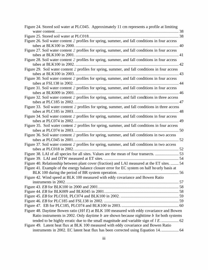
Figure 7. Aerial photograph and EC, soil water and LAI measurement locations at EC site PLC074. ................................................................................................................................ 11
Figure 8. Aerial photograph and EC, soil water and LAI measurement locations at EC site PLC185. ................................................................................................................................ 12
Figure 9. Energy balance components measured at BLK100. H calculated using air temperature measured with both fine wire thermocouple and sonic anemometer agreed well. ............... 14
Figure 10. Latent heat flux from three collocated systems at BLK 100 for September 1-3, 2000................................................................................................................................................ 18
Figure 11. Hydrosense laboratory calibration for surface measurements at BLK100................. 22 Figure 12. Hydrosense laboratory calibration for surface measurements at PLC074 (top) and
PLC185 (bottom). ................................................................................................................. 23 Figure 13. Mean daily ETr and its standard deviation (STD) estimated by the modified Penman
equation from climatic data collected at Bishop, California (CIMIS, 2003, station #35). ... 28 Figure 14. Depth to water in two test wells located near BLK100. Test well 850T is adjacent to
the EC station; 454T is located southeast of the site, adjacent to the LA Aqueduct. ........... 32 Figure 15. Depth to water in test well 586T located near BLK009. ............................................. 32 Figure 16. Depth to water in test well 485T located south of PLC045 and estimated DTW at PLC
045 by assuming the fluctuations at the two locations were similar..................................... 33 Figure 17. Depth to water in test well 746T located at FSL138. .................................................. 33 Figure 18. Depth to water from land surface in test well 12UT located at PLC074 and adjacent
well 12CT measured from reference point with water level logger. .................................... 34 Figure 19. Stored soil water at BLK100. ...................................................................................... 35 Figure 20. Stored soil water at BLK009. ...................................................................................... 36 Figure 21. Stored soil water at FSL138. ....................................................................................... 36 Figure 22. Stored soil water at PLC074........................................................................................ 37 Figure 23. Stored soil water at PLC185........................................................................................ 37
iii
Figure 24. Stored soil water at PLC045. Approximately 11 cm represents a profile at limiting water content. ........................................................................................................................ 38
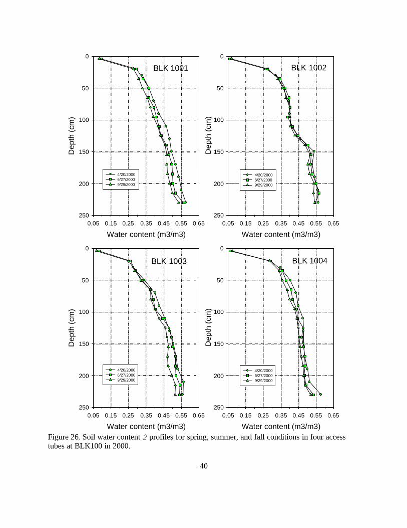
Figure 25. Stored soil water at PLC018........................................................................................ 38 Figure 26. Soil water content 2 profiles for spring, summer, and fall conditions in four access
tubes at BLK100 in 2000. ..................................................................................................... 40 Figure 27. Soil water content 2 profiles for spring, summer, and fall conditions in four access
tubes at BLK100 in 2001. ..................................................................................................... 41 Figure 28. Soil water content 2 profiles for spring, summer, and fall conditions in four access
tubes at BLK100 in 2002. ..................................................................................................... 42 Figure 29. Soil water content 2 profiles for spring, summer, and fall conditions in four access
tubes at BLK100 in 2003. ..................................................................................................... 43 Figure 30. Soil water content 2 profiles for spring, summer, and fall conditions in four access
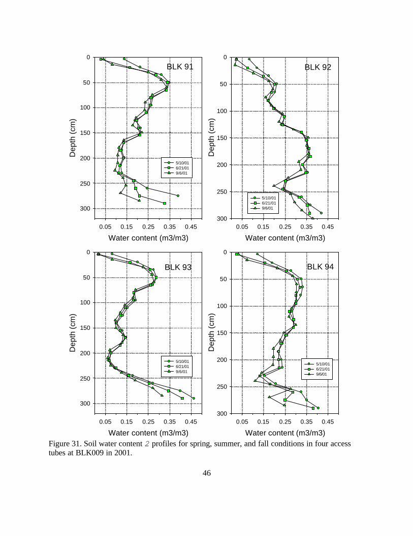
tubes at FSL138 in 2002. ...................................................................................................... 44 Figure 31. Soil water content 2 profiles for spring, summer, and fall conditions in four access
tubes at BLK009 in 2001. ..................................................................................................... 46 Figure 32. Soil water content 2 profiles for spring, summer, and fall conditions in three access
tubes at PLC185 in 2002. ...................................................................................................... 47 Figure 33. Soil water content 2 profiles for spring, summer, and fall conditions in three access
tubes at PLC185 in 2003. ...................................................................................................... 48 Figure 34. Soil water content 2 profiles for spring, summer, and fall conditions in four access
tubes at PLC074 in 2002. ...................................................................................................... 49 Figure 35. Soil water content 2 profiles for spring, summer, and fall conditions in four access
tubes at PLC074 in 2003. ...................................................................................................... 50 Figure 36. Soil water content 2 profiles for spring, summer, and fall conditions in two access
tubes at PLC045 in 2001. ...................................................................................................... 52 Figure 37. Soil water content 2 profiles for spring, summer, and fall conditions in two access
tubes at PLC018 in 2002. ...................................................................................................... 52 Figure 38. LAI of all species for all sites. Values are the mean of four transects. ....................... 53 Figure 39. LAI and DTW measured at ET sites. ......................................................................... 54 Figure 40. Relationship between plant cover (fraction) and LAI measured at the ET sites. ........ 54 Figure 41. Example of the energy balance closure error for EC system on half hourly basis at
BLK 100 during the period of BR system operation. ........................................................... 56 Figure 42. Wind speed at BLK 100 measured with eddy covariance and Bowen Ratio
instruments in 2002. .............................................................................................................. 57 Figure 43. EB for BLK100 in 2000 and 2001............................................................................... 58 Figure 44. EB for BLK009 and BLK045 in 2001......................................................................... 58 Figure 45. EB for PLC018, PLC074 and BLK100 in 2002. ......................................................... 59 Figure 46. EB for PLC185 and FSL138 in 2002. ......................................................................... 59 Figure 47. EB for PLC185, PLC074 and BLK100 in 2003. ........................................................ 60 Figure 48. Daytime Bowen ratio (H/λE) at BLK 100 measured with eddy covariance and Bowen
Ratio instruments in 2002. Only daytime β are shown because nighttime β for both systems tended to be highly erratic due to the small magnitude and variable sign of λE. ................. 62
Figure 49. Latent heat flux at BLK 100 measured with eddy covariance and Bowen Ratio instruments in 2002. EC latent heat flux has been corrected using Equation 14. ................. 64

iv
Figure 50. Half-hourly energy balance components measured at PLC185 (top graph) and BLK100 (bottom graph). ...................................................................................................... 65
Figure 51. All uncorrected ET measured by EC systems. ............................................................ 67 Figure 52. All ET corrected for energy imbalance and fitted Fourier models used for integration.
............................................................................................................................................... 67 Figure 53. λEcorr at BLK100 in 2000 measured with the EC system and TGB and TKc estimated
using measured LAI Equations 7 and 9. Fourier model fitted to λEcorr also shown. ........... 69 Figure 54. λEcorr at BLK100 in 2001 measured with the EC system and TGB and TKc. Fourier
model fitted to λEcorr also shown. ......................................................................................... 69 Figure 55. λEcorr at BLK009 in 2001 measured with the EC system and TGB and TKc. EC
measurements corrected and uncorrected for energy balance closure error are presented. Fourier model fitted to λEcorr also shown. ............................................................................ 70
Figure 56. λEcorr at PLC045 in 2001 measured with the EC system and TGB and TKc. EC measurements corrected and uncorrected for energy balance closure error are presented. Fourier model fitted to λEcorr also shown. ............................................................................ 70
Figure 57. λEcorr at BLK100 in 2002 measured with the EC system and TGB and TKc. Fourier model fitted to λEcorr also shown. ......................................................................................... 71
Figure 58. λEcorr at FSL138 in 2002 measured with the EC system and TGB and TKc. Fourier model fitted to λEcorr also shown. ......................................................................................... 71
Figure 60. λEcorr at PLC074 in 2002 measured with the EC system and TGB and TKc. Fourier model fitted to λEcorr also shown. ......................................................................................... 72
Figure 61. λEcorr at PLC185 in 2002 measured with the EC system and TGB and TKc. Fourier model fitted to λEcorr also shown. ......................................................................................... 73
Figure 62. λEcorr at BLK100 in 2003 measured with the EC system and TGB and TKc. Fourier model fitted to λEcorr also shown. ......................................................................................... 73
Figure 63. λEcorr at PLC074 in 2003 measured with the EC system and TGB and TKc. Fourier model fitted to λEcorr also shown. ......................................................................................... 74
Figure 64. λEcorr at PLC185 in 2003 measured with the EC system and TGB and TKc. Fourier model fitted to λEcorr also shown. ......................................................................................... 74
Figure 65. Predicted growing season transpiration from the Kc and GB models (shaded cells in Table 8) plotted against measured ET. PLC045 and PLC018 not plotted. .......................... 78
Figure 66. Measured LAI for dominant species, SPAI and DISP2, at BLK100 in 2000 and LAI models in TKc (Steinwand, 1998) and TGB. Measured LAI is the mean of the four transects. Measurements taken on July 7 were used to set the maximum of the LAI models.............. 81
Figure 67. Measured LAI for dominant species, SPAI and DISP2, at BLK100 in 2001 and LAI models in TKc (Steinwand, 1998) and TGB. Measured LAI is the mean of the four transects. Measurements taken on July 9 were used to set the maximum of the LAI models.............. 82
Figure 68. Measured LAI for dominant species, SPAI and CHNA2, at BLK009 in 2001 and LAI models in TKc (Steinwand, 1998) and TGB. Measured LAI is the mean of the four transects. Measurements taken on July 11 were used to set the maximum of the LAI models............ 83
Figure 69. Measured LAI for dominant species, ATTO, at PLC045 in 2001 and LAI models in TKc (Steinwand, 1998) and TGB. Measured LAI is the mean of the four transects.

v
Measurements taken on July 9 were used to set the maximum of the LAI models. Neither model was designed to accommodate the bimodal pattern exhibited at this site.................. 84
Figure 70. Measured LAI for dominant species, SPAI and DISP2, at BLK100 in 2002 and LAI models in TKc (Steinwand, 1998) and TGB. Measured LAI is the mean of the four transects. Measurements taken on July 10 were used to set the maximum of the LAI models............ 85
Figure 71 Measured LAI for dominant species, ATTO and DISP2, at PLC074 in 2002 and LAI model in TKc (Steinwand, 1998) and TGB. Measured LAI is the mean of the four transects. Measurements taken on June 5 were used to set the maximum of the LAI models. ............ 86
Figure 72. Measured LAI for dominant species, SAVE, at PLC074 in 2002 and LAI model in TKc (Steinwand, 1998) and TGB. Measured LAI is the mean of the four transects. Measurements taken on June 5 were used to set the maximum of the LAI models. .................................... 87
Figure 73. Measured LAI for dominant species, SAVE, at PLC185 in 2002 and LAI model in TKc (Steinwand, 1998) and TGB. Measured LAI is the mean of the four transects. Measurements taken on June 5 were used to set the maximum of the LAI models. ............ 87
Figure 74. Measured LAI for dominant species, DISP2, at FSL138 in 2002 and LAI model in TKc (Steinwand, 1998) and TGB. Measured LAI is the mean of the four transects. Measurements taken on July 8 were used to set the maximum of the LAI models. ..................................... 88
Figure 75. Measured LAI for dominant species, CHNA2, at PLC018 in 2002 and LAI model in TKc (Steinwand, 1998) and TGB. Measured LAI is the mean of the four transects. Measurements taken on July 8 were used to set the maximum of the LAI models.............. 88
Figure 76. Measured LAI for dominant species, SPAI and DISP2, at BLK100 in 2003 and LAI models in TKc (Steinwand, 1998) and TGB. Measured LAI is the mean of the four transects. Measurements taken on July 14 were used to set the maximum of the LAI models............ 89
Figure 77. Measured LAI for dominant species, ATTO and DISP2, at PLC074 in 2003 and LAI model in TKc (Steinwand, 1998) and TGB. Measured LAI is the mean of the four transects. Measurements taken on June 9 were used to set the maximum of the Kc LAI models and July 15 for GB models .......................................................................................................... 90
Figure 78. Measured LAI for dominant species, SAVE, at PLC074 in 2003 and LAI model in TKc (Steinwand, 1998) and TGB. Measured LAI is the mean of the four transects. Measurements taken on June 9 were used to set the maximum of the Kc LAI models and July 15 for GB models ................................................................................................................................... 91
Figure 79. Measured LAI for dominant species, SAVE, at PLC185 in 2003 and LAI model in TKc (Steinwand, 1998) and TGB. Measured LAI is the mean of the four transects. Measurements taken on June 10 were used to set the maximum of the Kc LAI models and July 15 for GB models .......................................................................................................... 91
Figure 80. Mean daily ETr and daily ETr measured in 2000-2002 at the CIMIS station in Bishop, Ca. ......................................................................................................................................... 92

vi
LIST OF TABLES Table 1. Eddy covariance site characteristics. Depth to water change during the growing season
is given, and precipitation values are annual totals beginning October 1 the previous year. . 5 Table 2. Dates of EC station operation. ....................................................................................... 13 Table3. Statistics of EC tower comparison at BLK100. .............................................................. 19 Table 4. Date for maximum measured LAI for the dominant species and dates of maximum LAI
in the Green Book and Kc models (LAIj in the GB model is July 5 (DOY 186) for all species). LAI sampling dates used to for TKc and TGB calculation are listed in the last column. .................................................................................................................................. 26
Table 5. Estimated model parameters for standardized mean daily ETr series for 1983-2001 in Bishop, California. Data are from CIMIS Station #35). ...................................................... 30
Table 6. ETcorr Fourier model coefficients and r2 for each site-year............................................ 68 Table 7. RMSE between eddy covariance ET corrected for energy balance closure and T
estimated from Kc and GB models. ...................................................................................... 76 Table 8. Eddy covariance ET corrected for energy balance closure and T model predictions. LAI
data collected in early June and July (before and after the solstice) were used to bracket the Kc and GB model predictions of T. TKc relied on mean daily ETr. Measured and predicted fluxes are the sum of daily totals extrapolated for the growing season (March 25 to October 15). ........................................................................................................................................ 77

1
EXECUTIVE SUMMARY
In 2000, Inyo County and LADWP began a cooperative study designed to compare
methods of forecasting plant water requirements based on vegetation leaf area with independent
micrometerological measurements of evapotranspiration (ET). Towers equipped with eddy
covariance (EC) sensors to measure the vertical flux of heat and water vapor were installed at
seven sites over four growing seasons. As in other studies using the EC technique, the amount of
energy accounted for by heat flow and evaporation was less than total available energy. To
address this discrepancy, an additional experiment comparing results from Bowen ratio and EC
stations was successfully completed to develop a procedure to adjust the EC measurements.
Two transpiration models to determine plant water requirements, the current Green Book
(GB) method and a similar method based on transpiration coefficients (Kc), were compared with
measured ET. The GB and Kc models best agreed with measured values of ET for essentially
equal numbers of site-years, but the Kc model and its leaf area component performed marginally
better than the GB model. The preferred transpiration model for management could not be
determined, however, as both models tended to underestimate growing season ET. Failure to
identify the superior model was partially due to the narrow range of site conditions that meet
assumptions in the models and also due to the small difference between the models relative to the
precision of the ET measurement. Often neither model predicted ET well and average deviation
from measured ET was relatively large, approximately 8 to 9 cm over the growing season,
despite the attempt to select sites that met the assumptions of the transpiration models. Reliance
on forecasted plant water requirements for groundwater management is not advised without
provisions to consider the potentially large error in the forecasts.

2
Introduction
Pumping is managed under the Inyo/Los Angeles Water Agreement (Agreement) based
on data collected at permanent monitoring sites located in wellfield areas throughout the Owens
Valley. Operational status of Los Angeles Department of Water and Power (LADWP) pumping
wells near the permanent monitoring sites is determined by comparing predicted transpiration
with the amount of plant-available soil water stored in the root zone. The transpiration
predictions are derived from vegetation measurements and functions that describe the seasonal
trends in transpiration per leaf area and leaf area index (LAI). Details of the measurement
methods and models are contained in a technical appendix to the Agreement titled the Green
Book (GB). An alternative method to prepare the transpiration predictions based on empirically-
derived transpiration coefficients (Kc) has been proposed for adoption to revise the Green Book
(Steinwand et al., 2001; Steinwand, 1999b). Both the Kc and GB methods were developed from
similar field measurements and involve scaling up from measurements made on individual leaves
or small branches to the scale of the monitoring sites. Relying on computations involving
variables measured at small scales to make large-scale forecasts requires verification against
concurrent measurements made at larger spatial scales.
There are several methods of measuring evapotranspiration (ET) using
micrometeorological measurements (Brutsaert, 1982; Shuttleworth, 1993). All such methods
measure variables near the land surface (i.e., a few meters above the plant canopy) to determine
fluxes of energy, momentum, or trace gases. The eddy covariance (EC) method has gained
predominance among micrometeorological methods recently because of its minimal theoretical
assumptions and improved instrumentation (Shuttleworth, 1993). An advantage of the eddy

3
covariance method is that it is the most direct measurement of sensible and latent heat fluxes that
is possible with micrometeorological methods. Previous studies in the Owens Valley have used
micrometeorological methods to measure water vapor fluxes from phreatophytic vegetation
(Duell, 1990; Gay, 1992; Duell, 1992), but these measurements were not made concurrently with
the necessary vegetation cover or leaf area measurements to perform a comparison with the GB
or Kc vegetation-based transpiration models.
Since 2000, Inyo County and LADWP have jointly conducted a cooperative study
entitled “Evapotranspiration (ET) from groundwater dependent plant communities: Comparison
of micrometeorological and vegetation-based measurements”. The purpose of the study is to
measure ET from groundwater dependent plant communities in the Owens Valley using EC
methods, and to compare those measurements with plant leaf area based methods of forecasting
plant water requirements. In 2002, Inyo County received funding from California Department of
Water Resources to purchase and operate two additional EC stations. Because of the similar
study design, data from sites equipped with those instruments are included in this report.
Materials and Methods
Site selection
Sites were selected based on plant species composition, depth to the water table, site
security, and fetch. Eddy covariance stations were placed in both mixed and monocultural sites
ranging from alkali meadow to scrub vegetation communities. Except for one site (PLC018), the
intent was to select sites with DTW sufficient to subirrigate the vegetation, but deep enough to
4
Upwind fetch (m)
0 50 100 150 200
Fra
ctio
n of
ET
orig
inat
ing
with
in u
pwin
d fe
tch
0.0
0.1
0.2
0.3
0.4
0.5
0.6
0.7
0.8
0.9
1.0
z=2; h=1.5 z=2; h=1.0 z=2; h=0.5 z=2; h=0.25 z=1; h=0.5 z=1; h=0.25
Figure 1. Approximate contributing area upwind of an eddy-covariance station in unstable conditions according to Gash (1986). Reasonable values were assumed for roughness height, stability, wind speed, and zero-plane displacement. z is instrument height and h is canopy height.
minimize surface evaporation. Bare soil evaporation must be minimal to allow comparison of
eddy covariance results (ET) with vegetation based estimates of transpiration (T). Soil water and
water table measurements were included in this study to examine how well these assumptions
were met. Sites PLC018 and PLC045 were typical of abandoned farmland on sandy soils and
relatively deep water tables near Bishop that are now vegetated with near-monocultures of
rabbitbrush or saltbush. Although probably not appropriate to compare to GB or Kc models,

5
Table 1. Eddy covariance site characteristics. Depth to water change during the growing season is given, and precipitation values are annual totals beginning October 1 the previous year. Year Site Vegetation type Dominant Species^ Depth to water Precipitation (m) (mm) 2000 BLK100 alkali meadow SPAI, DISP2 2.0-2.5 35.6 2001 BLK100 alkali meadow SPAI, DISP2 2.2-3.0 71.1 BLK009 Rabbitbrush meadow CHNA2, SPAI 2.6-3.2 71.1 PLC045 Nev.saltbush scrub ATTO 3.8-4.1(est.) 105.9 2002 BLK100 alkali meadow SPAI, DISP2 2.3-3.2 32.5 FSL138 alkali meadow DISP2, LETR, SPAI 1.2-2.1 21.8 PLC018 Rabbitbrush scrub CHNA2 >5.0 34.5 PLC074 Nev. saltbush
meadow SAVE4, ATTO, DISP2
2.1-2.4 31.5
PLC185 desert sink scrub SAVE4 4.0 31.5 2003 BLK100 alkali meadow SPAI, DISP2 2.1-3.3 301.8 PLC074 Nev. saltbush
meadow SAVE4, ATTO, DISP2
2.1-2.4 91.7
PLC185 desert sink scrub SAVE4 >4.0 150.9 ^: grasses: SPAI, Sporobolus airoides; DISP2, Distichlis spicata; LETR5, Leymus triticoides. shrubs: CHNA2, Chysothamnus nauseosus; ATTO Atriplex lentiformis ssp. torreyi; SAVE4, Sarcobatus vermiculatus. The rabbitbrush subspecies at PLC018 may be hololeuca.
EC data from those sites were valuable to interpret results from other sites and may be useful for
groundwater modeling efforts in another cooperative study. Methods in Gash (1986) were used
to estimate the size of the potential area contributing to the EC measurements to guide selection
of sites (Figure 1). Sites with obvious boundaries between dissimilar vegetation and hydrologic
conditions within approximately 150 m of the site were avoided. All sites were undisturbed by
water spreading or irrigation.
Locations of the EC sites are shown on Figures 2 to 8, and environmental characteristics
of the sites are summarized in Table 1. Each EC tower was fenced to prevent cattle from
damaging the instruments. The fenced exclosure at BLK100 was expanded in 2001 to include
the vegetation transects because of observed grazing impacts adjacent to the tower exclosure late
in the growing season and over winter. Cattle were not excluded from the vegetation transects at

6
Figure 2. Aerial photograph and ET, soil water, and LAI measurement locations at EC site BLK100.

7
Figure 3. Aerial photograph and EC, soil water and LAI measurement locations at EC site BLK009.

8
Figure 4. Aerial photograph and EC, soil water and LAI measurement locations at EC site PLC045.

9
Figure 5. Aerial photograph and EC, soil water and LAI measurement locations at EC site FSL138.

10
Figure 6. Aerial photograph and EC, soil water and LAI measurement locations at EC site PLC018.
11
Figure 7. Aerial photograph and EC, soil water and LAI measurement locations at EC site PLC074.

12
Figure 8. Aerial photograph and EC, soil water and LAI measurement locations at EC site PLC185.

13
Table 2. Dates of EC station operation. Year Site Date established Date removed 2000 BLK 100 April 21 January 8, 2001 2001 BLK 100 March 7 November 27 BLK 9 April 11 November 27 PLC 45 April 10 November 27 2002 BLK 100 March 12 October 2 FSL 138 May 3 September 11 PLC 18 May 2 October 8 PLC 74 May 25 October 7 PLC 185 May 24 October 7 2003 BLK 100 April 23 December 26 PLC 74 April 24 November 17 PLC 185 April 24 January 6, 2004
any other site. Three sites monitored in 2002, BLK100, PLC074 and PLC185,were also
instrumented in 2003 partly to determine if ET and the soil water balance differed after a much
wetter winter. Precipitation preceding the growing seasons each year 2000-2002 consisted of
small events, and total precipitation was below normal (about 130 mm) in all years.
Precipitation preceding the 2003 growing season was 3 to 5 times that in previous years (Table
1). In all years, EC measurements were collected during most of the growing season,
approximately March 25 to October 15 (Table 2).
Eddy covariance theory and instrumentation
The EC method of measuring turbulent fluxes uses fast-response sensors to measure rapid
changes in vertical wind speed and scalar quantities (e.g. water vapor density or heat content)
to compute the flux of the scalar by means of the covariance of the vertical wind and the scalar
(Arya, 2001). The latent heat flux is,
'' vwE ρλλ = (1)

14
April 26, 2000
Ene
rgy
flux
(W m
-2)
-100
0
100
200
300
400
500
600Latent heat fluxSensible heat flux (sonic)Sensible heat flux (thermocouple)Net radiationSoil heat flux #1Soil heat flux #2
6:00 PDT 12:00 PDT 18:00 PDT
Figure 9. Energy balance components measured at BLK100. H calculated using air temperature measured with both fine wire thermocouple and sonic anemometer agreed well.
and the sensible heat flux is,
''TwCH pρ= (2)
where λ is the latent heat of evaporation (J kg-1), w is the vertical wind speed (m s-1), ρv is the
water vapor density (kg m-3), ρ is the mean air density (kg m-3), Cp is the specific heat of air (J
kg-1 K-1), T is the air temperature. Primes indicate deviations from the time-averaged mean, and
the overbar indicates time averaging.

15
Vertical wind speed was measured with a Campbell CSAT sonic anemometer (Campbell
Scientific Inc., 1998a), the water vapor density was measured with a Campbell KH20 krypton
hygrometer (Campbell Scientific Inc., 1989), and air temperature was measured using a fine-wire
thermocouple, all of which were mounted 2.5 m above the land surface. Sensible heat flux was
calculated using both the temperature as calculated from the sonic anemometer and as measured
by the fine wire thermocouple, and the two methods had close agreement at BLK100 (Figure 9).
The fine wire thermocouples were replaced repeatedly due to breakage which resulted in an
intermittent record; therefore, the sonic temperature was used in computing the sensible heat
flux. The data were acquired and the covariance computed at 10 Hz, and fluxes were averaged
over 30 minute intervals. The EC system has the advantage that the computed covariance
theoretically provides a direct measure of the scalar flux at the point of measurement.
Difficulties in the EC method arise in the demands made on the instrumentation to acquire data
at the necessarily rapid sampling rate, and the fact that the measurements in practice are non-
collocated volume averages rather than collocated at a point as assumed by Equations 1 and 2.
The EC measurements were corrected for absorption of the krypton hygrometer
ultraviolet beam by oxygen (Campbell Scientific Inc., 1998b), and for the effect of fluctuating air
density (Webb et al., 1980). These corrections were implemented as,
++=
TkHFk
TCH
wEwp
vv
0''ρρ
ρλλ (3)
where F is a factor to account for the fraction of oxygen in air (gm K J-1), ko is the oxygen
absorption coefficient (0.0045 m3 gm-1 cm-1), and kw is the water vapor absorption coefficient
(0.154 m3 gm-1 cm-1). The first term in the parentheses is the uncorrected EC vapor flux, the

16
second term corrects for fluctuations in air density, and the third term corrects for the effect of
oxygen on the krypton hygrometer.
Though not necessary to make the EC measurement of turbulent fluxes, the EC systems
were also equipped with a REBS Q-7.1 net radiometer (Campbell Scientific Inc., 1996), soil heat
flux plates (Campbell Scientific Inc., 1999), soil temperature sensors, and a frequency domain
reflectometer (Campbell Scientific Inc., 1996) for measuring soil wetness. These additional
instruments allow the energy balance to be computed. Two soil heat flux plates were installed at
a depth of 8 cm approximately 1 m apart, and soil temperature thermocouples were installed at
depths of 2 and 6 cm between the flux plates. The soil heat flux at the soil surface was computed
by correcting the heat flux measured at the flux plate for thermal storage in the soil above the
flux plates,
( )sbwvwz CCtT
zGG ρρθ +∆∆
∆+= (4)
where Gz is the average of the two flux plates (W m-2), ∆z is the depth of the flux plates, ∆T is
the average change in temperature of the two soil temperature thermocouples (Co), ∆t is the time
interval over which the flux is averaged (s), Cw is the specific heat capacity of water (4.18 J g-1
K-1), θv is the volumetric soil water content, ρw is the density of water (1.00 gm cm-3), ρb is the
measured soil bulk density (1.11 gm cm-3), and Cs is the specific heat capacity of dry soil
material (0.87 J gm-1 K-1). Soil bulk density was determined by oven drying soil samples, water
content was measured by FDR, and the specific heat capacity of dry soil material was taken from
Campbell and Norman, Table 8.2 (1998). The sign convention adopted throughout this report is:
net radiation is positive when directed toward the land surface, sensible and latent heat fluxes are

17
positive when directed away from the land surface, and soil heat flux is positive when directed
into the soil.
Several quality control measures were implemented to ensure accurate data were
collected. The towers were instrumented to measure all components of the energy balance (EB)
to allow an independent check of the ET measured by the EC methods using,
EHGRnEB λ−−−= (5)
where Rn is net radiation (W m-2), H, G, and λE as defined above. EB should equal zero if
canopy heat storage, photosynthetic absorption of solar radiation, and advective energy transport
processes are negligible. EC measurements collected during this study and others (Bidlake,
2000; Bidlake 2002; Norman and Baker, 2002; Berger et al., 2001; Sumner, 1996; Stannard,
1993) have found that EB does not equal zero, with the sum of the turbulent fluxes (H + λE)
measured by the EC instruments generally being less than the available energy (Rn − G). Results
of the analysis of EB are described more fully in a separate section below.
Post processing of the EC data included inspection of the record for anomalies in all data
streams and inspection of the turbulent flux data for sonic anemometer spikes or signal losses. If
more than 5% of the 10 Hz signal from the eddy covariance sensors was lost over a thirty-minute
sampling interval, that interval was discarded. Routine maintenance and data downloads were
done during each site visit at roughly weekly intervals. Typically, the data were downloaded, the
windows on the hygrometer were cleaned, the net radiometer domes were cleaned, the sonic
anemometer and net radiometer were checked for level, the solar panel was cleaned, and sensor
output was examined to make sure all sensors were recording correctly. Upon the completion of

18
2000
late
nt h
eat f
lux,
W m
-2
-50
0
50
100
150
tower 1tower 2tower 3
Sept 1 Sept 2 Sept 3
Figure 10. Latent heat flux from three collocated systems at BLK 100 for September 1-3, 2000.
measurements each year, the EC instruments were removed from the field for factory
recalibration.
For 62 days during July to October, 2000, three EC systems were installed at BLK100 to
collect concurrent ET, air temperature, and humidity measurements. For this comparison, the
instrument towers were placed about 4 meters apart, arrayed roughly perpendicular to the mean
wind direction. The most significant data gaps are in the net radiation record, which lost data
during the interval from day of year (DOY) 119 to 130 due to a problem with the datalogger
program, from DOY 177 to 180 due to rodents chewing through the instrument cable, and from
DOY 284 though 294 due to a broken radiometer dome. All three systems were powered down

19
Table3. Statistics of EC tower comparison at BLK100. Tower 1 Tower 2 Tower 3 mean LE flux (W m-2) 32.87 34.26 33.89 standard deviation 47.03 48.61 48.36 % of mean of all towers (33.67 W m-2) 97.6% 101.7% 100.6%
and instruments removed from the field during the period DOY 242 through 245 due to
inclement weather. Short intervals of data were lost when the transducer heads of the sonic
anemometer were wet due to rain. Simultaneous operation of three collocated eddy covariance
systems showed that latent heat fluxes measured by the three systems agreed within a few
percent of with one another (Figure 10). Table 3 compares the statistics of the latent heat fluxes
measured by each system.
The ET record at all sites contained gaps due to instrument failure, or the record was
truncated before the end or after the beginning of the growing season. To provide uniform limits
for integration and to permit site to site comparisons and year to year comparisons, the EC data
were fit to a Fourier model like that used to predict reference ET (ETr, described below). This
model was chosen because of its demonstrated ability to model the seasonal changes in
evaporative demand represented by ETr (Or and Groeneveld, 1994). Occasionally the fitted
model was poorly constrained during winter when EC data were lacking and gave negative
values. When this occurred, daily ET was assumed to be 0.01 mm day-1 and the model was
revised. This procedure was largely for graphical purposes, and the effect on the comparison
with Kc and GB transpiration models was negligible because only the daily ET or T values
during the growing season were summed.
20
Bowen ratio theory and instruments
Energy fluxes measured by the EC system were compared to fluxes measured with a
Bowen ratio (BR) system to examine the EB closure problem and to develop recommendations
for processing the EC data to estimate λE. A BR system was installed and operated by Dr. Jim
Stroh of Evergreen State College from August 23 to September 3, 2002 at BLK100 adjacent to
the EC tower. The instrument towers were located 5 m apart in an east-west alignment so wakes
on the lee side of each tower would not interfere with the other tower during the prevailing
afternoon southeasterly winds. The net radiometers were mounted 5 m apart and 3 m south of
their respective instrument towers.
The BR method relies on different assumptions and instrumentation than EC to estimate
fluxes. Agreement between the two methods would strongly corroborate the results, and
disagreement between the methods can help determine likely sources of error. The BR
method uses measurements of water vapor density and temperature at two heights to compute the
average gradients near the surface, and then by equating the eddy diffusivity for sensible and
latent heat, uses Equation 5 and the measured Bowen ratio (β = H/λE) to compute the turbulent
fluxes. Beyond its use in the BR method, β is significant as a measure of the relative partitioning
of available energy between sensible and latent heat. The BR system consisted of fine wire
thermocouples mounted at 1.0 and 2.0 m above the surface, a chilled mirror hygrometer, an air
pump and routing system that alternately directs an air stream from the upper and lower sensor
arms to the hygrometer, a net radiometer, soil heat flux plates, and soil temperature sensors.
Fluxes were averaged over 20 minute intervals. The BR method has the advantage that the
instrumentation is relatively simple compared to the EC method, but has the disadvantage that

21
energy balance is used to compute the fluxes. The energy balance cannot be used as a check on
the internal consistency of the computed fluxes, and any errors in measuring available energy
affect the computation of the turbulent fluxes. The chilled mirror hygrometer has a limited range
of environmental conditions under which it will function properly. In very dry conditions, ve ry
warm conditions, or very cool conditions, formation of frost on the mirror surface confounds the
dew point measurement. The early fall season was chosen for operation of the BR system at this
site because it was expected that conditions would be within the applicable range of the chilled
mirror hygrometer. Soil heat flux was computed as described for the EC systems.
Two sources of error that are common to both BR and EC measurements are the
mismatch between the sampling areas ("footprints") of the various sensors used to compute
fluxes and energy balances, and the variability of the landscape within the footprint. For
example, the sonic anemometer and krypton hygrometer combine to sense water vapor flux
integrated over a footprint with a radius on the order of 100 m, whereas the calculation of soil
heat flux has a footprint of about a square meter. Similar mismatches of measurement areas or
volumes are present in the BR instrumentation. Because the land surface properties that affect
the energy balance are spatially heterogeneous, these footprint mismatches limit the precision
with which the energy balance at a point can be estimated.
Soil water, groundwater, and precipitation measurements
Detailed measurements of soil water content were conducted using a combination of time
domain reflectometry (TDR), neutron gauge , and gravimetric sampling. Soil depths 20 cm and
below were monitored in 15 cm increments using a neutron gauge. Three or four access tubes
were installed adjacent to the vegetation transects and usually to the water table. Only one

22
Hydrosense Period (ms)
0.8 1.0 1.2 1.4 1.6
Wat
er C
onte
nt (
m3 m
-3)
0.0
0.1
0.2
0.3
0.4
0.5
0.6
0.7
MeasurementRegression
y = -1.69+2.82x-0.87x2
r2 = 0.99
Figure 11. Hydrosense laboratory calibration for surface measurements at BLK100.
access tube extended to depths below one meter at PLC045 because augered holes in the dry,
sandy soil collapsed repeatedly. Access tubes were constructed of PVC except at PLC018 where
aluminum tubes were used. The neutron gauge was calibrated by regressing volumetric water
content (2) of soil samples collected during access tube installation at each site against neutron
gauge count ratio (count/field standard count) recorded at the sampling depths. Determination of
2 followed Blake and Hartage (1986). Soil cores of a known volume were collected, weighed,
and dried at 105 oC for 24 hours to determine the gravimetric water content (g water/g soil) and
bulk density (g soil cm-3 soil). Volumetric water content (cm3 water/cm3 soil) is the product of
gravimetric water content and bulk density (assuming the density of water is 1 g cm-3). Shallow

23
Hydrosense Period (ms)
0.80 0.85 0.90 0.95 1.00 1.05
Wat
er c
onte
nt (
m3 m
-3)
0.00
0.05
0.10
0.15
0.20
0.25
0.30
0.35
0.40
0.45
MeasurementRegression
Hydrosense Period (ms)
0.80 0.85 0.90 0.95 1.00 1.05
Wat
er c
onte
nt (
m3
m-3
)
0.00
0.05
0.10
0.15
0.20
0.25
0.30
0.35
0.40
0.45
MeasurementRegression
y = -3.93 + 7.59x-3.40x2
r2 = 0.99
y = -2.92 + 2.72xr2 = 0.99
Figure 12. Hydrosense laboratory calibration for surface measurements at PLC074 (top) and PLC185 (bottom).

24
depths were monitored using gravimetric sampling (0-8 cm) or TDR. Surface TDR
measurements are less destructive and quicker than gravimetric samples prompting the change in
methods in 2003. Surface (0-12 cm) measurements were collected using a Hydrosense™ TDR
system using site-specific calibrations prepared in the laboratory by gradual drying of soil with
embedded TDR probes (Steinwand and Olsen, 2003). Linear or quadratic models were fit to
data consisting of paired measurements of TDR period and volumetric soil water content
(Figures 11 and 12). In the field, the instrument was most reliable at sites with dry sandy soils
(PLC074, PLC185) and least reliable at BLK100 when the soil was moist probably due to soil
salinity interference with the built in algorithm to interpret the TDR signal. Gravimetric samples
were collected when the TDR failed. Soil water was measured biweekly during the growing
season and approximately monthly in winter.
Soil water stored in the entire monitoring depth (cm H2O/soil depth) was calculated
according to,
iitube zStorage ∆= ∑θ (6)
where 2i is volumetric water content at depth i and )zi is the thickness of the soil interval
represented by 2i. Existing on-site test wells were monitored at FSL138, PLC074, BLK009, and
BLK100 (beginning in February, 2001). Depth to water (DTW) in nearby test wells was
monitored at PLC045, and BLK100 (before February, 2001). Sites PLC018 and PLC185 were
not located near test wells. Water level loggers were installed in test wells at BLK100 and
PLC074 in June and July, 2003 respectively, to replace manual measurements. Precipitation was
measured after each event by Inyo County or daily by the National Oceanic and Atmospheric
Administration (NOAA) (Table 1). Rain gauges assigned to the sites were: Inyo County RG-6:

25
BLK100, BLK009; Bishop Airport NOAA: PLC045, PLC018; Inyo County RG-3: PLC074,
PLC185; Inyo County RG-1: FSL138.
Vegetation measurements
Four 50 m vegetation transects aligned approximately north, south, east, and west of the
EC station exclosures were established at each site. Point frame measurements with 50 cm pin
spacing were conducted approximately monthly during the growing season (approximately
March through October), and first contacts and all contacts with green live, green leaves or stems
were recorded by species to determine plant cover and leaf area index (LAI) (Goodall, 1952).
Plant cover was calculated as the fraction of pins tha t contacted at least one green leaf or stem.
Contact frequency (total contacts ) total pins) was used to calculate LAI according to,
KN
LAI = (7)
where N is contact frequency for a species and K is an extinction coefficient determined
empirically for common Owens Valley species (Groeneveld, 1997). Extinction coefficients for
species not examined by Groeneveld (1997) were assigned a value of 0.5 which was
approximately the average value for common species.
Transpiration models
Two methods based on vegetation measurements were used to estimate transpiration to
compare with the EC measurements. One method followed the procedures and models in the
Green Book, section III. The second method utilized transpiration coefficients presented in
Steinwand et al. (2001) and Steinwand (1999b). Both models were developed from porometric
methods and assume soil water conditions are not limiting. Growing seasonal totals were daily
values summed for the period March 25 to October 15.

26
Table 4. Date for maximum measured LAI for the dominant species and dates of maximum LAI in the Green Book and Kc models (LAIj in the GB model is July 5 (DOY 186) for all species). LAI sampling dates used to for TKc and TGB calculation are listed in the last column. Year Site Dominant
species^ Date of maximum LAI measured in this study
Kc LAI model maximum DOY
LAI Sampling dates for TGB and TKc calculation
2000 BLK 100 SPAI, DISP2 July 7, Sept. 7 July 20, July 8 June 7 & July 7 2001 BLK 100 SPAI, DISP2 Sept. 9, Aug. 8 July 20, July 8 June 12 & July 9 BLK 9 CHNA2, SPAI May 15, June 14 July 3, July 20 June 14 & July 11 PLC 45 ATTO June 11 June 12 June 11 & July 9 2002 BLK 100 SPAI, DISP2 Aug. 5, June 3 July 20, July 8 June 3 & July 10 FSL 138 DISP2,
LETR5, JUBA July 9 (DISP2) July 8 June 3 & July 9
PLC 18 CHNA2 June 3 July 3 June 3 & July 9 PLC 74 SAVE4,
ATTO, DISP2 June 5, June 5, July 5 June 23, June
12, July 8 June 5 & July 5
PLC 185 SAVE4 May 8 June 23 June 5 & July 5 2003 BLK 100 SPAI, DISP2 Sept. 9 July 20, July 8 June 3 & July 14 PLC 74 SAVE4,
ATTO, DISP2 June 9 June 23, June
12, July 8 June 9 & July 15
PLC 185 SAVE4 May 9 June 23 June 10 & July 14 ^: grasses; SPAI, Sporobolus airoides; DISP2, Distichlis spicata; LETR5, Leymus triticoides. shrubs; JUBA, Juncus balticus: CHNA2, Chysothamnus nauseosus; ATTO Atriplex lentiformis ssp. torreyi; SAVE4, Sarcobatus vermiculatus.
The model contained in the Green Book to predict T is,
))(( 22103000
)186(
1 1
2
iiLAIT jjj
i
j
n
j
m
iGB e βββ ++=
−−
= =∑∑ (8)
where i is day of year, LAIj is the LAI on July 5 for species j, n is number of species, $0, $1, and
$2 are coefficients of a polynomial model fit to porometric measurements of transpiration per
leaf area for each species (Green Book, Table III.D.1.c). Constants in the exponential model
were based on the assumed progression of LAI during the year.
Transpiration coefficients are a dimensionless ratio of actual ET (in this case T) to a
reference or potential ET typically determined over an irrigated grass or alfalfa reference crop.
The general form of transpiration coefficients is,

27
ETreferenceETactual
Kc = (9)
Once the Kc for a plant species (usually a crop) is known, actual ET for another site or time can
be derived from measurements of reference ET by rearranging Equation 9. The ratio in Equation
9 is a general concept, and transpiration coefficients take several forms including modifications
for growing season weather, time-varying leaf area/canopy closure, or irrigation (Allen et al.,
1998). The particular form of the Kc can be tailored to specific situations as long as its
application is consistent with the definition and assumptions used to develop the coefficient.
Transpiration coefficients from Steinwand (1999b) and Steinwand et al. (2001), measured LAI ,
and mean daily reference ET were used to calculate TKc as,
)(1 1
ji
n
j
m
iijKc LAIETrKcT ∑∑
= =
= (10)
where i is DOY, ETri is mean daily reference ET, n is number of species, Kcij is the transpiration
coefficient for species j, LAIj is the midsummer LAI for species j. The Kc models were
developed from a large database of porometric measurements of stomatal conductance, reference
ET, and LAI for the five most common Owens Valley species.
Models of seasonal trends in LAI were included in TKc and TGB to allow use of a single
LAI measurement at the peak of the growing season to provide site-specific estimates of
transpiration. Changes in LAI during the growing season were incorporated directly into TGB by
assuming the seasonal trend follows the Gaussian model in Equation 8. In contrast, seasonal
LAI trends were incorporated during the construction of Kcij in Equation 10 by relying on

28
Figure 13. Mean daily ETr and its standard deviation (STD) estimated by the modified Penman equation from climatic data collected at Bishop, California (CIMIS, 2003, station #35).
models of daily LAI fit to existing data and normalized to a maximum LAI of 1.0. The Green
Book model fixes the peak LAI at day of year DOY 186 (July 5). The peak LAI in the Kc
models varies by species but is in June or July (Table 4). LAI measurements in this study
typically were collected in early June and early July bracketing the maximum LAI in TKc and
TGB models. Calculations using both June and July field data were prepared in this study, but the
comparison of transpiration totals relied on the LAI data collected nearest the date of maximum
LAI in the models (Table 4). LAI of minor species for which no Kc or Green Book polynomial
models were available was apportioned among the known species based on their relative
proportion of total LAI.

29
TKc can be used to estimate transpiration for a preceding period by utilizing actual ETri
measurements (look back mode), but to predict transpiration as required by current procedures to
manage pumping requires a model of daily ETr (prediction mode) to apply Equation 10. As part
of a related study conducted by Inyo County, a stochastic model for generating mean ETri
sequences for the Owens Valley was estimated from a 19 year (1983-2001) sequence of
observations collected at Bishop (CIMIS 2003). The procedure was identical to that of a
previous cooperative study (Or and Groeneveld, 1994) except a longer data record was used.
CIMIS uses a modified Penman equation to compute ETri, from which mean ETri and a
corresponding standard deviation were obtained. A clear seasonal trend existed in the ETri time
series which was removed prior to fitting a stochastic model (Figure 13). A Fourier series was
fitted to ETri using procedures described by Salas et al., (1980). The first two harmonics of the
Fourier series are,
∑ )365
ij2( B(j) + )
365ij2
( A(j) + >ETr< = ETr2
1=j
iππ
SINCOS (11)
where i is the day of year, <ETr> is mean daily ETr for the entire year (4.12 mm/day), A(1)=-
2.73; A(2)=-0.112; B(1)=0.187; and B(2)=0.097. We used the first harmonic only because it was
capable of explaining more than 98% of the variation in average ETri indicating a strong
seasonal (periodical) trend as evident from the data.
An approach based on classical time-series analysis was adopted for fitting a stochastic
model to the residuals of mean ETri series, i.e., after removing the deterministic trend. Several
possible ARMA(p,q) stochastic models were tested based on criteria of best fit and parsimony.
Estimated parameters by the maximum likelihood method, statistics, and tests of the residuals are
given in Table 5. An ARMA(1,1) model was selected as the best model for the ETri data based

30
Table 5. Estimated model parameters for standardized mean daily ETr series for 1983-2001 in Bishop, California. Data are from CIMIS Station #35).
ARMA(p,q) Model Order
Parameters AR(1) AR(2) ARMA(1,1)
?1 0.438 0.421 0.506
?2 0.031
?1 0.085
Goodness-of-Fit and Parsimony Tests
Residuals variance s2
e 0.050 0.055 0.050
Porte Manteau
Test - QL=90
98.8 97.0 97.2
AIC -1088 -1086 -1087
on goodness-of- fit test results (Table 5), and capability to be reduced into a predictive model for
ETr. The ARMA(1,1) model is given by:
εεθφ i1-i11-i1i + - ETr = ETr (12)
where f1 is an autoregression parameter, 21 is a moving average parameter, and gi is a normally
distributed zero mean term with variance equal to s2e. The adequacy of the ARMA(1,1) was
also confirmed by its best- fit to the autocorrelation of ETr residuals.
We adopted a method proposed by Graupe and Krause (1973) for improving the ETri
model by transforming the ARMA(1,1) of ETri estimates which are based on measurements that
contain error into a first order autoregressive model, AR(1), of the unobservable "true" state:
u + TrE = TrE ii11+i~~ ϕ (13)

31
where ETri = ETri+v i, and s2u=s2
e[1+221-21/f1-21f1] (s2
u=0.06) An estimate of the
measurement variance is given by: s2v=s2
e[21/f1] (with s2v=0.0084).
Results and Discussion
Site characteristics
Depth to water measured at the EC sites is presented in Figures 14 to 18. Typically, the
shallowest DTW occurred in the spring (March or April) and declined to a maximum depth at
end of the growing season (October). FSL138 was an exception where maximum depth to water
in 746T occurred in late July. Water tables at all sites increased during the winter when the
vegetation was senescent. Test well 850T was installed in at BLK100 in 2001, but based on the
comparison with nearby test well 454T, DTW fluctuations were similar in all four years EC
measurements were collected. The general declining trend superimposed on the annual cycle at
BLK100 (Figure 14) was due to persistent below normal runoff conditions during this study.
Additionally, on August 11, 2003 two LADWP production wells sealed below a confining layer
and located 2015 meters from 850T were activated as part of a test to determine impacts of
pumping the deep confined aquifer on the shallow water table in the region. Because the
pumping effects must propagate through the confining layer, the drawdown at the EC site was
gradual and relatively small; approximately 15 cm by May, 2004. The water level at PLC074
declined during the growing season, but small fluctuations observed in July through September
probably corresponded with irrigation releases on pastures located west of the site. There was no
apparent affect on measured ET during periods of irrigation suggesting the fetch was acceptable.
No piezometer was located near PLC018 and PLC185. Soil water content at

32
BLK 100
Date
2000 2001 2002 2003 2004
Dep
th to
Wat
er (m
)
0
1
2
3
454T850T
Figure 14. Depth to water in two test wells located near BLK100. Test well 850T is adjacent to the EC station; 454T is located southeast of the site, adjacent to the LA Aqueduct.
Date
January 1, 2001 July 1 January 1, 2002 July 1
Dep
th to
Wat
er (
m)
0
1
2
3
4
BLK009
Figure 15. Depth to water in test well 586T located near BLK009.

33
PLC045
Date
July 1, 2000 January 1, 2001 July 1 January 1, 2002 July 1
Dep
th to
Wat
er (
m)
2.0
2.5
3.0
3.5
4.0
4.5
5.0
485TPLC045 estimated DTW
Figure 16. Depth to water in test well 485T located south of PLC045 and estimated DTW at PLC 045 by assuming the fluctuations at the two locations were similar.
Date
January 1, 2002 July 1 January 1, 2003
Dep
th to
Wat
er (
m)
0.0
0.5
1.0
1.5
2.0
2.5
FSL138
Figure 17. Depth to water in test well 746T located at FSL138.
34
Date
Apr Aug Dec Apr Aug Dec Apr
Dep
th to
wat
er (
m)
1.0
1.5
2.0
2.5
3.0
12UT manual reads12UT estimated 12CT
2002 2003
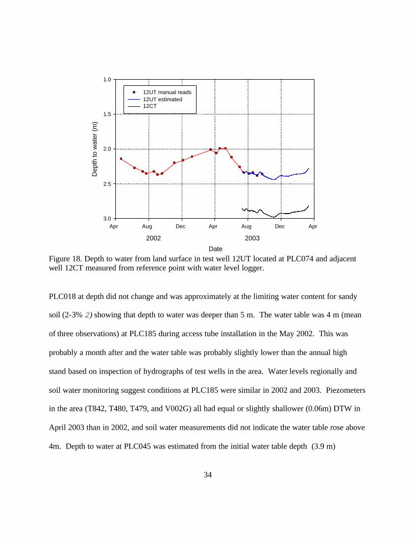
Figure 18. Depth to water from land surface in test well 12UT located at PLC074 and adjacent well 12CT measured from reference point with water level logger.
PLC018 at depth did not change and was approximately at the limiting water content for sandy
soil (2-3% 2) showing that depth to water was deeper than 5 m. The water table was 4 m (mean
of three observations) at PLC185 during access tube installation in the May 2002. This was
probably a month after and the water table was probably slightly lower than the annual high
stand based on inspection of hydrographs of test wells in the area. Water levels regionally and
soil water monitoring suggest conditions at PLC185 were similar in 2002 and 2003. Piezometers
in the area (T842, T480, T479, and V002G) all had equal or slightly shallower (0.06m) DTW in
April 2003 than in 2002, and soil water measurements did not indicate the water table rose above
4m. Depth to water at PLC045 was estimated from the initial water table depth (3.9 m)

35
DateApr 00 Oct 00 Apr 01 Oct 01 Apr 02 Oct 02 Apr 03 Oct 03
Sto
red
Soi
l Wat
er (
cm/2
.5m
)
95
100
105
110
115
120One Two Three Four Mean
Figure 19. Stored soil water at BLK100.
observed during access tube installation and fluctuations observed at a test well 485T in similar
vegetation 0.5 km southeast of the site.
Precipitation preceding the growing season each year during 2000-2002 consisted of
small events, and total precipitation was below average in all years (Table 1). Only two
summer storms in July 2001 were of significant size to affect either ET or LAI measurements,
and only at PLC045. Precipitation preceding the 2003 growing season was 3 to 5 times that in
previous years (Table 1). Summer precipitation was slightly greater in 2003 than in previous
years, but was still a small (<40mm) component of the water balance.
Soil water accumulated during winter from precipitation and groundwater recharge was
progressively depleted through the summer at all sites reflecting ET and water table decline
(Figures 19 to 25). Seasonal fluctuations were greater at sites clearly coupled to the
36
DateApr 01 Jun 01 Aug 01 Oct 01 Dec 01 Feb 02 Apr 02
Sto
red
Soi
l Wat
er (
cm/3
.0m
)
45
50
55
60
65
70
75
80
85One Two Three Four Mean
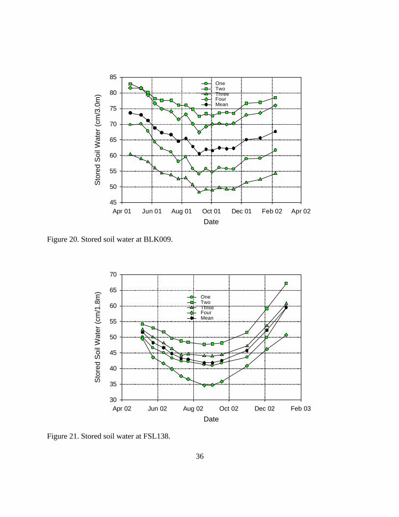
Figure 20. Stored soil water at BLK009.
DateApr 02 Jun 02 Aug 02 Oct 02 Dec 02 Feb 03
Sto
red
Soi
l Wat
er (
cm/1
.8m
)
30
35
40
45
50
55
60
65
70
One Two Three Four Mean
Figure 21. Stored soil water at FSL138.

37
Date4/1/02 7/1/02 10/1/02 1/1/03 4/1/03 7/1/03 10/1/03 1/1/04
Sto
red
Soi
l Wat
er (c
m/2
.0m
)
5
10
15
20
25
30
35
40
45
One Two Three Four Mean
Figure 22. Stored soil water at PLC074.
DateMay 02 Aug 02 Nov 02 Feb 03 May 03 Aug 03 Nov 03
Sto
red
Soi
l Wat
er (
cm/4
.0m
)
50
60
70
80
90
100One Two Three Mean
Figure 23. Stored soil water at PLC185.

38
DateApr 01 Jun 01 Aug 01 Oct 01 Dec 01 Feb 02 Apr 02
Sto
red
Soi
l Wat
er (
cm/3
.3m
)
10
11
12
13
14
15
One
Figure 24. Stored soil water at PLC045. Approximately 11 cm represents a profile at limiting water content.
DateApr 02 Jun 02 Aug 02 Oct 02 Dec 02 Feb 03
Sto
red
Soi
l Wat
er (
cm/5
.0m
)
15
16
17
18
19
20
21
One Two Mean
Figure 25. Stored soil water at PLC018.
39
water table and with higher vegetation cover (BLK100, BLK009, FSL138, PLC074). Soil water
declines during summer, 2002, were minimal at PLC045, PLC018 and PLC185 because the
small amount of winter precipitation was largely exhausted when monitoring began and because
of the weak influence of groundwater within the depth monitored. Coupling of the soil and
groundwater is discussed more fully below. Soil water storage changes at access tubes within a
site over the growing season were generally parallel suggesting that uptake/drainage was similar
and that differences in storage between tubes represented differences in soil properties,
vegetation density, or microtopography (i.e. DTW).
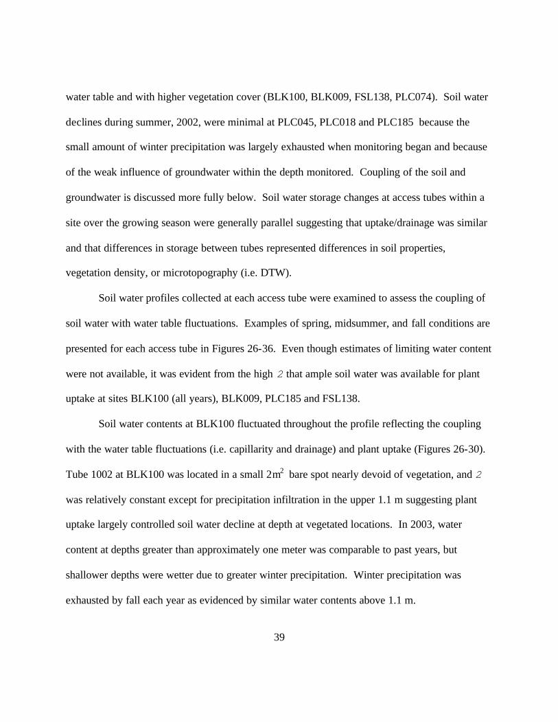
Soil water profiles collected at each access tube were examined to assess the coupling of
soil water with water table fluctuations. Examples of spring, midsummer, and fall conditions are
presented for each access tube in Figures 26-36. Even though estimates of limiting water content
were not available, it was evident from the high 2 that ample soil water was available for plant
uptake at sites BLK100 (all years), BLK009, PLC185 and FSL138.
Soil water contents at BLK100 fluctuated throughout the profile reflecting the coupling
with the water table fluctuations (i.e. capillarity and drainage) and plant uptake (Figures 26-30).
Tube 1002 at BLK100 was located in a small 2m2 bare spot nearly devoid of vegetation, and 2
was relatively constant except for precipitation infiltration in the upper 1.1 m suggesting plant
uptake largely controlled soil water decline at depth at vegetated locations. In 2003, water
content at depths greater than approximately one meter was comparable to past years, but
shallower depths were wetter due to greater winter precipitation. Winter precipitation was
exhausted by fall each year as evidenced by similar water contents above 1.1 m.
40
BLK 1001
Water content (m3/m3)0.05 0.15 0.25 0.35 0.45 0.55 0.65
Dep
th (c
m)
0
50
100
150
200
250
4/20/20006/27/2000 9/29/2000
BLK 1002
Water content (m3/m3)0.05 0.15 0.25 0.35 0.45 0.55 0.65
Dep
th (c
m)
0
50
100
150
200
250
4/20/20006/27/2000 9/29/2000
BLK 1003
Water content (m3/m3)0.05 0.15 0.25 0.35 0.45 0.55 0.65
Dep
th (c
m)
0
50
100
150
200
250
4/20/20006/27/20009/29/2000
BLK 1004
Water content (m3/m3)0.05 0.15 0.25 0.35 0.45 0.55 0.65
Dep
th (c
m)
0
50
100
150
200
250
4/20/20006/27/20009/29/2000
Figure 26. Soil water content 2 profiles for spring, summer, and fall conditions in four access tubes at BLK100 in 2000.

41
BLK 1001
Water content (m3/m3)0.05 0.15 0.25 0.35 0.45 0.55 0.65
Dep
th (c
m)
0
50
100
150
200
250
3/15/016/21/019/20/01
BLK 1002
Water content (m3/m3)0.05 0.15 0.25 0.35 0.45 0.55 0.65
Dep
th (c
m)
0
50
100
150
200
250
3/15/016/21/019/20/01
BLK 1003
Water content (m3/m3)0.05 0.15 0.25 0.35 0.45 0.55 0.65
Dep
th (c
m)
0
50
100
150
200
250
3/15/016/21/019/20/01
BLK 1004
Water content (m3/m3)0.05 0.15 0.25 0.35 0.45 0.55 0.65
Dep
th (c
m)
0
50
100
150
200
250
3/15/016/21/019/20/01
Figure 27. Soil water content 2 profiles for spring, summer, and fall conditions in four access tubes at BLK100 in 2001.

42
BLK 1001
Water content (m3/m3)0.05 0.15 0.25 0.35 0.45 0.55 0.65
Dep
th (c
m)
0
50
100
150
200
250
4/5/026/25/029/19/02
BLK 1002
Water content (m3/m3)0.05 0.15 0.25 0.35 0.45 0.55 0.65
Dep
th (c
m)
0
50
100
150
200
250
4/5/026/25/029/19/02
BLK 1003
Water content (m3/m3)0.05 0.15 0.25 0.35 0.45 0.55 0.65
Dep
th (c
m)
0
50
100
150
200
250
4/25/026/25/029/19/02
BLK 1004
Water content (m3/m3)0.05 0.15 0.25 0.35 0.45 0.55 0.65
Dep
th (c
m)
0
50
100
150
200
250
4/5/026/25/029/19/02
Figure 28. Soil water content 2 profiles for spring, summer, and fall conditions in four access tubes at BLK100 in 2002.

43
BLK 1001
Water content (m3/m3)0.05 0.15 0.25 0.35 0.45 0.55 0.65
Dep
th (c
m)
0
50
100
150
200
250
4/8/037/1/039/23/03
BLK 1002
Water content (m3/m3)0.05 0.15 0.25 0.35 0.45 0.55 0.65
Dep
th (c
m)
0
50
100
150
200
250
4/8/037/1/039/23/03
BLK 1003
Water content (m3/m3)0.05 0.15 0.25 0.35 0.45 0.55 0.65
Dep
th (c
m)
0
50
100
150
200
250
4/8/037/1/039/23/03
BLK 1004
Water content (m3/m3)0.05 0.15 0.25 0.35 0.45 0.55 0.65
Dep
th (c
m)
0
50
100
150
200
250
4/8/037/1/039/23/03
Figure 29. Soil water content 2 profiles for spring, summer, and fall conditions in four access tubes at BLK100 in 2003.

44
FSL 1381
Water content (m3/m3)0.05 0.15 0.25 0.35 0.45 0.55
Dep
th (c
m)
0
50
100
150
200
250
300
5/6/027/11/029/3/02
FSL 1382
Water content (m3/m3)0.05 0.15 0.25 0.35 0.45 0.55
Dep
th (c
m)
0
50
100
150
200
250
300
5/6/027/11/029/3/02
FSL 1383
Water content (m3/m3)0.05 0.15 0.25 0.35 0.45 0.55
Dep
th (c
m)
0
50
100
150
200
250
300
5/7/027/11/029/3/02
FSL 1384
Water content (m3/m3)0.05 0.15 0.25 0.35 0.45 0.55
Dep
th (c
m)
0
50
100
150
200
250
300
5/7/027/11/029/3/02
Figure 30. Soil water content 2 profiles for spring, summer, and fall conditions in four access tubes at FSL138 in 2002.

45
Like BLK100, FSL138 showed uptake throughout the profile above the water table
(Figure 30). Except for one location, soil water uptake largely ceased after July 11,
corresponding with reduced ET and stable or rising water table.
Vertical variation in soil water fluctuations was more complex at moist shrub dominated
sites. The soil at BLK009 can be divided into three zones based on observed soil water
fluctuations (Figure 31). Above 0.9 m, the soil was affected by infiltrating rain. Soil water
content was relatively static at intermediate depths (0.90 to 1.50-2.00 m). Below the
intermediate zone, soil water was coupled to water table fluctuations. Like BLK009, the soil at
PLC185 can be divided into three zones (Figures 32 and 33). Soil at PLC185 was dry in the
upper 1.0 m except for precipitation inputs. Intermediate depths from 1.0 m to approximately
2.7 to 3.0 m , depending on location, had nearly constant water content corresponding with
changes in soil texture. Under the drought conditions of 2002, water in this zone evidently was
not available for uptake or uptake at these depths was negligible due to low plant cover (low
rooting density). At greater depths, soil water fluctuations were coupled to water table
fluctuations, although the coupling was weak for two of the three locations. The primary plant
uptake occurred in soil above 1m and below 3.5m with a small amount of plant uptake observed
in the intermediate zone only in 2003 (e.g. tube 1853, Figure 33). PLC074 had sandy and sandy
loam soils, but the water table was relatively shallow (<3 m) and probably accessible to plant
roots. Following the dry winter in 2002, at two locations, 741 and 743, the upper 1 m was
relatively dry and decoupled from water table changes (Figure 34). At two other locations, 742
and 744, soil water content in the upper and lower profile was above limiting water content, and
it was difficult to distinguish whether the upper 1 m was coupled with the water table or whether
46
BLK 91
Water content (m3/m3)0.05 0.15 0.25 0.35 0.45
Dep
th (c
m)
0
50
100
150
200
250
300
5/10/016/21/019/6/01
BLK 92
Water content (m3/m3)0.05 0.15 0.25 0.35 0.45
Dep
th (c
m)
0
50
100
150
200
250
300
5/10/016/21/019/6/01
BLK 93
Water content (m3/m3)0.05 0.15 0.25 0.35 0.45
Dep
th (c
m)
0
50
100
150
200
250
300
5/10/016/21/019/6/01
BLK 94
Water content (m3/m3)0.05 0.15 0.25 0.35 0.45
Dep
th (c
m)
0
50
100
150
200
250
300
5/10/016/21/019/6/01
Figure 31. Soil water content 2 profiles for spring, summer, and fall conditions in four access tubes at BLK009 in 2001.

47
PLC 1851
Water content (m3/m3)0.05 0.15 0.25 0.35 0.45
Dep
th (c
m)
0
50
100
150
200
250
300
350
400
450
5/15/026/25/029/19/02
PLC 1852
Water content (m3/m3)0.05 0.15 0.25 0.35 0.45
Dep
th (c
m)
0
50
100
150
200
250
300
350
400
450
5/15/026/25/029/19/02
PLC 1853
Water content (m3/m3)0.05 0.15 0.25 0.35 0.45
Dep
th (c
m)
0
50
100
150
200
250
300
350
400
450
5/15/026/25/029/19/02
Figure 32. Soil water content 2 profiles for spring, summer, and fall conditions in three access tubes at PLC185 in 2002.

48
PLC 1851
Water content (m3/m3)0.05 0.15 0.25 0.35 0.45
Dep
th (c
m)
0
50
100
150
200
250
300
350
400
450
3/19/037/17/0310/15/03
PLC 1852
Water content (m3/m3)0.05 0.15 0.25 0.35 0.45
Dep
th (c
m)
0
50
100
150
200
250
300
350
400
450
3/19/037/17/0310/15/03
PLC 1853
Water content (m3/m3)0.05 0.15 0.25 0.35 0.45
Dep
th (c
m)
0
50
100
150
200
250
300
350
400
450
3/19/037/17/0310/15/03
Figure 33. Soil water content 2 profiles for spring, summer, and fall conditions in three access tubes at PLC185 in 2003.

49
PLC 0741
Water content (m3/m3)0.05 0.15 0.25 0.35
Dep
th (c
m)
0
50
100
150
200
5/10/026/25/029/19/02
PLC 0742
Water content (m3/m3)0.05 0.15 0.25 0.35
Dep
th (c
m)
0
50
100
150
200
5/10/026/25/029/19/02
PLC 0743
Water content (m3/m3)0.05 0.15 0.25 0.35
Dep
th (c
m)
0
50
100
150
200
5/10/026/25/029/19/02
PLC 0744
Water content (m3/m3)0.05 0.15 0.25 0.35
Dep
th (c
m)
0
50
100
150
200
5/10/026/25/029/19/02
Figure 34. Soil water content 2 profiles for spring, summer, and fall conditions in four access tubes at PLC074 in 2002.

50
PLC 0741
Water content (m3/m3)0.05 0.15 0.25 0.35
Dep
th (c
m)
0
50
100
150
200
3/19/037/3/0310/15/03
PLC 0742
Water content (m3/m3)0.05 0.15 0.25 0.35
Dep
th (c
m)
0
50
100
150
200
3/19/037/3/0310/15/03
PLC 0743
Water content (m3/m3)0.05 0.15 0.25 0.35
Dep
th (c
m)
0
50
100
150
200
3/19/037/3/0310/15/03
PLC 0744
Water content (m3/m3)0.05 0.15 0.25 0.35
Dep
th (c
m)
0
50
100
150
200
3/19/037/3/0310/15/03
Figure 35. Soil water content 2 profiles for spring, summer, and fall conditions in four access tubes at PLC074 in 2003.

51
the declines in 2 reflected uptake of precipitation-derived soil water (see below). Given the low
precipitation the preceding winter, most of the shallow soil water was probably derived from
groundwater. All access tube locations were coupled to water table fluctuations at depths below
1 to 1.5 m. In 2003, the soil at PLC074 was moist throughout the 2.0 m profile due to recharge
from the water table and deeper infiltration of winter precipitation (Figure 35). Infiltration
reached 1m in all tubes. Depths greater than 1.1m (tubes 742 and 744) to 1.4m (tubes 741 and
743) received recharge during the winter from capillarity above the water table suggesting that
the water observed above 1m in 2002 was probably derived from precipitation.
Two sites had predominately dry soils several meters thick above the water table. At
PLC045, 2 increased at depths less than 0.5-0.9 m due to winter and summer rains, but below 0.9
m, 2 was less than 0.05 m3m-3 which is approximately the limiting value for sandy loam and
sandy soils (McCuen et al., 1981). The extreme limit of capillarity above the water table (3.8 m
deep) noted during access tube installation in early spring was at 3.2 m (Figure 36). Soil at
PLC018 was dry and sandy similar to PLC045 except the limit of capillarity was below the
bottom of the access tubes, 4.7 m (Figure 37). Conditions at these sites probably violate
assumptions of sufficient soil water in the Kc and Green Book transpiration models.
LAI generally conformed to the expected seasonal trend with peak LAI occurring in early
to mid summer (Figure 38). LAI at meadow sites usually peaked in early July, approximately
one month later than shrub-dominated sites which on average exhibited maximum LAI in June.
The earlier peak leaf area of shrubs is consistent with LAI models in Steinwand (1998). The
seasonal trend at PLC045 began to decline precipitously in mid June but rebounded following

52
PLC 451
Water content (m3/m3)
0.00 0.05 0.10 0.15 0.20 0.25
Dep
th (
cm)
0
50
100
150
200
250
300
350
4/11/016/21/017/10/019/20/01
PLC 453
Water content (m3/m3)
0.00 0.05 0.10 0.15 0.20D
epth
(cm
)
0
50
100
150
200
250
300
4/11/016/21/017/10/019/20/01
Figure 36. Soil water content 2 profiles for spring, summer, and fall conditions in two access tubes at PLC045 in 2001.
PLC 0181
Water content (m3/m3)
0.00 0.05 0.10 0.15 0.20
Dep
th (
cm)
0
50
100
150
200
250
300
350
400
450
500
5/2/026/25/029/3/02
PLC 0182
Water content (m3/m3)
0.00 0.05 0.10 0.15 0.20
Dep
th (
cm)
0
50
100
150
200
250
300
350
400
450
500
5/3/026/25/029/3/02
Figure 37. Soil water content 2 profiles for spring, summer, and fall conditions in two access tubes at PLC018 in 2002.

53
Year
LAI
0.0
0.5
1.0
1.5
2.0
BLK100BLK009PLC045FSL138PLC018PLC074PLC185
20022000 2001 2003
Figure 38. LAI of all species for all sites. Values are the mean of four transects.
with PLC074 in 2002 most divergent from the overall trend (Figure 39). Total plant cover and
LAI were linearly related (Figure 40) which was expected given the linear relationship between
LAI and cover for individual species (Steinwand, 1999a and b).
Three sites were monitored multiple years. Typically, BLK100 maintained a high leaf
area through June, July, and August before declining in September (2000 and 2001) or October
(2002 and 2003). The lower in LAI in 2002 and 2003 did not correspond to construction of the
exclosure, or changes in precipitation or DTW. Leaf area trends were similar in 2002 and 2003
at PLC185 reaching a maximum in May and maintaining relatively low cover throughout the
summer. The increased LAI in May 2003 compared to 2002 was largely due to greater numbers
of short- lived annuals although SAVE4 and ATCO LAI were slightly greater as well. LAI all
species except SAVE4 increased markedly at PLC074 in 2003 probably responding to increased
winter precipitation.
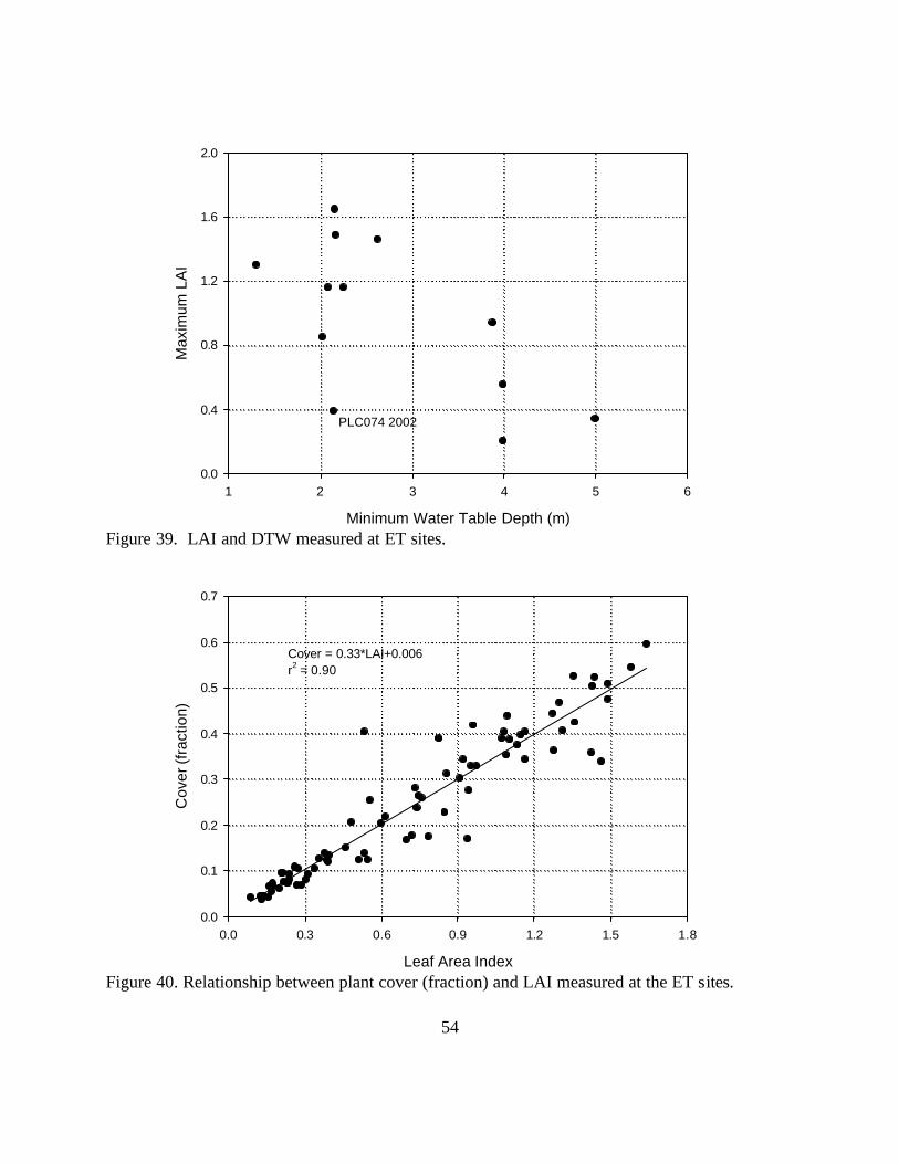
54
Minimum Water Table Depth (m)
1 2 3 4 5 6
Max
imum
LA
I
0.0
0.4
0.8
1.2
1.6
2.0
PLC074 2002
Figure 39. LAI and DTW measured at ET sites.
Leaf Area Index
0.0 0.3 0.6 0.9 1.2 1.5 1.8
Cov
er (f
ract
ion)
0.0
0.1
0.2
0.3
0.4
0.5
0.6
0.7
Cover = 0.33*LAI+0.006r2 = 0.90
Figure 40. Relationship between plant cover (fraction) and LAI measured at the ET sites.

55
approximately 10mm of rain creating a bimodal pattern in LAI and ET. This was the only site to
exhibit a noticeable response to summer precipitation. LAI was only weakly related to DTW
EC energy balance components and closure
An example of the half-hourly EB for the EC system at BLK 100 for several days in 2002
is given in Figure 41. EB ranged from (rarely) near zero to over 100 W m-2 with a mean EB
closure error over the period of 43.9 W m-2. Mean available energy during this period was 124.0
W m-2, thus the turbulent fluxes did not account for over one-third of the available energy.
During DOY 238, 2002, the energy balance closure error was greater than 150 W m-2. The
closure error tended to be highest during the afternoon, but persisted throughout the day.
Comparison of Figures 41 and 42 shows that the EB error tended to be largest during
periods of relatively higher wind speeds in the afternoon. The linear correlation coefficient
between the horizontal wind speed and the EB error was r = 0.46. Except for DOY 238, winds
were from the southeast during the afternoon, which should be the most favorable wind direction
for the EC instruments; therefore, the EB error maxima did not appear to be attributable to
disruption of the flow by the sensors and mounting structure. The peak EB closure error
occurred on DOY 238, and flow distortion may have contributed to the error that day.
For all sites, the mean EB calculated on a daily basis ranged from 47 to 94% (Figures 43
to 47). Highly erratic values of EB occurred before and after the growing season (84>DOY
>288) when all the fluxes were relatively small. Generally, the closure error was repeatable
between years at the same site and least early in the growing season and increased approximately
20% by the end of the season. The increase in closure error usually began about midsummer

56
DOY, 2002
241 242 243 244 245 246 247
Ene
rgy
bala
nce
clos
ure,
W m
-2
-50
0
50
100
150
200235 236 237 238 239 240 241
Ene
rgy
bala
nce
clos
ure,
W m
-2
-50
0
50
100
150
200
eddy covariance
Figure 41. Example of the energy balance closure error for EC system on half hourly basis at BLK 100 during the period of BR system operation.

57
DOY, 2002
241 242 243 244 245 246 247
Win
d sp
eed,
m s
-1
0
2
4
6
8235 236 237 238 239 240 241
Win
d sp
eed,
m s
-1
0
2
4
6
8
eddy covarianceBowen ratio
Figure 42. Wind speed at BLK 100 measured with eddy covariance and Bowen Ratio instruments in 2002.

58
DOY0 60 120 180 240 300 360
( λE
+ H
)/(R
n - G
)
0.0
0.2
0.4
0.6
0.8
1.0
BLK100 (2000)BLK100 (2001)
Figure 43. EB for BLK100 in 2000 and 2001.
DOY
0 60 120 180 240 300 360
( λE
+ H
)/(R n -
G)
0.2
0.4
0.6
0.8
1.0
BLK009 (2001)PLC045 (2001)
Figure 44. EB for BLK009 and BLK045 in 2001.
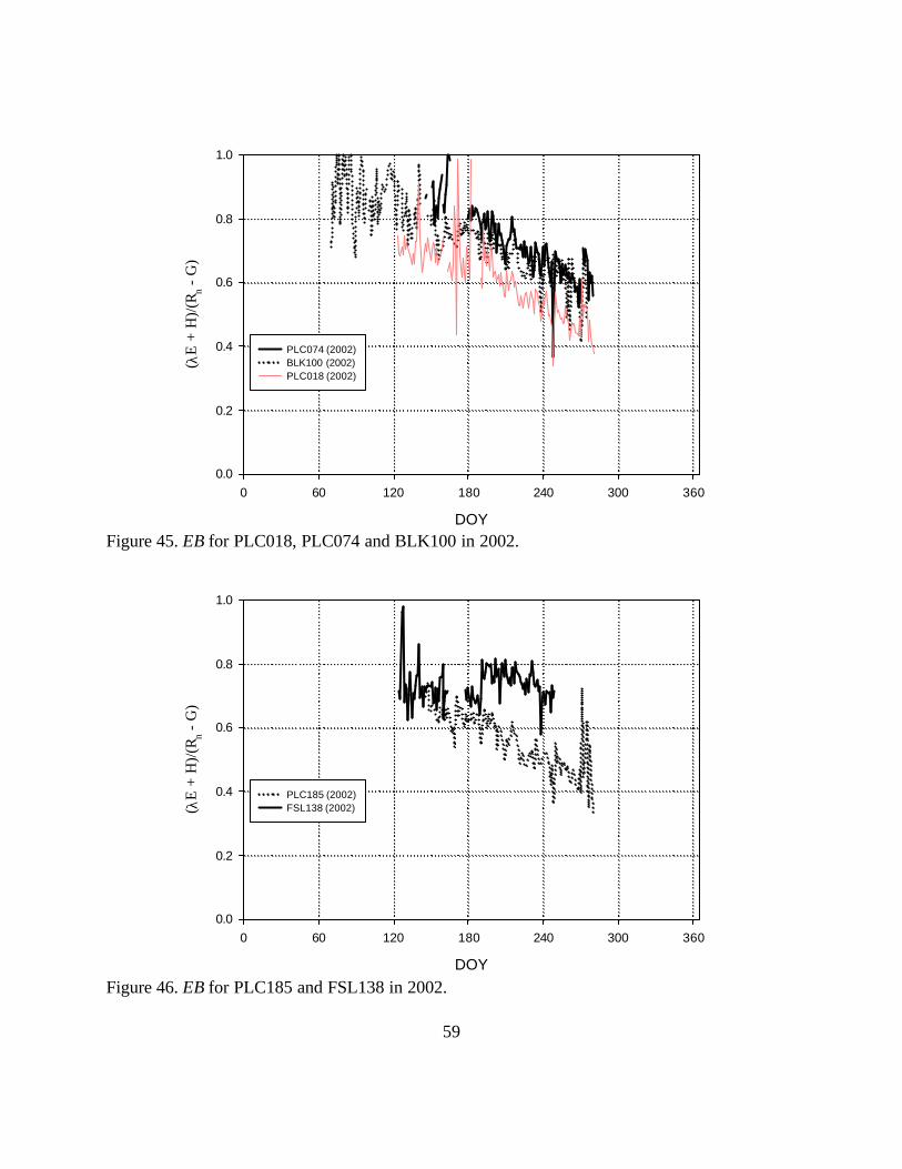
59
DOY
0 60 120 180 240 300 360
( λE
+ H
)/(R n -
G)
0.0
0.2
0.4
0.6
0.8
1.0
PLC074 (2002)BLK100 (2002)PLC018 (2002)
Figure 45. EB for PLC018, PLC074 and BLK100 in 2002.
DOY
0 60 120 180 240 300 360
( λE
+ H
)/(R n -
G)
0.0
0.2
0.4
0.6
0.8
1.0
PLC185 (2002)FSL138 (2002)
Figure 46. EB for PLC185 and FSL138 in 2002.

60
2003 Day of Year
60 120 180 240 300 360
( λE
+ H
)/(R
n - G
)
0.0
0.2
0.4
0.6
0.8
1.0
1.2
BLK100PLC074PLC185
Figure 47. EB for PLC185, PLC074 and BLK100 in 2003.
(DOY 186) and was not evident before or after the growing season. Changes in EB seem
related to H or λE individually or in combination rather than calibration drift, but the relationship
is not understood. Interestingly, the EB trend at FSL138 was not similar to trends evident at
other sites. The closure error at FSL138 was relatively stable except for a sharp decrease about
DOY 191 that corresponded with a sudden decrease in λE suggesting the closure error was
related to λE. At other sites, however, the late summer increase in the closure error was more
gradual and increased as λE decreased. The step change in closure error in BLK100 in 2003 was
an instrumentation artifact (Figure 47).
Failure of EC systems to achieve EB closure has been observed in other studies, and
various instrumental or theoretical explanations have been put forth to address the problem.

61
Zeller et al. (1989) and Massman et al. (1990) examined sources of error in EC turbulent flux
measurements due to mismatches in sensor response times, sensor volume or line averaging
effects, flow distortion around sensors and mounting structures, spatial separation of sensors, and
sampling rate (aliasing) effects. Each source of error tends to reduce the covariance measured by
the EC system, thereby causing the turbulent fluxes to be underestimated. After implementing
corrections for each of these sources of error, their energy balance still failed to achieve closure,
which they attributed to inaccuracy of the measurement of Rn and G.
In the event of non-closure of the energy balance, there are various strategies to correct
the EC fluxes. Besides the formal frequency domain transfer function corrections used by Zeller
et al. (1989) and Massman et al. (1990), several simple ad hoc corrections based on the Equation
5 can be made, the choice of which depends on the suspected source of error. If the error is due
to the hygrometer, energy balance can be achieved by assuming all the error is in the latent heat
term. If the error is due to the sonic anemometer or due to a loss of covariance that affects H and
λE in similar proportions, the turbulent fluxes can be corrected by assuming that β is measured
correctly and adjusting the magnitude of the turbulent fluxes such that energy balance is
achieved.
Examination of the EB from EC systems operated as part of this study revealed that
closure errors of similar magnitude occurred at sites with minimal ET (e.g. PLC018, Figure 45)
suggesting that both turbulent fluxes are underestimated. Also, λE measured by the EC system
at all sites was near 0 W m-2 during nighttime, as would be expected for the dry soil surface
present at the sites. Therefore, though the error may have been partly due to the hygrometer,
ascribing the EB error solely to the λE term was unwarranted. BR system β measured with the

62
DOY, 2002
241 242 243 244 245 246 247
Bow
en r
atio
0
2
4
6
8
10235 236 237 238 239 240 241
Bow
en r
atio
0
2
4
6
8
10
eddy covarianceBowen ratio
Figure 48. Daytime Bowen ratio (H/λE) at BLK 100 measured with eddy covariance and Bowen Ratio instruments in 2002. Only daytime β are shown because nighttime β for both systems tended to be highly erratic due to the small magnitude and variable sign of λE.

63
BR and EC systems agreed during daylight hours, except at times when the produced large
erratic values (Figure 48). The β values were comparable between the two systems during the
morning hours, climbing to a midday peak of ~1.7, then during the afternoon hours BR β often
grow very large while the EC β smoothly decline from their midday peak. The large afternoon β
sometimes measured by the BR system are considered erroneous, because the clear dry
conditions during the measurement period should produce smoothly varying β during daylight
hours. The cause of these erroneous measurements is unknown. During periods of afternoon
winds, the BR system often yielded unstable large Bowen ratios. Additionally, values of β
produced by the EC system followed a smoothly varying pattern repeated each day of increase
from negative values in the early morning to a midday maxima followed by decrease to negative
values in the evening. Thus, use of β measured by the EC system is probably the most reliable
way to correct the EC turbulent fluxes. The correction applied was,
1+−
=β
λGR
E ncorr (14)
Of course, when Equation 13 is used to correct the EC measurements, the computed flux is no
longer independent of the energy balance measurements. Additionally, measurements at dawn
and dusk when β is near −1 must either be discarded, similar to the processing of BR
measurements, or not be corrected. Periods when β is near −1 have little influence on daily or
seasonal ET estimates, because ET is usually low during the time of day when this condition
prevails. Prior to the application of Equation 14, the only corrections applied to the EC λE
measurement were the oxygen and air density corrections. Using β as the correction factor thus

64
DOY, 2002
241 242 243 244 245 246 247
Late
nt h
eat f
lux,
W m
-2
0
50
100
150
200
250
300235 236 237 238 239 240 241
Late
nt h
eat f
lux,
W m
-2
0
50
100
150
200
250
300
corrected eddy covarianceBowen ratio
Figure 49. Latent heat flux at BLK 100 measured with eddy covariance and Bowen Ratio instruments in 2002. EC latent heat flux has been corrected using Equation 14.

65
PLC185
Pacific standard time, July 3, 2002
Ene
rgy
flux
(W m
-2)
0
200
400
600
Net radiationSoil heat fluxLatent heatSensible heat
00:00 06:00 12:00 18:00 24:00
BLK100
Pacific standard time, July 3, 2002
Ene
rgy
flux
(W m
-2)
0
200
400
600
Net radiationSoil heat fluxLatent heatSensible heat
00:00 06:00 12:00 18:00 24:00
Figure 50. Half-hourly energy balance components measured at PLC185 (top graph) and BLK100 (bottom graph).

66
assumes that other sources of error affect the turbulent fluxes in equal proportion (i.e.,
multiplicatively). When λE measured with the EC system is corrected using Equation 14, it
produces similar results to λE measured with the BR system during periods when β produced by
both system was similar (Figure 49). During periods when β measured with the BR system was
erroneously large (e.g. at night), λEcorr was greater than that measured with the BR system.
Eddy covariance results
Two examples of the diurnal fluxes typical of summer conditions at a dry and wet site of
the Owens Valley are shown in Figure 50 where daytime surface heating due to solar radiation is
partitioned into positive daytime sensible and latent heat fluxes. Soil heat flux was a relatively
small component of the energy balance and changed sign from negative to positive in mid-
morning and from positive to negative in late evening. At night, net radiation was negative due
to thermal emission from the land surface, latent heat flux was near zero due to the cessation of
plant transpiration, and sensible heat flux was small and negative.
The λEcorr was usually, but not exclusively, greater than the uncorrected EC measurement
(Figures 51 and 52). The correction increased ET estimates a few tenths of mm day -1 up to 1
mm day-1 depending on the site. One disadvantage of adopting this correction was the shorter
record of corrected ET because there were fewer days when all instruments were functioning.
The disadvantage was particularly acute at BLK009 and PLC045 where datalogger problems
prevented collection of Rn and G for the first half of the growing season.

67
Year
Unc
orre
cted
ET
, mm
day
-1
0
1
2
3
4
5
6
BLK 100BLK 009PLC 045PLC 018FSL 138PLC 074PLC 185
2000 2001 2002
rain
rain
rain
2003
Figure 51. All uncorrected ET measured by EC systems.
Year
ET c
orr,
mm
day
-1
0
1
2
3
4
5
6
BLK 100 BLK 009PLC 045PLC 018FSL 138PLC 074PLC 185
2000 2001 2002
rain
rain
2003
Figure 52. All ET corrected for energy imbalance and fitted Fourier models used for integration.

68
Table 6. ETcorr Fourier model coefficients and r2 for each site-year. Year Site mean A(1) A(2) B(1) B(2) r2
mm day-1 2000 BLK 100 1.37 -1.62 0.26 -0.12 0.06 0.93 2001 BLK 100 1.33 -1.56 0.27 -0.13 -0.12 0.90 BLK 9 1.43 -1.65 0.31 -0.14 -0.17 0.95 PLC 45 0.50 -0.50 0.12 0.15 -0.08 0.85 2002 BLK 100 1.12 -1.33 0.30 -0.27 0.03 0.98 FSL 138 1.94 -2.28 0.50 0.10 -0.20 0.70 PLC 18 0.18 -0.14 0.01 -0.03 -0.02 0.54 PLC 74 0.60 -0.49 0.02 0.06 -0.004 0.63 PLC 185 0.35 -0.33 0.05 0.05 -0.05 0.57 2003 BLK 100 1.53 -1.92 0.33 -0.14 -0.17 0.91 PLC 74 0.81 -1.07 0.27 0.01 -0.16 0.91 PLC 185 0.68 -0.57 -0.04 0.14 -0.05 0.76
The Fourier models also are shown in Figure 52, and coefficients and fitting statistics are given
in Table 6. The relatively low r2 for PLC018 and PLC185 (Table 6) was due in large part to the
low and relatively flat seasonal ET trend (small variance). Visual inspection, however, suggests
the agreement between the data and Fourier model was acceptable for the purpose of integration..
ET at each site is described further in the next section.
Comparison of λEcorr, TKc, and TGB
Performance of the Kc and Green Book models was evaluated three ways: 1)
correspondence of TKc and TGB with trends in λEcorr, i.e. shape of the models 2) comparison of
seasonal transpiration totals estimated by TKc and TGB with λEcorr Fourier model totals, and 3)
comparison field measurements with models for individual species LAI and ETr components of
TKc and TGB (LAI only).

69
Day of Year, 2000
0 60 120 180 240 300 360
Flux
(m
m d
ay-1)
0
2
4
6ETcorr andFourier modelTKc
TGB
Figure 53. λEcorr at BLK100 in 2000 measured with the EC system and TGB and TKc estimated using measured LAI Equations 7 and 9. Fourier model fitted to λEcorr also shown.
. Day of Year, 2001
0 60 120 180 240 300 360
Flux
(m
m d
ay-1)
0
2
4
6ETcorr and Fourier modelTKc
TGB
Figure 54. λEcorr at BLK100 in 2001 measured with the EC system and TGB and TKc. Fourier model fitted to λEcorr also shown.

70
Day of Year, 2001
0 60 120 180 240 300 360
Flux
(m
m d
ay-1
)
0
2
4
6ETcorr and Fourier modelTKc TGB
ETuncorr
Figure 55. λEcorr at BLK009 in 2001 measured with the EC system and TGB and TKc. EC measurements corrected and uncorrected for energy balance closure error are presented. Fourier model fitted to λEcorr also shown.
Day of Year, 2001
0 60 120 180 240 300 360
Flux
(m
m d
ay-1
)
0
2
4
6
ETcorr andFourier modelTKc
TGB
ETuncorr
Figure 56. λEcorr at PLC045 in 2001 measured with the EC system and TGB and TKc. EC measurements corrected and uncorrected for energy balance closure error are presented. Fourier model fitted to λEcorr also shown.

71
Day of Year, 2002
0 60 120 180 240 300 360
Flu
x (m
m d
ay-1 )
0
2
4
6ETcorr andFourier modelTKc
TGB
Figure 57. λEcorr at BLK100 in 2002 measured with the EC system and TGB and TKc. Fourier model fitted to λEcorr also shown.
Day of Year, 2002
0 60 120 180 240 300 360
Flux
(m
m d
ay-1)
0
2
4
6ETcorr andFourier modelTKc
TGB
Figure 58. λEcorr at FSL138 in 2002 measured with the EC system and TGB and TKc. Fourier model fitted to λEcorr also shown.

72
Day of Year, 2002
0 60 120 180 240 300 360
Flux
(m
m d
ay-1)
0
2
4
6ETcorr andFourier model TKc
TGB
rain
Figure 59. λEcorr at PLC018 in 2002 measured with the EC system and TGB and TKc. Fourier model fitted to λEcorr also shown.
Day of Year, 2002
0 60 120 180 240 300 360
Flux
(m
m d
ay-1)
0
2
4
6ETcorr andFourier modelTKc
TGB
rain
Figure 60. λEcorr at PLC074 in 2002 measured with the EC system and TGB and TKc. Fourier model fitted to λEcorr also shown.

73
Day of Year 2002
0 60 120 180 240 300 360
Flux
(m
m d
ay-1)
0
2
4
6ETcorr andFourier modelTKc
TGB
Figure 61. λEcorr at PLC185 in 2002 measured with the EC system and TGB and TKc. Fourier model fitted to λEcorr also shown.
Day of Year, 2003
0 60 120 180 240 300 360
Flux
(m
m d
ay-1)
0
1
2
3
4
5
6
ETcorr and
Fourier modelTGB
TKc
Figure 62. λEcorr at BLK100 in 2003 measured with the EC system and TGB and TKc. Fourier model fitted to λEcorr also shown.

74
Day of Year, 2003
0 60 120 180 240 300 360
Flux
(m
m d
ay-1)
0
1
2
3
4
5
6
ETcorr andFourier modelTKc
TGB
Figure 63. λEcorr at PLC074 in 2003 measured with the EC system and TGB and TKc. Fourier model fitted to λEcorr also shown.
Day of Year, 2003
0 60 120 180 240 300 360
Flux
(m
m d
ay-1)
0
1
2
3
4
ETcorr andFourier modelTGB
TKc
Figure 64. λEcorr at PLC185 in 2003 measured with the EC system and TGB and TKc. Fourier model fitted to λEcorr also shown.

75
Seasonal trends in ET corresponded with the expected trends in evaporative demand throughout
the summer. ET peaked in midsummer and was greater at sites with higher LAI. Daily values of
λEcorr and fitted Fourier models are presented in Figures 53 to 64 along with TKc and TGB. At
grass-dominated sites, TGB exceeded TKc, but relative magnitudes were reversed at shrub-
dominated sites consistent with the comparison by Steinwand (2000b). At most sites, TKc and
TGB usually underestimated early and late season λEcorr, but overestimated midsummer λEcorr.
Seasonal TKc and TGB loosely tracked λEcorr at BLK100 (all years), PLC074, and PLC185 (2002).
Seasonal trends in TKc and TGB compared less favorably with field measurements at BLK009,
FSL138, PLC045, and PLC018. At PLC045, and PLC018, the poor agreement was likely due to
failure of site conditions to meet model assumptions. At PLC045 and PLC018, the water table
was at or below the maximum rooting depth for saltbush and rabbitbrush, respectively, and the
upper 4 to 5 meters of soil was near the limiting water content. Both models assume soil water is
sufficient, and therefore, it was not surprising that TKc and TGB overestimated the observed ET.
The decline in LAI and ET (inferred from decline in uncorrected λE) during June at PLC045
corresponded with the exhaustion of available soil water within the monitored soil depth ( 3.3m)
by June 21 (Figure 56) suggesting that the uptake rate of groundwater alone was insufficient to
support early season leaf area. Subsequently, leaf area and ET at this site responded to
approximately 35 mm of rain in early July (Figure 38). The TKc and TGB models cannot
accommodate the bimodal response exhibited at this site, and the seasonal ET total based on the
Fourier model integration is overestimated. At FSL138, TGB tracked λEcorr better than TKc, but
neither model estimated the seasonal total well or tracked the early (April and May) and late
(August and Sept.) season ET. The sharp decline in λEcorr at FSL138 on July 11 corresponded

76
Table 7. RMSE between eddy covariance ET corrected for energy balance closure and T estimated from Kc and GB models.
Year Site TKc RMSE ^ June Meas.
TKc RMSE July Meas.
TGB RMSE June Meas.
TGB RMSE July Meas.
mm day-1 2000 BLK 100 0.58 0.71 0.98 1.13 2001 BLK 100 0.71 0.72 1.02 0.94 BLK 9 0.85 0.74 0.97 1.00 PLC 45 0.49 0.49 0.52 0.26 2002 BLK 100 0.61 0.51 0.75 0.92 FSL 138 2.10 1.48 1.65 1.16 PLC 18 0.60 0.25 0.56 0.25 PLC 74 0.40 0.42 0.49 0.54 PLC 185 0.19 0.23 0.24 0.29 2003 BLK 100 0.95 0.98 0.94 0.97 PLC 74 0.48 0.50 0.63 0.86 PLC 185 0.48 0.52 0.63 0.65
^: RMSE = [3(ETcorr-model)2/n]0.5
with termination of soil water uptake at depths above 1 m and with the deepest water table depth
(2.05 m). This site had the shallowest water table of all sites, and the λEcorr decline may reflect a
decrease in surface E as the soil dried and/or decrease in T as the water table approached the
bottom of the saltgrass root zone of approximately 2 m (Groeneveld, 1990). Total LAI began to
decline steadily after the July 9 measurement suggesting that curtailed transpiration constituted
some fraction of the observed reduction in λEcorr. Most of the change in LAI was due to decline
in DISP2. Vegetation at this site also had a significant component of beardless wildrye, Leymus
triticoides and minor amounts of Juncus sp. The LAI of species without known Kc was
approximately 40% of the total LAI at the peak of the summer. It is not known if differing
physiology of these species contributed to the observed ET step change. Failure of the models at
BLK009 was not easily attributable to substantial E or plant water stress, and the large difference
from measured ET may reflect an inherent inability of both

77
Table 8. Eddy covariance ET corrected for energy balance closure and T model predictions. LAI data collected in early June and July (before and after the solstice) were used to bracket the Kc and GB model predictions of T. TKc relied on mean daily ETr. Measured and predicted fluxes are the sum of daily totals extrapolated for the growing season (March 25 to October 15).
Year Site ETcorr TKc June TKc July TGB June TGB July mm 2000 BLK 100 460 450^ 478 479 521 2001 BLK 100 446 399 369 450 415 BLK 9 471 652 569 487 405 PLC 45 165^^ 254 245 166 90 2002 BLK 100 377 273 340 311 376 FSL 138 646 284 388 347 484 PLC 18 53 195 100 116 60 PLC 74 177 133 120 94 80 PLC 185 108 77 62 59 46 2003 BLK 100 527 330 314 367 346 PLC 74 282 292 207 193 135 PLC 185 205 112 97 60 56
^: Shaded values represent measurement date nearest the solstice (TGB) or the maximum LAI in the TKc model for the dominant species. ^^: This value is exaggerated because of the poor correspondence of the shape of the Fourier model with the bimodal ET trend.
models for the dominant species, CHNA2. Although there were no obvious signs of water
deficit in the LAI or appearance of the grasses, overestimation of the grass ET component cannot
be ruled out with certainty because the water table was near the typical maximum rooting depth
for SPAI, the second most abundant species at the site.
The model agreement with daily λEcorr was evaluated by calculating the root mean
squared error (RMSE) between TKc or TGB and measured daily λEcorr. Usually, RMSE of TKc was
smaller than the corresponding TGB (Table 7) suggesting the former model better approximates
the overall progression of ET through the season. Performance for both models was poorest at
FSL138, but the low RMSE for BLK009 and PLC045 were deceptive because the period with
available λEcorr was limited to late July and after. Large suspected differences between the

78
Measured ETcorr (mm)
0 100 200 300 400 500 600 700
Pre
dict
ed tr
ansp
iratio
n (m
m)
0
100
200
300
400
500
600
700
1:1 lineTKc
TGB
Figure 65. Predicted growing season transpiration from the Kc and GB models (shaded cells in Table 8) plotted against measured ET. PLC045 and PLC018 not plotted.
models and ET earlier in the growing season when λEcorr could not be calculated (Figures 55 and
56) and were not included in the RMSE calculation.
ETcorr summed for the growing season the growing season ranged between 53 and 646
mm (Table 8). Measured ET agreed best with TKc predictions of transpiration for five site-years:
BLK100, 2002; PLC074, 2002; PLC074, 2003; PLC185, 2002; and PLC185, 2003. TGB
performed better for four site-years: BLK100, 2001; BLK100, 2003; BLK009; and FSL138. The
model estimated totals were essentially equal for one site-year, BLK100 in 2000. Comparisons
for PLC018 and PLC045 were not informative because conditions at those sites clearly violated
assumptions of sufficient soil water present in both models. Better agreement with the seasonal
totals at these sites should be considered a failure in the models. Mean difference between

79
predicted and measured ET (n=10) was virtually identical; 88mm for TKc and 90mm for TGB.
Considering forecasted water requirements at monitoring sites using the Green Book method
typically are less than 300 to 400mm, an average error of this magnitude is of considerable
concern. TKc and TGB varied several centimeters depending on which LAI measurements
bracketing the midsummer solstice were used. In four instances the difference between seasonal
totals using June and July LAI measurements in the same model was larger than the difference
between the TKc and TGB models. In those cases, reliance on a single midsummer measurement
date determined a priori to represent the maximum LAI was as large a source of error as model
selection. Based on a simple tabulation of the sites, the Kc performed marginally better (five to
four) but given the relatively large error and variation caused by matching measured and
modeled peak LAI, the appropriate conclusion is that the models performed equally.
Overall, both models usually underestimated measured ET (Figure 65). Underestimation
by the transpiration models could have been caused by bare soil E and direct evaporation of
precipitation sensed by the EC instruments but not accounted for by the transpiration models.
Summer precipitation was small, less than 15 mm except for PLC045 (35mm), BLK100 in 2003
(38mm), and PLC185 in 2003 (17mm), so the impact of direct evaporation on measured ET was
negligible. The primary method to minimize bare soil evaporation in this study was to avoid
sites with water tables near the surface. Bare soil evaporation is a two stage process.
Evaporation of the first stage with wet soil at the surface is limited by available energy; second
stage evaporation is limited by the rate of unsaturated water transport through a dry surface layer.
The surface layers (0-12 cm or deeper) were near the limiting water content for most of the
growing season suggesting the flux through the bare surface was small (Hillel, 1980), yet the

80
contribution of evaporation from winter precipitation held in the shallow soil layers early in the
growing season cannot be easily discounted. Jacobs et al. (2002) found that the transition to
second stage evaporation in Florida wetlands was marked by an increase in sensible heat and
decrease in latent heat flux. No such transition was evident in this study except at PLC045 from
DOY 130 to DOY 183. Also, the models often overestimated midsummer ET and
underestimated late summer ET, long after winter precipitation was exhausted. Underestimation
by the transpiration models in this study was apparently the due to a deficiency in the shape of
the models and not failure to account for a significant flux measured by the EC towers.
The GB and Kc models contain submodels for LAI and mean ETri (Kc only), that can be
compared with field measurements to lend insight into factors affecting the overall model
performance. As before, LAI measured nearest the summer solstice was used in the GB model,
and LAI measured nearest the date of maximum LAI for the dominant species was used in the
Kc model (Table 4). The GB LAI models underestimated LAI for nearly all species and sites
except possibly for SAVE at PLC074 (Figures 65 to 79). The Kc LAI models nearly always
modeled LAI better than the GB models but still underestimated LAI for species at BLK100,
BLK009 and PLC018. Performance of both models could have been improved by choosing an
alternate measurement date(s) instead of relying on a fixed LAI measurement date to fix the
maximum LAI in the model. The maximum LAI for individual species was often a month or
more shifted from the Kc and GB model peak LAI. The agreement between the timing of
observed and modeled peak LAI, however, was slightly better for the Kc model.
Mean daily ETr tracked measured ETr well except for short periods in midsummer all
four years (Figure 80). The disagreement was most evident in June and July, 2001 and 2002 and

81
Day of Year, 2000
0 60 120 180 240 300 360
LAI
0.0
0.2
0.4
0.6
0.8
1.0
DISP2 LAIKc DISP2 model GB DISP2 model
Day of Year, 2000
0 60 120 180 240 300 360
LAI
0.0
0.2
0.4
0.6
0.8
1.0
SPAI LAIKc SPAI model GB SPAI model
Figure 66. Measured LAI for dominant species, SPAI and DISP2, at BLK100 in 2000 and LAI models in TKc (Steinwand, 1998) and TGB. Measured LAI is the mean of the four transects. Measurements taken on July 7 were used to set the maximum of the LAI models.

82
Day of Year, 2001
0 60 120 180 240 300 360
LAI
0.0
0.2
0.4
0.6
0.8
1.0
DISP2 LAIKc DISP2 model GB DISP2 model
Day of Year, 2001
0 60 120 180 240 300 360
LAI
0.0
0.2
0.4
0.6
0.8
1.0
SPAI LAIKc SPAI model GB SPAI model
Figure 67. Measured LAI for dominant species, SPAI and DISP2, at BLK100 in 2001 and LAI models in TKc (Steinwand, 1998) and TGB. Measured LAI is the mean of the four transects. Measurements taken on July 9 were used to set the maximum of the LAI models.

83
Day of Year, 2001
0 60 120 180 240 300 360
LAI
0.0
0.2
0.4
0.6
0.8
1.0
SPAI LAIKc SPAI model GB SPAI model
Day of Year, 2001
0 60 120 180 240 300 360
LAI
0.0
0.2
0.4
0.6
0.8
1.0
CHNA2 LAIKc CHNA2 model GB CHNA2 model
Figure 68. Measured LAI for dominant species, SPAI and CHNA2, at BLK009 in 2001 and LAI models in TKc (Steinwand, 1998) and TGB. Measured LAI is the mean of the four transects. Measurements taken on July 11 were used to set the maximum of the LAI models.

84
Day of Year, 2001
0 60 120 180 240 300 360
LAI
0.0
0.2
0.4
0.6
0.8
1.0
ATTO LAIKc ATTO model GB ATTO model
Figure 69. Measured LAI for dominant species, ATTO, at PLC045 in 2001 and LAI models in TKc (Steinwand, 1998) and TGB. Measured LAI is the mean of the four transects. Measurements taken on July 9 were used to set the maximum of the LAI models. Neither model was designed to accommodate the bimodal pattern exhibited at this site.

85
Day of Year, 2002
0 60 120 180 240 300 360
LAI
0.0
0.2
0.4
0.6
0.8
1.0
DISP2 LAIKc DISP2 model GB DISP2 model
Day of Year, 2002
0 60 120 180 240 300 360
LAI
0.0
0.2
0.4
0.6
0.8
1.0
SPAI LAIKc SPAI model GB SPAI model
Figure 70. Measured LAI for dominant species, SPAI and DISP2, at BLK100 in 2002 and LAI models in TKc (Steinwand, 1998) and TGB. Measured LAI is the mean of the four transects. Measurements taken on July 10 were used to set the maximum of the LAI models.

86
Day of Year, 2002
0 60 120 180 240 300 360
LAI
0.0
0.2
0.4
0.6
0.8
1.0
ATTO LAI Kc ATTO model GB ATTO model
Day of Year, 2002
0 60 120 180 240 300 360
LAI
0.0
0.2
0.4
0.6
0.8
1.0
DISP2 LAIKc DISP2 model GB DISP2 model
Figure 71 Measured LAI for dominant species, ATTO and DISP2, at PLC074 in 2002 and LAI model in TKc (Steinwand, 1998) and TGB. Measured LAI is the mean of the four transects. Measurements taken on June 5 were used to set the maximum of the LAI models.
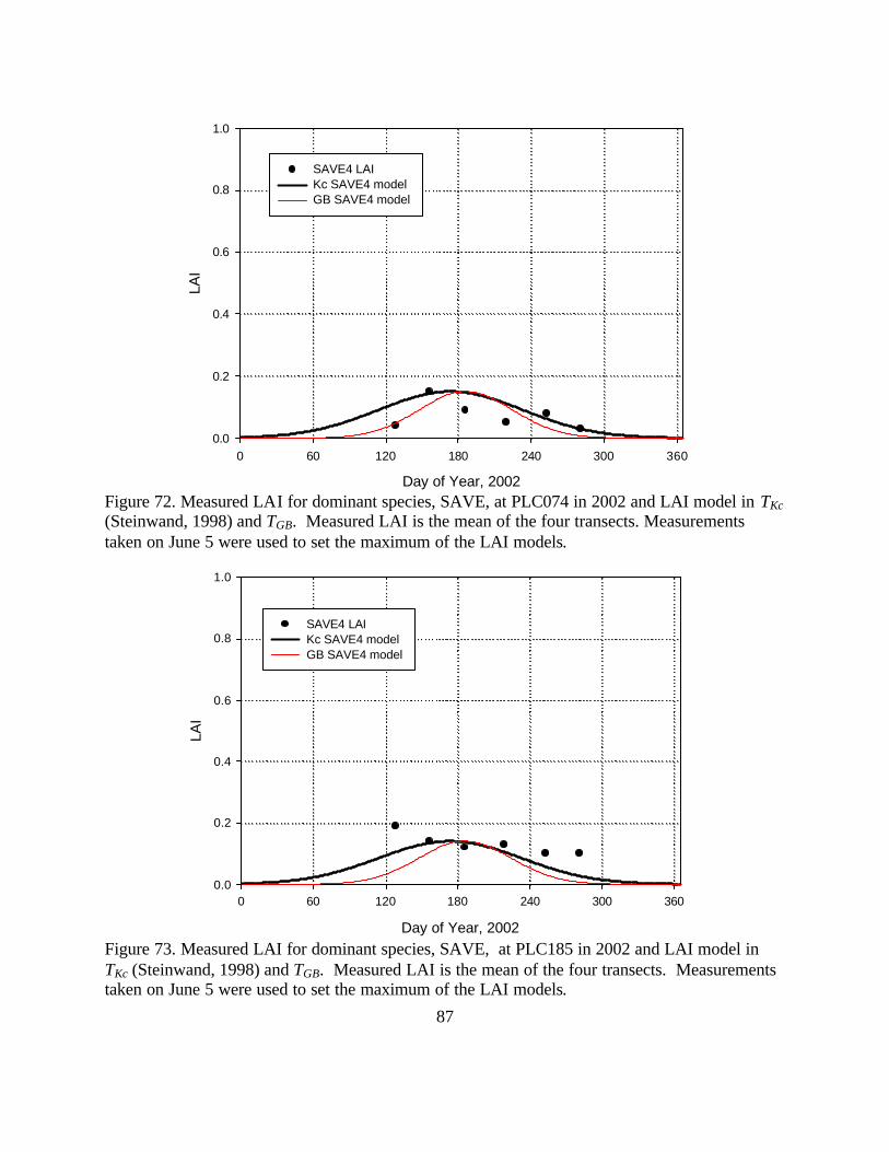
87
Day of Year, 2002
0 60 120 180 240 300 360
LAI
0.0
0.2
0.4
0.6
0.8
1.0
SAVE4 LAI Kc SAVE4 model GB SAVE4 model
Figure 72. Measured LAI for dominant species, SAVE, at PLC074 in 2002 and LAI model in TKc (Steinwand, 1998) and TGB. Measured LAI is the mean of the four transects. Measurements taken on June 5 were used to set the maximum of the LAI models.
Day of Year, 2002
0 60 120 180 240 300 360
LAI
0.0
0.2
0.4
0.6
0.8
1.0
SAVE4 LAI Kc SAVE4 model GB SAVE4 model
Figure 73. Measured LAI for dominant species, SAVE, at PLC185 in 2002 and LAI model in TKc (Steinwand, 1998) and TGB. Measured LAI is the mean of the four transects. Measurements taken on June 5 were used to set the maximum of the LAI models.

88
Day of Year, 2002
0 60 120 180 240 300 360
LAI
0.0
0.2
0.4
0.6
0.8
1.0
DISP2 LAIKc DISP2 model GB DISP2 model
Figure 74. Measured LAI for dominant species, DISP2, at FSL138 in 2002 and LAI model in TKc (Steinwand, 1998) and TGB. Measured LAI is the mean of the four transects. Measurements taken on July 8 were used to set the maximum of the LAI models.
Day of Year, 2002
0 60 120 180 240 300 360
LAI
0.0
0.2
0.4
0.6
0.8
1.0
CHNA2 LAIKc CHNA2 model GB CHNA2 model
Figure 75. Measured LAI for dominant species, CHNA2, at PLC018 in 2002 and LAI model in TKc (Steinwand, 1998) and TGB. Measured LAI is the mean of the four transects. Measurements taken on July 8 were used to set the maximum of the LAI models

89
Day of Year, 2003
0 60 120 180 240 300 360
LAI
0.0
0.2
0.4
0.6
0.8
1.0
DISP2 LAIKc DISP2 modelGB DISP2 model
Day of Year, 2003
0 60 120 180 240 300 360
LAI
0.0
0.2
0.4
0.6
0.8
1.0
SPAI LAIKc SPAI modelGB SPAI model
Figure 76. Measured LAI for dominant species, SPAI and DISP2, at BLK100 in 2003 and LAI models in TKc (Steinwand, 1998) and TGB. Measured LAI is the mean of the four transects. Measurements taken on July 14 were used to set the maximum of the LAI models.

90
Day of Year, 2003
0 60 120 180 240 300 360
LAI
0.0
0.2
0.4
0.6
0.8
1.0
ATTO LAIKc ATTO model GB ATTO model
Day of Year, 2003
0 60 120 180 240 300 360
LAI
0.0
0.2
0.4
0.6
0.8
1.0
DISP LAIKc DISP model GB DISP model
Figure 77. Measured LAI for dominant species, ATTO and DISP2, at PLC074 in 2003 and LAI model in TKc (Steinwand, 1998) and TGB. Measured LAI is the mean of the four transects. Measurements taken on June 9 were used to set the maximum of the Kc LAI models and July 15 for GB models

91
Day of Year, 2003
0 60 120 180 240 300 360
LAI
0.0
0.2
0.4
0.6
0.8
1.0
SAVE4 LAI Kc SAVE4 model GB SAVE4 model
PLC074
Figure 78. Measured LAI for dominant species, SAVE, at PLC074 in 2003 and LAI model in TKc (Steinwand, 1998) and TGB. Measured LAI is the mean of the four transects. Measurements taken on June 9 were used to set the maximum of the Kc LAI models and July 15 for GB models
Day of Year, 2003
0 60 120 180 240 300 360
LAI
0.0
0.2
0.4
0.6
0.8
1.0
SAVE4 LAI Kc SAVE model GB SAVE4 model
PLC185
Figure 79. Measured LAI for dominant species, SAVE, at PLC185 in 2003 and LAI model in TKc (Steinwand, 1998) and TGB. Measured LAI is the mean of the four transects. Measurements taken on June 10 were used to set the maximum of the Kc LAI models and July 15 for GB models

92
Date
1/1/2000 7/1/2000 1/1/2001 7/1/2001 1/1/2002 7/1/2002 1/1/2003 7/1/2003 1/1/2004
ET
r (m
m d
ay-1
)
0
1
2
3
4
5
6
7
8
9
10
ET r mean daily ETr
Figure 80. Mean daily ETr and daily ETr measured in 2000-2002 at the CIMIS station in Bishop, Ca.
was probably due to hotter than average temperatures. If the actual daily ET values were utilized
instead of the modeled daily mean, TKc estimates increase slightly for 2001-2002, decrease
slightly for 2000, and are essentially unchanged in 2003. The inclusion of ETr in the Kc model
probably wasn’t a large source of the deviation from ETcorr.
Conclusions and Recommendations
Eddy covariance measurements of ET were collected successfully during most of the
growing season at seven sites over four years. Turbulent fluxes measured by the EC system,

93
however, did not account for approximately one-third of the available energy, similar to
discrepancies observed in other studies using EC methods. A comparison with a Bowen ratio
station at one site was conducted to examine the energy imbalance further. During periods when
the BR system obtained stable measurements, the Bowen ratios measured by the two systems
substantially agreed, allowing use of the Bowen ratio measured by the EC system to correct λE
and H to account for all the available energy.
The comparison of growing season ET measured by the EC systems and model
predictions based on vegetation measurements did not show conclusively which model should be
favored for groundwater management. Both models generally tracked the progression of ET
through the growing season although the consistent underestimation early and late in the growing
season suggest an inherent deficiency in the shape of the models. Usually the difference
between the modeled and measured values of daily ET was smaller for the Kc model than the
GB model. Likewise, the LAI models used to prepare the original Kc clearly agreed better with
measured values for dominant species than the GB LAI model although performance of both sets
of models often was limited by the procedure to fix maximum LAI for all species by a single
midsummer measurement. Both models provide “ballpark” estimates that roughly correspond
with independent ET measurements suggesting the assumptions necessary to scale up models
derived from porometric data were largely met. Both the Kc and GB models, however, tended to
underestimate total growing season ET, and transpiration estimates for the growing season best
agreed with measured ET for essentially equal numbers of site-years with the TKc model
performing marginally better. Poor predictions of actual ET occurred despite the attempt to
select sites to conform with the model assumptions.

94
From this study, it is not obvious that either model should be favored for groundwater
pumping management although the performance of the Kc models and its LAI component was
marginally superior. Additional advantages of the Kc models described in previous Inyo County
reports include better documentation of methods and data upon which they are based and the
capability to subject the model prediction to error analysis. The relatively large average error,
occasional poor performance, and frequent underestimation of actual ET suggest either model
must be used with due regard for its imprecision. Ignoring prediction error in these models for
pumping management is not advised.
Presentations
Steinwand, A.L., R.F. Harrington, P.J. Hubbard, and D. Martin. 2002. Transpiration coefficients and eddy covariance estimates of evapotranspiration of Great Basin phreatophytes. In Agronomy Abstracts, ASA, Madison, WI. Steinwand, A.L., R.F. Harrington, and D. Or. 2003. Water balance closure for Owens Valley phreatophytes combining water table, eddy covariance, and soil water measurements. In Agronomy Abstracts, ASA, Madison, WI.
References
Allen, R.B., L.S. Pereira, D. Raes, and M.S. Smith. 1998. Crop ET, Irrigation, and Drainage. Paper #56. Food and Agriculture Organization of the United Nations. Rome, Italy.
Arya, S.P. 2001. Introduction to Micrometeorology, Second Edition, Academic Press. Berger, D.L., M.J. Johnson, and M.L. Tumbusch. 2001. Estimates of Evapotranspiration from
the Ruby Lake National Wildlife Refuge Area, Ruby Valley, Northeastern Nevada, May 1999-October 2000. USGS Water Resources Investigations Report 01-4234.
Bidlake, W.R. 2000. Evapotranspiration from a Bulrush-Dominated Wetland in the Klamath
Basin, Oregon. J. of Amer. Water Res. Assoc. 36(6), 1309-1320.

95
Bidlake, W.R. 2002. Evapotranspiration from Selected Fallowed Fields on the Tule Lake National Wildlife Refuge, California, During May to October 2000, USGS Water Resources Investigations Report 02-4055.
Blake, G.R., and K.H. Hartage. 1986. Bulk density. In A. Klute (ed.) Methods of soil analysis.
Part 1. 2nd ed. Agronomy 9:363-376. Brutsaert, W. 1982. Evaporation into the atmosphere. D. Reidel. Campbell Scientific Inc. 1998a. CSAT Three Dimensional Sonic Anemometer Instruction
Manual, Revision 3/98. Campbell Scientific Inc. 1998b. Eddy Covariance System Operator's Manual CA27 and KH20,
Revision 7/98. Campbell Scientific Inc. 1989. KH20 Krypton Hygrometer, Revision 11/89. Campbell Scientific Inc. 1996. Q-7.1 Net Radiometer, Revision 5/96. Campbell Scientific Inc. 1996. CS615 Water Content Reflectometer Instruction Manual, Version
8221-07, Revision 10/96. Campbell Scientific Inc. 1999. HFT3 Soil Heat Flux Plate, Revision 2/99. Campbell, G.S., and J.M. Norman. 1998. An Introduction to Environmental Biophysics, Second
Edition, Springer. CIMIS, California Irrigation Management Information System. 2003. Agric. Water Conservation
Section, Dept. of Water Resources, Sacramento, CA. Duell, L.F.W. 1990. Estimates of Evapotranspiration in Alkaline Scrub and Meadow
Communities of Owens Valley, California, Using the Bowen-Ratio, Eddy-Correlation, and Penman-Combination Methods. USGS Water Supply Paper 2370-E.
Gash, J.H.C. 1986. A not on estimating the effect of a limited fetch on micrometeorological
evaporation measurements. Bound.-Layer Met. 35:409-413. Graupe, D. and D.I. Krause, 1973. On the identification of input-output noise models. Int. J.
Syst. Sci. 4:617-621. Groeneveld, DP. 1990. Deep root trench study. Report to Inyo/LA Technical Group. December
17, 1990. 44pp. Hillel, D. 1980. Introduction to soil physics. Academic Press, Inc., London, U.K.

96
Jacobs, J.M., S.L. Mergelsberg, A.F. Lopera, D.A. Myers. 2002. Evapotranspiration from a wet
prairie wetland under drought conditions: Paynes Prairie Preserve, Florida, USA. Wetlands. 22:374-385.
Manning, S.J., J.F. Mustard, and A.J. Elmore. 1999. Patterns of vegetation response to
groundwater pumping detected with field monitoring and LandSat TM data. Ecological Society of America. August 1999. Spokane, WA. Ecological Society of America abstracts vol. 84.
Massman, W.J., D.G. Fox, K.F. Zeller, and D. Lukens. 1990.Verifying Eddy Correlation
Measurements of Dry Deposition: A Study of the Energy Balance Components of the Pawnee Grasslands. USDA Rocky Mountain Forest and Range Experiment Station Research Paper RM-288.
Norman J.M. and J.L. Baker. 2002. Have eddy-flux measurements improved over thirty years.
Agronomy Abstracts, American Society of Agronomy, Madison, WI. Or, D., and D.P. Groeneveld. 1994. Stochastic estimation of plant-available soil water under
fluctuating water table depths. J. Hydrol. 163:43-64. Salas, J.D., W. Delleur, V. Yevjevich, and W.L. Lane. 1980. Applied modeling of hydrologic
time series. Water Resource Publications, Fort Collins, Co. Shuttleworth, W. J. 1993. Evaporation. In Handbook of Hydrology, ed. D. R. Maidment,
McGraw-Hill. Steinwand, A.L. 1998. Evaluation of methods to calculate vegetation water requirements for the
Owens Valley, Ca. Report to the Inyo/Los Angeles Technical Group, February 28, 1998. 55pp.
Steinwand, A.L, 1999a. Transpiration coefficients for three Great Basin shrubs. Report to the
Inyo/Los Angeles Technical Group, May 12, 1999. 41pp. Steinwand, A.L. 1999b. Transpiration coefficients for two Great Basin phreatophytic grasses.
Report to the Inyo/Los Angeles Technical Group, November 24, 1999. 91pp. Steinwand, A.L. 2000a. Comparison of Green Book and Kc calculations to estimate vegetation
water requirements. Report to the Inyo/Los Angeles Technical Group, February 3, 2000. 14 pp.
Steinwand, A.L. 2000b. The Effects of Kc and Green Book models for vegetation water
requirements on permanent monitoring site On/Off status. Report to the Inyo/Los Angeles Technical Group, April 24, 2000. 47pp.

97
Steinwand, A.L., R.F. Harrington, and D.P. Groeneveld. 2001. Transpiration coefficients for
three Great Basin shrubs. J. Arid Env. 49:555-567. Steinwand, A.L, and R.F. Harrington. 2003. Water table fluctuations resulting from management
under the Drought Recovery Policy and the Green Book, 1989 to 2000. Report to the Inyo/Los Angeles Technical Group, February 25, 2003. 44pp.
Steinwand, A.L. and D. Olsen. 2003. Calibration and operation of Hydrosense™ TDR for
measuring soil water at shallow depths. Report to the Inyo/Los Angeles Technical Group, December 9, 2003. 10pp.
Sumner, D.M. 1996. Evapotranspiration from Successional Vegetation in a Deforested Area of
the Lake Wales Ridge, Florida. USGS Water Resources Investigations Report 96-4244. Webb, E. K., G. I. Pearman, and R. Leuning. 1980. Correction of flux measurements for density
effects due to heat and water vapor transfer. Quart. J. R. Meteorol. Soc., 106, 85-100. Zeller, K.F., W. Massman, D. Stocker, D.G. Fox, D. Stedman, and D. Hazlett. 1989. Initial
Results from the Pawnee Eddy Correlation System for Dry Acid Deposition Research. USDA Rocky Mountain Forest and Range Experiment Station Research Paper RM-282.

98
Appendix A: Daily eddy covariance, energy balance component, and transpiration model results.
Note that some obviously erroneous data have not been culled, and the data have not be rounded
to significant figures to prevent rounding errors in the future if results presented in this
Appendix are utilized for another purpose.