Ethnic Favoritism

Robin Burgess∗ Remi Jedwab†

Edward Miguel‡ Ameet Morjaria§ Gerard Padro i Miquel¶

August 2011‖

-PRELIMINARY DRAFT-

Abstract

A large literature emphasizes the existence of ethnic favoritism. Yet, there are fewquantitative studies that extend beyond using the ethno-linguistic fractionalizationindex. This paper documents systematically the magnitude of ethnic favoritism. Inparticular, we investigate road building in Kenya by putting together novel datasets:a panel dataset on road development for the entire history of modern Kenya andsplicing this with historical data on the ethnicity of political leaders. We set up asimple framework which uses two plausibly exogenous variations in political changesto see the effects on ethnic favoritism. These changes are: (i) changes in the identityof the leader, and (ii) regime changes within the same leader to test whether co-ethnics of leaders receive more roads. We find robust evidence that political regimechanges matter. Under autocracy, leaders disproportionately invest in those districtswhere their ethnicity is dominant, however this effect is attenuated when the sameleaders are in a democratic setting, in favor of other tribes. The results suggest thatthe effect of democracy is to increase constraints on the leader.

Keywords: Democracy, Public Goods, Ethnic Politics, AfricaJEL classification codes: H41, H54, O12, O55, P16

∗London School of Economics; r.burgess@lse.ac.uk†Paris School of Economics; jedwab@pse.ens.fr‡University of California, Berkeley; emiguel@econ.berkeley.edu§Harvard Academy; ameet morjaria@harvard.edu¶London School of Economics; g.padro@lse.ac.uk‖We would like to thank Tim Besley, Oriana Bandiera, Greg Fisher, James Habyarimana, Asim

Khwaja, Guy Michaels, Jim Snyder, Jim Robinson, Eliana La Ferrara, Jean-Philippe Platteau, DenisCogneau, Konrad Burchardi, Gani Aldashev and seminar audiences at LSE-EOPP, PSE, World BankConference on Infrastructure & Development (Toulouse), NEUDC-2010 (MIT), UK-Public Economics2010 (Warwick), CEPR Development Economics Symposium (Stockholm), Harvard Development Lunchand Namur University for very helpful comments. This research is an output from funding by the UKDepartment for International Development (DFID) as part of the iiG, a research programme to studyhow to improve institutions for pro-poor growth in Africa and South-Asia. The views expressed are notnecessarily those of DFID.

1 Introduction

Scholarly work in economics and political science has emphasized the existence and

widespread prevalence of ethnic favoritism, yet the primary focus has been on looking

at the effects of ethno-linguistic fractionalization (ELF) on outcomes (e.g. growth, pro-

vision of public goods etc.) The literature seems to have stepped aside from quantifying

the extent and magnitude as well the mechanisms at play behind ethnic favoritism.1 This

could be partially explained by the difficulty of measuring ethnic favoritism as govern-

ments are often reluctant to publish disaggregated budgetary data that indicates their

geographical location. In this paper, we are able to overcome this serious challenge by

tracking road development (both expenditure budgets and physical building) in Kenya.

Kenya provides an ideal laboratory for testing as well as understanding the mecha-

nisms behind ethnic favoritism. Firstly, ethnicity is salient in the Kenyan political space,

with a large collection of anecdotal evidence on ethnic patronage (Posner 2005; Wrong

2009; Morjaria 2011; Kramon and Posner 2011a). Secondly, administratively the coun-

try is governed at the district level and ethnic groups are homogenous within a district.

Thirdly, we are able to track road development at the district level by using development

budgets and mapping them onto a GIS database. Fourthly, even though our focus is on

one country, the evolution of Kenya in terms of both political regime and growth can be

seen as a basket case in the context of Sub-Saharan Africa.

Aside from systematically documenting ethnic favoritism this paper also tries to

understand plausible mechanisms behind curtailing this behavior. In particular, we look

at political regime changes from the multi-party state to the single-party state and back

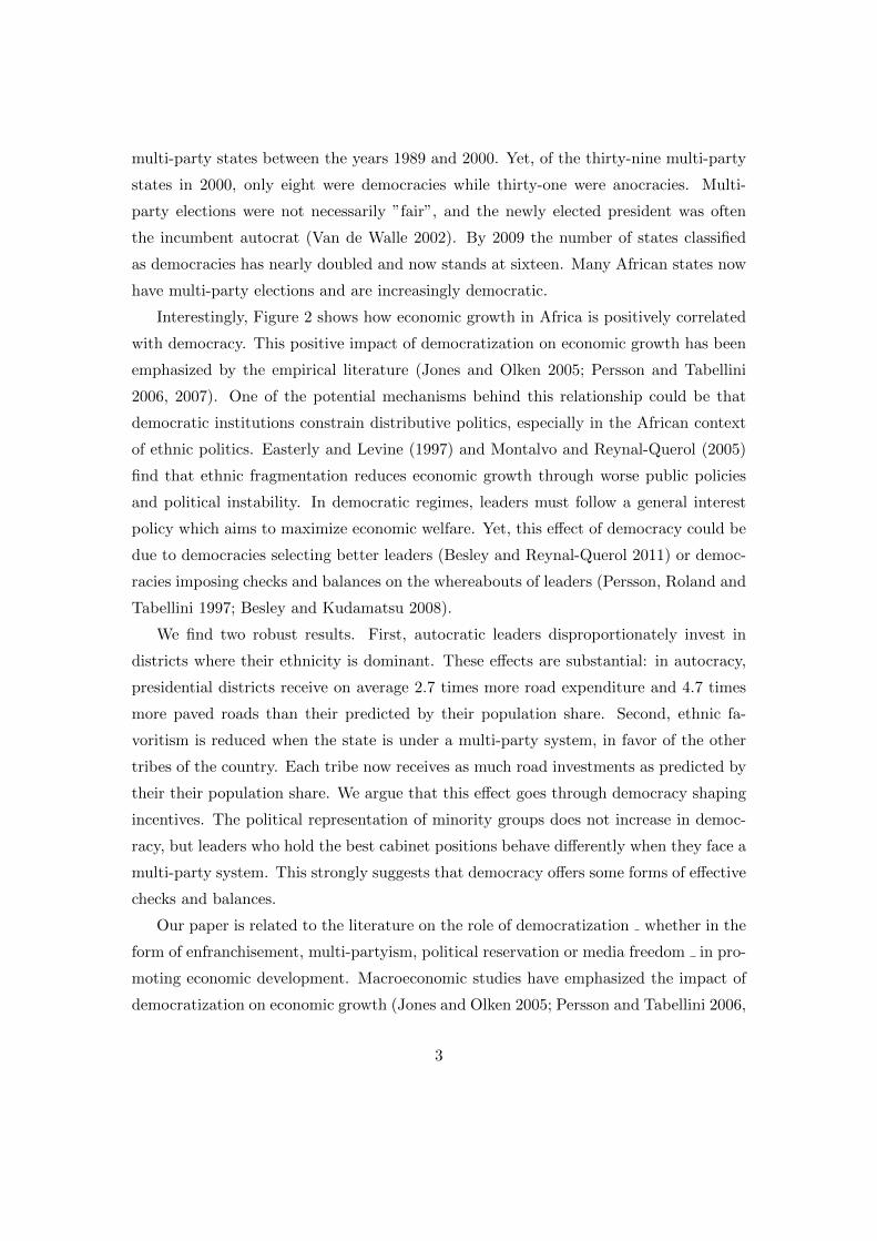
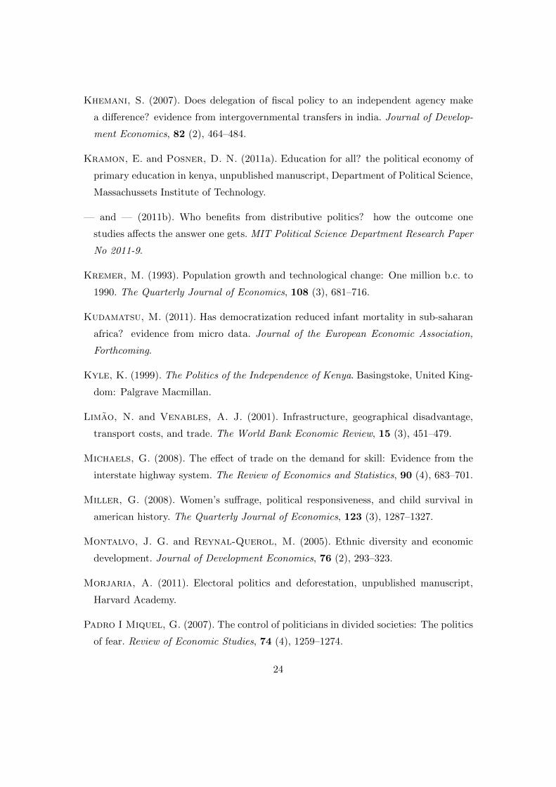
to multi-party. Figure 1 displays the evolution of the Polity IV index for the average

Sub-Saharan African country as well for Kenya. 2 The typical African country started as

an imperfect democracy or autocracy at independence, was an autocracy in the 1970s

and 1980s, before progressing towards democracy from the early 1990s. This return

to democracy was gradual. Thirty countries switched from being single-party states to

1Exceptions are Franck and Rainer (2010) and Hodler and Raschky (2010). These studies alsoinvestigate whether African presidents favor their own ethnic group, but their evidence is based oncross-country regressions, for the recent period only. Besides, we examine the impact of democratictransitions within the same leader, while Hodler and Raschky (2010) just compare democratic and non-democratic countries.

2The combined Polity score goes from -10 (hereditary monarchy) to +10 (consolidated democracy).Polity IV recommends the following classification: autocracies (-10 to -6), anocracies (-5 to +5) anddemocracies (+6 to +10).

2

multi-party states between the years 1989 and 2000. Yet, of the thirty-nine multi-party

states in 2000, only eight were democracies while thirty-one were anocracies. Multi-

party elections were not necessarily ”fair”, and the newly elected president was often

the incumbent autocrat (Van de Walle 2002). By 2009 the number of states classified

as democracies has nearly doubled and now stands at sixteen. Many African states now

have multi-party elections and are increasingly democratic.

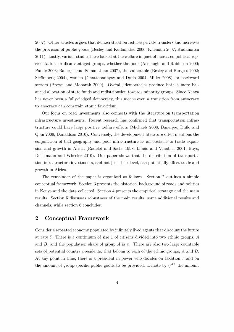
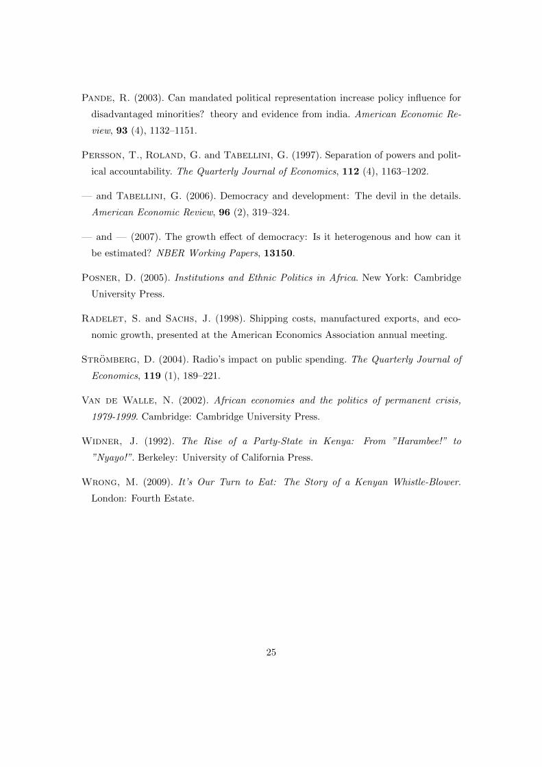
Interestingly, Figure 2 shows how economic growth in Africa is positively correlated

with democracy. This positive impact of democratization on economic growth has been

emphasized by the empirical literature (Jones and Olken 2005; Persson and Tabellini

2006, 2007). One of the potential mechanisms behind this relationship could be that

democratic institutions constrain distributive politics, especially in the African context

of ethnic politics. Easterly and Levine (1997) and Montalvo and Reynal-Querol (2005)

find that ethnic fragmentation reduces economic growth through worse public policies

and political instability. In democratic regimes, leaders must follow a general interest

policy which aims to maximize economic welfare. Yet, this effect of democracy could be

due to democracies selecting better leaders (Besley and Reynal-Querol 2011) or democ-

racies imposing checks and balances on the whereabouts of leaders (Persson, Roland and

Tabellini 1997; Besley and Kudamatsu 2008).

We find two robust results. First, autocratic leaders disproportionately invest in

districts where their ethnicity is dominant. These effects are substantial: in autocracy,

presidential districts receive on average 2.7 times more road expenditure and 4.7 times

more paved roads than their predicted by their population share. Second, ethnic fa-

voritism is reduced when the state is under a multi-party system, in favor of the other

tribes of the country. Each tribe now receives as much road investments as predicted by

their their population share. We argue that this effect goes through democracy shaping

incentives. The political representation of minority groups does not increase in democ-

racy, but leaders who hold the best cabinet positions behave differently when they face a

multi-party system. This strongly suggests that democracy offers some forms of effective

checks and balances.

Our paper is related to the literature on the role of democratization whether in the

form of enfranchisement, multi-partyism, political reservation or media freedom in pro-

moting economic development. Macroeconomic studies have emphasized the impact of

democratization on economic growth (Jones and Olken 2005; Persson and Tabellini 2006,

3

2007). Other articles argues that democratization reduces private transfers and increases

the provision of public goods (Besley and Kudamatsu 2006; Khemani 2007; Kudamatsu

2011). Lastly, various studies have looked at the welfare impact of increased political rep-

resentation for disadvantaged groups, whether the poor (Acemoglu and Robinson 2000;

Pande 2003; Banerjee and Somanathan 2007), the vulnerable (Besley and Burgess 2002;

Stromberg 2004), women (Chattopadhyay and Duflo 2004; Miller 2008), or backward

sectors (Brown and Mobarak 2009). Overall, democracies produce both a more bal-

anced allocation of state funds and redistribution towards minority groups. Since Kenya

has never been a fully-fledged democracy, this means even a transition from autocracy

to anocracy can constrain ethnic favoritism.

Our focus on road investments also connects with the literature on transportation

infrastructure investments. Recent research has confirmed that transportation infras-

tructure could have large positive welfare effects (Michaels 2008; Banerjee, Duflo and

Qian 2009; Donaldson 2010). Conversely, the development literature often mentions the

conjunction of bad geography and poor infrastructure as an obstacle to trade expan-

sion and growth in Africa (Radelet and Sachs 1998; Limao and Venables 2001; Buys,

Deichmann and Wheeler 2010). Our paper shows that the distribution of transporta-

tion infrastructure investments, and not just their level, can potentially affect trade and

growth in Africa.

The remainder of the paper is organized as follows. Section 2 outlines a simple

conceptual framework. Section 3 presents the historical background of roads and politics

in Kenya and the data collected. Section 4 presents the empirical strategy and the main

results. Section 5 discusses robustness of the main results, some additional results and

channels, while section 6 concludes.

2 Conceptual Framework

Consider a repeated economy populated by infinitely lived agents that discount the future

at rate δ. There is a continuum of size 1 of citizens divided into two ethnic groups, A

and B, and the population share of group A is π. There are also two large countable

sets of potential country presidents, that belong to each of the ethnic groups, A and B.

At any point in time, there is a president in power who decides on taxation τ and on

the amount of group-specific public goods to be provided. Denote by ηAA the amount

4

of investment in public goods that group A receives if the president belongs to group

A, and denote by ηAB the amount of investment in public goods that group A receives

if the president belongs to group B. Define ηBA and ηBB equivalently. Groups receive

linear utility from public goods.3

For simplicity, we assume that the president can only charge a lump-sum tax τ on

all citizens and cannot discriminate across groups.4 When deciding on public goods, he

is able to direct spending to his preferred districts, but only up to the constraints that

institutions impose on him. We denote by θ ∈ [1,∞) the weakness of these institutions,

and we parametrize the constrains as follows.5 A president of type j ∈ {A,B} can set

up ηAj and ηBj such that

ηAj ≤ θηBj

ηBj ≤ θηAj

obviusly only one of these constraints can be binding at any given time.

We assume that electoral institutions are also relatively weak, and the active co-

laboration of one’s co-ethnics is necessary to keep power. Given the different degress of

institutionalization we do not take a strong stance on what this co-laboration means in

practice, but it ranges from voting for the appropriate candidates to exerting violence

to prevent other ethnic groups the full exercise of their democratic rights. To capture

this in a simple way we assume that an acting president that receives the support of his

ethnic group stays in power with probability γ. If the acting president does not receive

support, he loses his position with probability 1 and an open succession takes place in

which the new ruler will belong to the same ethnic group as the ousted president with

probability γ, for 1 > γ ≥ γ > 0. Since these transitions are in many cases weakly

institutionalized and may involve coups and violence, we assume that when the ruler

does not receive the support of his group the state cannot perform its functions for a

period, while the transition is resolved.

While the presidents belong to an ethnic group, they do not particularly care about

the other members of the group. Rather, we assume that they try to maximize the

3This will allow us to deflect criticism regarding the fact that roads are durable: with linear utility,every additional patch of road provides the same utility to citizens.

4The empirical evidence is mixed, so we take this simplifying assumption. Moreover, τ here includeslegal taxes and also indirect ways of extracting rents. The assumption of no-discrimination is thereforeequivalent to assuming that the cost of rent-extraction fall equally on all citizens.

5This simple parametrization is identical to Besley and Persson (2010).

5

amount of resources they can extract. Each period, the amount of resource extraction

by a leader of group j is given by

π(τ − ηAj

)+ (1− π)

(τ − ηBj

),

which, for each group, takes into account the taxes taken in and the expenditure in

public goods.

The law of motion of public goods for group j ∈ {A,B} is as follows:

Git = Git−1 +R(ηij)

where R(.) is increasing and concave with R(0) = 0. This law of motion ignores depre-

ciation (for simplicity) and assumes that there are absortion constraints. The marginal

return to money devoted to building roads is decreasing (as prices increase, firm capac-

ities are strained, etc).

The citizens of group i receive labor income l, pay taxes τ , and enjoy public goods

Git which gives them the following simple instantaneous utility in period t:

l − τt +Git

At any point in time, this economy is in one of two payoff-relevant states, St ∈ {A,B}which capture which ethnic group the leader in power belongs to.6

The timing of the game, starting with a leader from group j ∈ {A,B} is as follows:

1. The leader announces the policy vector Pt ={τ j , ηAj , ηBj

}2. The citizens of goup j ∈ {A,B} decide whether to support the leader, st = 1 or

not st = 0

3. If st = 1, Pt is implemented and payoffs are realized. Next period starts with

St+1 = St with probability γ, and the state switches with probability 1− γ.

4. If st = 0, the leader is immediately ousted and the transition vector P = {0, 0, 0}is implemented. With probability γ the new ruler belongs to the same group as

the ousted ruler and hence St+1 = St. With probability 1 − γ the state switches

to the other group.

6There is also the possibility of using the existing road stock as a state which can complicate things.Think about this.

6

We solve this game for the Markov Perfect Equilibrium (MPE) of the game. Strate-

gies can therefore only be conditioned on the state and past play within the stage game.

We proceed by backwards induction. Suppose without loss of generality that the

state is St = A. Hence we need to examine first the decision of group A to support the

president as a function of the policy Pt ={τA, ηAA, ηBA

}that he has proposed at stage

1. To do this, it is useful to add some notation. Denote by V i(S) the value function

for a citizen of group i ∈ {A,B} in a subgame that starts in state S ∈ {A,B}. Given

the given policy vector Pt and the expected path of play given by the value functions, a

citizen of group A, if supporting (st = 1) obtains:

l − τA +GAt + δγV A(A) + δ (1− γ)V A(B).

Alternatively, if the group withdraws support (st = 0), citizens obtain:

l +GAt−1 + δγV A(A) + δ(1− γ

)V A(B).

Hence, the support condition reduces to:

τA −R(ηAA) ≤ δ(γ − γ

) (V A(A)− V A(B)

). (1)

By subgame perfection, the ruler always wants to satisfy this condition. Failing to

do so implies his immediate loss of power. Hence, when the ruler decides on the policy

to announce, he maximizes his rents subject to (1) and the insitutional constraints. His

program is therefore the following

maxτA,ηAA,ηAB

π(τA − ηAA

)+ (1− π)

(τA − ηBA

)+ δγWA

subject to

ηAA ≤ θηBA (λ)

ηBA ≤ θηAA

τA −R(ηAA) ≤ δ(γ − γ

) (V A(A)− V A(B)

)(µ)

where WA is the value of the continuation game for a president from group A. The first

order conditions of this game yield

π + 1− π = µ

−π − λ+ µR′(ηAA) = 0

− (1− π) + θλ = 0

7

So, eliminating λ, we have

µ = 1

R′(ηAA) = π +1− πθ

ηAA = θηBA

hence the institutional constraint is always binding, and public goods to the group of

the president are excessively provided if θ > 1. Indeed if θ = 1 public investment is

equally and efficiently distributed. The mathematical proof is available in appendix B.

3 Historical Background and Data

In this section, we describe the essential features of the Kenyan economy, the political

system and the data that we have collected to analyze how political regime changes

affect the allocation of public investments.

3.1 New Data on Kenya, 1889-2011

To evaluate the impact of political regime changes on the spatial allocation of public

investments, we construct a new panel data set of 41 Kenyan districts, which we track

almost annually from 1889 to 2011.7 Further details on the data collected on road

investments and ethnic politics is explained in the Data Appendix A.

We first construct a panel data set of road investments for the whole period of Kenya’s

history starting from the British colonization era. Our main variable is road development

expenditure for a district in a particular year.8 The panel data was recreated using GIS

and annual reports listing individual road projects and their related costs. Our second

key variable is the total length (km) of paved and non-paved roads at the district level.

This variable is an unbalanced panel in the time dimension as maps are not available

every year.9 The first paved road in Kenya was built in 1945. From 1955, we are also able

to distinguish improved (laterite) and dirt roads within the category of unpaved roads.

7The 41 districts correspond to the administrative decomposition of Kenya in 1963. These districtboundaries have remained stable until 1992. These districts belong to 8 provinces.

8Road expenditure can be separated into road development expenditure (investments) and road re-current expenditure (maintenance). Our data only allows us to capture road development expenditureand not maintenance at the district level. We find that 65.3% of the total 1963-2010 road expenditurewas allocated to road development expenditure.

9Our data points are 1889-1961, 1964, 1967, 1969, 1972, 1974, 1979, 1981, 1987, 1989, 1992 and 2002.

8

We have the total length (km) of paved, improved and dirt (or just unpaved) roads at

the district level for selected years. This data was also created using GIS and historical

road maps and colonial reports.10 In essence, we can track road investments in terms

of expenditure and physical building. As we exploit the variation in political regime

changes, using annual data is essential. We focus on using road development expenditure

as our main variable and we use the physical road building data to strengthen our results.

In order to investigate the ethnic favoritism dimension, we then splice our road panel

dataset with data on ethnic politics in Kenya. In particular, we construct a database

on the position, ethnicity and district of birth of cabinet members between 1963 and

2011.11 This allows us to track the representation of each ethnic group in the politics

space.12. As mentioned earlier, our unit of analysis is the district, as they are ethnically

homogenous (see appendix A figure 1). These boundaries have remained stable and were

demarcated by the British.13 Hence, we can relate changes in the ethnicity of political

leaders and changes in the spatial allocation of road investments.

3.2 Road Investments in Kenya

Road expenditure are the single largest item in terms of public investments. They

represented 15.2% of the total 1963-2010 development budget. By comparison, other

public investments such as education, health and water respectively received 5.5%, 5.7%

and 6.5% of the total development expenditure budget.14

The Kenya system of road funding has been centralized for most of the period of

study, with Provincial and District Commissioners passing up requests for projects to

the Ministry of Public Works.15 The Ministry of Public Works deals with those requests

and prepares a national strategy for road building. The Ministry of Finance then over-

10As detailed in Data Appendix A, the Kenyan government has not conducted a road survey since2002.

11We have data for all the election years. Elections for the National Assembly took place even duringsingle-party autocracy years to renew the tenure of the members of parliament. Of course, all candidatesbelonged to and were from the single-party.

12We use classification of ethnic groups from the population census, see appendix A table 213Further, the ethnic population census for the years 1948, 1962, 1969, 1979, 1989, 2003 and 2009

show stability in the ethnic group shares over time (see appendix A table 3).14The respective shares of roads, education, health and water are not significantly different in single-

party autocracy versus multi-party democracy.15The Ministry of Public Works has been in charge with planning and building roads, except in 1979-

1988 when it was under the Ministry of Transport & Communications, and also during 2008-2011 whena specific Ministry of Roads was setup.

9

sees and resolves competing claims from the different Ministries and overall oversight

is exercised by the Office of the President. Barkan and Chege (1989) provides a good

description of the system. In essence, Provincial Commissioners were nominated by the

Office of the President, which guaranteed their loyalty by rewarding them with unlimited

authority on their province. As a result, a disproportionate share of provincial and dis-

trict commissioners were coming from the ethnic group of the president and this ensured

that power remained highly centralized.16

Figure 3 depicts the evolution of the road network from 1890 to 2002. The first

motor roads were built as feeder roads for the Uganda Railway, constructed in 1901

from Mombasa to exploit the resources of Uganda. This permitted British settlers to

capture the most fertile land of both the now Central Province and Rift Valley to grow

tea and coffee for exports. Those areas the White Highlands had 17.7 times more

Europeans per sq km than the rest of Kenya. They were also producing 27.1 times more

coffee and 60.7 times more tea, and had 13.0 times more paved roads, per sq km. This

concentration of the road network at independence is confirmed by appendix A figure

2, which displays the White Highlands, the main network in 1963 and cities in 1962.

Additional roads were then built to connect the main regions and towns of the country

for administrative purpose. After independence, the road network was dramatically

extended and upgraded, with the objectives of promoting trade (e.g., cash crop exports),

tourism and helping rural settlements. In total, the total length of Kenya’s road network

increased from 12,808 km in 1964 to 22,628 km in 2002. 54% of this expansion was driven

by paved roads, 36% by improved roads and 10% by tracks.

3.3 Ethnic Politics

To test whether road placement is driven by political motives, we need to understand

in whose hands the power is vested. The general elections of May 1963 between the

two main political parties, took place a few months before Kenya’s independence and

saw KANU (Kenyan African National Union) beat KADU (Kenyan African Democratic

Union). Jomo Kenyatta became president and his tribe, the Kikuyus obtained 31.6%

16Barkan and Chege (1989) write (p.439): ”Although the P.C.s and D.C.s [provincial and districtcommissioners] were responsible for the administration of all government policies in their areas, theirprimary tasks were to maintain law and order, and to facilitate the work of staff posted to each provinceand district by the ministry which gave them their orders. Policy, in short, was determined at the centre,albeit coordinated in the field by the team led by the P.C.”

10

of the cabinet positions although they represented only 18.8% of the population.17 In

November 1964, KADU merged with KANU in order to assist a consolidated effort

towards decolonization. Kenya becomes a de jure multi-party democracy, until March

1966 when the Luos creates their own party, KPU (Kenya People’s Union). Kenyatta,

feeling betrayed, uses the state apparel to pursue his opponents, and the main KPU

leader is arrested.18. Kenya as a result becomes a single-party autocracy, this transition

was typical of African countries during that period (see figure 1). During Kenyatta’s

tenure, the Kikuyus were said to receive most public investments (Barkan and Chege

1989; Wrong 2009).

When Kenyatta dies of natural causes in August 1978, he is replaced by his vice-

president, Daniel Arap Moi, a Kalenjin. Prominent Kikuyu leaders oppose this transition

and demand a constitutional change allowing them to elect another Kikuyu president.

Moi however secures the support of other tribes and factious Kikuyus from the ruling

party, which he rewards with cabinet positions (see Widner 1992, p.110-129). Moi quickly

becomes as powerful and authoritarian as Kenyatta, favoring his own people in terms

of public spending (Barkan and Chege 1989; Wrong 2009). In December 1992, facing

pressure by international donors keen on fighting corruption since the end of the Cold

War, he accepts multi-party democracy. This democratic transition is also part of a

general movement in Sub-Saharan Africa (see figure 1).

In December 2002, Moi is constitutionally barred from running again, and a coalition

of opposition parties wins the elections. Mwai Kibaki, a Kikuyu, becomes president, and

it is again argued that Kikuyus are disproportionately favored (Wrong 2009). He is re-

elected in December 2007 against a Luo candidate, but Kibaki is accused of having rigged

the elections. The first months of 2008 are characterized by ethnic riots, and an unity

government is formed in May 2008.

In essence we exploit variation in three leadership changes and within these leader-

ship changes two political institutional changes. There have been three presidents since

independence in 1963, Kenyatta (a Kikuyu) from 1963 to 1978, Moi (a Kalenjin) from

1979 to 2002 and Kibaki (a Kikuyu) from 2003 to 2011. Two of these presidents have

17Having been detained from 1953 by the British, Kenyatta had become a hero of independence anda natural candidate for presidency (see Widner 1992, p.51-52). Yet, Kyle (1999) describes how the Luoleader Tom Mboya could have emerged as the first leader of Kenya, thanks to his charisma and closelinks with the British (see p.69-90).

18KPU is banned in November 1969 (see Widner 1992, p.69-70)

11

experienced a regime change: from multi-party democracy to single-party autocracy

(Kenyatta in 1969), and from single-party autocracy to multi-party democracy (Moi in

1992). Leadership changes can be said to have been plausibly exogenous, whether orig-

inating from independence, death by natural causes or constitutional rules.19 Regime

changes were also plausibly exogenous, as part of the continent’s dynamic or imposed

from abroad.20 We exploit these changes to understand the impact of institutions on

ethnic favoritism.

4 Empirical Strategy and Main Results

In this section we describe our empirical strategy to look at whether ethnic favoritism

occurs at the district level, we also provide some graphical evidence to corroborate our

strategy and display the main empirical results.

4.1 Empirical Strategy

Assuming a population is a good measure of development and how roads should be

allocated, we construct a simple index of road favoritism21: Rpopd,t is defined as the

share of road investments going to district d in year t divided by the population share

of district d in 1962.22 If the index takes a value of one, this indicates that the district

receives as much road investments as its population share in the population of Kenya.

An index above one indicates that the district is favored in terms of road investments.

Our baseline method is to run panel data regressions for districts d and years t of the

following form:

Rpopd,t = γd + αt + βPresdistd,t + δ(Presdistd,t ×Multipartyt) + θtXd + ud,t (2)

where Rpopd,t is the road favoritism index, which can be constructed using either road

development expenditure or paved road building. Presdistd,t is a dummy equal to one

if more than 50% of district d’s population is from the ethnic group of the president in

19Likewise, an ethnic pattern of power Kikuyu-Kalenjin-Kikuyu emerged.20The fact that the leader did not change, just the regime, is a major reason why studying the Kenyan

context is very useful to identify the impact of regime changes.21An old economic history literature uses population as a measure of development (Bairoch 1988) as

well as more recent works by Kremer (1993) and Acemoglu et al. (2002).22We use the 1962 population census as future population growth could be influenced by ethnic politics.

12

year t.23 Multipartyt is a dummy equal to one if year t is a year during the multi-party

era. As such, β captures the effect of being a presidential district on road investments

in single-party autocracy, while β + δ captures this effect in multi-party democracy. γd

and αt are district and year fixed effects respectively and Xd is a vector of baseline

demographic, economic and geographic variables that might affect road placement.24

Since controlling variables Xd are included in the fixed effects γd, we allow their effect

θt to be time-varying. Lastly, ud,t are individual disturbances clustered at the district

level. Our main analysis focuses on road expenditure during 1963-2011.25

4.2 Descriptive Evidence

We first display the data we have put together to see if simple graphs indicate that

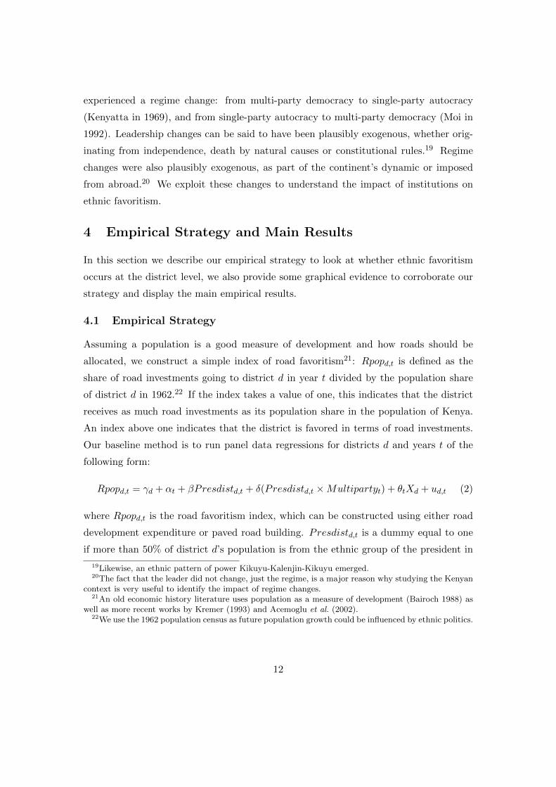
presidents practice ethnic favoritism. Figure 3 shows the evolution of the road network

and highlight the Kikuyu and Kalenjin home districts. Kenyatta, a Kikuyu is president

between the years 1963 and 1978. When comparing the 1964 and 1979 maps, we see

much more paved roads in Kikuyu areas, with most of paved road investments occurring

after 1969, during the autocracy era. Moi, a Kalenjin is president between 1979 and

2002. If one compares the 1979 and 2002 maps, we see more roads in the Kalenjin areas

and most of these roads were built prior to 1992, during the autocracy era.

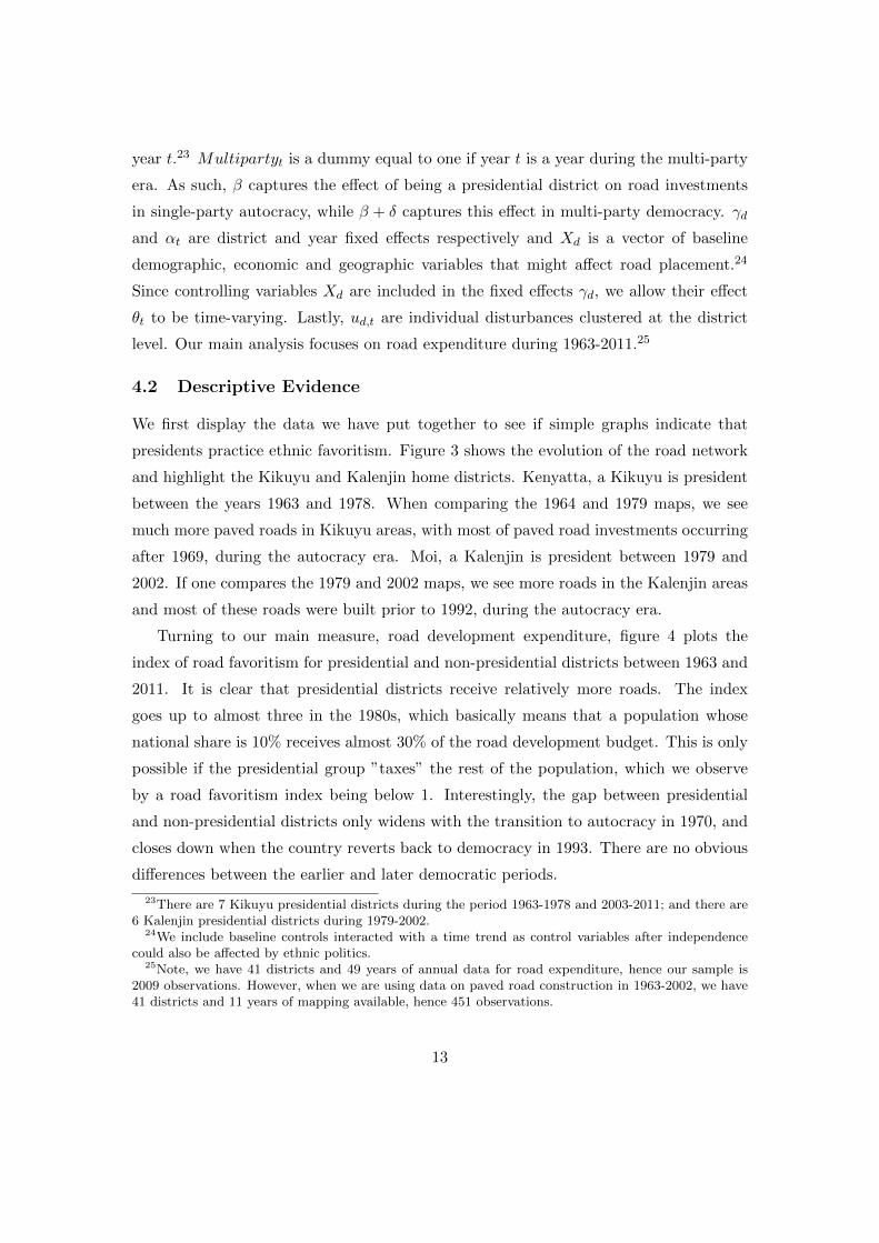
Turning to our main measure, road development expenditure, figure 4 plots the

index of road favoritism for presidential and non-presidential districts between 1963 and

2011. It is clear that presidential districts receive relatively more roads. The index

goes up to almost three in the 1980s, which basically means that a population whose

national share is 10% receives almost 30% of the road development budget. This is only

possible if the presidential group ”taxes” the rest of the population, which we observe

by a road favoritism index being below 1. Interestingly, the gap between presidential

and non-presidential districts only widens with the transition to autocracy in 1970, and

closes down when the country reverts back to democracy in 1993. There are no obvious

differences between the earlier and later democratic periods.

23There are 7 Kikuyu presidential districts during the period 1963-1978 and 2003-2011; and there are6 Kalenjin presidential districts during 1979-2002.

24We include baseline controls interacted with a time trend as control variables after independencecould also be affected by ethnic politics.

25Note, we have 41 districts and 49 years of annual data for road expenditure, hence our sample is2009 observations. However, when we are using data on paved road construction in 1963-2002, we have41 districts and 11 years of mapping available, hence 451 observations.

13

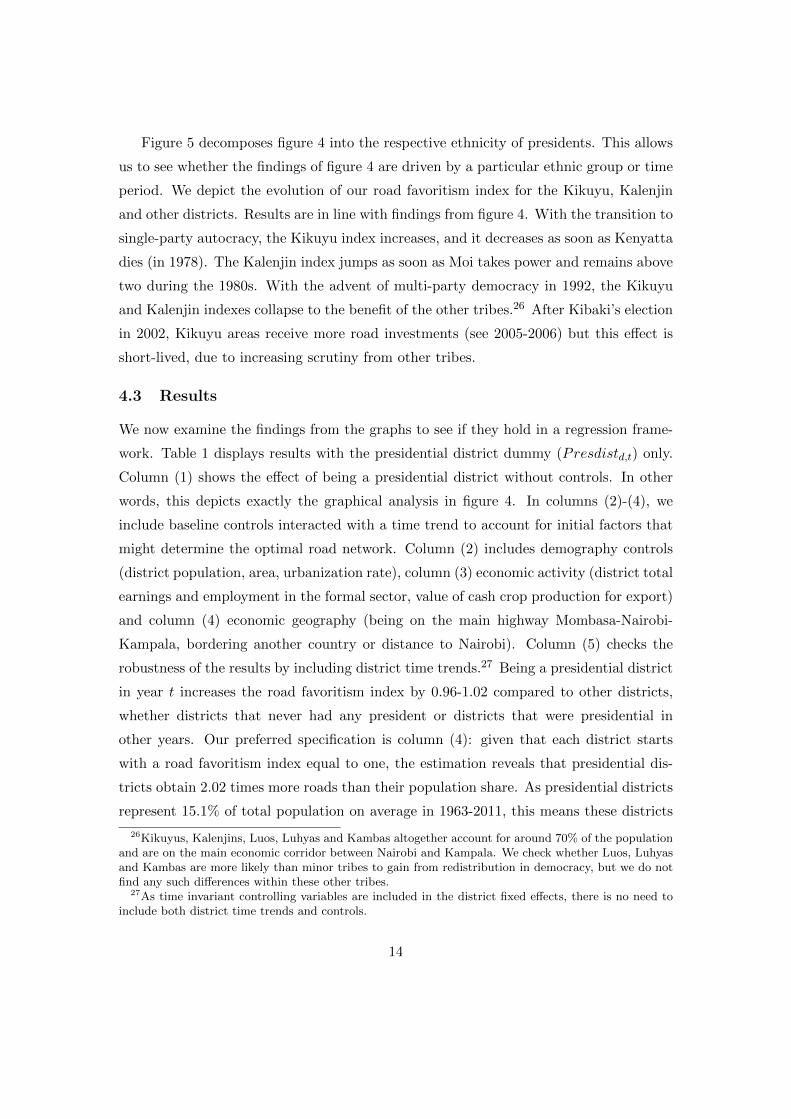
Figure 5 decomposes figure 4 into the respective ethnicity of presidents. This allows

us to see whether the findings of figure 4 are driven by a particular ethnic group or time

period. We depict the evolution of our road favoritism index for the Kikuyu, Kalenjin

and other districts. Results are in line with findings from figure 4. With the transition to

single-party autocracy, the Kikuyu index increases, and it decreases as soon as Kenyatta

dies (in 1978). The Kalenjin index jumps as soon as Moi takes power and remains above

two during the 1980s. With the advent of multi-party democracy in 1992, the Kikuyu

and Kalenjin indexes collapse to the benefit of the other tribes.26 After Kibaki’s election

in 2002, Kikuyu areas receive more road investments (see 2005-2006) but this effect is

short-lived, due to increasing scrutiny from other tribes.

4.3 Results

We now examine the findings from the graphs to see if they hold in a regression frame-

work. Table 1 displays results with the presidential district dummy (Presdistd,t) only.

Column (1) shows the effect of being a presidential district without controls. In other

words, this depicts exactly the graphical analysis in figure 4. In columns (2)-(4), we

include baseline controls interacted with a time trend to account for initial factors that

might determine the optimal road network. Column (2) includes demography controls

(district population, area, urbanization rate), column (3) economic activity (district total

earnings and employment in the formal sector, value of cash crop production for export)

and column (4) economic geography (being on the main highway Mombasa-Nairobi-

Kampala, bordering another country or distance to Nairobi). Column (5) checks the

robustness of the results by including district time trends.27 Being a presidential district

in year t increases the road favoritism index by 0.96-1.02 compared to other districts,

whether districts that never had any president or districts that were presidential in

other years. Our preferred specification is column (4): given that each district starts

with a road favoritism index equal to one, the estimation reveals that presidential dis-

tricts obtain 2.02 times more roads than their population share. As presidential districts

represent 15.1% of total population on average in 1963-2011, this means these districts

26Kikuyus, Kalenjins, Luos, Luhyas and Kambas altogether account for around 70% of the populationand are on the main economic corridor between Nairobi and Kampala. We check whether Luos, Luhyasand Kambas are more likely than minor tribes to gain from redistribution in democracy, but we do notfind any such differences within these other tribes.

27As time invariant controlling variables are included in the district fixed effects, there is no need toinclude both district time trends and controls.

14

obtained on average around 30.5% of the total road expenditure budget.

We now seek to understand how this ethnic favoritism changes across political regimes

by exploiting changes in the political system from democracy-to-autocracy-to-democracy.

In Table 2, we include the presidential district dummy (Presdistd,t) and its interaction

with the multi-party year dummy (Presdistd,t × Multipartyt) to capture the transi-

tions. Note we also include the multi-party dummy, but the interpretation of its effect

is complicated by the presence of the year fixed effects. Specifications in table 2 mir-

ror exactly table 1. Results without controls are reported in column (1), results with

controls in columns (2)-(4) and results with district time trends are reported in column

(5). Being a presidential district in autocratic years increases the road favoritism index

by 1.56-1.74 compared to other districts, while this effect is reduced by 1.08-1.32 in

democratic years.28 Interestingly, one cannot reject the null hypothesis that the effect

of democracy is eliminating the effect of being a presidential district, as indicated by the

F-test in the last row. These findings are robust to including more controls or district

time trends. Given each district starts with a road favoritism index equal to one, presi-

dential districts obtain 2.74 times more roads than their population share in autocratic

years (column (4)). This implies that presidential districts have obtained on average

41.4% of the road development expenditure over the period.

In table 3, we check the robustness of our findings. Our main results are reproduced

in column (1) and column (2). Our main outcome variable to measure road favoritism

has been road expenditure share benchmarked to the population share of that district.

Another plausible benchmark to consider is the share of road expenditure going to district

d in year t divided by the area share of that district. We find that presidential districts

receive 4.05 times more roads than their area share (see column (4)).29 In columns (5)

and (6) - specification in columns (1) and (2) is replicated however this time using our

complementary data set on physical road building, in particular paved road construction.

As discussed before, our road construction panel is unbalanced in the time dimension

due to the lack of frequent maps. Although results are less precisely estimated, they give

a similar picture to what we obtain with road expenditure. In autocracy, paved road

28Dropping year fixed effects does not affect the presidential effects but it permits us to interpret thecoefficient of the multi-party dummy. We find that the road favoritism index increases by 0.13-0.21in democracy for each district (results available upon request). This is logical since the president inautocracy cannot favor his own group without taxing other tribes.

29We obtain similar results if we standardize by population density (results available upon request).

15

investments received by presidential districts are 4.71 times their population share (see

column (1)). This means they have obtained on average 71.1% of paved road construction

over the period. But this effect is strongly reduced in democracy and we cannot reject the

hypothesis that democracy is reducing this effect. Why is the autocracy effect larger for

paved road construction (3.71, see table 3 - column 6) than for road expenditure (1.74,

see table 3 - column 2)? Paved roads are respectively 6.7 and 20 times more expensive

than improved and dirt roads (Alexeeva et al. 2008), but road expenditure includes all

types of roads. If the president only favors his ethnic group with the most expensive type

of roads, paved roads, and other districts with improved and dirt roads, the presidential

effect will be attenuated for road expenditure. We are unable to directly verify this

hypothesis as we cannot separate out road expenditure across the different road types.

It is however clear from the previous analysis that the president discriminates groups

both in terms of road quantity and quality. In columns (7) and (8), similar specification

to column (3) and (4) is replicated to see if results are robust to area share instead

of population share. The results are in line with previous findings using both different

outcome measures as well as standardizations.

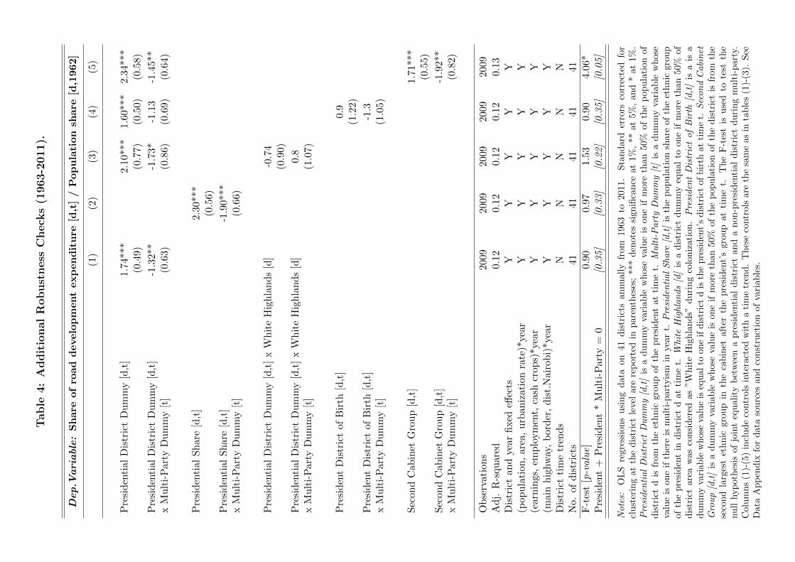
Table 4 presents various additional checks to our main results. In column (1), we

replicate our main finding. In column (2), instead of having a discrete measure of

whether a district is presidential, we test the district population share of the president’s

ethnic group. The effects are larger as these are being identified on districts that have

a high population share aligned to the president’s ethnic group.30 One could argue

that colonization explains the geography of both politics and road investments.31 We

interact our effects with a dummy equal to one if the district is in the White Highlands,

but results are similar for districts that are not in the White Highlands (see column

(3)). In column (4), we try to see if the president’s district of birth receives more road

investments than other districts. We interact a district dummy which equals to one if

it is the district of birth of the president with a year dummy equal one if it belongs to

the multi-party era. We find a larger but not significant effect. Lastly, we investigate in

column (5) whether coalition partners receive more road investments. The core issue is

to identify coalition partners. We identify this group by using cabinet data and we create

30Recall - 5 out of 7 Kikuyu districts and 3 out of 6 Kalenjin districts have a presidential share higherthan 75%.

315 out of 7 Kikuyu districts and 2 out 6 Kalenjin districts belonged to the former White Highlands.

16

a dummy equal to one if more than 50% of district population is from the second group

in the cabinet (the presidential group being the first group). The effects for presidential

districts are larger since we now compare them with non-presidential districts that do

not belong to the second group. We find that the second group also receives more road

investments in autocracy.32

In table 5, we breakdown our data into different time periods according to the history

of Kenya. This is necessary, as the concern could be that all our findings are driven by

a particular leadership period. As before, we regress our main outcome variable, the

road favoritism index (Rpopd,t) on district dummies which take the value one if more

than 50% of the district’s population is Kikuyu or Kalenjin, the two presidential ethnic

groups. The comparison districts are other non-Kikuyu-non-Kalenjin districts. We find

that during the colonial era (column 1), Kalenjin districts received more investments.

This is not surprising because parts of the Rift Valley where the Kalenjin and Kikuyu

groups reside are located in the former White Highlands, which had been settled by

the White farmers. A Kikuyu president only has a positive and significant impact on

road investments in Kikuyu districts in the single-party era (column (2.b)). Conversely,

a Kalenjin president only has a positive and significant impact on road investments in

Kalenjin districts in the single-party (see column (3.a)). Neither presidents are able to

mobilize road investments to their ethnic homelands during the multi-party era.

5 Other Results and Channels

We verified our ethnic favoritism results as being robust to various checks. In this section

we provide additional results and explore channels through which democracy constrains

distributive politics. All the following results are presented in Appendix C. In Appendix

C Table 1, we investigate whether the influence of control variables changes over time.

For instance, it could be rational to build roads around Nairobi (the capital) first, and

later extend road building to the rest of the country. The negative effect of distance to

Nairobi would decrease over time and we would fail to capture it by interacting it with a

linear time-trend. Hence, we run the same specification but we now also interact control

variables with a time trend and its square. Results are unaffected (compare columns

32We find non-significant results of the second group effects for paved roads, despite similar pointestimates. This could be due to the fact that we have less observations for this data set. Results areavailable upon request.

17

(1) and (2)). We could imagine that Kikuyu and Kalenjin areas have already received

a large amount of investments before 1992 and hence the return of new investments is

low. We would then confound the effect of the return to democracy and regression to

the mean. On the other hand presidents could be insensitive to the economic returns of

investments, and decide to upgrade the network (paving, more lanes) in congested areas.

We run our baseline specification as before but this time we include the number of years

a district has been a presidential district. Results are unaffected (compare columns (1)

and (3)). Another typical concern in such empirical work is if observations are spatially

correlated, as then estimated standard errors are incorrect. If neighboring observations

positively influence each other, estimated standard errors are too low, and we could

mistakenly consider a insignificant coefficient as being significant. Our results are robust

to clustering standard errors at a higher spatial level, whether at the ethnic group level

(13 clusters), the province level (8 clusters), or correcting for spatial autocorrelation

using standard methods (see columns (4), (5) and (6)).33

Lastly, we make sure that the presidential group does not receive more transfers

because it also pays more taxes. We want to ensure the president provides her own

group with net benefits. As argued by Padro I Miquel (2007), groups cannot be directly

discriminated using taxes. But the state can tax differently sectors associated with

specific ethnic groups. In many African countries, a large share of the budget is financed

by taxes on the cash crop sector. We thus investigate if the president taxes differently

the crop in which her own group is specialized. Using production data at the district

level in 1965 for coffee and tea, the two main exports of Kenya, we find that coffee

is mainly a Kikuyu crop while tea is mostly a Kalenjin crop.34 We test whether the

president, Kikuyu or Kalenjin, taxes more (or less) her own group rather than the other

group, in a democracy versus an autocracy. We regress the yearly taxation rate on a

dummy if it is the crop of the president (coffee when Kikuyu, tea when Kalenjin) and its

interaction with the multi-party dummy, including time and crop fixed effects and a crop

time trend. Results show that there is no effect of being the presidential group on the

33The cluster covariance matrix approach is to cluster observations so that group-level averages areindependent. As demonstrated by Bester et al. (2011), clustering observations at a higher spatial levelcan ensure spatial independence. The plug-in HAC covariance matrix approach is to plug-in a covariancematrix estimator that is consistent under heteroskedasticity and autocorrelation of unknown form. Thisapproach models spatial dependence instead of time dependence, and has been popularized by Conley(1999).

3469.6% of coffee is produced by Kikuyu districts, and 87.8% of tea by Kalenjin districts.

18

relative taxation rate of her own group. We cannot reject the hypothesis that presidents

are not taxing more (or less) their own crop, whether in autocracy or democracy.35

Autocrats only discriminate groups using transfers, not taxes, which confirms that road

investments are net benefits.36

We now explore the results we had found of the second group effects (Table 4 column

(5)). These set of results are presented in Appendix C Table 2. Another plausibly

definition of the second important group is to use the ethnicity of the vice-president.

There have been 11 vice-presidents during the history of Kenya (1964 and 2011) and

all of them have been from a different ethnic group than their president. Districts that

share the ethnicity of the vice-president receives more roads, but this effect is strongly

reduced in democracy (column 2). Instead of considering the second group in the cabinet

using all cabinet positions, we restrict our cabinet sample to the president and the top

ten positions in terms of investment budget (column 3), or the president and the top

ten positions using the hierarchy available in the official government list (column 4).

Our second group effects are robust to those definitions. We run the same baseline

specification as before except that we have as the variable of interest the cabinet share in

year t of the majoritarian ethnic group in the district. We find a positive and significant

effect of cabinet share in autocracy, which is then dampened in democracy. But those

effects disappears when we include the president and second group effects. This means

the cabinet shares do not matter per se, but the cabinet rank (president, second group)

does (column 5). Lastly, we do not find any effect for the ethnicity or district of birth

of the minister in charge for road building (column 6).

5.1 Channels and Discussion of the Results

One possible mechanism that could help in distributing ethnic favoritism is through

cabinet appointments. We examine if democracy affects the distribution of cabinet posi-

tions across the presidents and other ethnic groups. Our data set consists of the cabinet

35Results not reported here but available upon request. This non-result contradicts the claim madeby Kasara 2007 that African presidents have taxed more their own group.

36Another issue is whether such results can be generalized to other public goods (Kramon and Posner2011b). Yet, Barkan and Chege (1989), Franck and Rainer (2010) and Kramon and Posner (2011b) haveshown that co-ethnics of the president in Kenya were more likely to receive public investments in theirhealth infrastructure, have some primary education, be literate, have access to water, while no positive(or negative) presidential effect was found for infant mortality, vaccinations and access to electricity.Overall, net benefits for co-ethnics were clearly positive.

19

share of the 13 ethnic groups for all the election years. We run the same specification

as before except we consider the dependent variable as the cabinet share of each ethnic

group in year t divided by its population share in 1962. An index higher than one means

an ethnic group is receiving more cabinet positions than its ethnic national population

share. We then regress this index on a district dummy which equals one if it is the ethnic

group of the president, as well as its interaction with the multi-party dummy, including

ethnic group, time fixed effects and an ethnic group time trend. Results are presented

in Appendix C Table 3. We find that the presidential group receives 1.64 more cabinet

positions than its population share (column (1)). When we alternatively use cabinet

shares based on top fiscal positions, we find that the presidential group receives 2.28

times more cabinet positions than its population share, which shows the president re-

wards her people with the best positions (column (2) and (3)).37 Interestingly, those

effects are not modified in democracy. We also find that the second group is not signifi-

cantly more or less represented in democracy. If anything, the structure of the cabinet

(presidential, second and other tribes) does not change with democracy (columns (4),

(5) and (6)).

Although we cannot empirically assess which component of democracy (end of repres-

sion, enfranchisement, multipartism, media freedom, etc.) drive our results, our work

has four major empirical results which we can directly relate to our conceptual frame-

work. First, the president strongly rewards her people in autocracy. Yet, Kenya being

a divided country with various small ethnic groups, the presidential group is unlikely to

remain in power without retributing another group. The fact that the second group in

the cabinet receives some roads, although the effect is smaller and less robust, supports

this hypothesis. Second, democracy implies universalism in our context, as each group

is then receiving as much road investments as its population share. Third, the fact that

the same leader behaves differently when they face a multi-party system shows that the

positive effects of democracy are not just about the selection of good leaders. Lastly,

the structure of the cabinet does not change in democracy and the cabinet share has

no impact once we control for the cabinet ranking of ethnic groups (president, second

group, other groups). Democracy does not increase political representation for minority

groups, but constrains the power associated with the best cabinet positions. The third

37Given an average population share of 15.2% in 1963-2010, this indicates the presidential groupobtains 24.9% of cabinet positions and 34.7% of the best cabinet positions.

20

and fourth findings indicate that democracies offer effective checks and balances which

constrain the powers of bad leaders.

6 Conclusion

We assembled a unique dataset on road investments and exploited political variations

in Kenya’s history to understand the extend of ethnic favoritism. We find that leaders

disproportionately favor their own people in autocracy. The presidential group receives

2.7 times more road investments than its population share. This goes up to 4.7 times

more if we consider paved road construction. The second group in the cabinet also

receives some roads, although the effect is smaller and less robust. Those effects are

strongly reduced in democracy, to the profit of the other tribes of the country. The

introduction of democracy implies universalism, as a result each group receives as much

road investments as its population share.

We argue that this effect goes through democracy shaping incentives. The political

representation of minority groups does not increase in democracy, but leaders who hold

the best cabinet positions behave differently when they face a multi-party system. This

strongly suggests that democracy, even when it is imperfect, offers some effective checks

and balances. This must be kept in mind, as Africa engages on the path of democracy.

21

References

Acemoglu, D., Johnson, S. and Robinson, J. A. (2002). Reversal of fortune: Ge-

ography and institutions in the making of the modern world income distribution. The

Quarterly Journal of Economics, 117 (4), 1231–1294.

— and Robinson, J. A. (2000). Why did the west extend the franchise? democracy,

inequality, and growth in historical perspective. The Quarterly Journal of Economics,

115 (4), 1167–1199.

Alexeeva, V., Padam, G. and Queiroz, C. (2008). Contracts and unit costs for

enhanced governance in sub-saharan africa. World Bank Transport Papers, (21).

Bairoch, P. (1988). Cities and Economic Development: Frow the Dawn of History to

the Present. Chicago: The University of Chicago Press.

Banerjee, A., Duflo, E. and Qian, N. (2009). On the road: Access to transportation

infrastructure and economic growth in china, unpublished manuscript, Department of

Economics, Massachussets Institute of Technology.

— and Somanathan, R. (2007). The political economy of public goods: Some evidence

from india. Journal of Development Economics, 82 (2), 287–314.

Barkan, J. D. and Chege, M. (1989). Decentralising the state: District focus and

the politics of reallocation in kenya. The Journal of Modern African Studies, 27 (03),

431–453.

Besley, T. and Burgess, R. (2002). The political economy of government responsive-

ness: Theory and evidence from india. The Quarterly Journal of Economics, 117 (4),

1415–1451.

— and Kudamatsu, M. (2006). Health and democracy. American Economic Review,

96 (2), 313–318.

— and — (2008). Making autocracy work. In E. Helpman (ed.), Institutions and Eco-

nomic Performance, Cambridge MA: Harvard University Press.

— and Reynal-Querol, M. (2011). Do democracies select more educated leaders?

American Political Science Review, 105 (3).

22

Bester, A., Conley, T. and Hansen, C. (2011). Inference with dependent data using

cluster covariance estimators. Journal of Econometrics, Forthcoming.

Brown, D. S. and Mobarak, A. M. (2009). The transforming power of democracy:

Regime type and the distribution of electricity. American Political Science Review,

103 (02), 193–213.

Buys, P., Deichmann, U. and Wheeler, D. (2010). Road network upgrading and

overland trade expansion in sub-saharan africa. Journal of African Economies, 19 (3),

399–432.

Chattopadhyay, R. and Duflo, E. (2004). Women as policy makers: Evidence from

a randomized policy experiment in india. Econometrica, 72 (5), 1409–1443.

Conley, T. G. (1999). Gmm estimation with cross sectional dependence. Journal of

Econometrics, 92 (1), 1–45.

Donaldson, D. (2010). Railroads of the Raj: Estimating the Impact of Transportation

Infrastructure. NBER Working Papers 16487, National Bureau of Economic Research,

Inc.

Easterly, W. and Levine, R. (1997). Africa’s growth tragedy: Policies and ethnic

divisions. The Quarterly Journal of Economics, 112 (4), 1203–50.

Franck, R. and Rainer, I. (2010). Does the leader’s ethnicity matter? ethnic fa-

voritism, education and health in sub-saharan africa, unpublished manuscript, De-

partment of Economics, Bar Ilan University.

Hodler, R. and Raschky, P. A. (2010). Foreign Aid and Enlightened Leaders. Work-

ing Papers 10.05, Swiss National Bank, Study Center Gerzensee.

Jones, B. F. and Olken, B. A. (2005). Do leaders matter? national leadership and

growth since world war ii. The Quarterly Journal of Economics, 120 (3), 835–864.

Kasara, K. (2007). Tax me if you can: Ethnic geography, democracy, and the taxation

of agriculture in africa. The American Political Science Review, 101 (1), pp. 159–172.

23

Khemani, S. (2007). Does delegation of fiscal policy to an independent agency make

a difference? evidence from intergovernmental transfers in india. Journal of Develop-

ment Economics, 82 (2), 464–484.

Kramon, E. and Posner, D. N. (2011a). Education for all? the political economy of

primary education in kenya, unpublished manuscript, Department of Political Science,

Massachussets Institute of Technology.

— and — (2011b). Who benefits from distributive politics? how the outcome one

studies affects the answer one gets. MIT Political Science Department Research Paper

No 2011-9.

Kremer, M. (1993). Population growth and technological change: One million b.c. to

1990. The Quarterly Journal of Economics, 108 (3), 681–716.

Kudamatsu, M. (2011). Has democratization reduced infant mortality in sub-saharan

africa? evidence from micro data. Journal of the European Economic Association,

Forthcoming.

Kyle, K. (1999). The Politics of the Independence of Kenya. Basingstoke, United King-

dom: Palgrave Macmillan.

Limao, N. and Venables, A. J. (2001). Infrastructure, geographical disadvantage,

transport costs, and trade. The World Bank Economic Review, 15 (3), 451–479.

Michaels, G. (2008). The effect of trade on the demand for skill: Evidence from the

interstate highway system. The Review of Economics and Statistics, 90 (4), 683–701.

Miller, G. (2008). Women’s suffrage, political responsiveness, and child survival in

american history. The Quarterly Journal of Economics, 123 (3), 1287–1327.

Montalvo, J. G. and Reynal-Querol, M. (2005). Ethnic diversity and economic

development. Journal of Development Economics, 76 (2), 293–323.

Morjaria, A. (2011). Electoral politics and deforestation, unpublished manuscript,

Harvard Academy.

Padro I Miquel, G. (2007). The control of politicians in divided societies: The politics

of fear. Review of Economic Studies, 74 (4), 1259–1274.

24

Pande, R. (2003). Can mandated political representation increase policy influence for

disadvantaged minorities? theory and evidence from india. American Economic Re-

view, 93 (4), 1132–1151.

Persson, T., Roland, G. and Tabellini, G. (1997). Separation of powers and polit-

ical accountability. The Quarterly Journal of Economics, 112 (4), 1163–1202.

— and Tabellini, G. (2006). Democracy and development: The devil in the details.

American Economic Review, 96 (2), 319–324.

— and — (2007). The growth effect of democracy: Is it heterogenous and how can it

be estimated? NBER Working Papers, 13150.

Posner, D. (2005). Institutions and Ethnic Politics in Africa. New York: Cambridge

University Press.

Radelet, S. and Sachs, J. (1998). Shipping costs, manufactured exports, and eco-

nomic growth, presented at the American Economics Association annual meeting.

Stromberg, D. (2004). Radio’s impact on public spending. The Quarterly Journal of

Economics, 119 (1), 189–221.

Van de Walle, N. (2002). African economies and the politics of permanent crisis,

1979-1999. Cambridge: Cambridge University Press.

Widner, J. (1992). The Rise of a Party-State in Kenya: From ”Harambee!” to

”Nyayo!”. Berkeley: University of California Press.

Wrong, M. (2009). It’s Our Turn to Eat: The Story of a Kenyan Whistle-Blower.

London: Fourth Estate.

25

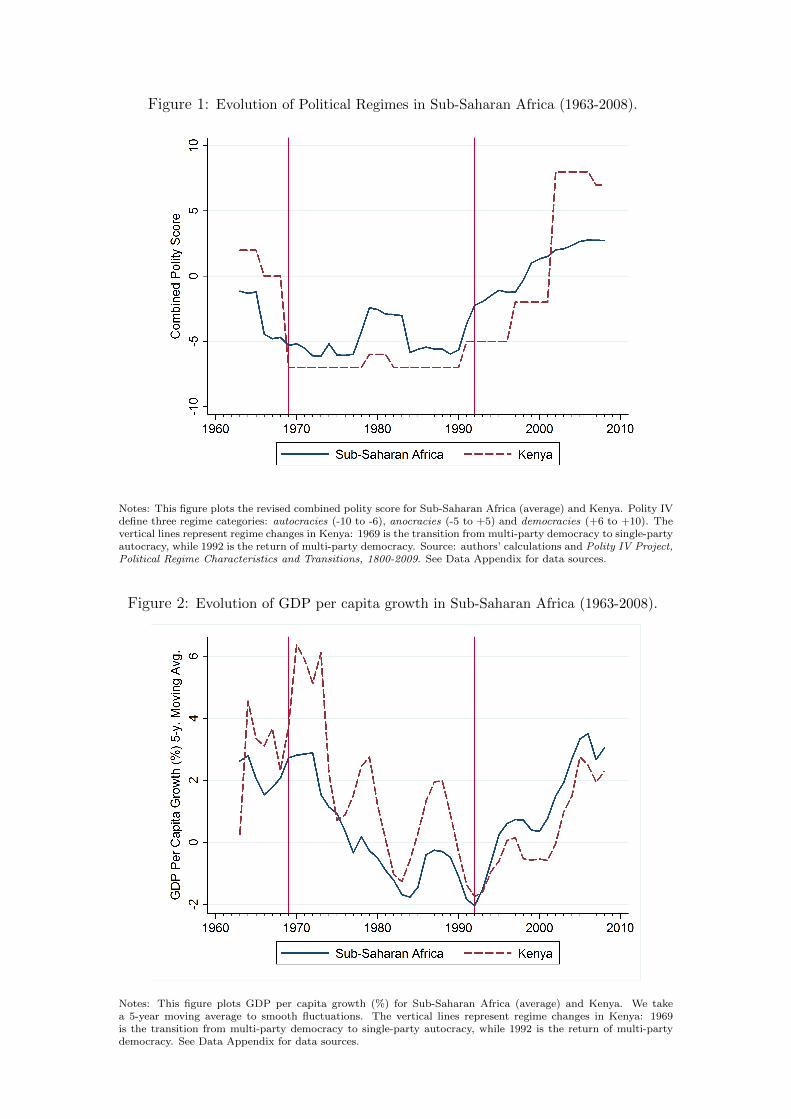
Figure 1: Evolution of Political Regimes in Sub-Saharan Africa (1963-2008).

Notes: This figure plots the revised combined polity score for Sub-Saharan Africa (average) and Kenya. Polity IVdefine three regime categories: autocracies (-10 to -6), anocracies (-5 to +5) and democracies (+6 to +10). Thevertical lines represent regime changes in Kenya: 1969 is the transition from multi-party democracy to single-partyautocracy, while 1992 is the return of multi-party democracy. Source: authors’ calculations and Polity IV Project,Political Regime Characteristics and Transitions, 1800-2009. See Data Appendix for data sources.

Figure 2: Evolution of GDP per capita growth in Sub-Saharan Africa (1963-2008).

Notes: This figure plots GDP per capita growth (%) for Sub-Saharan Africa (average) and Kenya. We takea 5-year moving average to smooth fluctuations. The vertical lines represent regime changes in Kenya: 1969is the transition from multi-party democracy to single-party autocracy, while 1992 is the return of multi-partydemocracy. See Data Appendix for data sources.

Figure

3:Evolution

ofKenya’sRoadNetworkforSelectedYears(1890-2002)

(i)

Paved

(ThickBlack),Im

proved(B

lack)an

dDirt(G

rey)Roads,an

dKikuyu(G

rey)an

dKalenjin(LightGrey)Areas.

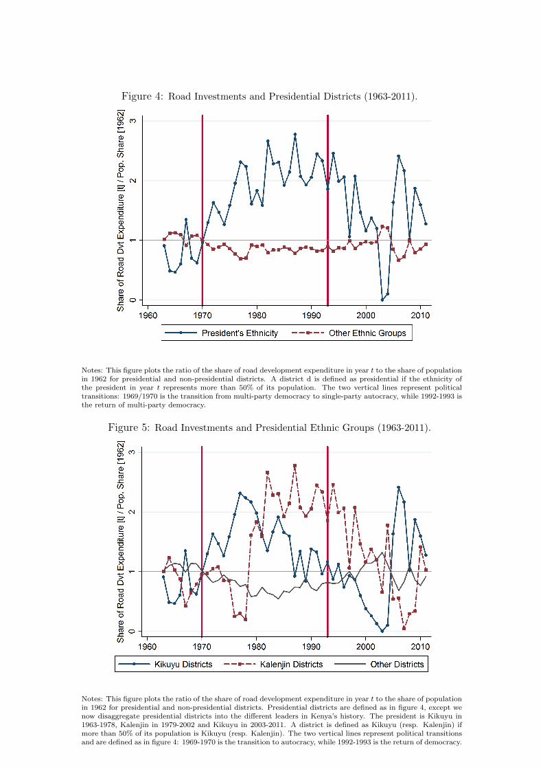
Figure 4: Road Investments and Presidential Districts (1963-2011).

Notes: This figure plots the ratio of the share of road development expenditure in year t to the share of populationin 1962 for presidential and non-presidential districts. A district d is defined as presidential if the ethnicity ofthe president in year t represents more than 50% of its population. The two vertical lines represent politicaltransitions: 1969/1970 is the transition from multi-party democracy to single-party autocracy, while 1992-1993 isthe return of multi-party democracy.

Figure 5: Road Investments and Presidential Ethnic Groups (1963-2011).

Notes: This figure plots the ratio of the share of road development expenditure in year t to the share of populationin 1962 for presidential and non-presidential districts. Presidential districts are defined as in figure 4, except wenow disaggregate presidential districts into the different leaders in Kenya’s history. The president is Kikuyu in1963-1978, Kalenjin in 1979-2002 and Kikuyu in 2003-2011. A district is defined as Kikuyu (resp. Kalenjin) ifmore than 50% of its population is Kikuyu (resp. Kalenjin). The two vertical lines represent political transitionsand are defined as in figure 4: 1969-1970 is the transition to autocracy, while 1992-1993 is the return of democracy.

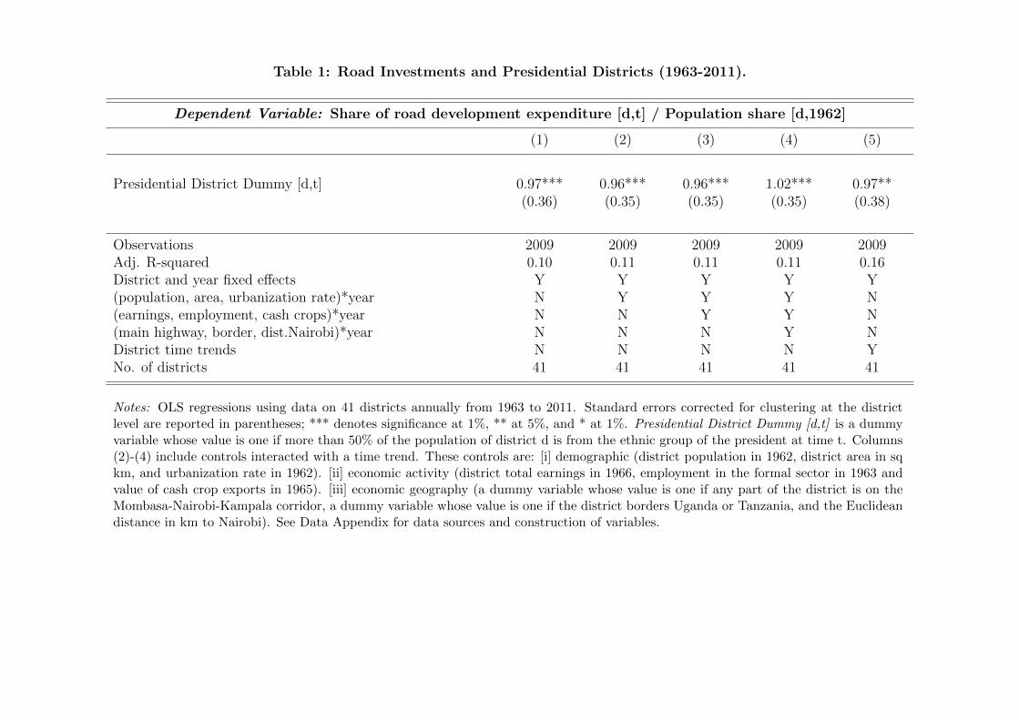
Table 1: Road Investments and Presidential Districts (1963-2011).

Dependent Variable: Share of road development expenditure [d,t] / Population share [d,1962]

(1) (2) (3) (4) (5)

Presidential District Dummy [d,t] 0.97*** 0.96*** 0.96*** 1.02*** 0.97**(0.36) (0.35) (0.35) (0.35) (0.38)

Observations 2009 2009 2009 2009 2009Adj. R-squared 0.10 0.11 0.11 0.11 0.16District and year fixed effects Y Y Y Y Y(population, area, urbanization rate)*year N Y Y Y N(earnings, employment, cash crops)*year N N Y Y N(main highway, border, dist.Nairobi)*year N N N Y NDistrict time trends N N N N YNo. of districts 41 41 41 41 41

Notes: OLS regressions using data on 41 districts annually from 1963 to 2011. Standard errors corrected for clustering at the districtlevel are reported in parentheses; *** denotes significance at 1%, ** at 5%, and * at 1%. Presidential District Dummy [d,t] is a dummyvariable whose value is one if more than 50% of the population of district d is from the ethnic group of the president at time t. Columns(2)-(4) include controls interacted with a time trend. These controls are: [i] demographic (district population in 1962, district area in sqkm, and urbanization rate in 1962). [ii] economic activity (district total earnings in 1966, employment in the formal sector in 1963 andvalue of cash crop exports in 1965). [iii] economic geography (a dummy variable whose value is one if any part of the district is on theMombasa-Nairobi-Kampala corridor, a dummy variable whose value is one if the district borders Uganda or Tanzania, and the Euclideandistance in km to Nairobi). See Data Appendix for data sources and construction of variables.

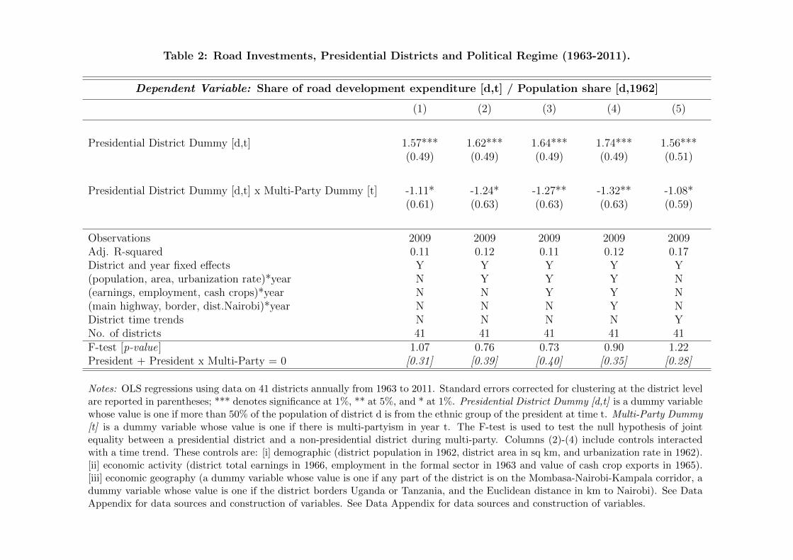
Table 2: Road Investments, Presidential Districts and Political Regime (1963-2011).

Dependent Variable: Share of road development expenditure [d,t] / Population share [d,1962]

(1) (2) (3) (4) (5)

Presidential District Dummy [d,t] 1.57*** 1.62*** 1.64*** 1.74*** 1.56***(0.49) (0.49) (0.49) (0.49) (0.51)

Presidential District Dummy [d,t] x Multi-Party Dummy [t] -1.11* -1.24* -1.27** -1.32** -1.08*(0.61) (0.63) (0.63) (0.63) (0.59)

Observations 2009 2009 2009 2009 2009Adj. R-squared 0.11 0.12 0.11 0.12 0.17District and year fixed effects Y Y Y Y Y(population, area, urbanization rate)*year N Y Y Y N(earnings, employment, cash crops)*year N N Y Y N(main highway, border, dist.Nairobi)*year N N N Y NDistrict time trends N N N N YNo. of districts 41 41 41 41 41F-test [p-value] 1.07 0.76 0.73 0.90 1.22President + President x Multi-Party = 0 [0.31] [0.39] [0.40] [0.35] [0.28]

Notes: OLS regressions using data on 41 districts annually from 1963 to 2011. Standard errors corrected for clustering at the district levelare reported in parentheses; *** denotes significance at 1%, ** at 5%, and * at 1%. Presidential District Dummy [d,t] is a dummy variablewhose value is one if more than 50% of the population of district d is from the ethnic group of the president at time t. Multi-Party Dummy[t] is a dummy variable whose value is one if there is multi-partyism in year t. The F-test is used to test the null hypothesis of jointequality between a presidential district and a non-presidential district during multi-party. Columns (2)-(4) include controls interactedwith a time trend. These controls are: [i] demographic (district population in 1962, district area in sq km, and urbanization rate in 1962).[ii] economic activity (district total earnings in 1966, employment in the formal sector in 1963 and value of cash crop exports in 1965).[iii] economic geography (a dummy variable whose value is one if any part of the district is on the Mombasa-Nairobi-Kampala corridor, adummy variable whose value is one if the district borders Uganda or Tanzania, and the Euclidean distance in km to Nairobi). See DataAppendix for data sources and construction of variables. See Data Appendix for data sources and construction of variables.

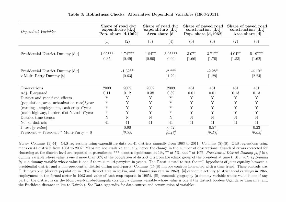
Table 3: Robustness Checks: Alternative Dependent Variables (1963-2011).

Share of road dvt Share of road dvt Share of paved road Share of paved road

Dependent Variable:expenditure [d,t]

Pop. share [d,1962]expenditure [d,t]Area share [d]

construction [d,t]Pop. share [d,1962]

construction [d,t]Area share [d]

(1) (2) (3) (4) (5) (6) (7) (8)

Presidential District Dummy [d,t] 1.02*** 1.74*** 1.84** 3.05*** 3.07* 3.71** 4.04** 5.19***[0.35] [0.49] [0.90] [0.99] [1.66] [1.70] [1.53] [1.62]

Presidential District Dummy [d,t] -1.32** -2.22* -2.28* -4.10*x Multi-Party Dummy [t] [0.63] [1.29] [1.29] [2.24]

Observations 2009 2009 2009 2009 451 451 451 451Adj. R-squared 0.11 0.12 0.38 0.39 0.01 0.01 0.13 0.13District and year fixed effects Y Y Y Y Y Y Y Y(population, area, urbanization rate)*year Y Y Y Y Y Y Y Y(earnings, employment, cash crops)*year Y Y Y Y Y Y Y Y(main highway, border, dist.Nairobi)*year Y Y Y Y Y Y Y YDistrict time trends N N N N N N N NNo. of districts 41 41 41 41 41 41 41 41F-test [p-value] 0.90 0.52 0.57 0.23President + President * Multi-Party = 0 [0.35] [0.48] [0.47] [0.63]

Notes: Columns (1)-(4): OLS regressions using expenditure data on 41 districts annually from 1963 to 2011. Columns (5)-(8): OLS regressions usingmaps on 41 districts from 1963 to 2002. Maps are not available annually, hence the change in the number of observations. Standard errors corrected forclustering at the district level are reported in parentheses; *** denotes significance at 1%, ** at 5%, and * at 10%. Presidential District Dummy [d,t] is adummy variable whose value is one if more than 50% of the population of district d is from the ethnic group of the president at time t. Multi-Party Dummy[t] is a dummy variable whose value is one if there is multi-partyism in year t. The F-test is used to test the null hypothesis of joint equality between apresidential district and a non-presidential district during multi-party. Columns (1)-(8) include controls interacted with a time trend. These controls are:[i] demographic (district population in 1962, district area in sq km, and urbanization rate in 1962). [ii] economic activity (district total earnings in 1966,employment in the formal sector in 1963 and value of cash crop exports in 1965). [iii] economic geography (a dummy variable whose value is one if anypart of the district is on the Mombasa-Nairobi-Kampala corridor, a dummy variable whose value is one if the district borders Uganda or Tanzania, andthe Euclidean distance in km to Nairobi). See Data Appendix for data sources and construction of variables.

Table

4:AdditionalRobustness

Check

s(1

963-2011).

Dep.V

ariable:Share

ofro

ad

developmentexpenditure

[d,t]/Population

share

[d,1962]

(1)

(2)

(3)

(4)

(5)

Pre

sid

enti

al

Dis

tric

tD

um

my

[d,t

]1.7

4***

2.1

0***

1.6

0***

2.3

4***

(0.4

9)

(0.7

7)

(0.5

0)

(0.5

8)

Pre

sid

enti

al

Dis

tric

tD

um

my

[d,t

]-1

.32**

-1.7

3*

-1.1

3-1

.45**

xM

ult

i-P

art

yD

um

my

[t]

(0.6

3)

(0.8

6)

(0.6

9)

(0.6

4)

Pre

sid

enti

al

Sh

are

[d,t

]2.3

0***

(0.5

6)

Pre

sid

enti

al

Sh

are

[d,t

]-1

.90***

xM

ult

i-P

art

yD

um

my

[t]

(0.6

6)

Pre

sid

enti

al

Dis

tric

tD

um

my

[d,t

]x

Wh

ite

Hig

hla

nd

s[d

]-0

.74

(0.9

0)

Pre

sid

enti

al

Dis

tric

tD

um

my

[d,t

]x

Wh

ite

Hig

hla

nd

s[d

]0.8

xM

ult

i-P

art

yD

um

my

[t]

(1.0

7)

Pre

sid

ent

Dis

tric

tof

Bir

th[d

,t]

0.9

(1.2

2)

Pre

sid

ent

Dis

tric

tof

Bir

th[d

,t]

-1.3

xM

ult

i-P

art

yD

um

my

[t]

(1.0

5)

Sec

on

dC

ab

inet

Gro

up

[d,t

]1.7

1***

(0.5

5)

Sec

on

dC

ab

inet

Gro

up

[d,t

]-1

.92**

xM

ult

i-P

art

yD

um

my

[t]

(0.8

2)

Ob

serv

ati

on

s2009

2009

2009

2009

2009

Ad

j.R

-squ

are

d0.1

20.1

20.1

20.1

20.1

3D

istr

ict

an

dye

ar

fixed

effec

tsY

YY

YY

(pop

ula

tion

,are

a,

urb

an

izati

on

rate

)*ye

ar

YY

YY

Y(e

arn

ings,

emp

loym

ent,

cash

crop

s)*yea

rY

YY

YY

(main

hig

hw

ay,

bord

er,

dis

t.N

air

ob

i)*ye

ar

YY

YY

YD

istr

ict

tim

etr

end

sN

NN

NN

No.

of

dis

tric

ts41

41

41

41

41

F-t

est

[p-value]

0.9

00.9

71.5

30.9

04.0

6*

Pre

sid

ent

+P

resi

den

t*

Mu

lti-

Part

y=

0[0.35]

[0.33]

[0.22]

[0.35]

[0.05]

Notes:

OL

Sre

gre

ssio

ns

usi

ng

data

on

41

dis

tric

tsan

nu

all

yfr

om

1963

to2011.

Sta

nd

ard

erro

rsco

rrec

ted

for

clu

ster

ing

at

the

dis

tric

tle

vel

are

rep

ort

edin

pare

nth

eses

;***

den

ote

ssi

gn

ifica

nce

at

1%

,**

at5%

,an

d*

at1%

.Presiden

tialDistrictDummy[d,t]

isa

du

mm

yva

riab

lew

hose

valu

eis

on

eif

more

than

50%

ofth

ep

opu

lati

onof

dis

tric

td

isfr

om

the

eth

nic

gro

up

of

the

pre

sid

ent

at

tim

et.

Multi-PartyDummy[t]

isa

du

mm

yva

riab

lew

hos

eva

lue

ison

eif

ther

eis

mu

lti-

part

yis

min

year

t.Presiden

tialShare

[d,t]

isth

ep

op

ula

tion

share

ofth

eet

hn

icgr

oup

ofth

ep

resi

den

tin

dis

tric

td

at

tim

et.

WhiteHighlands[d]

isa

dis

tric

td

um

my

equ

al

toon

eif

mor

eth

an50

%of

dis

tric

tare

aw

as

con

sid

ered

as

”W

hit

eH

igh

lan

ds”

du

rin

gco

lon

izati

on

.Presiden

tDistrictofBirth

[d,t]

isa

isa

du

mm

yva

riab

lew

hose

valu

eis

equ

al

toon

eif

dis

tric

td

isth

ep

resi

den

t’s

dis

tric

tof

bir

that

tim

et.

SecondCabinet

Group[d,t]

isa

du

mm

yva

riab

lew

hose

valu

eis

on

eif

more

than

50%

of

the

pop

ula

tion

of

the

dis

tric

tis

from

the

seco

nd

larg

est

eth

nic

gro

up

inth

eca

bin

etaft

erth

ep

resi

den

t’s

gro

up

at

tim

et.

Th

eF

-tes

tis

use

dto

test

the

nu

llhyp

oth

esis

of

join

teq

uali

tyb

etw

een

ap

resi

den

tial

dis

tric

tan

da

non

-pre

sid

enti

al

dis

tric

td

uri

ng

mu

lti-

par

ty.

Col

um

ns

(1)-

(5)

incl

ud

eco

ntr

ols

inte

ract

edw

ith

ati

me

tren

d.

Thes

eco

ntr

ols

are

the

sam

eas

inta

ble

s(1

)-(3

).S

eeD

ata

Ap

pen

dix

for

data

sou

rces

an

dco

nst

ruct

ion

of

vari

able

s.

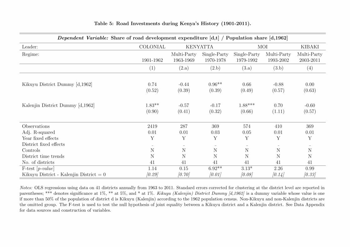
Table 5: Road Investments during Kenya’s History (1901-2011).

Dependent Variable: Share of road development expenditure [d,t] / Population share [d,1962]

Leader: COLONIAL KENYATTA MOI KIBAKI

Regime: Multi-Party Single-Party Single-Party Multi-Party Multi-Party1901-1962 1963-1969 1970-1978 1979-1992 1993-2002 2003-2011

(1) (2.a) (2.b) (3.a) (3.b) (4)

Kikuyu District Dummy [d,1962] 0.74 -0.44 0.96** 0.66 -0.88 0.00(0.52) (0.39) (0.39) (0.49) (0.57) (0.63)

Kalenjin District Dummy [d,1962] 1.83** -0.57 -0.17 1.88*** 0.70 -0.60(0.90) (0.41) (0.32) (0.66) (1.11) (0.57)

Observations 2419 287 369 574 410 369Adj. R-squared 0.01 0.01 0.03 0.05 0.01 0.01Year fixed effects Y Y Y Y Y YDistrict fixed effectsControls N N N N N NDistrict time trends N N N N N NNo. of districts 41 41 41 41 41 41F-test [p-value] 1.14 0.15 6.92** 3.13* 2.26 0.99Kikuyu District - Kalenjin District = 0 [0.29] [0.70] [0.01] [0.08] [0.14] [0.33]

Notes: OLS regressions using data on 41 districts annually from 1963 to 2011. Standard errors corrected for clustering at the district level are reported inparentheses; *** denotes significance at 1%, ** at 5%, and * at 1%. Kikuyu (Kalenjin) District Dummy [d,1962] is a dummy variable whose value is oneif more than 50% of the population of district d is Kikuyu (Kalenjin) according to the 1962 population census. Non-Kikuyu and non-Kalenjin districts arethe omitted group. The F-test is used to test the null hypothesis of joint equality between a Kikuyu district and a Kalenjin district. See Data Appendixfor data sources and construction of variables.

Appendices

A Data Appendix

The data used in this paper comes from a wide variety of sources. Summary statisticsfor the variables we construct are reported in Appendix A Table 1.

Spatial Units:The data we assemble cover the 41 districts of Kenya, for the period 1889 to 2011. Wefix district boundaries according to the administrative map at independence, in 1963,and follow these units across the period 1963-2011.1 Kenya is administratively dividedinto provinces, districts, location and sub-locations.

Road Expenditure Data:We assemble a road development expenditure dataset for 41 districts, annually from 1901to 2011. In general, road expenditure data can be disaggregated into development expen-diture (which are new investments) and recurrent expenditures (primarily maintenance).The Kenyan administrative records only allow to track road development expenditure atthe district level. Unfortunately, recurrent road expenditure, though reported annually,is only available at the national level. To construct this database of road investments,we use various annual reports which exhaustively list individual road projects (e.g., fromtown A to town B through town C) and their related costs.2 When a road project spansmore than one district, we use GIS to understand the layout of the affected road andhow many kilometers are affected within each district. We then decompose expenditureacross the affected districts assuming an equal distribution of costs along the total lengthof this layout.3 This exercise allows us to have a panel data set of road expenditure for

1District boundaries were subsequently redrawn after 1992. However, these could be drivenby political motives, e.g. gerry-meandering.

2The reports we use for the pre-independence period are: Annual Colonial Reports of theKenya Colony 1897-1930, Blue Books of the Kenya Colony 1912-1916, 1926-1938 and 1945-1946, Public Works Department Reports of the Kenya Colony 1913, 1923, 1926-1938, 1945-1956,Financial Reports of the Kenya Colony 1922-1960, Development and Reconstruction Reports ofthe Kenya Colony 1946-1952, Road Authority Reports of the Kenya Colony 1949-1962, NativeAffairs Reports of the Kenya Colony 1924-1947. The reports we use for the post-independenceperiod are: Development Estimates of Kenya 1963-2011, Physical Infrastructure Sector MTEFReport of Kenya 2007/2008-2009/2010 and 2009/2010-2011/2012. We then use DevelopmentEstimates of Kenya 1963-2011 and Recurrent Estimates of Kenya 1963-2011 to compare theannual aggregate amounts spent on road investments to: (i) the total investment budget, (ii)investments in other public goods (education, health and water development), and (iii) the roadmaintenance budget. We also estimate the share of road expenditure provided by foreign aid.

3The information soon after independence, for the period 1963-1973, is recorded as expen-diture on road programs, which are collections of individual road projects. We use varioussupplementary documents to understand how the total cost of these road programs could be

41 districts annually from 1901 to 2001.4 We have 41 districts and 111 years, hence 4551observations.

Road Building Data:We create a district road building data by putting together a novel GIS database of theKenyan road network, at regular intervals for the period 1889 to 2002.5 To constructthe GIS database, we initially start with a GIS database containing contemporary roadsfrom Global GIS. We then use various sets of historical maps and reports to recreatethe evolution of the GIS network backwards in time.6 For the period 1889 to 2002, weare able to distinguish between two categories of road type - paved and unpaved roads.For the more recent period 1955-2002, we are also able to distinguish a further type ofroad - improved (laterite) roads.7 No updated road map of Kenya exists post-2002. Thelast Government of Kenya map was completed in 2002, and no commercial road mapshave been updated after that year.8 Using GIS tools, we then superpose our districtboundaries on the road network and create a district-year panel data set of the totallength (km) of paved roads, improved and dirt roads.

Cabinet Data:We construct a panel data set of all the cabinet members for all the election years inthe period 1963 to 2011. There are 13 such cabinet appointments. We assemble several

disaggregated between individual road projects and then mapped onto the GIS database foranalysis at the district level. These documents are the 5-year Development Plan of Kenya 1964-1970, 1966-1970, 1970-1974 and 1974-1978, and a series of Road Program Operational Reportsdirectly available on the website of the World Bank: http://www.worldbank.org/projects. Dur-ing the initial years, most of the road programs were funded by the World Bank, we obtained foreach project an Operational Report which details out each road program and the cost for eachindividual road project.

4Road expenditure is reported in British Pounds before 1920, East African Pounds for theperiod 1921-1966, Kenyan Pounds for the period 1967-1999, and Kenya Shillings for the period2000 onwards. Using Officer (2009) and IMF (2011), we convert these amounts to current US$and use a deflator series of the US$ to obtain those amounts in constant 2000$.

5We have annual data for the period 1889-1961, and for the following years - 1964, 1967, 1969,1972, 1974, 1979, 1981, 1987, 1989, 1992 and 2002.

6The maps we use are: Map for the Colony of Kenya 1959, Michelin National Map for Centraland South Africa 1961, 1964, 1967, 1969, 1972, 1974, 1979, 1981, 1984, 1987, 1989 and 1992, andSurvey of Kenya Map 1948, 1955, 1967, 1972, 1991 and 2002. The reports we use are as listedin footnote 2. We check our methodology by comparing the evolution of the network providedby Soja (1968).

7Note there were no paved roads in Kenya prior to 1945. The colonial reports do not distin-guish between improved and dirt roads before 1955. Michelin maps for the period 1961-1992 areconsistent across time and display the quality of each road using a consistent classification. Wecross-check the Michelin maps with the Government of Kenya maps (known as Survey of KenyaMaps). Lastly, we use the 2002 Survey of Kenya Map to recreate the paved, improved and dirtnetwork in 2002.

8A discussion with various road mapping agencies, e.g. Michelin, confirmed that most Africancountries have stopped providing road mapping information from the early-1990s.

characteristics of the cabinet members - their ministerial portfolio, ethnicity and districtof birth. This dataset allows us to track the evolution of each ethnic group’s represen-tation in the politics of Kenya. We use various data sources to construct the cabinetpanel database. 9 We then learn the district of birth for each cabinet member fromrecords kept at the Kenyan Parliamentary Library. Finally, the ethnicity of prominentcabinet members is well-known, while the information for the less prominent politiciansis obtained in several ways. We use third-party sources: (i) the Weekly Review magazinein the Moi period would often list out the cabinet and ethnicity of cabinet members,(ii) we cross checked our findings with Hornsby (1985), Ahluwalia (1996) and Hornsby(2010), and (iii) the direct help of several journalists from top dailies in Kenya.10 Theconstruction of this database allows us to calculate the share of each ethnic group in thecabinet. Appendix A Table 2 tabulates the ethnic shares across the different cabinetyears. The Development Estimates of Kenya allows us to rank annually the differentministerial portfolios in terms of their budgets. We calculate other cabinet share mea-sures: (i) for each ethnic group we use the president and the top ten fiscal positions,and (ii) we create from the same source the listing of cabinet appointments (president,vice-president/prime minister, minister of finance, minister of defence, etc.). We thenrecalculate cabinet shares for each ethnic group using the president and the top tenhierarchical positions according to the list presented.11

Ethnic Census Data:We use the 1962 population census of Kenya to obtain our ethnic composition of dis-tricts. The 1962 ethnic census is tabulated at the location level (which is one level belowthe district).12 We use GIS to transform the 1962 ethnic data at the location level todistrict level data using the district boundaries (41) of 1963. We aggregate the 41 tribesinto an aggregated classification of 13 ethnic groups, which is standard when analyz-ing Kenyan politics: Kikuyu, Kalenjin, Kamba, Luo, Luhya, Maasai, Coastal, Embu,Kisii, Meru, Somali, Turkana-Samburu and Other (Other Africans, Arabs, Asians, Non-Africans). Appendix A Figure 1 displays the main ethnic groups for each location (168)in 1962 and district boundaries (41) at independence, in 1963. This confirms that dis-trict boundaries were created to isolate ethnic groups. We tabulate the ethnic profile ofKenya’s population across all the census years (1948, 1962, 1969, 1979, 1989 and 2009).13

Appendix A Table 3 reports the national ethnic shares, and reveals the stability of ethnicgroups across time.

9We use the following publications: The National Assembly: List of Members, Organizationof the Government of Kenya, and Encyclopedia of Sub-Sahara Africa: Kenya.

10We are grateful to Charles Hornsby for his assistance at various stages and to Ann Mbuguafor her help in Kenya.

11Tables not shown but available upon request.12There are 168 locations.13Unfortunately, ethnic data from the 1999 census was never made public. Instead, we use

as a proxy the ethnic distribution available in the report of the nationally representative 2003Kenya Demographic and Health Survey.

Political Economy:Presidential District Dummy [d,t] is a dummy variable whose value is one if more than50% of the district d population is from the ethnic group of the president in year t.The ethnic group of the president is Kikuyu (Kenyatta) in 1963-1978, Kalenjin (Moi) in1979-2002 and Kikuyu (Kibaki) again in 2003-2011. Multi-Party Dummy [t] is dummyvariable whose value is one if there is a multi-party democracy in year t. The multi-partyyears in Kenya were 1963-1969 and 1993-2011 in our sample. 14 Kikuyu District Dummy[d] (resp. Kalenjin District Dummy [d]) is a dummy variable whose value is one if morethan 50% of the population of district d is Kikuyu (resp. Kalenjin). Presidential Share[d,t] is the share of the president’s ethnic group in district d at time t. White Highlands[d] is a dummy equal to one if more than 50% of district area was considered as ”WhiteHighlands”. The White Highlands was a demarcated area set aside by the Kenya Colonyfor White settlers.15 President District of Birth [d,t] is a dummy equal to one is districtd is the president’s district of birth at time t. 16. Second Cabinet Group [d,t] is a dummyequal to one if more than 50% of the population of the district is from the second largestethnic group in the cabinet after the president’s group at time t.17 There is no clearcoalition member in the period 1970-1978 (7 ethnic groups share the second position inthis period) and there are two ethnic groups in the period 1993-1997.18 Lastly, we createRoad Minister District of Birth [d,t], a dummy variable whose value is one if district dis the district of birth of the road minister.19

Control Variables:We use various documents to reconstruct a set of socioeconomic and demographic vari-

14Expenditure data is budgeted for year t, which runs from June [t−1] to June [t]. As a result,Moi’s impact has to be considered from 1979 (June 1978-June 1979) and Kibaki’s impact from2003 (June 2002-June 2003). Similarly, the transition to autocracy in November 1969 is effectivefrom 1970 (June 1969-June 1970) and the transition to democracy in December 1992 is effectivefrom 1993 (June 1992-June 1993). We adapt the political economy variables to reflect this whenwe use paved road construction as an outcome to ensure we are consistent.

15We digitize a 1958 land classification map from the Survey of Kenya to create this dummy.16Kenyatta (for the period 1963-1978) was born in Kiambu district, Moi (for the period 1979-

2002) was born in Baringo district, and Kibaki (for the period 2003-2011) was born in Nyeridistrict.

17The second cabinet ethnic group are the Luos for the period 1963-1969, the Kikuyus for theperiod 1979-2002, the Kambas for the period 1993-1997 and the Luhyas for the period 1993 to2011.

18We obtain a rather similar ethnic chronology of the second group when considering the topfiscal positions, the top hierarchical positions or the ethnicity of the vice-president. Besides,there are no years for which the second group is not identified using those alternative definitions.We construct alternative measures of the second cabinet group based on those three differentdefinitions: Vice-Presidential District Dummy [d,t], Second Cabinet Group [d,t] Fiscal and Sec-ond Cabinet Group [d,t] Hierarchical. We also create Cabinet Share of Maj. Ethnic Group [d,t]which is the cabinet share at time t of the majoritarian ethnic group in district d.

19We use different measures of having access to the road ministry, by also looking at theethnicity of the road minister, and the district of birth and ethnicity of the public works minister.

ables at the district level. We obtain district population and urbanization rates fromthe reports of the decadal Population and Housing Censuses of Kenya (1962, 1969,1979, 1989 and 1999). District area (sq km) is estimated using GIS tools on the basisof 1963 administrative boundaries. We use the annual Statistical Abstracts of Kenyato reconstruct total district employment and total district earnings (in 2000$) in theformal sector.20 The former variable is available annually from 1963 to 2006, while thelatter variable is available annually from 1966 to 2006. The Development Plan of Kenya1964-1970 reports cash crop production (coffee, tea and sisal) at the district level for theyear 1964-1965. We then use the 1965 export price in 2000$ (FAO 2011) to calculate thedistrict total value of cash crop exports in 1965.21 We use GIS to create: (i) a dummyvariable whose value is one if any part of the district is on the Mombasa-Nairobi-Kampalacorridor, (ii) a dummy variable whose value is one if the district borders Uganda or Tan-zania, (iii) a variable capturing the Euclidian distance (in km) of each district centroidto Nairobi. We use a digitized land classification map to estimate the share of districtarea that was part of the former White Highlands. Appendix A Figure 2 displays themain road network at independence and the White Highlands. It confirms that most ofthe colonial road network was located in the White Highlands.

Macroeconomic and Democracy Data:Data on political regimes in Sub-Saharan African countries and Kenya is obtained fromthe Polity IV Project, a well-known database on political regime characteristics and tran-sitions. We use the ”Combined Polity Score” which ranges in value from -10 (hereditarymonarchy) to +10 (consolidated democracy). Polity IV recommends to follow this clas-sification: autocracies (-10 to -6), anocracies (-5 to +5) and democracies (+6 to +10).The average combined policy score for Sub-Saharan Africa is calculated using individualpolity scores and the population of each country as weights (obtained from WB (2011)).We also use WB (2011) to get data on GDP per capita growth in Sub-Saharan Africaand Kenya.

20The data is reported in Kenyan Shillings. Using Officer (2009) and IMF (2011), we convertthose amounts to current US$ and deflate them to get constant 2000$.

21We use this data to identify the cash crop specialization of each presidential group. Data ondistortions to agricultural incentives for each crop-year is obtained from Anderson and Valenzuela(2008).

References

Ahluwalia, P. (1996): “Post Colonialism and the Politics of Kenya,” New York: NovaScience.

Anderson, K., and E. Valenzuela (2008): Estimates of Global Distortions to Agri-cultural Incentives, 1955 to 2007. Washington DC: World Bank.

FAO (2011): FAOSTAT. Rome: Food and Agricultural Organization.

Hornsby, C. (1985): “The Member of Parliament in Kenya, 1969-1983: the Election,Background and Position of the Representative and the Implications for his Role inthe One-Party State,” Unpublished thesis, Oxford University.

(2010): “Database of Kenyan Members of Parliament,” Unpublished, PersonalCommunication.

IMF (2011): International Financial Statistics. Washington D.C.: International Mone-tary Fund.

Officer, L. (2009): Exchange Rates Between the United States Dollar and Forty-oneCurrencies. MeasuringWorth Project.

Soja, E. (1968): “The Geography of Modernization in Kenya; a Spatial Analysis ofSocial, Economic, and Political Change,” Syracuse geographical series no. 2.

WB (2011): Word Development Indicators. Washington D.C.: World Bank.

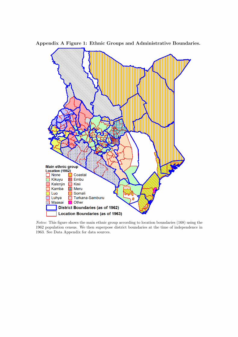
Appendix A Figure 1: Ethnic Groups and Administrative Boundaries.

Notes: This figure shows the main ethnic group according to location boundaries (168) using the1962 population census. We then superpose district boundaries at the time of independence in1963. See Data Appendix for data sources.

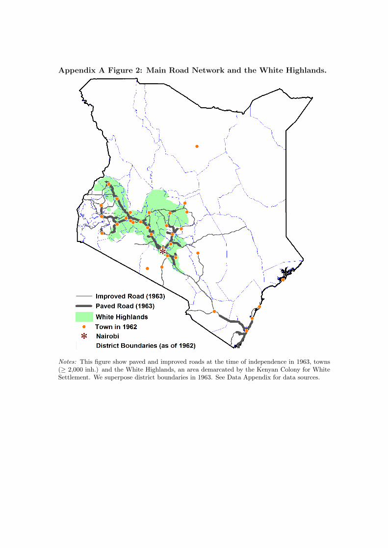
Appendix A Figure 2: Main Road Network and the White Highlands.

Notes: This figure show paved and improved roads at the time of independence in 1963, towns(≥ 2,000 inh.) and the White Highlands, an area demarcated by the Kenyan Colony for WhiteSettlement. We superpose district boundaries in 1963. See Data Appendix for data sources.

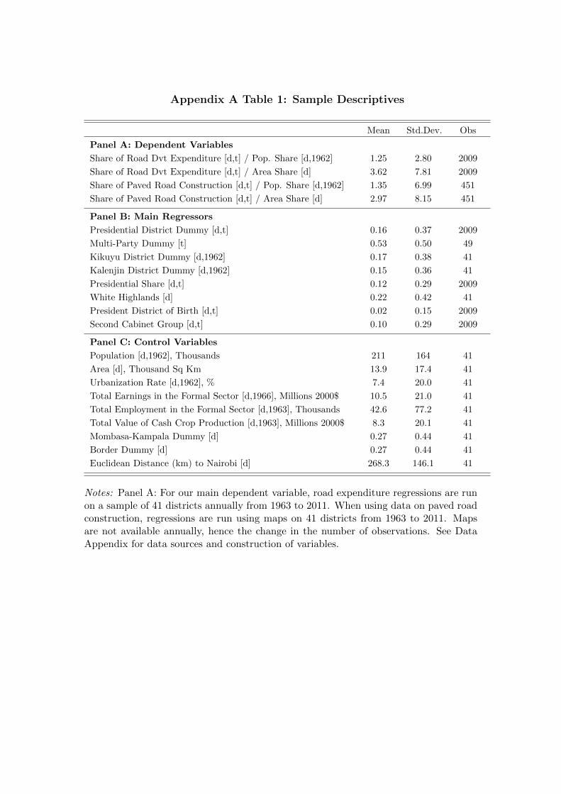
Appendix A Table 1: Sample Descriptives

Mean Std.Dev. Obs

Panel A: Dependent Variables

Share of Road Dvt Expenditure [d,t] / Pop. Share [d,1962] 1.25 2.80 2009

Share of Road Dvt Expenditure [d,t] / Area Share [d] 3.62 7.81 2009

Share of Paved Road Construction [d,t] / Pop. Share [d,1962] 1.35 6.99 451

Share of Paved Road Construction [d,t] / Area Share [d] 2.97 8.15 451

Panel B: Main Regressors

Presidential District Dummy [d,t] 0.16 0.37 2009

Multi-Party Dummy [t] 0.53 0.50 49

Kikuyu District Dummy [d,1962] 0.17 0.38 41

Kalenjin District Dummy [d,1962] 0.15 0.36 41

Presidential Share [d,t] 0.12 0.29 2009

White Highlands [d] 0.22 0.42 41

President District of Birth [d,t] 0.02 0.15 2009

Second Cabinet Group [d,t] 0.10 0.29 2009

Panel C: Control Variables

Population [d,1962], Thousands 211 164 41

Area [d], Thousand Sq Km 13.9 17.4 41

Urbanization Rate [d,1962], % 7.4 20.0 41

Total Earnings in the Formal Sector [d,1966], Millions 2000$ 10.5 21.0 41

Total Employment in the Formal Sector [d,1963], Thousands 42.6 77.2 41

Total Value of Cash Crop Production [d,1963], Millions 2000$ 8.3 20.1 41

Mombasa-Kampala Dummy [d] 0.27 0.44 41

Border Dummy [d] 0.27 0.44 41

Euclidean Distance (km) to Nairobi [d] 268.3 146.1 41

Notes: Panel A: For our main dependent variable, road expenditure regressions are runon a sample of 41 districts annually from 1963 to 2011. When using data on paved roadconstruction, regressions are run using maps on 41 districts from 1963 to 2011. Mapsare not available annually, hence the change in the number of observations. See DataAppendix for data sources and construction of variables.

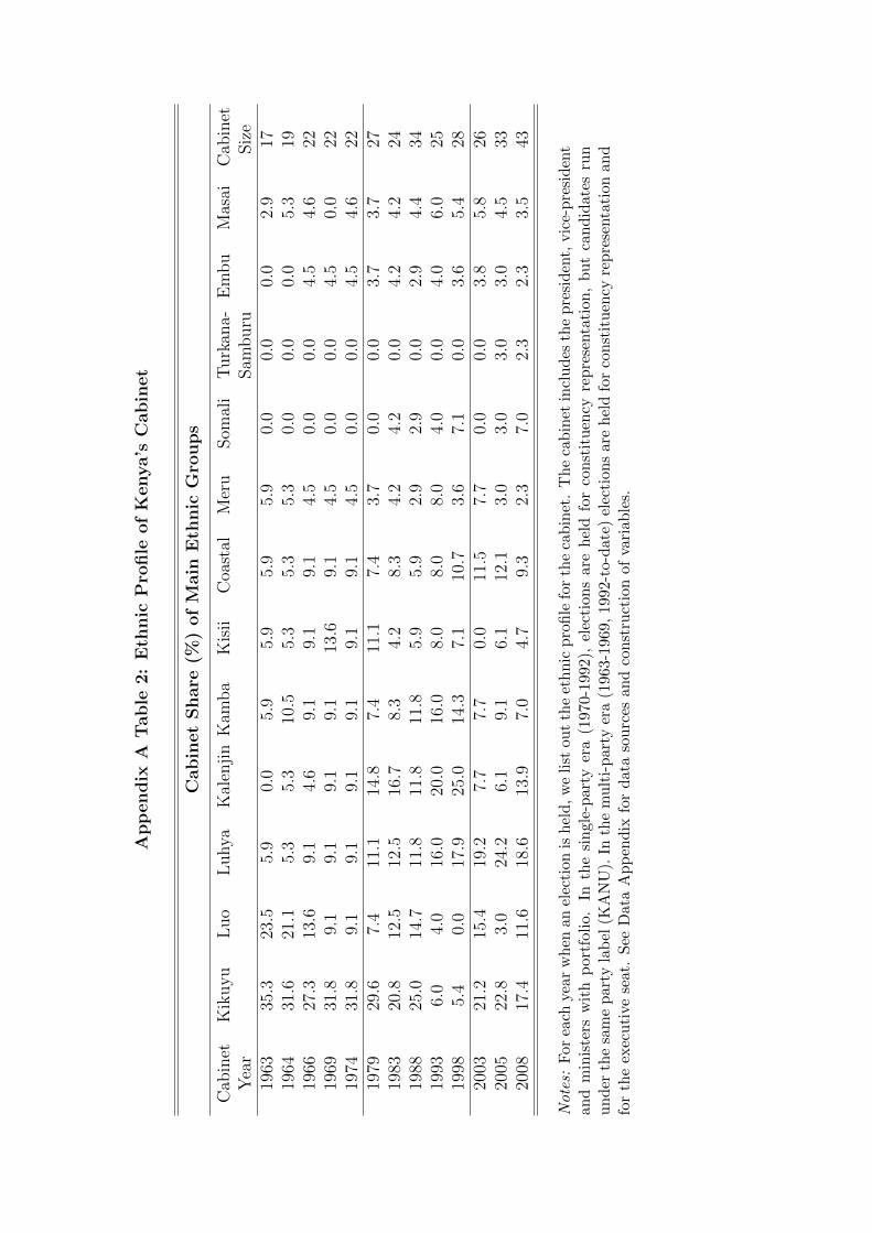
App

endix

AT

able

2:

Eth

nic

Pro

file

of

Kenya’s

Cab

inet

Cabin

et

Share

(%)

of

Main

Eth

nic

Gro

ups

Cab

inet

Year

Kikuyu

Luo

Luhya

Kalenjin

Kam

ba

Kisii

Coastal

Meru

Som

ali

Turkan

a-Sam

buru

Embu

Masai

Cab

inet

Size

1963

35.3

23.5

5.9

0.0

5.9

5.9

5.9

5.9

0.0

0.0

0.0

2.9

171964

31.6

21.1

5.3

5.3

10.5

5.3

5.3

5.3

0.0

0.0

0.0

5.3

191966

27.3

13.6

9.1

4.6

9.1

9.1

9.1

4.5

0.0

0.0

4.5

4.6

221969

31.8

9.1

9.1

9.1

9.1

13.6

9.1

4.5

0.0

0.0

4.5

0.0

221974

31.8

9.1

9.1

9.1

9.1

9.1

9.1

4.5

0.0

0.0

4.5

4.6

221979

29.6

7.4

11.1

14.8

7.4

11.1

7.4

3.7

0.0

0.0

3.7

3.7

271983

20.8

12.5

12.5

16.7

8.3

4.2

8.3

4.2

4.2

0.0

4.2

4.2

241988

25.0

14.7

11.8

11.8

11.8

5.9

5.9

2.9

2.9

0.0

2.9

4.4

341993

6.0

4.0

16.0

20.0

16.0

8.0

8.0

8.0

4.0

0.0

4.0

6.0

251998

5.4

0.0

17.9

25.0

14.3

7.1

10.7

3.6

7.1

0.0

3.6

5.4

282003

21.2

15.4

19.2

7.7

7.7

0.0

11.5

7.7

0.0

0.0

3.8

5.8

262005

22.8

3.0

24.2

6.1

9.1

6.1

12.1

3.0

3.0

3.0

3.0

4.5

332008

17.4

11.6

18.6

13.9

7.0

4.7

9.3

2.3

7.0

2.3

2.3

3.5

43

Note

s:F

orea

chye

ar

wh

enan

elec

tion

ish

eld

,w

eli

stou

tth

eet

hn

icpro

file

for

the

cab

inet

.T

he

cab

inet

incl

ud

esth

ep

resi

den

t,vic

e-p

resi

den

tan

dm

inis

ters

wit

hp

ort

foli

o.In

the

sin

gle

-part

yer

a(1

970-

1992

),el

ecti

ons

are

hel

dfo

rco

nst

itu

ency

rep

rese

nta

tion

,b

ut

can

did

ate

sru

nu

nd

erth

esa

me

par

tyla

bel

(KA

NU

).In

the

mu

lti-

part

yer

a(1

963-

1969

,19

92-t

o-d

ate)

elec

tion

sar

eh

eld

for

con

stit

uen

cyre

pre

senta

tion

an

dfo

rth

eex

ecu

tive

seat

.S

eeD

ata

Ap

pen

dix

for

data

sou

rces

and

con

stru

ctio

nof

vari

able

s.

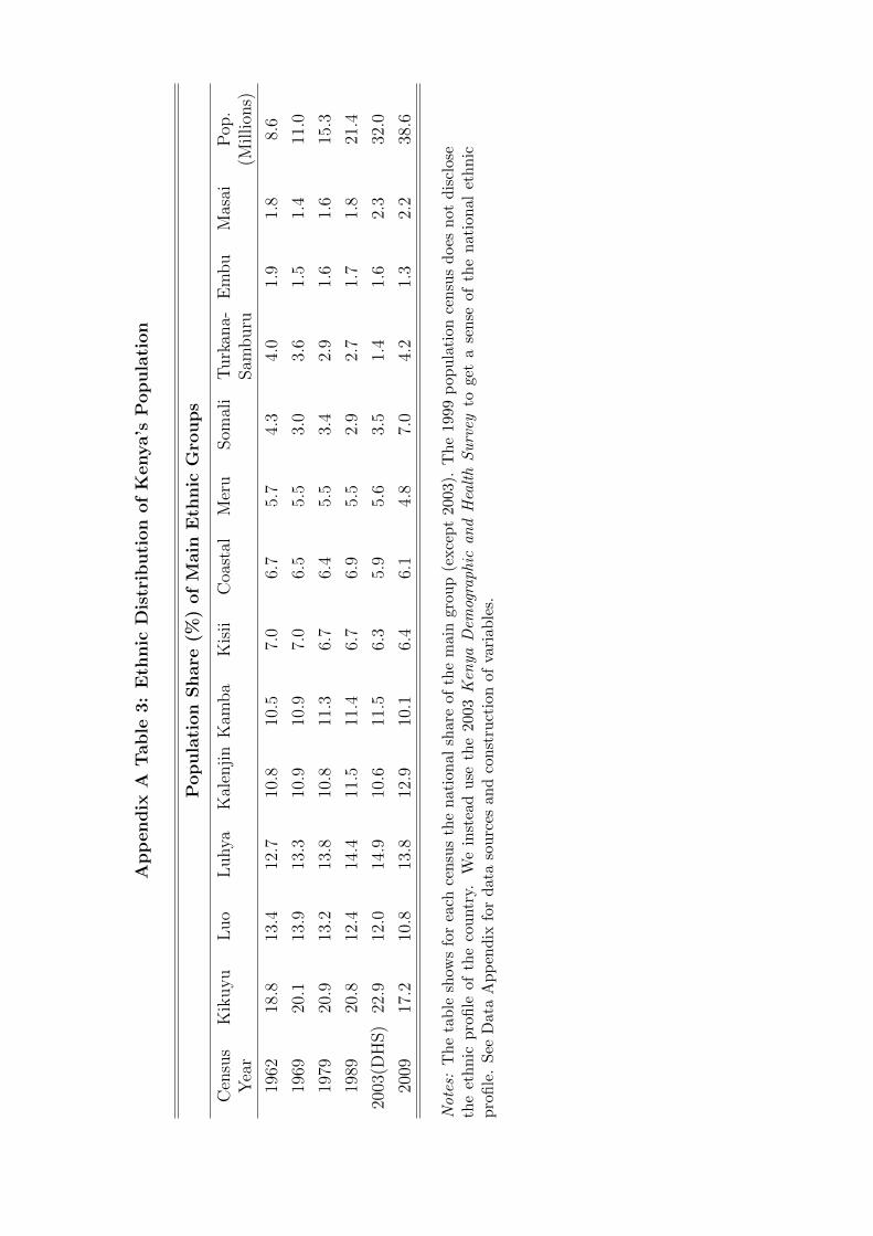
App

endix

AT

able

3:

Eth

nic

Dis

trib

uti

on

of

Kenya’s

Popu

lati

on

Popula

tion

Share

(%)

of

Main

Eth

nic

Gro

ups

Census

Year

Kikuyu

Luo

Luhya

Kalenjin

Kam

ba

Kisii

Coastal

Meru

Som

ali

Turkan

a-Sam

buru

Embu

Masai

Pop

.(M

illion

s)

1962

18.8

13.4

12.7

10.8

10.5

7.0

6.7

5.7

4.3

4.0

1.9

1.8

8.6

1969

20.1

13.9

13.3

10.9

10.9

7.0

6.5

5.5

3.0

3.6

1.5

1.4

11.0

1979

20.9

13.2

13.8

10.8

11.3

6.7

6.4

5.5

3.4

2.9

1.6

1.6

15.3

1989

20.8

12.4

14.4

11.5

11.4

6.7

6.9

5.5

2.9

2.7

1.7

1.8

21.4

2003(D

HS)

22.9

12.0

14.9

10.6

11.5

6.3

5.9

5.6

3.5

1.4

1.6

2.3

32.0

2009

17.2

10.8

13.8

12.9

10.1

6.4

6.1

4.8

7.0

4.2

1.3

2.2

38.6

Note

s:T

he

tab

lesh

ows

for

each

cen

sus

the

nati

onal

shar

eof

the

mai

ngr

oup

(exce

pt

2003

).T

he

1999

pop

ula

tion

cen

sus

does

not

dis

close

the

eth

nic

pro

file

of

the

cou

ntr

y.W

ein

stea

du

seth

e20

03K

enya

Dem

ogra

phic

an

dH

ealt

hS

urv

eyto

get

ase

nse

of

the

nati

on

al

eth

nic

pro

file

.S

eeD

ata

Ap

pen

dix

for

dat

aso

urc

esan

dco

nst

ruct

ion

ofva

riab

les.

B Mathematical Proof

Algebra: is ηBA decreasing in θ?

ηBA =ηAA

θ

R′(ηAA)− π − 1− π

θ= 0

∂ηAA

∂θ= −

1−π2θ

12

R′′(ηAA)> 0

dηBA

dθ=

∂ηAA

∂θ

1

θ− ηAA

2θ12

= −1−π2θ

12

R′′(ηAA)

1

θ− ηAA

2θ12

1

2θ12

[1− π

−θR′′(ηAA)− ηAA

]1

2θ12

[R′(ηAA)− π

−R′′(ηAA)− ηAA

]1

2θ12

[R′(ηAA)− π + ηAAR′′(ηAA)

−R′′(ηAA)

]So for monotonically decreasing we need

R′(ηAA)− π + ηAAR′′(ηAA) < 0

which will not be true for R almost linear.

C Additional Results

This appendix provides additional results that are discussed in the text.

C.1 Robustness checks

C.1.1 Improved Road Construction

In column (6) of Table 3, we find that presidential districts obtain 4.71 times more pavedroads than their population share. We also find that during democratic years this effectis significantly dampened. Note that paved roads are either improved or earthen roadsthat have been upgraded, or are newly constructed roads which are paved. When usingas a dependent variable the ratio of the share of improved road construction in districtd at time t to the population share of district d in 1962, we find no statistical differ-ence between presidential and non-presidential districts, whether the political period isdemocracy or autocracy. The coefficient of the presidential district dummy is equal to0.25 and is non-significant, while the coefficient on its interaction with the multi-partydummy is -0.25 and non-significant. This suggests that the president only favors hisown ethnic group by granting them more paved roads. Other ethnic groups are notcompensated by receiving more improved roads.1

C.1.2 Non-Linearity in Time Trends for Control Variables

The effect of control variables could be non-linear over time. For instance, it could berational to build roads around the capital Nairobi first, and later extend road buildingto the rest of the country. The negative effect of distance to Nairobi would decreaseover time and we would fail to capture this by interacting it with a linear trend. Thiscould explain why Kikuyu areas (which are close to Nairobi) obtain roads first, andwhy Kalenjin areas (which are further away from Nairobi) later obtain roads. Likewise,the government could build roads in already developed areas first and then expand thenetwork to remote/poor areas. This could explain why Kikuyu areas (which export morecash crops and have more formal employment at independence) receive more roads first,and why Kalenjin areas later obtain roads. We run our baseline regression (see AppendixC Table 1, column (1)), and interact the control variables with a time trend and timetrend square. The interaction of the presidential district and multi-party dummies areinsignificant at the standard levels (see column (2)), but the point estimates are similar.

C.1.3 Regression To The Mean

Regression to the mean could account for our findings. Kikuyu (until 1979) and Kalenjin(until 1992) districts have received large shares of road investments. The fact that in-vestments shifted to Kalenjin districts after 1979 and to other districts after 1992 could

1Results not shown but available upon request.

be explained by low economic and social returns of new road investments in those par-ticular districts. However, this is not warranted given network effects, as the economicreturns of new road investments might not be decreasing in past investments. Second,even if a district is spatially congested, the president can upgrade the network (bitum-enization, increasing the number of lanes, etc.). Lastly, we can control for the numberof years a district has been a presidential district. Coefficients are unaltered, althoughless precisely estimated (see Appendix C Table 1, column (3)).

C.1.4 Spatial Dependence

If observations are spatially correlated, estimated standard errors are incorrect. Forinstance, if neighboring observations are positively correlated, estimated standard errorswould be too low, causing incorrect inference. The cluster covariance matrix (CCE)approach is to cluster observations so that group-level averages are independent.2 Asdemonstrated in Bester, Conley, and Hansen (2011), clustering observations using fewgroups can ensure spatial independence. We subject our main results to various differentlevels of clustering. First, we cluster observations at the ethnic group level (13 groups)and province level (8 groups). Second, we use district geographical coordinates andaverage longitude and latitude for Kenya to separate districts into four quadrants: North-West, North-East, South-West and South-East. We cluster observations at the quadrantlevel (4 groups). Third, we cluster the data using North vs. South (2 groups) or Westvs. East (2 groups). We only report results for standard errors clustered at the ethnicgroup level (see Appendix C Table 1, column (4)) and at the province level (column(5)), our results are robust to these forms of clustering. The plug-in HAC covariancematrix approach is to plug-in a covariance matrix estimator that is consistent underheteroskedasticity and autocorrelation of unknown form. This approach models spatialdependence instead of time dependence, and has been popularized by Conley (1999). Itcan be tested in STATA by specifying that each observation is related to any observationless thanX km away.3 We use the geographical coordinates of each district to test variousthresholds: 100 km, 200 km or more than 200 km. We only report results with the 200km threshold (see column (6)) but other results are available upon request. Resultsremain unchanged after accounting for spatial dependence.

C.1.5 Tax Discrimination

It could be that our results are not related to ethnic favoritism at all, and instead thepresidential ethnic group receives more transfers because it also pays more taxes. Wetest this hypothesis by investigating whether the president taxes differently the crop inwhich her own group specializes. Using production data at the district level in 1965for coffee and tea, the two main exports of Kenya, we observe that coffee is primarily a

2We thank Timothy Conley for pointing this very simple method to us.3We thank Jordan Rappaport for sharing his STATA code ”gls sptl.005.do”.

Kikuyu crop while tea is primarily a Kalenjin crop.4 We test if the president, whetherKikuyu or Kalenjin, taxes more (or less) her own ethnic group than the other ethnicgroup, in democracy versus autocracy. For both coffee and tea, we know the yearlytaxation rate from 1963 to 2004.5 The rate is negative when the producer price decidedby the government is lower than the international export price, which is interpreted astaxation. Conversely, the rate is positive when the producer price is higher than theexport price, which is interpreted as a subsidy. The average taxation rate for the period1963-2004 was -0.107, this implies that 10.7% of the output value of coffee and tea wascaptured by the government. We regress the yearly taxation rate on a dummy if it is thecrop of the president (coffee when Kikuyu, tea when Kalenjin) and its interaction withthe multi-party dummy, including time and crop fixed effects and a crop time trend. Werun regressions on a sample of 2 crops across the period 1963-2004.6 The coefficient ofthe presidential district dummy is -0.012 and insignificant, while the coefficient on itsinteraction with the multi-party dummy is 0.019 and is insignificant. Thus, we cannotreject the hypothesis that presidents are not taxing more (or less) their ”own” crop,whether in autocracy or democracy. Autocrats only discriminate groups using transfers,not taxes, which confirms that road investments can be seen as net benefits.

C.2 Additional Results using Road Expenditure Data

C.2.1 Vice-President/Prime Minister Effects

The fact that swing tribes do not obtain more road expenditure during democracy doesnot preclude any coalition effect. The issue is to identify coalition partners and anydefinition is necessarily arbitrary. In Table 4, we use the second group in the cabinet as apotential marker of receiving more attention from the presidential group. An alternativedefinition of the second group is to use the ethnicity of the vice-president. There havebeen 11 vice-presidents during the period 1964-2011 and all of them have been from adifferent ethnic group than their president. Further, there has been one prime ministersince 2008. We create a vice-presidential (prime minister) district dummy [d,t] variablewhose value is one if more than 50% of the district’s ethnicity matches the ethnicity ofthe vice-president (prime minister) in year t.7 The effects for presidential districts arelarger in magnitude since we are now comparing them with non-presidential districtsthat do not have the vice-presidency. In single-party autocracy, the group of the vice-president/prime minister obtains 2.46 more investments than its population share whilethis effect is canceled in democracy (see Appendix C Table 2, column (2)). This givesfurther evidence for coalition effects in autocracy.

469.6% of coffee is produced in Kikuyu districts, and 87.8% of tea is produced in Kalenjindistricts.

5Our data source does not extend beyond the year 2004.6We have 84 observations. Regression results are not shown but available upon request.7We consider the vice-president for the years 1964-2011, and the Prime Minister for the years

2008-2011.

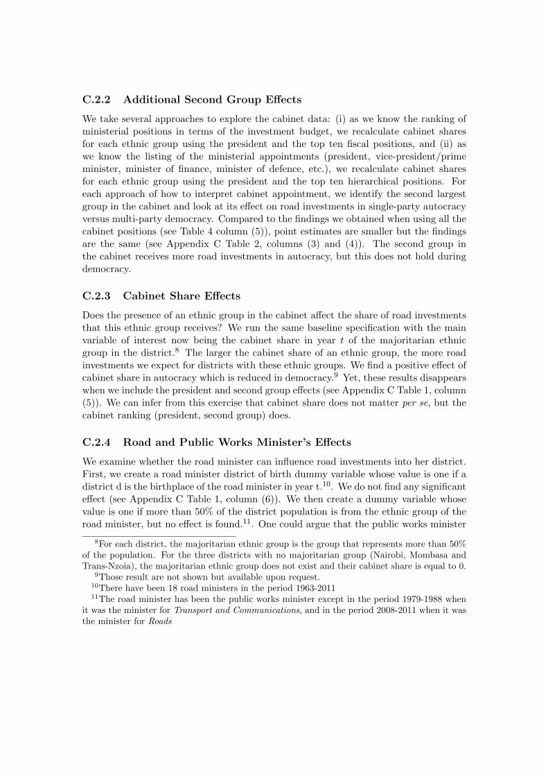
C.2.2 Additional Second Group Effects

We take several approaches to explore the cabinet data: (i) as we know the ranking ofministerial positions in terms of the investment budget, we recalculate cabinet sharesfor each ethnic group using the president and the top ten fiscal positions, and (ii) aswe know the listing of the ministerial appointments (president, vice-president/primeminister, minister of finance, minister of defence, etc.), we recalculate cabinet sharesfor each ethnic group using the president and the top ten hierarchical positions. Foreach approach of how to interpret cabinet appointment, we identify the second largestgroup in the cabinet and look at its effect on road investments in single-party autocracyversus multi-party democracy. Compared to the findings we obtained when using all thecabinet positions (see Table 4 column (5)), point estimates are smaller but the findingsare the same (see Appendix C Table 2, columns (3) and (4)). The second group inthe cabinet receives more road investments in autocracy, but this does not hold duringdemocracy.

C.2.3 Cabinet Share Effects

Does the presence of an ethnic group in the cabinet affect the share of road investmentsthat this ethnic group receives? We run the same baseline specification with the mainvariable of interest now being the cabinet share in year t of the majoritarian ethnicgroup in the district.8 The larger the cabinet share of an ethnic group, the more roadinvestments we expect for districts with these ethnic groups. We find a positive effect ofcabinet share in autocracy which is reduced in democracy.9 Yet, these results disappearswhen we include the president and second group effects (see Appendix C Table 1, column(5)). We can infer from this exercise that cabinet share does not matter per se, but thecabinet ranking (president, second group) does.

C.2.4 Road and Public Works Minister’s Effects

We examine whether the road minister can influence road investments into her district.First, we create a road minister district of birth dummy variable whose value is one if adistrict d is the birthplace of the road minister in year t.10. We do not find any significanteffect (see Appendix C Table 1, column (6)). We then create a dummy variable whosevalue is one if more than 50% of the district population is from the ethnic group of theroad minister, but no effect is found.11. One could argue that the public works minister

8For each district, the majoritarian ethnic group is the group that represents more than 50%of the population. For the three districts with no majoritarian group (Nairobi, Mombasa andTrans-Nzoia), the majoritarian ethnic group does not exist and their cabinet share is equal to 0.

9Those result are not shown but available upon request.10There have been 18 road ministers in the period 1963-201111The road minister has been the public works minister except in the period 1979-1988 when

it was the minister for Transport and Communications, and in the period 2008-2011 when it wasthe minister for Roads

has the real power when it comes to road building. There have been 21 public workministers in 1963-2011. Likewise, we create a district dummy whose value is one if it isthe district of birth of the public works minister and a district dummy whose value is oneif more than 50% of the district population matches the ethnic group of this minister.We do not find any effect.

C.3 Additional Results using Cabinet Data

We study how democracy affects the distribution of cabinet positions between the pres-idential group, the second group and other groups. The hypothesis we test is whetherthe president favors her ethnic group in terms of allocating cabinet positions. We runpanel data regressions for ethnic group e and years t of the following form:

Cpope,t = γg + αt + βPresgroupe,t + δ[Presgroupe,t ×Multipartyt] + ue,t (1)

where Cpope,t is our index of cabinet favoritism which we define as the ratio betweenthe share of cabinet positions allocated to ethnic group e in year t and the populationshare of that ethnic group in 1962. Presgroupe,t is a dummy variable whose value is oneif the ethnic group e matches with the president’s ethnic group in year t. Multipartytis a dummy variable whose value is one if the year t is a year with multi-party. Thus,β captures the effect of being a presidential ethnic group on cabinet positions in single-party autocracy, while β + δ captures this effect in multi-party democracy. γg and αt

are ethnic group and year fixed effects. Lastly, ug,t are individual disturbances clusteredat the ethnic group level.12

As explained in section C.2.2, we also have data on the ranking of cabinet positionsin terms of investment budget and official listing. We alternatively use cabinet sharedata considering the president and the top ten fiscal positions, and the president andthe top ten hierarchical positions. Results reported in Appendix C Table 3 all includean ethnic group time trend. In single-party autocracy, the presidential group gets 1.64times more cabinet positions than its population share (column (1)). Given an averagepopulation share of 15.1, this means the presidential group obtains on average 24.8%of cabinet positions. This effect increases if we consider the top hierarchical and fiscalpositions, which is logical if the president gives the best positions to her own ethnic group.For instance, the presidential group obtains 2.28 times more top fiscal positions than itspopulation share (column (2)). Surprisingly, democracy does not modify this distributionas the interaction of the presidential and multi-party dummies is zero and insignificant.We further investigate whether the second cabinet group obtains more positions (or less)in multi-party democracy. We use all positions to define the second group. By definition,the second cabinet group has more positions than the third cabinet group, the fourthcabinet group, etc. Interestingly, the interaction of the second cabinet group and multi-party dummy is insignificant. Thus, we cannot reject the hypothesis that democracy

12Regressions are run on 13 ethnic groups (12 African ethnic groups and non-Africans) overthe period 1963-2011 which results in 13 cabinet years and hence 169 observations.

cancels the effect for the second cabinet group. The previous analysis indicates thatthe cabinet structure is not significantly modified between autocracy and democracy.Distributive politics in autocracy does not come from more political representation forpowerful groups but from less checks and balances against their power. This is consistentwith not finding any independent effect of the cabinet share once we control for beingthe group of the president and the second group (see section C.2.3).

References

Bester, A., T. Conley, and C. Hansen (2011): “Inference with Dependent

Data Using Cluster Covariance Estimators,” Journal of Econometrics, Forth-

coming.

Conley, T. G. (1999): “GMM estimation with cross sectional dependence,”

Journal of Econometrics, 92(1), 1–45.

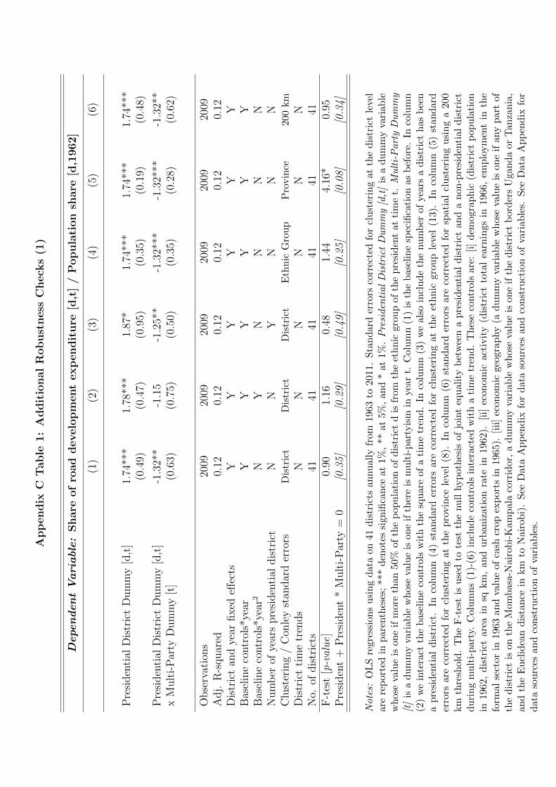
App

endix

CT

able

1:

Addit

ional

Robust

ness

Check

s(1

)

DependentVariable:

Share

of

road

develo

pm

ent

exp

endit

ure

[d,t

]/

Pop

ula

tion

share

[d,1

962]

(1)

(2)

(3)

(4)

(5)

(6)

Pre

siden

tial

Dis

tric

tD

um

my

[d,t

]1.

74**

*1.

78**

*1.

87*

1.74

***

1.74

***

1.74

***

(0.4

9)(0

.47)

(0.9

5)(0

.35)

(0.1

9)(0

.48)

Pre

siden

tial

Dis

tric

tD

um

my

[d,t

]-1

.32*

*-1

.15

-1.2

5**

-1.3

2***

-1.3

2***

-1.3

2**

xM

ult

i-P

arty

Dum

my

[t]

(0.6

3)(0

.75)

(0.5

0)(0

.35)

(0.2

8)(0

.62)

Obse

rvat

ions

2009

2009

2009

2009

2009

2009

Adj.

R-s

quar

ed0.

120.

120.

120.

120.

120.

12D

istr

ict

and

year

fixed

effec

tsY

YY

YY

YB

asel

ine

contr

ols*

year

YY

YY

YY

Bas

elin

eco

ntr

ols*

year

2N

YN

NN

NN

um

ber

ofye

ars

pre

siden

tial

dis

tric

tN

NY

NN

NC

lust

erin

g/

Con

ley

stan

dar

der

rors

Dis

tric

tD

istr

ict

Dis

tric

tE

thnic

Gro

up

Pro

vin

ce200

km

Dis

tric

tti

me

tren

ds

NN

NN

NN

No.

ofdis

tric

ts41

4141

4141

41F

-tes

t[p-value]

0.90

1.16

0.48

1.44

4.16

*0.

95P

resi

den

t+

Pre

siden

t*

Mult

i-P

arty

=0

[0.35]

[0.29]

[0.49]

[0.25]

[0.08]

[0.34]

Notes:

OL

Sre

gre

ssio

ns

usi

ng

dat

aon

41d

istr

icts

an

nu

ally

from

1963

to20

11.

Sta

nd

ard

erro

rsco

rrec

ted

for

clu

ster

ing

atth

ed

istr

ict

leve

lare

rep

ort

edin

pare

nth

eses

;***

den

ote

ssi

gn

ifica

nce

at1%

,**

at5%

,an

d*

at1%

.Presiden

tialDistrictDummy[d,t]

isa

du

mm

yva

riab

lew

hos

eva

lue

ison

eif

more

than

50%

of

the

pop

ula

tion

ofd

istr

ict

dis

from

the

eth

nic

grou

pof

the

pre

sid

ent

atti

me

t.Multi-PartyDummy

[t]

isa

du

mm

yva

riab

lew

hose

valu

eis

one

ifth

ere

ism

ult

i-p

arty

ism

inyea

rt.

Col

um

n(1

)is

the

bas

elin

esp

ecifi

cati

on

asb

efore

.In

colu

mn

(2)

we

inte

ract

the

base

lin

eco

ntr

ols

wit

hth

esq

uare

ofa

tim

etr

end

.In

colu

mn

(3)

we

also

incl

ud

eth

enu

mb

erof

yea

rsa

dis

tric

th

as

bee

na

pre

siden

tial

dis

tric

t.In

colu

mn

(4)

stan

dar

der

rors

are

corr

ecte

dfo

rcl

ust

erin

gat

the

eth

nic

gro

up

leve

l(1

3).

Inco

lum

n(5

)st

an

dard

erro

rsar

eco

rrec

ted

for

clu

ster

ing

at

the

pro

vin

cele

vel

(8).

Inco

lum

n(6

)st

and

ard

erro

rsare

corr

ecte

dfo

rsp

ati

alcl

ust

erin

gu

sin

ga

200

km

thre

shold

.T

he

F-t

est

isu

sed

tote

stth

enu

llhyp

oth

esis

ofjo

int

equ

alit

yb

etw

een

ap

resi

den

tial

dis

tric

tan

da

non

-pre

sid

enti

al

dis

tric

td

uri

ng

mu

lti-

par

ty.

Colu

mn

s(1

)-(6

)in

clu

de

contr

ols

inte

ract

edw

ith

ati

me

tren

d.

Th

ese

contr

ols

are

:[i

]d

emogr

ap

hic

(dis

tric

tp

op

ula

tion

in1962

,d

istr

ict

area

insq

km

,an

du

rban

izati

onra

tein

1962

).[i

i]ec

onom

icac

tivit

y(d

istr

ict

tota

lea

rnin

gs

in19

66,

emp

loym

ent

inth

efo

rmal

sect

orin

1963

an

dva

lue

ofca

shcr

op

exp

orts

in19

65).

[iii

]ec

onom

icge

ogra

phy

(ad

um

my

vari

ab

lew

hose

valu

eis

on

eif

any

part

of

the

dis

tric

tis

onth

eM

omb

asa

-Nair

obi-

Kam

pal

aco

rrid

or,

ad

um

my

vari

able

wh

ose

valu

eis

on

eif

the

dis

tric

tb

ord

ers

Ugan

da

or

Tan

zan

ia,

an

dth

eE

ucl

idea

nd

ista

nce

inkm

toN

airo

bi)

.S

eeD

ata

Ap

pen

dix

for

dat

aso

urc

esan

dco

nst

ruct

ion

ofva

riab

les.

See

Data

Ap

pen

dix

for

dat

aso

urc

esan

dco

nst

ruct

ion

ofva

riab

les.

Appendix C Table 2: Additional Robustness Checks (2)

Dependent Variable: Share of road dvt expenditure [d,t] / Population share [d,1962]

(1) (2) (3) (4) (5) (6)

Presidential District Dummy [d,t] 1.74*** 2.62*** 1.89*** 2.13*** 2.30** 1.73***(0.49) (0.71) (0.50) (0.56) (0.85) (0.49)

Presidential District Dummy [d,t] -1.32** -1.63** -1.43** -1.43** -2.27* -1.33**x Multi-Party Dummy [t] (0.63) (0.69) (0.64) (0.64) (1.17) (0.62)

Vice-Presidential District Dummy [d,t] 1.46**(0.56)

Vice-Presidential District Dummy [d,t] -1.42**x Multi-Party Dummy [t] (0.61)

Second Cabinet Group [d,t], Fiscal 1.01*(0.52)

Second Cabinet Group [d,t], Fiscal -1.20**x Multi-Party Dummy [t] (0.59)

Second Cabinet Group [d,t], Hierarchy 1.09**(0.42)

Second Cabinet Group [d,t], Hierarchy -0.98*x Multi-Party Dummy [t] (0.55)

Second Cabinet Group [d,t], All Positions 1.66**(0.73)

Second Cabinet Group [d,t], All Positions -2.50**x Multi-Party Dummy [t] (1.19)

Cabinet Share of Maj. Ethnic Group [d,t] 0.02(0.04)

Cabinet Share of Maj. Ethnic Group [d,t] 0.04x Multi-Party Dummy [t] (0.05)

Road Minister District of Birth [d,t] 0.62(0.47)

Road Minister District of Birth [d,t] -0.32x Multi-Party Dummy [t] (0.82)

Observations 2009 2009 2009 2009 2009 2009Adj. R-squared 0.12 0.12 0.13 0.12 0.12 0.13District and year fixed effects Y Y Y Y Y YBaseline controls*year Y Y Y Y Y YDistrict time trends N N N N N NNo. of districts 41 41 41 41 41 41

F-test [p-value] 0.90 2.64 1.12 2.50 0.00 0.81President + President * Multi-Party = 0 [0.35] [0.11] [0.30] [0.12] [0.97] [0.37]

Notes: OLS regressions using data on 41 districts annually from 1963 to 2011. Standard errors corrected forclustering at the district level are reported in parentheses; *** denotes significance at 1%, ** at 5%, and * at1%. Presidential District Dummy [d,t] is a dummy equal to one if more than 50% of the population of districtd is from the ethnic group of the president at time t. Multi-Party Dummy [t] is a dummy equal to one if thereis multi-partyism in year t. Vice-Presidential District Dummy [d,t] is a dummy variable whose value is one ifmore than 50% of the population of district d is from the ethnic group of the vice-president at time t. SecondCabinet Group [d,t] is a dummy variable whose value is one if more than 50% of the population of district d isfrom the second largest group in the cabinet at time t. Fiscal, Hierarchy and All Positions denote that we usethe president and the top ten fiscal positions, top ten hierarchical positions, or all the positions. Cabinet Shareof Maj. Ethnic Group [d,t] is the cabinet share at time t of the majoritatian group in district d. Road MinisterDistrict of Birth [d,t] is a dummy variable whose value is one if district d is the district of birth of the roadminister at time t. The F-test is used to test the null hypothesis of joint equality between a presidential districtand a non-presidential district during multi-party. Control variables are defined as before. See Data Appendixfor data sources and construction of variables.

App

endix

CT

able

3:

Expla

inin

gC

abin

et

Eth

nic

Share

DependentVariable:

Cabin

et

eth

nic

share

[e,t

]/

Popula

tion

share

[e,1

962]

Cab

inet

sam

ple

:A

llF

isca

lH

iera

rchy

All

Fis

cal

Hie

rarc

hy

(1)

(2)

(3)

(4)

(5)

(6)

Pre

siden

tial

Gro

up

Dum

my

[e,t

]0.

64**

*1.

18**

0.82

**0.

90**

*1.

36**

1.05

*[0

.13]

[0.5

4][0

.27]

[0.2

6][0

.51]

[0.5

2]

Pre

siden

tial

Gro

up

Dum

my

[e,t

]0.

02-0

.10

-0.2

40.

11-0

.03

-0.2

2x

Mult

i-P

arty

Dum

my

[t]

[0.2

8][0

.51]

[0.4

7][0

.33]

[0.5

4][0

.51]

Sec

ond

Cab

inet

Gro

up

[e,t

]1.

00**

*0.

710.

75[0

.17]

[0.4

7][0

.86]

Sec

ond

Cab

inet

Gro

up

[e,t

]-0

.59

-0.3

5-0

.96

xM

ult

i-P

arty

Dum

my

[t]

[0.4

4][1

.07]

[1.3

8]

Obse

rvat

ions

169

169

169

169

169

169

Adj.

R-s

quar

ed0.

560.

200.

230.

580.

190.

22E

thnic

grou

pan

dye

arfixed

effec

tsY

YY

YY

YG

roup

tim

etr

ends

YY

YY

YY

No.

ofet

hnic

grou

ps

1313

1313

1313

F-t

est

[p-value]

5.9*

*11

.6**

*9.

1**

204.

6***

84.0

***

4.0*

Pre

siden

t+

Pre

siden

t*

Mult

i-P

arty

=0

[0.03]

[0.00]

[0.01]

[0.00]

[0.00]

[0.07]

Notes:

OL

Sre

gres

sion

su

sin

gdat

aon

all

elec

tion

sfr

om19

63to

2011

,fo

r13

grou

ps

(tw

elve

Afr

ican

eth

nic

grou

ps

and

an

oth

erca

tegory

[Asi

an

s,A

rab

s,N

on-K

enya

ns]

).S

tan

dar

der

rors

corr

ecte

dfo

rcl

ust

erin

gat

the

eth

nic

grou

ple

vel

are

rep

orte

din

par

enth

eses

;***

den

ote

ssi

gnifi

can

ceat

1%,

**at

5%,

and

*at

10%

.T

he

dep

end

ent

vari

able

Cabinet

Ethnic

Share

[e,t]/PopulationShare

[e,1962]

isd

efin

edas

the

rati

ob

etw

een

the

cab

inet

shar

eof

eth

nic

grou

pe

atti

me

tto

the

nat

ion

alp

opu

lati

onsh

are

ofet

hn

icgr

oup

ein

1962.Presiden

tial

GroupDummy[e,t]

isa

du

mm

yva

riab

lew

hos

eva

lue

ison

eif

eth

nic

grou

pe

isth

egr

oup

ofth

ep

resi

den

t.Multi-partyDummy[t]

isa

du

mm

yva

riab

lew

hos

eva

lue

ison

eif

ther

eis

mu

lti-

par

tyis

min

year

t.SecondCabinet

Group[e,t]

isd

um

my

vari

able

wh

ose

valu

eis

on

eif

eth

nic

gro

up

eis

the

seco

nd

larg

est

grou

pin

the

cab

inet

.In

colu

mn

s(1

)an

d(4

),th

ed

epen

den

tva

riab

leco

nsi

der

sal

lca

bin

etp

osi

tion

s.In

colu

mn

s(2

)an

d(5

),th

ed

epen

den

tva

riab

leco

nsi

der

sth

eca

bin

etsh

are

usi

ng

the

pre

sid

ent

and

the

top

ten

fisc

alp

osit

ion

s.In

colu

mn

s(3

)an

d(6

),th

ed

epen

den

tva

riab

leco

nsi

der

sth

eca

bin

etsh

are

usi

ng

the

pre

sid

ent

and

the

top

ten

hie

rarc

hic

alp

osit

ion

s(a

ccord

ing

toth

eli

stp

rovid

edby

the

Offi

ceof

the

Pre

sid

ent)

.T

he

F-t

est

isu

sed

tote

stth

enu

llhyp

oth

esis

ofjo

int

equ

alit

yb

etw

een

ap

resi

den

tial

dis

tric

tan

da

non

-pre

siden

tial

dis

tric

td

uri

ng

mu

lti-

par

ty.

See

Dat

aA

pp

end

ixfo

rd

ata

sou

rces

and

con

stru

ctio

nof

vari

able

s.