Ethnic Inequality∗

Alberto Alesina

Harvard University, IGIER, CEPR, and NBER

Stelios Michalopoulos

Brown University, and NBER

Elias Papaioannou

London Business School, CEPR, and NBER

First Draft: October 2012

Revised April and then October 2014

Abstract

This study explores the consequences and origins of between-ethnicity economic inequality

across countries. First, combining satellite images of nighttime luminosity with the historical

homelands of ethnolinguistic groups we construct measures of ethnic inequality for a large sam-

ple of countries. We also compile proxies of overall spatial inequality and regional inequality

across administrative units. Second, we uncover a strong negative association between ethnic

inequality and contemporary comparative development; the correlation is also present when

we condition on regional inequality, which is itself related to under-development. Third, we

investigate the roots of ethnic inequality and establish that differences in geographic endow-

ments across ethnic homelands explain a sizable fraction of the observed variation in economic

disparities across groups. Fourth, we show that ethnic-specific inequality in geographic en-

dowments is also linked to under-development.

Keywords: Ethnicity, Diversity, Inequality, Development, Geography

JEL classification Numbers: O10, O40, O43.

∗We thank Harald Uhlig (the Editor) and two anonymous referees for excellent comments. We would like

to thank Nathan Fleming and Sebastian Hohmann for superlative research assistance. For valuable suggestions

we also thank Christian Dippel, Oeindrila Dube, Sebastian Hohmann, Michele Lenza, Nathan Nunn, Debraj Ray,

Andrei Shleifer, Enrico Spolaore, Pierre Yared, Romain Wacziarg, David Weil, Ivo Welch, and seminar participants

at Dartmouth, the Athens University of Economics and Business, UBC, Brown, CREi, Oxford, Bocconi, NYU,

Michigan, Paris School of Economics, IIES, Columbia, KEPE, Warwick, LSE, Nottingham, the NBER Summer

Institute Meetings in Political Economy, the CEPR Development Economics Workshop, the conference "How

Long is the Shadow of History? The Long-Term Persistence of Economic Outcomes" at UCLA, and the Nemmers

Conference in the Political Economy of Growth and Development at Northwestern University. Papaioannou greatly

acknowledges financial support from the LBS RAMD fund. All errors are our own responsibility.

0

1 Introduction

Ethnic diversity has costs and benefits. On the one hand, diversity in skills, education, and

endowments can enhance productivity by promoting innovation. On the other hand, diversity is

often associated with poor and ethnically targeted policies, inefficient provision of public goods,

and ethnic-based hatred and conflict. In fact, a large literature finds a negative impact of ethno-

linguistic fragmentation on various aspects of economic performance, with the possible exception

of wealthy economies (see Alesina and Ferrara (2005) for a review). Income inequality may also

have both positive and negative effects on development. On the negative side, a higher degree

of income inequality may lead to conflict and crime, prevent the poor from acquiring educa-

tion, and/or lead to expropriation and lofty taxation discouraging investment. On the positive

side, income inequality may spur innovation and entrepreneurship by motivating individuals and

by providing the necessary pools of capital for capital-intensive modes of production. Further

complicating the relationship between the two, a positive correlation between inequality and de-

velopment may reflect Simon Kuznetz’s conjecture that industrialization translates into higher

levels of inequality at the early stages of development; while at later stages, the association be-

comes negative. Given the theoretical ambiguities (and data issues), perhaps it comes at no

surprise that it has been very hard to detect empirically a robust association between inequality

and development (see Benabou (2005) and Galor (2011) for surveys).

This paper puts forward and tests an alternative conjecture that focuses on the intersection

of ethnic diversity and inequality. Our thesis is that what matters most for comparative devel-

opment are economic differences between ethnic groups coexisting in the same country, rather

than the degree of fractionalization per se or income inequality conventionally measured (i.e.,

independent of ethnicity).1

The first contribution of this study is to provide measures of within-country differences in

well-being across ethnic groups, defined as "ethnic inequality." To overcome the sparsity of income

data along ethnic lines and in order to construct country-level indicators of ethnic inequality for

the largest possible set of states, we combine ethnographic and linguistic maps on the location

of groups with satellite images of light density at night which are available at a fine grid. Recent

studies have shown that luminosity is a strong proxy of development (e.g., Henderson, Storeygard,

and Weil (2012)). The cross-ethnic group inequality index is weakly correlated with the commonly

employed —and notoriously poorly measured— income inequality measures at the country level and

is modestly correlated with ethnic fractionalization. To isolate the cross-ethnic component of

1Stewart (2002) and Chua (2003) are early precedents. Providing case-study evidence, they argue that horizon-

tal inequalities across ethnic/religious/racial groups are important features of underdeveloped and conflict-prone

societies. Yet to the best of our knowledge, there have been very few systematic empirical works —if any— that

directly examine this conjecture. We discuss parallel studies that touch upon this issue below.

1

inequality from the overall regional inequality, we also construct proxies of spatial inequality and

measures capturing regional differences in well-being across first and second-level administrative

units.

Second, we document a strong negative association between ethnic inequality and real GDP

per capita across countries. This correlation holds even when we control for the overall degree of

spatial inequality and inequality across administrative regions. The latter is also inversely related

to a country’s economic performance, a novel finding in itself. We also uncover that the negative

correlation between ethnolinguistic fragmentation and development weakens considerably (and

becomes statistically indistinguishable from zero) when we account for ethnic inequality; this

suggests that it is the unequal concentration of wealth across ethnic lines that correlates with

development rather than diversity per se.

Third, in an effort to shed light on the roots of ethnic inequality, we explore its geographic

underpinnings. In particular, motivated by recent work showing that linguistic groups tend to

reside in distinct land endowments, see Michalopoulos (2012), we construct Gini coefficients re-

flecting differences in various geographic attributes across ethnic homelands and show that the

latter is a strong predictor of ethnic inequality. On the contrary, there is no link between con-

temporary ethnic inequality and often-used historical variables capturing the type of colonization

and legal origin among others.

Fourth, we show that contemporary development at the country level is also inversely re-

lated to inequality in geographic endowments across ethnic homelands. Yet, once we condition

on between-group income inequality, differences in geographic endowments are no longer a sig-

nificant correlate of underdevelopment. These results suggest that geographic differences across

ethnic homelands influence comparative development mostly via shaping economic inequality

across groups.

Mechanisms and Related Works Income disparities along ethnic lines are likely to

lead to political inequality based on ethnic affiliation, increase between-group animosity, and lead

to discriminatory policies of one (or more) groups against the others. In line with this idea, in

recent work Huber and Suryanarayan (2013) document that party ethnification in India is more

pronounced in states with a high degree of inequality across sub-castes.2 Furthermore, differences

2Ethnic inequality may impede development by spurring civil conflict (Horowitz (1985)). However, Esteban and

Ray (2011) show that the effect of ethnic inequality on conflict is ambiguous, as it also depends on within-group

inequality. Recent works in political science provide opposing results. Cederman, Weidman, and Gleditch (2011)

combine proxies of local economic activity from the G-Econ database with ethnolinguistic maps to construct an

index of ethnic inequality for a sub-set of "politically relevant ethnic groups" (as defined by the Ethnic Power

Relations Dataset) and then show that in highly unequal countries, both rich and poor groups fight more often

than those groups whose wealth is closer to the country average. However, in parallel work Huber and Mayoral

(2013) find no link between inequality across ethnic lines and conflict.

2

in preferences along both ethnic and income lines may lead to inadequate public goods provision,

as groups’ ideal allocations of resources will be quite distant. Baldwin and Huber (2010) provide

empirical evidence linking between-group inequality to the under-provision of public goods for 46

democracies. In Alesina, Michalopoulos, and Papaioannou (2014), we show that there is a strong

inverse link between ethnic inequality and public goods within 18 Sub-Saharan African countries

(and that this effect partly stems from political inequality and ethnic-based discrimination).3

Ethnic inequality may also impede institutional development and the consolidation of democracy

(Robinson (2001)). In line with this conjecture, Kyriacou (2013) exploits survey data from 29

developing countries and shows that socioeconomic ethnic-group inequalities reduce government

quality.

Chua (2003) presents case-study evidence arguing that the presence of an economically

dominant ethnic minority may lower support for democracy and free-market institutions, as the

majority of the population usually feels that the benefits of capitalism go to just a handful of

ethnic groups. She discusses, among others, the influence of Chinese minorities in the Philippines,

Indonesia, Malaysia, and other Eastern Asian countries; the dominant role of (small) Lebanese

communities in Western Africa; and the similarly strong influence of Indian societies in Eastern

Africa. Other examples, include the I(g)bo in Nigeria and the Kikuyu in Kenya. Finally, to the

extent that ethnic inequality implies that well-being depends on one’s ethnic identity, then it is

more likely to generate envy and perceptions that the system is "unfair," and reduce interpersonal

trust, more so than the conventionally measured economic inequality, since the latter can be more

easily thought of as the result of ability or effort. Consistent with the view that ethnic inequality

is detrimental to the formation of social ties across groups, Tesei (2014) finds that greater racial

inequality across US metropolitan areas is associated with low levels of social capital.

Organization The paper is organized as follows. In section 2 we describe the construc-

tion of the ethnic (and regional) inequality measures and present summary statistics and the

basic correlations. In section 3 we report the results of our analysis associating income per

capita with ethnic inequality across 173 countries. Besides reporting various sensitivity checks,

we also examine the link between development and inequality across administrative regions. In

section 4 we explore the geographic origins of contemporary differences in economic performance

across groups. In section 5 we report estimates associating contemporary development with in-

equality in geographic endowments across ethnic homelands. In the last section, we summarize

our findings and discuss avenues for future research.

3Similarly, Deshpande (2000) and Anderson (2011) focus on income inequality across castes in India and asso-

ciate between-caste inequality to public goods provision. See also Loury (2002) for an overview of works studying

the evolution of racial inequality in the US and its implications.

3

2 Data

To construct proxies of ethnic inequality for the largest set of countries, we combine information

from ethnographic/linguistic maps on the location of groups with satellite images of light density

at night that are available at a fine grid. In this section, we discuss the construction of the cross-

country measures reflecting inequality in development (as captured by luminosity per capita)

across ethnic homelands within 173 countries. We also describe in detail the construction of the

other measures of spatial inequality and discuss the main patterns.

2.1 Ethnic Inequality Measures

2.1.1 Location of Ethnic Groups

We identify the location of ethnic groups employing two data sets/maps.4 First, we use the Geo-

referencing of Ethnic Groups (GREG), which is the digitized version of the Soviet Atlas Narodov

Mira (Weidmann, Rod, and Cederman (2010)). GREG portrays the homelands of 928 ethnic

groups around the world. The information pertains to the early 1960s, so for many countries,

in Africa in particular and to a lesser extent in South-East Asia, it corresponds to the time of

independence.5 The data set uses the political boundaries of 1964 to allocate groups to different

countries. We thus project the ethnic homelands to the political boundaries of the 2000 Digital

Chart of the World; this results in 2 129 ethnic homelands within contemporary countries. Most

areas (1 637) are coded as pertaining to a single group, whereas in the remaining 492 homelands,

there can be up to three overlapping groups. For example, in Northeast India over an area of

4 380 2, the Assamese, the Oriyas and the Santals overlap. The luminosity of a region where

multiple groups reside contributes to the average luminosity of each group. The size of ethnic

homelands varies considerably. The smallest polygon occupies an area of 109 km2 (French in

Monaco), and the largest extends over 7 335 476 km2 (American English in the US). The median

(mean) group size is 4 183 (61 213) km2. The median (mean) country in our sample has 8 (115)

ethnicities with the most diverse being Indonesia with 95 groups.

Our second source is the 15th edition of the Ethnologue (Gordon (2005)) that maps 7 581

language-country groups worldwide in the mid/late 1990s, using the political boundaries of 2000.

In spite of the comprehensive linguistic mapping, Ethnologue’s coverage of the Americas and

Australia is rather limited while for others (i.e., Africa and Asia), it is very detailed. Each

polygon delineates a traditional linguistic region; populations away from their homelands (in

4Note that across all units of analysis in the construction of the respective indexes we exclude polygons of less

than 1 square kilometer to minimize measurement error in the drawing of the underlying maps.5The original Atlas Narodov Mira consists of 57maps. The original sources are: (1) ethnographic and geographic

maps assembled by the Institute of Ethnography at the USSR Academy of Sciences, (2) population census data,

and (3) ethnographic publications of government agencies at the time.

4

cities, refugee camps) are not mapped. Groups of unknown location, as well as widespread and

extinct languages are not mapped either, the only exception is the English in the United States.

Ethnologue also records areas where languages overlap. Ethnologue provides a more refined

linguistic aggregation compared to the GREG. As a result the median (mean) homeland extends

to 726 (12 676) km2. The smallest language is the Domari in Israel which covers 118 km2 and

the largest group is the English in the US covering 7 330 520 km2. The median (mean) country

has 9 (423) groups with Papua New Guinea being the most diverse with 809 linguistic groups.

GREG attempts to map major immigrant groups whereas Ethnologue generally does not.

This is important for countries in the New World. For example, in Argentina GREG reports

16 groups, among them Germans, Italians, and Chileans, whereas Ethnologue reports 20 purely

indigenous groups (e.g., the Toba and the Quechua). For Canada, Ethnologue lists 77 mostly

indigenous groups, like the Blackfoot and the Chipewyan with only English and French being

non-indigenous; in contrast, GREG lists 23 groups featuring many non-indigenous ones, such as

Swedes, Russians, Norwegians, and Germans. Hence, the two ethnolinguistic mappings capture

different cleavages, at least in some continents. Though we have performed various sensitivity

checks, for our benchmark results we are including all groups without attempting to make a

distinction as to which cleavage is more salient.6

It is important to note that the underlying maps do include regions where groups overlap

and we take that into account in our measure, as we show below. However, both maps do not

capture relatively recent within-country migrations towards the urban centers, for example. The

reason is that the original sources attempt to trace the historical homeland of each group. Hence,

actual ethnic mixing is likely higher than what the ethnographic maps reflect. This will induce

measurement error to our proxies of ethnic inequality. Nevertheless, under the assumption that

in a given urban center the respective indigenous group is relatively more populous than recent

migrant ones, then assigning the observed luminosity per capita to this group is not entirely ad

hoc. Moreover, there is a large literature documenting that migrant workers channel systemat-

ically a fraction of their earnings back to their homelands. This would imply that although we

do not observe migrant workers in our dataset to the extent that they send remittances to their

families and influence their livelihoods, this will be reflected in the luminosity per capita of the

ancestral homelands which we directly measure. Moreover, to at least partially account for this

issue, we have constructed all inequality measures also excluding the regions where capitals fall.

6A thorough exploration of ethnic inequality across different linguistic cleavages is relegated to the Online

Supplementary Appendix.

5

2.1.2 Data on Luminosity and Population

Comparable data on income per capita at the ethnicity level are scarce. Hence, following Hen-

derson, Storeygard, and Weil (2012) and subsequent studies (e.g., Chen and Nordhaus (2011),

Pinkovskiy (2013), Pinkovskiy and Sala-i-Martin (2014), Hodler and Raschky (2014), Michalopou-

los and Papaioannou (2013, 2014)), we use satellite image data on light density at night as a proxy.

These —and other works— show that luminosity is a strong correlate of development at various

levels of aggregation (countries, regions, ethnic homelands). The luminosity data come from the

Defense Meteorological Satellite Program’s Operational Linescan System that reports images of

the earth at night (from 20:30 till 22:00). The six-bit number that ranges from 0 to 63 is available

approximately at every square kilometer since 1992.

To construct luminosity at the desired level of aggregation, we average all observations

falling within the boundaries of an ethnic group and then divide by the population of each

area using data from the Gridded Population of the World that reports georeferenced pixel-level

population estimates for 1990 and 2000.7

2.1.3 New Ethnic Inequality Measures

We proxy the level of economic development in ethnic homeland with mean luminosity per

capita, ; and we then construct an ethnic Gini coefficient for each country that reflects inequal-

ity across ethnolinguistic regions. Specifically, the Gini coefficient for a country’s population

consisting of groups with values of luminosity per capita for the historical homeland of group

, , where = 1 to are indexed in non-decreasing order ( ≤ +1), is calculated as follows:

=1

µ+ 1− 2

P=1(+ 1− )P

=1

¶The ethnic Gini index captures differences in mean income —as captured by luminosity per

capita at the ethnic homeland— across groups. For each of the two different ethnic-linguistic maps

(Atlas Narodov Mira and Ethnologue) we construct Gini coefficients for the maximum sample

of countries using cross-ethnic-homeland data in 1992, 2000, and 2012. For each mapping we

construct three ethnic Ginis. First, for our baseline estimates we use information from all groups.

Second, we construct the Gini coefficient dropping the capital cities. This allows us to account

both for extreme values in luminosity and also for population mixing which is naturally higher in

capitals. Third, we compile measures excluding small ethnicities, defined as those representing

less than 1% of the 2000 population in a country.8

7The data is constructed using subnational censuses and other population surveys at various levels (city, neigh-

borhood, region). See for details: http://sedac.ciesin.columbia.edu/data/collection/gpw-v

In the online Supplementary Appendix, we present various sensitivity checks that examine the role of measure-

ment error both in the population estimates and the luminosity data.8For example, in Kenya the Atlas Narodov Mira (the Ethnologue) maps 19 (53) ethnic (linguistic) groups. Yet

6

2.2 Measures of Spatial Inequality

Since we use ethnic homelands (rather than individual-level) data to measure between-group

inequality, the ethnic inequality measures also reflect regional disparities in income and/or public

goods provision that may not be related to ethnicity per se. To isolate the between-ethnicity

component of inequality from the regional one, we also construct Gini coefficients reflecting (i) the

overall degree of spatial inequality and (ii) inequality across (first and second level) administrative

units for each country. Moreover, in an attempt to assess the accuracy of the underlying groups’

mappings, we perturbed the original homelands and compiled Gini coefficients based on these

altered ethnic homelands.

2.2.1 Overall Spatial Inequality Index

Our baseline index reflecting the overall degree of spatial inequality is based on aggregating (via

the Gini coefficient formula) luminosity per capita across roughly equally-sized pixels in each

country. We first generate a global grid of 25 x 25 decimal degrees (that extends from −180to 180 degrees longitude and from 75 degrees latitude to −65 degrees latitude). Second, weintersect the resulting grid with the 2000 Digital Chart of the World that portrays contemporary

national borders. This results in 4 865 pixels across the globe falling within country boundaries.

The median (mean) box extends to 22 438 (27 622) km2, being comparable to the size of ethnic

homelands in the GREG dataset, when we exclude small groups. Note that boxes intersected by

the coastline and national boundaries are smaller. Third, for each box we compute luminosity

per capita in 1992, 2000, and 2012. Fourth, we aggregate the data at the country level estimating

a Gini coefficient that captures the overall degree of spatial inequality. The cross-country mean

(median) number of pixels used for the estimation of the spatial Ginis is 249 (8); so these Ginis

are quite comparable to the ethnic inequality measures.

2.2.2 Inequality across Administrative Regions

We also compiled inequality measures across administrative units, using data from the GADM

Global Administrative Areas database on the boundaries of administrative regions. Following

a similar procedure to the derivation of the ethnic inequality and the overall spatial inequality

indexes, we construct measures reflecting inequality (in lights per capita) across first-level and

second-level administrative units. In our sample of 173 countries, the median (mean) number

of first-level administrative units is 13 (17). A median (mean) first-level administrative unit

8 ethnic (37 linguistic) areas host less than one percent of Kenya’s population as of 2000. So, we construct Gini

coefficients (i) using all ethnic groups (19 and 53), (ii) dropping ethnic regions where the capital (Nairobi) falls

(18 and 52), and (iii) using the 11 ethnic and 16 linguistic groups, respectively, whose populations exceed 1% of

Kenya’s population.

7

spans roughly 7 197 (44 050) square kilometers, which is somewhat larger than the median size

(4 578) for groups in the Atlas Narodov Mira. The cross-country median (mean) size of second-

level administrative units is 110 (301) 2. So, these units are much smaller than the Ethnologue

or the Atlas Narodov Mira homelands.

2.2.3 Inequality across Perturbed Ethnic Regions

We have also created ethnic Gini coefficients using perturbed ethnic regions. Using as inputs

the centroids of ethnic-linguistic homelands, we generate Thiessen polygons that have the unique

property that each polygon contains only one input point and that any location within a polygon

is closer to its associated point than to a point within any other polygon. Thiessen polygons

have the exact same centroids as the actual linguistic and ethnic homelands in the Ethnologue

and GREG databases, respectively; the key difference being that the actual homelands have

idiosyncratic shapes.9 We then construct a spatial Gini coefficient that reflects inequality in

lights per capita across these sets of Thiessen polygons. The mean size of the Thiessen polygons

based on the Ethnologue (GREG) database is 11 862 (58 784) km2, very similar to the mean size

of homelands in the Ethnologue (GREG) —12 676 (61 213) km2.

Comment All three proxies of the spatial inequality also reflect inequality across ethnic

homelands, since (i) there is clearly some degree of measurement error on the exact boundaries

of ethnic regions, (ii) population mixing is likely higher than the one we observe in the data.

Moreover, in several countries, administrative boundaries follow ethnic lines, while in the case

of large groups, the spatial Gini coefficients may also (partially) capture within-ethnic-group

inequality.10

2.3 Example

Figures 1 and 2 provide an illustration of the construction of the ethnic inequality measures for

Afghanistan. The Atlas Narodov Mira (GREG) maps 31 ethnicities (Figure 1) whereas the

Ethnologue reports 39 languages (Figure 2). According to GREG, the Afghan (Pashtuns) is the

largest group residing in the southern and central-southern regions. This group makes up 51% of

9Note that there are very few instances in which the number of Thiessen polygons is not identical to the number

of the underlying groups (for example, there is a difference of one group for 6 out of the 173 countries in the

Ethnologue). This difference is due to the fact that a handful of border/coastal groups have such a peculiar shape

that their centroid falls out of the country’s boundaries they belong to. Hence, since Thiessen polygons are based

on the centroids of the ethnic-linguistic groups that fall within the country, those groups whose centroids fall

outside are not taken into account. Note that this has virtually no effect on the results since when we focus on the

countries where the number of Thiessen polygons is identical to the number of groups the pattern is the same.10 In principle one could generate within-group inequality measures using the finer structure of the luminosity

data. However, within-group mobility and risk sharing issues make a luminosity-based, within-group inequality

index less satisfactory.

8

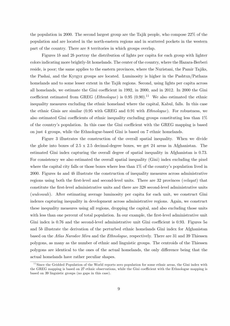
the population in 2000. The second largest group are the Tajik people, who compose 22% of the

population and are located in the north-eastern regions and in scattered pockets in the western

part of the country. There are 8 territories in which groups overlap.

Figures 1 and 2 portray the distribution of lights per capita for each group with lighter

colors indicating more brightly-lit homelands. The center of the country, where the Hazara-Berberi

reside, is poor; the same applies to the eastern provinces, where the Nuristani, the Pamir Tajiks,

the Pashai, and the Kyrgyz groups are located. Luminosity is higher in the Pashtun/Pathans

homelands and to some lesser extent in the Tajik regions. Second, using lights per capita across

all homelands, we estimate the Gini coefficient in 1992, in 2000, and in 2012. In 2000 the Gini

coefficient estimated from GREG (Ethnologue) is 095 (090).11 We also estimated the ethnic

inequality measures excluding the ethnic homeland where the capital, Kabul, falls. In this case

the ethnic Ginis are similar (095 with GREG and 091 with Ethnologue). For robustness, we

also estimated Gini coefficients of ethnic inequality excluding groups constituting less than 1%

of the country’s population. In this case the Gini coefficient with the GREG mapping is based

on just 4 groups, while the Ethnologue-based Gini is based on 7 ethnic homelands.

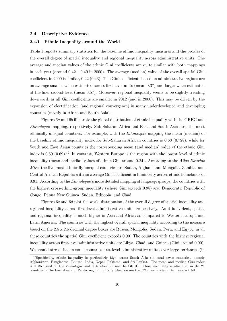
Figure 3 illustrates the construction of the overall spatial inequality. When we divide

the globe into boxes of 25 x 25 decimal-degree boxes, we get 24 areas in Afghanistan. The

estimated Gini index capturing the overall degree of spatial inequality in Afghanistan is 073.

For consistency we also estimated the overall spatial inequality (Gini) index excluding the pixel

where the capital city falls or those boxes where less than 1% of the country’s population lived in

2000. Figures 4 and 4 illustrate the construction of inequality measures across administrative

regions using both the first-level and second-level units. There are 32 provinces (velayat) that

constitute the first-level administrative units and there are 328 second-level administrative units

(wuleswali). After estimating average luminosity per capita for each unit, we construct Gini

indexes capturing inequality in development across administrative regions. Again, we construct

these inequality measures using all regions, dropping the capital, and also excluding those units

with less than one percent of total population. In our example, the first-level administrative unit

Gini index is 076 and the second-level administrative unit Gini coefficient is 093. Figures 5

and 5 illustrate the derivation of the perturbed ethnic homelands Gini index for Afghanistan

based on the Atlas Narodov Mira and the Ethnologue, respectively. There are 31 and 39 Thiessen

polygons, as many as the number of ethnic and linguistic groups. The centroids of the Thiessen

polygons are identical to the ones of the actual homelands, the only difference being that the

actual homelands have rather peculiar shapes.

11Since the Gridded Population of the World reports zero population for some ethnic areas, the Gini index with

the GREG mapping is based on 27 ethnic observations, while the Gini coefficient with the Ethnologue mapping is

based on 39 linguistic groups (no gaps in this case).

9

2.4 Descriptive Evidence

2.4.1 Ethnic Inequality around the World

Table 1 reports summary statistics for the baseline ethnic inequality measures and the proxies of

the overall degree of spatial inequality and regional inequality across administrative units. The

average and median values of the ethnic Gini coefficients are quite similar with both mappings

in each year (around 042− 049 in 2000). The average (median) value of the overall spatial Ginicoefficient in 2000 is similar, 042 (043). The Gini coefficients based on administrative regions are

on average smaller when estimated across first-level units (mean 037) and larger when estimated

at the finer second-level (mean 057). Moreover, regional inequality seems to be slightly trending

downward, as all Gini coefficients are smaller in 2012 (and in 2000). This may be driven by the

expansion of electrification (and regional convergence) in many underdeveloped and developing

countries (mostly in Africa and South Asia).

Figures 6 and 6 illustrate the global distribution of ethnic inequality with the GREG and

Ethnologue mapping, respectively. Sub-Saharan Africa and East and South Asia host the most

ethnically unequal countries. For example, with the Ethnologue mapping the mean (median) of

the baseline ethnic inequality index for Sub-Saharan African countries is 063 (0728), while for

South and East Asian countries the corresponding mean (and median) value of the ethnic Gini

index is 059 (069).12 In contrast, Western Europe is the region with the lowest level of ethnic

inequality (mean and median values of ethnic Gini around 024). According to the Atlas Narodov

Mira, the five most ethnically unequal countries are Sudan, Afghanistan, Mongolia, Zambia, and

Central African Republic with an average Gini coefficient in luminosity across ethnic homelands of

091. According to the Ethnologue’s more detailed mapping of language groups, the countries with

the highest cross-ethnic-group inequality (where Gini exceeds 095) are: Democratic Republic of

Congo, Papua New Guinea, Sudan, Ethiopia, and Chad.

Figures 6 and 6 plot the world distribution of the overall degree of spatial inequality and

regional inequality across first-level administrative units, respectively. As it is evident, spatial

and regional inequality is much higher in Asia and Africa as compared to Western Europe and

Latin America. The countries with the highest overall spatial inequality according to the measure

based on the 25 x 25 decimal degree boxes are Russia, Mongolia, Sudan, Peru, and Egypt; in all

these countries the spatial Gini coefficient exceeds 090. The countries with the highest regional

inequality across first-level administrative units are Libya, Chad, and Guinea (Gini around 090).

We should stress that in some countries first-level administrative units cover large territories (in

12Specifically, ethnic inequality is particularly high across South Asia (in total seven countries, namely

Afghanistan, Bangladesh, Bhutan, India, Nepal, Pakistan, and Sri Lanka). The mean and median Gini index

is 0635 based on the Ethnologue and 055 when we use the GREG. Ethnic inequality is also high in the 21

countries of the East Asia and Pacific region, but only when we use the Ethnologue where the mean is 058.

10

terms of both population and land area). Hence, inequality measured across these units may

not adequately capture existing regional inequalities. To partly account for this, we have also

constructed Gini coefficients using second-level administrative regions that in many countries are

numerous. However, an important caveat to keep in mind throughout the analysis is that in

several countries regional inequalities and, more importantly, ethnic disparities in income may

occur at much finer levels of aggregation (e.g., neighborhoods) than what our ancestral-ethnic-

homeland approach allows for.13

Appendix Table 1 reports the correlation structure of the ethnic Gini coefficients between

the two global maps at different points in time. A couple of interesting patterns emerge. First,

the correlation of the Gini coefficients across the two alternative mappings is strong, but not

overwhelming. The correlation with the baseline measures that uses all ethnic areas is around

075, but when we drop small groups or/and capitals the correlation falls to 065. In line with

our discussion above, these correlations suggest that the two maps capture somewhat different

aspects of ethnic-linguistic cleavages. Second, in the 20-year period where luminosity data are

available (1992− 2012), ethnic inequality appears very persistent, as the correlations of the Ginicoefficients over time exceed 090. Given the high inertia, in our empirical analysis below we will

exploit cross-country variation. Third, not surprisingly, the correlation between ethnic inequality

and the Gini coefficient capturing the overall degree of spatial inequality and regional inequality

across (first-level) administrative units is positive, but again far from perfect. In particular,

the correlation of the ethnic Gini with the overall spatial Gini (based on artificial boxes) ranges

between 055 and 070, while the correlation of the ethnic Gini coefficients with the administrative

unit Ginis is lower, around 050.

Since we are primarily interested in documenting the explanatory power of ethnic inequality

beyond the overall spatial inequality in most specifications, we control for the latter. Figures 6

and 6 portray the global distribution of ethnic inequality partialling out the effect of the overall

spatial inequality.

2.4.2 Basic Correlations

Ethnic Diversity Appendix Table 2 - Panel reports the correlation structure between the

various ethnic inequality and spatial inequality measures and the widely-used ethnolinguistic frag-

mentation indexes. We observe a positive correlation between ethnic inequality and linguistic-

13A case exemplifying this situation is that of South Africa, a country with sizable income differences between

ethnic groups. Since segregation, after the fall of the apartheid, occurs at much finer level than the ancestral

homelands, our data cannot capture this phenomenon. South Africa looks also quite equal when inequality is

measured across first-level administrative unit (0.22). This is very similar to the ethnic Ginis which are 0.20

with GREG and 0.28 with Ethnologue. However, regional inequality in South Africa is significantly higher when

estimated across second-level administrative units (Gini index is 0.40, very similar to the global mean and median

values).

11

ethnic fractionalization (035 − 045). Figures 7 and 7 provide a graphical illustration of theassociation between the two proxies of ethnic inequality and the ethnic and linguistic fragmen-

tation measures of Alesina, Devleeschauwer, Easterly, Kurlat, and Wacziarg (2003) and Desmet,

Ortuño-Ortín, and Wacziarg (2012), respectively. The correlation between ethnic inequality and

the segregation measures compiled by Alesina and Zhuravskaya (2011) is also positive (020−045).Ethnic inequality tends to go in tandem with segregation. This is reasonable since economic dif-

ferences between groups are more likely to persist when groups are also geographically separated.

We also examine the association between ethnic inequality and spatial inequality with the ethnic

polarization indicators of Montalvo and Reynal-Querol (2005), failing to detect a systematic asso-

ciation. These patterns suggest that the ethnic inequality measure captures a dimension distinct

from already-proposed aspects of a country’s ethnic composition.

Income Inequality We then examined the association between ethnic inequality and in-

come inequality, as reflected in the standard Gini coefficient (Appendix Table 2 - Panel ). The

income Gini coefficient is taken from Easterly (2007), who using survey and census data compiled

by the WIDER (UN’s World Institute for Development Economics Research) constructs adjusted

cross-country Gini coefficients for more than a hundred countries over the period 1965 − 2000.Figures 8 and 8 illustrate this association using the GREG and the Ethnologue mapping, respec-

tively. The correlation between ethnic inequality and economic inequality is moderate, around

025−030. Yet this correlation weakens considerably and becomes statistically insignificant oncewe simply condition on continental constants.

3 Ethnic Inequality and Development

3.1 Baseline Estimates

In Table 2 we report cross-country least squares estimates (OLS), relating the log of per capita

GDP in 2000 with ethnic inequality. In Panel A we use the ethnic inequality measure based on

the Atlas Narodov Mira mapping, while in Panel B we use the measures derived from Ethnologue’s

mapping. In all specifications we include region-specific constants (following the World Bank’s

classification) to account for continental differences in ethnic inequality and comparative economic

development.

The coefficient of the ethnic inequality index in column (1) is negative and significant

at the 1% level. Figures 9 − 9 illustrate the unconditional and the conditional on regionalfixed effects association. Specification (2) also reveals a negative association between economic

development and the overall degree of spatial inequality, as reflected on the Gini coefficient based

on pixels of 25 x 25 degrees. This suggests that underdevelopment goes in tandem with regional

inequalities. In column (3) we include both the ethnic inequality Gini index and the spatial Gini

12

coefficient. The estimate on the ethnic inequality Gini is stable with both the GREG and the

Ethnologue mapping. In contrast, the coefficient on the overall spatial inequality measure drops

considerably and becomes statistically indistinguishable from zero in both models. This suggests

that the ethnic component of spatial inequality is the relatively stronger negative correlate of

development.

In column (4) we associate the log of per capita GDP with the log number of eth-

nic/linguistic groups. In line with previous works, income per capita is significantly lower in

countries with many ethnic (Panel A) and linguistic (Panel B) groups; yet the estimates in col-

umn (5), where we jointly include in the empirical model the proxies of ethnic inequality and

fractionalization, show that it is income differences along ethnic lines rather than ethnolinguistic

heterogeneity per se that correlates with underdevelopment. The results are similar when we

jointly include in the specification the ethnic Gini index, the overall spatial inequality measure,

and the fractionalization measure in column (6). Although due to the small number of obser-

vations and multi-collinearity (see Appendix Table 1), these results should be interpreted with

caution, only the ethnic inequality measure enters with a statistically significant estimate.

In columns (7)-(8) we examine whether the significantly negative association between eth-

nic inequality and income per capita is driven by an unequal clustering of population across

ethnic homelands or by the skewness in the size of ethnic homelands; to do so we construct Gini

coefficients of population and land area that capture inequality in the size of ethnic homelands.

The ethnic inequality Gini index retains its economic and statistical significance, while both the

population and the homeland size ethnic Ginis enter with statistically indistinguishable from zero

estimates. This suggests that the association between ethnic inequality and underdevelopment is

not driven by inequality in the size of ethnic homelands captured either by the population of each

group or the area of each homeland. In column (9) we also control for a country’s size including

in the empirical model the log of population in 2000 and log of land area, as ethnic heterogene-

ity, ethnic inequality, and the overall degree of spatial inequality are likely to be increasing in

size. Doing so has little effect on our results. Ethnic inequality remains a systematic correlate of

underdevelopment.

The estimate on the ethnic inequality index with the Atlas Narodov Mira mapping in

Panel A (column 9) implies that a reduction in the ethnic Gini coefficient by 025 (one standard

deviation, from the level of Nigeria where the ethnic Gini is 076 to the level of Namibia where

the ethnic Gini is 053) is associated with a 28% (025 log points) increase in per capita GDP

(these countries have very similar overall spatial Ginis of around 08). The standardized beta

coefficient of the ethnic inequality index is around 020− 030, quite similar to the works on therole of institutions on development (e.g., Acemoglu, Johnson, and Robinson (2001)).

13

Other Aspects of the Ethnic Composition In Table 3 we investigate whether other

dimensions of the distribution of the population across groups, related to fractionalization, po-

larization, and genetic diversity, rather than income inequality across ethnic lines, influence com-

parative development. In columns (1) and (6) we augment the specification with the Alesina,

Devleeschauwer, Easterly, Kurlat, and Wacziarg (2003) and Desmet, Ortuño-Ortín, and Wacziarg

(2012) ethnic and linguistic fractionalization measures, respectively. Doing so has no effect on the

coefficient on ethnic inequality that retains its economic and statistical significance. Moreover,

the fractionalization indicators enter with unstable and statistically insignificant estimates, sug-

gesting that it is differences in well-being across ethnic lines that explain underdevelopment rather

than fragmentation per se.14 In columns (2) and (7) we experiment with Fearon’s (2003) cultural

fragmentation index that adjusts the fractionalization index for linguistic distances among eth-

nic groups. Cultural fractionalization enters with a statistically insignificant estimate, while the

ethnic inequality Gini index retains its economic and statistical significance.

Motivated by recent works highlighting the importance of polarization (Montalvo and

Reynal-Querol (2005) and Esteban, Mayoral, and Ray (2012)), in columns (3) and (8) we condi-

tion on an index of ethnic polarization. Ethnic inequality correlates strongly with development,

while the polarization measures enter with insignificant estimates.15

Building on the recent work of Alesina and Zhuravskaya (2011) showing that countries with

a high degree of ethnolinguistic segregation tend to have low quality national institutions and

inefficient bureaucracies, in columns (4) and (9) we include in the specifications their measures of

ethnic and linguistic segregation, respectively. The sample falls considerably, as these measures

are available for approximately 90 countries. While there is some evidence that ethnic segregation

is a feature of underdevelopment, the coefficient on the ethnic inequality proxy continues to be

quite stable and significant at standard confidence levels.

In columns (5) and (10) we condition on a proxy of within-country genetic diversity, based

on migratory distance of each country’s capital from Ethiopia. Since Ashraf and Galor (2013)

argue that the effect of genetic diversity on development is non-linear, we enter the latter in

a quadratic fashion (though this has no effect on our results). In all permutations the ethnic

inequality proxy enters with a stable (around −1) and highly significant estimate.Overall the results in Table 3 show that the strong negative association between ethnic

inequality and income across countries is not mediated by differences in the societies’ ethnic or

14When we do not include the ethnic inequality Ginis, the ethnic and linguistic fragmentation measures enter

with negative and significant (at the 10%− 5%) estimates (approx. −055).15The same applies if we use alternative measures of ethnic-linguistic polarization. Overall polarization is signif-

icantly related to civil conflict but not to income per capita. We also estimated specifications including both the

polarization and the fractionalization indicators; in all perturbations the coefficient on ethnic inequality retains its

statistical and economic significance.

14

genetic composition.16

Alternative Measures of Ethnic Inequality and Geographic Controls In Table

4 we augment the main specification with an array of geographic traits and experiment with

alternative measures of ethnic inequality. In columns (1) and (4) we use the baseline ethnic

inequality measures based on all homelands. In columns (2) and (5) we use ethnic Ginis that

exclude from the estimation regions where capitals fall. Note that the sample drops as in these

models we do not consider mono-ethnic and mono-linguistic countries. In columns (3) and (6)

we introduce ethnic Ginis that exclude groups with less than 1% of a country’s population. Note

that a priori there is no reason to exclude small groups, since ethnic hatred may be directed

to minorities that, nevertheless, control a significant portion of the economy (Chua (2003)).

Moreover, by dropping these groups, the sample of ethnic homelands used to estimate the ethnic

Ginis drops considerably.17 To avoid concerns of self-selecting the conditioning set, we follow

the baseline specification of Nunn and Puga (2012) and include (on top of log population and

log land area) an index of terrain ruggedness, distance to the coast, an index of gem quality,

the percentage of each country with fertile soil and the percentage of tropical land (the Data

Appendix gives variable definitions). To isolate the role of ethnic inequality on development

from regional inequalities and ethnic fragmentation, in all specifications we control for the overall

degree of spatial inequality in lights per capita and ethnic-linguistic fractionalization.

The negative correlation between ethnic inequality and income per capita remains strong.

This applies to all proxies of ethnic inequality. While compared to the unconditional specifica-

tions, the estimate on ethnic Gini declines somewhat, it retains significance at standard confidence

levels. Thus, while still an unobserved or omitted country-wide factor may jointly affect develop-

ment and ethnic inequality, the estimates clearly point out that the correlation does not reflect

(observable) mean differences in commonly-employed geographical characteristics.

3.2 Inequality across Administrative Units, Ethnic Inequality, and Develop-

ment

We now examine the relationship between ethnic inequality and comparative development, ac-

counting for regional disparities across administrative units. In this regard, as described in Section

2, we have constructed Gini coefficients reflecting inequality in lights per capita across first- and

16We also experimented with the newly constructed index of birthplace diversity of Alesina, Harnoss, and

Rapoport (2013), again finding that the link between ethnic inequality and under-development is robust.17On average the number of ethnic (linguistic) groups per country falls from 11 (39) to 42 (7). Likewise while

the median number of groups across the 173 countries is 8 (with both GREG and Ethnologue), when we drop

groups consisting less than 1% of a country’s population, the medians fall to 3 (GREG) and 4 (Ethnologue). In

contrast to the ethnic inequality measures, the spatial Gini and the administrative unit Ginis do not affected much

when we drop small in terms of population pixels and administrative regions.

15

second-level administrative units. This variable is quite useful in many ways. First, as admin-

istrative units are well-defined, the regional Ginis are easily interpretable. Second, examining

the link between spatial inequality across administrative regions and development is interesting

by itself. A vast literature that goes back at least to the work of Williamson (1965) has stud-

ied theoretically and empirically the inter-linkages between development and spatial (regional)

inequality. (See the reviews of Kanbur and Venables (2008) and Kim (2009) for recent works).

Third, since in some countries ethnic boundaries have formed the basis for the delineation of

administrative units, we can directly test whether the strong cross-country correlation between

inequality across ethnic homelands and GDP per capita reflects an inverse relationship between

inequality across politically defined regions and comparative development.

Table 5 reports the results. Let us start with Panel where we use Gini coefficients

of regional inequality estimated across first-level administrative units. On average there are 18

first-level administrative units in each country. Examples of first-unit regions include the German

lander (16), the US (50), Brazilian (27), and Indian (35) states, the Swiss cantons (26), and the

Chinese provinces and autonomous regions (32). The coefficient on the administrative unit Gini

index in the unconditional specification (in [1]) is negative and highly significant (−160). Thissuggests that underdevelopment is characterized by large regional differences in well-being (or

public goods provision). This is in accord with our earlier results (e.g., Table 2, column [2])

showing a similar pattern when using the overall spatial inequality Gini. In columns (2) and

(6) we include both the administrative unit and the ethnic inequality Ginis (using the Atlas

Narodov Mira and Ethnologue mapping, respectively). Both inequality measures enter with

negative and significant estimates (magnitude around −1). In columns (3) and (7) we controlfor ethnic and linguistic fractionalization (using the Alesina, Devleeschauwer, Easterly, Kurlat,

and Wacziarg (2003) and Desmet, Ortuño-Ortín, and Wacziarg (2012) measures, respectively).

In line with our previous estimates, once we account for inequalities across ethnic (and now also

across administrative) regions, there is no systematic link between ethnolinguistic fragmentation

and development. In columns (4), (5), (8), and (9) we control for country size (log population

and log land area) and the rich set of geographic features. The results remain intact. Across

all permutations both the ethnic inequality measure and the Gini index capturing inequality

across first-level administrative units enter with negative and highly significant coefficients. The

"standardized" beta coefficients that summarize in terms of standard deviations the change in

the outcome variable (log of per capita GDP) induced by a one-standard-deviation change in the

independent variables are comparable for the two inequality measures, around 020.

Table 5 - Panel reports similar specifications where administrative-level inequality is

estimated across second-level units. The GADM database does not report second-level adminis-

16

trative units for all countries, hence the sample drops to 135 (we mostly lose small countries, such

as Singapore, Jamaica, and Swaziland). The results are similar if we assign to these countries

the first-level administrative unit Gini coefficients. As the median (mean) number of such units

is 110 (301), the respective Ginis are estimated using a very fine aggregation. Examples include

the German (regierungsbezirk) government regions (40), the French département (96), and the

Brazilian municipalities (5503). The coefficient on the administrative region Gini index in column

(1) is negative and significant at the 90% level; yet its magnitude is considerably smaller than

the analogous one with the first-level administrative Gini index (−061). (The implied "beta"coefficient is −010). The coefficient on the administrative region Gini drops considerably andloses its statistical significance once we include the ethnic inequality proxy (columns [2] and [5])

and condition on ethnolinguistic fragmentation (columns [3] and [6]). In contrast, the ethnic

inequality measure retains its statistical and economic significance. The coefficient on the ethnic

Gini is unaffected when we condition on size and geography (in [4], [5], [8], and [9]).

The evidence in Table 5 reveals two important findings. First, in a large cross-section of

countries there is a clear negative association between economic performance and regional in-

equalities across first-level administrative units. This new (to the best of our knowledge) finding

adds to the literature in urban economics and economic geography that studies the relation-

ship between regional economic disparities and the process of development.18 Second, and more

important given our focus, the strong cross-country link between ethnic inequality and under-

development does not capture the similarly negative association between GDP per capita and

economic differences across politically defined spatial units.

3.3 Perturbing Ethnic Homelands

We now explore whether the pattern uncovered so far survives a horse race between ethnic in-

equality constructed using the original mappings and ethnic inequality based on slightly modified

ethnic homelands.19 Showing that our original ethnic inequality measures dominate the Gini

index based on perturbed ethnic homelands would suggest that not only are the centroids of the

groups correctly identified in the original maps, but that also the specific boundaries delineated

are more precise than the Thiessen based ones. Effectively, this sensitivity check investigates how

precisely drawn the groups’ boundaries are in the underlying datasets.

Table 6 reports the results of the "horse race" regressions, examining the link between

18Note that due to the lack of comparable regional income data across countries, empirical works on spatial

inequalities have mostly been country-specific and the few existing comparative studies have relied on small samples

(e.g., Lessmann (2014), Ezcurra (2013))19As explained in Section 2 we are creating the modified groups’ homelands generating two alternative sets of

Thiessen polygons, one using as input points the centroids of the linguistic homelands according to the Ethnologue

dataset, and the other using the respective centroids of the Atlas Narodov Mira. Thiessen polygons have the exact

same centroids as the actual linguistic and ethnic homelands in the Ethnologue and GREG databases, respectively.

17

the log of per capita GDP and ethnic inequality, conditional on the perturbed ethnic homelands

Gini index. Across all specifications the ethnic Gini index enters with a negative and significant

estimate that is quite similar (around −09) to the more parsimonious specifications in Tables2−4. In contrast, the Gini index based on the perturbed ethnic areas (Thiessen polygons) enterswith an unstable and statistically indistinguishable from zero estimate. It is perhaps instructive

to point out that the perturbed linguistic homelands of Ethnologue seem to have little predictive

power on GDP per capita beyond the role of ethnic inequality based on the Ethnologue homelands

themselves, whereas for the case of GREG the perturbed ethnic inequality index enters with a

(consistent) negative sign and is of moderate magnitude. This pattern is in line with the idea

that the Ethnologue compared to GREG’s mapping may have less measurement error since the

former draws from a wealth of resources that are up-to-date and more precisely documented,

unlike GREG which derives from maps of the 1960s.

3.4 Further Robustness Checks

We have performed numerous sensitivity checks to investigate the robustness of the strong cross-

country association between ethnic inequality and under-development. We report and discuss in

detail these robustness checks in the on-line Supplementary Appendix. Specifically, we show that

the results are similar when: (i) we do not include region fixed effects; (ii) we estimate ethnic

Ginis without taking into account observations neither from capitals nor from small groups; (iii)

we drop from the estimation (typically small) countries with just one ethnic or linguistic group;

(iv) we use radiance-calibrated luminosity data to construct all inequality measures (so as to

account for top-coding in the lights data that occurs at the major urban centers); (v) we account

for the resolution of population estimates at the grid level that are used to compile the inequality

measures; (vi) we use non-standardized by population inequality measures (based on lights) and

control for inequality in the distribution of population across ethnic areas; (vii) we perform the

analysis at various nodes of Ethnologue’s linguistic tree (this approach follows Desmet, Ortuño-

Ortín, and Wacziarg (2012) who show that the impact of ethnic fractionalization on growth,

public goods, and conflict depends on the level of linguistic aggregation); (viii) we try accounting

for measurement error of the underlying mapping of groups estimating two-stage-least-squares

models that extract the common component of ethnic inequality from both Ethnologue and the

Atlas Narodov Mira; (ix) on top of the rich set of geographic variables, we also condition on various

historical controls; (x) we drop iteratively from the estimation a different continent/region and

focus within each region separately. The regional analysis reveals that the development-ethnic

inequality nexus is non-existent for countries in Western Europe and North America and weak in

Latin America. On the contrary, the association is especially strong within East and South Asia

18

as well as for countries in the Middle East and North Africa.

4 On the Origins of Ethnic Inequality

Given the strong correlation between ethnic inequality and underdevelopment, we have investi-

gated the roots of inequality across ethnic lines.

4.1 Historical (Colonial) Origins

We started by examining the association between ethnic inequality and commonly used historical

correlates of contemporary development. There is little evidence linking contemporary differences

in well-being across ethnic groups to the legal tradition (La Porta, Lopez-de-Silanes, Shleifer, and

Vishny (1998)), the conditions that European settlers faced at the time of colonization, as cap-

tured by settler mortality (Acemoglu, Johnson, and Robinson (2001)) or pre-colonial population

densities (Acemoglu, Johnson, and Robinson (2002)), the share of Europeans in the population

(Hall and Jones (1999) and Putterman and Weil (2010)), and border design and state artificial-

ity (Alesina, Easterly, and Matuszeski (2011)); for brevity, we report these results in the online

Supplementary Appendix.20 These insignificant associations suggest that the strong negative cor-

relation between ethnic inequality and development does not reflect the aforementioned aspects

of history.

4.2 Geographic Origins

Motivated by the insight of Michalopoulos (2012) that differences in land endowments gave rise to

location-specific human capital, leading to the formation of ethnolinguistic groups, we investigated

whether differences in geographic and ecological attributes play a role in explaining contemporary

income disparities across ethnic lines. To the extent that land endowments shape ethnic human

capital and affect the diffusion and adoption of technology and innovation (e.g., Diamond (1997)),

then ethnic-specific inequality in the distribution of geographic features would manifest itself in

contemporary differences in well-being across groups.21

To construct proxies of geographic inequality, we obtained georeferenced data on elevation,

land suitability for agriculture, distance to the coast, precipitation, and temperature and calcu-

lated for each ethnic area the mean value.22 We then derived Gini coefficients at the country

20There is also no association between ethnic inequality and proxies of the inclusiveness of early institutions

(Acemoglu, Johnson, Robinson, and Yared (2008)) and state history (Bockstette, Chanda, and Putterman (2002)).21Language differences between groups are likely to exacerbate the limited mobility across ethnic homelands

induced by the underlying differences in ethnic-specific human capital.22 In the previous draft of the paper, we also used information on the share of each ethnic area covered by water

bodies (lakes, rivers, and other streams). The results are similar; we omit this variable because luminosity gets

magnified over water areas due to bleeding-blooming.

19

level that reflect group-specific inequality in each of these (five) dimensions. We also estimated

measures of the overall degree of inequality in geographic endowments, constructing for each of

the five geographic traits spatial Gini coefficients across boxes of 2.5 x 2.5 decimal degrees and

across administrative units.

Preliminary Evidence In Table 7 we explore the association between ethnic inequality

(in lights per capita) and these measures of inequality in geographic endowments across ethnic

homelands. Specifications (1) and (5) simply condition on region fixed effects. To isolate the

ethnic-specific component, in columns (2) and (6) we include in the empirical model Gini coeffi-

cients capturing the overall degree of spatial inequality across each of these five traits, while in

columns (3) and (7) we include Gini coefficients of inequality in the same five geographic features

across first-level administrative units. In specifications (4) and (8) we include as controls the

country averages of each of the five variables. In almost all permutations, all five ethnic Ginis

enter with positive estimates; this suggests that ethnic-specific differences in geo-ecological en-

dowments translate into larger disparities in ethnic contemporary development. Depending on

the specification details —GREG or Ethnologue mapping, whether we condition on the level of

each geographical trait and regional inequality in each of the five geographic features— different

Gini coefficients of geographic inequality enter with significant estimates. For example, in the

specifications using the GREG mapping, the Ginis capturing inequality in elevation and proxim-

ity to the coast enter with significant estimates, while in the Ethnologue-based models the Gini

indicators reflecting inequality in land quality for agriculture and temperature are the key cor-

relates of ethnic inequality. Moreover, the controls capturing inequality across random pixels or

administrative regions all enter with statistically insignificant estimates (coefficients not shown).

Thus, while we cannot precisely identify which geographic feature(s) matter most, the message

from Table 7 is that differences in geography across ethnic regions translate into differences in

contemporary ethnic inequality.

A Composite Index of Inequality in Geographic Endowments We thus aggregate

the five Gini indexes of ethnic inequality in geographic endowments via principal components.

The use of factor-analysis techniques is appropriate in our context because we have many variables

(Gini coefficients) that aim at capturing a similar concept (with some degree of noise), namely

inequality in ethnic-specific geographic attributes. Moreover, we are not sure about which aspects

of geographic inequality should matter the most. Table 8 reports the results of the principal

component analysis. The first principal component explains approximately 60% of the common

variance of the five measures of inequality in geographic endowments across ethnic homelands

and close to 50% when we estimate Gini coefficients across pixels of (roughly) the same size and

20

across first-level administrative units. The second principal component explains around 20% of

the total variance, while jointly the other principal components explain a bit less than a fourth of

the total variance. All five inequality measures load positively on the first principal component.

This applies to all inequality measures (across ethnic and linguistic homelands, administrative

regions, and boxes). The eigenvalue of the first principal component is greater than two in

all permutations (one being the rule of thumb), while the eigenvalues of the other principal

components are close to and less than one. We thus focus on the first principal component,

which given the significant positive loadings of all Gini coefficients, we label as "inequality in

geographic endowments across ethnic homelands."

Inequality in Geography across Ethnic Homelands and Ethnic Inequality In

Figures 10 and 10 we plot the baseline index of ethnic inequality (based on lights per capita)

against the first principal component of inequality in ethnic-specific geographic endowments.

There is a strong positive correlation for both mappings (around 055), suggesting that differences

in geography explain a sizable portion of contemporary differences in development across ethnic

homelands.

In Table 9 we formally assess the role of ethnic-specific geographic inequality, as captured by

the composite index of inequality in geographic endowments across ethnic-linguistic homelands,

on contemporary ethnic inequality.23 Columns (1) and (5) show that the strong correlation il-

lustrated in the figures is not driven by continent-wide differences. In columns (2) and (6) we

control for the overall degree of spatial inequality in geographic endowments augmenting the

specifications with the first-principal component of the Gini coefficients in geography using pixels

of 25 x 25 decimal degrees. Likewise, in specifications (3) and (7) we add the first principal com-

ponent of the geographic inequality measures across first-unit administrative regions. This has

little effect on the coefficient of the ethnic inequality in geographic endowments that retains its

economic and statistical significance (at the 99% level). Moreover, the two proxies of the overall

degree of spatial inequality in geography enter with small coefficients that also have the "wrong

sign" and are not always statistically significant. In columns (4) and (8) we control for the level

effects of geography, augmenting the specification with the country average values of elevation,

23 In this (as well as in the subsequent) tables, we also report bootstrap standard errors that account for the fact

that the key independent variable —inequality in geographic endowments across ethnic homelands— is a "generated"

regressor (as it is a principal component capturing a geography factor, see Wooldridge (2002)). Our bootstrap

method works as follows. A random sample with replacement is generated from the full sample of countries. In

this random sample, we extract the first principal component of the five Gini indicators that capture inequality in

geography across ethnic lines on elevation, precipitation, temperature, distance to coast, and land quality. We then

use this principal component (from the random sample) in the regression (where the dependent variable is ethnic

inequality). This process is repeated 10 000 times. Table 9 gives the standard deviation of the coefficient estimates

across all (10 000) replications (see for a similar approach the recent study of Ashraf and Galor (2013)). As can be

seen, bootstrap standard errors are very similar to standard heteroskedasticity-adjusted (White) standard errors.

21

precipitation, temperature, distance to the coast, and land suitability for agriculture. The com-

posite index reflecting differences in geographic endowments across ethnic homelands continues

entering with a positive and significant coefficient. The estimate with the Ethnologue mapping

(012) implies that a one-standard-deviation increase in the inequality in geography across ethnic

homelands index (174 points, from Zambia to Ethiopia) translates into a 20-percentage-point

increase in the ethnic inequality index (exactly as the difference in ethnic inequality between

Zambia and Ethiopia; somewhat more than half a standard deviation; see Table 1).

In the online Supplementary Appendix, we show that the link between ethnic inequality

and inequality in geographic endowments across ethnic homelands prevails: (i) when we compile

cross-country composite indicators of inequality in geographic endowments across ethnic lines

using a richer set of geographic variables; (ii) when we condition on contemporary differences in

development across space or administrative unions; and (iii) when we iteratively drop different

regions from the estimation.

5 Geographic Inequality and Development

5.1 Inequality in Geographic Endowments across Ethnic Homelands and Eco-

nomic Development

Given the strong positive association between ethnic inequality and inequality in geographic

endowments, it is interesting to examine whether contemporary development is systematically

linked to the unequal distribution of geographic endowments across ethnic homelands. We thus

estimated LS specifications associating the log of real GDP p.c. in 2000 with the composite

index of ethnic-specific inequality in geography (across the five geographic dimensions). While

omitted-variables concerns cannot be eliminated, examining the role of inequality in geographic

endowments across ethnic homelands on comparative development assuages concerns that the

estimates in Tables 2 − 4 are driven by reverse causation. Moreover, geographic inequality canbe thought of as an alternative "primitive" measure of economic differences across linguistic

homelands (compared to the ethnic inequality index based on luminosity).

Table 10 reports the results. The coefficient on the proxy of ethnic inequality in geographic

endowments in (1) and (5) is negative (around −013) and significant at the 99% confidence level.This suggests that countries with sizable inequalities in geographic endowments across ethnic

homelands are —on average— less developed. In columns (2) and (6) we condition on the overall

degree of inequality in geography with the spatial Gini index based on boxes, while in columns (3)

and (7) we control for inequality in the geography across first-level administrative units. This al-

lows examining whether the negative association between development and geographic disparities

across ethnic homelands —revealed in (1) and (5)— capture the role of overall spatial geographic

22

inequalities, unrelated to ethnicity. The composite measures capturing geographic inequalities

across space and across administrative regions enter with statistically indistinguishable from zero

estimates (that have also the "opposite sign"). In contrast, the composite index capturing in-

equality in geographic endowments across ethnic homelands retains its statistical and economic

significance. These results further show that it is inequality across ethnic lines (in geography in

this case) rather than across space or administrative regions that correlates with underdevelop-

ment. The same applies when we control for the mean values of the five geographic variables

(in [4] and [8]). The most conservative estimate implies that a one-standard-deviation increase

in geographic inequality across ethnic homelands (17 points) decreases income per capita by

approximately 25% (022 log points).

In the online Supplementary Appendix, we show that the negative association between the

log income per capita and inequality in geographic endowments across ethnic lines is present also

when (i) we drop iteratively a different region; (ii) we control for contemporary differences in

spatial development or inequality in lights per capita across administrative regions.

5.2 Geographic Inequality across Ethnic Homelands, Ethnic Inequality, and

Economic Development

Given the strong negative correlation between development and ethnic inequality both when the

latter is proxied by differences in geographic endowments (Table 10) or in disparities in luminos-

ity per capita (Tables 2 − 6), in Table 11 we report specifications linking development to bothmeasures. The results reveal that once we condition on contemporary ethnic income inequality

differences in geography across groups lose their power in explaining cross-country variation in de-

velopment. While some peculiar type of measurement error may explain this finding, it indicates

that ethnic-specific inequality in geographic endowments relates to contemporary development

primarily via its influence on ethnic inequality.

Since geographic inequality across ethnic lines does not seem to exert an independent

influence on GDP once we account for ethnic differences in well-being, we also estimated two-

stage-least-squares estimates associating geographic inequality across ethnic homelands to ethnic

inequality in lights per capita in the first stage and the component of ethnic inequality explained

by geographic disparities with the log per capita GDP in 2000 in the second stage. While the

2SLS estimates do not identify causal effects, they account for measurement error in the proxy

measure of development (lights per capita) and also isolate the geography-driven component

of ethnic inequality. The 2SLS results (reported in the online Supplementary Appendix Table

23) reveal that the part of ethnic inequality that reflects geographic differences across ethnic

homelands is a significant correlate of development.

23

Remark These results should not be interpreted as showing that unequal geography

across ethnic lines necessarily "causes" ethnic inequality (and under-development). It is possible

that certain groups for a plethora of reasons (e.g., higher early development, superior military

technology) conquered better-quality territories. In this regard the correlation between inequality

in geographic endowments across ethnic lines and ethnic inequality (captured by lights per capita)

indicates the sizable persistence of inequality. Hence, one might view an unequal ethnic geography

as a manifestation of deeper ethnic differences. Nevertheless, even in this case, it is the presence

of an inherently unequal geography that partially allows these primordial ethnic differences to

become salient (otherwise there would be no "better land" for stronger groups to conquer and

every group would have the same land endowment).

6 Conclusion

This study shows that ethnic differences in economic performance rather than the degree of ethnic

diversity or the overall level of inequality are negatively correlated with economic development.

While a large literature has examined (a) the interplay between inequality and development and

(b) the effects of various aspects of the ethnic composition (such as fragmentation, polarization,

segregation) on economic performance, there is little work studying the linkages between ethnicity,

inequality, and cross-country comparative development. This paper is a first effort to fill this gap.

First, combining linguistic maps on the spatial distribution of ethnic groups within coun-

tries with satellite images of light density at night, we construct Gini coefficients reflecting in-

equality in well-being across ethnic lines for a large number of countries. Ethnic inequality

is weakly correlated with the standard measures of income inequality and modestly correlated

with ethnolinguistic fractionalization, polarization, and segregation. Second, we show that the

newly constructed proxy of ethnic inequality is negatively related to per capita GDP. The asso-

ciation retains its economic and statistical significance when we condition on inequality across

administrative units, which is also inversely related to development. Including in the empirical

specification both the ethnic inequality index and the widely-used ethnolinguistic fragmentation

indicators, the latter loses significance, suggesting that it is inequality across ethnic lines that

is correlated with poor economic performance rather than fractionalization per se. Third, we

conduct a preliminary exploration of the roots of contemporary differences in well-being across

ethnic groups. In this regard, we construct indicators of ethnic inequality in various geographic

endowments and show that contemporary differences in development across ethnic homelands

have a significant geographic component. Fourth, we show that geographic inequality across eth-

nic lines is also inversely related to contemporary development and that this correlation seems

to operate via ethnic inequality.

24

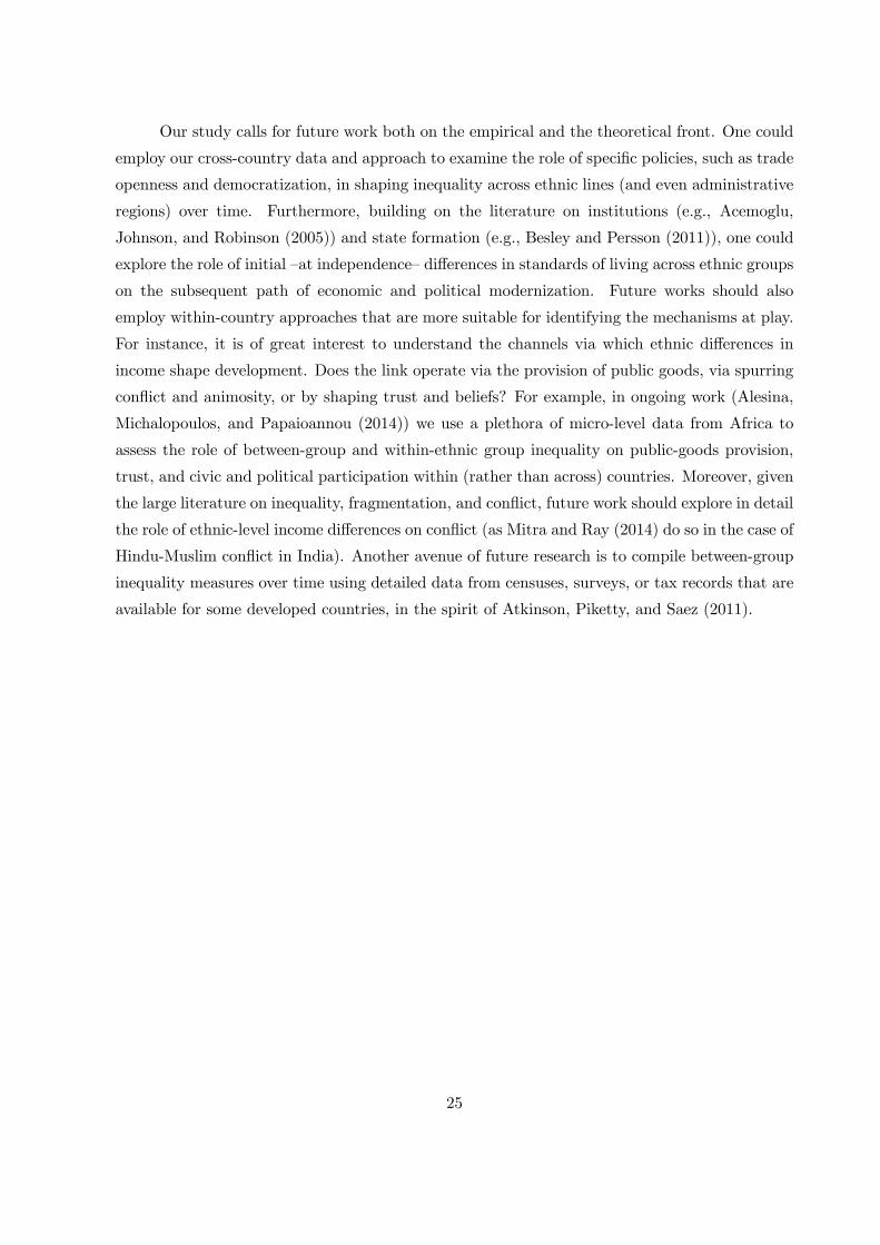
Our study calls for future work both on the empirical and the theoretical front. One could

employ our cross-country data and approach to examine the role of specific policies, such as trade

openness and democratization, in shaping inequality across ethnic lines (and even administrative

regions) over time. Furthermore, building on the literature on institutions (e.g., Acemoglu,

Johnson, and Robinson (2005)) and state formation (e.g., Besley and Persson (2011)), one could

explore the role of initial —at independence— differences in standards of living across ethnic groups

on the subsequent path of economic and political modernization. Future works should also

employ within-country approaches that are more suitable for identifying the mechanisms at play.

For instance, it is of great interest to understand the channels via which ethnic differences in

income shape development. Does the link operate via the provision of public goods, via spurring

conflict and animosity, or by shaping trust and beliefs? For example, in ongoing work (Alesina,

Michalopoulos, and Papaioannou (2014)) we use a plethora of micro-level data from Africa to

assess the role of between-group and within-ethnic group inequality on public-goods provision,

trust, and civic and political participation within (rather than across) countries. Moreover, given

the large literature on inequality, fragmentation, and conflict, future work should explore in detail

the role of ethnic-level income differences on conflict (as Mitra and Ray (2014) do so in the case of

Hindu-Muslim conflict in India). Another avenue of future research is to compile between-group

inequality measures over time using detailed data from censuses, surveys, or tax records that are

available for some developed countries, in the spirit of Atkinson, Piketty, and Saez (2011).

25

7 Maps & Figures

Figures 1 and 2 provide an illustration of the construction of the ethnic inequality measures for

Afghanistan. The Atlas Narodov Mira (GREG) maps 31 ethnicities (Figure 1a) whereas the

Ethnologue reports 39 languages (Figure 1b).

Ü

Ethnic Homelands in Afghanistan

Afghanistan Arabs

Afghans

Arabs of Middle Asia

Baloch

Brahui

Burushaskis

Firoz-Kohis

Hazara-Berberi

Hazara-Deh-i-Zainat

Ishkashimis

Jamshidis

Kazakhs

Kho

Kirghis

Mongols

Nuristanis

Ormuri

Pamir Tajiks

Parachi

Pashai

Persians

Roshanls

Russians

Shugnanis

Taimanis

Tajiks

Teymurs

Tirahi

Turkmens

Uzbeks

Yazghulems

Overlapping Languages

Ethnologue Languages in Afghanistan

Aimaq

Ashkun

Brahui

Darwazi

Eastern Farsi

Gawar-Bati

Grangali

Gujari

Hazaragi

Kamviri

Kati

Kirghiz

Malakhel

Mogholi

Munji

Northeast Pashayi

Northwest Pashayi

Ormuri

Pahlavani

Parya

Prasuni

Sanglechi-Ishkashimi

Savi

Shughni

Shumashti

Southeast Pashayi

Southern Pashto

Southern Uzbek

Southwest Pashayi

Tajiki Spoken Arabic

Tangshewi

Tirahi

Tregami

Turkmen

Waigali

Wakhi

Warduji

Western Balochi

Wotapuri-Katarqalai

Ü

Figure 1a Figure 1b

Figures 2a and 2b portray the distribution of lights per capita for each group based on

GREG and Ethnologue mapping with lighter colors indicating more brightly lit areas.

Figure 2a Figure 2b

Figure 3 illustrates the construction of the overall spatial inequality. When we divide the

globe into boxes of 25 x 25 decimal-degree boxes, we get 24 areas in Afghanistan.

26

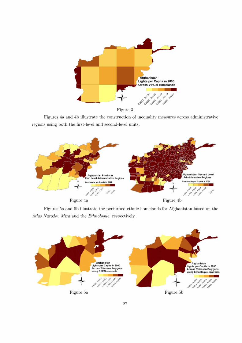
Ü

Afghanistan Lights per Capita in 2000Across Virtual Homelands

0.00

22 -

0.00

64

0.00

10 -

0.00

21

0.00

04 -

0.00

09

0.00

02 -

0.00

03

0.00

00 -

0.00

01

Figure 3

Figures 4a and 4b illustrate the construction of inequality measures across administrative

regions using both the first-level and second-level units.

Figure 4a Figure 4b

Figures 5a and 5b illustrate the perturbed ethnic homelands for Afghanistan based on the

Atlas Narodov Mira and the Ethnologue, respectively.

Figure 5a Figure 5b

27

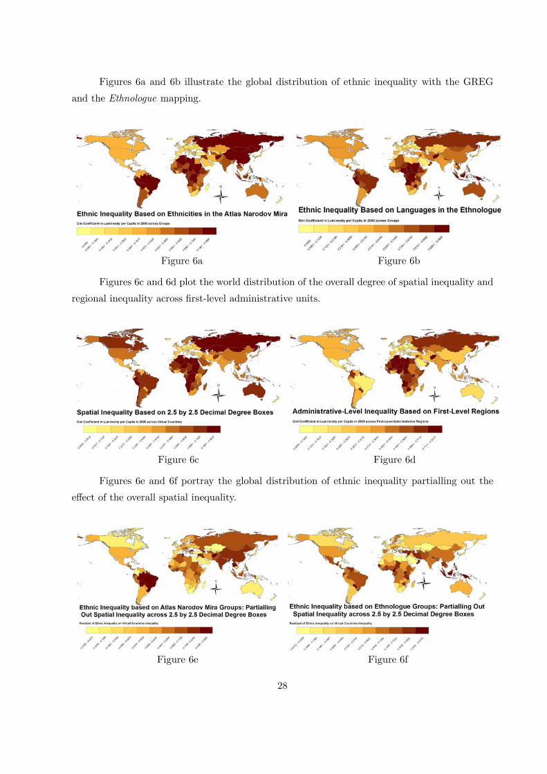
Figures 6a and 6b illustrate the global distribution of ethnic inequality with the GREG

and the Ethnologue mapping.

Figure 6a Figure 6b

Figures 6c and 6d plot the world distribution of the overall degree of spatial inequality and

regional inequality across first-level administrative units.

Figure 6c Figure 6d

Figures 6e and 6f portray the global distribution of ethnic inequality partialling out the

effect of the overall spatial inequality.

Figure 6e Figure 6f

28

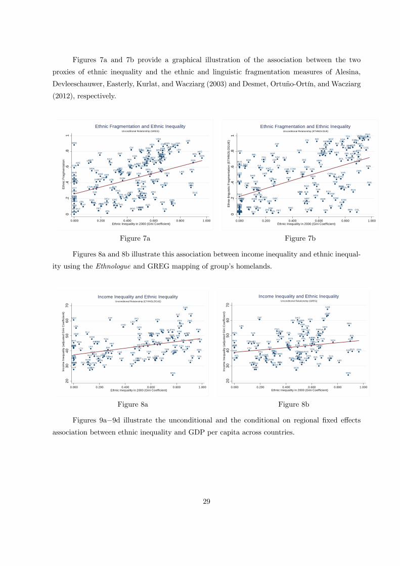
Figures 7a and 7b provide a graphical illustration of the association between the two

proxies of ethnic inequality and the ethnic and linguistic fragmentation measures of Alesina,

Devleeschauwer, Easterly, Kurlat, and Wacziarg (2003) and Desmet, Ortuño-Ortín, and Wacziarg

(2012), respectively.

AFGAGO

ALB

ARE

ARG

ARMATG

AUSAUT

AZE

BDI

BEL

BEN

BFA

BGD

BGR

BHR

BHS

BIH

BLR

BLZBOL

BRABRN

BTN

BWA

CAF

CAN

CHE

CHLCHN

CIV

CMR ZARCOG

COL

COM

CPV

CRI

CUB

CYP

CZE

DEU

DJI

DMA

DNK

DOM

DZA

ECU

EGY

ERI

ESP

EST

ETH

FIN

FJI

FRA

GAB

GBR

GEO

GHA

GIN

GMBGNB

GNQ

GRC

GRD

GTM

GUY

HND

HRV

HTI

HUN

IDN

IND

IRL

IRN

IRQ

ISL

ISR

ITA

JAM

JOR

JPN

KAZ

KEN

KGZ

KHMKNA

KOR

KWT

LAO

LBN

LBR

LBY

LCA

LKA

LSO

LTU

LUX

LVA

MAR

MDA

MDG

MEX

MKD

MLI

MLT

MNG

MOZ

MRT

MUS

MWI

MYS

NAMNER

NGA

NIC

NLD

NOR

NPL

NZL

OMN

PAK

PAN

PER

PHLPNG

POL

PRT

PRY

QAT

ROM

RUS

RWA

SAU

SDNSEN

SGP

SLB

SLE

SLV

SOM

SUR

SVKSVN

SWESWZ

SYC

SYR

TCD

TGO

THA

TJK

TKM

TON

TTO

TUN

TUR

TZA

UGA

UKR

URY

USA

UZB

VCT

VEN

VNM

VUT

WSM

ZAFZMB

ZWE

0.2

.4.6

.81

Eth

nic

Fra

gm

en

tatio

n

0.000 0.200 0.400 0.600 0.800 1.000Ethnic Inequality in 2000 (Gini Coefficient)

Unconditional Relationship (GREG)

Ethnic Fragmentation and Ethnic Inequality

AFG

AGO

ALB

ARE

ARGARM

ATG

AUS

AUT

AZE

BDI

BEL

BEN

BFA

BGD

BGR

BHR

BHSBIH

BLR

BLZ BOL

BRA

BRN

BTN

BWA

CAF

CANCHE

CHL

CHN

CIVCMRZAR

COG

COL

COM

CPVCRI

CUB

CYP

CZE

DEU

DJI

DMA

DNKDOM

DZA

ECU

EGY

ERI

ESPEST

ETH

FIN

FJI

FRA

GAB

GBR

GEO

GHA

GINGMB

GNB

GNQ

GRC

GRD

GTM

GUYHND

HRV

HTI

HUN

IDN

IND

IRL

IRN

IRQ

ISL

ISR

ITA

JAM

JOR

JPN

KAZ

KEN

KGZ

KHM

KNAKOR

KWT

LAO

LBN

LBR

LBY

LCA

LKA

LSO

LTU

LUX

LVA

MAR

MDA

MDG

MEX

MKD

MLI

MLT

MNG

MOZ

MRT

MUS

MWI

MYS

NAM

NER

NGA

NIC

NLD

NOR

NPL

NZL

OMN

PAK

PAN

PER

PHL

PNG

POLPRT

PRY

QAT

ROM

RUS

RWA

SAUSDN

SENSGP

SLB

SLE

SLV

SOM

SUR

SVK

SVN SWE

SWZ

SYC

SYR

TCD

TGO

THA

TJK

TKM

TON

TTO

TUN

TUR

TZAUGA

UKR

URY

USA

UZB

VCTVEN

VNM

VUT

WSM

ZAF ZMB

ZWE

0.2

.4.6

.81

Eth

no

-lin

gu

istic

Fra

gm

en

tatio

n (

ET

HN

OL

OG

UE

)

0.000 0.200 0.400 0.600 0.800 1.000Ethnic Inequality in 2000 (Gini Coefficient)

Unconditional Relationship (ETHNOLOUE)

Ethnic Fragmentation and Ethnic Inequality

Figure 7a Figure 7b

Figures 8a and 8b illustrate this association between income inequality and ethnic inequal-

ity using the Ethnologue and GREG mapping of group’s homelands.

ARG

ARM

AUS

AUT

AZE

BDI

BEL

BFA

BGD

BGR

BHS

BIH

BLR

BOL

BRA

BWA

CAF

CAN

CHE

CHL

CHN

CIV

COL

CRI

CZE

DEUDNK

DOM

DZA

ECU

EGYESP

EST ETH

FIN

FJI

FRA

GAB

GBR

GEO

GHA

GINGMB

GRC

GTM

GUY

HND

HUN

IDNIND

IRL

IRQ

ISR

ITA

JAMJOR

JPN

KAZ

KEN

KGZ

KHM

KORLAO

LBN

LKA

LSO

LTU

LUX

LVA

MDA

MDGMEX

MKD

MLI

MNG

MRTMUS

MYS

NER

NGA

NIC

NLDNOR

NPL

NZLPAK

PAN

PERPHL

PNG

POL

PRT

PRY

ROM

RUS

RWA

SDN

SEN

SGP

SLE

SLV

SUR

SVK

SVN

SWE

SWZ

TCD

THA

TKM

TTOTUN

TUR

TZA

UGA

UKR

URY

USA

VEN

VNM

ZAF

ZMB

ZWE

20

30

40

50

60

70

Inco

me

In

equ

alit

y (a

dju

ste

d G

ini C

oe

ffic

ien

t)

0.000 0.200 0.400 0.600 0.800 1.000Ethnic Inequality in 2000 (Gini Coefficient)

Unconditional Relationship (ETHNOLOGUE)

Income Inequality and Ethnic Inequality

ARG

ARM

AUS

AUT

AZE

BDI

BEL

BFA

BGD

BGR

BHS

BIH

BLR

BOL

BRA

BWA

CAF

CAN

CHE

CHL

CHN

CIV

COL

CRI

CZE

DEUDNK

DOM

DZA

ECU

EGYESP

EST ETH

FIN

FJI

FRA

GAB

GBR

GEO

GHA

GINGMB

GRC

GTM

GUY

HND

HUN

IDNIND

IRL

IRQ

ISR

ITA

JAMJOR

JPN

KAZ

KEN

KGZ

KHM

KORLAO

LBN

LKA

LSO

LTU

LUX

LVA

MDA

MDG MEX

MKD

MLI

MNG

MRTMUS

MYS

NER

NGA

NIC

NLDNOR

NPL

NZLPAK

PAN

PERPHL

PNG

POL

PRT

PRY

ROM

RUS

RWA

SDN

SEN

SGP

SLE

SLV

SUR

SVK

SVN

SWE

SWZ

TCD

THA

TKM

TTOTUN

TUR

TZA

UGA

UKR

URY

USA

VEN

VNM

ZAF

ZMB

ZWE

20

30

40

50

60

70

Inco

me

In

equ

alit

y (a

dju

ste

d G

ini C

oe

ffic

ien

t)

0.000 0.200 0.400 0.600 0.800 1.000Ethnic Inequality in 2000 (Gini Coefficient)

Unconditional Relationship (GREG)

Income Inequality and Ethnic Inequality

Figure 8a Figure 8b

Figures 9a−9d illustrate the unconditional and the conditional on regional fixed effectsassociation between ethnic inequality and GDP per capita across countries.

29

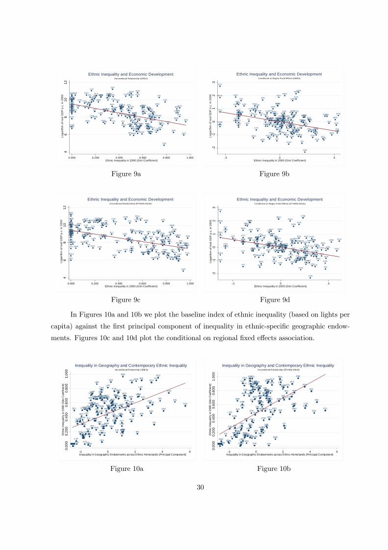
AFG

AGO

ALB

ARE

ARG

ARM

ATG

AUSAUT

AZE

BDI

BEL

BEN

BFABGD

BGR

BHRBHS

BIHBLRBLZ

BOL

BRA

BRN

BTN

BWA

CAF

CANCHE

CHL

CHN

CIV CMR

ZAR

COG

COL

COM

CPV

CRICUB

CYP CZE

DEU

DJI

DMA

DNK

DOM

DZAECUEGY

ERI

ESP

EST

ETH

FIN

FJI

FRA

GAB

GBR

GEO

GHAGINGMB

GNB

GNQ

GRC

GRD

GTM

GUYHND

HRV

HTI

HUN

IDN

IND

IRL

IRN

IRQ

ISL

ISRITA

JAM

JOR

JPN

KAZ

KEN

KGZ

KHM

KNA

KOR

KWT

LAO

LBN

LBR

LBY

LCA

LKA

LSO

LTU

LUX

LVA

MAR

MDA

MDG

MEX

MKD

MLI

MLT

MNG

MOZ

MRT

MUS

MWI

MYS

NAM

NER

NGA

NIC

NLDNOR

NPL

NZLOMN

PAK

PAN

PER

PHLPNG

POL

PRT

PRY

QAT

ROM

RUS

RWA

SAU

SDNSEN

SGP

SLB

SLE

SLV

SOM

SUR

SVK

SVN

SWE

SWZ

SYC

SYR

TCDTGO

THA

TJK

TKM

TON

TTO

TUN

TUR

TZAUGA

UKR

URY

USA

UZB

VCT

VEN

VNM

VUTWSM ZAF

ZMB

ZWE

46

81

01

2L

og

ari

thm

of

rea

l GD

P p

.c.

in 2

00

0

0.000 0.200 0.400 0.600 0.800 1.000Ethnic Inequality in 2000 (Gini Coefficient)

Unconditional Relationship (GREG)

Ethnic Inequality and Economic Development

AFG

AGO

ALB

ARE

ARG

ARM

ATG

AUS

AUT

AZE

BDI

BELBEN

BFABGD

BGR

BHR

BHS

BIHBLR BLZ

BOL

BRA

BRN

BTN

BWA

CAF

CAN

CHE

CHL

CHN

CIVCMR

ZAR

COG

COLCOM

CPV

CRICUB

CYP

CZE

DEU

DJI

DMA

DNKDOM

DZA

ECU

EGY

ERIESP

EST

ETH

FIN

FJI

FRA

GAB

GBR

GEO

GHAGINGMB

GNB

GNQ

GRCGRD

GTM

GUYHND

HRV

HTI

HUN

IDN

IND

IRL

IRN

IRQ

ISL

ISR

ITA

JAM

JOR

JPN

KAZKEN

KGZ

KHM

KNA

KOR KWT

LAO

LBN

LBR

LBYLCA

LKA

LSO

LTULUX

LVA

MAR

MDA

MDG

MEX

MKD

MLI

MLT

MNGMOZ

MRT

MUS

MWI

MYS

NAM

NER

NGA

NIC

NLDNOR

NPL

NZL

OMNPAK

PAN

PER

PHLPNG

POL

PRT

PRY

QAT

ROM

RUS

RWA

SAU SDN

SEN

SGP

SLB

SLE

SLV

SOM

SUR

SVK

SVN

SWE

SWZ

SYC

SYR

TCDTGO

THA

TJK

TKM

TON

TTO

TUN

TUR

TZAUGAUKR

URYUSA

UZB

VCT

VEN

VNM

VUTWSM

ZAF

ZMB

ZWE

-2-1

01

23

Lo

ga

rith

m o

f re

al G

DP

p.c

. in

20

00

-.5 0 .5Ethnic Inequality in 2000 (Gini Coefficient)

Conditional on Region Fixed Effects (GREG)

Ethnic Inequality and Economic Development

Figure 9a Figure 9b

AFG

AGO

ALB

ARE

ARG

ARM

ATG

AUSAUT

AZE

BDI

BEL

BEN

BFABGD

BGR

BHRBHS

BIHBLRBLZ

BOL

BRA

BRN

BTN

BWA

CAF

CANCHE

CHL

CHN

CIV CMR

ZAR

COG

COL

COM

CPV

CRICUB

CYP CZE

DEU

DJI

DMA

DNK

DOM

DZAECUEGY

ERI

ESP

EST

ETH

FIN

FJI

FRA

GAB

GBR

GEO

GHAGINGMB

GNB

GNQ

GRC

GRD

GTM

GUYHND

HRV

HTI

HUN

IDN

IND

IRL

IRN

IRQ

ISL

ISRITA

JAM

JOR

JPN

KAZ

KEN

KGZ

KHM

KNA

KOR

KWT

LAO

LBN

LBR

LBY

LCA

LKA

LSO

LTU

LUX

LVA

MAR

MDA

MDG

MEX

MKD

MLI

MLT

MNG

MOZ

MRT

MUS

MWI

MYS

NAM

NER

NGA

NIC

NLDNOR

NPL

NZLOMN

PAK

PAN

PER

PHL PNG

POL

PRT

PRY

QAT

ROM

RUS

RWA

SAU

SDNSEN

SGP

SLB

SLE

SLV

SOM

SUR

SVK

SVN

SWE

SWZ

SYC

SYR

TCDTGO

THA

TJK

TKM

TON

TTO

TUN

TUR

TZAUGA

UKR

URY

USA

UZB

VCT

VEN

VNM

VUTWSM ZAF

ZMB

ZWE

46

81

01

2L

og

ari

thm

of

rea

l GD

P p

.c.

in 2

00

0

0.000 0.200 0.400 0.600 0.800 1.000Ethnic Inequality in 2000 (Gini Coefficient)

Unconditional Relationship (ETHNOLOGUE)

Ethnic Inequality and Economic Development

AFG

AGO

ALB

ARE

ARG

ARM

ATG

AUS

AUT

AZE

BDI

BEL BEN

BFABGD

BGR

BHR

BHS

BIHBLR BLZ

BOL

BRA

BRN

BTN

BWA

CAF

CANCHE

CHL

CHN

CIVCMR

ZAR

COG

COLCOM

CPV

CRICUB

CYP

CZE

DEU

DJI

DMA

DNKDOM

DZA

ECU

EGY

ERIESP

EST

ETH

FIN

FJI

FRA

GAB

GBR

GEO

GHAGINGMB

GNB

GNQ

GRCGRD

GTM

GUYHND

HRV

HTI

HUN

IDN

IND

IRL

IRN

IRQ

ISL

ISR

ITA

JAM

JOR

JPN

KAZKEN

KGZ

KHM

KNA

KOR KWT

LAO

LBN

LBR

LBYLCA

LKA

LSO

LTULUX

LVA

MAR

MDA

MDG

MEX

MKD

MLI

MLT

MNGMOZ

MRT

MUS

MWI

MYS

NAM

NER

NGA

NIC

NLDNOR

NPL

NZL

OMNPAK

PAN

PER

PHLPNG

POL

PRT

PRY

QAT

ROM

RUS

RWA

SAU SDN

SEN

SGP

SLB

SLE

SLV

SOM

SUR

SVK

SVN

SWE

SWZ

SYC

SYR

TCDTGO

THA

TJK

TKM

TON

TTO

TUN

TUR

TZAUGAUKR

URYUSA

UZB

VCT

VEN

VNM

VUTWSM

ZAF

ZMB

ZWE

-2-1

01

23

Lo

ga

rith

m o

f re

al G

DP

p.c

. in

20

00

-.5 0 .5Ethnic Inequality in 2000 (Gini Coefficient)

Conditional on Region Fixed Effects (ETHNOLOGUE)

Ethnic Inequality and Economic Development

Figure 9c Figure 9d

In Figures 10a and 10b we plot the baseline index of ethnic inequality (based on lights per

capita) against the first principal component of inequality in ethnic-specific geographic endow-

ments. Figures 10c and 10d plot the conditional on regional fixed effects association.

AFG

AGO

ALB

ARE

ARG

ARM

AUS

AUT

AZEBDI

BEL

BEN BFA

BGDBGR

BHRBHS

BIHBLR

BLZ

BOLBRA

BRN

BTN

BWA

CAF

CAN

CHE

CHL

CHN

CIV

CMR

ZAR

COG

COL

COMCPV

CRI

CUB

CYP

CZE

DEU

DJI

DNK

DOM

DZA

ECU

EGYERI

ESP

EST

ETH

FIN

FJI

FRA

GAB

GBR

GEO

GHA

GIN

GMB

GNB GNQ

GRC

GTM

GUY HND

HRV

HTI

HUN

IDN

IND

IRL

IRN

IRQ

ISL

ISR

ITA

JAM

JOR

JPN

KAZ

KEN

KGZ

KHM

KOR

KWT

LAO

LBN

LBR

LBY

LKA

LSO

LTU

LUX

LVA

MAR

MDA

MDG

MEXMKD

MLI

MNG

MOZ

MRT

MUS

MWI

MYS

NAM

NER

NGA

NIC

NLD

NOR

NPL

NZL

OMN

PAK

PAN

PER

PHL

PNG

POLPRT

PRY

QAT

ROM

RUS

RWA

SAU

SDN

SEN

SGP

SLBSLE

SLV

SOM

SUR

SVK

SVN

SWESWZ

SYR

TCD

TGO

THATJK

TKM

TTO

TUN

TUR

TZA

UGA

UKR

URY

USA

UZB

VEN

VNM

VUTWSM

ZAF

ZMB

ZWE

0.0

00

0.2

00

0.4

00

0.6

00

0.8

00

1.0

00

Eth

nic

Ineq

ualit

y in

200

0 (

Gin

i Coe

ffic

ient

)

-2 0 2 4 6Inequality in Geographic Endowments across Ethnic Homelands (Principal Component)

Unc onditional Relationship ( GRE G)

Inequality in Geography and Contemporary Ethnic Inequality

AFGAGO

ALB

ARE

ARG

ARM

AUS

AUT

AZE

BDI

BEL

BEN

BFA

BGD

BGR

BHR

BHS

BIH

BLR

BLZ

BOL

BRA

BRN

BTN

BWA

CAF

CAN

CHE

CHL

CHN

CIV

CMRZARCOG

COL

COM

CPV

CRI

CUB

CYP

CZE

DEUDJI

DNK

DOM

DZA

ECU

EGY

ERI

ESP

EST

ETH

FIN

FJI

FRA

GAB

GBR

GEO

GHA

GIN

GMB

GNB

GNQ

GRC

GTM

GUY

HND

HRVHTI

HUN

IDN

IND

IRL

IRN

IRQ

ISL

ISRITA

JAM

JOR

JPN

KAZ

KEN

KGZ

KHM

KOR

KWT

LAO

LBN

LBR

LBY

LKA

LSO

LTU

LUX LVA

MAR

MDA

MDG

MEX

MKD

MLIMNG

MOZ

MRT

MUS

MWI

MYS

NAM

NERNGA

NIC

NLD

NOR

NPL

NZL

OMN

PAK

PAN

PER

PHL

PNG

POL

PRT

PRY

QAT

ROM

RUS

RWASAU

SDN

SEN

SGP

SLB

SLE

SLV

SOM

SUR

SVK

SVN

SWE

SWZ

SYR

TCD

TGO

THA

TJKTKM

TTO

TUN

TUR

TZAUGA

UKR

URY

USA

UZB

VEN

VNM

VUT

WSM

ZAF

ZMB

ZWE

0.0

00

0.2

00

0.4

00

0.6

00

0.8

00

1.0

00

Eth

nic

Ineq

ualit

y in

200

0 (

Gin

i Coe

ffic

ient

)

-2 0 2 4 6Inequality in Geographic Endowments across Ethnic Homelands (Principal Component)

Unconditional Relationship ( ETHNOLOGUE)

Inequality in Geography and Contemporary Ethnic Inequality

Figure 10a Figure 10b

30

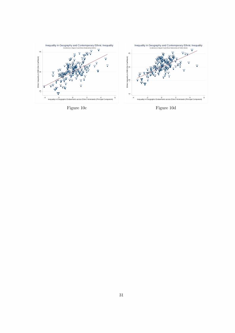
AFG

AGO

ALB

ARE

ARG

ARM

AUS

AUT

AZE

BDI

BELBENBFA

BGD

BGR

BHR

BHS

BIHBLR

BLZ

BOLBRA

BRN

BTN

BWA

CAF

CAN

CHE

CHL

CHN

CIV

CMR

ZAR

COG

COL

COMCPV

CRI

CUB

CYP CZE

DEUDJI

DNK

DOM

DZA

ECU EGY

ERI

ESP

EST

ETH

FIN

FJI FRA

GAB

GBR

GEO

GHA

GIN

GMB

GNB GNQ

GRCGTM

GUY HND

HRV

HTI

HUN

IDN

IND

IRL

IRN

IRQ

ISL

ISR

ITA

JAM

JOR

JPN

KAZ

KEN

KGZ

KHM

KOR

KWT

LAO

LBN

LBR

LBY

LKA

LSO

LTU

LUX

LVA

MAR

MDA

MDG

MEX

MKD

MLI

MNG

MOZ

MRT

MUS

MWIMYS

NAM

NER

NGA

NIC

NLD

NOR

NPL

NZL

OMN

PAK

PAN

PER

PHL

PNG

POLPRT

PRYQAT

ROM

RUS

RWA

SAU

SDN

SEN

SGP

SLB

SLE

SLV

SOM

SUR

SVK

SVN

SWE

SWZ

SYR

TCD

TGO

THATJK

TKM

TTO

TUN

TUR

TZA

UGA

UKR

URY

USA

UZBVEN

VNM

VUTWSM

ZAF

ZMBZWE

-.5

0.5

Eth

nic

Ineq

ualit

y in

200

0 (

Gin

i Coe

ffic

ient

)

-4 -2 0 2 4 6Inequality in Geographic Endowments across Ethnic Homelands (Principal Component)

Condi tional on Region Fixed Effects Relationsh ip (GREG)

Inequality in Geography and Contemporary Ethnic Inequality

AFGAGOALB

ARE

ARG

ARM

AUS

AUT

AZE

BDI

BEL

BEN

BFA

BGD BGR

BHR

BHS

BIH

BLR

BLZ

BOL

BRA

BRN

BTN

BWA

CAF

CAN

CHE

CHLCHN

CIV

CMRZARCOG

COL

COM

CPV

CRI

CUB

CYPCZE

DEU

DJI

DNK

DOM

DZA

ECUEGY

ERI

ESP

EST

ETHFIN

FJI

FRA

GAB

GBR

GEO

GHA

GIN

GMB

GNB

GNQ

GRC

GTMGUY

HND

HRV

HTI

HUN

IDN

INDIRL

IRN

IRQ

ISL

ISR

ITA

JAM

JOR

JPN

KAZKEN

KGZ

KHM

KOR

KWT

LAO

LBN

LBR

LBY

LKA

LSOLTULUX LVA MAR

MDA

MDG

MEX

MKD

MLI

MNG

MOZ

MRT

MUS

MWI

MYS

NAM

NERNGANIC

NLD

NORNPL

NZL

OMN

PAK

PAN

PER

PHL

PNG

POL

PRT

PRY

QAT

ROM

RUS

RWA

SAU

SDN

SEN

SGP

SLB

SLE

SLV

SOM

SUR

SVK

SVN

SWE

SWZ

SYR

TCD

TGO

THA

TJKTKM

TTO

TUN

TUR

TZAUGA

UKR

URY

USA UZB

VEN

VNM

VUT

WSM

ZAF

ZMB

ZWE

-1-.

50

.5E

thni

c In

equa

lity

in 2

000

(G

ini C

oeff

icie

nt)

-4 -2 0 2 4 6Inequality in Geographic Endowments across Ethnic Homelands (Principal Component)

Condi tional on Region Fixed Effects Relationsh ip (ETHNOLOGUE)

Inequality in Geography and Contemporary Ethnic Inequality

Figure 10c Figure 10d

31

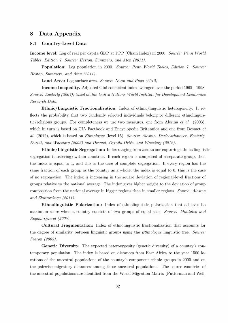
8 Data Appendix

8.1 Country-Level Data

Income level: Log of real per capita GDP at PPP (Chain Index) in 2000. Source: Penn World

Tables, Edition 7. Source: Heston, Summers, and Aten (2011).

Population: Log population in 2000. Source: Penn World Tables, Edition 7. Source:

Heston, Summers, and Aten (2011).

Land Area: Log surface area. Source: Nunn and Puga (2012).

Income Inequality. Adjusted Gini coefficient index averaged over the period 1965−1998.Source: Easterly (2007); based on the United Nations World Institute for Development Economics

Research Data.

Ethnic/Linguistic Fractionalization: Index of ethnic/linguistic heterogeneity. It re-

flects the probability that two randomly selected individuals belong to different ethnolinguis-

tic/religious groups. For completeness we use two measures, one from Alesina et al. (2003),

which in turn is based on CIA Factbook and Encyclopedia Britannica and one from Desmet et

al. (2012), which is based on Ethnologue (level 15). Source: Alesina, Devleeschauwer, Easterly,

Kurlat, and Wacziarg (2003) and Desmet, Ortuño-Ortín, and Wacziarg (2012).

Ethnic/Linguistic Segregation: Index ranging from zero to one capturing ethnic/linguistic

segregation (clustering) within countries. If each region is comprised of a separate group, then

the index is equal to 1, and this is the case of complete segregation. If every region has the

same fraction of each group as the country as a whole, the index is equal to 0; this is the case

of no segregation. The index is increasing in the square deviation of regional-level fractions of

groups relative to the national average. The index gives higher weight to the deviation of group

composition from the national average in bigger regions than in smaller regions. Source: Alesina

and Zhuravskaya (2011).

Ethnolinguistic Polarization: Index of ethnolinguistic polarization that achieves its

maximum score when a country consists of two groups of equal size. Source: Montalvo and

Reynal-Querol (2005).

Cultural Fragmentation: Index of ethnolinguistic fractionalization that accounts for

the degree of similarity between linguistic groups using the Ethnologue linguistic tree. Source:

Fearon (2003).

Genetic Diversity. The expected heterozygosity (genetic diversity) of a country’s con-

temporary population. The index is based on distances from East Africa to the year 1500 lo-

cations of the ancestral populations of the country’s component ethnic groups in 2000 and on

the pairwise migratory distances among these ancestral populations. The source countries of

the ancestral populations are identified from the World Migration Matrix (Putterman and Weil,

32

2010), and the modern capital cities of these countries are used to compute the aforementioned

migratory distances. The measure of genetic diversity is then computed by applying (i) the coef-

ficients obtained from regressing expected heterozygosity on migratory distance from East Africa

at the ethnic group level, using a worldwide sample of 53 ethnic groups comprising the Human

Genome Diversity Cell Line Panel, compiled by the Human Genome Diversity Project (HGDP)

and the Centre d’Étude du Polymorphisme Humain (CEPH); (ii) the coefficients obtained from

regressing pairwise genetic distance on pairwise migratory distance in a sample of 1 378 HGDP-

CEPH ethnic group pairs, and (iii) the ancestry weights representing the fractions of the year

2000 national population that can trace their ancestral origins to different source countries in the

year 1500. Source: Ashraf and Galor (2013).

Soil Quality: Percentage of each country with fertile soil. Source: Nunn and Puga (2012).

Ruggedness: The terrain ruggedness index quantifies topographic heterogeneity. The

index is the average across all grid cells in the country not covered by water. The units for the

terrain ruggedness index correspond to the units used to measure elevation differences. Rugged-

ness is measured in hundreds of metres of elevation difference for grid points 30 arc-seconds (926

metres on the equator or any meridian) apart. Source: Nunn and Puga (2012).

Tropical: The percentage of the land surface of each country with tropical climate. Source:

Nunn and Puga (2012).

Gem-Quality Diamond Extraction: Carats of gem-quality diamond extraction be-

tween 1958 and 2000, normalized by land area. Source: Nunn and Puga (2012).

Common Law: Indicator variable that identifies countries that have a common law legal

system. Source: La Porta, Lopez-de-Silanes, Shleifer, and Vishny (1999) and Nunn and Puga

(2012).

European Descent: The variable, calculated from version 11 of the migration matrix

of Putterman and Weil (2010), estimates the percentage of the year 2000 population in every

country that is descended from people who resided in Europe in 1500. Source: Nunn and Puga

(2012).

Settler Mortality: Log of mortality rates faced by European colonizers in late 19th

century. Source: Acemoglu, Johnson, and Robinson (2001).

Population Density before Colonization: Log of population density around 1500 CE.

Source: Acemoglu, Johnson, and Robinson (2002) and Nunn and Puga (2012).

Border Straightness Index: The 0 − 1 index reflects how straight —and thus likely tobe non-organic— national borders are. Source: Alesina, Easterly, and Matuszeski (2011).

Neolithic Transition: The logarithm of the number of thousand years elapsed (as of

the year 2000) since the majority of the population residing within a countries modern national

33

borders began practicing sedentary agriculture as the primary mode of subsistence. This measure,

reported by Putterman (2008), is compiled using a wide variety of both region- and country-

specific archaeological studies as well as more general encyclopedic works on the transition from

hunting and gathering to agriculture during the Neolithic Revolution Source: Ashraf and Galor

(2013) and Putterman and Weil (2010).

Ethnic Partitioning: Percentage of the population of a country that belongs to parti-

tioned ethnic groups. Source: Alesina, Easterly, and Matuszeski (2011).

Regional Fixed Effects: The region constants correspond to: South-East Asia and the

Pacific, Latin America and the Caribbean, North America, Western Europe, Eastern Europe and

Central Asia, the Middle East and Northern Africa, and Sub-Saharan Africa. The classification

follows World Bank’s World Development Indicators Database.

8.2 Group-Level Data

Light Density at Night per Capita: Light density is calculated by averaging luminosity ob-

servations across pixels that fall within each territory (ethnic/linguistic homelands, boxes of 25

x 25 decimal degrees, administrative units, and Thiessen polygons) and then dividing by popu-

lation density. Source: National Oceanic and Atmospheric Administration, National Geophysical

Data Center.

http://ngdc.noaa.gov/eog/dmsp/downloadV4composites.html.

Population Density: Average number of people per square kilometer for 1990 and 2000.

Source: Center for International Earth Science Information Network (CIESIN), Columbia Uni-

versity, and Centro Internacional de Agricultura Tropical (CIAT), 2005. Gridded Population of

the World Version 3 (GPWv3): Population Density Grids. Palisades, NY: Socioeconomic Data

and Applications Center (SEDAC), Columbia University.

http://sedac.ciesin.columbia.edu/gpw.

Area: Total area (in square kilometers) of each territory (ethnic/linguistic homelands,

boxes of 25 x 25 decimal degrees, administrative units, and Thiessen polygons).

Elevation: Average elevation above country minimum value in meters. Source: World-

Clim - Global Climate Data. Data were originally collected by NASA-JPL SRTM.

http://www.worldclim.org/current.

Land Suitability for Agriculture: Average land quality for cultivation within each

country. The index is the product of two components capturing the climatic and soil suitability

for farming. Source: Michalopoulos (2012); Original Source: Atlas of the Biosphere.

http://www.sage.wisc.edu/iamdata/grid_data_sel.php.

Distance to the Sea Coast: The geodesic distance from the centroid of each country

34

to the nearest coastline, measured in 1000s of kilometers. Source: Global Mapping International,

Colorado Springs, Colorado, USA. Series name: Global Ministry Mapping System. Series issue:

Version 3.0

Average Annual Precipitation: Average annual precipitation (mm) for the approxi-

mate 1950− 2000 time frame within the respective territory (ethnic/linguistic homelands, boxesof 25 x 25 decimal degrees, administrative units, and Thiessen polygons). Source: WorldClim -

Global Climate Data. http://www.worldclim.org/bioclim.

Average Annual Temperature: Average annual temperature for the approximate 1950−2000 time frame within the respective territory (ethnic/linguistic homelands, boxes of 25 x 25

decimal degrees, administrative units, and Thiessen polygons).

Source: WorldClim - Global Climate Data. http://www.worldclim.org/bioclim.

Precipitation Seasonality: Coefficient of variation of annual precipitation for the ap-

proximate 1950 − 2000 time frame within the respective territory (ethnic/linguistic homelands,boxes of 25 x 25 decimal degrees, administrative units, and Thiessen polygons). Source: World-

Clim - Global Climate Data. http://www.worldclim.org/bioclim.

Temperature Range: Range (estimated as the difference of the maximum value of the

warmest month minus the minimum value of the coldest month) of annual temperature for ap-

proximately the period 1950− 2000 within the respective territory (ethnic/linguistic homelands,boxes of 25 x 25 decimal degrees, administrative units, and Thiessen polygons). Source: World-

Clim - Global Climate Data. http://www.worldclim.org/bioclim.

35

References

Acemoglu, D., S. Johnson, and J. A. Robinson (2001): “The Colonial Origins of Compara-

tive Development: An Empirical Investigation,” American Economic Review, 91(5), 1369—1401.

(2002): “Reversal of Fortune: Geography and Institutions in the Making of the Modern

World Income Distribution,” Quarterly Journal of Economics, 107(4), 1231—1294.

(2005): “Institutions as a Fundamental Cause of Long-Run Growth,” in Handbook of

Economic Growth, ed. by P. Aghion, and S. N. Durlauf, pp. 109—139. Elsevier North-Holland,

Amsterdam, The Netherlands.

Acemoglu, D., S. Johnson, J. A. Robinson, and P. Yared (2008): “Income and Democ-

racy,” American Economic Review, 98(3), 808—842.

Alesina, A., A. Devleeschauwer, W. Easterly, S. Kurlat, and R. Wacziarg (2003):

“Fractionalization,” Journal of Economic Growth, 8(2), 155—194.

Alesina, A., W. Easterly, and J. Matuszeski (2011): “Artificial States,” Journal of the

European Economic Association, 9(2), 246—277.

Alesina, A., and E. L. Ferrara (2005): “Ethnic Diversity and Economic Performance,”

Journal of Economic Literature, 43, 762—800.

Alesina, A., J. Harnoss, and H. Rapoport (2013): “Birthplace Diversity and Economic

Prosperity,” NBER Working Paper, No. 18699.

Alesina, A., and E. Zhuravskaya (2011): “Segregation and the Quality of Government in a

Cross-Section of Countries,” American Economic Review, 101(5), 1872—1911.

Alesina, A. F., S. Michalopoulos, and E. Papaioannou (2014): “Inequality in Africa,”

mimeo, Brown, Harvard and LBS.

Anderson, S. (2011): “Caste as an Impediment to Trade,” American Economic Journal: Ap-

plied Economics, 3(1), 239—263.

Ashraf, Q., and O. Galor (2013): “The Out of Africa Hypothesis, Human Genetic Diversity,

and Comparative Economic Development,” American Economic Review, 103(1), 1—46.

Atkinson, A. B., T. Piketty, and E. Saez (2011): “Top Incomes in the Long Run of History,”

Journal of Economic Perspectives, 49(1), 3—71.

36

Baldwin, K., and J. D. Huber (2010): “Economic versus Cultural Differences: Forms of

Ethnic Diversity and Public Goods Provision,” American Political Science Review, 104(4),

644—662.

Benabou, R. (2005): “Inequality, Technology, and the Social Contract,” in Handbook of Eco-

nomic Growth, ed. by P. Aghion, and S. Durlauf, vol. 1, chap. 25, pp. 1595—1638. Elsevier,

North-Holland, Netherlands.

Besley, T., and T. Persson (2011): Pillars of Prosperity. The Political Economics of Devel-

opment Clusters. Princeton University Press, Princeton, NJ.

Bockstette, V., A. Chanda, and L. Putterman (2002): “States and Markets: The Advan-

tage of an Early Start,” Journal of Economic Growth, 7(4), 347—369.

Cederman, L.-E., N. B. Weidman, and K. S. Gleditch (2011): “Horizontal Inequalities

and Ethnonationalist Civil War: A Global Comparison,” American Political Science Review,

105(1), 478—495.

Chen, X., and W. D. Nordhaus (2011): “Using Luminosity Data as a Proxy for Economic

Statistics,” Proceeedings of the National Academy of Sciences, 108(21), 8589—8594.

Chua, A. (2003): World on Fire: How Exporting Free-Market Democracy Breds Ethnic Hatred

and Global Instability. William Heinemann, London, UK.

Deshpande, A. (2000): “Does Caste Still Define Disparity? A Look at Inequality in Kerala,

India,” American Economic Review, Papers and Proceedings, 90(2), 322—325.

Desmet, K., I. Ortuño-Ortín, and R. Wacziarg (2012): “The Political Economy of Ethno-

linguistic Cleavages,” Journal of Development Economics, 97(2), 322—338.

Diamond, J. (1997): Guns, Germs, and Steel. The Fates of Human Societies. W.W. Norton and

Co, New York, NY.

Easterly, W. (2007): “Inequality Does Cause Underdevelopment,” Journal of Development

Economics, 84(2), 755—776.

Esteban, J., L. Mayoral, and D. Ray (2012): “Ethnicity and Conflict: An Empirical Study,”

American Economic Review, 102(4), 1310—1342.

Esteban, J., and D. Ray (2011): “Linking Conflict to Inequality and Polarization,” American

Economic Review, 101(4), 1345—1374.

37

Ezcurra, R. (2013): “Does Economic Globalization affect Regional Inequality? A Cross-country

Analysis,” World Development, 52, 92—103.

Fearon, J. D. (2003): “Ethnic Structure and Cultural Diversity by Country,” Journal of Eco-

nomic Growth, 8, 195—222.

Galor, O. (2011): “Inequality, Human Capital and the Process of Development,” in Handbook

of the Economics of Education, ed. by S. M. Eric A. Hanushek, and L. Woessmann. Elsevier,

Amesterdam, Holland.

Gordon, R. G. (2005): “Ethnologue: Languages of the World,” .

Hall, R. E., and C. I. Jones (1999): “Why Do Some Countries Produce So Much More Output

Per Worker Than Others?,” Quarterly Journal of Economics, 114(1), 83—116.

Henderson, V. J., A. Storeygard, and D. N. Weil (2012): “Measuring Economic Growth

from Outer Space,” American Economic Review, 102(2), 994—1028.

Heston, A., R. Summers, and B. Aten (2011): “Penn World Table Version 7.0,” Center for

International Comparisons of Production, Income and Prices at the University of Pennsylvania.

Hodler, R., and P. A. Raschky (2014): “Regional Favoratism,” Quarterly Journal of Eco-

nomics, 129(2).

Horowitz, D. L. (1985): Ethnic Groups in Conflict. University of California Press, Berkeley

and Los Angeles, California.

Huber, J. D., and L. Mayoral (2013): “Inequality, Ethnicity and Civil Conflict,” Working

Paper, Department of Political Science, Columbia University.

Huber, J. D., and P. Suryanarayan (2013): “Ethnic Inequality and the Ethnification of Polit-

ical Parties: Evidence from India,” Working Paper, Department of Political Science, Columbia

University.

Kanbur, R., and A. J. Venables (2008): “Spatial Inequality and Development - Overview of

UNU-WIDER Project,” mimeo, Cornell University.

Kim, S. (2009): “SpatialaInequality and Economic Development: Theories, Facts, and Poli-

cies,” in Urbanization and Growth, ed. by P. A. Buckley R., and M. Spence, pp. 1—39. The

International Bank for Reconstruction and Development and World Bank.

Kyriacou, A. P. (2013): “Ethnic Group Inequalities and Governance: Evidence from Develop-

ing Countries,” Kyklos, 66(1), 78—101.

38

La Porta, R., F. Lopez-de-Silanes, A. Shleifer, and R. Vishny (1998): “Law and Fi-

nance,” Journal of Political Economy, 106(6), 1113—1155.

(1999): “The Quality of Government,” Journal of Law Economics and Organization,

15(1), 222—279.

Lessmann, C. (2014): “Spatial Inequality and Development U Is There an Inverted-U Relation-

ship?,” Journal of Development Economics, 106(3), 35—51.

Loury, G. C. (2002): The Anatomy of Racial Inequality. Harvard University Press, Cambridge,

MA.

Michalopoulos, S. (2012): “The Origins of Ethnolinguistic Diversity,” American Economic

Review, 102(4), 1508—1539.

Michalopoulos, S., and E. Papaioannou (2013): “Pre-colonial Ethnic Institutions and Con-

temporary African Development,” Econometrica, 81(1), 113—152.

(2014): “National Institutions and Subnational Development in Africa,” Quarterly

Journal of Economics, 129(1), 151—213.

Mitra, A., and D. Ray (2014): “Implications of an Economic Theory of Conflict: Hindu-

Muslim Violence in India,” Journal of Political Economy, 122, forthcoming.

Montalvo, J.-G., and M. Reynal-Querol (2005): “Ethnic Polarization, Potential Conflict,

and Civil Wars,” American Economic Review, 95(3), 796—816.

Nunn, N., and D. Puga (2012): “Ruggedness: The Blessing of Bad Geography in Africa,”

Review of Economics and Statistics, 94(1), 20—36.

Pinkovskiy, M. (2013): “Economic Discontinuities at Borders: Evidence from Satellite Data

on Lights at Night,” mimeo MIT.

Pinkovskiy, M., and X. Sala-i-Martin (2014): “Lights, Camera,... Income!: Estimating

Poverty Using National Accounts, Survey Means, and Lights,” NBER WP 19831.

Putterman, L., and D. N. Weil (2010): “Post-1500 Population Flows and the Long-Run

Determinants of Economic Growth and Inequality,” Quarterly Journal of Economics, 125(4),

1627—1682.

Robinson, J. A. (2001): “Social Identity, Inequality, and Conflict,” Economics of Governance,

2(2), 85—99.

39

Stewart, F. (2002): “Horizontal Inequalities: A Neglected Dimension of Development,” UNU

World Institute for Development Economics Research, Annual Lecture 5.

Tesei, A. (2014): “Trust, Racial Fragmentation, and Income Inequality: New Evidence from

the US,” mimeo, Queen Mary College, University of London.

Weidmann, N. B., J. K. Rod, and L.-E. Cederman (2010): “Representing Ethnic Groups

in Space: A New Dataset,” Journal of Peace Research, 47(4), 491—499.

Williamson, J. G. (1965): “Regional Inequality and the Process of National Development: A

Description of the Patterns,” Economic Development and Cultural Change, 13(4), 1—84.

Wooldridge, J. M. (2002): Econometric Analysis of Cross Section and Panel Data. MIT Press,

Cambridge, MA.

40

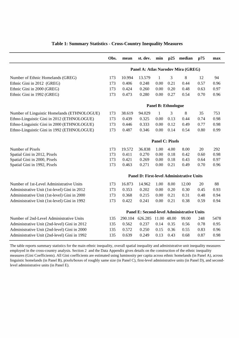
Obs. mean st. dev. min p25 median p75 max

Number of Ethnic Homelands (GREG) 173 10.994 13.579 1 3 8 12 94Ethnic Gini in 2012 (GREG) 173 0.406 0.248 0.00 0.21 0.44 0.57 0.96Ethnic Gini in 2000 (GREG) 173 0.424 0.260 0.00 0.20 0.48 0.63 0.97Ethnic Gini in 1992 (GREG) 173 0.473 0.280 0.00 0.27 0.54 0.70 0.96

Number of Linguistic Homelands (ETHNOLOGUE) 173 38.619 94.029 1 3 8 35 753Ethno-Linguistic Gini in 2012 (ETHNOLOGUE) 173 0.439 0.325 0.00 0.13 0.44 0.74 0.98Ethno-Linguistic Gini in 2000 (ETHNOLOGUE) 173 0.446 0.333 0.00 0.12 0.49 0.77 0.98Ethno-Linguistic Gini in 1992 (ETHNOLOGUE) 173 0.487 0.346 0.00 0.14 0.54 0.80 0.99

Number of Pixels 173 19.572 36.838 1.00 4.00 8.00 20 292Spatial Gini in 2012, Pixels 173 0.411 0.270 0.00 0.18 0.42 0.60 0.98Spatial Gini in 2000, Pixels 173 0.421 0.269 0.00 0.18 0.43 0.64 0.97Spatial Gini in 1992, Pixels 173 0.463 0.271 0.00 0.21 0.49 0.70 0.96

Number of 1st-Level Administrative Units 173 16.873 14.962 1.00 8.00 12.00 20 88Administrative Unit (1st-level) Gini in 2012 173 0.353 0.202 0.00 0.20 0.30 0.45 0.93Administrative Unit (1st-level) Gini in 2000 173 0.368 0.215 0.00 0.21 0.31 0.48 0.94Administrative Unit (1st-level) Gini in 1992 173 0.422 0.241 0.00 0.21 0.38 0.59 0.94

Number of 2nd-Level Administrative Units 135 290.104 626.285 11.00 48.00 99.00 248 5478Administrative Unit (2nd-level) Gini in 2012 135 0.562 0.237 0.14 0.35 0.56 0.78 0.95Administrative Unit (2nd-level) Gini in 2000 135 0.572 0.250 0.15 0.36 0.55 0.83 0.96Administrative Unit (2nd-level) Gini in 1992 135 0.639 0.249 0.13 0.43 0.68 0.87 0.98

Table 1: Summary Statistics - Cross-Country Inequality Measures

The table reports summary statistics for the main ethnic inequality, overall spatial inequality and administrative unit inequality measures employed in the cross-country analysis. Section 2 and the Data Appendix gives details on the construction of the ethnic inequality measures (Gini Coefficients). All Gini coefficients are estimated using luminosity per capita across ethnic homelands (in Panel A), across linguistic homelands (in Panel B), pixels/boxes of roughly same size (in Panel C), first-level administrative units (in Panel D), and second-level administrative units (in Panel E).

Panel A: Atlas Narodov Mira (GREG)

Panel B: Ethnologue

Panel C: Pixels

Panel D: First-level Administrative Units

Panel E: Second-level Administrative Units

(1) (2) (3) (4) (5) (6) (7) (8) (9)

Ethnic Inequality -1.3911*** -1.3900*** -0.9518** -0.9276* -1.3449*** -1.1032** -1.1172** [Gini Coeff., GREG] (0.2588) (0.3416) (0.3953) (0.4845) (0.4943) (0.5188) (0.5492)

Spatial Inequality -0.9973*** -0.0015 -0.0315 -0.0046 0.0104 -0.5592 [Gini Coeff.,] (0.2774) (0.3510) (0.3568) (0.3539) (0.3591) (0.4749)

Log Number of Ethnicities -0.3136*** -0.1429 -0.1433 -0.2174* -0.1863 [GREG] (0.0612) (0.0908) (0.0917) (0.1277) (0.1440)

Ethnic Inequality in Population 0.6517 1.1554 1.0858 [Gini Coeff., GREG] (1.1500) (1.1554) (1.2546)

Ethnic Inequality in Size (Area) -0.7933 -0.7949 -0.8276 [Gini Coeff., GREG] (1.1732) (1.1060) (1.2297)

Log Land Area 0.1442 (0.0879)

Log Population (in 2000) -0.1368 (0.0829)

Adjusted R-squared 0.654 0.623 0.652 0.646 0.657 0.655 0.65 0.656 0.662Observations 173 173 173 173 173 173 173 173 173Region Fixed Effects Yes Yes Yes Yes Yes Yes Yes Yes Yes

Table 2A - Baseline Estimates: Ethnic Inequality and Economic Development (in 2000), Atlas Narodov Mira (GREG)

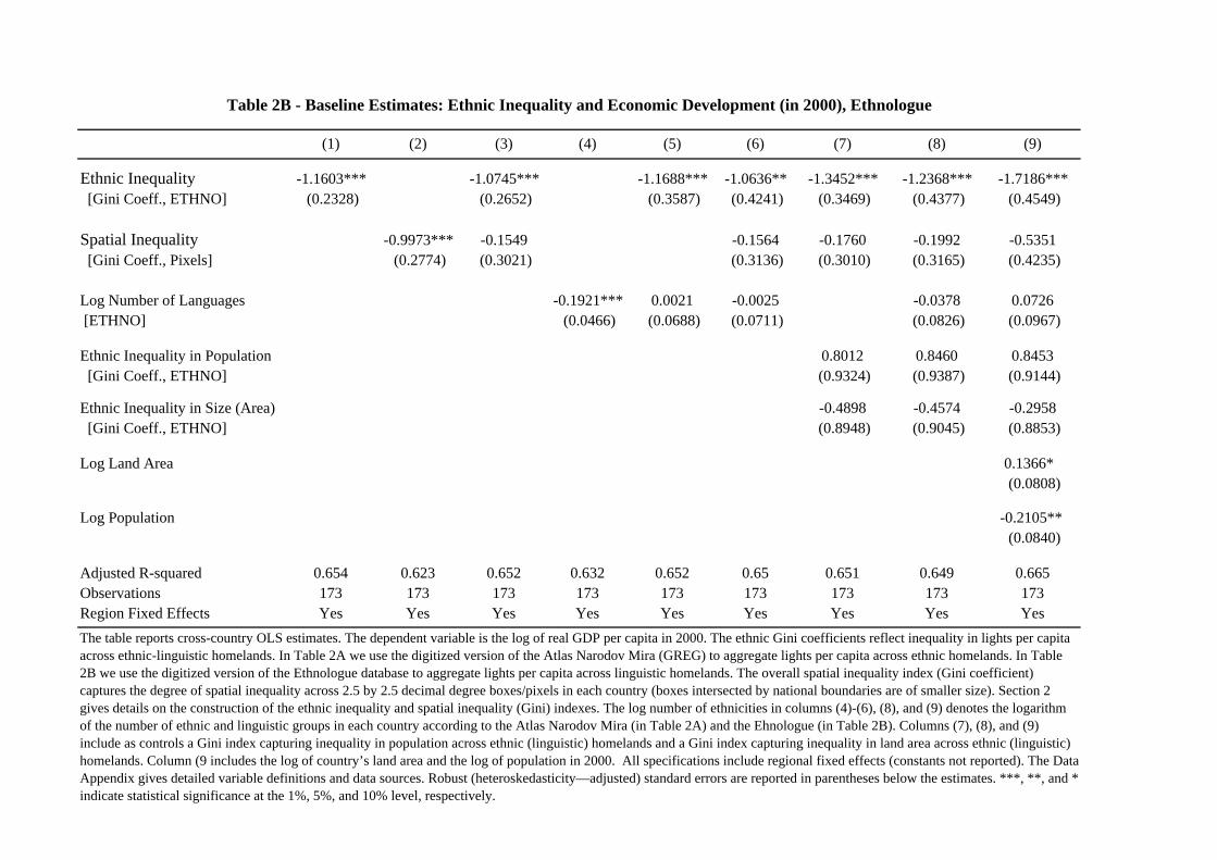
(1) (2) (3) (4) (5) (6) (7) (8) (9)

Ethnic Inequality -1.1603*** -1.0745*** -1.1688*** -1.0636** -1.3452*** -1.2368*** -1.7186*** [Gini Coeff., ETHNO] (0.2328) (0.2652) (0.3587) (0.4241) (0.3469) (0.4377) (0.4549)

Spatial Inequality -0.9973*** -0.1549 -0.1564 -0.1760 -0.1992 -0.5351 [Gini Coeff., Pixels] (0.2774) (0.3021) (0.3136) (0.3010) (0.3165) (0.4235)

Log Number of Languages -0.1921*** 0.0021 -0.0025 -0.0378 0.0726 [ETHNO] (0.0466) (0.0688) (0.0711) (0.0826) (0.0967)

Ethnic Inequality in Population 0.8012 0.8460 0.8453 [Gini Coeff., ETHNO] (0.9324) (0.9387) (0.9144)

Ethnic Inequality in Size (Area) -0.4898 -0.4574 -0.2958 [Gini Coeff., ETHNO] (0.8948) (0.9045) (0.8853)

Log Land Area 0.1366* (0.0808)

Log Population -0.2105** (0.0840)

Adjusted R-squared 0.654 0.623 0.652 0.632 0.652 0.65 0.651 0.649 0.665Observations 173 173 173 173 173 173 173 173 173Region Fixed Effects Yes Yes Yes Yes Yes Yes Yes Yes Yes

Table 2B - Baseline Estimates: Ethnic Inequality and Economic Development (in 2000), Ethnologue

The table reports cross-country OLS estimates. The dependent variable is the log of real GDP per capita in 2000. The ethnic Gini coefficients reflect inequality in lights per capita across ethnic-linguistic homelands. In Table 2A we use the digitized version of the Atlas Narodov Mira (GREG) to aggregate lights per capita across ethnic homelands. In Table 2B we use the digitized version of the Ethnologue database to aggregate lights per capita across linguistic homelands. The overall spatial inequality index (Gini coefficient) captures the degree of spatial inequality across 2.5 by 2.5 decimal degree boxes/pixels in each country (boxes intersected by national boundaries are of smaller size). Section 2 gives details on the construction of the ethnic inequality and spatial inequality (Gini) indexes. The log number of ethnicities in columns (4)-(6), (8), and (9) denotes the logarithm of the number of ethnic and linguistic groups in each country according to the Atlas Narodov Mira (in Table 2A) and the Ehnologue (in Table 2B). Columns (7), (8), and (9) include as controls a Gini index capturing inequality in population across ethnic (linguistic) homelands and a Gini index capturing inequality in land area across ethnic (linguistic) homelands. Column (9 includes the log of country’s land area and the log of population in 2000. All specifications include regional fixed effects (constants not reported). The Data Appendix gives detailed variable definitions and data sources. Robust (heteroskedasticity—adjusted) standard errors are reported in parentheses below the estimates. ***, **, and * indicate statistical significance at the 1%, 5%, and 10% level, respectively.

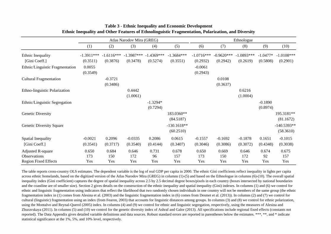
(1) (2) (3) (4) (5) (6) (7) (8) (9) (10)

Ethnic Inequality -1.3911*** -1.6116*** -1.3987*** -1.4369*** -1.3684*** -1.0716*** -0.9620*** -1.0893*** -1.0477* -1.0108*** [Gini Coeff.] (0.3511) (0.3876) (0.3478) (0.5274) (0.3551) (0.2932) (0.2942) (0.2619) (0.5808) (0.2901)

Ethnic/Linguistic Fragmentation 0.0055 -0.0061 (0.3549) (0.2943)

Cultural Fragmentation -0.3721 0.0108 (0.3486) (0.3637)

Ethno-linguistic Polarization 0.4442 0.6216 (1.0061) (1.0004)

Ethnic/Linguistic Segregation -1.3294* -0.1890 (0.7294) (0.8974)

Genetic Diversity 183.0360** 195.3181** (84.5187) (81.1672)

Genetic Diversity Square -130.1618** -140.5393** (60.2510) (58.3610)

Spatial Inequality -0.0021 0.2096 -0.0335 0.2086 0.0615 -0.1557 -0.1692 -0.1878 0.1651 -0.1015 [Gini Coeff.] (0.3541) (0.3717) (0.3540) (0.4144) (0.3407) (0.3046) (0.3086) (0.3072) (0.4348) (0.3038)

Adjusted R-square 0.650 0.684 0.646 0.731 0.678 0.650 0.669 0.646 0.674 0.675Observations 173 150 172 96 157 173 150 172 92 157Region Fixed Effects Yes Yes Yes Yes Yes Yes Yes Yes Yes Yes

Table 3 - Ethnic Inequality and Economic DevelopmentEthnic Inequality and Other Features of Ethnolinguistic Fragmentation, Polarization, and Diversity

Atlas Narodov Mira (GREG) Ethnologue

The table reports cross-country OLS estimates. The dependent variable is the log of real GDP per capita in 2000. The ethnic Gini coefficients reflect inequality in lights per capita across ethnic homelands, based on the digitized version of the Atlas Narodov Mira (GREG) in columns (1)-(5) and based on the Ethnologue in columns (6)-(10). The overall spatial inequality index (Gini coefficient) captures the degree of spatial inequality across 2.5 by 2.5 decimal degree boxes/pixels in each country (boxes intersected by national boundaries and the coastline are of smaller size). Section 2 gives details on the construction of the ethnic inequality and spatial inequality (Gini) indexes. In columns (1) and (6) we control for ethnic and linguistic fragmentation using indicators that reflect the likelihood that two randomly chosen individuals in one country will not be members of the same group (the ethnic fragmentation index in (1) comes from Alesina et al. (2003) and the linguistic fragmentation index in (6) comes from Desmet et al. (2013)). In columns (2) and (7) we control for cultural (linguistic) fragmentation using an index (from Fearon, 2003) that accounts for linguistic distances among groups. In columns (3) and (8) we control for ethnic polarization, using the Montalvo and Reynal-Querol (2005) index. In columns (4) and (9) we control for ethnic and linguistic segregation, respectively, using the measures of Alesina and Zhuravskaya (2011). In columns (5) and (10) we control for the genetic diversity index of Ashraf and Galor (2013). All specifications include regional fixed effects (constants not reported). The Data Appendix gives detailed variable definitions and data sources. Robust standard errors are reported in parentheses below the estimates. ***, **, and * indicate statistical significance at the 1%, 5%, and 10% level, respectively.

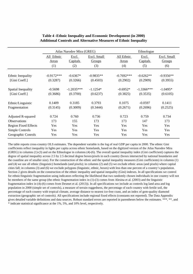
All Ethnic Areas

Excl. Capitals

Excl. Small Groups

All Ethnic Areas

Excl. Capitals

Excl. Small Groups

(1) (2) (3) (4) (5) (6)

Ethnic Inequality -0.9172*** -0.6367* -0.9835** -0.7692*** -0.6262** -0.9356** [Gini Coeff.] (0.3287) (0.3266) (0.4503) (0.2902) (0.2909) (0.3955)

Spatial Inequality -0.5698 -1.2035*** -1.1254* -0.6952* -1.3366*** -1.0495* [Gini Coeff.] (0.3686) (0.3700) (0.6237) (0.3825) (0.3535) (0.6105)

0.1409 0.3185 0.3793 0.1075 -0.0597 0.1411 (0.3145) (0.3009) (0.3444) (0.2671) (0.2696) (0.2525)

Adjusted R-squared 0.724 0.760 0.736 0.723 0.759 0.734Observations 173 155 173 173 147 173Region Fixed Effects Yes Yes Yes Yes Yes YesSimple Controls Yes Yes Yes Yes Yes YesGeographic Conrols Yes Yes Yes Yes Yes Yes

Ethnic/Linguistic Fragmentation

The table reports cross-country OLS estimates. The dependent variable is the log of real GDP per capita in 2000. The ethnic Gini coefficients reflect inequality in lights per capita across ethnic homelands, based on the digitized version of the Atlas Narodov Mira (GREG) in columns (1)-(3) and on the Ethnologue in columns (4)-(6). The overall spatial inequality index (Gini coefficient) captures the degree of spatial inequality across 2.5 by 2.5 decimal degree boxes/pixels in each country (boxes intersected by national boundaries and the coastline are of smaller size). For the construction of the ethnic and the spatial inequality measures (Gini coefficients) in columns (1) and (4) we use all ethnic (linguistic) homelands (and pixels); in columns (2) and (5) we exclude ethnic areas (and pixels) where capital cities fall; in columns (3) and (6) we exclude polygons (linguistic, ethnic, boxes) with less than one percent of a country’s population. Section 2 gives details on the construction of the ethnic inequality and spatial inequality (Gini) indexes. In all specifications we control for ethnic/linguistic fragmentation using indicators reflecting the likelihood that two randomly chosen individuals in one country will not be members of the same group (the ethnic fragmentation index in (1)-(3) comes from Alesina et al. (2003) and the linguistic fragmentation index in (4)-(6) comes from Desmet et al. (2013)). In all specifications we include as controls log land area and log population in 2000 (simple set of controls), a measure of terrain ruggedness, the percentage of each country with fertile soil, the percentage of each country with tropical climate, average distance to nearest ice-free coast, and an index of gem-quality diamond extraction (geographic set of controls). All specifications include regional fixed effects (constants not reported). The Data Appendix gives detailed variable definitions and data sources. Robust standard errors are reported in parentheses below the estimates. ***, **, and * indicate statistical significance at the 1%, 5%, and 10% level, respectively.

Ethnologue

Table 4 -Ethnic Inequality and Economic Development (in 2000)Additional Controls and Alternative Measures of Ethnic Inequality

Atlas Narodov Mira (GREG)

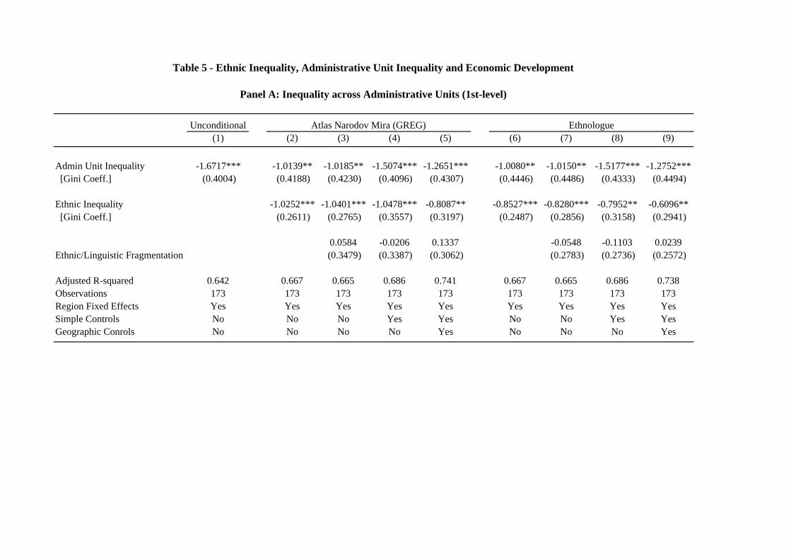
Unconditional(1) (2) (3) (4) (5) (6) (7) (8) (9)

Admin Unit Inequality -1.6717*** -1.0139** -1.0185** -1.5074*** -1.2651*** -1.0080** -1.0150** -1.5177*** -1.2752*** [Gini Coeff.] (0.4004) (0.4188) (0.4230) (0.4096) (0.4307) (0.4446) (0.4486) (0.4333) (0.4494)

Ethnic Inequality -1.0252*** -1.0401*** -1.0478*** -0.8087** -0.8527*** -0.8280*** -0.7952** -0.6096** [Gini Coeff.] (0.2611) (0.2765) (0.3557) (0.3197) (0.2487) (0.2856) (0.3158) (0.2941)

0.0584 -0.0206 0.1337 -0.0548 -0.1103 0.0239

(0.3479) (0.3387) (0.3062) (0.2783) (0.2736) (0.2572)

Adjusted R-squared 0.642 0.667 0.665 0.686 0.741 0.667 0.665 0.686 0.738Observations 173 173 173 173 173 173 173 173 173Region Fixed Effects Yes Yes Yes Yes Yes Yes Yes Yes YesSimple Controls No No No Yes Yes No No Yes YesGeographic Conrols No No No No Yes No No No Yes

Table 5 - Ethnic Inequality, Administrative Unit Inequality and Economic Development

Panel A: Inequality across Administrative Units (1st-level)

EthnologueAtlas Narodov Mira (GREG)

Ethnic/Linguistic Fragmentation

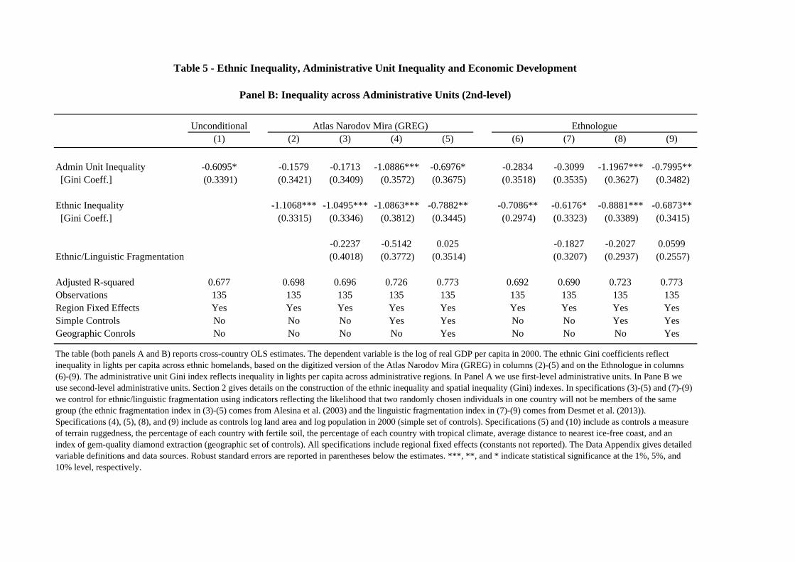
Unconditional(1) (2) (3) (4) (5) (6) (7) (8) (9)

Admin Unit Inequality -0.6095* -0.1579 -0.1713 -1.0886*** -0.6976* -0.2834 -0.3099 -1.1967*** -0.7995** [Gini Coeff.] (0.3391) (0.3421) (0.3409) (0.3572) (0.3675) (0.3518) (0.3535) (0.3627) (0.3482)

Ethnic Inequality -1.1068*** -1.0495*** -1.0863*** -0.7882** -0.7086** -0.6176* -0.8881*** -0.6873** [Gini Coeff.] (0.3315) (0.3346) (0.3812) (0.3445) (0.2974) (0.3323) (0.3389) (0.3415)

-0.2237 -0.5142 0.025 -0.1827 -0.2027 0.0599 (0.4018) (0.3772) (0.3514) (0.3207) (0.2937) (0.2557)

Adjusted R-squared 0.677 0.698 0.696 0.726 0.773 0.692 0.690 0.723 0.773Observations 135 135 135 135 135 135 135 135 135Region Fixed Effects Yes Yes Yes Yes Yes Yes Yes Yes YesSimple Controls No No No Yes Yes No No Yes YesGeographic Conrols No No No No Yes No No No Yes

The table (both panels A and B) reports cross-country OLS estimates. The dependent variable is the log of real GDP per capita in 2000. The ethnic Gini coefficients reflect inequality in lights per capita across ethnic homelands, based on the digitized version of the Atlas Narodov Mira (GREG) in columns (2)-(5) and on the Ethnologue in columns (6)-(9). The administrative unit Gini index reflects inequality in lights per capita across administrative regions. In Panel A we use first-level administrative units. In Pane B we use second-level administrative units. Section 2 gives details on the construction of the ethnic inequality and spatial inequality (Gini) indexes. In specifications (3)-(5) and (7)-(9) we control for ethnic/linguistic fragmentation using indicators reflecting the likelihood that two randomly chosen individuals in one country will not be members of the same group (the ethnic fragmentation index in (3)-(5) comes from Alesina et al. (2003) and the linguistic fragmentation index in (7)-(9) comes from Desmet et al. (2013)). Specifications (4), (5), (8), and (9) include as controls log land area and log population in 2000 (simple set of controls). Specifications (5) and (10) include as controls a measure of terrain ruggedness, the percentage of each country with fertile soil, the percentage of each country with tropical climate, average distance to nearest ice-free coast, and an index of gem-quality diamond extraction (geographic set of controls). All specifications include regional fixed effects (constants not reported). The Data Appendix gives detailed variable definitions and data sources. Robust standard errors are reported in parentheses below the estimates. ***, **, and * indicate statistical significance at the 1%, 5%, and 10% level, respectively.

Table 5 - Ethnic Inequality, Administrative Unit Inequality and Economic Development

Panel B: Inequality across Administrative Units (2nd-level)

Atlas Narodov Mira (GREG) Ethnologue

Ethnic/Linguistic Fragmentation

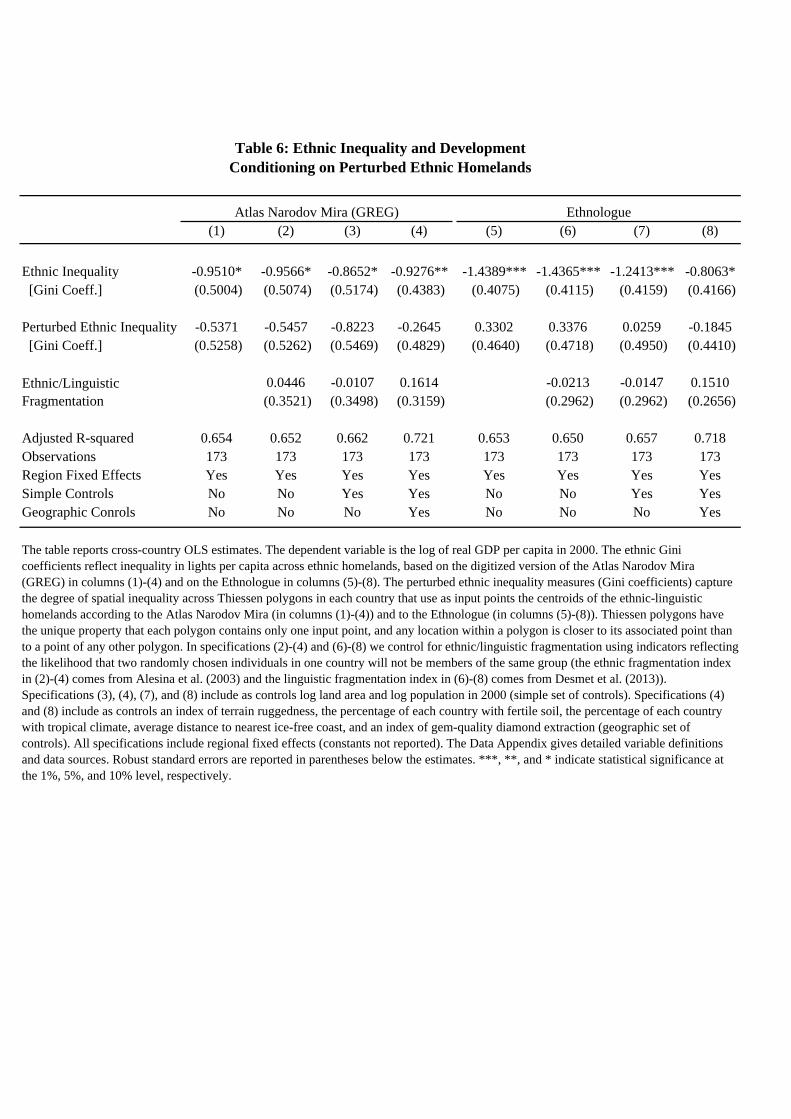
(1) (2) (3) (4) (5) (6) (7) (8)

Ethnic Inequality -0.9510* -0.9566* -0.8652* -0.9276** -1.4389*** -1.4365*** -1.2413*** -0.8063* [Gini Coeff.] (0.5004) (0.5074) (0.5174) (0.4383) (0.4075) (0.4115) (0.4159) (0.4166)

Perturbed Ethnic Inequality -0.5371 -0.5457 -0.8223 -0.2645 0.3302 0.3376 0.0259 -0.1845 [Gini Coeff.] (0.5258) (0.5262) (0.5469) (0.4829) (0.4640) (0.4718) (0.4950) (0.4410)

0.0446 -0.0107 0.1614 -0.0213 -0.0147 0.1510 (0.3521) (0.3498) (0.3159) (0.2962) (0.2962) (0.2656)

Adjusted R-squared 0.654 0.652 0.662 0.721 0.653 0.650 0.657 0.718Observations 173 173 173 173 173 173 173 173Region Fixed Effects Yes Yes Yes Yes Yes Yes Yes YesSimple Controls No No Yes Yes No No Yes YesGeographic Conrols No No No Yes No No No Yes

The table reports cross-country OLS estimates. The dependent variable is the log of real GDP per capita in 2000. The ethnic Gini coefficients reflect inequality in lights per capita across ethnic homelands, based on the digitized version of the Atlas Narodov Mira (GREG) in columns (1)-(4) and on the Ethnologue in columns (5)-(8). The perturbed ethnic inequality measures (Gini coefficients) capture the degree of spatial inequality across Thiessen polygons in each country that use as input points the centroids of the ethnic-linguistic homelands according to the Atlas Narodov Mira (in columns (1)-(4)) and to the Ethnologue (in columns (5)-(8)). Thiessen polygons have the unique property that each polygon contains only one input point, and any location within a polygon is closer to its associated point than to a point of any other polygon. In specifications (2)-(4) and (6)-(8) we control for ethnic/linguistic fragmentation using indicators reflecting the likelihood that two randomly chosen individuals in one country will not be members of the same group (the ethnic fragmentation index in (2)-(4) comes from Alesina et al. (2003) and the linguistic fragmentation index in (6)-(8) comes from Desmet et al. (2013)). Specifications (3), (4), (7), and (8) include as controls log land area and log population in 2000 (simple set of controls). Specifications (4) and (8) include as controls an index of terrain ruggedness, the percentage of each country with fertile soil, the percentage of each country with tropical climate, average distance to nearest ice-free coast, and an index of gem-quality diamond extraction (geographic set of controls). All specifications include regional fixed effects (constants not reported). The Data Appendix gives detailed variable definitions and data sources. Robust standard errors are reported in parentheses below the estimates. ***, **, and * indicate statistical significance at the 1%, 5%, and 10% level, respectively.

Table 6: Ethnic Inequality and Development Conditioning on Perturbed Ethnic Homelands

Atlas Narodov Mira (GREG) Ethnologue

Ethnic/Linguistic Fragmentation

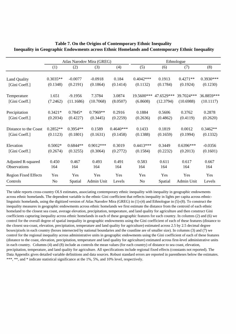
(1) (2) (3) (4) (5) (6) (7) (8)

Land Quality 0.3035** -0.0077 -0.0918 0.184 0.4042*** 0.1913 0.4271** 0.3930*** [Gini Coeff.] (0.1348) (0.2191) (0.1864) (0.1414) (0.1132) (0.1784) (0.1924) (0.1230)

Temperature 1.651 -9.1956 7.3784 3.0874 19.5600*** 47.6529*** 39.7024*** 36.8859*** [Gini Coeff.] (7.2462) (11.1686) (10.7068) (8.0507) (6.8608) (12.3794) (10.6988) (10.1117)

Precipitation 0.3421* 0.7845* 0.7969** 0.2916 0.1884 0.5606 0.3762 0.2878 [Gini Coeff.] (0.2034) (0.4227) (0.3445) (0.2259) (0.2636) (0.4862) (0.4119) (0.2620)

Distance to the Coast 0.2852** 0.3954** 0.1589 0.4640*** 0.1433 0.1819 0.0012 0.3462** [Gini Coeff.] (0.1123) (0.1801) (0.1631) (0.1458) (0.1388) (0.1659) (0.1994) (0.1332)

Elevation 0.5002* 0.6844** 0.9012*** 0.3019 0.4413*** 0.3449 0.6396*** -0.0356 [Gini Coeff.] (0.2674) (0.3255) (0.3064) (0.2772) (0.1584) (0.2232) (0.2013) (0.1601)

Adjusted R-squared 0.450 0.467 0.493 0.491 0.583 0.611 0.617 0.667Observations 164 164 164 164 164 164 164 164

Region Fixed Effects Yes Yes Yes Yes Yes Yes Yes Yes

Controls No Spatial Admin Unit Levels No Spatial Admin Unit Levels

The table reports cross-country OLS estimates, associating contemporary ethnic inequality with inequality in geographic endowments across ethnic homelands. The dependent variable is the ethnic Gini coefficient that reflects inequality in lights per capita across ethnic-linguistic homelands, using the digitized version of Atlas Narodov Mira (GREG) in (1)-(4) and Ethnologue in (5)-(8). To construct the inequality measures in geographic endowments across ethnic homelands we first estimate the distance from the centroid of each ethnic homeland to the closest sea coast, average elevation, precipitation, temperature, and land quality for agriculture and then construct Gini coefficients capturing inequality across ethnic homelands in each of these geographic features for each country. In columns (2) and (6) we control for the overall degree of spatial inequality in geographic endowments using the Gini coefficient of each of these features (distance to the closest sea-coast, elevation, precipitation, temperature and land quality for agriculture) estimated across 2.5 by 2.5 decimal degree boxes/pixels in each country (boxes intersected by national boundaries and the coastline are of smaller size). In columns (3) and (7) we control for the regional inequality across administrative units in geographic endowments using the Gini coefficient of each of these features (distance to the coast, elevation, precipitation, temperature and land quality for agriculture) estimated across first-level administrative units in each country. Columns (4) and (8) include as controls the mean values (for each country) of distance to sea coast, elevation, precipitation, temperature, and land quality for agriculture. All specifications include regional fixed effects (constants not reported). The Data Appendix gives detailed variable definitions and data sources. Robust standard errors are reported in parentheses below the estimates. ***, **, and * indicate statistical significance at the 1%, 5%, and 10% level, respectively.

Table 7. On the Origins of Contemporary Ethnic Inequality Inequality in Geographic Endowments across Ethnic Homelands and Contemporary Ethnic Inequality

Atlas Narodov Mira (GREG) Ethnologue

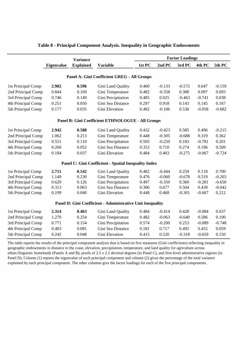
Eigenvalue Variable 1st PC 2nd PC 3rd PC 4th PC 5th PC

1st Principal Comp 2.982 0.596 Gini Land Quality 0.460 -0.133 -0.572 0.647 -0.1592nd Principal Comp 0.844 0.169 Gini Temperature 0.482 -0.358 0.388 0.097 0.6933rd Principal Comp 0.746 0.149 Gini Precipitation 0.485 0.025 -0.463 -0.741 0.0384th Principal Comp 0.251 0.050 Gini Sea Distance 0.297 0.918 0.143 0.145 0.1675th Principal Comp 0.177 0.035 Gini Elevation 0.482 -0.106 0.536 -0.058 -0.682

1st Principal Comp 2.942 0.588 Gini Land Quality 0.432 -0.423 0.585 0.496 -0.2152nd Principal Comp 1.062 0.213 Gini Temperature 0.448 -0.305 -0.688 0.319 0.3623rd Principal Comp 0.551 0.110 Gini Precipitation 0.505 -0.250 0.183 -0.781 0.2014th Principal Comp 0.260 0.052 Gini Sea Distance 0.353 0.710 0.274 0.196 0.5095th Principal Comp 0.184 0.037 Gini Elevation 0.484 0.403 -0.275 -0.067 -0.724

1st Principal Comp 2.711 0.542 Gini Land Quality 0.482 -0.444 0.259 0.118 0.7002nd Principal Comp 1.149 0.230 Gini Temperature 0.476 -0.060 -0.678 0.519 -0.2033rd Principal Comp 0.629 0.126 Gini Precipitation 0.497 -0.350 0.360 -0.281 -0.6504th Principal Comp 0.313 0.063 Gini Sea Distance 0.306 0.677 0.504 0.439 -0.0425th Principal Comp 0.199 0.040 Gini Elevation 0.448 0.468 -0.301 -0.667 0.212

1st Principal Comp 2.314 0.463 Gini Land Quality 0.484 -0.414 0.428 -0.084 0.6372nd Principal Comp 1.270 0.254 Gini Temperature 0.482 -0.063 -0.640 0.586 0.1003rd Principal Comp 0.771 0.154 Gini Precipitation 0.574 -0.200 0.253 -0.089 -0.7484th Principal Comp 0.403 0.081 Gini Sea Distance 0.181 0.717 0.492 0.455 0.0595th Principal Comp 0.242 0.048 Gini Elevation 0.415 0.520 -0.318 -0.659 0.150

The table reports the results of the principal component analysis that is based on five measures (Gini coefficients) reflecting inequality in geographic endowments in distance to the coast, elevation, precipitation, temperature, and land quality for agriculture across ethnic/linguistic homelands (Panels A and B), pixels of 2.5 x 2.5 decimal degrees (in Panel C), and first-level administrative regions (in Panel D). Column (1) reports the eigenvalue of each principal component and column (2) gives the percentage of the total variance explained by each principal component. The other columns give the factor loadings for each of the five principal components.

Panel C: Gini Coefficient - Spatial Inequality Index

Panel D: Gini Coefficient - Administrative Unit Inequality

Factor Loadings

Table 8 - Principal Component Analysis. Inequality in Geographic Endowments

Variance Explained

Panel A: Gini Coefficient GREG - All Groups

Panel B: Gini Coefficient ETHNOLOGUE - All Groups

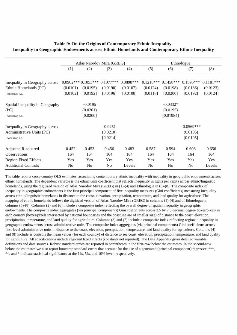
(1) (2) (3) (4) (5) (6) (7) (8)

0.0902*** 0.1053*** 0.1077*** 0.0898*** 0.1210*** 0.1458*** 0.1595*** 0.1181***(0.0101) (0.0195) (0.0190) (0.0107) (0.0124) (0.0198) (0.0186) (0.0123)

bootstrap s.e. [0.0102] [0.0192] [0.0196] [0.0108] [0.0118] [0.0200] [0.0192] [0.0124]

-0.0195 -0.0332*(0.0201) (0.0195)

bootstrap s.e. [0.0200] [0.01984]

-0.0251 -0.0569***(0.0210) (0.0185)

bootstrap s.e. [0.0214] [0.0195]

Adjusted R-squared 0.452 0.453 0.456 0.483 0.587 0.594 0.608 0.656Observations 164 164 164 164 164 164 164 164Region Fixed Effects Yes Yes Yes Yes Yes Yes Yes YesAdditional Controls No No No Levels No No No Levels

The table reports cross-country OLS estimates, associating contemporary ethnic inequality with inequality in geographic endowments across ethnic homelands. The dependent variable is the ethnic Gini coefficient that reflects inequality in lights per capita across ethnic/linguistic homelands, using the digitized version of Atlas Narodov Mira (GREG) in (1)-(4) and Ethnologue in (5)-(8). The composite index of inequality in geographic endowments is the first principal component of five inequality measures (Gini coefficients) measuring inequality across ethnic/linguistic homelands in distance to the coast, elevation, precipitation, temperature, and land quality for agriculture. The mapping of ethnic homelands follows the digitized version of Atlas Narodov Mira (GREG) in columns (1)-(4) and of Ethnologue in columns (5)-(8). Columns (2) and (6) include a composite index reflecting the overall degree of spatial inequality in geographic endowments. The composite index aggregates (via principal components) Gini coefficients across 2.5 by 2.5 decimal degree boxes/pixels in each country (boxes/pixels intersected by national boundaries and the coastline are of smaller size) of distance to the coast, elevation, precipitation, temperature, and land quality for agriculture. Columns (3) and (7) include a composite index reflecting regional inequality in geographic endowments across administrative units. The composite index aggregates (via principal components) Gini coefficients across first-level administrative units in distance to the coast, elevation, precipitation, temperature, and land quality for agriculture. Columns (4) and (8) include as controls the mean values (for each country) of distance to sea coast, elevation, precipitation, temperature, and land quality for agriculture. All specifications include regional fixed effects (constants not reported). The Data Appendix gives detailed variable definitions and data sources. Robust standard errors are reported in parentheses in the first-row below the estimates. In the second-row below the estimates we also report bootstrap standard errors that account for the use of a generated (principal component) regressor. ***, **, and * indicate statistical significance at the 1%, 5%, and 10% level, respectively.

Inequality in Geography across Administrative Units (PC)

Table 9: On the Origins of Contemporary Ethnic Inequality Inequality in Geographic Endowments across Ethnic Homelands and Contemporary Ethnic Inequality

Atlas Narodov Mira (GREG) Ethnologue

Inequality in Geography across Ethnic Homelands (PC)

Spatial Inequality in Geography (PC)

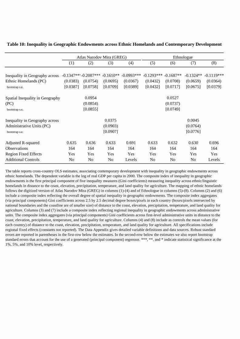
(1) (2) (3) (4) (5) (6) (7) (8)

-0.1347***-0.2087*** -0.1610** -0.0993*** -0.1293*** -0.1687** -0.1324** -0.1119***(0.0383) (0.0754) (0.0695) (0.0367) (0.0432) (0.0708) (0.0659) (0.0364)

bootstrap s.e. [0.0387] [0.0758] [0.0709] [0.0389] [0.0432] [0.0717] [0.0675] [0.0379]

0.0954 0.0527(0.0854) (0.0737)

bootstrap s.e. [0.0855] [0.0749]

0.0375 0.0045(0.0903) (0.0764)

bootstrap s.e. [0.0907] [0.0776]

Adjusted R-squared 0.635 0.636 0.633 0.691 0.633 0.632 0.630 0.696Observations 164 164 164 164 164 164 164 164Region Fixed Effects Yes Yes Yes Yes Yes Yes Yes YesAdditional Controls No No No Levels No No No Levels

The table reports cross-country OLS estimates, associating contemporary development with inequality in geographic endowments across ethnic homelands. The dependent variable is the log of real GDP per capita in 2000. The composite index of inequality in geographic endowments is the first principal component of five inequality measures (Gini coefficients) measuring inequality across ethnic/linguistic homelands in distance to the coast, elevation, precipitation, temperature, and land quality for agriculture. The mapping of ethnic homelands follows the digitized version of Atlas Narodov Mira (GREG) in columns (1)-(4) and of Ethnologue in columns (5)-(8). Columns (2) and (6) include a composite index reflecting the overall degree of spatial inequality in geographic endowments. The composite index aggregates (via principal components) Gini coefficients across 2.5 by 2.5 decimal degree boxes/pixels in each country (boxes/pixels intersected by national boundaries and the coastline are of smaller size) of distance to the coast, elevation, precipitation, temperature, and land quality for agriculture. Columns (3) and (7) include a composite index reflecting regional inequality in geographic endowments across administrative units. The composite index aggregates (via principal components) Gini coefficients across first-level administrative units in distance to the coast, elevation, precipitation, temperature, and land quality for agriculture. Columns (4) and (8) include as controls the mean values (for each country) of distance to the coast, elevation, precipitation, temperature, and land quality for agriculture. All specifications include regional fixed effects (constants not reported). The Data Appendix gives detailed variable definitions and data sources. Robust standard errors are reported in parentheses in the first-row below the estimates. In the second-row below the estimates we also report bootstrap standard errors that account for the use of a generated (principal component) regressor. ***, **, and * indicate statistical significance at the 1%, 5%, and 10% level, respectively.

Ethnologue

Inequality in Geography across Ethnic Homelands (PC)

Spatial Inequality in Geography (PC)

Inequality in Geography across Administrative Units (PC)

Table 10: Inequality in Geographic Endowments across Ethnic Homelands and Contemporary Development

Atlas Narodov Mira (GREG)

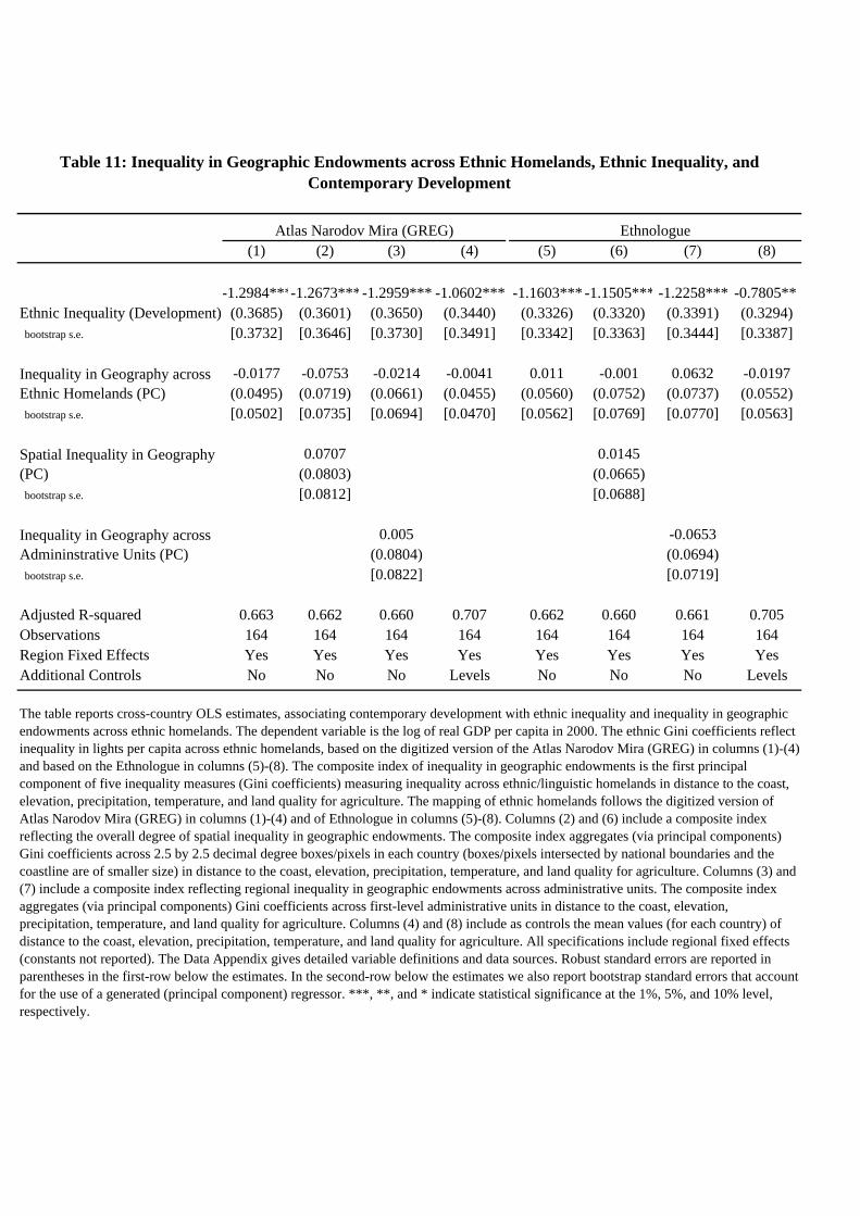
(1) (2) (3) (4) (5) (6) (7) (8)

-1.2984***-1.2673***-1.2959*** -1.0602*** -1.1603*** -1.1505*** -1.2258*** -0.7805** (0.3685) (0.3601) (0.3650) (0.3440) (0.3326) (0.3320) (0.3391) (0.3294)

bootstrap s.e. [0.3732] [0.3646] [0.3730] [0.3491] [0.3342] [0.3363] [0.3444] [0.3387]

-0.0177 -0.0753 -0.0214 -0.0041 0.011 -0.001 0.0632 -0.0197(0.0495) (0.0719) (0.0661) (0.0455) (0.0560) (0.0752) (0.0737) (0.0552)

bootstrap s.e. [0.0502] [0.0735] [0.0694] [0.0470] [0.0562] [0.0769] [0.0770] [0.0563]

0.0707 0.0145(0.0803) (0.0665)

bootstrap s.e. [0.0812] [0.0688]

0.005 -0.0653(0.0804) (0.0694)

bootstrap s.e. [0.0822] [0.0719]

Adjusted R-squared 0.663 0.662 0.660 0.707 0.662 0.660 0.661 0.705Observations 164 164 164 164 164 164 164 164Region Fixed Effects Yes Yes Yes Yes Yes Yes Yes YesAdditional Controls No No No Levels No No No Levels

The table reports cross-country OLS estimates, associating contemporary development with ethnic inequality and inequality in geographic endowments across ethnic homelands. The dependent variable is the log of real GDP per capita in 2000. The ethnic Gini coefficients reflect inequality in lights per capita across ethnic homelands, based on the digitized version of the Atlas Narodov Mira (GREG) in columns (1)-(4) and based on the Ethnologue in columns (5)-(8). The composite index of inequality in geographic endowments is the first principal component of five inequality measures (Gini coefficients) measuring inequality across ethnic/linguistic homelands in distance to the coast, elevation, precipitation, temperature, and land quality for agriculture. The mapping of ethnic homelands follows the digitized version of Atlas Narodov Mira (GREG) in columns (1)-(4) and of Ethnologue in columns (5)-(8). Columns (2) and (6) include a composite index reflecting the overall degree of spatial inequality in geographic endowments. The composite index aggregates (via principal components) Gini coefficients across 2.5 by 2.5 decimal degree boxes/pixels in each country (boxes/pixels intersected by national boundaries and the coastline are of smaller size) in distance to the coast, elevation, precipitation, temperature, and land quality for agriculture. Columns (3) and (7) include a composite index reflecting regional inequality in geographic endowments across administrative units. The composite index aggregates (via principal components) Gini coefficients across first-level administrative units in distance to the coast, elevation, precipitation, temperature, and land quality for agriculture. Columns (4) and (8) include as controls the mean values (for each country) of distance to the coast, elevation, precipitation, temperature, and land quality for agriculture. All specifications include regional fixed effects (constants not reported). The Data Appendix gives detailed variable definitions and data sources. Robust standard errors are reported in parentheses in the first-row below the estimates. In the second-row below the estimates we also report bootstrap standard errors that account for the use of a generated (principal component) regressor. ***, **, and * indicate statistical significance at the 1%, 5%, and 10% level, respectively.

Spatial Inequality in Geography (PC)

Inequality in Geography across Admininstrative Units (PC)

Inequality in Geography across Ethnic Homelands (PC)

Table 11: Inequality in Geographic Endowments across Ethnic Homelands, Ethnic Inequality, and Contemporary Development

Atlas Narodov Mira (GREG) Ethnologue

Ethnic Inequality (Development)