Embed Size (px)
Citation preview
CNMG Master ETHZ – BAUG – FS2014
26. August 2014 S e i t e | 1 Christoph Hager
CONSTITUTIVE MODELLING IN GEOMECHANICS © chager – Version 2014 - 1.0 Prof. A.M.Puzrin, ETHZ
INTRODUTION C1
BOU NDAR Y V ALU E P ROBL EM 6
ODO ME TER T EST 7
TRIAX IAL T EST
SOIL S 7, 8
Soils are Multiphase, Granular, non-homogeneous, anisotropic Soils behave:
Non-linear (initial loading, unloading, reloading)
Irreversible (residual strains in closed stress cycle)
Has a memory (remember highest stresses before unloading)
Stress-path dependency (same stress at different strains)
Rete dependent (diff. stress-strain curves at diff strain rates)
Time dependent (creep, aging, relaxation)
EQ. OF CONTINUUM MECH C5
EQU AT ION S 5 4
MOTI ON
Moments:
Equilibrium:
COM PATIB I LI TY
Geometric:
( )
CONS TI TU TIV E R E LATI O NS HIP
Form of ( )
Is a model and are different for each material. (Equilibrium and compatibility relations are always the same)
CR are simplifications and approximations → Model
INITIA L A ND B OU NDARY C ONDI TI ONS
Initial values of stress and/or displacements have to be specified. Normally equal to zero.
Static boundary conditions define displacements on sections
Kinematic BC define traction → stresses
Mixed BC combine both → i.e. shear traction Relationship between displ. And traction also possible
2D S IMPL IF IC AT IO N S 5 6
PLA NE S TRAI N
Principal strain in one direction is zero
For retaining walls, strip found., trench excavation, tunnel
PLA NE S TR ESS
Principal stress in one direction is zero
Fir Cavity expansion of borehole
AXISYMM E TRIC
EX AMPL E 5 7
An analytical example is provided in the book on page57
FINITE ELEMETS C6 → see also Mech II, UTB I
APPL IC AT IO N 6 4
1) Discretization → FE between nodes, unknown displ. 2) Shape functions → define displ. within elements 3) Compability equations → define strains in element 4) Constitutive relationships → define stresses in elements 5) Equilibrium equations for each element → stiffness matrix 6) Equilibrium equations for each node sum all nodal forces 7) Static/kinematic boundary conditions reduce unknowns 8) Solution → displacements, stresses and strains
Examples p65, 72, Implementation Appendix B p295
FINITE DIFFERENCES C7 Not of interest (p84)
EQ. OF CONT. THERMODYNAMICS C8 Not of interest (p101)
CONSTITUTIVE MODELING INTRODUCTION C9
OV ER V IEW 110
Soils are multiphase, granular, non-homogeneous, anisotropic Behavior can be: non-linear, stress path dependent, stress level dependent, irreversible, material memory, dilatancy, hardening, rete dependent, time dependent
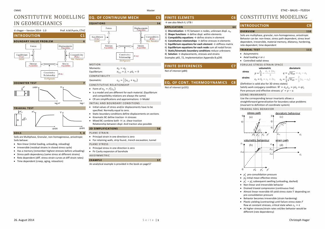
TRIAX IAL T EST 111
Axisymmetric
Axial loading or
Controlled radial stress
FOR ULAS S TRESS -S TRAI N S PAC E
volumetric deviatoric
stress
√
strains
√
( )
(Definition is valid also for 3D stress states)
Satisfy work conjugacy condition:
Pore pressure and effective stresses:
US I NG I NVARIA NTS
Use the corresponding tensor invariants allows a straightforward generalization for boundary value problems (invariant to definition of coordinate system)
TR IAXIA L S OI L B E HAVI OR
pre-consolidation pressure
initial mean effective stress
subsequent swelling (unloading, dashed)
Non-linear and irreversible behavior
Drained triaxial compression (continuous line)
Almost linear reversible till yield stress state depending on pre-consolidation pressure
Behavior becomes irreversible (strain hardening)
Plastic yielding (contracting) until failure stress state flow at constant stresses, critical state when
At higher stresses/strain rates vol/dev behavior would be different (rate dependency)
CNMG Master ETHZ – BAUG – FS2014
26. August 2014 S e i t e | 2 Christoph Hager
ELEMENTARY TENSOR ANALYSIS C2 → Use indices instead of a matrix, calculations are implicit the same. Attention if term is a scalar, vector or tensor!
IN DIC IAL N OTAT IO N 1 2- 15
Basic:
{
}
[
]
Free: Represents Position (axis) → number of equations Dummy: Ongoing number, subcalculations from known matrix-operations, placeholder → summation in index notation
Free index appears once in each term
Dummy index appears twice and denotes summation
Dummy index can be replaced without changing result
Index cannot appear three times in same term ( )
Partial differentiation is denoted by a comma
(
)
(
)
(
)
Kroneker Delta:
[
]
{
→
Properties:
( )
→ Multiplication with replace dummy with free index
SC ALAR S, V ECT OR S, T EN SOR S 1 5- 21
Scalar no index or only dummy index
Vector 1. order object, only one free index
Tensor 2. order object, two free indices
Transformation (of the system) → p16./p.18
(inverse)
[
]
Rotation of the system:
Rotation of a vector/matrix:
TE NS OR INVARIA NTS 1 9
( ⁄ )
( ⁄ )
CHARAC T ERISTI C EQ UA T ION 2 0
→ Plane where vector is perpend. to this plane (principal axis)
| |
( )
Characteristic Equation: are principal quantities Coefficients = Invariants: (Function of Tensor invariants)
( )
|
| |
| |
|
[ ]
( ) ( )
|
|
[ ]
Char Eq: Stress: Strain:
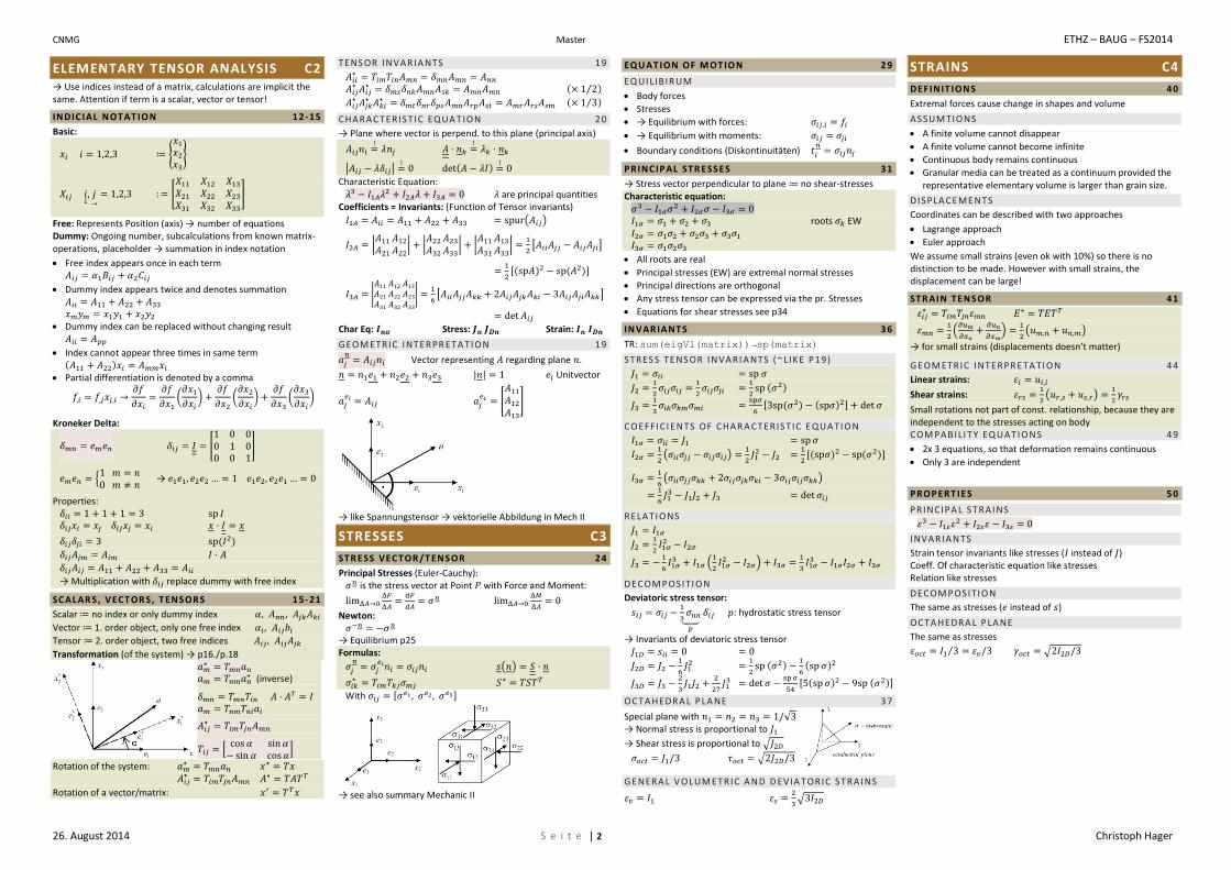
GE OM ETRIC I NT ERPR E TA TI ON 1 9
Vector representing regarding plane .
Unitvector
[
]
→ like Spannungstensor → vektorielle Abbildung in Mech II
STRESSES C3
STR E SS VEC TOR /T EN SOR 2 4
Principal Stresses (Euler-Cauchy): is the stress vector at Point with Force and Moment:
Newton: → Equilibrium p25 Formulas:
( )
With
→ see also summary Mechanic II
EQU AT ION OF M OT IO N 2 9
EQ UI LIB IRUM
Body forces
Stresses
→ Equilibrium with forces:
→ Equilibrium with moments:
Boundary conditions (Diskontinuitäten)
PRINC IP AL STR E SSE S 3 1
→ Stress vector perpendicular to plane no shear-stresses Characteristic equation: roots EW
All roots are real
Principal stresses (EW) are extremal normal stresses
Principal directions are orthogonal
Any stress tensor can be expressed via the pr. Stresses
Equations for shear stresses see p34
IN V AR IA NT S 3 6
TR: sum(eigVl(matrix))→sp(matrix)
STRES S TE NS OR INVARI A NTS ( ~ LIK E P19)
( )
( ) ( )
COEFF ICI E NTS OF CHAR A CT ERIS TIC E QUA TI ON
( )
( ) ( )
( )
RELA TI ONS
(
)
DEC OM P OSITI ON
Deviatoric stress tensor:
⏟
: hydrostatic stress tensor
→ Invariants of deviatoric stress tensor
( )
( )
( ) ( )
OC TA HEDRA L P LA NE 3 7
Special plane with √ → Normal stress is proportional to
→ Shear stress is proportional to √
√
GE NERA L V OLUM E TRIC A ND D EVIA T ORIC S TRAI NS
√
STRAINS C4
DEF IN IT ION S 4 0
Extremal forces cause change in shapes and volume
ASSUM TIONS
A finite volume cannot disappear
A finite volume cannot become infinite
Continuous body remains continuous
Granular media can be treated as a continuum provided the representative elementary volume is larger than grain size.
D ISPLA CE ME NTS
Coordinates can be described with two approaches
Lagrange approach
Euler approach
We assume small strains (even ok with 10%) so there is no distinction to be made. However with small strains, the displacement can be large!
STR AIN TE N SOR 4 1
(
)
( )
→ for small strains (displacements doesn’t matter)
GE OM ETRIC I NT ERPR E TA TI ON 4 4
Linear strains:
Shear strains:
( )
Small rotations not part of const. relationship, because they are independent to the stresses acting on body COM PABILI T Y EQ UA TI ON S 4 9
2x 3 equations, so that deformation remains continuous
Only 3 are independent
PROP ERT IE S 5 0
PRINCIPA L S TRAI NS
INVARIA NTS
Strain tensor invariants like stresses ( instead of ) Coeff. Of characteristic equation like stresses Relation like stresses
DEC OM P OSITI ON
The same as stresses ( instead of )
OC TA HEDRA L P LA NE
The same as stresses
⁄ √
CNMG Master ETHZ – BAUG – FS2014
26. August 2014 S e i t e | 3 Christoph Hager
Reversible soil behavior, small strains:
LINEAR ISOTROPIC ELASTICITY C10
OV ER V IEW 118
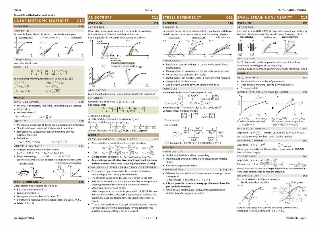
PROPER TI ES
Reversible, linear elastic, isotropic, completely uncoupled
APP LICA TION
Works for elastic part
FORM ULA S
{
} [
] {
}
By decoupling following relations can be found (p123):
√ √
√
√
MOD ELS
E LASTI C B EHA VIOR 119
Material is completely reversible, unloading equals loading
Hooke’s low
Stiffness matrix
I SOTROPY 120
Mechanical properties all the same in all geometric directions
Simplify stiffness matrix to 2 independent quantities
Expression via stress/strain tensor invariants only for isotropic materials
Definition: ( )
L I NEARI T Y+IS OTR OPY 121
Isotropic relation becomes liner when: and
Physical meaning: (define old Lame’s elastic constants using known behavior)
ELA ST IC CO N ST ANT S 125
Linear elastic model can be described by:
Bulk and shear moduli
Lame constants
Young modulus and Poisson’s ration
Constrained modulus and rest lateral pressure coeff.
→ Table 10.1 p126
ANISOTROPY C11
OV ER V IEW 132
PROPER TI ES
Reversible, anisotropic, coupled → invariants not working! Material behave different in different direction Coupling leads to stress path dependency of stiffness
APP LICA TION
Main impact in tunneling, in our problems not that important
FORM ULA S
General cross-anisotropy → (11.8)-(11.10) For triaxial test:
{
} [
] {
}
: coupling modulus : bulk modulus, isotropic consolidation : shear modulus pure shear
Are not invariants! ( ) → (11.19-11.21) p139
MOD ELS
CROSS A NIS OT R OP Y , L I NEAR E LAST IC 135
Differentiation of vertical and horizontal directions
z:
(
) (
)
x, (y):
(
) (
)
5 independent constants:
An anisotropic constitutive law cannot expressed via stress and strain tensor invariants (coupling, dependent of axis)
COUP LI NG A ND S TRESS D EP E ND E NCY OF S TIFF N ESS
Cross-anisotropic linear elastic for triax test → develop relationships p138-139 → provided model
The stiffness depends on the direction of the stress path
In isotropic consolidation and pure shear the model produce coupling between deviatoric and volumetric behavior
Model can cause serious errors: while the general cross-anisotropic model (11.8)-(11.10) can always simulate the stress path dependency of stiffness and coupling (11.18) in a triaxial test, the inverse statement is wrong
Triaxial compression and isotropic consolidation test are not sufficient for derive the parameters for the general cross-anisotropic model. (Only 3 out of 5 known)
STRESS DEPENDENCY C12
OV ER V IEW 146
PROPER TI ES
Reversible, secant shear and bulk stiffness are higher with larger initial stresses (same pre-consolidation), hardening behavior
APP LICA TION
Results can vary very widely in contrary to isotropic linear elastic model.
Main problem in examples are not accurate pressure level
Porous elastic is an important model
Useful model, but not the reality → not sure what happens
Overpredicts displacements
Good for pre-yielding deviatoric behavior in triax
FORM ULA S
Hypoelasticity (Violates Thermodynamic law)
{
} [
( )
( )
] {
}
(
)
Hyperelasticity: (Thermodyn ok, see also book, p151ff) Constant-shear-modulus model:
{
} [
] {
}
Linear model:
{
}
[
(
)
]
{
}
, coupled, only for uncoupled →
MOD ELS
HY P OE LAS TIC Y 147
Useful tool, flexible and less demanding
Inelastic, not always integrable and can produce residual strains
Violates energy conservation!
HY PER E LAS TIC Y (148) 151
Different Models which don’t violates law of energy conserv. -Constant -Linear model → only for
It is not possible to have no energy problem and have the poisson ratio constant
Plaxis porous elastic model with constant poisson ratio violates low of energy conservation!
SMALL STRAIN NONLINEARITY C13
OV ER V IEW 156
PROPER TI ES
For small strains (0.01-0.1%), (irreversible), non-linear, softening behavior. Underestimate G at small strains → overest. displ.
APP LICA TION
For Problems with wide range of small strains, Initial Shear Modulus is much higher at the beginning. Multiple surface kinematic hardening plasticity-model works too
MOD ELS
REQ UIRE ME NTS 157
Simple, minimum number of parameters
Clear physical meaning, easy to derive from tests
Provide good fit
NORMA LIZ ED PR E-YI E LDI NG B E HAV IOR 157
Conditions to be satisfied: : approx. with straight line 1) 2) ⁄
HY PERB OLIC FU NCTI ON 159
Approach:
Param. i.e. (Cond2) ,
Not really working: Not both cond. Can be satisfied
RAMBERG - OSG OOD 160
Approach:
More ugly, but satisfy both conditions, implement in ABAQUS Path still too straight
LOGARIT HMIC 160
Approach: ( )
Parameters: ( ) ( )
(
)
( )
Good! Function has correct shape, high level of non-linearity at very small strains, both conditions satisfied.
IRREV ERSIB IL I T Y 161
Elastic model with 3 different behaviors:
Masing rule: Reloading curve is backbone curve factor 2, unloading is like reloading one →
CNMG Master ETHZ – BAUG – FS2014
26. August 2014 S e i t e | 4 Christoph Hager
Irreversible soil behavior:
FAILURE C14
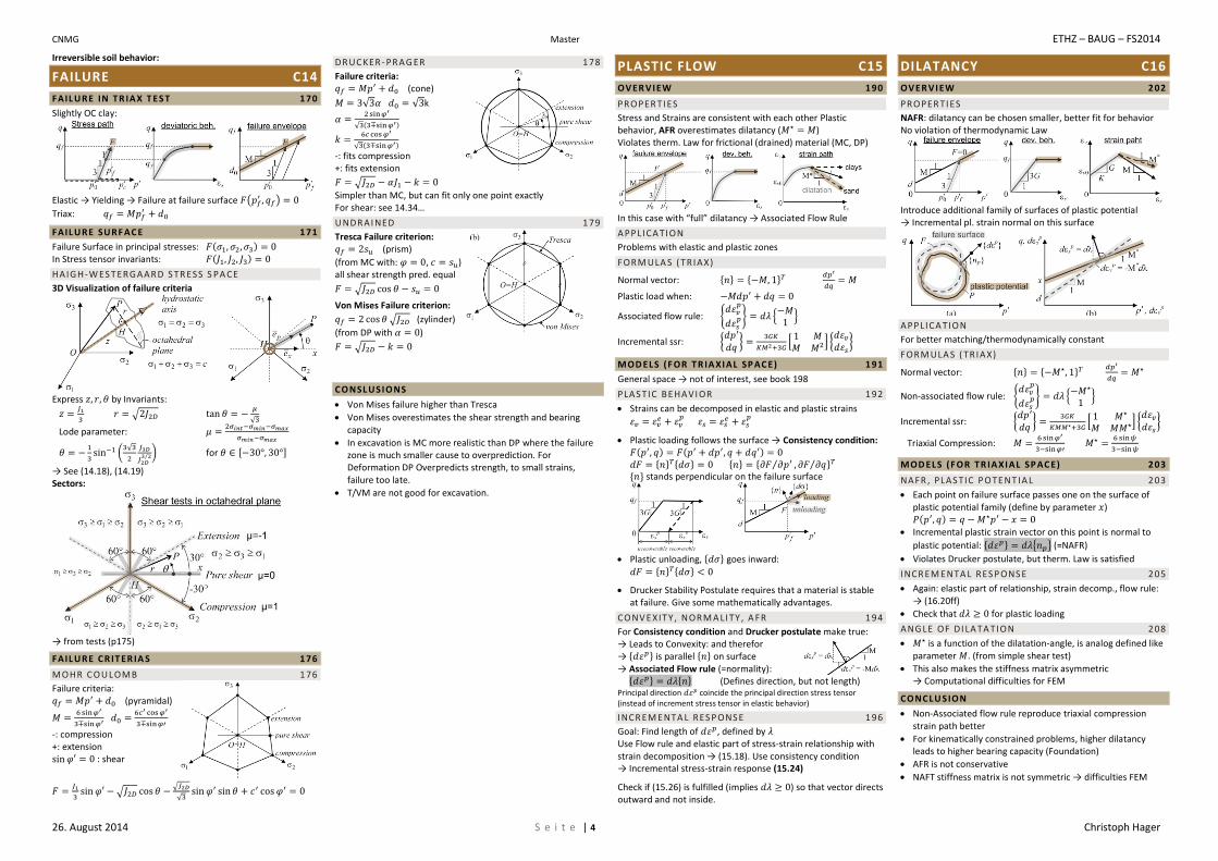
FAIL URE IN TR IA X T E S T 170
Slightly OC clay:
Elastic → Yielding → Failure at failure surface (
)
Triax:
FAIL URE SURF AC E 171
Failure Surface in principal stresses: ( ) In Stress tensor invariants: ( )
HAIGH-W ES T ERGAARD S TR ESS S PA CE
3D Visualization of failure criteria
Express by Invariants:
√
√
Lode parameter:
(
√
⁄ ) for
→ See (14.18), (14.19) Sectors:
→ from tests (p175)
FAIL URE CR IT ER IA S 176
MOHR C OU LOMB 176
Failure criteria: (pyramidal)
-: compression +: extension : shear
√
√
√
DRUC KER - PRAG ER 178
Failure criteria: (cone)
√ √ k
√ ( )
√ ( )
-: fits compression +: fits extension
√
Simpler than MC, but can fit only one point exactly For shear: see 14.34…
U NDRAI NED 179
Tresca Failure criterion: (prism)
(from MC with: , ) all shear strength pred. equal
√
Von Mises Failure criterion:
√ (zylinder)
(from DP with )
√
CO NSL USIO NS
Von Mises failure higher than Tresca
Von Mises overestimates the shear strength and bearing capacity
In excavation is MC more realistic than DP where the failure zone is much smaller cause to overprediction. For Deformation DP Overpredicts strength, to small strains, failure too late.
T/VM are not good for excavation.
PLASTIC FLOW C15
OV ER V IEW 190
PROPER TI ES
Stress and Strains are consistent with each other Plastic behavior, AFR overestimates dilatancy ( ) Violates therm. Law for frictional (drained) material (MC, DP)
In this case with “full” dilatancy → Associated Flow Rule
APP LICA TION
Problems with elastic and plastic zones
FORM ULA S ( TR IAX)
Normal vector: { } { }
Plastic load when:
Associated flow rule: {
} {
}
Incremental ssr: {
}
[ ] {
}
MOD ELS (F OR TR IA XIAL SP AC E) 191
General space → not of interest, see book 198
PLAS TIC BE HAVI OR 192
Strains can be decomposed in elastic and plastic strains
Plastic loading follows the surface → Consistency condition: ( ) ( ) { } { } { } { ⁄ ⁄ } { } stands perpendicular on the failure surface
Plastic unloading, { } goes inward:
{ } { }
Drucker Stability Postulate requires that a material is stable at failure. Give some mathematically advantages.
CONV E XIT Y , NORM A LI TY , A FR 194
For Consistency condition and Drucker postulate make true: → Leads to Convexity: and therefor → { } is parallel { } on surface → Associated Flow rule (=normality): { } { } (Defines direction, but not length) Principal direction coincide the principal direction stress tensor (instead of increment stress tensor in elastic behavior)
INCR EM E NTA L RES P ONS E 196
Goal: Find length of , defined by Use Flow rule and elastic part of stress-strain relationship with strain decomposition → (15.18). Use consistency condition → Incremental stress-strain response (15.24)
Check if (15.26) is fulfilled (implies ) so that vector directs outward and not inside.
DILATANCY C16
OV ER V IEW 202
PROPER TI ES
NAFR: dilatancy can be chosen smaller, better fit for behavior No violation of thermodynamic Law
Introduce additional family of surfaces of plastic potential → Incremental pl. strain normal on this surface
APP LICA TION
For better matching/thermodynamically constant
FORM ULA S ( TR IAX)
Normal vector: { } { }
Non-associated flow rule: {
} {
}
Incremental ssr: {
}
[
] {
}
Triaxial Compression:
MOD ELS (F OR TR IA XIAL SP AC E) 203
NAFR , PLAS TIC P OTE NT IA L 203
Each point on failure surface passes one on the surface of plastic potential family (define by parameter ) ( )
Incremental plastic strain vector on this point is normal to
plastic potential: { } { } (=NAFR)
Violates Drucker postulate, but therm. Law is satisfied
INCR EM E NTA L RES P ONS E 205
Again: elastic part of relationship, strain decomp., flow rule: → (16.20ff)
Check that for plastic loading
ANG LE OF DI LA TA TION 208
is a function of the dilatation-angle, is analog defined like parameter . (from simple shear test)
This also makes the stiffness matrix asymmetric → Computational difficulties for FEM
CO NCLU SIO N
Non-Associated flow rule reproduce triaxial compression strain path better
For kinematically constrained problems, higher dilatancy leads to higher bearing capacity (Foundation)
AFR is not conservative
NAFT stiffness matrix is not symmetric → difficulties FEM
CNMG Master ETHZ – BAUG – FS2014
26. August 2014 S e i t e | 5 Christoph Hager
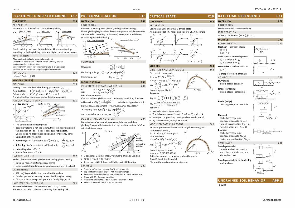
PLASTIC YIELDING+STR HARDNG C17
OV ER V IEW 214
PROPER TI ES
Models plastic flow before failure, shear yielding
Plastic yielding can occur before failure. After an unloading-reloading circle the yielding starts at a higher point → hardening
APP LICA TION Triax: deviatoric behavior good, volumetric not Foundation: Behave now softer → better, VM only for pure compression/failure is the same. Excavation: VM no diff here (not near failure → eff. stresses), DP much better for failure and yielding (softer behavior)
FORM ULA S 223
→ See (17.41), (17.42)
MOD ELS (T RIAX ) 215
YIE LDI NG 215
Yielding is described with hardening parameters
Yield surface: ( ) (
) (
)
Failure surface: ( ) The yield surface can evolve during loading-processes
HARDE NI NG /S OF TE NI NG 215
The Strains can be decomposed
Because yielding is not the failure, there is no restriction on the direction of { } → this is called plastic loading. One can also find loading condition and consistency cond.
Unloading behave elastic.
Hardening: Surface expands { } { } ,
Softening: Surface contract { } { } ,
Unloading when
Plastic flow when
HARDE NI NG RU LE 217
→ describes evolution of yield surface during plastic loading
Isotropic hardening: Surface is centered
(other possibilities: kinematic, combined, perfect → failure)
DEF I NITI ONS
AFR:
is parallel to the normal to the surface
Drucker postulate can only be satisfies during hardening
Dilatancy: introduce plastic potential family ( )
INCR EM E NTA L RES P ONS E 221
Incremental stress-strain response → (17.37), (17.41) Particular case with cohesive hardening (linear) → p223
PRE-CONSOLIDATION C18
OV ER V IEW 230
PROPER TI ES
Volumetric yielding with plastic yielding and hardening Plastic yielding begins when the current pre-consolidation stress is exceeded in reloading (Volumetric). New pre-consolidation stress is higher → hardening.
FORM ULA S
Flow rule: {
} {
}
Hardening rule: (
)
(
)
Incremental ssr:
MOD ELS (T RIAX ) 231
VOLUM ETRIC S TRAIN HA R DE NI NG 231
VCL:
URL:
Procedure as always: -Decomposition, yield surface, consistency condition, flow rule
-el behavior: ( ) ( )
(similar to hypoelastic vol,
but not constant anymore → thermodynamic consistency)
-Hardening rule: (
)
(
)
-incremental response:
DOUBLE HARD E NI NG → C A P 234
Combination of volumetric (pre-consolidation) and shear yielding → cap model cause to the cap on shear surface in 3D in principal stress space
3 Zones for yielding: shear, volumetric or mixed yielding
Yield in zone I → shrinks
In corner → NAFR, leads in FEM to math. Difficulties
EXAM P LE 237
Smooth surface, but complex, NAFR, non-symmetric
Cap yield surface as an ellipse - AFR with same shape
Between a transition yield surface, also elliptical - NAFR same shape
Shear with DP - Same as transition
Hardening rule controls size of cap and transition surface
Relates pre-consol. to vol. pl. strain. as usual
CRITICAL STATE C19
OV ER V IEW 242
PROPER TI ES
Constant volume shearing → critical state All in one model: PC, hardening, Failure, CS, AFR, simple
MOD ELS 243
ORIGI NAL CAM C LA Y M O D E L 243
Zero elastic shear strain
, ( ) ( )
AFR: {
} {
}
Hardening rule like left Response:
( (
) (
))
⁄ ( ⁄ )
( ⁄ )
Behavior:
Neglects elastic shear strains
Triaxial compression → wet ( before ) or dry, ok
Isotropic compression, develops shear strain, not ok
consolidation, to high → not ok
MODIF I ED CAM CLA Y M O DE L 246
→ Solves problem with overpredicting shear strength in compression and . Elastic: , like original Elliptical shape
AFR: {
} {
(
)
}
Hardening rule as always response → (19.41), (19.42) Better because of rectangular end on the p-axis Beautiful and simple model. Fits also thermodynamics consistency.
RATE+TIME DEPENDENCY C21
OV ER V IEW 270
PROPER TI ES
Model time and rate dependency
INTEG TRA TION
→ See p274 formula (21.10), (21.11)
MOD ELS 271
FU NDAM E NTA L 271
Hookean – perfectly elastic
Yield stress – perfectly plastic when
when
Newtonian – perfectly viscous
→ creep / rate dep. Strength
COM P OSIT 273
St. Venant elastic-plastic behavior
Linear Hardening elastic-plastic (hardening)
Kelvin (Voigt) decaying creep, recoverable
Maxwell partially irrecoverable, constant creep rate ( ) total stress relaxation ( ) rate dep shear str. ( )
Bingham partially irrecoverable, constant creep rate ( )
partial stress relaxation ( )
TW O- LAY ER 280
Two-layer-model rate dependency of shear str. with plastic and viscous rate dependent part.
Two-layer-model + lin hardening analog above
UNDRAINED SOIL BEHAVIOR APP A → p289

CNMG Master ETHZ – BAUG – FS2014
26. August 2014 S e i t e | 6 Christoph Hager
EXERCISES/EXAMPLE EXAM
EXERCISES FEM example: Ex1 Implementing geometry in ABAQUS Ex2 Isotropic elastic Ex3 Derive from triaxial test over Stress dependency [porous elastic] Ex4 Negative Poisson ratio Derive from triaxial test (Small Strain) Nonlinear Elasticity [deform pl.] Ex5 Ramberg-Osgood Normalization Derive Mohr Coulomb Ex6 Derive from triaxial test Drucker Prager Ex7 Derive from triaxial test Gebastel mit plane strain Yielding/Hardening Ex8 VM, Tresca, simulate cohesionless hardening Critical State Ex9 Derive from triaxial test Rate Dependency Ex10
HOMEWORKS Index Notation, Invariants H1 Elastic models (el, stress dep, nonlin) H2 Parameter derivation, plots Plastic models (MC, DP, VM, Tresca) H3 Parameter derivation, plots Analytical bearing capacity Smother Übergang El-pl? Matching wichtig? Yielding in wall-problem? Modified Cam Clay H4 Parameter derivation, plots
ELASTIC CONSTANTS
MODELING
MAK IN G MOD EL
-el behavior and its definition (matrix-term) -decomposition for
-yield/failure surface -consistency condition
-flow rule {
} { }
-other conditions like hardening… -insert FR, other cond. in CC, solve to -insert into flow rule → into matrix-term -leading to incremental response
EXAM P LES:
El-pl AFR p196 El-pl NAFR p203 El-pl hardening P221 El-vol strain hardening p231 Org Cam clay p243 MCC p249 Cr-anisotr-pl AFR Example exam
VARIA
FAQ
THE ORY Formel (12.3) und (11.1) sollen eigentlich falsch sein (Buch s134, „are
intrinsically wrong“ zB) Was ist damit gemeint?
Models aren’t coupled → just a model
Gilt Isotropic linear elasticity in triaxial space (10.1) auch für expansion?
Es wird ja immer der compression stress path angeschaut…
Ja, hebt sich mit 3/2G anstatt 3G auf.
Wie sind und für pure shear beim Drucker-Prager-Modell definiert
(Formel 14.34)? Kann hier unter dem Bruchstrich in Formeln
(14.37) gesetzt werden?
Ja, sollte funktionieren
Parameterfitting bei MC-DP (1 Folie nach why matching, der
Übungsbesprechung): wieso gibt es hier bei plane strain 2 verschiedene
für AFR und NAFR. entspricht ja eigentlich (nicht ) so wie
wir das verstanden haben?
Das Ganze ist relativ kompliziert: Bei NAFR ist eigentlich kein effektives
Matching möglich, da failure load nicht eindeutig bestimmt ist.
Bei Plane Strain passt DP-cone nicht überall auf MC-Oberfläche. Stück
dazwischen verhält sich wie „hardening“ mit teilplastischen Elementen,
Modell ist aber vollständig elastisch. Belastung muss nun DP-cone so
treffen (bestimmt durch ) damit dann schlussendlich bei Erreichen der
MC Oberfläche die richtige Richtung des Normalenvektors (Thermodyn
+ Fliessrichtung) resultiert. Diese ist aber eben auch von der Belastung
und dem Initialzustand abhängig, ist also nicht eindeutig definiert.
EX AMPL E- EX AM
Task 1: Hier erhalten wir als Lösung einen dreidimensionalen
Dehnungszustand, also drei verschiedene Hauptdehnungen.
Ist es dennoch möglich Volumetrische oder Deviatorische
Dehnungen zu berechnen. Respektive gilt
√ allgemein?
Ja gilt allgemein, sollte noch im Buch ergänzt werden
Task 4: Wodurch entstehen diese Wellenlinien bei NAFR. Ist
das wegen dem Modellverhalten, oder hat dies einen
numerischen Hintergrund?
Nicht nur, grösstenteils wegen nicht eindeutig definierter
failure load → Verhalten sehr sensitiv/“instabil“ welche
Bereiche sich plastifizieren wegen NAFR
EX AM
Ist es in Ordnung die Matrixschreibweise anstatt die
Indexschreibweise zu verwenden (solange es Formal korrekt
ist?
zB:
( ) anstatt
Jep
EXK URS TU N NELB AU
Softening-Modelle sind gefährlich: Durch diese entstehen Scherbänder mit unbekannter Breite → Scherdehnungen unbekannt, somit auch Scherparameter. In FEM bilden sich diese meist in einem Element aus → FEM-Grösse muss mit Scherbandbreiten kalibriert werden!
EXAM SUMMER 2014
MIT N EHM EN A N PRÜFU N G
Buch CNMG
Folien
Übungen, Übungsbesprechung
ZF Analysis
ZF Linalg
ZF Mechanik I+II
ZF Baustatik
ZF Bodenmechanik
ZF Geotechnik
EX AM SUMM ER 2014
Couldn’t remember all the questions, but hope you get an idea: 1. Tensor analysis [~21P]
Given Tensor: [
]
a) Calculating Eigenvalues, Eigenvectors b) Which parameter for fitting vonMises c) Tresca and vonMises fitting for cutting wall 5m high d) How to control FEM? (Analytical h=… given) 2. Develop const. model (incremental response) [~30P]
Linear elasticity, vol. hardening (similar to book, but given function with ( ) instead ( )), NAFR DP. → develop incremental response (like example exam)
3. Mechanical Model [~23P]
(for p greater than py) a) p=¢, calculate in way like ( ) b) Parameter derivation, you got 2 tests (different p) with
given graph and table ( for ). Solution from a) provided in
c) what would change if creep rate at the end is constant, change model (graphically) and draw graph (qualitative)
d) After which time will the creep rate be at 10% 4. MCC [~26P] a) 2 tests from same sample → derive pc and M given were 2 graphs (p-q and -?), test A didn’t reach Y, at a given point softening starts but wasn’t shown in graph, test B reaches Y, but not F b) M=0.8, is plausible? c) is clay normally consolidated? (OCR<2) d) …? 2 and 3 were similar to example exam. Actual Exam was much broader, parameter fitting is important. TEBM knowledge helps. Some questions gave a lot of points (like 1a…) and were very easy to calculate. But overall exam was not that easy and the grades were given tough ;]