Embed Size (px)
Citation preview
ETM 607 – Discrete Event Simulation Fundamentals
• Define Discrete Event Simulation.
• Define concepts (entities, attributes, event list, etc…)
• Define “world-view”, or how discrete event simulation operates
• Example hand simulation
ETM 607 – Discrete Event Simulation Fundamentals
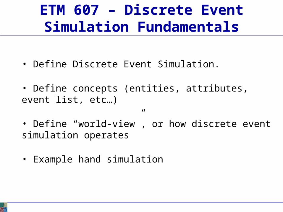
• System – a collection of entities that act and interact toward the accomplishment of some logical end.
• State – the state of a system is the collection of variables necessary to describe the status of the system at any given time.
• Discrete – a discrete system is one in which the state variables change only at discrete or countable points in time.
• Continuous– a continuous system is one in which the state variables change continuously over time.
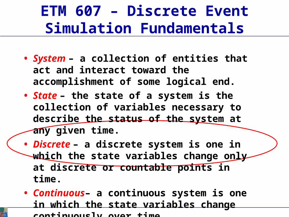
• Static – a static simulation model is a representation of a system at a particular point in time.
• Dynamic – a dynamic simulation is a representation of a system as it evolves over time.
• Deterministic – a deterministic simulation model is one that contains no random variables. All variables are known with certainty, or in other words, no probability is associated with them.
• Stochastic– a stochastic simulation model contains random variables (variables containing probability distributions).
ETM 607 – Discrete Event Simulation Fundamentals
Pieces of a Simulation Model
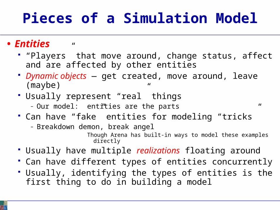
• Entities “Players” that move around, change status, affect and are
affected by other entities Dynamic objects — get created, move around, leave
(maybe) Usually represent “real” things
– Our model: entities are the parts Can have “fake” entities for modeling “tricks”
– Breakdown demon, break angelThough Arena has built-in ways to model these examples
directly
Usually have multiple realizations floating around Can have different types of entities concurrently Usually, identifying the types of entities is the first thing to
do in building a model
Pieces of a Simulation Model (cont’d.)
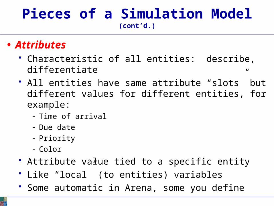
• Attributes Characteristic of all entities: describe, differentiate All entities have same attribute “slots” but different values
for different entities, for example:– Time of arrival– Due date– Priority– Color
Attribute value tied to a specific entity Like “local” (to entities) variables Some automatic in Arena, some you define
Pieces of a Simulation Model (cont’d.)
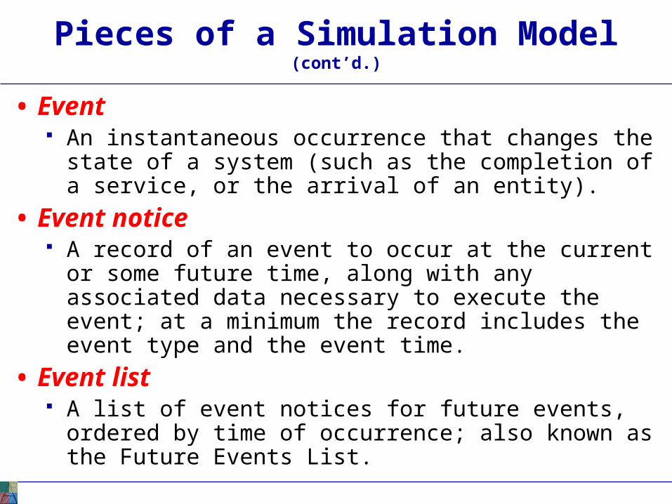
• Event An instantaneous occurrence that changes the state of a
system (such as the completion of a service, or the arrival of an entity).
• Event notice A record of an event to occur at the current or some future
time, along with any associated data necessary to execute the event; at a minimum the record includes the event type and the event time.
• Event list A list of event notices for future events, ordered by time of
occurrence; also known as the Future Events List.
Pieces of a Simulation Model (cont’d.)
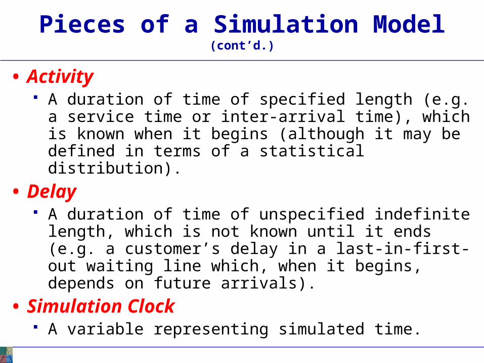
• Activity A duration of time of specified length (e.g. a service time or
inter-arrival time), which is known when it begins (although it may be defined in terms of a statistical distribution).
• Delay A duration of time of unspecified indefinite length, which is
not known until it ends (e.g. a customer’s delay in a last-in-first-out waiting line which, when it begins, depends on future arrivals).
• Simulation Clock A variable representing simulated time.
Pieces of a Simulation Model (cont’d.)
• Resources What entities compete for
– People– Equipment– Space
Entity seizes a resource, uses it, releases it Think of a resource being assigned to an entity, rather than
an entity “belonging to” a resource “A” resource can have several units of capacity
– Seats at a table in a restaurant– Identical ticketing agents at an airline counter
Number of units of resource can be changed during the simulation
Pieces of a Simulation Model (cont’d.)
• Queues Place for entities to wait when they can’t move on (maybe
since the resource they want to seize is not available) Have names, often tied to a corresponding resource Can have a finite capacity to model limited space — have
to model what to do if an entity shows up to a queue that’s already full
Usually watch the length of a queue, waiting time in it
Pieces of a Simulation Model (cont’d.)
• Statistical accumulators Variables that “watch” what’s happening Depend on output performance measures desired “Passive” in model — don’t participate, just watch Many are automatic in Arena, but some you may have to
set up and maintain during the simulation At end of simulation, used to compute final output
performance measures
Pieces of a Simulation Model (cont’d.)
• Statistical accumulators for the simple processing system Number of parts produced so far Total of the waiting times spent in queue so far No. of parts that have gone through the queue Max time in queue we’ve seen so far Total of times spent in system Max time in system we’ve seen so far Area so far under queue-length curve Q(t) Max of Q(t) so far Area so far under server-busy curve B(t)
Simulation Dynamics:The Event-Scheduling “World View”
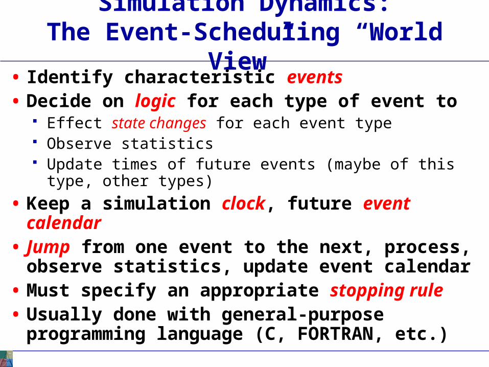
• Identify characteristic events• Decide on logic for each type of event to
Effect state changes for each event type Observe statistics Update times of future events (maybe of this type, other
types)
• Keep a simulation clock, future event calendar• Jump from one event to the next, process,
observe statistics, update event calendar• Must specify an appropriate stopping rule• Usually done with general-purpose programming
language (C, FORTRAN, etc.)
The System:A Simple Processing System
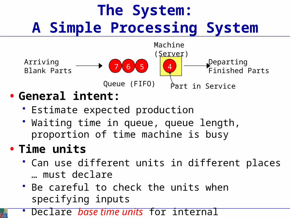
ArrivingBlank Parts
DepartingFinished Parts
Machine(Server)
Queue (FIFO) Part in Service
4567
• General intent: Estimate expected production Waiting time in queue, queue length, proportion of time
machine is busy
• Time units Can use different units in different places … must declare Be careful to check the units when specifying inputs Declare base time units for internal calculations, outputs Be reasonable (interpretation, roundoff error)
Model Specifics
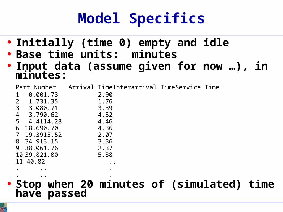
• Initially (time 0) empty and idle• Base time units: minutes• Input data (assume given for now …), in minutes:
Part Number Arrival Time Interarrival Time Service Time1 0.00 1.73 2.902 1.73 1.35 1.763 3.08 0.71 3.394 3.79 0.62 4.525 4.41 14.28 4.466 18.69 0.70 4.367 19.39 15.52 2.078 34.91 3.15 3.369 38.06 1.76 2.37
10 39.82 1.00 5.3811 40.82 . .
. . . .
. . . .
• Stop when 20 minutes of (simulated) time have passed
Goals of the Study:Output Performance Measures
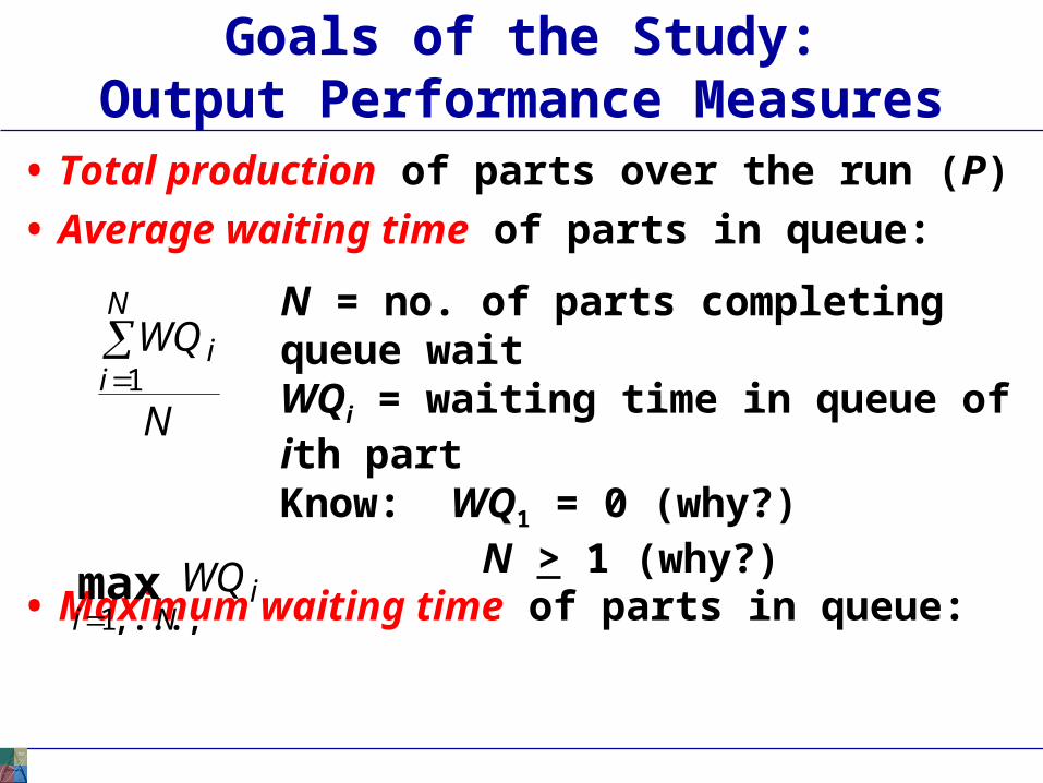
• Total production of parts over the run (P)
• Average waiting time of parts in queue:
• Maximum waiting time of parts in queue:
N = no. of parts completing queue waitWQi = waiting time in queue of ith partKnow: WQ1 = 0 (why?)
N > 1 (why?)N
WQN
ii
1
iNi
WQmax,...,1
Goals of the Study:Output Performance Measures (cont’d.)
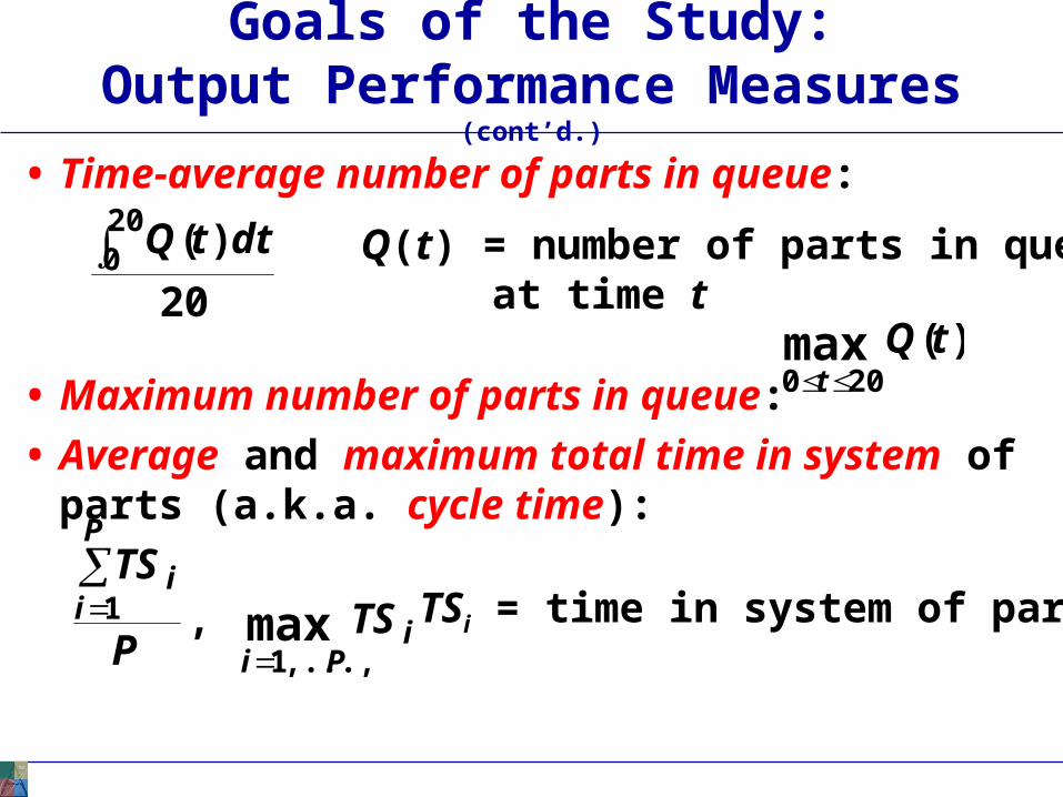
• Time-average number of parts in queue:
• Maximum number of parts in queue:
• Average and maximum total time in system of parts (a.k.a. cycle time):
Q(t) = number of parts in queue at time t20
)(200 dttQ
)(max200
tQt
iPi
P
ii
TSP
TS
max,...,1
1 ,
TSi = time in system of part i
Goals of the Study:Output Performance Measures (cont’d.)
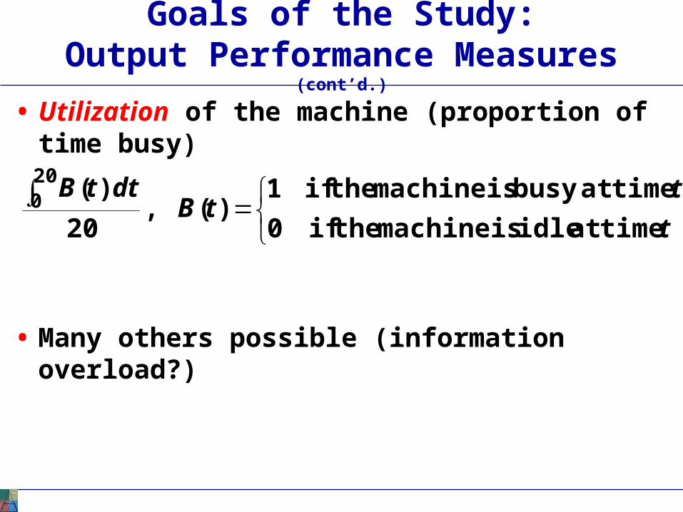
• Utilization of the machine (proportion of time busy)
• Many others possible (information overload?)
t
ttB
dttB
timeat idle is machine the if0
timeat busy is machine the if1)(,
20
)(200
Events for theSimple Processing System
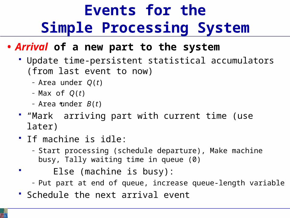
• Arrival of a new part to the system Update time-persistent statistical accumulators (from last
event to now)– Area under Q(t)– Max of Q(t)– Area under B(t)
“Mark” arriving part with current time (use later) If machine is idle:
– Start processing (schedule departure), Make machine busy, Tally waiting time in queue (0)
Else (machine is busy):– Put part at end of queue, increase queue-length variable
Schedule the next arrival event
Events for theSimple Processing System (cont’d.)
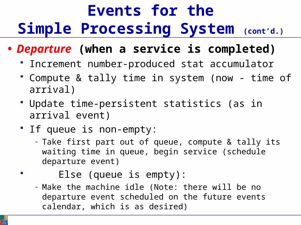
• Departure (when a service is completed) Increment number-produced stat accumulator Compute & tally time in system (now - time of arrival) Update time-persistent statistics (as in arrival event) If queue is non-empty:
– Take first part out of queue, compute & tally its waiting time in queue, begin service (schedule departure event)
Else (queue is empty):– Make the machine idle (Note: there will be no departure event
scheduled on the future events calendar, which is as desired)
Events for theSimple Processing System (cont’d.)
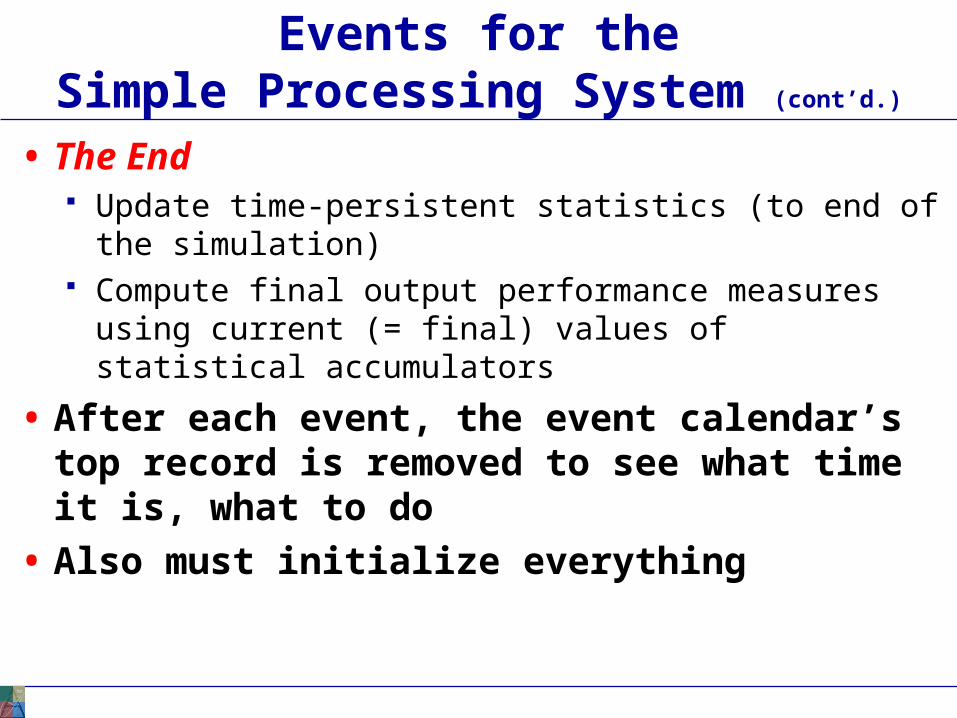
• The End Update time-persistent statistics (to end of the simulation) Compute final output performance measures using current
(= final) values of statistical accumulators
• After each event, the event calendar’s top record is removed to see what time it is, what to do
• Also must initialize everything
Some Additional Specifics for theSimple Processing System
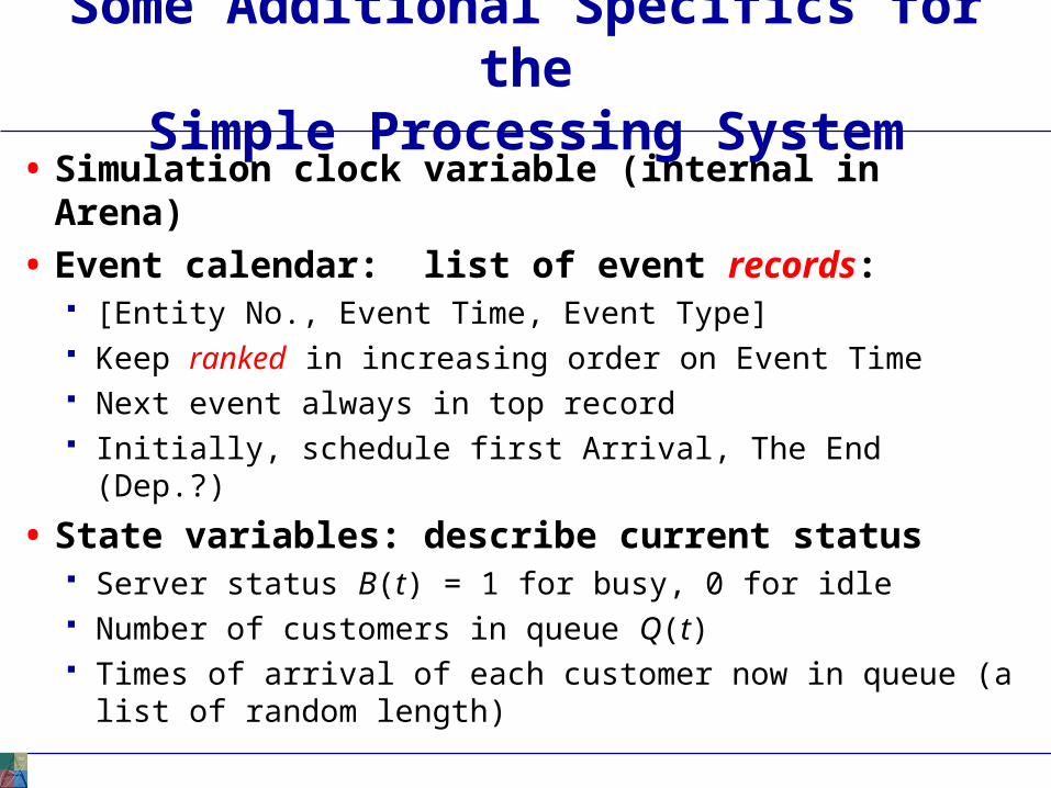
• Simulation clock variable (internal in Arena)
• Event calendar: list of event records: [Entity No., Event Time, Event Type] Keep ranked in increasing order on Event Time Next event always in top record Initially, schedule first Arrival, The End (Dep.?)
• State variables: describe current status Server status B(t) = 1 for busy, 0 for idle Number of customers in queue Q(t) Times of arrival of each customer now in queue (a list of
random length)
Simulation by Hand
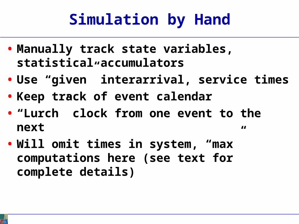
• Manually track state variables, statistical accumulators
• Use “given” interarrival, service times
• Keep track of event calendar
• “Lurch” clock from one event to the next
• Will omit times in system, “max” computations here (see text for complete details)
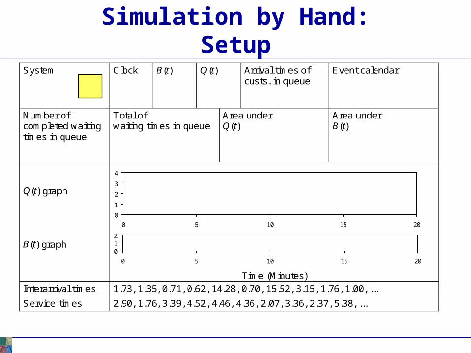
System
Clock
B(t)
Q(t)
Arrival times of custs. in queue
Event calendar
Number of completed waiting times in queue
Total of waiting times in queue
Area under Q(t)
Area under B(t)
Q(t) graph B(t) graph
Time (Minutes) Interarrival times 1.73, 1.35, 0.71, 0.62, 14.28, 0.70, 15.52, 3.15, 1.76, 1.00, ...
Service times 2.90, 1.76, 3.39, 4.52, 4.46, 4.36, 2.07, 3.36, 2.37, 5.38, ...
Simulation by Hand:Setup
0
1
2
3
4
0 5 10 15 20
012
0 5 10 15 20
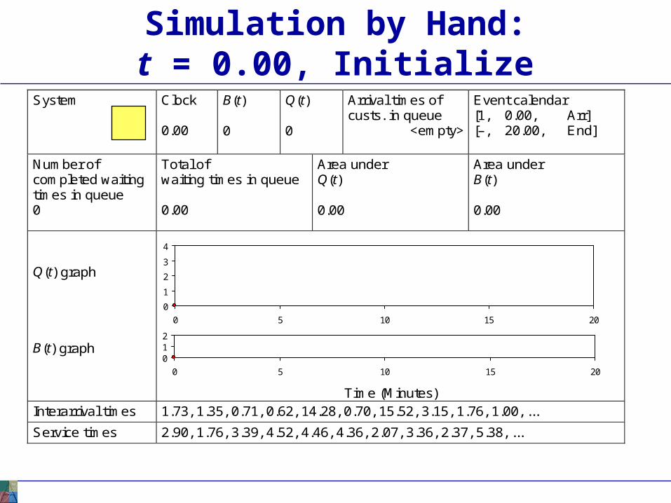
System
Clock 0.00
B(t) 0
Q(t) 0
Arrival times of custs. in queue
<empty>
Event calendar [1, 0.00, Arr] [–, 20.00, End]
Number of completed waiting times in queue 0
Total of waiting times in queue 0.00
Area under Q(t) 0.00
Area under B(t) 0.00
Q(t) graph B(t) graph
Time (Minutes) Interarrival times 1.73, 1.35, 0.71, 0.62, 14.28, 0.70, 15.52, 3.15, 1.76, 1.00, ...
Service times 2.90, 1.76, 3.39, 4.52, 4.46, 4.36, 2.07, 3.36, 2.37, 5.38, ...
Simulation by Hand:t = 0.00, Initialize
0
1
2
3
4
0 5 10 15 20
012
0 5 10 15 20
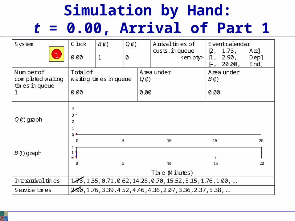
System
Clock 0.00
B(t) 1
Q(t) 0
Arrival times of custs. in queue
<empty>
Event calendar [2, 1.73, Arr] [1, 2.90, Dep] [–, 20.00, End]
Number of completed waiting times in queue 1
Total of waiting times in queue 0.00
Area under Q(t) 0.00
Area under B(t) 0.00
Q(t) graph B(t) graph
Time (Minutes) Interarrival times 1.73, 1.35, 0.71, 0.62, 14.28, 0.70, 15.52, 3.15, 1.76, 1.00, ...
Service times 2.90, 1.76, 3.39, 4.52, 4.46, 4.36, 2.07, 3.36, 2.37, 5.38, ...
Simulation by Hand: t = 0.00, Arrival of Part 1
0
1
2
3
4
0 5 10 15 20
012
0 5 10 15 20
1
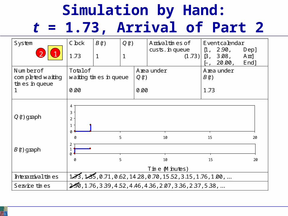
System
Clock 1.73
B(t) 1
Q(t) 1
Arrival times of custs. in queue
(1.73)
Event calendar [1, 2.90, Dep] [3, 3.08, Arr] [–, 20.00, End]
Number of completed waiting times in queue 1
Total of waiting times in queue 0.00
Area under Q(t) 0.00
Area under B(t) 1.73
Q(t) graph B(t) graph
Time (Minutes) Interarrival times 1.73, 1.35, 0.71, 0.62, 14.28, 0.70, 15.52, 3.15, 1.76, 1.00, ...
Service times 2.90, 1.76, 3.39, 4.52, 4.46, 4.36, 2.07, 3.36, 2.37, 5.38, ...
Simulation by Hand: t = 1.73, Arrival of Part 2
0
1
2
3
4
0 5 10 15 20
012
0 5 10 15 20
12
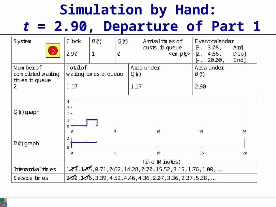
System
Clock 2.90
B(t) 1
Q(t) 0
Arrival times of custs. in queue
<empty>
Event calendar [3, 3.08, Arr] [2, 4.66, Dep] [–, 20.00, End]
Number of completed waiting times in queue 2
Total of waiting times in queue 1.17
Area under Q(t) 1.17
Area under B(t) 2.90
Q(t) graph B(t) graph
Time (Minutes) Interarrival times 1.73, 1.35, 0.71, 0.62, 14.28, 0.70, 15.52, 3.15, 1.76, 1.00, ...
Service times 2.90, 1.76, 3.39, 4.52, 4.46, 4.36, 2.07, 3.36, 2.37, 5.38, ...
Simulation by Hand: t = 2.90, Departure of Part 1
0
1
2
3
4
0 5 10 15 20
012
0 5 10 15 20
2
System
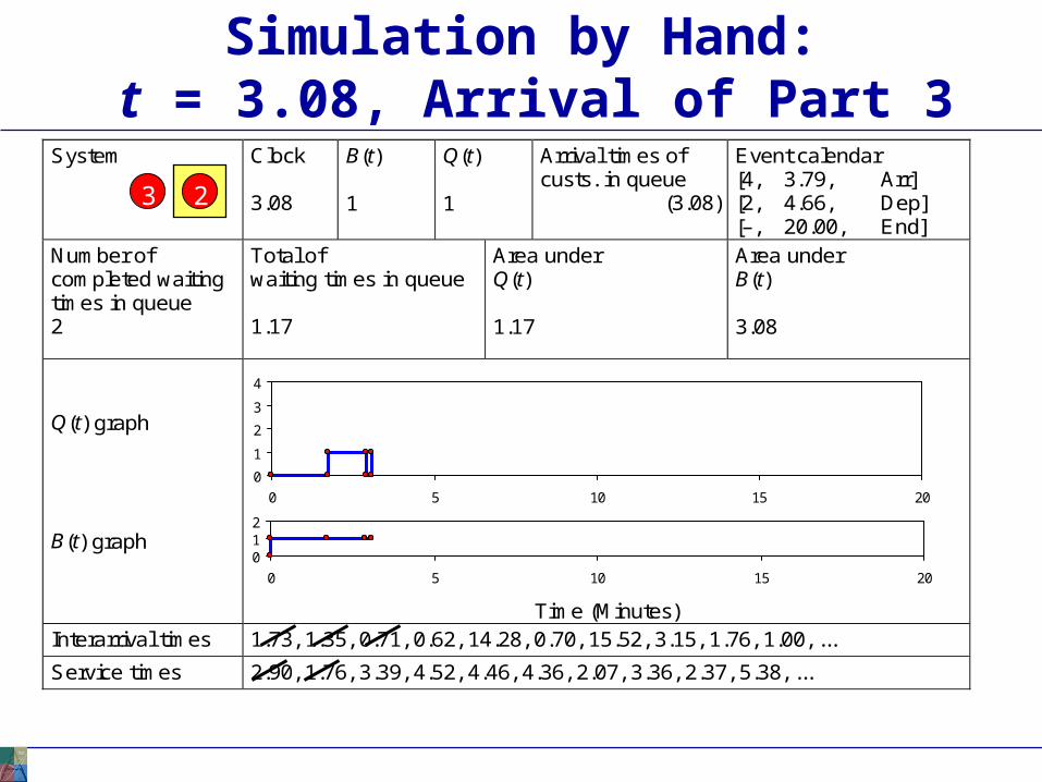
Clock 3.08
B(t) 1
Q(t) 1
Arrival times of custs. in queue
(3.08)
Event calendar [4, 3.79, Arr] [2, 4.66, Dep] [–, 20.00, End]
Number of completed waiting times in queue 2
Total of waiting times in queue 1.17
Area under Q(t) 1.17
Area under B(t) 3.08
Q(t) graph B(t) graph
Time (Minutes) Interarrival times 1.73, 1.35, 0.71, 0.62, 14.28, 0.70, 15.52, 3.15, 1.76, 1.00, ...
Service times 2.90, 1.76, 3.39, 4.52, 4.46, 4.36, 2.07, 3.36, 2.37, 5.38, ...
Simulation by Hand: t = 3.08, Arrival of Part 3
0
1
2
3
4
0 5 10 15 20
012
0 5 10 15 20
23
System
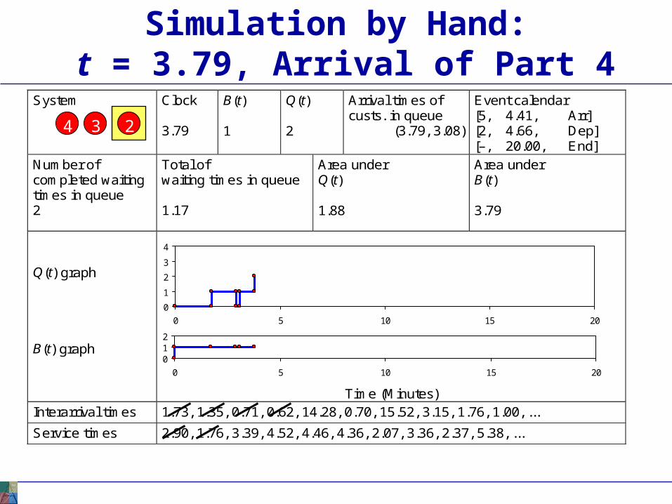
Clock 3.79
B(t) 1
Q(t) 2
Arrival times of custs. in queue
(3.79, 3.08)
Event calendar [5, 4.41, Arr] [2, 4.66, Dep] [–, 20.00, End]
Number of completed waiting times in queue 2
Total of waiting times in queue 1.17
Area under Q(t) 1.88
Area under B(t) 3.79
Q(t) graph B(t) graph
Time (Minutes) Interarrival times 1.73, 1.35, 0.71, 0.62, 14.28, 0.70, 15.52, 3.15, 1.76, 1.00, ...
Service times 2.90, 1.76, 3.39, 4.52, 4.46, 4.36, 2.07, 3.36, 2.37, 5.38, ...
Simulation by Hand: t = 3.79, Arrival of Part 4
0
1
2
3
4
0 5 10 15 20
012
0 5 10 15 20
234
System
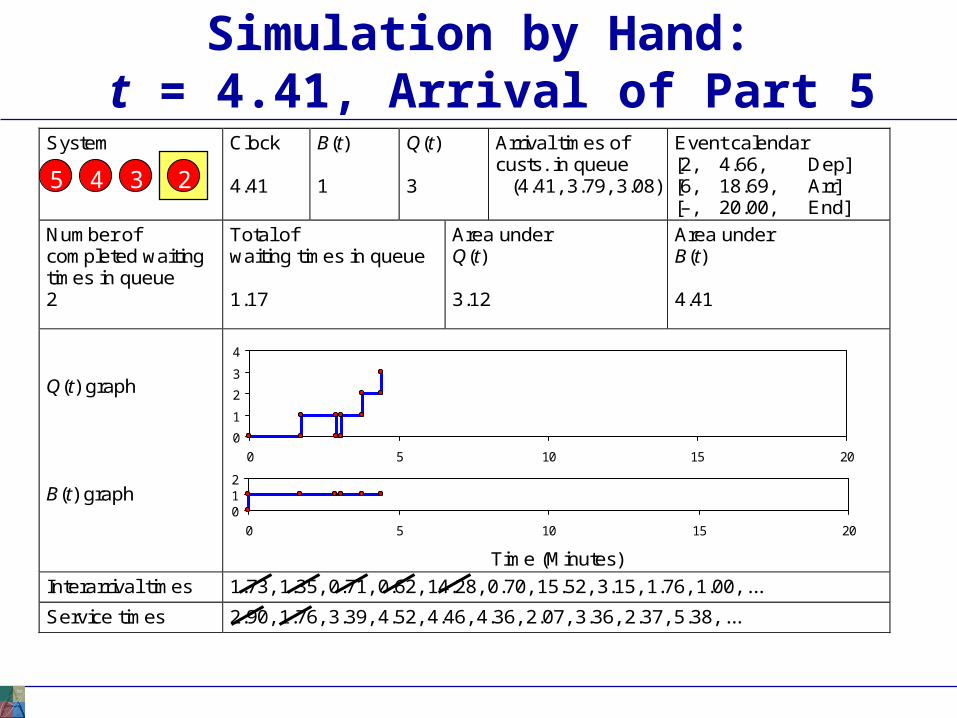
Clock 4.41
B(t) 1
Q(t) 3
Arrival times of custs. in queue
(4.41, 3.79, 3.08)
Event calendar [2, 4.66, Dep] [6, 18.69, Arr] [–, 20.00, End]
Number of completed waiting times in queue 2
Total of waiting times in queue 1.17
Area under Q(t) 3.12
Area under B(t) 4.41
Q(t) graph B(t) graph
Time (Minutes)
Interarrival times 1.73, 1.35, 0.71, 0.62, 14.28, 0.70, 15.52, 3.15, 1.76, 1.00, ...
Service times 2.90, 1.76, 3.39, 4.52, 4.46, 4.36, 2.07, 3.36, 2.37, 5.38, ...
Simulation by Hand: t = 4.41, Arrival of Part 5
0
1
2
3
4
0 5 10 15 20
012
0 5 10 15 20
2345
System
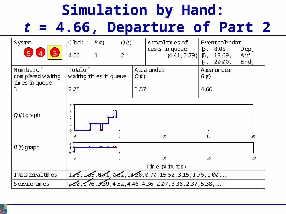
Clock 4.66
B(t) 1
Q(t) 2
Arrival times of custs. in queue
(4.41, 3.79)
Event calendar [3, 8.05, Dep] [6, 18.69, Arr] [–, 20.00, End]
Number of completed waiting times in queue 3
Total of waiting times in queue 2.75
Area under Q(t) 3.87
Area under B(t) 4.66
Q(t) graph B(t) graph
Time (Minutes)
Interarrival times 1.73, 1.35, 0.71, 0.62, 14.28, 0.70, 15.52, 3.15, 1.76, 1.00, ...
Service times 2.90, 1.76, 3.39, 4.52, 4.46, 4.36, 2.07, 3.36, 2.37, 5.38, ...
Simulation by Hand: t = 4.66, Departure of Part 2
0
1
2
3
4
0 5 10 15 20
012
0 5 10 15 20
345
System
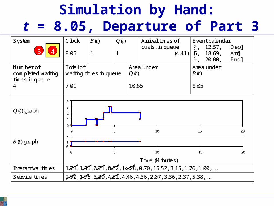
Clock 8.05
B(t) 1
Q(t) 1
Arrival times of custs. in queue
(4.41)
Event calendar [4, 12.57, Dep] [6, 18.69, Arr] [–, 20.00, End]
Number of completed waiting times in queue 4
Total of waiting times in queue 7.01
Area under Q(t) 10.65
Area under B(t) 8.05
Q(t) graph B(t) graph
Time (Minutes)
Interarrival times 1.73, 1.35, 0.71, 0.62, 14.28, 0.70, 15.52, 3.15, 1.76, 1.00, ...
Service times 2.90, 1.76, 3.39, 4.52, 4.46, 4.36, 2.07, 3.36, 2.37, 5.38, ...
Simulation by Hand: t = 8.05, Departure of Part 3
0
1
2
3
4
0 5 10 15 20
012
0 5 10 15 20
45
System
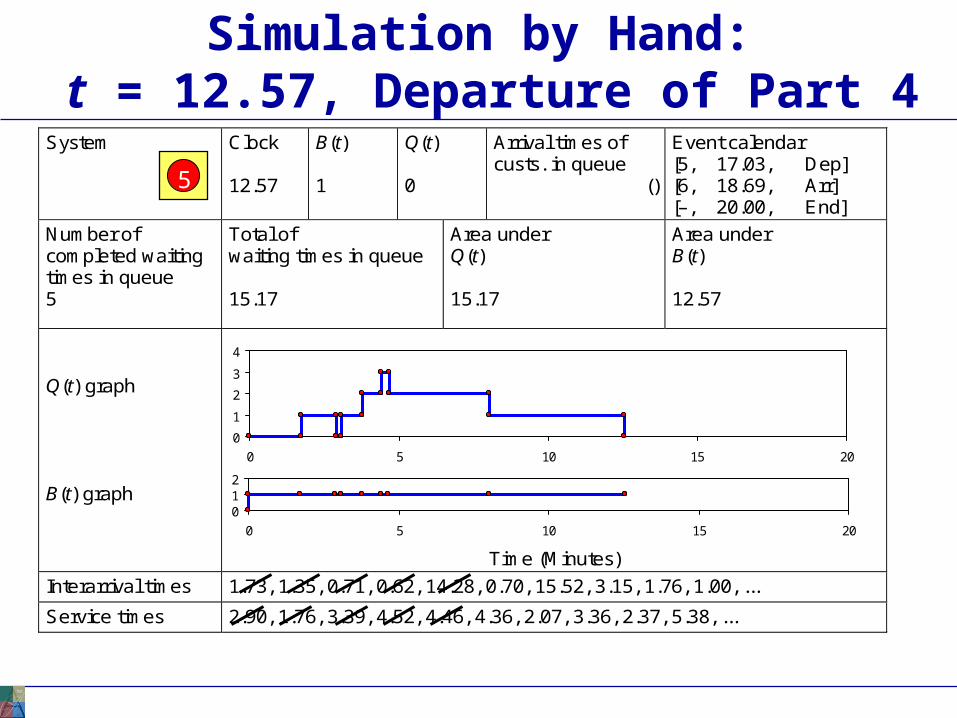
Clock 12.57
B(t) 1
Q(t) 0
Arrival times of custs. in queue
()
Event calendar [5, 17.03, Dep] [6, 18.69, Arr] [–, 20.00, End]
Number of completed waiting times in queue 5
Total of waiting times in queue 15.17
Area under Q(t) 15.17
Area under B(t) 12.57
Q(t) graph B(t) graph
Time (Minutes)
Interarrival times 1.73, 1.35, 0.71, 0.62, 14.28, 0.70, 15.52, 3.15, 1.76, 1.00, ...
Service times 2.90, 1.76, 3.39, 4.52, 4.46, 4.36, 2.07, 3.36, 2.37, 5.38, ...
Simulation by Hand: t = 12.57, Departure of Part 4
0
1
2
3
4
0 5 10 15 20
012
0 5 10 15 20
5
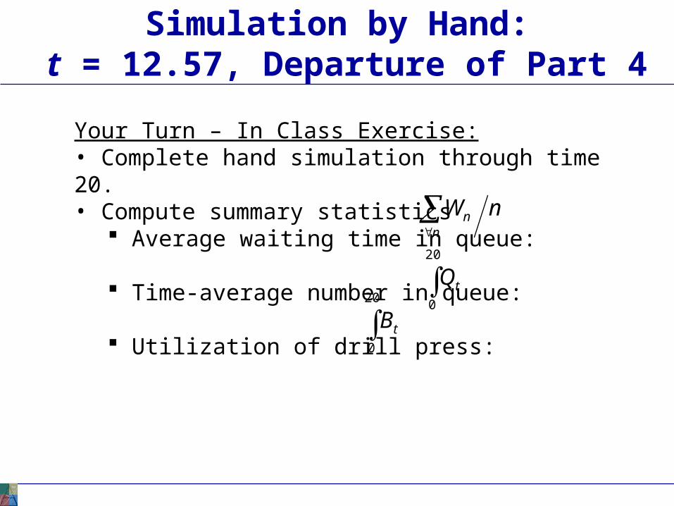
Simulation by Hand: t = 12.57, Departure of Part 4
Your Turn – In Class Exercise:• Complete hand simulation through time 20.• Compute summary statistics
Average waiting time in queue:
Time-average number in queue:
Utilization of drill press:
20
0
tQ
20
0
tB
nWn
n
System
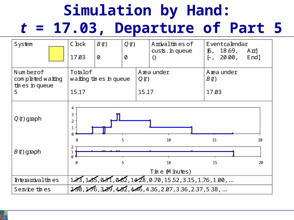
Clock 17.03
B(t) 0
Q(t) 0
Arrival times of custs. in queue ()
Event calendar [6, 18.69, Arr] [–, 20.00, End]
Number of completed waiting times in queue 5
Total of waiting times in queue 15.17
Area under Q(t) 15.17
Area under B(t) 17.03
Q(t) graph B(t) graph
Time (Minutes)
Interarrival times 1.73, 1.35, 0.71, 0.62, 14.28, 0.70, 15.52, 3.15, 1.76, 1.00, ...
Service times 2.90, 1.76, 3.39, 4.52, 4.46, 4.36, 2.07, 3.36, 2.37, 5.38, ...
Simulation by Hand: t = 17.03, Departure of Part 5
0
1
2
3
4
0 5 10 15 20
012
0 5 10 15 20
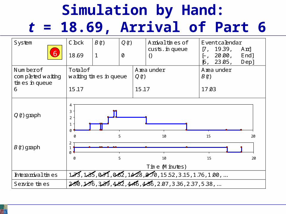
System
Clock 18.69
B(t) 1
Q(t) 0
Arrival times of custs. in queue ()
Event calendar [7, 19.39, Arr] [–, 20.00, End] [6, 23.05, Dep]
Number of completed waiting times in queue 6
Total of waiting times in queue 15.17
Area under Q(t) 15.17
Area under B(t) 17.03
Q(t) graph B(t) graph
Time (Minutes)
Interarrival times 1.73, 1.35, 0.71, 0.62, 14.28, 0.70, 15.52, 3.15, 1.76, 1.00, ...
Service times 2.90, 1.76, 3.39, 4.52, 4.46, 4.36, 2.07, 3.36, 2.37, 5.38, ...
Simulation by Hand: t = 18.69, Arrival of Part 6
0
1
2
3
4
0 5 10 15 20
012
0 5 10 15 20
6
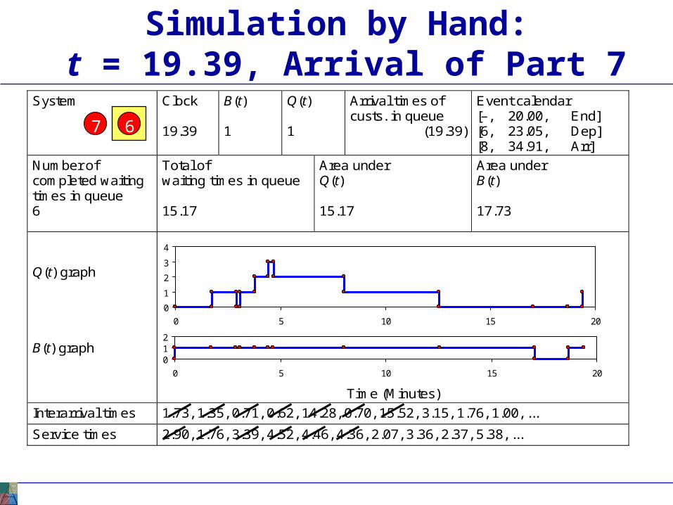
System
Clock 19.39
B(t) 1
Q(t) 1
Arrival times of custs. in queue
(19.39)
Event calendar [–, 20.00, End] [6, 23.05, Dep] [8, 34.91, Arr]
Number of completed waiting times in queue 6
Total of waiting times in queue 15.17
Area under Q(t) 15.17
Area under B(t) 17.73
Q(t) graph B(t) graph
Time (Minutes)
Interarrival times 1.73, 1.35, 0.71, 0.62, 14.28, 0.70, 15.52, 3.15, 1.76, 1.00, ...
Service times 2.90, 1.76, 3.39, 4.52, 4.46, 4.36, 2.07, 3.36, 2.37, 5.38, ...
Simulation by Hand: t = 19.39, Arrival of Part 7
0
1
2
3
4
0 5 10 15 20
012
0 5 10 15 20
67
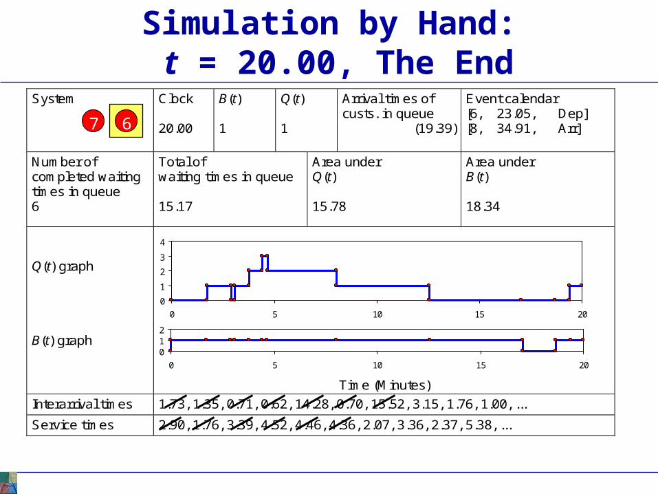
Simulation by Hand: t = 20.00, The End
0
1
2
3
4
0 5 10 15 20
012
0 5 10 15 20
67
System
Clock 20.00
B(t) 1
Q(t) 1
Arrival times of custs. in queue
(19.39)
Event calendar [6, 23.05, Dep] [8, 34.91, Arr]
Number of completed waiting times in queue 6
Total of waiting times in queue 15.17
Area under Q(t) 15.78
Area under B(t) 18.34
Q(t) graph B(t) graph
Time (Minutes)
Interarrival times 1.73, 1.35, 0.71, 0.62, 14.28, 0.70, 15.52, 3.15, 1.76, 1.00, ...
Service times 2.90, 1.76, 3.39, 4.52, 4.46, 4.36, 2.07, 3.36, 2.37, 5.38, ...
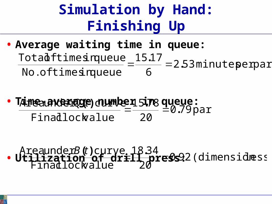
Simulation by Hand:Finishing Up
• Average waiting time in queue:
• Time-average number in queue:
• Utilization of drill press:
part per minutes 53261715
queue in times of No.queue in times of Total
..
part 79020
7815value clock Final
curve under Area.
.)( tQ
less)(dimension 92020
3418value clock Final
curve under Area.
.)( tB
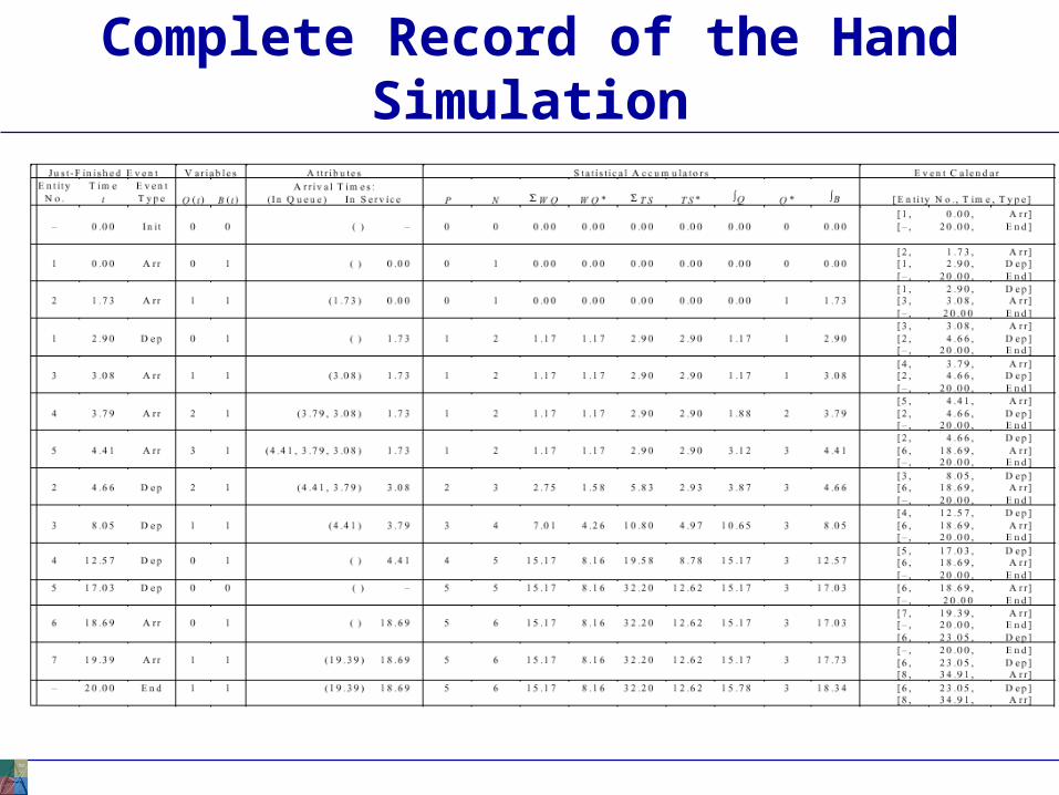
Complete Record of the Hand Simulation
Event-Scheduling Logic via Programming
• Clearly well suited to standard programming language
• Often use “utility” libraries for: List processing Random-number generation Random-variate generation Statistics collection Event-list and clock management Summary and output
• Main program ties it together, executes events in order
Simulation Dynamics: The Process-Interaction World View
• Identify characteristic entities in the system• Multiple copies of entities co-exist, interact,
compete• “Code” is non-procedural• Tell a “story” about what happens to a “typical”
entity• May have many types of entities, “fake” entities
for things like machine breakdowns• Usually requires special simulation software
Underneath, still executed as event-scheduling
• The view normally taken by Arena Arena translates your model description into a program in
the SIMAN simulation language for execution