Embed Size (px)
Citation preview
ETM 607 – Random-Variate Generation
• Inverse-transform technique- Exponential Distribution- Empirical Continuous Distributions- Normal Distribution?
• Discrete Distributions- Empirical- Discrete Uniform- Geometric
• Acceptance-Rejection Technique- Poisson Process- Non-stationary Poisson Process
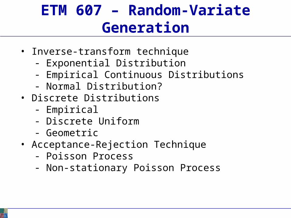
Random-Variate Generation – Chapter 8:
Random-Variate generation is converting from a random number (Ri) to a Random Variable, Xi ~ some distribution.
Inverse transform method:Step 1 – compute cdf of the desired random variable XStep 2 – Set F(X) = R where R is a random number ~U[0,1)Step 3 – Solve F(X) = R for X in terms of R. X = F-1(R).Step 4 – Generate random numbers Ri and compute desired random variates:
Xi = F-1(Ri)
ETM 607 – Random Number and Random Variates
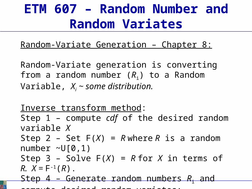
Recall Exponential distribution: is often thought of as the arrival rate, and 1/ as the time between arrivals
Insert figure 5.9
2
1][
1][
0,1
0,0)(
,0
0,)(
XV
XE
xe
xxF
otherwise
xexf
x
x
ETM 607 – Random-Variate Generation
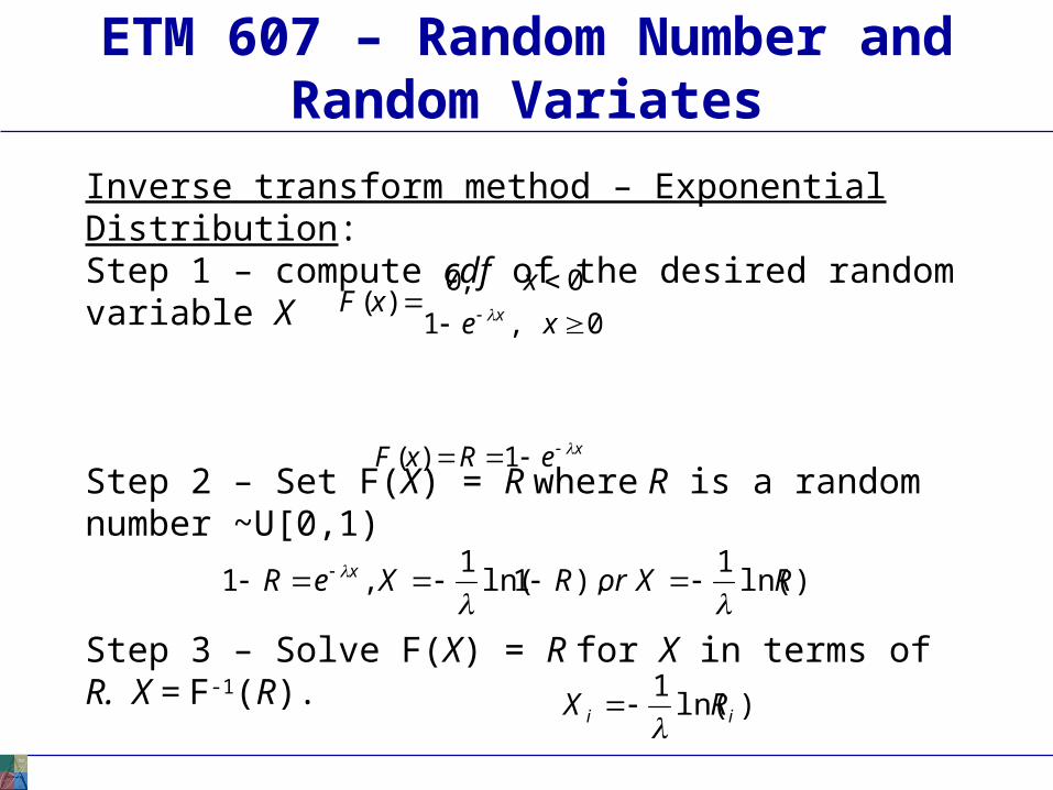
Inverse transform method – Exponential Distribution:Step 1 – compute cdf of the desired random variable X
Step 2 – Set F(X) = R where R is a random number ~U[0,1)
Step 3 – Solve F(X) = R for X in terms of R. X = F-1(R).
Step 4 – Generate random numbers Ri and compute desired random variates:
ETM 607 – Random Number and Random Variates
xeRxF 1)(
)ln(1
),1ln(1
,1 RXorRXeR x
0,1
0,0)(
xe
xxF x
)ln(1
ii RX
Empirical Continuous Distribution:
2 distinct methods:
• Few observations• Many observations
ETM 607 – Random Number and Random Variates
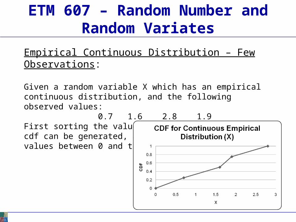
Empirical Continuous Distribution – Few Observations:
Given a random variable X which has an empirical continuous distribution, and the following observed values:
0.7 1.6 2.8 1.9 First sorting the values smallest to largest, a cdf can be generated, assuming X can take on values between 0 and the largest observed value.
ETM 607 – Random Number and Random Variates
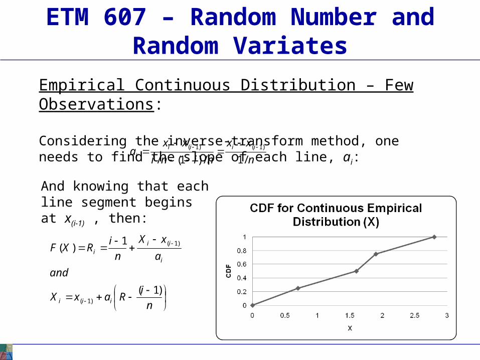
Empirical Continuous Distribution – Few Observations:
Considering the inverse-transform method, one needs to find the slope of each line, ai:
ETM 607 – Random Number and Random Variates
n
xx
nini
xxa iiii
i /1/)1(/)1()1(
And knowing that each line segment begins at x(i-1) , then:
n
iRaxX
and
a
xX
n
iRXF
iii
i
iii
)1(
1)(
)1(
)1(
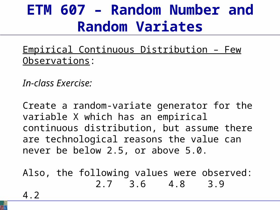
Empirical Continuous Distribution – Few Observations:
In-class Exercise:
Create a random-variate generator for the variable X which has an empirical continuous distribution, but assume there are technological reasons the value can never be below 2.5, or above 5.0.
Also, the following values were observed: 2.7 3.6 4.8 3.9 4.2
What are the values of X, given random numbers: .05, .27, .75, and .98
ETM 607 – Random Number and Random Variates

Empirical Continuous Distribution – Many Observations:
Major difference from “few observations” approach – don’t use 1/n to construct cdf, use n/N, where N is the total number of observations, and n is the observed number of observations for a given interval of the random variable X.
For the slope, ai:
(length of the interval) / (relative frequency of observations within the interval)
Where ci is the value of the cumulative distribution at xi.
See example next slide.
ETM 607 – Random Number and Random Variates
iiii cRaxX )1(

Empirical Continuous Distribution – Many Observations:
Insert example 8.3
ETM 607 – Random Number and Random Variates
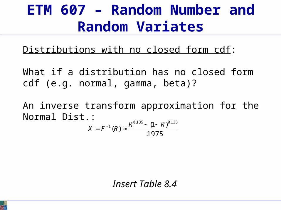
Distributions with no closed form cdf:
What if a distribution has no closed form cdf (e.g. normal, gamma, beta)?
An inverse transform approximation for the Normal Dist.:
Insert Table 8.4
ETM 607 – Random Number and Random Variates
1975.
)1()(
135.0135.01 RR
RFX
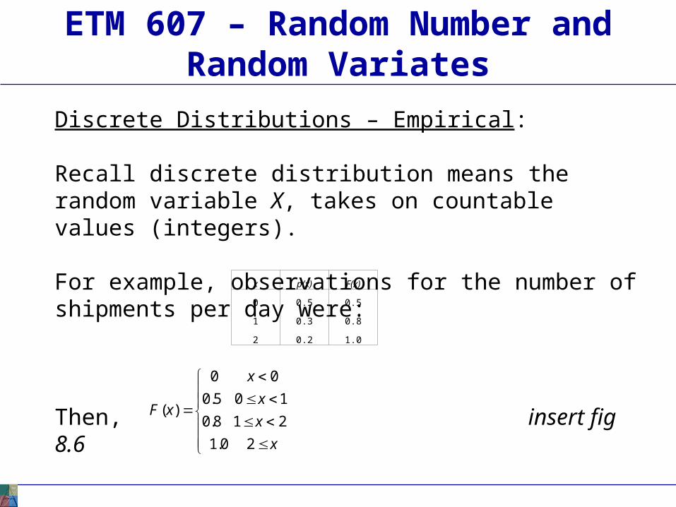
Discrete Distributions – Empirical:
Recall discrete distribution means the random variable X, takes on countable values (integers).
For example, observations for the number of shipments per day were:
Then, insert fig 8.6
ETM 607 – Random Number and Random Variates
x p(x) F(x)
0 0.5 0.5
1 0.3 0.8
2 0.2 1.0
x
x
x
x
xF
20.1
218.0
105.0
00
)(
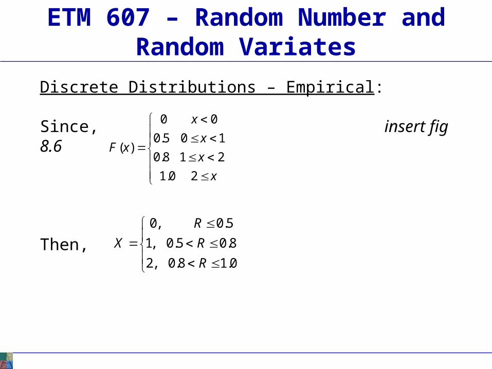
Discrete Distributions – Empirical:
Since, insert fig 8.6
Then,
ETM 607 – Random Number and Random Variates
x
x
x
x
xF
20.1
218.0
105.0
00
)(
0.18.0,2
8.05.0,1
5.0,0
R
R
R
X
Discrete Uniform Distribution:
Inclass Exercise
Consider a random variable X which follows a uniform discrete distribution between and including the numbers [5,10]. Develop an inverse transform for X with respect to R.
ETM 607 – Random Number and Random Variates
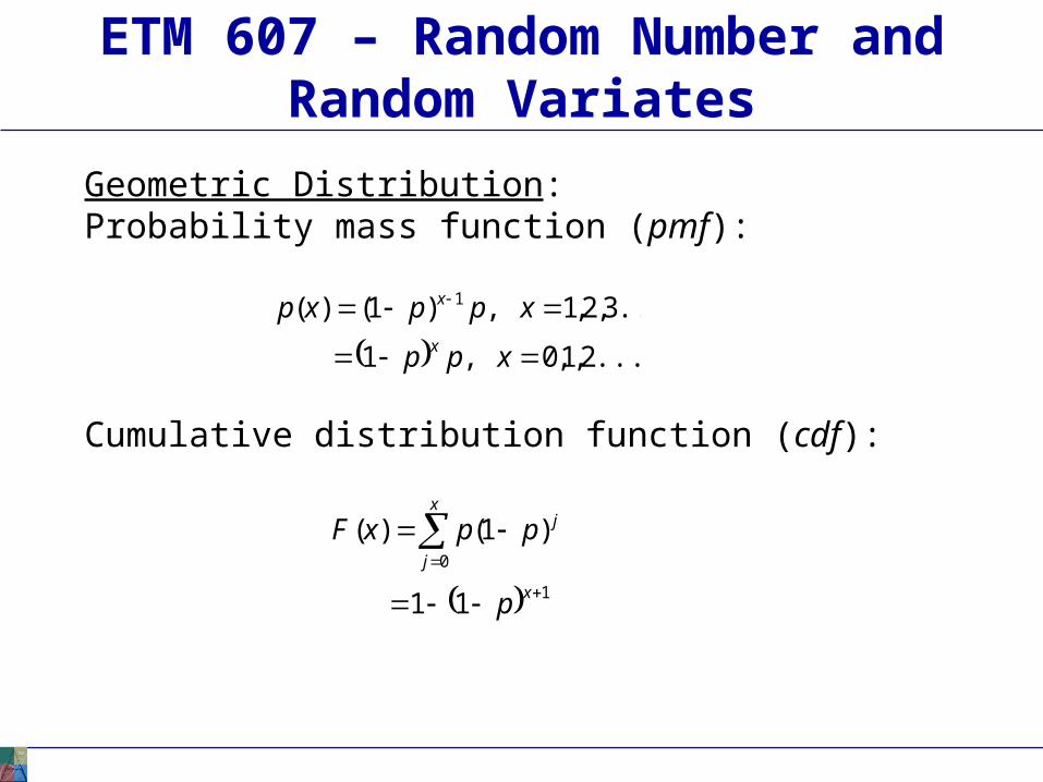
Geometric Distribution:Probability mass function (pmf):
Cumulative distribution function (cdf):
ETM 607 – Random Number and Random Variates
1
0
11
)1()(
x
x
j
j
p
ppxF
...2,1,0,1
...3,2,1,)1()( 1
xpp
xppxpx
x

Geometric Distribution:Knowing the cdf:
Using the inverse transform method:
ETM 607 – Random Number and Random Variates
x
x
pxF
pxF
11)1(
11)( 1
1)1ln(
)1ln(
)1ln(
)1ln(1
)1ln(
)1ln(
)1(1)1(
)1(111
)()1(
1
1
p
RX
p
Rx
p
R
pRp
pRp
xFRxF
xx
xx
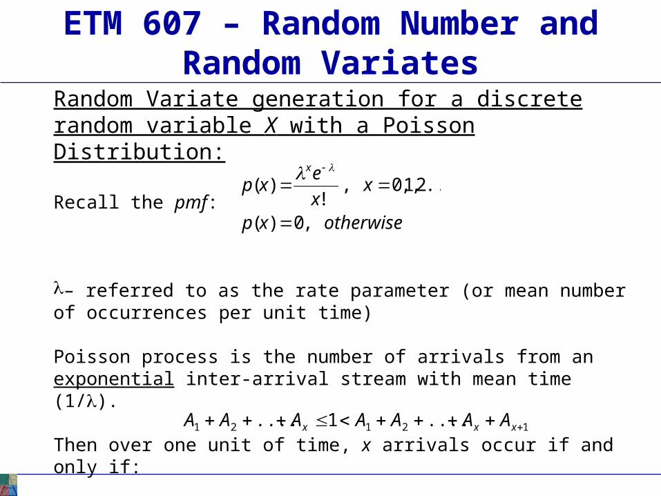
Random Variate generation for a discrete random variable X with a Poisson Distribution:
Recall the pmf:
– referred to as the rate parameter (or mean number of occurrences per unit time)
Poisson process is the number of arrivals from an exponential inter-arrival stream with mean time (1/).
Then over one unit of time, x arrivals occur if and only if:
Where Ai is the inter-arrival time for the ith unit.
ETM 607 – Random Number and Random Variates
otherwisexp
xx
exp
x
,0)(
...2,1,0,!
)(
12121 ....1.... xxx AAAAAAA
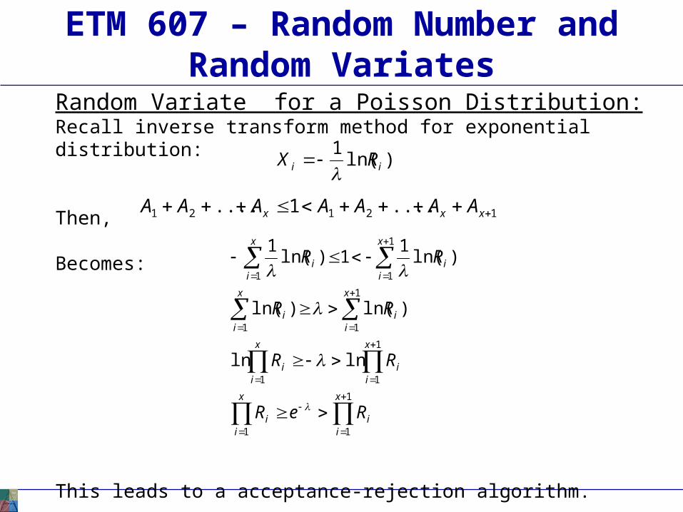
Random Variate for a Poisson Distribution:Recall inverse transform method for exponential distribution:
Then,
Becomes:
This leads to a acceptance-rejection algorithm.
ETM 607 – Random Number and Random Variates
12121 ....1.... xxx AAAAAAA
)ln(1
ii RX
1
11
1
11
1
11
1
11
lnln
)ln()ln(
)ln(1
1)ln(1
x
ii
x
ii
x
ii
x
ii
x
ii
x
ii
x
ii
x
ii
ReR
RR
RR
RR
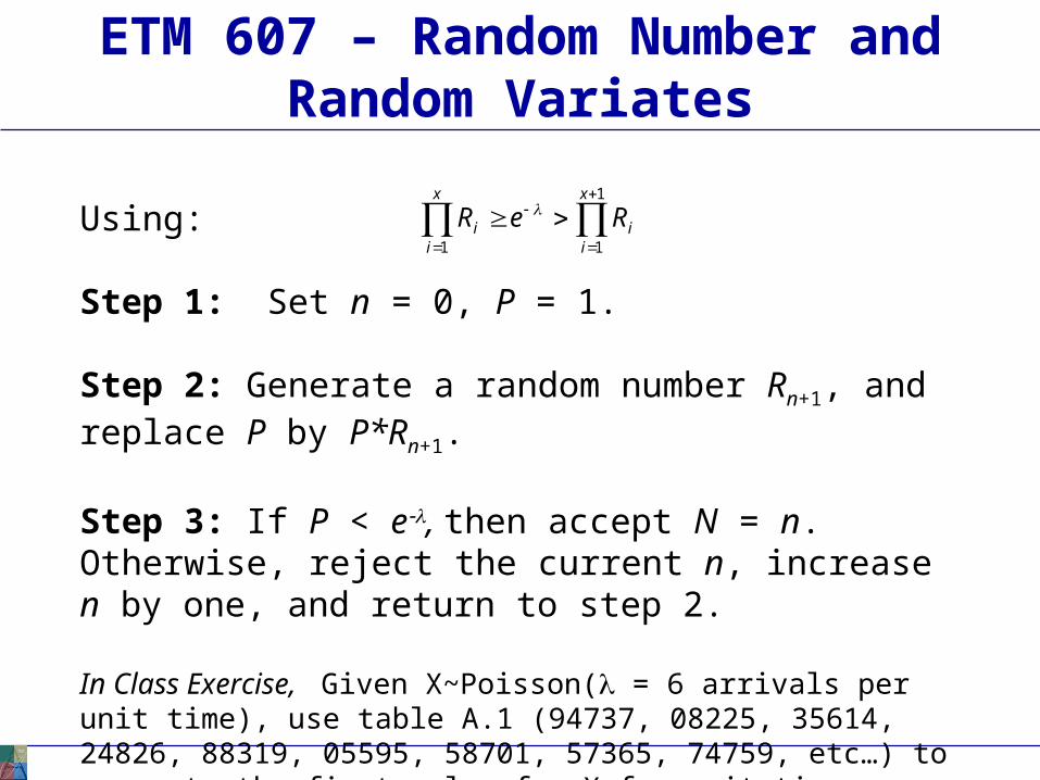
Using:
Step 1: Set n = 0, P = 1.
Step 2: Generate a random number Rn+1, and replace P by P*Rn+1.
Step 3: If P < e, then accept N = n. Otherwise, reject the current n, increase n by one, and return to step 2.
In Class Exercise, Given X~Poisson( = 6 arrivals per unit time), use table A.1 (94737, 08225, 35614, 24826, 88319, 05595, 58701, 57365, 74759, etc…) to generate the first value for X for unit time.
ETM 607 – Random Number and Random Variates
1
11
x
ii
x
ii ReR
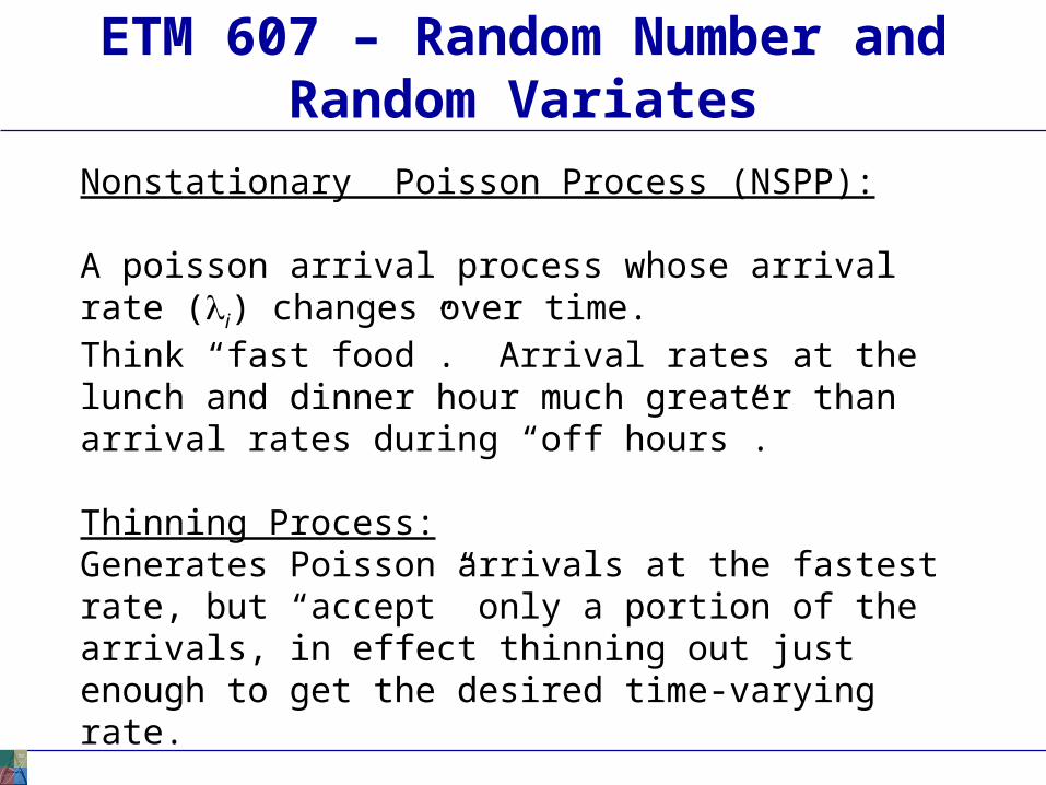
Nonstationary Poisson Process (NSPP):
A poisson arrival process whose arrival rate (i) changes over time.Think “fast food”. Arrival rates at the lunch and dinner hour much greater than arrival rates during “off hours”.
Thinning Process:Generates Poisson arrivals at the fastest rate, but “accept” only a portion of the arrivals, in effect thinning out just enough to get the desired time-varying rate.
ETM 607 – Random Number and Random Variates
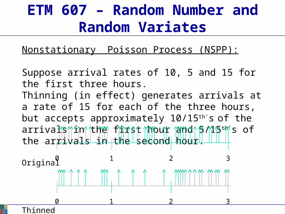
Nonstationary Poisson Process (NSPP):
Suppose arrival rates of 10, 5 and 15 for the first three hours. Thinning (in effect) generates arrivals at a rate of 15 for each of the three hours, but accepts approximately 10/15th’s of the arrivals in the first hour and 5/15th’s of the arrivals in the second hour.
Original
Thinned
ETM 607 – Random Number and Random Variates
0 1 2 3
0 1 2 3
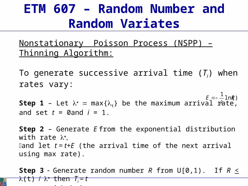
Nonstationary Poisson Process (NSPP) – Thinning Algorithm:
To generate successive arrival time (Ti) when rates vary:
Step 1 – Let max{t} be the maximum arrival rate, and set t = 0and i = 1.
Step 2 – Generate E from the exponential distribution with rate and let t = t+E (the arrival time of the next arrival using max rate).
Step 3Generate random number R from U[0,1). If R < (t)then Ti = t and i = i + 1.
Step 4 – Go to step 2.
ETM 607 – Random Number and Random Variates
)ln(1
RE