ETR 103 - European digital cellular telecommunication system

New

pre

sent

atio

n -

see

His

tory

box

ETSI ETR 103

TECHNICAL October 1993

REPORT

Source: ETSI TC-SMG Reference: GSM 03.30

ICS: 33.060.30

Key words: European digital cellular telecommunications system, Global System for Mobile communications(GSM)

European digital cellular telecommunication system (Phase 2);Radio network planning aspects

(GSM 03.30)

ETSIEuropean Telecommunications Standards Institute

ETSI Secretariat

Postal address: F-06921 Sophia Antipolis CEDEX - FRANCEOffice address: 650 Route des Lucioles - Sophia Antipolis - Valbonne - FRANCEX.400: c=fr, a=atlas, p=etsi, s=secretariat - Internet: [email protected]

Tel.: +33 92 94 42 00 - Fax: +33 93 65 47 16

Copyright Notification: No part may be reproduced except as authorized by written permission. The copyright and theforegoing restriction extend to reproduction in all media.

© European Telecommunications Standards Institute 1993. All rights reserved.

Page 2ETR 103: February 1995 (GSM 03.30 version 4.3.0)

Whilst every care has been taken in the preparation and publication of this document, errors in content,typographical or otherwise, may occur. If you have comments concerning its accuracy, please write to"ETSI Editing and Committee Support Dept." at the address shown on the title page.


Contents

Foreword ...........................................................................................................................................5

1.1. Scope ......................................................................................................................................7

1.2 References...............................................................................................................................7

2. Traffic distributions ....................................................................................................................72.1 Uniform ......................................................................................................................72.2 Non-uniform ................................................................................................................7

3. Cell coverage............................................................................................................................83.1 Location probability .....................................................................................................83.2 Ec/No threshold ..........................................................................................................83.3 RF-budgets ................................................................................................................83.4 Cell ranges .................................................................................................................8

3.4.1 Large cells...............................................................................................83.4.2 Small cells ............................................................................................. 103.4.3 Microcells .............................................................................................. 10

4. Channel re-use........................................................................................................................ 114.1 C/Ic threshold ........................................................................................................... 114.2 Trade-off between Ec/No and C/Ic ............................................................................. 114.3 Adjacent channel suppressions................................................................................... 114.4 Antenna patterns....................................................................................................... 124.5 Antenna heights ........................................................................................................ 124.6 Path loss balance...................................................................................................... 124.7 Cell dimensioning ...................................................................................................... 124.8 Channel allocation ..................................................................................................... 124.9 Frequency hopping.................................................................................................... 134.10 Cells with extra long propagation delay ....................................................................... 13

5. Propagation models................................................................................................................. 135.1 Terrain obstacles ...................................................................................................... 135.2 Environment factors................................................................................................... 135.3 Field strength measurements ..................................................................................... 145.4 Cell adjustments........................................................................................................ 14

6. Glossary................................................................................................................................. 14

7. Bibliography............................................................................................................................ 15

Annex A.1 (class 4): Example of RF-budget for GSM MS handheld RF-output peak power 2 W ............. 16

Annex A.2 (class 2): Example of RF-budget for GSM MS RF-output peak power 8 W ........................... 17

Annex A.3 (DCS1800 classes 1&2): .........Example of RF-budget for DCS 1800 MS RF-output peak power1 W & 250 mW................................................................................................................................. 18

Annex A.4: Example of RF-budget for GSM 900 Class4 (peak power 2 W) in a small cell .................... 19

Annex B: Propagation loss formulas for mobile radiocommunications .............................................. 201. Hata Model [4],[8] ..................................................................................................... 20

1.1 Urban .................................................................................................... 201.2 Suburban............................................................................................... 20


1.3 Rural (Quasi-open) .................................................................................201.4 Rural (Open Area)..................................................................................20

2. COST 231-Hata Model [7] .........................................................................................203. COST 231 Walfish-Ikegami Model [7] .........................................................................21

3.1 Without free line-of-sight between base and mobile (small cells) ................213.2 With a free line-of-sight between base and mobile (Street Canyon) ............21

Annex C: Path Loss vs Cell Radius ................................................................................................22

History .............................................................................................................................................26


Foreword

This ETSI Technical Report (ETR) has been produced by the Special Mobile Group (SMG) TechnicalCommittee (TC) of the European Telecommunications Standards Institute (ETSI).

This ETR Describes the radio network planning aspects within the European digital cellulartelecommunications system (phase 2).

This ETR is an informative document resulting from SMG studies which are related to the European digitalcellular telecommunications system (phase 2). This ETR is used to publish material which is of aninformative nature, relating to the use or the application of ETSs and is not suitable for formal adoption asan ETS.

This ETR correspond to GSM technical specification, GSM 03.30 version 4.2.0.

The specification from which this ETR has been derived was originally based on CEPT documentation,hence the presentation of this ETR may not be entirely in accordance with the ETSI/PNE rules.

Reference is made within this ETR to GSM Technical Specifications (GSM-TS) (NOTE).

NOTE: TC-SMG has produced documents which give the technical specifications for theimplementation of the European digital cellular telecommunications system. Historically,these documents have been identified as GSM Technical Specifications (GSM-TS).These TSs may have subsequently become I-ETSs (Phase 1), or ETSs (Phase 2),whilst others may become ETSI Technical Reports (ETRs). GSM-TSs are, for editorialreasons, still referred to in current GSM ETSs.


Blank page


1.1. Scope

This is a descriptive recommendation to be helpful in cell planning.

1.2 References

This ETR incorporates by dated and undated reference, provisions from other publications. Thesenormative references are cited at the appropriate places in the text and the publications are listedhereafter. For dated references, subsequent amendments to or revisions of any of these publications applyto this ETR only when incorporated in it by amendment or revision. For undated references, the latestedition of the publication referred to applies.

[1] GSM 01.04 (ETR 100): "European digital cellular telecommunication system(Phase 2); Definitions, abbreviations and acronyms".

[2] GSM 05.02 (prETS 300 574): "European digital cellular telecommunicationsystem (Phase 2); Multiplexing and multiple access on the radio path".

[3] GSM 05.05 (prETS 300 577): "European digital cellular telecommunicationsystem (Phase 2); Radio transmission and reception".

[4] GSM 05.08 (prETS 300 578): "European digital cellular telecommunicationsystem (Phase 2); Radio subsystem link control".

[5] CCIR Recommendation 370-5: "VHF and UHF propogation curves for thefrequency range from 30 MHZ to 1000 MHz".

[6] CCIR Report 567-3: "Methods and statistics for estimating field strength valuesin the land mobile services using the frequency range 30 MHz to 1 GHz".

[7] CCIR Report 842: "Spectrum-conserving terestrial frequency assignments forgiven frequency-distance seperations".

[8] CCIR Report 740: "General aspects of cellular systems"

2. Traffic distributions

2.1 Uniform

A uniform traffic distribution can be considered to start with in large cells as an average over the cell area,especially in the country side.

2.2 Non-uniform

A non-uniform traffic distribution is the usual case, especially for urban areas. The traffic peak is usually inthe city centre with local peaks in the suburban centres and motorway junctions.

A bell-shaped area traffic distribution is a good traffic density macro model for cities like London andStockholm. The exponential decay constant is on average 15 km and 7.5 km respectively. However, theexponent varies in different directions depending on how the city is built up. Increasing handheld traffic willsharpen the peak.

Line coverage along communication routes as motorways and streets is a good micro model for car mobiletraffic. For a maturing system an efficient way to increase capacity and quality is to build cells especiallyfor covering these line concentrations with the old area covering cells working as umbrella cells.

Point coverage of shopping centres and traffic terminals is a good micro model for personal handheldtraffic. For a maturing system an efficient way to increase capacity and quality is to build cells on thesepoints as a complement to the old umbrella cells and the new line covering cells for car mobile traffic.


3. Cell coverage

3.1 Location probability

Location probability is a quality criterion for cell coverage. Due to shadowing and fading a cell edge isdefined by adding margins so that the minimum service quality is fulfilled with a certain probability.

For car mobile traffic a usual measure is 90% area coverage per cell, taking into account the minimumsignal-to-noise ratio Ec/No under multipath fading conditions. For lognormal shadowing an area coveragecan be translated into a location probability on cell edge (Jakes, 1974).

For the normal case of urban propagation with a standard deviation of 7 dB and a distance exponential of3.5, 90% area coverage corresponds to about 75% location probability at the cell edge. Furthermore, thelognormal shadow margin in this case will be 5 dB, as described in CEPT Rec. T/R 25-03 and CCIR Rep.740.

3.2 Ec/No threshold

The mobile radio channel is characterized by wideband multipath propagation effects such as delay spreadand Doppler shift as defined in GSM 05.05 Annex 3. The reference signal-to-noise ratio in the modulatingbit rate bandwidth (271 kHz) is Ec/No = 8 dB including 2 dB implementation margin for the GSM system atthe minimum service quality without interference. The Ec/No quality threshold is different for various logicalchannels and propagation conditions as described in GSM 05.05.

3.3 RF-budgets

The RF-link between a base transceiver station (BTS) and a mobile station (MS) including handheld is bestdescribed by an RF-budget as in Annex A which consists of 4 such budgets; A.1 for GSM 900 MS class 4;A.2 for GSM 900 MS class 2, A.3 for DCS 1800 MS classes 1 and 2, and A.4 for GSM 900 class 4 insmall cells.

The antenna gain for the hand portable unit can be set to 0 dBi due to loss in the human body as describedin CCIR Rep. 567. An explicit body loss factor is incorporated in Annex A.3

At 900 MHz, the indoor loss is the field strength decrease when moving into a house on the bottom floor on1.5 m height from the street. The indoor loss near windows ( < 1 m) is typically 12 dB. However, thebuilding loss has been measured by the Finnish PTT to vary between 37 dB and -8 dB with an average of18 dB taken over all floors and buildings (Kajamaa, 1985). See also CCIR Rep. 567.

At 1800 MHz, the indoor loss for large concrete buildings was reported in COST231 TD(90)117 and valuesin the range 12 - 17 dB were measured. Since these buildings are typical of urban areas a value of 15 dBis assumed in annex A.3. In rural areas the buildings tend to be smaller and a 10 dB indoor loss isassumed.

The isotropic power is defined as the RMS value at the terminal of an antenna with 0 dBi gain. A quarter-wave monopole mounted on a suitable earth-plane (car roof) without losses has antenna gain 2 dBi. Anisotropic power of -113 dBm corresponds to a field strength of 23.5 dBuV/m for 925 MHz and 29.3dBuV/m at 1795 MHz, see CEPT Rec. T/R 25-03 and GSM 05.05 Section 5 for formulas. GSM900 BTScan be connected to the same feeders and antennas as analog 900 MHz BTS by diplexers with less than0.5 dB loss.

3.4 Cell ranges

3.4.1 Large cells

In large cells the base station antenna is installed above the maximum height of the surrounding roof tops;the path loss is determined mainly by diffraction and scattering at roof tops in the vicinity of the mobile iethe main rays propagate above the roof tops; the cell radius is minimally 1 km and normally exceeds 3 km.Hata's model and its extension up to 2000 MHz (COST231-Hata model) can be used to calculate the pathloss in such cells (see COST 231 TD (90) 119 Rev 2 and Annex B).


The field strength on 1.5 m reference height outdoor for MS including handheld is a value which inserted inthe curves of CCIR Rep. 567-3 Fig. 2 (Okumura) together with the BTS antenna height and effectiveradiated power (ERP) yields the range and re-use distance for urban areas (Section 5.2).

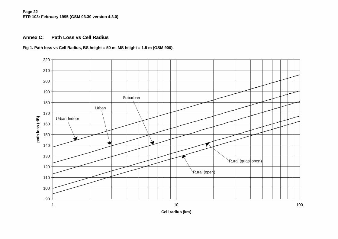
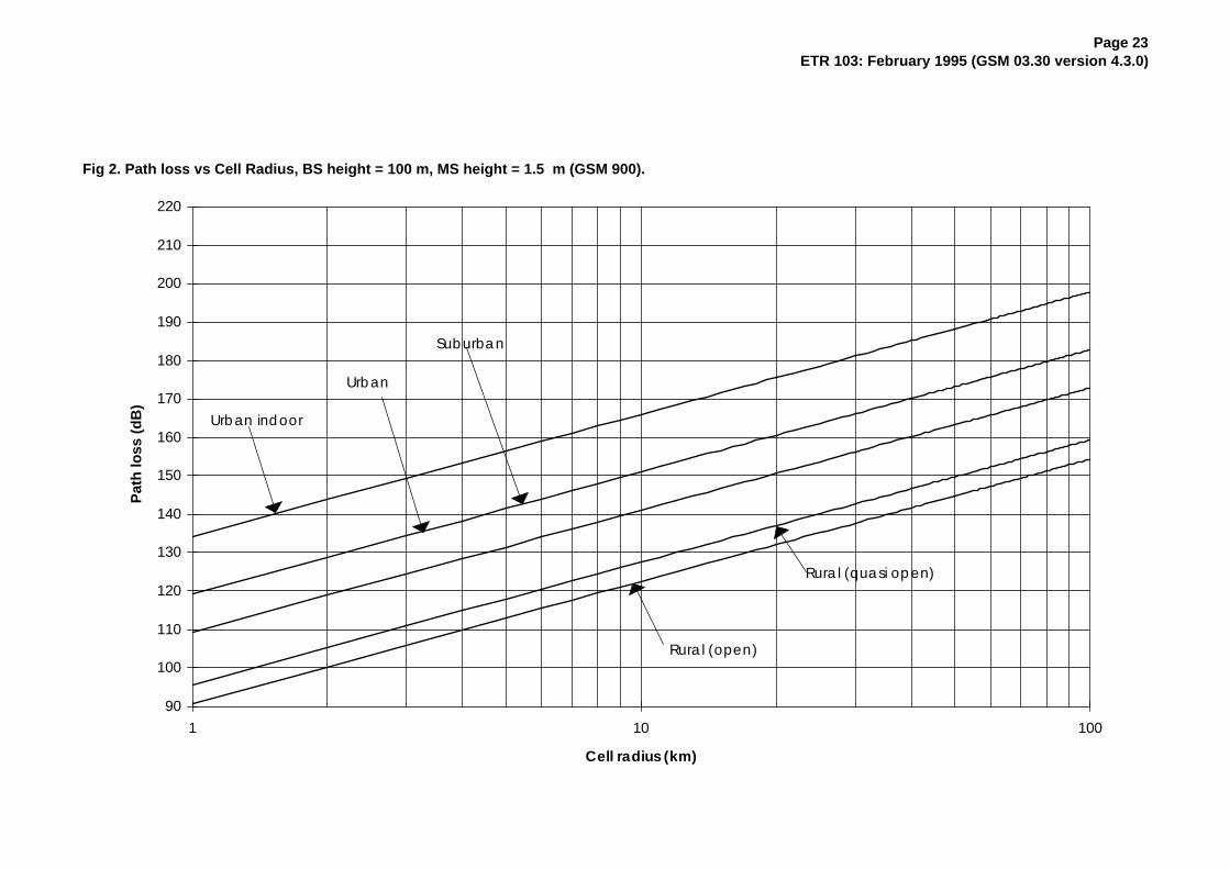
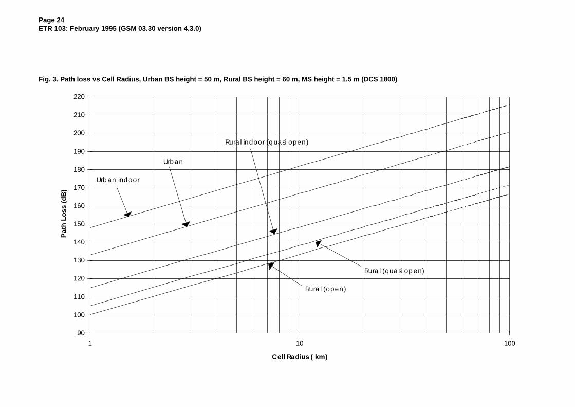
The cell range can also be calculated by putting the maximum allowed path loss between isotropicantennas into the Figures 1 to 3 of Annex C. The same path loss can be found in the RF-budgets in AnnexA. The figures 1 and 2 (GSM900) in Annex C are based on Hata's propagation model which fits Okumura'sexperimental curves up to 1500 MHz and figure 3 (DCS 1800) is based on COST231-Hata modelaccording to COST 231 TD (90) 119 Rev 2.

The example RF-budget shown in Annex A.1 for a GSM900 MS handheld output power 2 W yields aboutdouble the range outdoors compared with indoors. This means that if the cells are dimensioned forhandhelds with indoor loss 10 dB, the outdoor coverage for MS will be interference limited, see Section4.2. Still more extreme coverage can be found over open flat land of 12 km as compared with 3 km inurban areas outdoor to the same cell site.

For GSM 900 the Max EIRP of 50 W matches MS class 2 of max peak output power 8 W, see Annex A.2.

An example RF budget for DCS1800 is shown in Annex A.3. Range predictions are given for 1 W and 250mW DCS1800 MS with BTS powers which balance the up- and down- links.

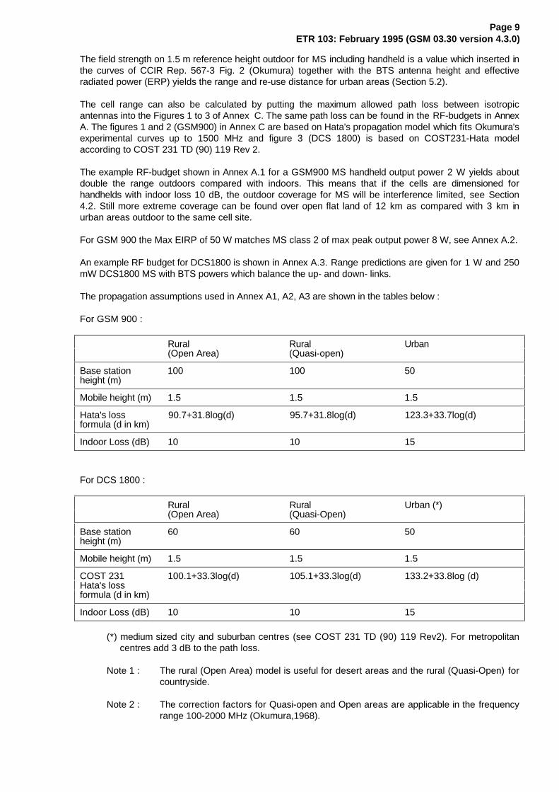
The propagation assumptions used in Annex A1, A2, A3 are shown in the tables below :

For GSM 900 :

Rural Rural Urban(Open Area) (Quasi-open)

Base station 100 100 50height (m)

Mobile height (m) 1.5 1.5 1.5

Hata's loss 90.7+31.8log(d) 95.7+31.8log(d) 123.3+33.7log(d)formula (d in km)

Indoor Loss (dB) 10 10 15

For DCS 1800 :

Rural Rural Urban (*)(Open Area) (Quasi-Open)

Base station 60 60 50height (m)

Mobile height (m) 1.5 1.5 1.5

COST 231 100.1+33.3log(d) 105.1+33.3log(d) 133.2+33.8log (d)Hata's lossformula (d in km)

Indoor Loss (dB) 10 10 15

(*) medium sized city and suburban centres (see COST 231 TD (90) 119 Rev2). For metropolitancentres add 3 dB to the path loss.

Note 1 : The rural (Open Area) model is useful for desert areas and the rural (Quasi-Open) forcountryside.

Note 2 : The correction factors for Quasi-open and Open areas are applicable in the frequencyrange 100-2000 MHz (Okumura,1968).


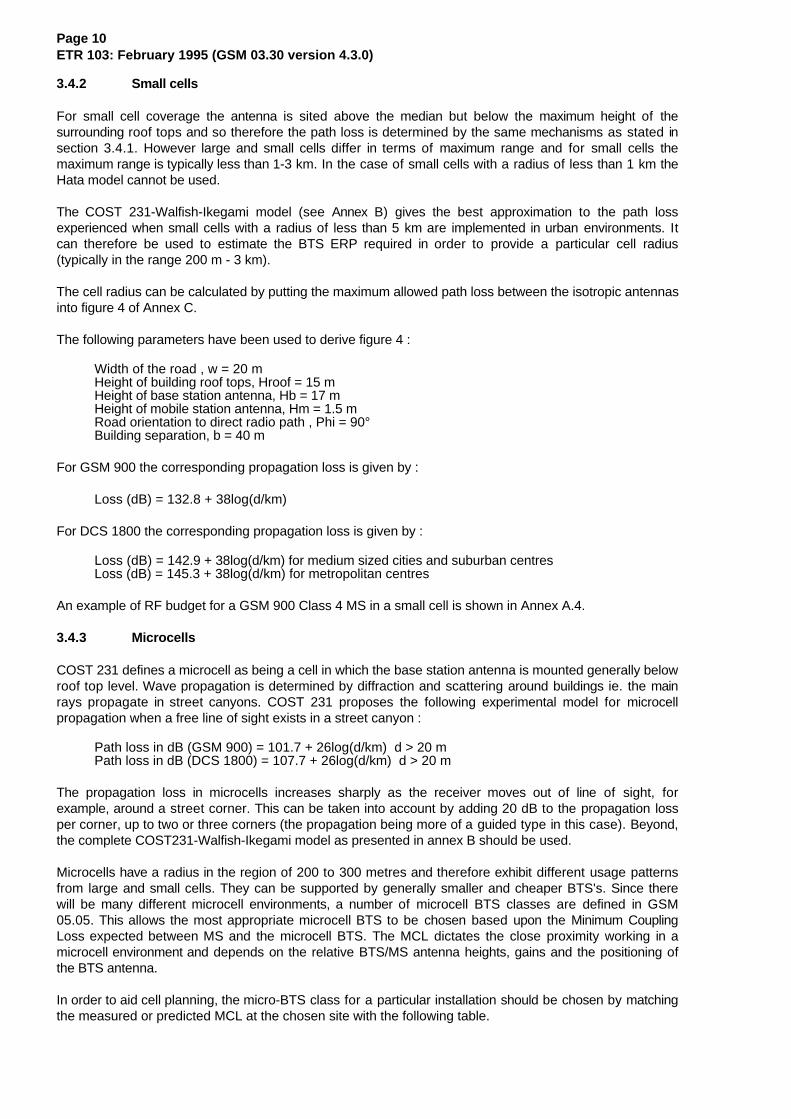
3.4.2 Small cells

For small cell coverage the antenna is sited above the median but below the maximum height of thesurrounding roof tops and so therefore the path loss is determined by the same mechanisms as stated insection 3.4.1. However large and small cells differ in terms of maximum range and for small cells themaximum range is typically less than 1-3 km. In the case of small cells with a radius of less than 1 km theHata model cannot be used.

The COST 231-Walfish-Ikegami model (see Annex B) gives the best approximation to the path lossexperienced when small cells with a radius of less than 5 km are implemented in urban environments. Itcan therefore be used to estimate the BTS ERP required in order to provide a particular cell radius(typically in the range 200 m - 3 km).

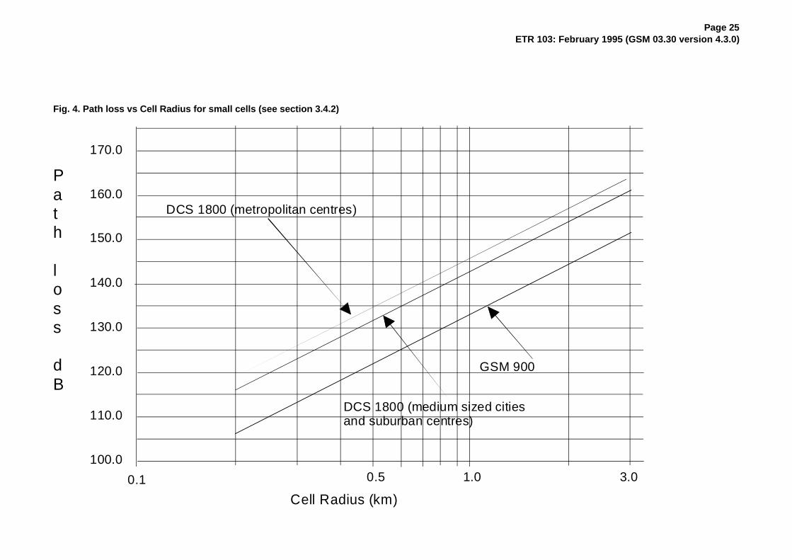
The cell radius can be calculated by putting the maximum allowed path loss between the isotropic antennasinto figure 4 of Annex C.

The following parameters have been used to derive figure 4 :

Width of the road , w = 20 mHeight of building roof tops, Hroof = 15 mHeight of base station antenna, Hb = 17 mHeight of mobile station antenna, Hm = 1.5 mRoad orientation to direct radio path , Phi = 90°Building separation, b = 40 m

For GSM 900 the corresponding propagation loss is given by :

Loss (dB) = 132.8 + 38log(d/km)

For DCS 1800 the corresponding propagation loss is given by :

Loss (dB) = 142.9 + 38log(d/km) for medium sized cities and suburban centresLoss (dB) = 145.3 + 38log(d/km) for metropolitan centres

An example of RF budget for a GSM 900 Class 4 MS in a small cell is shown in Annex A.4.

3.4.3 Microcells

COST 231 defines a microcell as being a cell in which the base station antenna is mounted generally belowroof top level. Wave propagation is determined by diffraction and scattering around buildings ie. the mainrays propagate in street canyons. COST 231 proposes the following experimental model for microcellpropagation when a free line of sight exists in a street canyon :

Path loss in dB (GSM 900) = 101.7 + 26log(d/km) d > 20 mPath loss in dB (DCS 1800) = 107.7 + 26log(d/km) d > 20 m

The propagation loss in microcells increases sharply as the receiver moves out of line of sight, forexample, around a street corner. This can be taken into account by adding 20 dB to the propagation lossper corner, up to two or three corners (the propagation being more of a guided type in this case). Beyond,the complete COST231-Walfish-Ikegami model as presented in annex B should be used.

Microcells have a radius in the region of 200 to 300 metres and therefore exhibit different usage patternsfrom large and small cells. They can be supported by generally smaller and cheaper BTS's. Since therewill be many different microcell environments, a number of microcell BTS classes are defined in GSM05.05. This allows the most appropriate microcell BTS to be chosen based upon the Minimum CouplingLoss expected between MS and the microcell BTS. The MCL dictates the close proximity working in amicrocell environment and depends on the relative BTS/MS antenna heights, gains and the positioning ofthe BTS antenna.

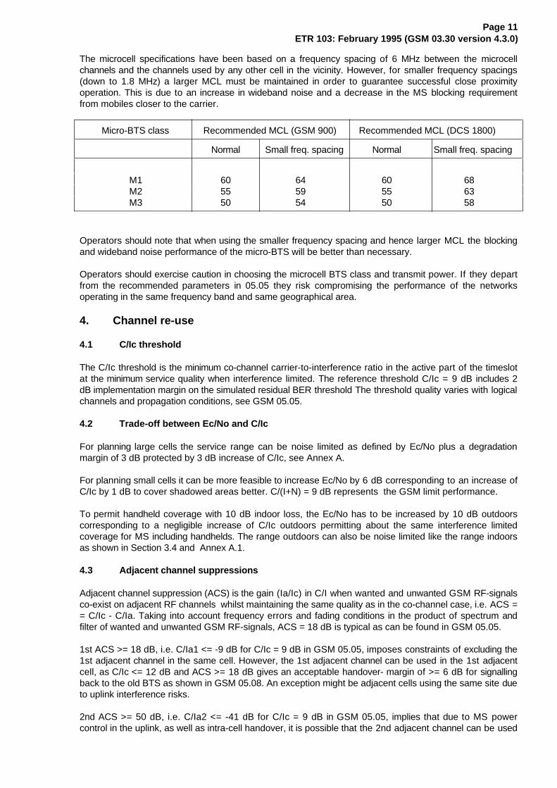
In order to aid cell planning, the micro-BTS class for a particular installation should be chosen by matchingthe measured or predicted MCL at the chosen site with the following table.


The microcell specifications have been based on a frequency spacing of 6 MHz between the microcellchannels and the channels used by any other cell in the vicinity. However, for smaller frequency spacings(down to 1.8 MHz) a larger MCL must be maintained in order to guarantee successful close proximityoperation. This is due to an increase in wideband noise and a decrease in the MS blocking requirementfrom mobiles closer to the carrier.

Micro-BTS class Recommended MCL (GSM 900) Recommended MCL (DCS 1800)

Normal Small freq. spacing Normal Small freq. spacing

M1 60 64 60 68M2 55 59 55 63M3 50 54 50 58

Operators should note that when using the smaller frequency spacing and hence larger MCL the blockingand wideband noise performance of the micro-BTS will be better than necessary.

Operators should exercise caution in choosing the microcell BTS class and transmit power. If they departfrom the recommended parameters in 05.05 they risk compromising the performance of the networksoperating in the same frequency band and same geographical area.

4. Channel re-use

4.1 C/Ic threshold

The C/Ic threshold is the minimum co-channel carrier-to-interference ratio in the active part of the timeslotat the minimum service quality when interference limited. The reference threshold C/Ic = 9 dB includes 2dB implementation margin on the simulated residual BER threshold The threshold quality varies with logicalchannels and propagation conditions, see GSM 05.05.

4.2 Trade-off between Ec/No and C/Ic

For planning large cells the service range can be noise limited as defined by Ec/No plus a degradationmargin of 3 dB protected by 3 dB increase of C/Ic, see Annex A.

For planning small cells it can be more feasible to increase Ec/No by 6 dB corresponding to an increase ofC/Ic by 1 dB to cover shadowed areas better. C/(I+N) = 9 dB represents the GSM limit performance.

To permit handheld coverage with 10 dB indoor loss, the Ec/No has to be increased by 10 dB outdoorscorresponding to a negligible increase of C/Ic outdoors permitting about the same interference limitedcoverage for MS including handhelds. The range outdoors can also be noise limited like the range indoorsas shown in Section 3.4 and Annex A.1.

4.3 Adjacent channel suppressions

Adjacent channel suppression (ACS) is the gain (Ia/Ic) in C/I when wanted and unwanted GSM RF-signalsco-exist on adjacent RF channels whilst maintaining the same quality as in the co-channel case, i.e. ACS == C/Ic - C/Ia. Taking into account frequency errors and fading conditions in the product of spectrum andfilter of wanted and unwanted GSM RF-signals, ACS = 18 dB is typical as can be found in GSM 05.05.

1st ACS >= 18 dB, i.e. C/Ia1 <= -9 dB for C/Ic = 9 dB in GSM 05.05, imposes constraints of excluding the1st adjacent channel in the same cell. However, the 1st adjacent channel can be used in the 1st adjacentcell, as C/Ic <= 12 dB and ACS >= 18 dB gives an acceptable handover- margin of >= 6 dB for signallingback to the old BTS as shown in GSM 05.08. An exception might be adjacent cells using the same site dueto uplink interference risks.

2nd ACS >= 50 dB, i.e. C/Ia2 <= -41 dB for C/Ic = 9 dB in GSM 05.05, implies that due to MS powercontrol in the uplink, as well as intra-cell handover, it is possible that the 2nd adjacent channel can be used


in the same cell. Switching transients are not interfering due to synchronised transmission and reception ofbursts at co-located BTS.

4.4 Antenna patterns

Antenna patterns including surrounding masts, buildings, and terrain measured on ca 1 km distance willalways look directional, even if the original antenna was non-directional. In order to achieve a front-to-back ratio F/B of greater than 20 dB from an antenna with an ideal F/B > 25 dB, backscattering from themain lobe must be suppressed by using an antenna height of at least 10 m above forward obstacles in ca0.5 km. In order to achieve an omni-directional pattern with as few nulls as possible, the ideal non-directional antenna must be isolated from the mast by a suitable reflector. The nulls from mast scatteringare usually in different angles for the duplex frequencies and should be avoided because of creating pathloss imbalance.

The main lobe antenna gains are typically 12-18 dBi for BTS, and 2-5 dBi for MS. Note that a dipole hasthe gain 0 dBd = 2 dBi.

4.5 Antenna heights

The height gain under Rayleigh fading conditions is approximately 6 dB by doubling the BTS antennaheight. The same height gain for MS and handheld from reference height 1.5 m to 10 m is about 9 dB,which is the correction needed for using CCIR Rec. 370.

4.6 Path loss balance

Path loss balance on uplink and downlink is important for two-way communication near the cell edge.Speech as well as data transmission is dimensioned for equal quality in both directions. Balance is onlyachieved for a certain power class (Section 3.4).

Path loss imbalance is taken care of in cell selection in idle mode and in the handover decision algorithmsas found in GSM 05.08. However, a cell dimensioned for 8 W MS (GSM 900 class 2) can more or lessgain balance for 2 W MS handheld (GSM 900 class 4) by implementing antenna diversity reception on theBTS.

4.7 Cell dimensioning

Cell dimensioning for uniform traffic distribution is optimised by at any time using the same number ofchannels and the same coverage area per cell.

Cell dimensioning for non-uniform traffic distribution is optimised by at any time using the same number ofchannels but changing the cell coverage area so that the traffic carried per cell is kept constant with thetraffic density. Keeping the path loss balance by directional antennas pointing outwards from the trafficpeaks the effective radiated power (ERP) per BTS can be increased rapidly out-wards. In order to makethe inner cells really small the height gain can be decreased and the antenna gain can be made smaller oreven negative in dB by increasing the feeder loss but keeping the antenna front-to-back ratio constant(Section 4.4).

4.8 Channel allocation

Channel allocation is normally made on an FDMA basis. However, in synchronised networks channelallocation can be made on a TDMA basis. Note that a BCCH RF channel must always be fully allocated toone cell.

Channel allocation for uniform traffic distribution preferably follows one of the well known re-use clustersdepending on C/I-distribution, e.g. a 9-cell cluster (3-cell 3-site repeat pattern) using 9 RF channel groupsor cell allocations (CAs), (Stjernvall, 1985).

Channel allocation for non-uniform traffic distribution preferably follows a vortex from a BTS concentrationon the traffic centre, if a bell-shaped area traffic model holds. In real life the traffic distribution is morecomplicated with also line and point traffic. In this case the cell areas will be rather different for various


BTS locations from city centre. The channel allocation can be optimised by using graph colouring heuristicsas described in CCIR Rep. 842.

Base transceiver station identity code (BSIC) allocation is done so that maximum re-use distance percarrier is achieved in order to exclude co-channel ambiguity.

Frequency coordination between countries is a matter of negotiations between countries as described inCEPT Rec.T/R 25-04. Co-channel and 200 kHz adjacent channels need to be considered between PLMNsand other services as stated in GSM 05.05.

Frequency sharing between GSM countries is regulated in CEPT Rec. T/R 20-08 concerning frequencyplanning and frequency coordination for the GSM service.

4.9 Frequency hopping

Frequency hopping (FH) can easily be implemented if the re-use is based on RF channel groups (CAs). Itis also possible to change allocation by demand as described in GSM 05.02.

In synchronised networks the synchronisation bursts (SB) on the BCCH will occur at the same time ondifferent BTS. This will increase the time to decode the BSIC of adjacent BTS, see GSM 05.08. TheSACCH on the TCH or SDCCH will also occur at the same time on different BTS. This will decrease theadvantage of discontinuous transmission (DTX). In order to avoid this an offset in the time base (FN)between BTS may be used.

If channel allocation is made on a TDMA basis and frequency hopping is used, the same hop sequencemust be used on all BTS. Therefore the same time base and the same hopping sequence number (HSN)shall be used.

4.10 Cells with extra long propagation delay

Cells with anticipated traffic with ranges more than 35 km corresponding to maximum MS timing advancecan work properly if the timeslot after the CCCH is barred corresponding to a maximum total range of 120km. From BTS timing measurements an MS with longer range than 35 km are guarded by one extratimeslot. This holds for all kinds of channels.

5. Propagation models

5.1 Terrain obstacles

Terrain obstacles introduce diffraction loss, which can be estimated from the path profile betweentransmitter and receiver antennas. The profile can preferably be derived from a digital topographic databank delivered from the national map survey or from a land resource satellite system, e.g. Spot. Theresolution is usually 500*500 m2 down to 50*50 m2 in side and 20 m down to 5 m in height. This resolutionis not sufficient to describe the situation in cities for microcells, where streets and buildings must berecognised.

5.2 Environment factors

Environment factors for the nearest 200 m radius from the mobile play an important role in both the 900MHz and 1800 MHz bands. For the Nordic cellular planning for NMT there is taken into account 10categories for land, urban and wood. Further studies are done within COST 231.

Coarse estimations of cell coverage can be done on pocket computers with programs adding theseenvironment factors to propagation curves of CCIR Rec. 370-5 Fig. 9 and CCIR Rep. 567-3 Fig. 2(Okumura, 1968).


5.3 Field strength measurements

Field strength measurements of the local mean of the lognormal distribution are preferably done by digitalaveraging over the typical Rayleigh fading. It can be shown that the local average power can be estimatedover 20 to 40 wavelengths with at least 36 uncorrelated samples within 1 dB error for 90% confidence(Lee, 1985).

5.4 Cell adjustments

Cell adjustments from field strength measurements of coverage and re-use are recommended after coarsepredictions have been done. Field strength measurements of rms values can be performed with anuncertainty of 3.5 dB due to sampling and different propagation between Rayleigh fading and line-of-sight.Predictions can reasonably be done with an uncertainty of about 10 dB. Therefore cell adjustments arepreferably done from field strength measurements by changing BTS output power, ERP, and antennapattern in direction and shape.

6. Glossary

ACS Adjacent Channel Suppression (Section 4.3)BCCH Broadcast Control Channel (Section 4.8)BTS Base Transceiver Station (Section 3.3)BSIC Base Transceiver Station Identity Code (Section 4.8)CA Cell Allocation of radio frequency channels (Section 4.8)CCCH Common Control Channel (Section 4.10)COST European Cooperation in the field of Scientific and Technical ResearchDTX Discontinuous Transmission (Section 4.9)Ec/No Signal-to-Noise ratio in modulating bit rate bandwidth (Section3.2)FH Frequency Hopping (Section 4.9)FN TDMA Frame Number (Section 4.9)F/B Front-to-Back ratio (Section 4.4)HSN Hopping Sequence Number (Section 4.9)MS Mobile Station (Section 3.3)PLMN Public Land Mobile NetworkPs Location (site) Probability (Section 3.1)SACCH Slow Associated Control Channel (Section 4.9)SB Synchronisation Burst (Section 4.9)SDCCH Stand-alone Dedicated Control Channel (Section 4.9)TCH Traffic Channel (Section 4.9)


7. Bibliography

0 CEPT Recommendation T/R 20-08 Frequency planning and frequency coordination for the GSMservice;

CEPT Recommendation T/R 25-03 Coordination of frequencies for the land mobile service in the 80,160 and 460 MHz bands and the methods to be used for assessing interference;

CEPT Recommendation T/R 25-04 Coordination in frontier regions of frequencies for the land mobileservice in the bands between 862 and 960 MHz;

CEPT Liaison office, P.O.Box 1283, CH-3001 Berne.

1 Jakes, W.C., Jr.(Ed.) (1974) Microwave mobile communications. John Wiley, New York, NY, USA.

2 Kajamaa, Timo (1985) 900 MHz propagation measurements in Finland in 1983-85 (PTT Report27.8.1985.) Proc NRS 86, Nordic Radio Symposium, ISBN 91-7056-072-2.

3 Lee, W.C.Y. (Feb., 1985) Estimate of local average power of a mobile radio signal. IEEE Trans.Vehic. Tech., Vol. VT-34, 1.

4 Okumura, Y. et al (Sep.-Oct., 1968) Field strength and its variability in VHF and UHF land-mobileradio service. Rev. Elec. Comm. Lab., NTT, Vol. 16, 9-10.

5 Stjernvall, J-E (Feb. 1985) Calculation of capacity and co-channel interference in a cellular system.Nordic Seminar on Digital Land Mobile Radio Communication (DMR I), Espoo, Finland.

6 A.M.D. Turkmani, J.D. Parsons and A.F. de Toledo "Radio Propagation into Buildings at 1.8 GHz".COST 231 TD (90) 117

7 COST 231 "Urban transmission loss models for mobile radio in the 900- and 1800- MHz bands(Revision 2)" COST 231 TD (90) 119 Rev 2.

8 Hata, M. (1980) Empirical Formula for Propagation Loss in Land Mobile Radio Services, IEEETrans. on Vehicular Technology VT-29.


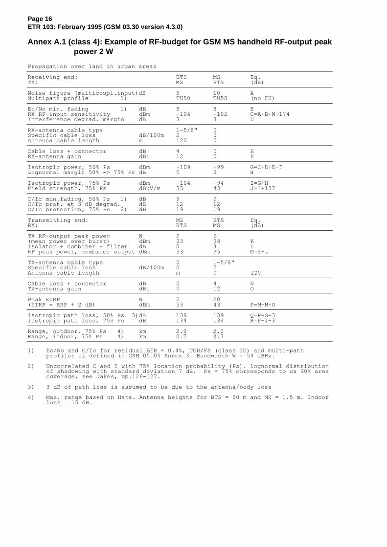
Annex A.1 (class 4): Example of RF-budget for GSM MS handheld RF-output peakpower 2 W

Propagation over land in urban areas

Receiving end: BTS MS Eq.TX: MS BTS (dB)

Noise figure (multicoupl.input)dB 8 10 AMultipath profile 1) TU50 TU50 (no FH)

Ec/No min. fading 1) dB 8 8 BRX RF-input sensitivity dBm -104 -102 C=A+B+W-174Interference degrad. margin dB 3 3 D

RX-antenna cable type 1-5/8" 0Specific cable loss dB/100m 2 0Antenna cable length m 120 0

Cable loss + connector dB 4 0 ERX-antenna gain dBi 12 0 F

Isotropic power, 50% Ps dBm -109 -99 G=C+D+E-FLognormal margin 50% -> 75% Ps dB 5 5 H

Isotropic power, 75% Ps dBm -104 -94 I=G+HField strength, 75% Ps dBuV/m 33 43 J=I+137

C/Ic min.fading, 50% Ps 1) dB 9 9C/Ic prot. at 3 dB degrad. dB 12 12C/Ic protection, 75% Ps 2) dB 19 19

Transmitting end: MS BTS Eq.RX: BTS MS (dB)

TX RF-output peak power W 2 6(mean power over burst) dBm 33 38 KIsolator + combiner + filter dB 0 3 LRF peak power, combiner output dBm 33 35 M=K-L

TX-antenna cable type 0 1-5/8"Specific cable loss dB/100m 0 2Antenna cable length m 0 120

Cable loss + connector dB 0 4 NTX-antenna gain dBi 0 12 O

Peak EIRP W 2 20(EIRP = ERP + 2 dB) dBm 33 43 P=M-N+O

Isotropic path loss, 50% Ps 3)dB 139 139 Q=P-G-3Isotropic path loss, 75% Ps dB 134 134 R=P-I-3

Range, outdoor, 75% Ps 4) km 2.0 2.0Range, indoor, 75% Ps 4) km 0.7 0.7

1) Ec/No and C/Ic for residual BER = 0.4%, TCH/FS (class Ib) and multi-path profiles as defined in GSM 05.05 Annex 3. Bandwidth W = 54 dBHz.

2) Uncorrelated C and I with 75% location probability (Ps). lognormal distributionof shadowing with standard deviation 7 dB. Ps = 75% corresponds to ca 90% areacoverage, see Jakes, pp.126-127.

3) 3 dB of path loss is assumed to be due to the antenna/body loss

4) Max. range based on Hata. Antenna heights for BTS = 50 m and MS = 1.5 m. Indoorloss = 15 dB.


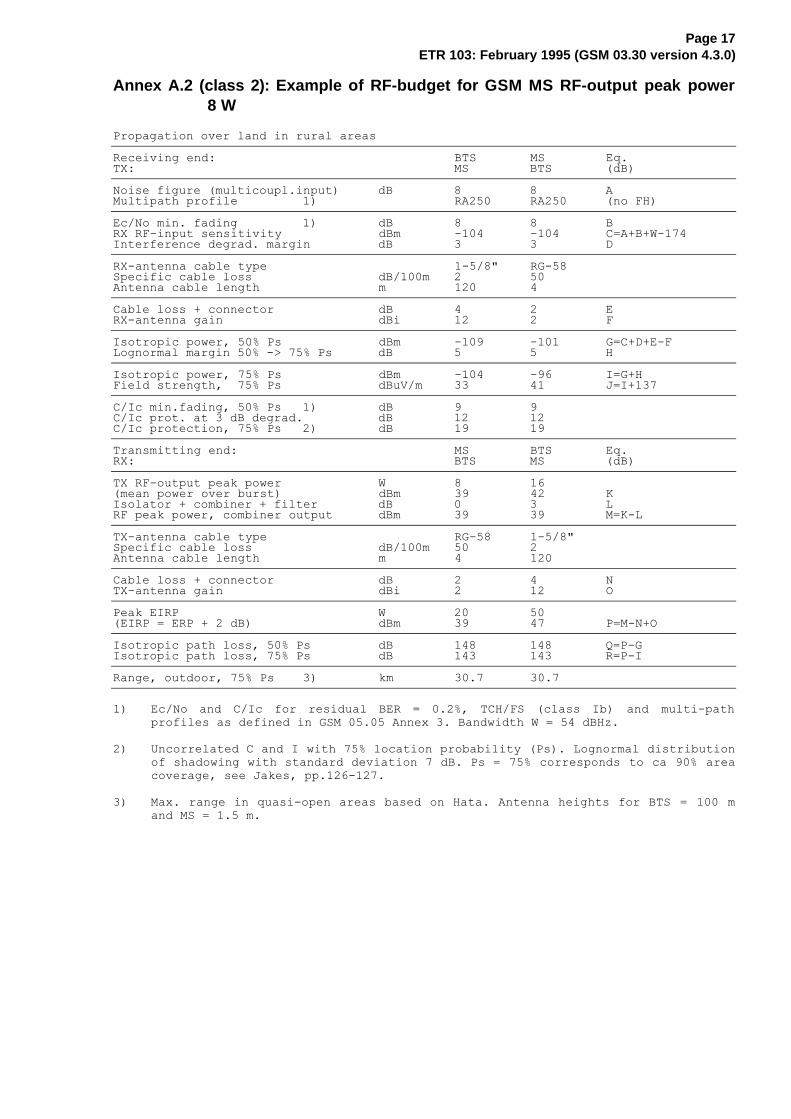
Annex A.2 (class 2): Example of RF-budget for GSM MS RF-output peak power8 W

Propagation over land in rural areas


Noise figure (multicoupl.input) dB 8 8 AMultipath profile 1) RA250 RA250 (no FH)

Ec/No min. fading 1) dB 8 8 BRX RF-input sensitivity dBm -104 -104 C=A+B+W-174Interference degrad. margin dB 3 3 D

RX-antenna cable type 1-5/8" RG-58Specific cable loss dB/100m 2 50Antenna cable length m 120 4

Cable loss + connector dB 4 2 ERX-antenna gain dBi 12 2 F

Isotropic power, 50% Ps dBm -109 -101 G=C+D+E-FLognormal margin 50% -> 75% Ps dB 5 5 H

Isotropic power, 75% Ps dBm -104 -96 I=G+HField strength, 75% Ps dBuV/m 33 41 J=I+137

C/Ic min.fading, 50% Ps 1) dB 9 9C/Ic prot. at 3 dB degrad. dB 12 12C/Ic protection, 75% Ps 2) dB 19 19


TX RF-output peak power W 8 16(mean power over burst) dBm 39 42 KIsolator + combiner + filter dB 0 3 LRF peak power, combiner output dBm 39 39 M=K-L

TX-antenna cable type RG-58 1-5/8"Specific cable loss dB/100m 50 2Antenna cable length m 4 120

Cable loss + connector dB 2 4 NTX-antenna gain dBi 2 12 O

Peak EIRP W 20 50(EIRP = ERP + 2 dB) dBm 39 47 P=M-N+O

Isotropic path loss, 50% Ps dB 148 148 Q=P-GIsotropic path loss, 75% Ps dB 143 143 R=P-I

Range, outdoor, 75% Ps 3) km 30.7 30.7

1) Ec/No and C/Ic for residual BER = 0.2%, TCH/FS (class Ib) and multi-path

profiles as defined in GSM 05.05 Annex 3. Bandwidth W = 54 dBHz.

2) Uncorrelated C and I with 75% location probability (Ps). Lognormal distribution

of shadowing with standard deviation 7 dB. Ps = 75% corresponds to ca 90% area

coverage, see Jakes, pp.126-127.

3) Max. range in quasi-open areas based on Hata. Antenna heights for BTS = 100 m

and MS = 1.5 m.


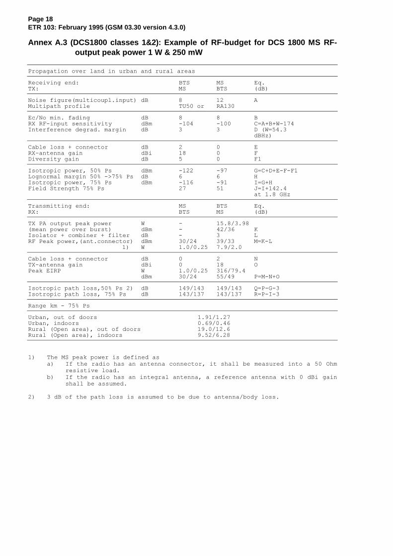
Annex A.3 (DCS1800 classes 1&2): Example of RF-budget for DCS 1800 MS RF-output peak power 1 W & 250 mW

Propagation over land in urban and rural areas


Noise figure(multicoupl.input) dB 8 12 AMultipath profile TU50 or RA130

Ec/No min. fading dB 8 8 BRX RF-input sensitivity dBm -104 -100 C=A+B+W-174Interference degrad. margin dB 3 3 D (W=54.3

dBHz)

Cable loss + connector dB 2 0 ERX-antenna gain dBi 18 0 FDiversity gain dB 5 0 F1

Isotropic power, 50% Ps dBm -122 -97 G=C+D+E-F-F1Lognormal margin 50% ->75% Ps dB 6 6 HIsotropic power, 75% Ps dBm -116 -91 I=G+HField Strength 75% Ps 27 51 J=I+142.4

at 1.8 GHz


TX PA output peak power W - 15.8/3.98(mean power over burst) dBm - 42/36 KIsolator + combiner + filter dB - 3 LRF Peak power,(ant.connector) dBm 30/24 39/33 M=K-L

1) W 1.0/0.25 7.9/2.0

Cable loss + connector dB 0 2 NTX-antenna gain dBi 0 18 OPeak EIRP W 1.0/0.25 316/79.4

dBm 30/24 55/49 P=M-N+O

Isotropic path loss,50% Ps 2) dB 149/143 149/143 Q=P-G-3Isotropic path loss, 75% Ps dB 143/137 143/137 R=P-I-3

Range km - 75% Ps

Urban, out of doors 1.91/1.27Urban, indoors 0.69/0.46Rural (Open area), out of doors 19.0/12.6Rural (Open area), indoors 9.52/6.28

1) The MS peak power is defined as

a) If the radio has an antenna connector, it shall be measured into a 50 Ohm

resistive load.

b) If the radio has an integral antenna, a reference antenna with 0 dBi gain

shall be assumed.

2) 3 dB of the path loss is assumed to be due to antenna/body loss.


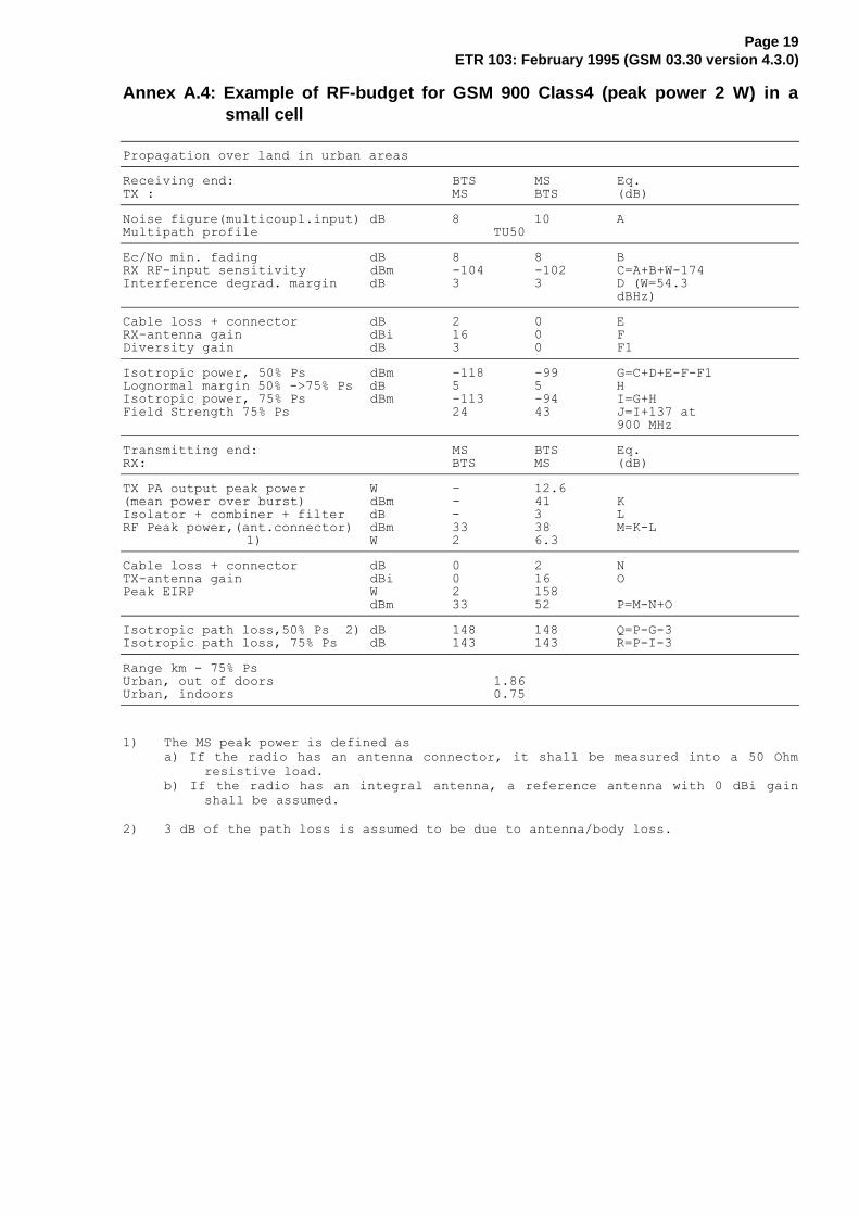
Annex A.4: Example of RF-budget for GSM 900 Class4 (peak power 2 W) in asmall cell

Propagation over land in urban areas

Receiving end: BTS MS Eq.TX : MS BTS (dB)

Noise figure(multicoupl.input) dB 8 10 AMultipath profile TU50

Ec/No min. fading dB 8 8 BRX RF-input sensitivity dBm -104 -102 C=A+B+W-174Interference degrad. margin dB 3 3 D (W=54.3

dBHz)

Cable loss + connector dB 2 0 ERX-antenna gain dBi 16 0 FDiversity gain dB 3 0 F1

Isotropic power, 50% Ps dBm -118 -99 G=C+D+E-F-F1Lognormal margin 50% ->75% Ps dB 5 5 HIsotropic power, 75% Ps dBm -113 -94 I=G+HField Strength 75% Ps 24 43 J=I+137 at

900 MHz


TX PA output peak power W - 12.6(mean power over burst) dBm - 41 KIsolator + combiner + filter dB - 3 LRF Peak power,(ant.connector) dBm 33 38 M=K-L

1) W 2 6.3

Cable loss + connector dB 0 2 NTX-antenna gain dBi 0 16 OPeak EIRP W 2 158

dBm 33 52 P=M-N+O

Isotropic path loss,50% Ps 2) dB 148 148 Q=P-G-3Isotropic path loss, 75% Ps dB 143 143 R=P-I-3

Range km - 75% PsUrban, out of doors 1.86Urban, indoors 0.75

1) The MS peak power is defined as

a) If the radio has an antenna connector, it shall be measured into a 50 Ohm

resistive load.

b) If the radio has an integral antenna, a reference antenna with 0 dBi gain

shall be assumed.

2) 3 dB of the path loss is assumed to be due to antenna/body loss.


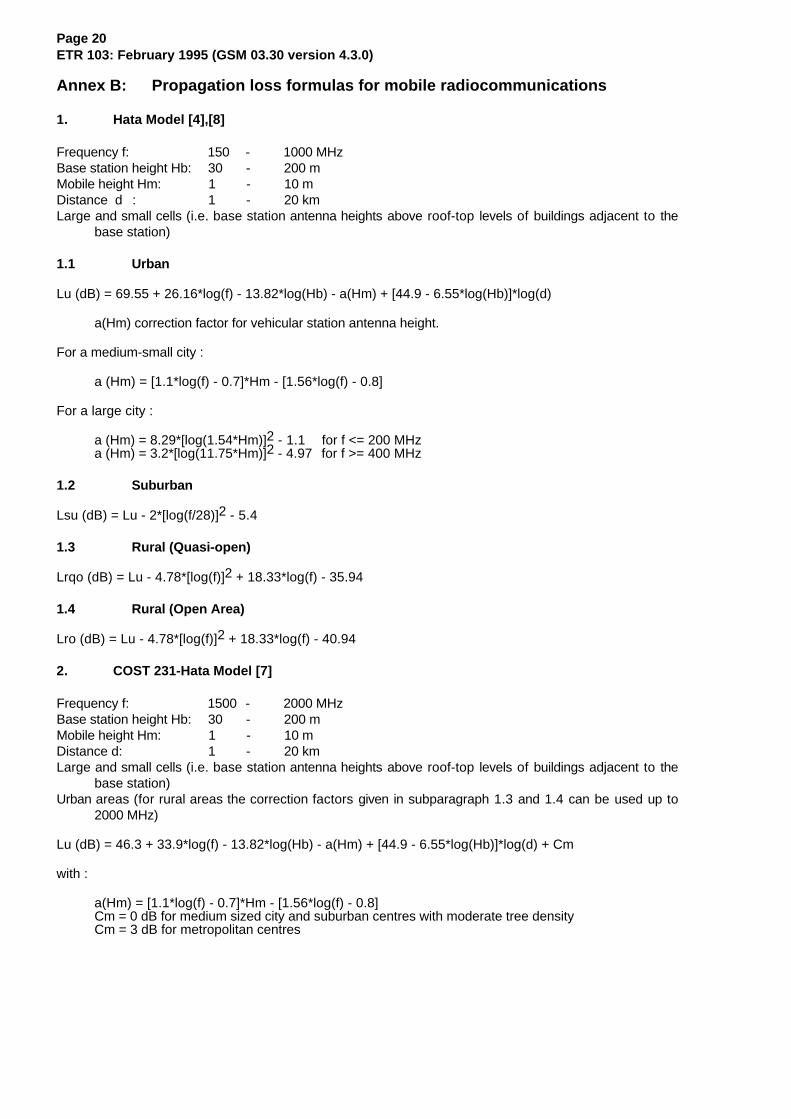
Annex B: Propagation loss formulas for mobile radiocommunications

1. Hata Model [4],[8]

Frequency f: 150 - 1000 MHzBase station height Hb: 30 - 200 mMobile height Hm: 1 - 10 mDistance d : 1 - 20 kmLarge and small cells (i.e. base station antenna heights above roof-top levels of buildings adjacent to the

base station)

1.1 Urban

Lu (dB) = 69.55 + 26.16*log(f) - 13.82*log(Hb) - a(Hm) + [44.9 - 6.55*log(Hb)]*log(d)

a(Hm) correction factor for vehicular station antenna height.

For a medium-small city :

a (Hm) = [1.1*log(f) - 0.7]*Hm - [1.56*log(f) - 0.8]

For a large city :

a (Hm) = 8.29*[log(1.54*Hm)]2 - 1.1 for f <= 200 MHza (Hm) = 3.2*[log(11.75*Hm)]2 - 4.97 for f >= 400 MHz

1.2 Suburban

Lsu (dB) = Lu - 2*[log(f/28)]2 - 5.4

1.3 Rural (Quasi-open)

Lrqo (dB) = Lu - 4.78*[log(f)]2 + 18.33*log(f) - 35.94

1.4 Rural (Open Area)

Lro (dB) = Lu - 4.78*[log(f)]2 + 18.33*log(f) - 40.94

2. COST 231-Hata Model [7]

Frequency f: 1500 - 2000 MHzBase station height Hb: 30 - 200 mMobile height Hm: 1 - 10 mDistance d: 1 - 20 kmLarge and small cells (i.e. base station antenna heights above roof-top levels of buildings adjacent to the

base station)Urban areas (for rural areas the correction factors given in subparagraph 1.3 and 1.4 can be used up to

2000 MHz)

Lu (dB) = 46.3 + 33.9*log(f) - 13.82*log(Hb) - a(Hm) + [44.9 - 6.55*log(Hb)]*log(d) + Cm

with :

a(Hm) = [1.1*log(f) - 0.7]*Hm - [1.56*log(f) - 0.8]Cm = 0 dB for medium sized city and suburban centres with moderate tree densityCm = 3 dB for metropolitan centres


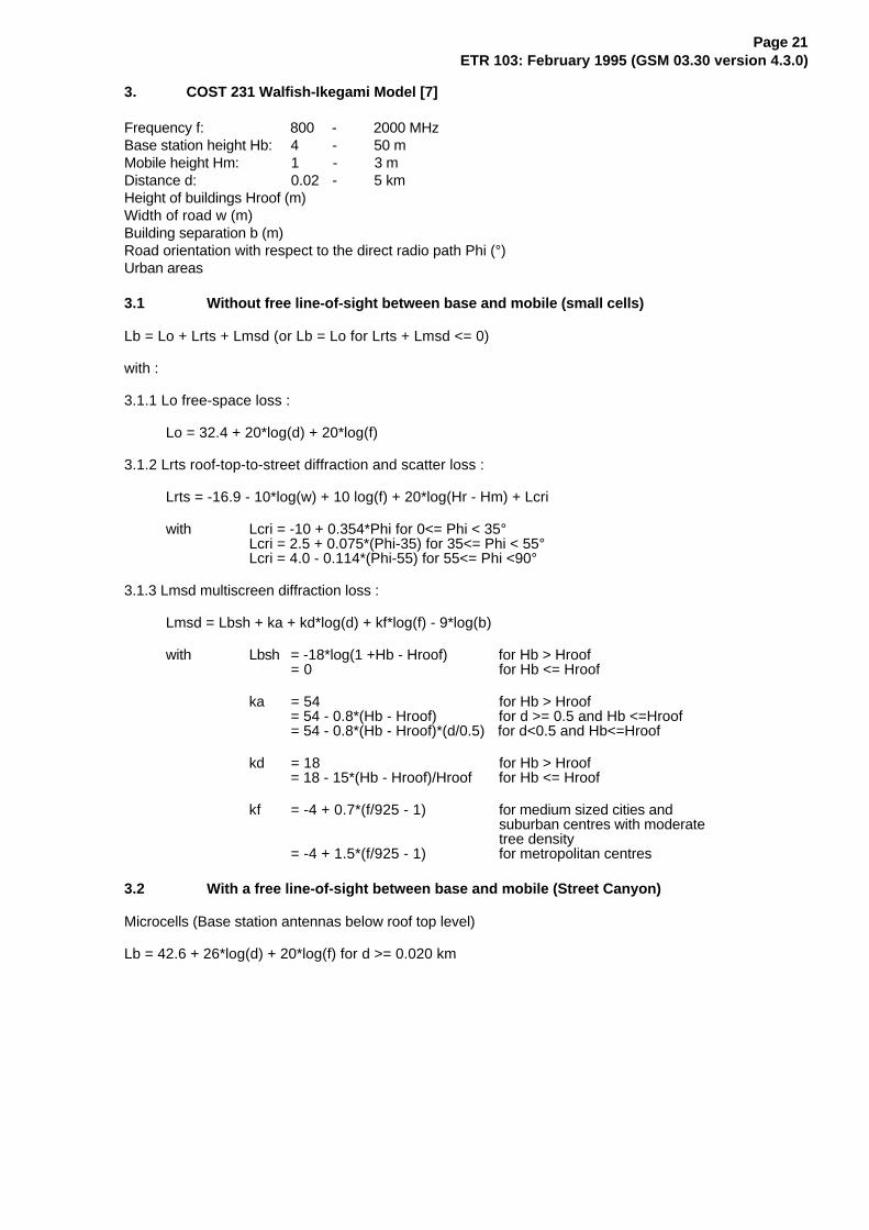
3. COST 231 Walfish-Ikegami Model [7]

Frequency f: 800 - 2000 MHzBase station height Hb: 4 - 50 mMobile height Hm: 1 - 3 mDistance d: 0.02 - 5 kmHeight of buildings Hroof (m)Width of road w (m)Building separation b (m)Road orientation with respect to the direct radio path Phi (°)Urban areas

3.1 Without free line-of-sight between base and mobile (small cells)

Lb = Lo + Lrts + Lmsd (or Lb = Lo for Lrts + Lmsd <= 0)

with :

3.1.1 Lo free-space loss :

Lo = 32.4 + 20*log(d) + 20*log(f)

3.1.2 Lrts roof-top-to-street diffraction and scatter loss :

Lrts = -16.9 - 10*log(w) + 10 log(f) + 20*log(Hr - Hm) + Lcri

with Lcri = -10 + 0.354*Phi for 0<= Phi < 35°Lcri = 2.5 + 0.075*(Phi-35) for 35<= Phi < 55°Lcri = 4.0 - 0.114*(Phi-55) for 55<= Phi <90°

3.1.3 Lmsd multiscreen diffraction loss :

Lmsd = Lbsh + ka + kd*log(d) + kf*log(f) - 9*log(b)

with Lbsh = -18*log(1 +Hb - Hroof) for Hb > Hroof= 0 for Hb <= Hroof

ka = 54 for Hb > Hroof= 54 - 0.8*(Hb - Hroof) for d >= 0.5 and Hb <=Hroof= 54 - 0.8*(Hb - Hroof)*(d/0.5) for d<0.5 and Hb<=Hroof

kd = 18 for Hb > Hroof= 18 - 15*(Hb - Hroof)/Hroof for Hb <= Hroof

kf = -4 + 0.7*(f/925 - 1) for medium sized cities andsuburban centres with moderatetree density

= -4 + 1.5*(f/925 - 1) for metropolitan centres

3.2 With a free line-of-sight between base and mobile (Street Canyon)

Microcells (Base station antennas below roof top level)

Lb = 42.6 + 26*log(d) + 20*log(f) for d >= 0.020 km


Annex C: Path Loss vs Cell Radius

Fig 1. Path loss vs Cell Radius, BS height = 50 m, MS height = 1.5 m (GSM 900).

90

100

110

120

130

140

150

160

170

180

190

200

210

220

1 10 100

Cell radius (km)

path

loss

(dB

)

Urban

Urban Indoor

Suburban

Rural (quasi open)

Rural (open)


Fig 2. Path loss vs Cell Radius, BS height = 100 m, MS height = 1.5 m (GSM 900).

90

100

110

120

130

140

150

160

170

180

190

200

210

220

1 10 100

Cell radius (km)

Pat

h lo

ss (

dB)

Urb an

Urb an ind oor

Sub urba n

Rura l (qua si op en)

Rura l (open)


Fig. 3. Path loss vs Cell Radius, Urban BS height = 50 m, Rural BS height = 60 m, MS height = 1.5 m (DCS 1800)

90

100

110

120

130

140

150

160

170

180

190

200

210

220

1 10 100

Cell Radius ( km)

Pat

h Lo

ss (

dB)

Urb an

Urb an ind oor

Rura l indoor (q uasi open)

Rura l (qua si op en)

Rura l (open)


Fig. 4. Path loss vs Cell Radius for small cells (see section 3.4.2)

0.1 0.5 1.0 3.0100.0

110.0

120.0

130.0

140.0

150.0

160.0

170.0

Path

loss

dB

GSM 900

DCS 1800 (medium sized citiesand suburban centres)

DCS 1800 (metropolitan centres)

Cell Radius (km)

Page 26ETR 103: October 1993 (GSM 03.30 version 4.2.0)

History

Document history

October 1995 First Edition

April 1996 Converted into Adobe Acrobat Portable Document Format (PDF)

Documents

ETR 103 - European digital cellular telecommunication system