A&A 638, A141 (2020)https://doi.org/10.1051/0004-6361/201936865c© S. Pires et al. 2020

Astronomy&Astrophysics

Euclid: Reconstruction of weak-lensing mass mapsfor non-Gaussianity studies?

S. Pires1, V. Vandenbussche1, V. Kansal1, R. Bender2,3, L. Blot4, D. Bonino5, A. Boucaud6, J. Brinchmann7,V. Capobianco5, J. Carretero8, M. Castellano9, S. Cavuoti10,11,12, R. Clédassou13, G. Congedo14, L. Conversi15,L. Corcione5, F. Dubath16, P. Fosalba17,18, M. Frailis19, E. Franceschi20, M. Fumana21, F. Grupp3, F. Hormuth22,

S. Kermiche23, M. Knabenhans24, R. Kohley15, B. Kubik25, M. Kunz26, S. Ligori5, P. B. Lilje27, I. Lloro17,18,E. Maiorano20, O. Marggraf28, R. Massey29, G. Meylan30, C. Padilla8, S. Paltani16, F. Pasian19, M. Poncet13,

D. Potter24, F. Raison3, J. Rhodes31, M. Roncarelli20,32, R. Saglia2,3, P. Schneider28, A. Secroun23, S. Serrano17,33,J. Stadel24, P. Tallada Crespí34, I. Tereno35,36, R. Toledo-Moreo37, and Y. Wang38

(Affiliations can be found after the references)

Received 7 October 2019 / Accepted 6 May 2020

ABSTRACT

Weak lensing, which is the deflection of light by matter along the line of sight, has proven to be an efficient method for constraining models ofstructure formation and reveal the nature of dark energy. So far, most weak-lensing studies have focused on the shear field that can be measureddirectly from the ellipticity of background galaxies. However, within the context of forthcoming full-sky weak-lensing surveys such as Euclid,convergence maps (mass maps) offer an important advantage over shear fields in terms of cosmological exploitation. While it carry the sameinformation, the lensing signal is more compressed in the convergence maps than in the shear field. This simplifies otherwise computationallyexpensive analyses, for instance, non-Gaussianity studies. However, the inversion of the non-local shear field requires accurate control of systematiceffects caused by holes in the data field, field borders, shape noise, and the fact that the shear is not a direct observable (reduced shear). We presentthe two mass-inversion methods that are included in the official Euclid data-processing pipeline: the standard Kaiser & Squires method (KS), and anew mass-inversion method (KS+) that aims to reduce the information loss during the mass inversion. This new method is based on the KS methodand includes corrections for mass-mapping systematic effects. The results of the KS+ method are compared to the original implementation of theKS method in its simplest form, using the Euclid Flagship mock galaxy catalogue. In particular, we estimate the quality of the reconstructionby comparing the two-point correlation functions and third- and fourth-order moments obtained from shear and convergence maps, and weanalyse each systematic effect independently and simultaneously. We show that the KS+ method substantially reduces the errors on the two-pointcorrelation function and moments compared to the KS method. In particular, we show that the errors introduced by the mass inversion on thetwo-point correlation of the convergence maps are reduced by a factor of about 5, while the errors on the third- and fourth-order moments arereduced by factors of about 2 and 10, respectively.

Key words. gravitational lensing: weak – methods: data analysis – dark matter

1. Introduction

Gravitational lensing is the process in which light frombackground galaxies is deflected as it travels towards us. Thedeflection is a result of the gravitation of the intervening mass.Measuring the deformations in a large sample of galaxies offersa direct probe of the matter distribution in the Universe (includ-ing dark matter) and can thus be directly compared to theoreticalmodels of structure formation. The statistical properties of theweak-lensing field can be assessed by a statistical analysis ofeither the shear field or the convergence field. On the one hand,convergence is a direct tracer of the total matter distribution inte-grated along the line of sight, and is therefore directly linkedwith the theory. On the other hand, the shear (or more exactly,the reduced shear) is a direct observable and usually preferredfor simplicity reasons.

Accordingly, the most common method for characterisingthe weak-lensing field distribution is the shear two-point corre-lation function. It is followed very closely by the mass-aperturetwo-point correlation functions, which are the result of convolv-

? This paper is published on behalf of the Euclid Consortium.

ing the shear two-point correlation functions by a compensatedfilter (Schneider et al. 2002) that is able to separate the E andB modes of the two-point correlation functions (Crittenden et al.2002). However, gravitational clustering is a non-linear process,and in particular, the mass distribution is highly non-Gaussianat small scales. For this reason, several estimators of the three-point correlation functions have been proposed, either in theshear field (Bernardeau et al. 2002b; Benabed & Scoccimarro2006) or using the mass-aperture filter (Kilbinger & Schneider2005). The three-point correlation functions are the lowest orderstatistics to quantify non-Gaussianity in the weak-lensing fieldand thus provide additional information on structure formationmodels.

The convergence field can also be used to measure thetwo- and three-point correlation functions and other higher-orderstatistics. When we assume that the mass inversion (the compu-tation of the convergence map from the measured shear field)is properly conducted, the shear field contains the same infor-mation as the convergence maps (e.g. Schneider et al. 2002;Shi et al. 2011). While it carries the same information, thelensing signal is more compressed in the convergence mapsthan in the shear field, which makes it easier to extract and

Open Access article, published by EDP Sciences, under the terms of the Creative Commons Attribution License (https://creativecommons.org/licenses/by/4.0),which permits unrestricted use, distribution, and reproduction in any medium, provided the original work is properly cited.

A141, page 1 of 16

A&A 638, A141 (2020)

computationally less expensive. The convergence maps becomesa new tool that might bring additional constraints complemen-tary to those that we can obtain from the shear field. How-ever, the weak-lensing signal being highly non-Gaussian at smallscales, mass-inversion methods using smoothing or de-noising toregularise the problem are not optimal.

Reconstructing convergence maps from weak lensing is adifficult task because of shape noise, irregular sampling, com-plex survey geometry, and the fact that the shear is not a directobservable. This is an ill-posed inverse problem and requires reg-ularisation to avoid pollution from spurious B modes. Severalmethods have been derived to reconstruct the projected mass dis-tribution from the observed shear field. The first non-parametricmass reconstruction was proposed by Kaiser & Squires (1993)and was further improved by Bartelmann (1995), Kaiser (1995),Schneider (1995), and Squires & Kaiser (1996). These linearinversion methods are based on smoothing with a fixed ker-nel, which acts as a regularisation of the inverse problem. Non-linear reconstruction methods were also proposed using differentsets of priors and noise-regularisation techniques (Bridle et al.1998; Seitz et al. 1998; Marshall et al. 2002; Pires et al. 2009a;Jullo et al. 2014; Lanusse et al. 2016). Convergence mass mapshave been built from many surveys, including the COSMOSSurvey (Massey et al. 2007), the Canada France Hawaï Tele-scope Lensing Survey CFHTLenS (Van Waerbeke et al. 2013),the CFHT/MegaCam Stripe-82 Survey (Shan et al. 2014), theDark Energy Survey Science Verification DES SV (Chang et al.2015; Vikram et al. 2015; Jeffrey et al. 2018), the Red ClusterSequence Lensing Survey RCSLenS (Hildebrandt et al. 2016),and the Hyper SuprimeCam Survey (Oguri et al. 2018). With theexception of Jeffrey et al. (2018), who used the non-linear recon-struction proposed by Lanusse et al. (2016), all these methodsare based on the standard Kaiser & Squires method.

In the near future, several wide and deep weak-lensing sur-veys are planned: Euclid (Laureijs et al. 2011), Large Synop-tic Survey Telescope LSST (LSST Science Collaboration et al.2009), and Wide Field Infrared Survey Telescope WFIRST(Green et al. 2012). In particular, the Euclid satellite will sur-vey 15 000 deg2 of the sky to map the geometry of the darkUniverse. One of the goals of the Euclid mission is to pro-duce convergence maps for non-Gaussianity studies and con-strain cosmological parameters. To do this, two different massinversion methods are being included into the official Euclid dataprocessing pipeline. The first method is the standard Kaiser &Squires method (hereafter KS). Although it is well known thatthe KS method has several shortcomings, it is taken as the refer-ence for cross-checking the results. The second method is a newnon-linear mass-inversion method (hereafter KS+) based on theformalism developed in Pires et al. (2009a). The KS+ methodaims at performing the mass inversion with minimum informa-tion loss. This is done by performing the mass inversion withno other regularisation than binning while controlling systematiceffects.

In this paper, the performance of these two mass-inversionmethods is investigated using the Euclid Flagship mock galaxycatalogue (version 1.3.3, Castander et al., in prep.) with real-istic observational effects (i.e. shape noise, missing data, andthe reduced shear). The effect of intrinsic alignments is notstudied in this paper because we lack simulations that wouldproperly model intrinsic alignments. However, intrinsic align-ments also need to be considered seriously because theyaffect second- and higher-order statistics. A contribution ofseveral percent is expected to two-point statistics (see e.g.Joachimi et al. 2013).

We compare the results obtained with the KS+ method tothose obtained with a version of the KS method in which nosmoothing step is performed other than binning. We quantify thequality of the reconstruction using two-point correlation func-tions and moments of the convergence. Our tests illustrate theefficacy of the different mass-inversion methods in preservingthe second-order statistics and higher-order moments.

The paper is organised as follows. In Sect. 2 we presentthe weak-lensing mass-inversion problem and the standard KSmethod. Section 2.2 presents the KS+ method we used to cor-rect for the different systematic effects. In Sect. 4 we explainthe method with which we compared these two mass-inversionmethods. In Sect. 5 we use the Euclid Flagship mock galaxy cat-alogue with realistic observational effects such as shape noiseand complex survey geometry and consider the reduced shear toinvestigate the performance of the two mass-inversion methods.First, we derive simulations including only one issue at a time totest each systematic effect independently. Then we derive real-istic simulations that include them all and study the systematiceffects simultaneously. We conclude in Sect. 6.

2. Weak-lensing mass inversion

2.1. Weak gravitational lensing formalism

In weak-lensing surveys, the shear field γ(θ) is derived from theellipticities of the background galaxies at position θ in the image.The two components of the shear can be written in terms ofthe lensing potential ψ(θ) as (see e.g. Bartelmann & Schneider2001)

γ1 = 12

(∂2

1 − ∂22

)ψ,

γ2 = ∂1∂2ψ,(1)

where the partial derivatives ∂i are with respect to the angularcoordinates θi, i = 1, 2 representing the two dimensions of skycoordinates. The convergence κ(θ) can also be expressed in termsof the lensing potential as

κ =12

(∂2

1 + ∂22

)ψ. (2)

For large-scale structure lensing, assuming a spatially flat Uni-verse, the convergence at a sky position θ from sources at comov-ing distance r is defined by

κ(θ, r) =3H2

0Ωm

2c2

∫ r

0dr′

r′(r − r′)r

δ(θ, r′)a(r′)

, (3)

where H0 is the Hubble constant, Ωm is the matter density, a isthe scale factor, and δ ≡ (ρ− ρ)/ρ is the density contrast (where ρand ρ are the 3D density and the mean 3D density, respectively).In practice, the expression for κ can be generalised to sourceswith a distribution in redshift, or equivalently, in comoving dis-tance f (r), yielding

κ(θ) =3H2

0Ωm

2c2

∫ rH

0dr′p(r′)r′

δ(θ, r′)a(r′)

, (4)

where rH is the comoving distance to the horizon. The con-vergence map reconstructed over a region on the sky gives usthe integrated mass-density fluctuation weighted by the lensing-weight function p(r′),

p(r′) =

∫ rH

r′dr f (r)

r − r′

r· (5)

A141, page 2 of 16

S. Pires et al.: Euclid: Reconstruction of weak-lensing mass maps for non-Gaussianity studies

2.2. Kaiser & Squires method (KS)

2.2.1. KS mass-inversion problem

The weak lensing mass inversion problem consists of recon-structing the convergence κ from the measured shear field γ.We can use complex notation to represent the shear field, γ =γ1 + iγ2, and the convergence field, κ = κE + iκB, with κE corre-sponding to the curl-free component and κB to the gradient-freecomponent of the field, called E and B modes by analogy withthe electromagnetic field. Then, from Eq. (1) and Eq. (2), we canderive the relation between the shear field γ and the convergencefield κ. For this purpose, we take the Fourier transform of theseequations and obtain

γ = P κ, (6)

where the hat symbol denotes Fourier transforms, P = P1 + iP2,

P1(`) =`2

1−`22

`2 ,

P2(`) = 2`1`2`2 ,

(7)

with `2 ≡ `21 + `2

2 and `i the wave numbers corresponding to theangular coordinates θi.

P is a unitary operator. The inverse operator is its complexconjuguate P∗ = P1−iP2 , as shown by Kaiser & Squires (1993),

κ = P∗ γ. (8)

We note that to recover κ from γ, there is a degeneracy when`1 = `2 = 0. Therefore the mean value of κ cannot be recov-ered if only shear information is available. This is the so-calledmass-sheet degeneracy (see e.g. Bartelmann 1995, for a discus-sion). In practice, we impose that the mean convergence vanishesacross the survey by setting the reconstructed ` = 0 mode tozero. This is a reasonable assumption for large-field reconstruc-tion (e.g. Seljak 1998).

We can easily derive an estimator of the E-mode and B-modeconvergence in the Fourier domain,

ˆκE = P1γ1 + P2γ2,

ˆκB = −P2γ1 + P1γ2.(9)

Because the weak lensing arises from a scalar potential (the lens-ing potential ψ), it can be shown that weak lensing only producesE modes. However, intrinsic alignments and imperfect correc-tions of the point spread function (PSF) generally generate bothE and B modes. The presence of B modes can thus be used to testfor residual systematic effects in current weak-lensing surveys.

2.2.2. Missing-data problem in weak lensing

The shear is only sampled at the discrete positions of the galaxieswhere the ellipticity is measured. The first step of the mass map-inversion method therefore is to bin the observed ellipticities ofgalaxies on a regular pixel grid to create what we refer to as theobserved shear maps γobs. Some regions remain empty becausevarious masks were applied to the data, such as the masking-outof bright stars or camera CCD defects. In such cases, the shearis set to zero in the original KS method,

γobs = Mγn, (10)

with M the binary mask (i.e. M = 1 when we have informationat the pixel, M = 0 otherwise) and γn the noisy shear maps. As

the shear at any sky position is non-zero in general, this intro-duces errors in the reconstructed convergence maps. Some spe-cific methods address this problem by discarding masked pixelsat the noise-regularisation step (e.g. Van Waerbeke et al. 2013).However, as explained previously, this intrinsic filtering resultsin subtantial signal loss at small scales. Instead, inpainting tech-niques are used in the KS+ method to fill the masked regions(see Appendix A).

2.2.3. Weak-lensing shape noise

The gravitational shear is derived from the ellipticities of thebackground galaxies. However, the galaxies are not intrinsicallycircular, therefore their measured ellipticity is a combination oftheir intrinsic ellipticity and the gravitational lensing shear. Theshear is also subject to measurement noise and uncertainties inthe PSF correction. All these effects can be modelled as an addi-tive noise, N = N1 + iN2,

γn = γ + N (11)

The noise terms N1 and N2 are assumed to be Gaussian anduncorrelated with zero mean and standard deviation,

σin =

σε√N i

g

, (12)

where N ig is the number of galaxies in pixel i. The root-mean-

square shear dispersion per galaxy, σε , arises both from themeasurement uncertainties and the intrinsic shape dispersionof galaxies. The Gaussian assumption is a reasonable assump-tion, and σε is set to 0.3 for each component as is gener-ally found in weak-lensing surveys (e.g. Leauthaud et al. 2007;Schrabback et al. 2015, 2018). The surface density of usablegalaxies is expected to be around ng = 30 gal. arcmin−2 for theEuclid Wide survey (Cropper et al. 2013).

The derived convergence map is also subject to an additivenoise,

ˆκn = P∗ γn = κ + P∗ N. (13)

In particular, the E component of the convergence noise is

NE = N1 ∗ P1 + N2 ∗ P2, (14)

where the asterisk denotes the convolution operator, and P1 andP2 are the inverse Fourier transforms of P1 and P2. When theshear noise terms N1 and N2 are Gaussian, uncorrelated, andwith a constant standard deviation across the field, the conver-gence noise is also Gaussian and uncorrelated. In practice, thenumber of galaxies varies slightly across the field. The variancesof N1 and N2 might also be slightly different, which can be mod-elled by different values of σε for each component. These effectsintroduce noise correlations in the convergence noise maps, butthey were found to remain negligible compared to other effectsstudied in this paper.

In the KS method, a smoothing by a Gaussian filter is fre-quently applied to the background ellipticities before mass inver-sion to regularise the solution. Although performed in mostapplications of the KS method, this noise regularisation stepis not mandatory. It was introduced to avoid infinite noiseand divergence at very small scales. However, the pixelisationalready provides an intrinsic regularisation. This means thatthere is no need for an additional noise regularisation prior tothe inversion. Nonetheless, for specific applications that requiredenoising in any case, the filtering step can be performed beforeor after the mass inversion.

A141, page 3 of 16

A&A 638, A141 (2020)

3. Improved Kaiser & Squires method (KS+)

Systematic effects in mass-inversion techniques must be fullycontrolled in order to use convergence maps as cosmologicalprobes for future wide-field weak-lensing experiments such asEuclid. We introduce the KS+ method based on the formalismdeveloped in Pires et al. (2009a) and Jullo et al. (2014), whichintegrates the necessary corrections for imperfect and realisticmeasurements. We summarise its improvements over KS in thissection and evaluate its performance in Sect. 5.

In this paper, the mass-mapping formalism is developed inthe plane. The mass inversion can also be performed on thesphere, as proposed in Pichon et al. (2010) and Chang et al.(2018), and the extension of the KS+ method to the curved sky isbeing investigated. However, the computation time and memoryrequired to process the spherical mass inversion means limita-tions in terms of convergence maps resolution and/or complexityof the algorithm. Thus, planar mass inversions remain importantfor reconstructing convergence maps with a good resolution andprobing the non-Gaussian features of the weak-lensing field (e.g.for peak-count studies).

3.1. Missing data

When the weak-lensing shear field γ is sampled on a grid ofN×N pixels, we can describe the complex shear and convergencefields by their respective matrices. In the remaining paper, thenotations γ and κ stand for the matrix quantities.

In the standard version of the KS method, the pixels with nogalaxies are set to zero. Figure 1 shows an example of simulatedshear maps without shape noise derived from the Euclid Flag-ship mock galaxy catalogue (see Sect. 4.3 for more details). Theupper panels of Fig. 1 show the two components of the shear withzero values (displayed in black) corresponding to the mask of themissing data. These zero values generate an important leakageduring the mass inversion.

With KS+, the problem is reformulated by including addi-tional assumptions to regularise the problem. The convergenceκ can be analysed using a transformation Φ, which yields a setof coefficients α = ΦTκ (Φ is an orthogonal matrix operator,and ΦT represents the transpose matrix of Φ). In the case ofthe Fourier transformation, ΦT would correspond to the discreteFourier transform (DFT) matrix, and α would be the Fouriercoefficients of κ. The KS+ method uses a prior of sparsity, thatis, it assumes that there is a transformation Φ where the conver-gence κ can be decomposed into a set of coefficients α, wheremost of its coefficients are close to zero. In this paper, Φ waschosen to be the discrete cosine transform (DCT) followingPires et al. (2009a). The DCT expresses a signal in terms of asum of cosine functions with different frequencies and ampli-tudes. It is similar to the DFT, but uses smoother boundary con-ditions. This provides a sparser representation. Hence the use ofthe DCT for JPEG compression.

We can rewrite the relation between the observed shear γobs

and the noisy convergence κn as

γobs = MPκn, (15)

with M being the mask operator and P the KS mass-inversionoperator. There is an infinite number of convergence κn thatcan fit the observed shear γobs. With KS+, we first impose thatthe mean convergence vanishes across the survey, as in the KSmethod. Then, among all possible solutions, KS+ searches forthe sparsest solution κn in the DCT Φ (i.e. the convergence κn

that can be represented with the fewest large coefficients). The

solution of this mass-inversion problem is obtained by solving

minκn‖ΦTκn‖0 subject to ‖ γobs −MPκn ‖2≤ σ2, (16)

where ||z||0 the pseudo-norm, that is, the number of non-zeroentries in z, ||z|| the classical l2 norm (i.e. ||z|| =

√∑k(zk)2), and

σ stands for the standard deviation of the input shear map mea-sured outside the mask. The solution of this optimisation task canbe obtained through an iterative thresholding algorithm calledmorphological component analysis (MCA), which was intro-duced by Elad et al. (2005) and was adapted to the weak-lensingproblem in Pires et al. (2009a).

Pires et al. (2009a) used an additional constraint to force theB modes to zero. This is optimal when the shear maps haveno B modes. However, any real observation has some resid-ual B modes as a result of intrinsic alignments, imperfect PSFcorrection, etc. The B-mode power is then transferred to the Emodes, which degrades the E-mode convergence reconstruction.We here instead let the B modes free, and an additional con-straint was set on the power spectrum of the convergence map.To this end, we used a wavelet transform to decompose the con-vergence maps into a set of aperture mass maps using the star-let transform algorithm (Starck et al. 1998; Starck & Murtagh2002). Then, the constraint consists of renormalising the stan-dard deviation (or equivalently, the variance) of each aperturemass map inside the mask regions to the values measured in thedata, outside the masks, and then reconstructing the convergencethrough the inverse wavelet transform. The variance per scalecorresponding to the power spectrum at these scales allows usto constrain a broadband power spectrum of the convergence κinside the gaps.

Adding the power spectrum constraints yields the final sparseoptimisation problem,

minκn‖ΦTκn‖0 s.t. ‖ γobs −MPWTQWκn ‖2≤ σ2, (17)

where W is the forward wavelet transform and WT its inversetransform, and Q is the linear operator used to impose the powerspectrum constraint. More details about the KS+ algorithm aregiven in Appendix A.

The KS+ method allows us to reconstruct the in-painted con-vergence maps and the corresponding in-painted shear maps,where the empty pixels are replaced by non-zero values. Theseinterpolated values preserve the continuity of the signal andreduce the signal leakage during the mass inversion (see lowerpanels of Fig. 1). The quality of the convergence maps recon-struction with respect to missing data is evaluated in Sect. 5.Additionally, the new constraint allows us to use the residualB modes of the reconstructed maps to test for the presence ofresidual systematic effects and possibly validate the shear mea-surement processing chain.

3.2. Field border effects

The KS and KS+ mass-inversion methods relate the conver-gence and the shear fields in Fourier space. However, the discreteFourier transform implicitly assumes that the image is periodicalong both dimensions. Because there is no reason for oppo-site borders to be alike, the periodic image generally presentsstrong discontinuities across the frame border. These disconti-nuities cause several artefacts at the borders of the reconstructedconvergence maps. The field border effects can be addressed byremoving the image borders, which throws away a large fractionof the data. Direct finite-field mass-inversion methods have also

A141, page 4 of 16

S. Pires et al.: Euclid: Reconstruction of weak-lensing mass maps for non-Gaussianity studies

0 100 200 300 400 500x [pixels]

0

100

200

300

400

500y [pixels]

−0.10

−0.08

−0.06

−0.04

−0.02

0.00

0.02

0.04

0.06

0.08

0.10

0 100 200 300 400 500x [pixels]

0

100

200

300

400

500

y [pixels]

−0.10

−0.08

−0.06

−0.04

−0.02

0.00

0.02

0.04

0.06

0.08

0.10

0 100 200 300 400 500x [pixels]

0

100

200

300

400

500

y [pixels]

−0.10

−0.08

−0.06

−0.04

−0.02

0.00

0.02

0.04

0.06

0.08

0.10

0 100 200 300 400 500x [pixels]

0

100

200

300

400

500

y [pixels]

−0.10

−0.08

−0.06

−0.04

−0.02

0.00

0.02

0.04

0.06

0.08

0.10

Fig. 1. Simulated shear maps with missing data covering a field of 5 × 5. Left panels: first component of the shear γ1, and right panels: secondcomponent of the shear γ2. Upper panels: incomplete shear maps, where the pixels with no galaxies are set to zero (displayed in black). Lowerpanels: result of the inpainting method that allows us to fill the gaps judiciously.

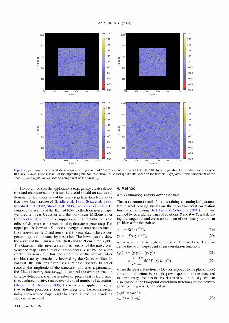
been proposed (e.g. Seitz & Schneider 1996, 2001). Althoughunbiased, convergence maps reconstructed using these methodsare noisier than those obtained with the KS method. In the KS+method, the problem of borders is solved by taking larger sup-port for the image and by considering the borders as maskedregions to be in-painted. The upper panels of Fig. 2 show thetwo components of a shear map covering 5 × 5 degrees andextending to a field of 10 × 10. The inpainting method is thenused to recover the shear at the field boundaries, as shown in thelower panels of Fig. 2. After the mass inversion is performed,the additional borders are removed. This technique reduces thefield border effects by pushing the border discontinuities fartheraway.

3.3. Reduced shear

In Sect. 2.2 we assumed knowledge of the shear, in which casethe mass inversion is linear. In practice, the observed galaxyellipticity is not induced by the shear γ, but by the reduced shearg that depends on the convergence κ corresponding to that par-ticular line of sight,

g ≡γ

1 − κ· (18)

While the difference between the shear γ and the reduced shearg is small in the regime of cosmic shear (κ 1), neglectingit might nevertheless cause a measurable bias at small angular

scales (see e.g. White 2005; Shapiro 2009). In the standard ver-sion of KS, the Fourier estimators are only valid when the con-vergence is small (κ 1), and they no longer hold near thecentre of massive galaxy clusters. The mass-inversion problembecomes non-linear, and it is therefore important to properlyaccount for reduced shear.

In the KS+ method, an iterative scheme is used to recoverthe E-mode convergence map, as proposed in Seitz & Schneider(1995). The method consists of solving the linear inverse prob-lem iteratively (see Eq. (9)), using at each iteration the previousestimate of the E-mode convergence to correct the reduced shearusing Eq. (18). Each iteration then provides a better estimateof the shear. This iterative algorithm was found in Jullo et al.(2014) to quickly converge to the solution (about three itera-tions). The KS+ method uses the same iterative scheme to cor-rect for reduced shear, and we find that it is a reasonable assump-tion in the case of large-scale structure lensing.

3.4. Shape noise

In the original implementation of KS, the shear maps are firstregularised with a smoothing window (i.e. a low-pass filter) toobtain a smoothed version of the shear field. Then, Eq. (9) isapplied to derive the convergence maps. In contrast, the KS+method aims at producing very general convergence maps formany applications. In particular, it produces noisy maps withminimum information loss.

A141, page 5 of 16

A&A 638, A141 (2020)

0 200 400 600 800 1000x [pixels]

0

200

400

600

800

1000y [pixels]

−0.10

−0.08

−0.06

−0.04

−0.02

0.00

0.02

0.04

0.06

0.08

0.10

0 200 400 600 800 1000x [pixels]

0

200

400

600

800

1000

y [pixels]

−0.10

−0.08

−0.06

−0.04

−0.02

0.00

0.02

0.04

0.06

0.08

0.10

0 200 400 600 800 1000x [pixels]

0

200

400

600

800

1000

y [pixels]

−0.10

−0.08

−0.06

−0.04

−0.02

0.00

0.02

0.04

0.06

0.08

0.10

0 200 400 600 800 1000x [pixels]

0

200

400

600

800

1000

y [pixels]

−0.10

−0.08

−0.06

−0.04

−0.02

0.00

0.02

0.04

0.06

0.08

0.10

Fig. 2. Upper panels: simulated shear maps covering a field of 5 × 5, extended to a field of 10 × 10 by zero padding (zero values are displayedin black). Lower panels: result of the inpainting method that allows us to extrapolate the shear on the borders. Left panels: first component of theshear γ1, and right panels: second component of the shear γ2.

However, for specific applications (e.g. galaxy cluster detec-tion and characterisation), it can be useful to add an additionalde-noising step, using any of the many regularisation techniquesthat have been proposed (Bridle et al. 1998; Seitz et al. 1998;Marshall et al. 2002; Starck et al. 2006; Lanusse et al. 2016). Tocompare the results of the KS and KS+ methods on noisy maps,we used a linear Gaussian and the non-linear MRLens filter(Starck et al. 2006) for noise suppression. Figure 3 illustrates theeffect of shape noise on reconstructing the convergence map. Theupper panels show one E-mode convergence map reconstructedfrom noise-free (left) and noisy (right) shear data. The conver-gence map is dominated by the noise. The lower panels showthe results of the Gaussian filter (left) and MRLens filter (right).The Gaussian filter gives a smoothed version of the noisy con-vergence map, whose level of smoothness is set by the widthof the Gaussian (σ). Thus, the amplitude of the over-densities(in blue) are systematically lowered by the Gaussian filter. Incontrast, the MRLens filter uses a prior of sparsity to betterrecover the amplitude of the structures and uses a parameter,the false-discovery rate (αFDR), to control the average fractionof false detections (i.e. the number of pixels that is truly inac-tive, declared positive) made over the total number of detections(Benjamini & Hochberg 1995). For some other applications (e.g.two- or three-point correlation), the integrity of the reconstructednoisy convergence maps might be essential and this denoisingstep can be avoided.

4. Method

4.1. Comparing second-order statistics

The most common tools for constraining cosmological parame-ters in weak-lensing studies are the shear two-point correlationfunctions. Following Bartelmann & Schneider (2001), they aredefined by considering pairs of positions ϑ and θ + ϑ, and defin-ing the tangential and cross-component of the shear γt and γ× atposition ϑ for this pair as

γt = −Re(γ e−2iϕ), (19)

γ× = −Im(γ e−2iϕ), (20)

where ϕ is the polar angle of the separation vector θ. Then wedefine the two independent shear correlation functions

ξ±(θ) : = 〈γtγ′t 〉 ± 〈γ×γ

′×〉 (21)

=1

2π

∫ ∞

0d` ` Pκ(`) J0,4(`θ), (22)

where the Bessel function J0 (J4) corresponds to the plus (minus)correlation function, Pκ(`) is the power spectrum of the projectedmatter density, and ` is the Fourier variable on the sky. We canalso compute the two-point correlation functions of the conver-gence (κ = κE + iκB), defined as

ξκE (θ) = 〈κEκ′E〉,

ξκB (θ) = 〈κBκ′B〉. (23)

A141, page 6 of 16

S. Pires et al.: Euclid: Reconstruction of weak-lensing mass maps for non-Gaussianity studies

0 100 200 300 400 500x [pixels]

0

100

200

300

400

500y [pixels]

−0.05

0.00

0.05

0.10

0.15

0.20

0.25

0.30

0.35

0.40

0 100 200 300 400 500x [pixels]

0

100

200

300

400

500

y [pixels]

−0.40

−0.32

−0.24

−0.16

−0.08

0.00

0.08

0.16

0.24

0.32

0.40

0 100 200 300 400 500x [pixels]

0

100

200

300

400

500

y [pixels]

−0.05

0.00

0.05

0.10

0.15

0.20

0.25

0.30

0.35

0.40

0 100 200 300 400 500x [pixels]

0

100

200

300

400

500

y [pixels]

−0.05

0.00

0.05

0.10

0.15

0.20

0.25

0.30

0.35

0.40

Fig. 3. Shape-noise effect. Upper panels: original E-mode convergence κ map (left) and the noisy convergence map with ng = 30 gal. arcmin−2

(right). Lower panels: reconstructed maps using a linear Gaussian filter with a kernel size of σ = 3′ (left) and the non-linear MRLens filteringusing αFDR = 0.05 (right). The field is 5 × 5 downsampled to 512 × 512 pixels.

We can verify that these two quantities agree (Schneider et al.2002):

ξ+(θ) = ξκE (θ) + ξκB (θ). (24)

When the B modes in the shear field are consistent with zero,the two-point correlation of the shear (ξ+) is equal to the two-point correlation of the convergence (ξκE ). Then the differencesbetween the two are due to the errors introduced by the massinversion to go from shear to convergence.

We computed these two-point correlation functions using thetree code athena (Kilbinger et al. 2014). The shear two-pointcorrelation functions were computed by averaging over pairs ofgalaxies of the mock galaxy catalogue, whereas the convergencetwo-point correlation functions were computed by averagingover pairs of pixels in the convergence map. The convergencetwo-point correlation functions can only be computed for sep-aration vectors θ allowed by the binning of the convergencemap.

4.2. Comparing higher-order statistics

Two-point statistics cannot fully characterise the weak-lensingfield at small scales where it becomes non-Gaussian (e.g.Bernardeau et al. 2002a). Because the small-scale features carryimportant cosmological information, we computed the third-order moment, 〈κ3

E〉, and the fourth-order moment, 〈κ4E〉, of the

convergence. Computations were performed on the original con-vergence maps provided by the Flagship simulation, as well ason the convergence maps reconstructed from the shear field withthe KS and KS+ methods. We evaluated the moments of con-vergence at various scales by computing aperture mass maps(Schneider 1996; Schneider et al. 1998). Aperture mass mapsare typically obtained by convolving the convergence maps witha filter function of a specific scale (i.e. aperture radii). We per-formed this here by means of a wavelet transform using the star-let transform algorithm (Starck et al. 1998; Starck & Murtagh2002), which simultaneously produces a set of aperture massmaps on dyadic (powers of two) scales (see Appendix A formore details). Leonard et al. (2012) demonstrated that the aper-ture mass is formally identical to a wavelet transform at a specificscale and the aperture mass filter corresponding to this transformis derived. The wavelet transform offers significant advantagesover the usual aperture mass algorithm in terms of computationtime, providing speed-up factors of about 5 to 1200 dependingon the scale.

4.3. Numerical simulations

We used the Euclid Flagship mock galaxy catalogue version 1.3.3(Castander et al., in prep.) derived from N-body cosmologicalsimulation (Potter et al. 2017) with parameters Ωm = 0.319,Ωb = 0.049, ΩΛ = 0.681, σ8 = 0.83, ns = 0.96, h = 0.67,and the particle mass was mp ∼ 2.398 × 109 M h−1. The galaxy

A141, page 7 of 16

A&A 638, A141 (2020)

Fig. 4. Missing data effects: Pixel difference outside the mask between the original E-mode convergence κ map and the map reconstructed fromthe incomplete simulated noise-free shear maps using the KS method (le f t) and the KS+ method (right). The field is 10 × 10 downsampled to1024 × 1024 pixels. The missing data represent roughly 20% of the data.

light-cone catalogue contains 2.6 billion galaxies over 5000 deg2,and it extends up to z = 2.3. It has been built using ahybrid halo occupation distribution and halo abundance match-ing (HOD+HAM) technique, whose galaxy-clustering propertieswere discussed in detail in Crocce et al. (2015). The lensing prop-erties were computed using the Born approximation and projectedmass density maps (in HEALPix format with Nside = 8192) gener-ated from the particle light-cone of the Flagship simulation. Moredetails on the lensing properties of the Flagship mock galaxy cat-alogue can be found in Fosalba et al. (2015, 2008).

In order to evaluate the errors introduced by the mass-mapping methods, we extracted ten contiguous shear and con-vergence fields of 10 × 10 from the Flagship mock galaxycatalogue, yielding a total area of 1000 deg2. The fields cor-respond to galaxies that lie in the range of 15 < α < 75and 15 < δ < 35, where α and δ are the right ascension anddeclination, respectively. In order to obtain the density of30 galaxies per arcmin2 foreseen for the Euclid Wide survey, werandomly selected one quarter of all galaxies in the catalogue.Then projected shear and convergence maps were constructed bycombining all the redshifts of the selected galaxies. More sophis-ticated selection methods based on galaxy magnitude would pro-duce slightly different maps. However, they would not changethe performances of the two methods we studied here. The fieldswere down-sampled to 1024 × 1024 pixels, which correspondsto a pixel size of about 0′.6. Throughout all the paper, the shadedregions stand for the uncertainties on the mean estimated fromthe total 1000 deg2 of the ten fields. Because the Euclid Widesurvey is expected to be 15 000 deg2, the sky coverage will be15 times larger than the current mock. Thus, the uncertaintieswill be smaller by a factor of about 4.

4.4. Shear field projection

We considered fields of 10×10. The fields were taken to be suf-ficiently small to be approximated by a tangent plane. We used agnomonic projection to project the points of the celestial sphereonto a tangent plane, following Pires et al. (2012a), who foundthat this preserves the two-point statistics. We note, however,that higher-order statistics may behave differently under differ-ent projections.

The shear field projection is obtained by projecting thegalaxy positions from the sphere (α, δ) in the catalogue onto

a tangent plane (x, y). The projection of a non-zero spin fieldsuch as the shear field requires a projection of both the galaxypositions and their orientations. Projections of the shear do notpreserve the spin orientation, which can generate substantialB modes (depending on the declination) if not corrected for. Twoproblems must be considered because of the orientation. First,the projection of the meridians are not parallel, so that north isnot the same everywhere in the same projected field of view. Sec-ond, the projection of the meridians and great circles is not per-pendicular, so that the system is locally non-Cartesian. Becausewe properly correct for the other effects (e.g. shape noise, miss-ing data, or border effects) and consider large fields of view(10 × 10) possibly at high latitudes, these effects need to beconsidered. The first effect is dominant and generates substantialB modes (increasing with latitude) if not corrected for. This canbe easily corrected for by measuring the shear orientation withrespect to local north. We find that this correction is sufficient forthe residual errors due to projection to become negligible com-pared to errors due to other effects.

5. Systematic effects on the mass-map inversion

In this section, we quantify the effect of field borders, missingdata, shape noise, and the approximation of shear by reducedshear on the KS and KS+ mass-inversion methods. The qual-ity of the reconstruction is assessed by comparing the two-pointcorrelation functions, third- and fourth-order moments.

5.1. Missing data effects

We used the ten noise-free shear fields of 10 × 10 described inSect. 4.3 and the corresponding noise-free convergence maps.We converted the shear fields into planar convergence mapsusing the KS and KS+ methods, masking 20% of the data asexpected for the Euclid survey. The mask was derived from theData Challenge 2 catalogues produced by the Euclid collabora-tion using the code FLASK (Xavier et al. 2016).

Figure 4 compares the results of the KS and KS+ methodsin presence of missing data. The figure shows the residual maps,that is, the pixel difference between the original E-mode con-vergence map and the reconstructed maps. The amplitude of theresiduals is larger with the KS method. Detailed investigationshows that the excess error is essentially localised around the

A141, page 8 of 16

S. Pires et al.: Euclid: Reconstruction of weak-lensing mass maps for non-Gaussianity studies

0.03 0.02 0.01 0.00 0.01 0.02 0.03Residuals

0

10

20

30

40

50

60

70

80

90

PD

F

KSKS+

Fig. 5. Missing data effects: PDF of the residual errors between theoriginal E-mode convergence map and the reconstructed maps usingKS (blue) and KS+ (red), measured outside the mask.

10-6

10-5

10-4

Tw

o-p

oin

t co

rrela

tion f

unct

ions

OriginalKSKS+

101 102

θ [arcmin]

10-2

10-1

100

Rela

tive e

rror

Fig. 6. Missing data effects: mean shear two-point correlation functionξ+ (black) and corresponding mean convergence two-point correlationfunction ξκE reconstructed using the KS method (blue) and using theKS+ method (red) from incomplete shear maps. The estimation is onlymade outside the mask M. The shaded area represents the uncertaintieson the mean estimated on 1000 deg2. Lower panel: relative two-pointcorrelation errors introduced by missing data effects, that is, the nor-malised difference between the upper curves.

gaps. Because the mass inversion operator P is intrinsically non-local, it generates artefacts around the gaps. In order to quantifythe average errors, Fig. 5 shows the probability distribution func-tion (PDF) of the residual maps, estimated outside the mask. Thestandard deviation is 0.0080 with KS and 0.0062 with KS+. Theresidual errors obtained with KS are then 30% larger than thoseobtained with KS+.

The quality of the mass inversion at different scales can beestimated using the two-point correlation function and higher-order moments computed at different scales. Figure 6 comparesthe two-point correlation functions computed on the conver-gence and shear maps outside the mask. Because the B modeis consistent with zero in the simulations, we expect that thesetwo quantities are equal within the precision of the simulations(see Sect. 4.1). The KS method systematically underestimates

10 10

10 9

10 8

10 7

10 6

<3 E

>

OriginalKSKS+

101 102

[arcmin]

10 1

Rela

tive

erro

r

10 12

10 11

10 10

10 9

10 8

<4 E

>

OriginalKSKS+

101 102

[arcmin]

10 1

Rela

tive

erro

r

Fig. 7. Missing data effects: third-order (upper panel) and fourth-order(lower panel) moments estimated on seven wavelet bands of the originalE-mode convergence map (black) compared to the moments estimatedon the KS (blue) and KS+ (red) convergence maps at the same scales.The KS and KS+ convergence maps are reconstructed from incompletenoise-free shear maps. The estimation of the third- and fourth-ordermoments is made outside the mask. The shaded area represents theuncertainties on the mean estimated on 1000 deg2. Lower panel: rela-tive higher-order moment errors introduced by missing data effects, thatis, the normalised difference between the upper curves.

the original two-point correlation function by a factor of about 2on arcminute scales, but can reach factors of 5 at larger scales.The mass-inversion operator P being unitary, the signal energyis conserved by the transformation (i.e.

∑(γ2

1 +γ22) =

∑(κ2

E +κ2B),

where the summation is performed over all the pixels of themaps). We found that about 10% of the total energy leaks intothe gaps and about 15% into the B-mode component. In contrast,the errors of the KS+ method are of the order of a few percent atscales smaller than 1. At any scale, the KS+ errors are about5–10 times smaller than the KS errors, remaining in the 1σuncertainty of the original two-point correlation function.

Figure 7 shows the third-order (upper panel) and fourth-order (lower panel) moments estimated at six different waveletscales (2′.34, 4′.68, 9′.37, 18′.75, 37′.5, and 75′.0) using the KS andKS+methods. For this purpose, the pixels inside the mask wereset to zero in the reconstructed convergence maps. The aperturemass maps corresponding to each wavelet scale were computed,and the moments were calculated outside the masks.

A141, page 9 of 16

A&A 638, A141 (2020)

Fig. 8. Field border effects: Pixel difference between the original E-mode convergence κ map and the map reconstructed from the correspondingsimulated shear maps using the KS method (left) and the KS+ method (right). The field is 10 × 10 downsampled to 1024 × 1024 pixels.

0.03 0.02 0.01 0.00 0.01 0.02 0.03Residuals

0

20

40

60

80

PDF

KS [Centre]KS+ [Centre]KS [Borders]KS+ [Borders]

Fig. 9. Field border effects: PDF of the residual errors between the orig-inal E-mode convergence map and the convergence maps reconstructedusing KS (blue) and KS+ (red). The dotted lines correspond to the PDFof the residual errors measured at the boundaries of the field, and thesolid lines show the PDF of the residual errors measured in the centreof the field. The borders are 100 pixels wide.

The KS method systematically underestimates the third- andfourth-order moments at all scales. Below 10′, the errors on themoments remain smaller than 50%, and they increase with scaleup to a factor 3. In comparison, the KS+ errors remain muchsmaller at all scales, and remain within the 1σ uncertainty.

5.2. Field border effects

Figure 8 compares the results of the KS (left) and KS+ (right)methods for border effects. It shows the residual error mapscorresponding to the pixel difference between the original E-mode convergence map and the reconstructed maps. With KS,as expected, the pixel difference shows errors at the border ofthe field. With KS+, there are also some low-level boundaryeffects, but these errors are considerably reduced and do notshow any significant structure at the field border. In KS+, theimage is extended to reduce the border effects. The effect of bor-ders decreases when the size of the borders increases. A bordersize of 512 pixels has been selected for Euclid as a good compro-mise between precision and computational speed. It corresponds

10-6

10-5

10-4Tw

o-p

oin

t co

rrela

tion f

unct

ions

OriginalKSKS+

101 102

θ [arcmin]

10-2

10-1

100

Rela

tive e

rror

Fig. 10. Field border effects: mean shear two-point correlation functionξ+ (black) compared to the corresponding mean convergence two-pointcorrelation function ξκE reconstructed using the KS method (blue) andthe KS+ method (red). The shaded area represents the uncertainties onthe mean estimated on 1000 deg2. The lower panel shows the relativetwo-point correlation error introduced by border effects.

to extending the image to be in-painted to 2048 × 2048 pixels.Again, the PDF of these residuals can be compared to quantifythe errors. For the two methods, Fig. 9 shows the residuals PDFscomputed at the boundaries (as dotted lines) and in the remain-ing central part of the image (as solid lines). The border widthused to compute the residual PDF is 100 pixels, which corre-sponds to about one degree. With the KS method, the standarddeviation of the residuals in the centre of the field is 0.0062.In the outer regions, the border effect causes errors of 0.0076(i.e. 25% larger than at the centre). Away from the borders, theKS+ method gives results similar to the KS method (0.0060).However, it performs much better at the border, where the erroronly reaches 0.0061. The small and uniform residuals of the KS+method show how efficiently it corrects for borders effects.

As before, the scale dependence of the errors can be esti-mated using the two-point correlation function and higher-ordermoments computed at different scales. Figure 10 shows the two-point correlation functions. For both methods, the errors increase

A141, page 10 of 16

S. Pires et al.: Euclid: Reconstruction of weak-lensing mass maps for non-Gaussianity studies

10 9

10 8

10 7

10 6

<3 E

>

OriginalKSKS+

101 102

[arcmin]

10 3

10 2

10 1

Rela

tive

erro

r

10 11

10 10

10 9

10 8

<4 E

>

OriginalKSKS+

101 102

[arcmin]

10 2

10 1

Rela

tive

erro

r

Fig. 11. Field border effects: third-order (upper panel) and fourth-order(lower panel) moments estimated on seven wavelet bands of the origi-nal convergence (black) compared to the moments estimated on the KS(blue) and KS+ (red) convergence maps reconstructed from noise-freeshear maps. The shaded area represents the uncertainties on the meanestimated on 1000 deg2. Lower panel: relative higher-order momenterrors introduced by border effects.

with angular scale because the fraction of pairs of pixels thatinclude boundaries increase with scale. The loss of amplitude atthe image border is responsible for significant errors in the two-point correlation function of the KS convergence maps. In con-trast, the errors are about five to ten times smaller with the KS+method and remain in the 1σ uncertainty range of the originaltwo-point correlation function.

Figure 11 shows field borders effects on the third-order(upper panel) and fourth-order (lower panel) moments of theconvergence maps at different scales. As was observed earlier forthe two-point correlation estimation, the KS method introduceserrors at large scales on the third- and fourth-order moment esti-mation. With KS+, the discrepancy is about 1% and within the1σ uncertainty.

When the two-point correlation functions and higher-ordermoments are computed far from the borders, the errors of theKS method decrease, as expected. In contrast, we observe nosignificant improvement when the statistics are computed simi-larly on the KS+ maps, indicating that KS+ corrects for bordersproperly.

Fig. 12. Reduced shear effects: relative two-point correlation errorbetween the mean two-point correlation functions ξγ+ estimated fromthe shear fields and corresponding mean two-point correlation functionξ

g+ estimated from the reduced shear fields without any correction.

5.3. Reduced shear

In this section we quantify the errors due to the approximationof shear (γ) by the reduced shear (g). To this end, we used thenoise-free shear fields described in Sect. 4.3 and computed thereduced shear fields using Eq. (18) and the convergence providedby the catalogue. We then derived the reconstructed convergencemaps using the KS and KS+ methods.

For both methods, the errors on the convergence maps aredominated by field border effects. We did not find any estimatorable to separate these two effects and then identify the reducedshear effect in the convergence maps. The errors introduced bythe reduced shear can be assessed by comparing the shear andreduced shear two-point correlation functions (see Fig. 12), how-ever. While the differences are negligible at large scales, theyreach the percent level on arcminute scales (in agreement withWhite 2005), where they become comparable or larger than theKS+ errors due to border effects.

5.4. Shape noise

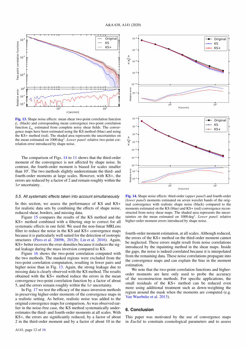
In this section we study the effect of the shape noise on conver-gence maps. We derived noisy shear maps, assuming a Gaus-sian noise (σε = 0.3). Then, we compared the two mass-inversion methods. The pixel difference cannot be used in thiscase because the convergence maps are noise dominated (seeFig. 3, upper right panel). However, we can still assess the qual-ity of the convergence maps using two-point correlation func-tions because the ellipticity correlation is an unbiased estimateof the shear correlation, and similarly, the convergence two-pointcorrelation functions is unbiased by the shape noise.

Figure 13 compares the results of the KS and KS+ methodswhen shape noise is included. Compared to Fig. 10, the two-point correlation of the noisy maps is less smooth because thenoise fluctuations do not completely average out. However, theamplitude of the errors introduced by the mass inversion remainremarkably similar to the errors computed without shape noisefor the KS and KS+ methods. The same conclusions then hold:the errors are about five times smaller with the KS+ method.

Moments of noisy maps are biased and potentially domi-nated by the shape noise contribution. For instance, the total vari-ance in the noisy convergence map is expected to be the sum ofthe variance in the noise-free convergence map and the noisevariance. Therefore moments of the noisy KS and KS+ con-vergence maps cannot be directly compared to moments of theoriginal noise-free convergence maps. Instead, Fig. 14 comparesthem to the moments of the original convergence maps wherenoise was added with properties similar to the noise expectedin the convergence maps. For this purpose, we generated noisemaps N1 and N2 for each field using Eqs. (11) and (12), andwe derived the noise to be added in the convergence usingEq. (14).

A141, page 11 of 16

A&A 638, A141 (2020)

10-6

10-5

10-4

Tw

o-p

oin

t co

rrela

tion f

unct

ions

OriginalKSKS+

101 102

θ [arcmin]

10-2

10-1

100

Rela

tive e

rror

Fig. 13. Shape noise effects: mean shear two-point correlation functionξ+ (black) and corresponding mean convergence two-point correlationfunction ξκE estimated from complete noisy shear fields. The conver-gence maps have been estimated using the KS method (blue) and usingthe KS+ method (red). The shaded area represents the uncertainties onthe mean estimated on 1000 deg2. Lower panel: relative two-point cor-relation error introduced by shape noise.

The comparison of Figs. 14 to 11 shows that the third-ordermoment of the convergence is not affected by shape noise. Incontrast, the fourth-order moment is biased for scales smallerthan 10′. The two methods slightly underestimate the third- andfourth-order moments at large scales. However, with KS+, theerrors are reduced by a factor of 2 and remain roughly within the1σ uncertainty.

5.5. All systematic effects taken into account simultaneously

In this section, we assess the performance of KS and KS+for realistic data sets by combining the effects of shape noise,reduced shear, borders, and missing data.

Figure 15 compares the results of the KS method and theKS+ method combined with a filtering step to correct for allsystematic effects in one field. We used the non-linear MRLensfilter to reduce the noise in the KS and KS+ convergence mapsbecause it is particularly well suited for the detection of isotropicstructures (Pires et al. 2009b, 2012b; Lin et al. 2016). Again,KS+ better recovers the over-densities because it reduces the sig-nal leakage during the mass inversion compared to KS.

Figure 16 shows the two-point correlation computed withthe two methods. The masked regions were excluded from thetwo-point correlation computation, resulting in fewer pairs andhigher noise than in Fig. 13. Again, the strong leakage due tomissing data is clearly observed with the KS method. The resultsobtained with the KS+ method reduce the errors in the meanconvergence two-point correlation function by a factor of about5, and the errors remain roughly within the 1σ uncertainty.

In Fig. 17 we test the efficacy of the mass-inversion methodsin preserving higher-order moments of the convergence maps ina realistic setting. As before, realistic noise was added to theoriginal convergence maps for comparison. As was observed ear-lier in the noise-free case, the KS method systematically under-estimates the third- and fourth-order moments at all scales. WithKS+, the errors are significantly reduced, by a factor of about2 in the third-order moment and by a factor of about 10 in the

10 10

10 9

10 8

10 7

10 6

<3 E

>

OriginalKSKS+

101 102

[arcmin]

10 1

Rela

tive

erro

r

10 12

10 11

10 10

10 9

10 8

10 7

10 6

<4 E

>

OriginalKSKS+

101 102

[arcmin]

10 2

10 1

Rela

tive

erro

r

Fig. 14. Shape noise effects: third-order (upper panel) and fourth-order(lower panel) moments estimated on seven wavelet bands of the orig-inal convergence with realistic shape noise (black) compared to themoments estimated on the KS (blue) and KS+ (red) convergence recon-structed from noisy shear maps. The shaded area represents the uncer-tainties on the mean estimated on 1000 deg2. Lower panel: relativehigher-order moment errors introduced by shape noise.

fourth-order moment estimation, at all scales. Although reduced,the errors of the KS+ method on the third-order moment cannotbe neglected. These errors might result from noise correlationsintroduced by the inpainting method in the shear maps. Insidethe gaps, the noise is indeed correlated because it is interpolatedfrom the remaining data. These noise correlations propagate intothe convergence maps and can explain the bias in the momentestimation.

We note that the two-point correlation functions and higher-order moments are here only used to probe the accuracyof the reconstruction methods. For specific applications, thesmall residuals of the KS+ method can be reduced evenmore using additional treatment such as down-weighting theregion around the mask when the moments are computed (e.g.Van Waerbeke et al. 2013).

6. Conclusion

This paper was motivated by the use of convergence mapsin Euclid to constrain cosmological parameters and to assess

A141, page 12 of 16

S. Pires et al.: Euclid: Reconstruction of weak-lensing mass maps for non-Gaussianity studies

0 200 400 600 800 1000x [pixels]

0

200

400

600

800

1000

y [pixels]

−0.05

0.00

0.05

0.10

0.15

0.20

0.25

0.30

0.35

0.40

0 200 400 600 800 1000x [pixels]

0

200

400

600

800

1000

y [pixels]

0.0

0.1

0.2

0.3

0.4

0.5

0.6

0.7

0.8

0.9

1.0

0 200 400 600 800 1000x [pixels]

0

200

400

600

800

1000

y [pixels]

−0.05

0.00

0.05

0.10

0.15

0.20

0.25

0.30

0.35

0.40

0 200 400 600 800 1000x [pixels]

0

200

400

600

800

1000

y [pixels]

−0.05

0.00

0.05

0.10

0.15

0.20

0.25

0.30

0.35

0.40

Fig. 15. All systematic effects: upper panels: original E-mode convergence κ map (left) and the mask that is applied to the shear maps (right).Lower panels: convergence map reconstructed from an incomplete noisy shear field using the KS method (left) and using the KS+ method (right)applying a non-linear MRLens filtering with αFDR = 0.05. The field is 10 × 10 downsampled to 1024 × 1024 pixels.

10-6

10-5

10-4

Tw

o-p

oin

t co

rrela

tion f

unct

ions

OriginalKSKS+

101 102

θ [arcmin]

10-2

10-1

100

Rela

tive e

rror

Fig. 16. All systematic effects: mean shear two-point correlationfunction ξ+ (black) and corresponding mean convergence two-pointcorrelation function ξκE estimated from incomplete noisy shear fields.The convergence maps have been estimated using KS (blue) and KS+(red). The convergence two-point correlations were estimated outsidethe mask. The shaded area represents the uncertainties on the meanestimated on 1000 deg2. Lower panel: normalised difference betweenthe two upper curves.

other physical constraints. Convergence maps encode the lens-ing information in a different manner, allowing more optimisedcomputations than shear. However, the mass-inversion process issubject to field border effects, missing data, reduced shear, intrin-sic alignments, and shape noise. This requires accurate controlof the systematic effects during the mass inversion to reducethe information loss as much as possible. We presented andcompared the two mass-inversion methods that are included inthe official Euclid data-processing pipeline: the standard Kaiser& Squires (KS) method, and an improved Kaiser & Squires(KS+) mass-inversion technique that integrates corrections forthe mass-mapping systematic effects. The systematic effectson the reconstructed convergence maps were studied using theEuclid Flagship mock galaxy catalogue.

In a first step, we analysed and quantified one by one the sys-tematic effects on reconstructed convergence maps using two-point correlation functions and moments of the convergence. Inthis manner, we quantified the contribution of each effect to theerror budget to better understand the error distribution in the con-vergence maps. With KS, missing data are the dominant effect atall scales. Field border effects also have a strong effect, but onlyat the map borders. These two effects are significantly reducedwith KS+. The reduced shear is the smallest effect in terms ofcontribution and only affects small angular scales. The study alsoshowed that pixellisation provides an intrinsic regularisation andthat no additional smoothing step is required to avoid infinitenoise in the convergence maps.

A141, page 13 of 16

A&A 638, A141 (2020)

10 10

10 9

10 8

10 7

10 6

<3 E

>

OriginalKSKS+

101 102

[arcmin]

10 1Rela

tive

erro

r

10 12

10 11

10 10

10 9

10 8

10 7

<4 E

>

OriginalKSKS+

101 102

[arcmin]

10 2

10 1

Rela

tive

erro

r

Fig. 17. All systematic effects: third-order (upper panel) and fourth-order (lower panel) moments estimated on seven wavelet bands ofthe original convergence with realistic noise (black) compared to themoments estimated using KS (blue) and KS+ (red) obtained fromincomplete noisy shear maps. The third- and fourth-order moments areestimated outside the mask. The shaded area represents the uncertaintieson the mean estimated on 1000 deg2. Lower panel: relative higher-ordermoment errors.

In a second step, we quantified the errors introduced by theKS and KS+ methods in a realistic setting that included the sys-tematic effects. We showed that the KS+ method reduces theerrors on the two-point correlation functions and on the momentsof the convergence compared to the KS method. The errorsintroduced by the mass inversion on the two-point correlationof the convergence maps are reduced by a factor of about 5.The errors on the third-order and fourth-order moment estimatesare reduced by factors of about 2 and 10, respectively. Someerrors remain in the third-order moment that remain within the2σ uncertainty. They might result from noise correlations intro-duced by the inpainting method inside the gaps.

Our study was conducted on a mock of 1000 deg2 dividedinto ten fields of 10 × 10 to remain in the flat-sky approxima-tion. Euclid will observe a field of 15 000 deg2. As long as KS+has not been extended to the curved sky, it is not possible toapply the method to larger fields without introducing significantprojection effects. However, the Euclid survey can be dividedinto small fields, which allows reducing the uncertainties in the

statistics that are estimated on the convergence maps. Moreover,we can expect that part of the errors will average out.

Recent studies have shown that combining the shear two-point statistics with higher-order statistics of the conver-gence such as higher-order moments (Vicinanza et al. 2018),Minkowski functionals (Vicinanza et al. 2019), or peak counts(Liu et al. 2015; Martinet et al. 2018) allows breaking commondegeneracies. The precision of the KS+ mass inversion makesthe E-mode convergence maps a promising tool for such cos-mological studies. In future work, we plan to propagate theseerrors into cosmological parameter constraints using higher-order moments and peak counts.

Acknowledgements. This study has been carried inside the Mass MappingWork Package of the Weak Lensing Science Working Group of the Euclidproject to better understand the impact of the mass inversion systematic effectson the convergence maps. The authors would like to thank the referees for theirvaluable comments, which helped to improve the manuscript. S. Pires thanksF. Sureau, J. Bobin, M. Kilbinger, A. Peel and J.-L. Starck for useful discus-sions. The Euclid Consortium acknowledges the European Space Agency andthe support of a number of agencies and institutes that have supported thedevelopment of Euclid. A detailed complete list is available on the Euclid website (http://www.euclid-ec.org). In particular the Academy of Finland, theAgenzia Spaziale Italiana, the Belgian Science Policy, the Canadian Euclid Con-sortium, the Centre National d’Etudes Spatiales, the Deutsches Zentrum für Luft-and Raumfahrt, the Danish Space Research Institute, the Fundação para a Ciêncae a Tecnologia, the Ministerio de Economia y Competitividad, the NationalAeronautics and Space Administration, the Netherlandse Onderzoekschool VoorAstronomie, the Norvegian Space Center, the Romanian Space Agency, the StateSecretariat for Education, Research and Innovation (SERI) at the Swiss SpaceOffice (SSO), and the United Kingdom Space Agency.

ReferencesBartelmann, M. 1995, A&A, 303, 643Bartelmann, M., & Schneider, P. 2001, Phys. Rep., 340, 291Benabed, K., & Scoccimarro, R. 2006, A&A, 456, 421Benjamini, Y., & Hochberg, Y. 1995, J. R. Stat. Soc. B, 57, 289Bernardeau, F., Colombi, S., Gaztañaga, E., & Scoccimarro, R. 2002a, Phys.

Rep., 367, 1Bernardeau, F., Mellier, Y., & van Waerbeke, L. 2002b, A&A, 389, L28Bridle, S. L., Hobson, M. P., Lasenby, A. N., & Saunders, R. 1998, MNRAS,

299, 895Chang, C., Vikram, V., Jain, B., et al. 2015, Phys. Rev. Lett., 115, 051301Chang, C., Pujol, A., Mawdsley, B., et al. 2018, MNRAS, 475, 3165Crittenden, R. G., Natarajan, P., Pen, U.-L., & Theuns, T. 2002, ApJ, 568, 20Crocce, M., Castander, F. J., Gaztañaga, E., Fosalba, P., & Carretero, J. 2015,

MNRAS, 453, 1513Cropper, M., Hoekstra, H., Kitching, T., et al. 2013, MNRAS, 431, 3103Elad, M., Starck, J.-L., Querre, P., & Donoho, D. J. 2005, Appl. Comput.

Harmonic Anal., 19, 340Fosalba, P., Gaztañaga, E., Castander, F. J., & Manera, M. 2008, MNRAS, 391,

435Fosalba, P., Gaztañaga, E., Castander, F. J., & Crocce, M. 2015, MNRAS, 447,

1319Green, J., Schechter, P., & Baltay, C. 2012, ArXiv e-prints [arXiv:1208.4012]Hildebrandt, H., Choi, A., Heymans, C., et al. 2016, MNRAS, 463, 635Jeffrey, N., Abdalla, F.B., Lahav, O., et al. 2018, MNRAS, 479, 2871Joachimi, B., Semboloni, E., Hilbert, S., et al. 2013, MNRAS, 436, 819Jullo, E., Pires, S., Jauzac, M., & Kneib, J.-P. 2014, MNRAS, 437, 3969Kaiser, N. 1995, ApJ, 439, L1Kaiser, N., & Squires, G. 1993, ApJ, 404, 441Kilbinger, M., Bonnett, C., & Coupon, J. 2014, Athena: Tree code for second-

order correlation functions, Astrophysics Source Code LibraryKilbinger, M., & Schneider, P. 2005, A&A, 442, 69Lanusse, F., Starck, J.-L., Leonard, A., & Pires, S. 2016, A&A, 591, A2Laureijs, R., Amiaux, J., & Arduini, S. 2011, ArXiv e-prints [arXiv:1110.3193]Leauthaud, A., Massey, R., Kneib, J.-P., et al. 2007, ApJS, 172, 219Leonard, A., Pires, S., & Starck, J.-L. 2012, MNRAS, 423, 3405Lin, C.-A., Kilbinger, M., & Pires, S. 2016, A&A, 593, A88Liu, J., Petri, A., Haiman, Z., et al. 2015, Phys. Rev. D, 91, 063507LSST Science Collaboration (Abell, P.A., et al.) 2009, ArXiv e-prints

[arXiv:0912.0201]

A141, page 14 of 16

S. Pires et al.: Euclid: Reconstruction of weak-lensing mass maps for non-Gaussianity studies

Marshall, P. J., Hobson, M. P., Gull, S. F., & Bridle, S. L. 2002, MNRAS, 335,1037

Martinet, N., Schneider, P., Hildebrandt, H., et al. 2018, MNRAS, 474, 712Massey, R., Rhodes, J., Ellis, R., et al. 2007, Nature, 445, 286Oguri, M., Miyazaki, S., Hikage, C., et al. 2018, PASJ, 70, S26Pichon, C., Thiébaut, E., Prunet, S., et al. 2010, MNRAS, 401, 705Pires, S., Starck, J.-L., Amara, A., et al. 2009a, MNRAS, 395, 1265Pires, S., Starck, J.-L., Amara, A., Réfrégier, A., & Teyssier, R. 2009b, A&A,

505, 969Pires, S., Plaszczynski, S., & Lavabre, A. 2012a, Stat. Method., 9, 71Pires, S., Leonard, A., & Starck, J.-L. 2012b, MNRAS, 423, 983Potter, D., Stadel, J., & Teyssier, R. 2017, Comput. Astrophys. Cosmol., 4, 2Schneider, P. 1995, A&A, 302, 639Schneider, P. 1996, MNRAS, 283, 837Schneider, P., van Waerbeke, L., Mellier, Y., et al. 1998, A&A, 333, 767Schneider, P., van Waerbeke, L., Kilbinger, M., & Mellier, Y. 2002, A&A,

396, 1Schrabback, T., Hilbert, S., Hoekstra, H., et al. 2015, MNRAS, 454, 1432Schrabback, T., Schirmer, M., van der Burg, R. F. J., et al. 2018, A&A, 610, A85Seitz, C., & Schneider, P. 1995, A&A, 297, 287Seitz, S., & Schneider, P. 1996, A&A, 305, 383Seitz, S., & Schneider, P. 2001, A&A, 374, 740Seitz, S., Schneider, P., & Bartelmann, M. 1998, A&A, 337, 325Seljak, U. 1998, ApJ, 506, 64Shan, H. Y., Kneib, J.-P., Comparat, J., et al. 2014, MNRAS, 442, 2534Shapiro, C. 2009, ApJ, 696, 775Shi, X., Schneider, P., & Joachimi, B. 2011, A&A, 533, A48Squires, G., & Kaiser, N. 1996, ApJ, 473, 65Starck, J.-L., & Murtagh, F. 2002, Astronomical Image and Data Analysis

(Springer-Verlag)Starck, J.-L., Murtagh, F., & Bijaoui, A. 1998, Image Processing and Data

Analysis: The Multiscale Approach (Cambridge University Press)Starck, J.-L., Pires, S., & Réfrégier, A. 2006, A&A, 451, 1139Van Waerbeke, L., Benjamin, J., Erben, T., et al. 2013, MNRAS, 433, 3373Vicinanza, M., Cardone, V. F., Maoli, R., Scaramella, R., & Er, X. 2018, Phys.

Rev. D, 97, 023519Vicinanza, M., Cardone, V. F., Maoli, R., et al. 2019, Phys. Rev. D, 99, 043534Vikram, V., Chang, C., Jain, B., et al. 2015, Phys. Rev. D, 92, 022006White, M. 2005, Astropart. Phys., 23, 349Xavier, H. S., Abdalla, F. B., & Joachimi, B. 2016, MNRAS, 459, 3693

1 Université Paris Diderot, AIM, Sorbonne Paris Cité, CEA, CNRS,91191 Gif-sur-Yvette Cedex, Francee-mail: sandrine.pires@cea.fr

2 Universitäts-Sternwarte München, Fakultät für Physik, Ludwig-Maximilians-Universität München, Scheinerstrasse 1, 81679München, Germany

3 Max Planck Institute for Extraterrestrial Physics, Giessenbachstr. 1,85748 Garching, Germany

4 INAF-Osservatorio Astrofisico di Torino, Via Osservatorio 20,10025 Pino Torinese (TO), Italy

5 INAF-Osservatorio Astrofisico di Torino, Via Osservatorio 20,10025 Pino Torinese (TO), Italy

6 APC, AstroParticule et Cosmologie, Université Paris Diderot,CNRS/IN2P3, CEA/lrfu, Observatoire de Paris, Sorbonne ParisCité, 10 rue Alice Domon et Léonie Duquet, 75205 Paris Cedex 13,France

7 Instituto de Astrofísica e Ciências do Espaço, Universidade doPorto, CAUP, Rua das Estrelas, 4150-762 Porto, Portugal

8 Institut de Física d’Altes Energies IFAE, 08193 Bellaterra,Barcelona, Spain

9 INAF-Osservatorio Astronomico di Roma, Via Frascati 33, 00078Monteporzio Catone, Italy

10 Department of Physics “E. Pancini”, University Federico II, ViaCinthia 6, 80126 Napoli, Italy

11 INFN section of Naples, Via Cinthia 6, 80126 Napoli, Italy12 INAF-Osservatorio Astronomico di Capodimonte, Via Moiariello

16, 80131 Napoli, Italy13 Centre National d’Etudes Spatiales, Toulouse, France14 Institute for Astronomy, University of Edinburgh, Royal Observa-

tory, Blackford Hill, Edinburgh EH9 3HJ, UK15 ESAC/ESA, Camino Bajo del Castillo, s/n., Urb. Villafranca del

Castillo, 28692 Villanueva de la Cañada, Madrid, Spain16 Department of Astronomy, University of Geneva, Ch. d’Écogia 16,

1290 Versoix, Switzerland17 Institute of Space Sciences (ICE, CSIC), Campus UAB, Carrer de

Can Magrans, s/n, 08193 Barcelona, Spain18 Institut d’Estudis Espacials de Catalunya (IEEC), 08034 Barcelona,

Spain19 INAF-Osservatorio Astronomico di Trieste, Via G. B. Tiepolo 11,

34131 Trieste, Italy20 INAF-Osservatorio di Astrofisica e Scienza dello Spazio di Bologna,

Via Piero Gobetti 93/3, 40129 Bologna, Italy21 INAF-IASF Milano, Via Alfonso Corti 12, 20133 Milano, Italy22 von Hoerner & Sulger GmbH, SchloßPlatz 8, 68723 Schwetzingen,

Germany23 Aix-Marseille Univ, CNRS/IN2P3, CPPM, Marseille, France24 Institute for Computational Science, University of Zurich, Win-

terthurerstrasse 190, 8057 Zurich, Switzerland25 Institut de Physique Nucléaire de Lyon, 4 rue Enrico Fermi, 69622

Villeurbanne Cedex, France26 Université de Genève, Département de Physique Théorique and

Centre for Astroparticle Physics, 24 quai Ernest-Ansermet, 1211Genève 4, Switzerland

27 Institute of Theoretical Astrophysics, University of Oslo, PO Box1029, Blindern 0315, Oslo, Norway

28 Argelander-Institut für Astronomie, Universität Bonn, Auf demHügel 71, 53121 Bonn, Germany

29 Centre for Extragalactic Astronomy, Department of Physics,Durham University, South Road, Durham DH1 3LE, UK

30 Observatoire de Sauverny, Ecole Polytechnique Fédérale de Lau-sanne, 1290 Versoix, Switzerland

31 Jet Propulsion Laboratory, California Institute of Technology, 4800Oak Grove Drive, Pasadena, CA 91109, USA

32 Dipartimento di Fisica e Astronomia, Universitá di Bologna, ViaGobetti 93/2, 40129 Bologna, Italy

33 Institute of Space Sciences (IEEC-CSIC), c/Can Magrans s/n, 08193Cerdanyola del Vallés, Barcelona, Spain

34 Centro de Investigaciones Energéticas, Medioambientales y Tec-nológicas (CIEMAT), Avenida Complutense 40, 28040 Madrid,Spain

35 Instituto de Astrofísica e Ciências do Espaço, Faculdade de Ciên-cias, Universidade de Lisboa, Tapada da Ajuda, 1349-018 Lisboa,Portugal

36 Departamento de Física, Faculdade de Ciências, Universidade deLisboa, Edifício C8, Campo Grande, 1749-016 Lisboa, Portugal

37 Universidad Politécnica de Cartagena, Departamento de Electrónicay Tecnología de Computadoras, 30202 Cartagena, Spain

38 Infrared Processing and Analysis Center, California Institute ofTechnology, Pasadena, CA 91125, USA

A141, page 15 of 16

A&A 638, A141 (2020)

Appendix A: KS+ inpainting algorithm

This appendix describes the KS+ method presented in Sect. 3 inmore detail. The solution of the KS+ mass inversion is obtainedthrough the iterative algorithm described in Algorithm 1.

The outer loop starting at step 5 is used to correct for thereduced shear using the iterative scheme described in Sect. 3.3.The inner loop starting at step 7 is used to solve the optimisa-tion problem defined by Eq. (17). Φ is the discrete cosine trans-form operator matrix. If the convergence κ is sparse in Φ, mostof the signal is contained in the strongest DCT coefficients. Thesmallest coefficients result from missing data, border effects, andshape noise. Thus, the algorithm is based on an iterative algo-rithm with a threshold that decreases exponentially (at each iter-ation) from a maximum value to zero, following the decreasinglaw F described in Pires et al. (2009a). By accumulating increas-ingly more high DCT coefficients through each iteration, thegaps in γ fill up steadily, and the power of the spurious B modesdue to the gaps decreases. The algorithm uses the fast Fouriertransform at each iteration to compute the shear maps γ from theconvergence maps κ (step 14) and the inverse relation (step 16).

A data-driven power spectrum prior is introduced atsteps 11–13. To do so, the KS+ algorithm uses the undecimatedisotropic wavelet transform that decomposes an image κ into aset of coefficients w1,w2, . . . ,wJ , cJ , as a superposition of theform

κ[i1, i2] = cJ [i1, i2] +

J∑j=1

w j[i1, i2], (A.1)

where cJ is a smoothed version of the image, and κ and w j are aset of aperture mass maps (usually called wavelet bands) at scaleθ = 2 j. Then, we estimate the variance on each wavelet band w j.The variance per scale estimated in this way can be directly com-pared to the power spectrum. This provides a way to estimate abroadband power spectrum of the convergence κ from incom-plete data. The power spectrum is then enforced by multiplyingeach wavelet coefficient by the factor σout

j /σinj inside the gaps,

where σinj and σout

j are the standard deviation estimated in thewavelet band w j inside and outside the mask, respectively. This

normalisation can be described by a linear operator Q as used inEq. (17). The constraint is applied on the E- and B-mode com-ponents before reconstructing the convergence κ by backwardwavelet transform.

Algorithm 1 KS+ algorithm1. Project the shear from the celestial sphere onto a tangent

plane by projecting the galaxy positions and applying a localrotation to the shear field.

2. Bin the projected shear onto a grid and define γ as the aver-age shear in each pixel.

3. Set the mask M: M[i1, i2] = 1 for pixels where we have infor-mation and M[i1, i2] = 0 for pixels with no galaxies, and takea support twice larger for the shear maps and include the bor-ders in the masked region (see Fig. 1).

4. Set the maximum number of iterations to Imax = 100, themaximum threshold λmax = max(| ΦTP∗γ |), and the mini-mum threshold λmin = 0.

5. Set k = 0, κkE

= 0 and iterate:6. Update the shear γk = γ (1 − κk

E) and initialise the solu-

tion to κk = P∗γk.7. Set i = 0, λ0 = λmax, κi = κk and iterate:

8. Compute the forward transform: α = ΦTκi.9. Compute α by setting to zero the coefficients α

below the threshold λi.10. Reconstruct κi from α: κi = Φα.11. Decompose κi into its wavelet coefficientsw1,w2, . . . ,wJ , cJ .

12. Renormalise the wavelet coefficients w j by a factorσout

j /σinj inside the gaps.

13. Reconstruct κi by performing the backward wavelettransform from the normalised coefficients.

14. Perform the inverse mass relation: γi = Pκi.15. Enforce the observed shear γ outside the gaps: γi =

(1 −M)γi + Mγk.16. Perform the direct mass inversion: κi = P∗γi.17. Update the threshold: λi = F(i, λmin, λmax).18. Set i = i + 1. If i < Imax, return to step 8.

19. Set k = k + 1, κk = κi. If k < 3, return to step 6.

A141, page 16 of 16