Eulerian â€” Eulerian Large Eddy Simulations Applied to Non

This paper is a part of the hereunder thematic dossierpublished in OGST Journal, Vol. 69, No. 1, pp. 3-188

and available online hereCet article fait partie du dossier thématique ci-dessouspublié dans la revue OGST, Vol. 69, n°1, pp. 3-188

et téléchargeable ici

Do s s i e r

DOSSIER Edited by/Sous la direction de : C. Angelberger

IFP Energies nouvelles International Conference / Les Rencontres Scientifiques d’IFP Energies nouvelles

LES4ICE 2012 - Large Eddy Simulation for Internal Combustion Engine FlowsLES4ICE 2012 - La simulation aux grandes échelles pour les écoulements

dans les moteurs à combustion interneOil & Gas Science and Technology – Rev. IFP Energies nouvelles, Vol. 69 (2014), No. 1, pp. 3-188

Copyright © 2014, IFP Energies nouvelles

3> Editorial

11> Boundary Conditions and SGS Models for LES of Wall-BoundedSeparated Flows: An Application to Engine-Like GeometriesConditions aux limites et modèles SGS pour les simulations LESd’écoulements séparés délimités par des parois : une applicationaux géométries de type moteurF. Piscaglia, A. Montorfano, A. Onorati and F. Brusiani

29> LES of Gas Exchange in IC EnginesLES échanges gazeux pour moteurs à combustion interneV. Mittal, S. Kang, E. Doran, D. Cook and H. Pitsch

41> Evaluating Large-Eddy Simulation (LES) and High-Speed ParticleImage Velocimetry (PIV) with Phase-Invariant Proper OrthogonalDecomposition (POD)Évaluation de données de simulation aux grandes échelles (LES) et devélocimétrie par imagerie de particules (PIV) via une décompositionorthogonale aux valeurs propres invariante en phase (POD)P. Abraham, K. Liu, D. Haworth, D. Reuss and V. Sick

61> Large Eddy Simulation (LES) for IC Engine FlowsSimulations des grandes échelles et écoulements dans les moteursà combustion interneT.-W. Kuo, X. Yang, V. Gopalakrishnan and Z. Chen

83> Numerical Methods and Turbulence Modeling for LES of PistonEngines: Impact on Flow Motion and CombustionMéthodes numériques et modèles de turbulence pour la LES de moteursà pistons : impact sur l’aérodynamique et la combustionA. Misdariis, A. Robert, O. Vermorel, S. Richard and T. Poinsot

107 > Investigation of Boundary Condition and Field Distribution Effects on theCycle-to-Cycle Variability of a Turbocharged GDI Engine Using LES

Études des effets des conditions aux limites et de la distribution deschamps sur la variabilité cycle-à-cycle dans un moteur GDIturbocompressé en utilisant la LESS. Fontanesi, S. Paltrinieri, A. D'Adamo and S. Duranti

129 > Application of LES for Analysis of Unsteady Effects on CombustionProcesses and Misfi res in DISI EngineApplication de simulation aux grandes échelles pour l’analyse deseffets instationnaires de combustion et d’allumage raté dansles moteurs DISID. Goryntsev, K. Nishad, A. Sadiki and J. Janicka

141 > Eulerian – Eulerian Large Eddy Simulations Applied toNon-Reactive Transient Diesel SpraysÉvaluation de la méthode Euler – Euler pour la simulation auxgrandes échelles de sprays Diesel instationnaires non-réactifsA. Robert, L. Martinez, J. Tillou and S. Richard

155 > Large-Eddy Simulation of Diesel Spray Combustion with ExhaustGas RecirculationSimulation aux grandes échelles de la combustion d’un spray Dieselpour différents taux d’EGRJ. Tillou, J.-B. Michel, C. Angelberger, C. Bekdemir and D. Veynante

167 > Modeling of EGR Mixing in an Engine Intake Manifold Using LESModélisation du mélange de EGR dans la tubulure d’admissionà l’aide de la technique de LESA. Sakowitz, S. Reifarth, M. Mihaescu and L. Fuchs

177 > LES of the Exhaust Flow in a Heavy-Duty EngineLES de l’écoulement d’échappement dans un moteur de camionO. Bodin, Y. Wang, M. Mihaescu and L. Fuchs

©Ph

otos:

DOI:

10.25

16/og

st/20

1313

9,IF

PEN,

X

http://ogst.ifpenergiesnouvelles.fr/articles/ogst/abs/2014/01/contents/contents.html


IFP Energies nouvelles International ConferenceRencontres Scientifiques d'IFP Energies nouvelles

LES4ICE 2012 - Large Eddy Simulation for Internal Combustion Engine FlowsLES4ICE 2012 - La simulation aux grandes échelles pour les écoulements dans les moteurs à combustion interne

Eulerian – Eulerian Large Eddy Simulations Applied

to Non-Reactive Transient Diesel Sprays

Anthony Robert, Lionel Martinez, Julien Tillou and Stéphane Richard*

IFP Energies nouvelles, 1-4 avenue de Bois-Préau, 92852 Rueil-Malmaison - Francee-mail: [email protected]

* Corresponding author

Resume— Evaluation de la methode Euler – Euler pour la simulation aux grandes echelles de sprays

Diesel instationnaires non-reactifs — L’objectif de cette etude est de realiser et d’analyser des

simulations aux grandes echelles (LES, Large Eddy Simulations) de sprays Diesel

instationnaires dans une cellule haute pression et haute temperature. Pour representer les

strategies d’injection d’un moteur Diesel actuel, deux cas sont analyses : le premier est une

mono-injection, et une double injection est ensuite simulee. Pour chaque configuration,

plusieurs realisations sont calculees pour obtenir les valeurs moyennes et les fluctuations de

concentration en carburant. Une sensibilite au maillage est realisee pour juger de la qualite du

maillage en comparant les profils numeriques de fraction massique de carburant aux profils

experimentaux. Cette comparaison est egalement etendue aux penetrations vapeur et aux

angles de sprays. Ensuite, l’influence sur les resultats numeriques de la condition limite

d’injection, du profil de taux d’introduction, ainsi que du retard a l’injection sont evalues.

Pour finir, des recommandations pour les futures simulations LES de sprays instationnaires en

moteur Diesel sont suggerees.

Abstract— Eulerian – Eulerian Large Eddy Simulations Applied to Non-Reactive Transient Diesel

Sprays — The aim of this study is to perform and analyze LES (Large Eddy Simulations) simula-

tions of transient Diesel sprays in a high-pressure and high-temperature vessel. In order to be repre-

sentative of real Diesel injection strategies, two cases are investigated: the first one corresponds to a

single injection, while a double injection is performed in the second case. For each case, numerous

realizations are computed to retrieve average values and fluctuations of fuel concentration. A mesh

refinement sensitivity analysis is conducted to assess the quality of the LES by comparing numerical

fuel mass fraction profiles with experimental ones. This comparison is then extended to spray angles

and vapor penetrations. The influence of injection boundary conditions such as injection rate profile

and injection delay, on transient LES results is then evaluated. Finally, guidelines for simulating

transient Diesel sprays in engines with LES are proposed.

Oil & Gas Science and Technology – Rev. IFP Energies nouvelles, Vol. 69 (2014), No. 1, pp. 141-154Copyright � 2013, IFP Energies nouvellesDOI: 10.2516/ogst/2013140

http://ogst.ifpenergiesnouvelles.fr/

http://ifpenergiesnouvelles.fr/


INTRODUCTION

In the past few years, Large Eddy Simulation (LES) has

known a growing interest from the automotive commu-

nity because of its unique capability to reproduce

unsteady and sporadic phenomena like Cycle-to-Cycle

Variations (CCV) [1-4] or abnormal combustions [5] in

Spark Ignition (SI) engines. In the Diesel context, LES

may be used to better predict pollutant emissions such

as soots, which are highly dependent on the local air-fuel

mixing process, and their CCV or to study transient

operations like cold starts. However, up to now, such

engineering issues were not properly addressed by

LES, notably because detailed spray models and valida-

tions were needed.

A specificity of Diesel injection is that thermodynamic

conditions are severe (injection pressure up to 2 500 bar)

and that the introduction rate is often split into several

sub-injections, leading to highly unsteady behaviours.

However, most of preceding works on LES of Diesel

sprays [6-11] were oriented towards quasi-steady behav-

iours in very long injection cases, also neglecting injec-

tion to injection variability effects. Therefore,

dedicated studies have to be performed to assess the abil-

ity of LES models to correctly predict spray evolutions

and cyclic variations in more realistic Diesel conditions.

The objective of this work is to perform detailed LES

validations of transient Diesel sprays using the Eulerian-

Eulerian approach developed by Simonin [12] and by

Fevrier et al. [13] and further adapted to engine condi-

tions by Martinez et al. [6, 14, 15]. For this purpose, ded-

icated experiments conducted at IFP Energies nouvelles

in a high pressure vessel are used. Single and double

injections are simulated, and comparisons are made with

experimental fuel concentration profiles as well as pene-

tration lengths and angles for a number of injection

events. The impact of mesh refinement or boundary con-

ditions at the injection patch is also discussed, and rec-

ommendations for future LES studies in Diesel engines

are finally drawn.

1 EXPERIMENTAL SETUP

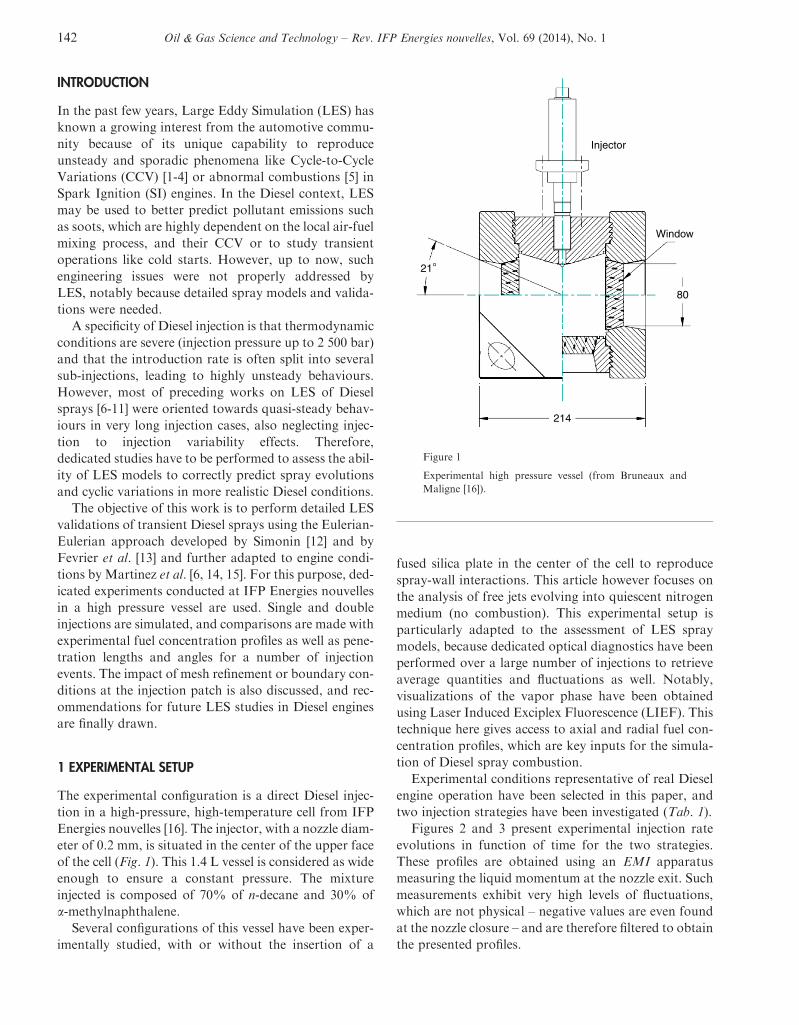
The experimental configuration is a direct Diesel injec-

tion in a high-pressure, high-temperature cell from IFP

Energies nouvelles [16]. The injector, with a nozzle diam-

eter of 0.2 mm, is situated in the center of the upper face

of the cell (Fig. 1). This 1.4 L vessel is considered as wide

enough to ensure a constant pressure. The mixture

injected is composed of 70% of n-decane and 30% of

a-methylnaphthalene.

Several configurations of this vessel have been exper-

imentally studied, with or without the insertion of a

fused silica plate in the center of the cell to reproduce

spray-wall interactions. This article however focuses on

the analysis of free jets evolving into quiescent nitrogen

medium (no combustion). This experimental setup is

particularly adapted to the assessment of LES spray

models, because dedicated optical diagnostics have been

performed over a large number of injections to retrieve

average quantities and fluctuations as well. Notably,

visualizations of the vapor phase have been obtained

using Laser Induced Exciplex Fluorescence (LIEF). This

technique here gives access to axial and radial fuel con-

centration profiles, which are key inputs for the simula-

tion of Diesel spray combustion.

Experimental conditions representative of real Diesel

engine operation have been selected in this paper, and

two injection strategies have been investigated (Tab. 1).

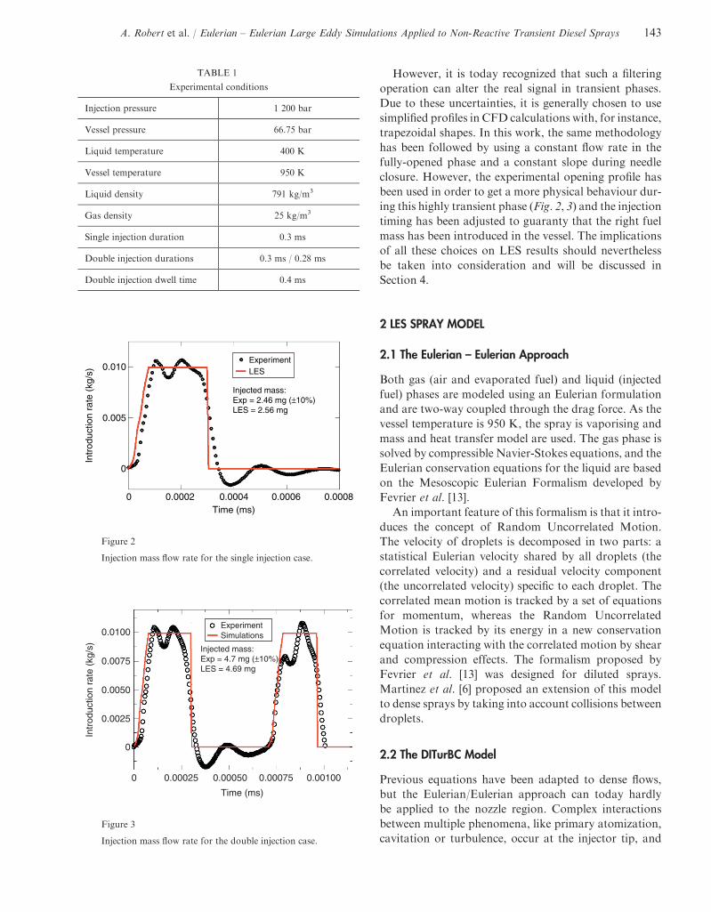
Figures 2 and 3 present experimental injection rate

evolutions in function of time for the two strategies.

These profiles are obtained using an EMI apparatus

measuring the liquid momentum at the nozzle exit. Such

measurements exhibit very high levels of fluctuations,

which are not physical – negative values are even found

at the nozzle closure – and are therefore filtered to obtain

the presented profiles.

Injector

Window

80

214

21°

Figure 1

Experimental high pressure vessel (from Bruneaux and

Maligne [16]).

142 Oil & Gas Science and Technology – Rev. IFP Energies nouvelles, Vol. 69 (2014), No. 1

However, it is today recognized that such a filtering

operation can alter the real signal in transient phases.

Due to these uncertainties, it is generally chosen to use

simplified profiles in CFD calculations with, for instance,

trapezoidal shapes. In this work, the same methodology

has been followed by using a constant flow rate in the

fully-opened phase and a constant slope during needle

closure. However, the experimental opening profile has

been used in order to get a more physical behaviour dur-

ing this highly transient phase (Fig. 2, 3) and the injection

timing has been adjusted to guaranty that the right fuel

mass has been introduced in the vessel. The implications

of all these choices on LES results should nevertheless

be taken into consideration and will be discussed in

Section 4.

2 LES SPRAY MODEL

2.1 The Eulerian – Eulerian Approach

Both gas (air and evaporated fuel) and liquid (injected

fuel) phases are modeled using an Eulerian formulation

and are two-way coupled through the drag force. As the

vessel temperature is 950 K, the spray is vaporising and

mass and heat transfer model are used. The gas phase is

solved by compressible Navier-Stokes equations, and the

Eulerian conservation equations for the liquid are based

on the Mesoscopic Eulerian Formalism developed by

Fevrier et al. [13].

An important feature of this formalism is that it intro-

duces the concept of Random Uncorrelated Motion.

The velocity of droplets is decomposed in two parts: a

statistical Eulerian velocity shared by all droplets (the

correlated velocity) and a residual velocity component

(the uncorrelated velocity) specific to each droplet. The

correlated mean motion is tracked by a set of equations

for momentum, whereas the Random Uncorrelated

Motion is tracked by its energy in a new conservation

equation interacting with the correlated motion by shear

and compression effects. The formalism proposed by

Fevrier et al. [13] was designed for diluted sprays.

Martinez et al. [6] proposed an extension of this model

to dense sprays by taking into account collisions between

droplets.

2.2 The DITurBC Model

Previous equations have been adapted to dense flows,

but the Eulerian/Eulerian approach can today hardly

be applied to the nozzle region. Complex interactions

between multiple phenomena, like primary atomization,

cavitation or turbulence, occur at the injector tip, and

0.0100

0.0075

0.0050

0.0025

0

0 0.00025 0.00050 0.00075 0.00100

Time (ms)

Intr

oduc

tion

rate

(kg

/s)

ExperimentSimulations

Injected mass:Exp = 4.7 mg (±10%)LES = 4.69 mg

Figure 3

Injection mass flow rate for the double injection case.

0.010

0.005

0.0002 0.0004 0.0006 0.0008

0

0Time (ms)

Intr

oduc

tion

rate

(kg

/s)

ExperimentLES

Injected mass:Exp = 2.46 mg (±10%)LES = 2.56 mg

Figure 2

Injection mass flow rate for the single injection case.

TABLE 1

Experimental conditions

Injection pressure 1 200 bar

Vessel pressure 66.75 bar

Liquid temperature 400 K

Vessel temperature 950 K

Liquid density 791 kg/m3

Gas density 25 kg/m3

Single injection duration 0.3 ms

Double injection durations 0.3 ms / 0.28 ms

Double injection dwell time 0.4 ms

A. Robert et al. / Eulerian – Eulerian Large Eddy Simulations Applied to Non-Reactive Transient Diesel Sprays 143

resolving all this physics would indeed necessitate addi-

tional models and very refined meshes. LES calculations

would require huge CPU costs, inaccessible to industrial

use.

A convenient way to overcome this issue was previ-

ously proposed by Martinez et al. [14], and consists in

moving the inlet boundary condition downstream from

the real injector nozzle. This approach, called model

DITurBC (Downstream Inflow Turbulent Boundary

Condition), allows to avoid computing the dense region

of the spray.

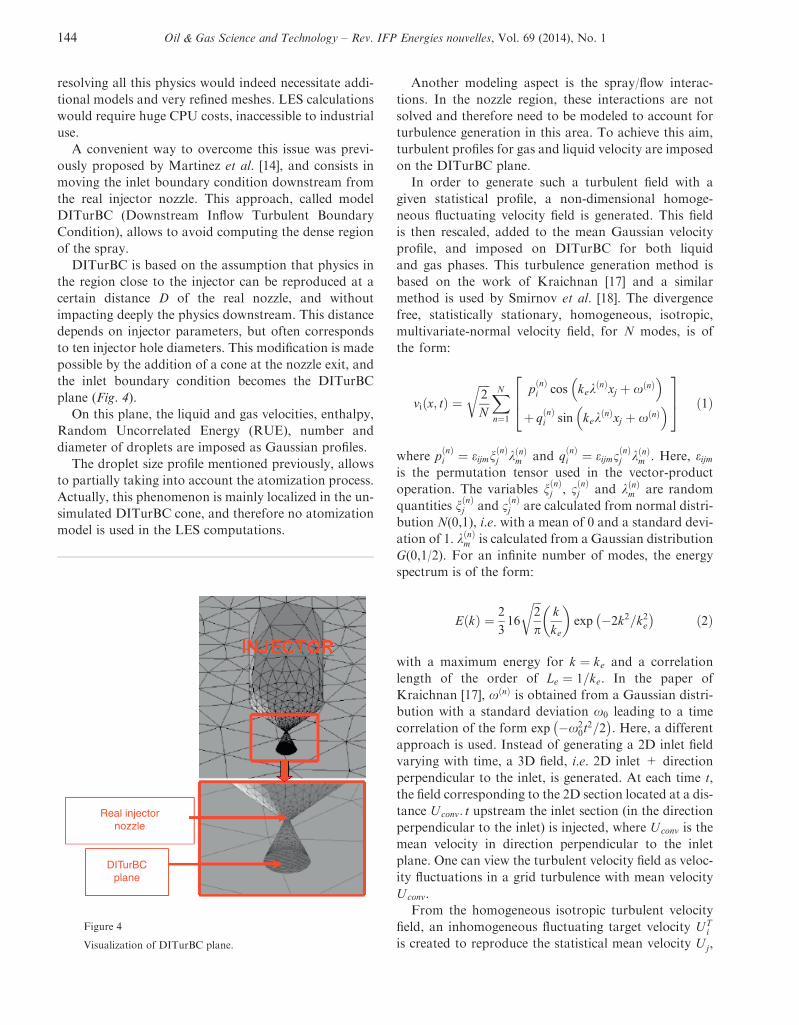
DITurBC is based on the assumption that physics in

the region close to the injector can be reproduced at a

certain distance D of the real nozzle, and without

impacting deeply the physics downstream. This distance

depends on injector parameters, but often corresponds

to ten injector hole diameters. This modification is made

possible by the addition of a cone at the nozzle exit, and

the inlet boundary condition becomes the DITurBC

plane (Fig. 4).

On this plane, the liquid and gas velocities, enthalpy,

Random Uncorrelated Energy (RUE), number and

diameter of droplets are imposed as Gaussian profiles.

The droplet size profile mentioned previously, allows

to partially taking into account the atomization process.

Actually, this phenomenon is mainly localized in the un-

simulated DITurBC cone, and therefore no atomization

model is used in the LES computations.

Another modeling aspect is the spray/flow interac-

tions. In the nozzle region, these interactions are not

solved and therefore need to be modeled to account for

turbulence generation in this area. To achieve this aim,

turbulent profiles for gas and liquid velocity are imposed

on the DITurBC plane.

In order to generate such a turbulent field with a

given statistical profile, a non-dimensional homoge-

neous fluctuating velocity field is generated. This field

is then rescaled, added to the mean Gaussian velocity

profile, and imposed on DITurBC for both liquid

and gas phases. This turbulence generation method is

based on the work of Kraichnan [17] and a similar

method is used by Smirnov et al. [18]. The divergence

free, statistically stationary, homogeneous, isotropic,

multivariate-normal velocity field, for N modes, is of

the form:

vi x; tð Þ ¼ffiffiffiffi2

N

r XNn¼1

p nð Þi cos kek

nð Þxj þ x nð Þ� �

þ q nð Þi sin kek

nð Þxj þ x nð Þ� �

264

375 ð1Þ

where p nð Þi ¼ eijmn

nð Þj k nð Þ

m and q nð Þi ¼ eijm1

nð Þj k nð Þ

m . Here, eijmis the permutation tensor used in the vector-product

operation. The variables n nð Þj , 1 nð Þ

j and k nð Þm are random

quantities n nð Þj and 1 nð Þ

j are calculated from normal distri-

bution N(0,1), i.e. with a mean of 0 and a standard devi-

ation of 1. k nð Þm is calculated from a Gaussian distribution

G(0,1/2). For an infinite number of modes, the energy

spectrum is of the form:

E kð Þ ¼ 2

316

ffiffiffi2

p

rk

ke

� �exp �2k2=k2e

� � ð2Þ

with a maximum energy for k ¼ ke and a correlation

length of the order of Le ¼ 1=ke. In the paper of

Kraichnan [17], x nð Þ is obtained from a Gaussian distri-

bution with a standard deviation x0 leading to a time

correlation of the form exp �x20t

2=2� �

. Here, a different

approach is used. Instead of generating a 2D inlet field

varying with time, a 3D field, i.e. 2D inlet + direction

perpendicular to the inlet, is generated. At each time t,

the field corresponding to the 2D section located at a dis-

tance Uconv: t upstream the inlet section (in the direction

perpendicular to the inlet) is injected, where Uconv is the

mean velocity in direction perpendicular to the inlet

plane. One can view the turbulent velocity field as veloc-

ity fluctuations in a grid turbulence with mean velocity

Uconv.

From the homogeneous isotropic turbulent velocity

field, an inhomogeneous fluctuating target velocity UTi

is created to reproduce the statistical mean velocity Uj,

Real injectornozzle

DITurBCplane

Figure 4

Visualization of DITurBC plane.


the Root-Mean-Square (RMS) fluctuationsffiffiffiffiffiffiffiffiffiffiu0i

2 qand

the cross correlations u0iu0j

D E, using the tensor aij [19]:

UTi x; tð Þ ¼ Ui xð Þh i þ aij xð Þvj x; tð Þ ð3Þ

This allows obtaining an anisotropic field, more rele-

vant for a jet simulation. The RMS fluctuations urms,vrms and wrms are set to fit the turbulence intensity of a

gas jet in the self-similarity area according to [20, 21],

i.e. urms= Uh iaxis ¼ vrms= Uh iaxis ¼ wrms= Uh iaxis ¼ 0:2. A

questionable point here is how to set the level of correla-

tion between the gas and the liquid fluctuations. For the

sake of simplicity and in a first approach, no correlation

is supposed and the amplitude of the velocity fluctua-

tions is assumed equal for the gas and the liquid phase.

3 LES OF SINGLE AND DOUBLE INJECTION EVENTS

3.1 Numerical Setup

Simulations have been performed with the AVBP LES

code developed by IFP Energies nouvelles and CERF-

ACS, which solves Navier-Stokes compressible equa-

tions for reactive two-phase flows [22]. All cases have

been run with the second order Lax-Wendroff explicit

scheme, centered in space and time, and with the con-

stant Smagorinsky model for Sub-Grid-Scale (SGS) tur-

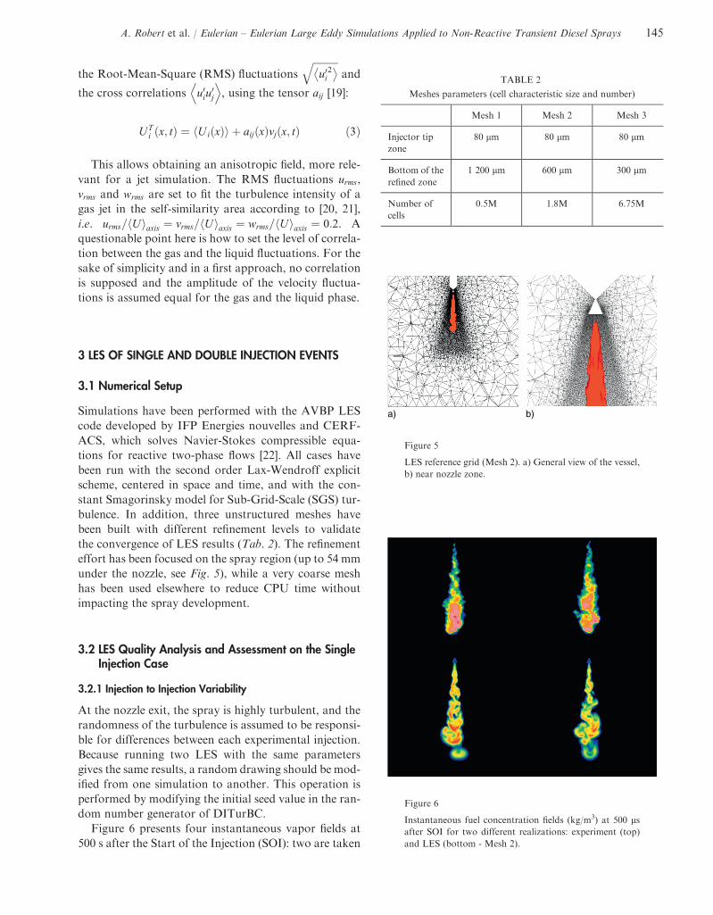
bulence. In addition, three unstructured meshes have

been built with different refinement levels to validate

the convergence of LES results (Tab. 2). The refinement

effort has been focused on the spray region (up to 54 mm

under the nozzle, see Fig. 5), while a very coarse mesh

has been used elsewhere to reduce CPU time without

impacting the spray development.

3.2 LES Quality Analysis and Assessment on the SingleInjection Case

3.2.1 Injection to Injection Variability

At the nozzle exit, the spray is highly turbulent, and the

randomness of the turbulence is assumed to be responsi-

ble for differences between each experimental injection.

Because running two LES with the same parameters

gives the same results, a random drawing should be mod-

ified from one simulation to another. This operation is

performed by modifying the initial seed value in the ran-

dom number generator of DITurBC.

Figure 6 presents four instantaneous vapor fields at

500 s after the Start of the Injection (SOI): two are taken

TABLE 2

Meshes parameters (cell characteristic size and number)

Mesh 1 Mesh 2 Mesh 3

Injector tip

zone

80 lm 80 lm 80 lm

Bottom of the

refined zone

1 200 lm 600 lm 300 lm

Number of

cells

0.5M 1.8M 6.75M

a) b)

Figure 5

LES reference grid (Mesh 2). a) General view of the vessel,

b) near nozzle zone.

Figure 6

Instantaneous fuel concentration fields (kg/m3) at 500 lsafter SOI for two different realizations: experiment (top)

and LES (bottom - Mesh 2).


from experiments (top) and two from LES (bottom)

obtained using Mesh 2. First of all, the simulated spray

structures look quite close to experimental ones, notably

the spray angle, penetration and large scale distortions

are correctly represented. In addition, comparing the

two LES realizations, this structure is clearly affected

by turbulence injection, which confirms the potential of

the turbulence injection method to mimic injection to

injection variability. Nevertheless, the qualitative agree-

ment between simulations and experiments is not per-

fect. Notably experimental vapor fields seem smoother

than numerical ones, especially because of the presence

of smaller structures inside the spray, and also due to

the filtering operation needed to reduce noise from the

raw experimental images. Moreover, a pocket of vapor

is present at the leading edge of the spray in the LES,

while being not observed experimentally. These differ-

ences will be discussed further in this paper.

It should also be noticed that the observed variability

seems high, indicating that a quite large number of real-

izations should be simulated to get a reasonable statisti-

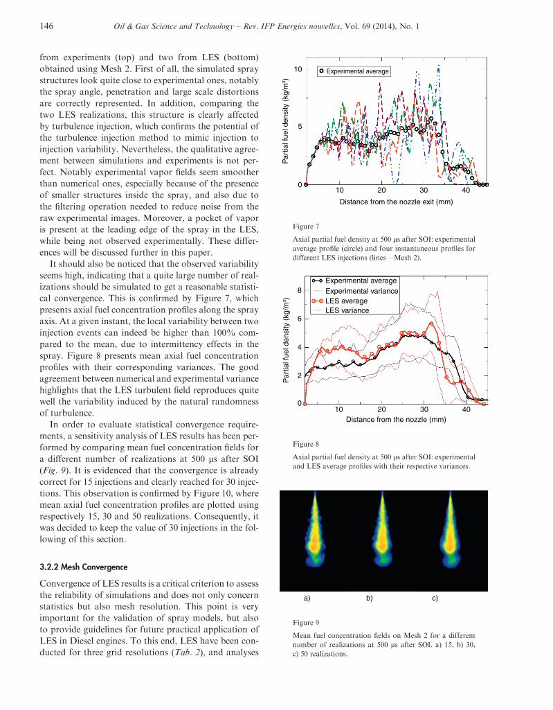
cal convergence. This is confirmed by Figure 7, which

presents axial fuel concentration profiles along the spray

axis. At a given instant, the local variability between two

injection events can indeed be higher than 100% com-

pared to the mean, due to intermittency effects in the

spray. Figure 8 presents mean axial fuel concentration

profiles with their corresponding variances. The good

agreement between numerical and experimental variance

highlights that the LES turbulent field reproduces quite

well the variability induced by the natural randomness

of turbulence.

In order to evaluate statistical convergence require-

ments, a sensitivity analysis of LES results has been per-

formed by comparing mean fuel concentration fields for

a different number of realizations at 500 ls after SOI

(Fig. 9). It is evidenced that the convergence is already

correct for 15 injections and clearly reached for 30 injec-

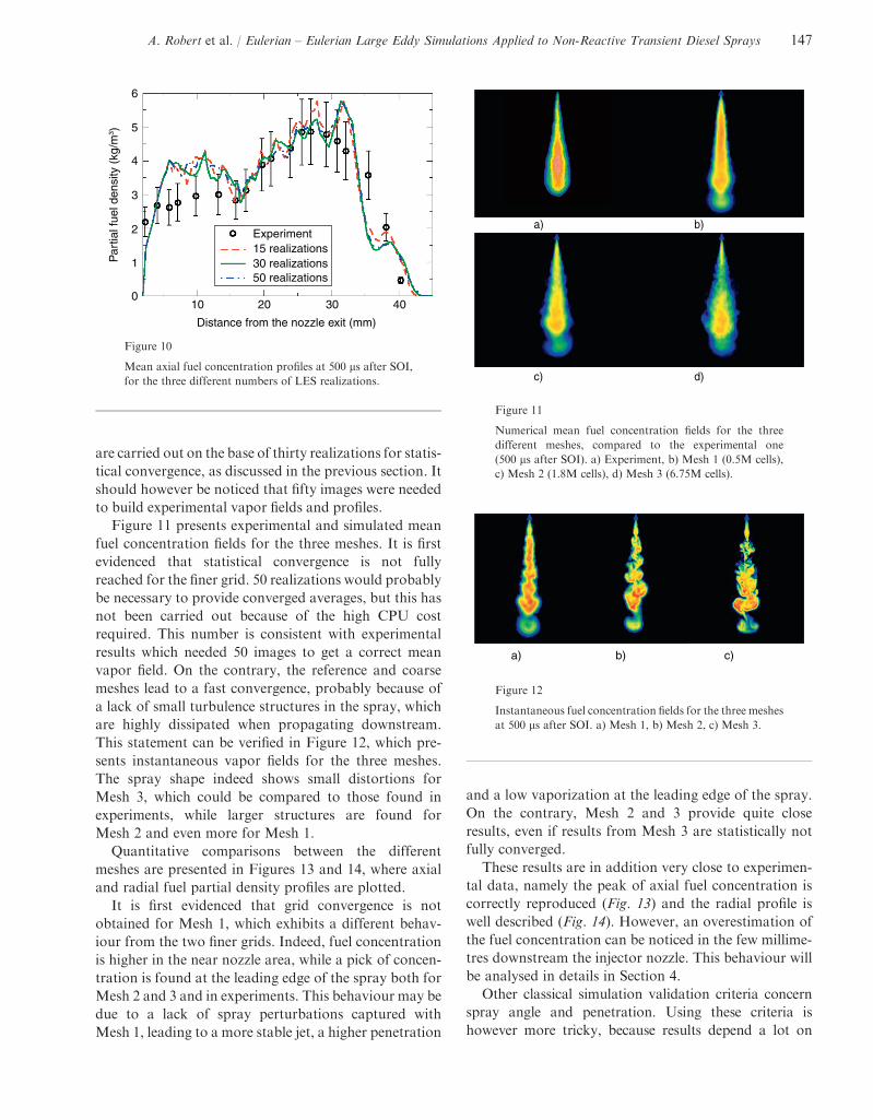
tions. This observation is confirmed by Figure 10, where

mean axial fuel concentration profiles are plotted using

respectively 15, 30 and 50 realizations. Consequently, it

was decided to keep the value of 30 injections in the fol-

lowing of this section.

3.2.2 Mesh Convergence

Convergence of LES results is a critical criterion to assess

the reliability of simulations and does not only concern

statistics but also mesh resolution. This point is very

important for the validation of spray models, but also

to provide guidelines for future practical application of

LES in Diesel engines. To this end, LES have been con-

ducted for three grid resolutions (Tab. 2), and analyses

10 20 30 40Distance from the nozzle (mm)

Par

tial f

uel d

ensi

ty (

kg/m

3 )8

6

4

2

0

Experimental averageExperimental varianceLES averageLES variance

Figure 8

Axial partial fuel density at 500 ls after SOI: experimental

and LES average profiles with their respective variances.

10

5

010 20 30 40

Distance from the nozzle exit (mm)

Par

tial f

uel d

ensi

ty (

kg/m

3 )

Experimental average

Figure 7

Axial partial fuel density at 500 ls after SOI: experimental

average profile (circle) and four instantaneous profiles for

different LES injections (lines – Mesh 2).

a) b) c)

Figure 9

Mean fuel concentration fields on Mesh 2 for a different

number of realizations at 500 ls after SOI. a) 15, b) 30,

c) 50 realizations.


are carried out on the base of thirty realizations for statis-

tical convergence, as discussed in the previous section. It

should however be noticed that fifty images were needed

to build experimental vapor fields and profiles.

Figure 11 presents experimental and simulated mean

fuel concentration fields for the three meshes. It is first

evidenced that statistical convergence is not fully

reached for the finer grid. 50 realizations would probably

be necessary to provide converged averages, but this has

not been carried out because of the high CPU cost

required. This number is consistent with experimental

results which needed 50 images to get a correct mean

vapor field. On the contrary, the reference and coarse

meshes lead to a fast convergence, probably because of

a lack of small turbulence structures in the spray, which

are highly dissipated when propagating downstream.

This statement can be verified in Figure 12, which pre-

sents instantaneous vapor fields for the three meshes.

The spray shape indeed shows small distortions for

Mesh 3, which could be compared to those found in

experiments, while larger structures are found for

Mesh 2 and even more for Mesh 1.

Quantitative comparisons between the different

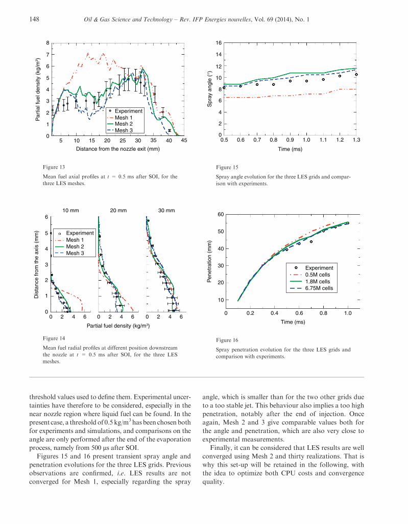
meshes are presented in Figures 13 and 14, where axial

and radial fuel partial density profiles are plotted.

It is first evidenced that grid convergence is not

obtained for Mesh 1, which exhibits a different behav-

iour from the two finer grids. Indeed, fuel concentration

is higher in the near nozzle area, while a pick of concen-

tration is found at the leading edge of the spray both for

Mesh 2 and 3 and in experiments. This behaviour may be

due to a lack of spray perturbations captured with

Mesh 1, leading to a more stable jet, a higher penetration

and a low vaporization at the leading edge of the spray.

On the contrary, Mesh 2 and 3 provide quite close

results, even if results from Mesh 3 are statistically not

fully converged.

These results are in addition very close to experimen-

tal data, namely the peak of axial fuel concentration is

correctly reproduced (Fig. 13) and the radial profile is

well described (Fig. 14). However, an overestimation of

the fuel concentration can be noticed in the few millime-

tres downstream the injector nozzle. This behaviour will

be analysed in details in Section 4.

Other classical simulation validation criteria concern

spray angle and penetration. Using these criteria is

however more tricky, because results depend a lot on

a) b) c)

Figure 12

Instantaneous fuel concentration fields for the three meshes

at 500 ls after SOI. a) Mesh 1, b) Mesh 2, c) Mesh 3.

a) b)

c) d)

Figure 11

Numerical mean fuel concentration fields for the three

different meshes, compared to the experimental one

(500 ls after SOI). a) Experiment, b) Mesh 1 (0.5M cells),

c) Mesh 2 (1.8M cells), d) Mesh 3 (6.75M cells).

10 20 30 40


Par

tial f

uel d

ensi

ty (

kg/m

3 )

4

5

6

2

0

1

Experiment

3

15 realizations30 realizations50 realizations

Figure 10

Mean axial fuel concentration profiles at 500 ls after SOI,

for the three different numbers of LES realizations.


threshold values used to define them. Experimental uncer-

tainties have therefore to be considered, especially in the

near nozzle region where liquid fuel can be found. In the

present case, a thresholdof 0.5 kg/m3has been chosenboth

for experiments and simulations, and comparisons on the

angle are only performed after the end of the evaporation

process, namely from 500 ls after SOI.

Figures 15 and 16 present transient spray angle and

penetration evolutions for the three LES grids. Previous

observations are confirmed, i.e. LES results are not

converged for Mesh 1, especially regarding the spray

angle, which is smaller than for the two other grids due

to a too stable jet. This behaviour also implies a too high

penetration, notably after the end of injection. Once

again, Mesh 2 and 3 give comparable values both for

the angle and penetration, which are also very close to

experimental measurements.

Finally, it can be considered that LES results are well

converged using Mesh 2 and thirty realizations. That is

why this set-up will be retained in the following, with

the idea to optimize both CPU costs and convergence

quality.

16

14

12

10

8

6

4

2

00.5 0.6 0.7 0.8 0.9 1.0 1.1 1.2 1.3

Time (ms)

Spr

ay a

ngle

(°)

Figure 15

Spray angle evolution for the three LES grids and compar-

ison with experiments.

60

50

40

30

20

10

0 0.2 0.4 0.6 0.8 1.0

Time (ms)

Pen

etra

tion

(mm

)

Experiment0.5M cells1.8M cells6.75M cells

Figure 16

Spray penetration evolution for the three LES grids and

comparison with experiments.

Dis

tanc

e fr

om th

e ax

is (

mm

)

Partial fuel density (kg/m3)

10 mm 20 mm 30 mm6

5

4

3

2

1

00 2 4 6 0 2 4 6 0 2 4 6

ExperimentMesh 1Mesh 2Mesh 3

Figure 14

Mean fuel radial profiles at different position downstream

the nozzle at t = 0.5 ms after SOI, for the three LES

meshes.

Par

tial f

uel d

ensi

ty (

kg/m

3 )8

6

7

4

5

2

3

05 10 15 20 25

Experiment

30

Mesh 1Mesh 2Mesh 3

35 40 45

1


Figure 13

Mean fuel axial profiles at t = 0.5 ms after SOI, for the

three LES meshes.


3.2.3 LES Quality Assessment

An important question regarding LES is to know if a suf-

ficient part of the turbulent flow energy is directly

resolved by the computational grid. In this case, it is con-

sidered that the biggest scales of the flow, which behav-

iour is difficult to model using a SGS model, are well

captured, then conferring a high level of confidence in

the LES predictivity. A convenient criterion to analyse

LES quality is based on the work of Pope [23]. Following

this approach, the ratio of the SGS flow energy over the

total turbulent energy is evaluated as:

Ksgs

Ktotal¼ Ksgs

Ksgs þ Kturbð4Þ

where the turbulent kinetic energy Kturb is given by:

Kturb ¼ 1

2u2rms þ v2rms þ w2

rms

� � ð5Þ

and urms, vrms and wrms are the components of the

root mean square velocity. The SGS kinetic energy

is obtained from the SGS turbulent viscosity ttfollowing:

Ksgs ¼ ttCkD

� �2

ð6Þ

with Ck ¼ 0:1 and D the local characteristic length scale

of the grid given by the cube root of the cell volume.

Finally, the Pope criterion is satisfied when the SGS

kinetic energy is less than 20% of the total turbulent

energy.

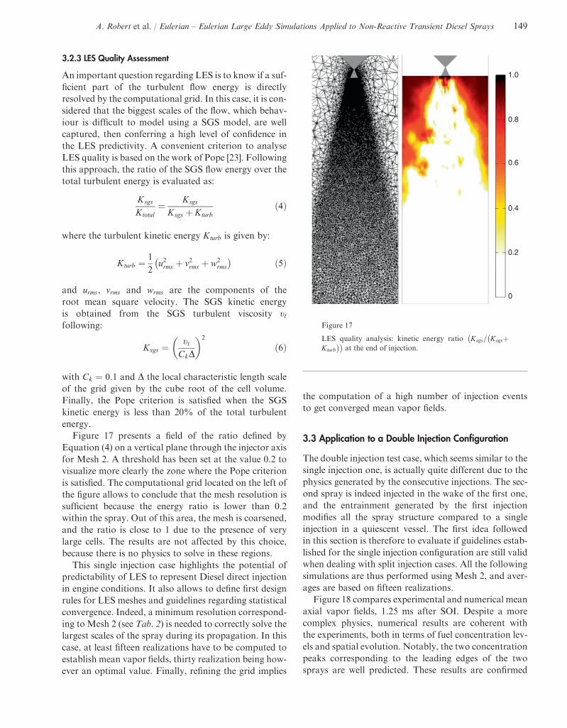
Figure 17 presents a field of the ratio defined by

Equation (4) on a vertical plane through the injector axis

for Mesh 2. A threshold has been set at the value 0.2 to

visualize more clearly the zone where the Pope criterion

is satisfied. The computational grid located on the left of

the figure allows to conclude that the mesh resolution is

sufficient because the energy ratio is lower than 0.2

within the spray. Out of this area, the mesh is coarsened,

and the ratio is close to 1 due to the presence of very

large cells. The results are not affected by this choice,

because there is no physics to solve in these regions.

This single injection case highlights the potential of

predictability of LES to represent Diesel direct injection

in engine conditions. It also allows to define first design

rules for LES meshes and guidelines regarding statistical

convergence. Indeed, a minimum resolution correspond-

ing to Mesh 2 (see Tab. 2) is needed to correctly solve the

largest scales of the spray during its propagation. In this

case, at least fifteen realizations have to be computed to

establish mean vapor fields, thirty realization being how-

ever an optimal value. Finally, refining the grid implies

the computation of a high number of injection events

to get converged mean vapor fields.

3.3 Application to a Double Injection Configuration

The double injection test case, which seems similar to the

single injection one, is actually quite different due to the

physics generated by the consecutive injections. The sec-

ond spray is indeed injected in the wake of the first one,

and the entrainment generated by the first injection

modifies all the spray structure compared to a single

injection in a quiescent vessel. The first idea followed

in this section is therefore to evaluate if guidelines estab-

lished for the single injection configuration are still valid

when dealing with split injection cases. All the following

simulations are thus performed using Mesh 2, and aver-

ages are based on fifteen realizations.

Figure 18 compares experimental and numerical mean

axial vapor fields, 1.25 ms after SOI. Despite a more

complex physics, numerical results are coherent with

the experiments, both in terms of fuel concentration lev-

els and spatial evolution. Notably, the two concentration

peaks corresponding to the leading edges of the two

sprays are well predicted. These results are confirmed

1.0

0.8

0.6

0.4

0.2

0

Figure 17

LES quality analysis: kinetic energy ratio Ksgs= Ksgsþ��

Kturb

��at the end of injection.


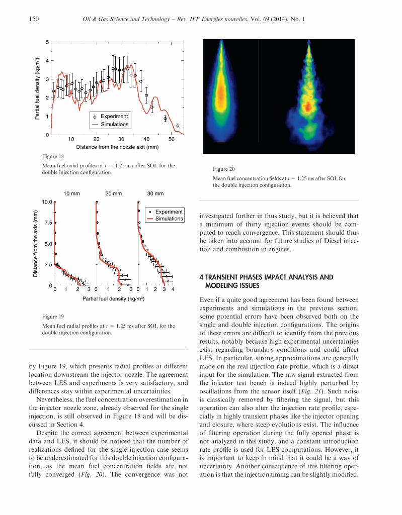
by Figure 19, which presents radial profiles at different

location downstream the injector nozzle. The agreement

between LES and experiments is very satisfactory, and

differences stay within experimental uncertainties.

Nevertheless, the fuel concentration overestimation in

the injector nozzle zone, already observed for the single

injection, is still observed in Figure 18 and will be dis-

cussed in Section 4.

Despite the correct agreement between experimental

data and LES, it should be noticed that the number of

realizations defined for the single injection case seems

to be underestimated for this double injection configura-

tion, as the mean fuel concentration fields are not

fully converged (Fig. 20). The convergence was not

investigated further in thus study, but it is believed that

a minimum of thirty injection events should be com-

puted to reach convergence. This statement should thus

be taken into account for future studies of Diesel injec-

tion and combustion in engines.

4 TRANSIENT PHASES IMPACT ANALYSIS ANDMODELING ISSUES

Even if a quite good agreement has been found between

experiments and simulations in the previous section,

some potential errors have been observed both on the

single and double injection configurations. The origins

of these errors are difficult to identify from the previous

results, notably because high experimental uncertainties

exist regarding boundary conditions and could affect

LES. In particular, strong approximations are generally

made on the real injection rate profile, which is a direct

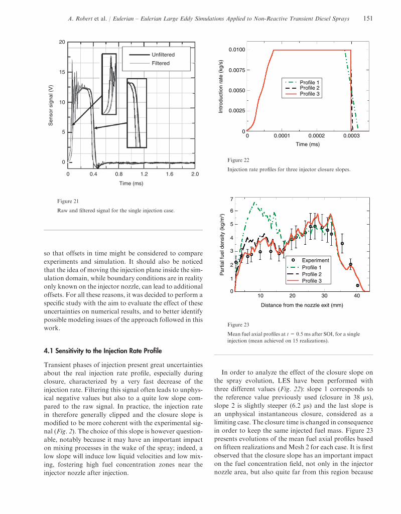
input for the simulation. The raw signal extracted from

the injector test bench is indeed highly perturbed by

oscillations from the sensor itself (Fig. 21). Such noise

is classically removed by filtering the signal, but this

operation can also alter the injection rate profile, espe-

cially in highly transient phases like the injector opening

and closure, where steep evolutions exist. The influence

of filtering operation during the fully opened phase is

not analyzed in this study, and a constant introduction

rate profile is used for LES computations. However, it

is important to keep in mind that it could be a way of

uncertainty. Another consequence of this filtering oper-

ation is that the injection timing can be slightly modified,

5

4

3

2

1

010 20 30 40 50


Par

tial f

uel d

ensi

ty (

kg/m

3 )

Experiment

Simulations

Figure 18

Mean fuel axial profiles at t = 1.25 ms after SOI, for the

double injection configuration.

Dis

tanc

e fr

om th

e ax

is (

mm

)

Partial fuel density (kg/m3)

0 00

10.0

7.5

5.0

2.5

01 1 13 3 32 2 2 4

10 mm 20 mm 30 mm

ExperimentSimulations

Figure 19

Mean fuel radial profiles at t = 1.25 ms after SOI, for the

double injection configuration.

Figure 20

Mean fuel concentration fields at t=1.25 ms after SOI, for

the double injection configuration.


so that offsets in time might be considered to compare

experiments and simulation. It should also be noticed

that the idea of moving the injection plane inside the sim-

ulation domain, while boundary conditions are in reality

only known on the injector nozzle, can lead to additional

offsets. For all these reasons, it was decided to perform a

specific study with the aim to evaluate the effect of these

uncertainties on numerical results, and to better identify

possible modeling issues of the approach followed in this

work.

4.1 Sensitivity to the Injection Rate Profile

Transient phases of injection present great uncertainties

about the real injection rate profile, especially during

closure, characterized by a very fast decrease of the

injection rate. Filtering this signal often leads to unphys-

ical negative values but also to a quite low slope com-

pared to the raw signal. In practice, the injection rate

in therefore generally clipped and the closure slope is

modified to be more coherent with the experimental sig-

nal (Fig. 2). The choice of this slope is however question-

able, notably because it may have an important impact

on mixing processes in the wake of the spray; indeed, a

low slope will induce low liquid velocities and low mix-

ing, fostering high fuel concentration zones near the

injector nozzle after injection.

In order to analyze the effect of the closure slope on

the spray evolution, LES have been performed with

three different values (Fig. 22): slope 1 corresponds to

the reference value previously used (closure in 38 ls),slope 2 is slightly steeper (6.2 ls) and the last slope is

an unphysical instantaneous closure, considered as a

limiting case. The closure time is changed in consequence

in order to keep the same injected fuel mass. Figure 23

presents evolutions of the mean fuel axial profiles based

on fifteen realizations andMesh 2 for each case. It is first

observed that the closure slope has an important impact

on the fuel concentration field, not only in the injector

nozzle area, but also quite far from this region because

20

15

10

5

0

0 0.4 0.8 1.2 1.6 2.0

Time (ms)

Sen

sor

sign

al (

V)

Unfiltered

Filtered

Figure 21

Raw and filtered signal for the single injection case.

0.0100

0.0075

0.0025

0.0050

00 0.0001 0.0002 0.0003

Time (ms)

Intr

oduc

tion

rate

(kg

/s)

Profile 1Profile 2Profile 3

Figure 22

Injection rate profiles for three injector closure slopes.


10 20 30 40

7

6

5

4

3

2

1

0

Par

tial f

uel d

ensi

ty (

kg/m

3 )

ExperimentProfile 1Profile 2Profile 3

Figure 23

Mean fuel axial profiles at t=0.5 ms after SOI, for a single

injection (mean achieved on 15 realizations).


of entrainment effects from the leading edge of the

spray. In addition, steep slopes, more coherent with

the raw experimental signal, allow to correctly match

experimental results in the near nozzle area. However,

the fact that slope 3 brings some improvements on the

fuel concentration profile compared to the reference

slope 1 should not be considered as a physical behaviour

because the injector closure is instantaneous. This point

will be discussed further in Section 4.3.

The same kind of study has been performed regarding

the opening slope with the aim to improve fuel concen-

tration profiles at the leading edge of the spray (not

shown). However, whatever the slope, the fuel pocket

observed in this region still exists. It was also observed

that this pocket is less pronounced when increasing the

mesh resolution and mainly appears when the spray

reaches low resolution zones. It is then believed that

this behaviour may not be linked to errors on the injec-

tion rate profile, but to excessive diffusion at the leading

edge of the spray leading to fuel accumulation in this

zone.

4.2 Impact of the Visualisation Timing

Uncertainties regarding injection boundary conditions

do not only concern profiles but also the real injection

timing. A first source of error is the response time of the

injector. For instance, for the single injection case, the

duration of the injector order is 500 ls whereas the realinjection time is about 300 ls. Other approximations

can be done on introduction rate measurements because

the sensor used also has a response time. The same obser-

vation can be done for the uncertainty of camera response

and exposure time which provides the images used to

obtain experimental fuel concentration profiles. Finally,

filtering the raw signal also alters this timing (Fig. 21).

However, comparing experimental and numerical fields

which do not have exactly the same timing can lead to

huge fictive errors. This is particularly important for com-

parisons performed at the injector closure because of the

very fast decrease of velocity [24]. In this case, an error of

several tenmicroseconds could have a great impact on the

fuel concentration field.

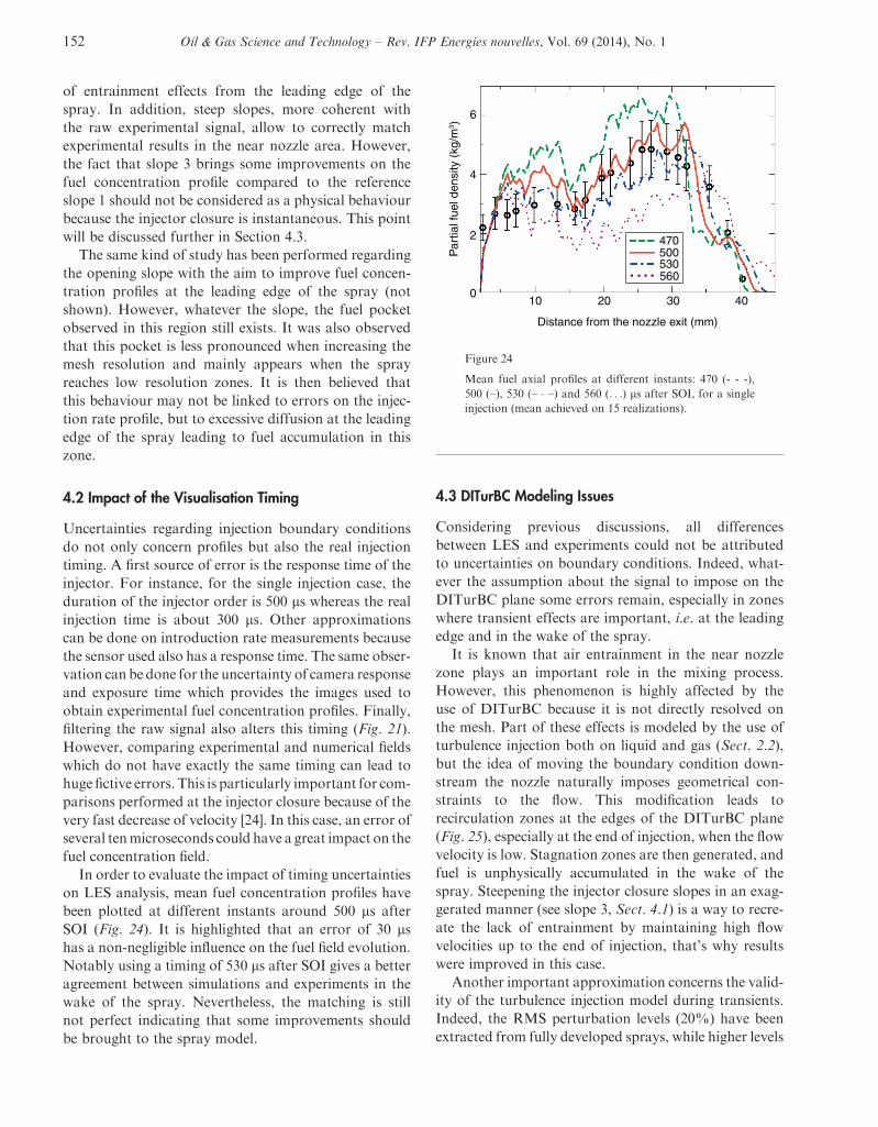
In order to evaluate the impact of timing uncertainties

on LES analysis, mean fuel concentration profiles have

been plotted at different instants around 500 ls after

SOI (Fig. 24). It is highlighted that an error of 30 lshas a non-negligible influence on the fuel field evolution.

Notably using a timing of 530 ls after SOI gives a better

agreement between simulations and experiments in the

wake of the spray. Nevertheless, the matching is still

not perfect indicating that some improvements should

be brought to the spray model.

4.3 DITurBC Modeling Issues

Considering previous discussions, all differences

between LES and experiments could not be attributed

to uncertainties on boundary conditions. Indeed, what-

ever the assumption about the signal to impose on the

DITurBC plane some errors remain, especially in zones

where transient effects are important, i.e. at the leading

edge and in the wake of the spray.

It is known that air entrainment in the near nozzle

zone plays an important role in the mixing process.

However, this phenomenon is highly affected by the

use of DITurBC because it is not directly resolved on

the mesh. Part of these effects is modeled by the use of

turbulence injection both on liquid and gas (Sect. 2.2),

but the idea of moving the boundary condition down-

stream the nozzle naturally imposes geometrical con-

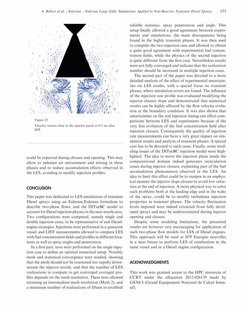
straints to the flow. This modification leads to

recirculation zones at the edges of the DITurBC plane

(Fig. 25), especially at the end of injection, when the flow

velocity is low. Stagnation zones are then generated, and

fuel is unphysically accumulated in the wake of the

spray. Steepening the injector closure slopes in an exag-

gerated manner (see slope 3, Sect. 4.1) is a way to recre-

ate the lack of entrainment by maintaining high flow

velocities up to the end of injection, that’s why results

were improved in this case.

Another important approximation concerns the valid-

ity of the turbulence injection model during transients.

Indeed, the RMS perturbation levels (20%) have been

extracted from fully developed sprays, while higher levels


Par

tial f

uel d

ensi

ty (

kg/m

3 )

6

4

2

010 20 30

470500530560

40

Figure 24

Mean fuel axial profiles at different instants: 470 (- - -),

500 (–), 530 (– � –) and 560 (. . .) ls after SOI, for a single

injection (mean achieved on 15 realizations).


could be expected during closure and opening. This may

allow to enhance air entrainment and mixing in these

phases and to reduce accumulation effects observed in

the LES, avoiding to modify injection profiles.

CONCLUSION

This paper was dedicated to LES simulations of transient

Diesel sprays using an Eulerian/Eulerian formalism to

describe two-phase flows, and the DITurBC model to

account forDiesel injection physics in the near nozzle area.

Two configurations were computed, namely single and

double injection cases, to be representative of real Diesel-

engine strategies. Injections were performed in a quiescent

vessel, and LIEF measurements allowed to compare LES

with fuel concentration fields and profiles in different loca-

tions as well as spray angles and penetration.

In a first part, tests were performed on the single injec-

tion case to define an optimal numerical setup. Notably

mesh and statistical convergence were studied, showing

that the mesh should not be coarsened too rapidly down-

stream the injector nozzle, and that the number of LES

realizations to compute to get converged averaged pro-

files depends on the mesh resolution. These tests allowed

retaining an intermediate mesh resolution (Mesh 2), and

a minimum number of realizations of fifteen to establish

reliable statistics, spray penetration and angle. This

setup finally allowed a good agreement between experi-

ments and simulations, the main discrepancies being

found in the highly transient phases. It was then used

to compute the two-injection case and allowed to obtain

a quite good agreement with experimental fuel concen-

tration fields, while the physics of the second injection

is quite different from the first case. Nevertheless results

were not fully converged and indicate that the realization

number should be increased in multiple injection cases.

The second part of the paper was devoted to a more

detailed analysis of the effect of experimental uncertain-

ties on LES results, with a special focus on transient

phases, where simulation errors are found. The influence

of the injection rate profile was evaluated modifying the

injector closure slope and demonstrated that numerical

results can be highly affected by the flow velocity evolu-

tion at the boundary condition. It was also shown that

uncertainties on the real injection timing can affect com-

parisons between LES and experiments because of the

very fast evolution of the fuel concentration field after

injection closure. Consequently the quality of injection

rate measurements can have a very great impact on sim-

ulation results and analysis of transient phases. A special

care has to be devoted to such cases. Finally, some mod-

eling issues of the DITurBC injection model were high-

lighted. The idea to move the injection plane inside the

computational domain indeed generates recirculation

zones during injector closure, explaining part of the fuel

accumulation phenomenon observed in the LES. An

idea to limit this effect could be to steepen in an unphys-

ical manner the injector slope closure to avoid low veloc-

ities at the end of injection. A more physical way to solve

such problems both at the leading edge and in the wake

of the spray, could be to modify turbulence injection

properties in transient phases. The velocity fluctuation

levels imposed were indeed extracted from fully devel-

oped sprays and may be underestimated during injector

opening and closure.

Despite some modeling limitations, the presented

results are however very encouraging for application of

such two-phase flow models for LES of Diesel engines.

This approach will be used at IFP Energies nouvelles

in a near future to perform LES of combustion in the

same vessel and in a Diesel engine configuration.

ACKNOWLEDGMENTS

This work was granted access to the HPC resources of

CCRT under the allocation 2012-026139 made by

GENCI (Grand Equipement National de Calcul Inten-

sif).

Figure 25

Velocity vectors close to the injector patch at 0.5 ms after

SOI.


REFERENCES

1 Richard S., Colin O., Vermorel O., Benkenida A.,Angelberger C., Veynante D. (2007) Towards large eddysimulation of combustion in spark ignition engines, Proc.Combust. Inst. 31, 2, 3059-3066.

2 Vermorel O., Richard S., Colin O., Angelberger C.,Benkenida A., Veynante D. (2009) Towards the under-standing of cyclic variability in a spark ignited engine usingmulti-cycle LES, Combust. Flame 156, 1525-1541.

3 Enaux B., Granet V., Vermorel O., Lacour C., Thobois L.,Dugue V., Poinsot T. (2011) Large Eddy Simulation of amotored single-cylinder piston engine: numerical strategiesand validation, Flow Turbul. Combust. 86, 2, 153-177.

4 Granet V., Vermorel O., Lacour C., Enaux B., Dugue V.,Poinsot T. (2012) Large-Eddy Simulation and experimentalstudy of cycle-to-cycle variations of stable and unstableoperating points in a spark ignition engine,Combust. Flame159, 1562-1575.

5 Lecocq G., Richard S., Michel J.-B., Vervisch L. (2011) Anew LES model coupling flame surface density and tabu-lated kinetics approaches to investigate knock and pre-ignition in piston engines, Proc. Combust. Inst. 33, 6, 1215-1226.

6 Martinez L., Benkenida A., Cuenot B. (2007) TowardsLarge Eddy Simulation of Diesel Fuel Spray Using anEulerian-Eulerian Approach, ILASS-Europe.

7 Vuorinen V., Hillamo H., Nuutinen M., Kaario O., LarmiM., Fuchs L. (2011) Effect of Droplet Size and Atomiza-tion on Spray Shape: A Priori Study Using Large-EddySimulation, Flow Turb. Combust. 86, 533-561.

8 Vuorinen V., Hillamo H., Nuutinen M., Kaario O.,Larmi M., Fuchs L. (2010) Large-Eddy Simulation ofDroplet Stokes Number Effects on Turbulent Spray Shape,Atomization Sprays, 20, 93-114.

9 Hori T., Senda J., Kuge T., Gen Fujimoto H. (2006) LargeEddy Simulation of Non-Evaporative and EvaporativeDiesel Spray in Constant Volume Vessel by Use ofKIVALES, SAE Paper 2006-01-3334.

10 Fujimoto H., Hori T., Senda J. (2009) Effect of BreakupModel on Diesel Spray Structure Simulated by Large EddySimulation, SAE Paper 2009-24-0024.

11 Vuorinen V., Larmi M. (2008) Large-Eddy Simulation onthe Effect of Droplet Size Distribution on Mixing of Pas-sive Scalar in a Spray, SAE Paper 2008-01-0933.

12 Simonin O. (1996) Combustion and turbulence in twophase flows. Lecture series 1996-02, Von Karman Instituteof Fluid Dynamics.

13 Fevrier P., Simonin O., Squires K.D. (2005) Partitioningof particle velocities in gas-solid turbulent flows into acontinuous field and a spatially uncorrelated random dis-tribution: Theoretical formalism and numerical study,J. Fluid Mech. 533, 1-46.

14 Martinez L., Vie A., Jay S., Benkenida A., Cuenot B. (2009)Large Eddy Simulation of Fuel sprays using the EulerianMesoscopic Approach. Validations in realistic engine con-ditions, 11th ICLASS International Conference on LiquidAtomization and Sprays Systems, Vail, Colorado, USA.

15 Martinez L., Benkenida A., Cuenot B. (2010) A model forthe injection boundary conditions in the context of 3D sim-ulation of Diesel Spray: Methodology and validation, Fuel89, 1, 219-228.

16 Bruneaux G., Maligne D. (2009) Study of the Mixing andCombustion Processes of Consecutive Short Double Dieselinjections, SAE Paper 2009-01-1352.

17 Kraichan R. (1970) Diffusion by a Random Velocity Field,Phys. Fluids 13, 22-31.

18 SmirnovA., Shi S.,Celik I. (2000)RandomFlowSimulationswith bubble dynamics model, Proceedings of FEDSM00,ASME 2000 Fluids Engineering Division Summer Meeting,Vol. FEDSM2000-11215, Boston, Massachusetts, USA.

19 Klein M., Sadiki A., Janicka J. (2003) A digital filter-basedgeneration of inflow data for spatially developing numeri-cal simulation or large eddy simulation, J. Comput. Phys.186, 652-665.

20 Hussein H., Capp S., Georges W. (1994) velocity measure-ments in a high-reynolds-number-momentum-conserva-tive, axisymmetric turbulent jet, J. Fluid Mech. 258, 31-75.

21 Chaves H., Kirmse C., Obermeier F. (2004) Velocity mea-surements of dense Diesel fuel sprays in dense airization,Atomization Sprays 14, 589-609.

22 Moureau V., Lartigue G., Sommerer Y., Angelberger C.,Colin O., Poinsot T. (2005) Numerical methods forunsteady compressible multi-component reacting flows onfixed and moving grids, J. Comput. Phys. 2020, 2, 710-736.

23 Pope S.B. (2004) Ten questions concerning the large-eddysimulation of turbulent flows, New J. Phys. 6, 35.

24 Musculus M., Picket l. (2009) Entrainment waves in Dieseljets, SAE Paper 2009-01-1335.

Manuscript accepted in April 2013

Published online in November 2013

Copyright � 2013 IFP Energies nouvelles

Permission to make digital or hard copies of part or all of this work for personal or classroom use is granted without fee provided that copies are notmade or distributed for profit or commercial advantage and that copies bear this notice and the full citation on the first page. Copyrights forcomponents of this work owned by others than IFP Energies nouvelles must be honored. Abstracting with credit is permitted. To copy otherwise,to republish, to post on servers, or to redistribute to lists, requires prior specific permission and/or a fee: Request permission from InformationMission, IFP Energies nouvelles, fax. +33 1 47 52 70 96, or [email protected].


Documents

Eulerian â€” Eulerian Large Eddy Simulations Applied to Non