This Provisional PDF corresponds to the article as it appeared upon acceptance. Fully formattedPDF and full text (HTML) versions will be made available soon.

Performance of MIMO systems in measured indoor channels with transmitternoise

EURASIP Journal on Wireless Communications and Networking 2012,2012:109 doi:10.1186/1687-1499-2012-109

Paula M Castro (pcastro@udc.es)Jose P Gonzalez-Coma (jose.gcoma@udc.es)

Jose A Garcia-Naya (jagarcia@udc.es)Luis Castedo (luis@udc.es)

ISSN 1687-1499

Article type Research

Submission date 20 July 2011

Acceptance date 15 March 2012

Publication date 15 March 2012

Article URL http://jwcn.eurasipjournals.com/content/2012/1/109

This peer-reviewed article was published immediately upon acceptance. It can be downloaded,printed and distributed freely for any purposes (see copyright notice below).

For information about publishing your research in EURASIP WCN go to

http://jwcn.eurasipjournals.com/authors/instructions/

For information about other SpringerOpen publications go to

http://www.springeropen.com

EURASIP Journal on WirelessCommunications andNetworking

© 2012 Castro et al. ; licensee Springer.This is an open access article distributed under the terms of the Creative Commons Attribution License (http://creativecommons.org/licenses/by/2.0),

which permits unrestricted use, distribution, and reproduction in any medium, provided the original work is properly cited.

Performance of MIMO systems in measured

indoor channels with transmitter noise

Paula M Castro, Jose P Gonzalez-Coma, Jose A Garcıa-Naya∗ and Luis Castedo

Department of Electronics and Systems, University of A Coruna, Facultad de Informatica,

Campus de Elvina s/n, A Coruna 15071, Spain

∗Corresponding author: jagarcia@udc.es

Email addresses:

PMC: pcastro@udc.es

JPG-C: jose.gcoma@udc.es

LC: luis@udc.es

Abstract

This study analyzes the impact of transmitter noise on the performance of multiple-input multiple-output

(MIMO) systems with linear and nonlinear receivers and precoders. We show that the performance of

MIMO linear and decision-feedback receivers is not significantly influenced by the presence of transmitter

noise, which does not hold true in the case of MIMO systems with precoding. Nevertheless, we also

1

show that this degradation can be greatly alleviated when the transmitter noise is considered in the

MIMO precoder design. A MIMO testbed developed at the University of A Coruna has been employed

for experimentally evaluating how much the transmitter noise impacts the system performance. Both

the transmitter noise and the receiver noise covariance matrices have been estimated from a set of 260

indoor MIMO channel realizations. The impact of transmitter noise has been assessed in this realistic

scenario.

1 Introduction

Practical implementations of wireless transmitters suffer from a large number of impair-

ments such as quantization noise, sampling offset, phase noise, I/Q imbalance . . . which

can be classified into systematic and non-systematic effects. These impairments are nor-

mally ignored when multiple-input multiple-output (MIMO) signaling methods are designed.

However, noise generated at the transmitter can significantly affect predicted performance

in practical scenarios. For instance, the performance of a linear zero-forcing (ZF) MIMO

detector affected by the transmitter impairments of a MIMO orthogonal frequency-division

multiplexing (OFDM) hardware demonstrator is tested in [1], where it is shown how the per-

formance achieved by such noisy systems suffers from a loss greater than 4 dB for a bit error

rate (BER) of 10−2. More specifically, the impact of residual transmitter radio-frequency

(RF) impairments on both MIMO channel capacity and receiver performance is analyzed

in [2]. It has been demonstrated that maximum-likelihood (ML) and Max-log a posteriori

probability (APP) MIMO detection suffer from a substantial performance loss under the

presence of weak transmitter noise, whereas linear ZF receivers are much less affected.

In this study, the impact of residual non-deterministic, non-systematic transmit impair-

ments on MIMO signaling methods not considered in [1, 2] is studied. First of all, we focus

2

on MIMO systems with either linear receivers [3–5] or linear precoders [4–8]. We will also

focus on MIMO systems with nonlinear decision feedback (DF) receivers [9,10] and nonlinear

Tomlinson-Harashima (TH) precoders [5, 11, 12]. Both DF receivers and TH precoders are

widely used because of their good trade-off between performance and complexity. The mod-

ulo operator at the receiver of a MIMO system with TH precoding has also motivated the

proposal of a more general MIMO precoding technique where the data signal superimposed

with a perturbation signal inputs a linear filter at the transmitter. This scheme is referred to

as vector precoding (VP) in the literature [5,13]. The optimum perturbation signal is found

with a closest point search in a lattice. Despite its larger complexity, VP outperforms TH

precoding.

Although the impact of transmitter noise has been evaluated over spatially-white

Rayleigh channels in [14, 15] and some preliminary results obtained from testbed measure-

ments in an indoor scenario have been presented in [15, 16], only our study evaluates the

performance of all the aforementioned schemes affected by transmitter noise over measured

indoor channels by means of the testbed developed by the University of A Coruna [17].

Contrary to previous studies, not only the channel coefficients are measured using such a

testbed, but also a estimate of all the noise covariance matrices existing in practical MIMO

systems and of the signal-to-transmitter noise ratio (STxNR) are obtained and plugged into

the robust filter expressions to guarantee a complete reproducibility of a real indoor envi-

ronment and the evaluation in terms of BER performance of the proposed schemes under

such realistic conditions.

In this study, we show that noise generated at the transmitter significantly affects the

performance of MIMO systems with precoding. On the other hand, the performance of

both linear and DF MIMO receivers is more robust against the presence of transmitter

noise (cf. findings in the FP6-IST project MASCOT on multiuser MIMO communication

systems [18]). At a first glance, it seems natural that MIMO systems with precoding be

more sensitive to transmitter noise since channel equalization is carried out by processing

signals prior transmission. However, it will be also shown that the performance of precoded

MIMO systems can be substantially improved if the transmitter noise is considered inside

the precoder design.

3

This study is organized as follows. Section 2 introduces the MIMO signal model which

takes into account the aforementioned transmit RF impairments. The design of MIMO

linear receivers and precoders considering the presence of transmitter noise is addressed in

Section 3, whereas Section 4 focuses on MIMO nonlinear receivers (decision feedback) and

precoders (Tomlinson-Harashima and vector precoding). Section 5 briefly introduces the

MIMO testbed used to obtain measurements of the noise and of the channel parameters

necessary to reproduce a realistic, indoor scenario. Next, the performance of the MIMO sys-

tems analyzed in the previous sections is evaluated for this indoor scenario. Some concluding

remarks are presented in Section 6. Finally, Appendix 1 details all derivations corresponding

to the expressions of all linear and nonlinear filters derived including transmitter noise in

the optimizations.

Vectors and matrices are denoted by lower-case bold, and capital-bold letters, respec-

tively. We use E[•], tr(•), (•)T, (•)H, and ∥ • ∥2 for expectation, trace of a matrix, trans-

position, conjugate transposition, and Euclidean norm, respectively. The ith element of a

vector v is denoted by vi.

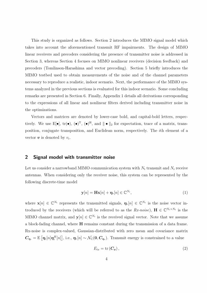
2 Signal model with transmitter noise

Let us consider a narrowband MIMO communication system with Nt transmit and Nr receive

antennas. When considering only the receiver noise, this system can be represented by the

following discrete-time model

y[n] = Hx[n] + ηr[n] ∈ CNr , (1)

where x[n] ∈ CNt represents the transmitted signals, ηr[n] ∈ CNr is the noise vector in-

troduced by the receivers (which will be referred to as the Rx-noise), H ∈ CNr×Nt is the

MIMO channel matrix, and y[n] ∈ CNr is the received signal vector. Note that we assume

a block-fading channel, where H remains constant during the transmission of a data frame.

Rx-noise is complex-valued, Gaussian-distributed with zero mean and covariance matrix

Cηr = E[ηr[n]η

Hr [n]

], i.e., ηr[n] ∼ NC(0,Cηr). Transmit energy is constrained to a value

Etx = tr (Cx) , (2)

4

where Cx is the covariance matrix corresponding to the input symbols x[n]. Accordingly,

we define the signal-to-receiver-noise ratio (SRxNR) as

SRxNR =EtxNr

tr(Cηr), (3)

where we have assumed that the channel is normalized to have a mean Frobenius norm equal

to Nt Nr.

When the residual impairments at the transmitter are taken into account, a more accurate

model for the transmitted signal is

xt[n] = x[n] + ηt[n] ∈ CNt , (4)

where ηt[n] ∈ CNt will be denoted as the Tx-noise. The subscript t will be used hereafter

to denote signals affected by Tx-noise. This noise encompasses different practical effects,

for example phase-noise. As explained in [2], Tx-noise is adequately modeled as an additive

Gaussian noise since it results from the sum of a large number of residual transmit impair-

ments. Tx-noise is assumed to be zero-mean with covariance matrix Cηt and the STxNR is

defined as

STxNR =Etx

tr(Cηt), (5)

where Etx is fixed and given by Equation (2). As an example, practical implementations

of the IEEE 802.11 (WiFi) standard achieve STxNR values ranging from 22 dB to 32 dB

(see [2] and references therein). The Tx-noise is also assumed to be statistically independent

from the Rx-noise. Note that we use the STxNR instead of the transmitter error vector

magnitude (EVM), which is another measure of the signal modulation quality (see [19]) that

additionally considers systematic errors.

Equations (1) and (4) are also adequate to represent a multi-antenna, multiuser wireless

system where a base station equipped with N antennas communicates with K single-antenna

users. When considering the uplink, Nt = K and Nr = N , whereas Nt = N and Nr = K for

the downlink. Although the channel model is the same, multiuser systems impose certain

constraints on the signal processing that can be carried out to recover the transmitted

information [20]. Indeed, for the uplink, the base station collects the signals from all the

users, so that they can be separated using conventional MIMO receiver methods. These

5

methods, however, cannot be used for the downlink since users do not normally cooperate

among them and, consequently, each receiver does not know the signals from the other

receivers. Therefore, in such a case signal separation can only be carried out by resorting to

precoding or to any other form of transmit processing.

3 MIMO linear receivers and precoders

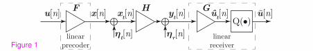
Figure 1 shows the block diagram of a general MIMO system with linear transmit and

receive processing. Notice that transmitter noise has been also included. We assume the

transmitter sends a set of Nr data streams encoded into the vector of transmitted symbols

u[n] ∈ ANr where A represents the utilized modulation alphabet. For linear transmit and

receive processing, one transmit filter, F ∈ CNt×Nr , so-called precoding filter, and one receive

filter, G ∈ CNr×Nr , are used to recover the transmitted data. Thus, after linear precoding,

the transmitted signal is

xt[n] = Fu[n] + ηt[n] ∈ CNt , (6)

and at the other end, the signal at the output of the receive filter G is given by

ut[n] = GHxt[n] +Gηr[n] ∈ CNr . (7)

This signal is the input to a symbol detector (represented by Q(•) in Figure 1) that maps

ut[n] onto the modulation alphabet A and produces the estimates of the transmitted symbols,

u[n].

3.1 MIMO linear receiver design with transmitter noise

Let us consider a simplified MIMO linear transmission system where the transmit filter is a

weighted identity matrix, i.e., F = pI. Thus, all the effort to compensate for the channel

spatial inter-symbol interference (ISI) is carried out by the receiver filter G (see [3, 5, 21]).

Elaborating on the signal model, the symbols at the output of the receiver filter can be

written as

ut[n] = u[n] +GHηt[n] ∈ CNt , (8)

6

where u[n] = pGHu[n] +Gηr[n] would be the received signal if there were no Tx-noise.

Next, let us define the error vector ϵt[n] = u[n] − ut[n]. The optimum receive filter G

and transmit weight p will be those that minimize the mean square error (MSE) E[||ϵt[n]||22]which, under the presence of Tx-noise, can be expressed as follows [3]

E[∥ϵt[n]∥22

]= E

[∥ϵ[n]∥22

]+ tr

(GHCηtH

HGH). (9)

Notice that E[∥ϵ[n]∥22

]is the cost function to be minimized in conventional minimum mean

square error (MMSE) linear receiver design where the transmitter noise is not accounted

for.

Similarly to the study in [5], it can be demonstrated that by restricting p ∈ R+ and

having in mind the transmit-energy constraint Etx = tr (Cx), the minimization of the cost

function given by Equation (9) produces the MMSE solution for the linear receiver given by

GMMSE =

(C−1

u

pMMSE

+ pMMSEHH(Cηr +HCηtH

H)−1

H

)−1

HH(Cηr +HCηtH

H)−1

,

pMMSE =

√Etx

tr (Cu),

(10)

where Cu is the covariance matrix of the transmitted symbols u[n].

From the MMSE design of the MIMO linear receiver, it is straightforward to obtain

the expressions for the ZF MIMO linear receiver [5]: it is the limiting case when tr(Cηr +

HCηtHH)/Etx → 0, i.e.,

GZF =(pZFH

H(Cηr +HCηtH

H)−1

H)−1

HH(Cηr +HCηtH

H)−1

,

pZF =

√Etx

tr (Cu). (11)

Note that a necessary condition for the existence of the filter GZF is that Nt ≤ Nr since it

exists only if HH(Cηr +HCηtHH)−1H is invertible.

3.2 MIMO linear precoder design with transmitter noise

Let us consider the MIMO transmission scheme dual to the previous one: the transmitted

symbols u[n] ∈ CNr are linearly precoded with the transmit filter F ∈ CNt×Nr and the receive

7

filter is a weighted identity matrix G = gI, where g ∈ R+. Thus, the transmitted signal is

xt[n] = Fu[n] + ηt[n] ∈ CNt , (12)

and the signal at the receiver input is given by

yt[n] = y[n] +Hηt[n] ∈ CNr , (13)

where y[n] = HFu[n] + ηr[n] would be the received signal if there were no Tx-noise. After

multiplication by the receive gain, g, we get the estimated symbols

ut[n] = u[n] + gHηt[n] ∈ CNr , (14)

where u[n] = gy[n]. We restrict the scalar value g to being common to all the receivers to

simplify the optimization procedure.

The optimum transmit and receive filters are those that minimize the MSE between u[n]

and ut[n] subject to the transmit-energy constraint Etx = tr (Cx) (see [3, 5–7]). Again, let

us define the error vector ϵt[n] = u[n]− ut[n] and express the MSE cost function as

E[∥ϵt[n]∥22

]= E

[∥ϵ[n]∥22

]+ tr

(|g|2HCηtH

H), (15)

where E[||ϵ[n]||22] is the MSE when there is no Tx-noise [4, 5, 8].

Minimizing this cost function produces the MMSE solution for the MIMO linear precod-

ing filter given by

FMMSE = g−1MMSE

(HHH + ξtI

)−1HH,

gMMSE =

√tr((HHH + ξtI)

−2 HHCuH)

Etx

,

(16)

where ξt = ξ + tr(HCηtHH)/Etx, with ξ being the inverse of the SRxNR defined in Equa-

tion (5).

By applying the matrix inversion lemma to the MMSE solution of Equation (16) and

considering afterwards the limiting case when ξt → 0, the expressions for the ZF linear

precoder can be readily obtained and expressed as follows

FZF = g−1ZFH

H(HHH)−1,

gZF =

√tr((HHH)−1 Cu

)Etx

. (17)

8

4 MIMO nonlinear receivers and precoders

In this section, we focus on MIMO systems that use either nonlinear transmitters or non-

linear receivers to recover the transmitted data. It is well known that maximum likelihood

detection (MLD) is the optimum detection scheme in the sense of minimizing the probabil-

ity of a symbol being erroneously detected. The computational complexity of MLD grows

exponentially with the number of transmit antennas and the modulation alphabet size and,

for this reason, suboptimum nonlinear detection schemes such as the decision feedback one

are preferred in a large number of practical situations.

However, decision-feedback receivers suffer from the major drawback of error propagation

caused by feeding back erroneous decisions. One way to avoid this harmful effect is to perform

a nonlinear filtering similar to that in DF but at the transmitter side. This idea leads to the

concept of Tomlinson-Harashima precoding (THP). Finally, VP is another form of nonlinear

MIMO transmit processing which will be considered in this section. Similarly to MLD, VP

consists in a lattice search carried out at the transmitter instead of at the receiver side.

The impact of transmitter noise on the performance of MLD has already been analyzed

in [2]. In the following sections, we will derive the expressions of the filters for the remaining

nonlinear transceivers when the Tx-noise is accounted for.

4.1 MIMO decision feedback receiver design with transmitter noise

Figure 2 plots the block diagram of a MIMO system with a DF receiver. Information symbols

will be represented by u[n] ∈ ANt , where A denotes the modulation alphabet, which are

directly sent by the transmit antennas. It is assumed that u[n] is zero mean with covariance

matrix denoted by Cu.

It is apparent from Equations (1) and (4) that the input signal at the receiver can be

written as

yt[n] = y[n] +Hηt[n] ∈ CNr , (18)

where y[n] = Hu[n] + ηr[n] is the received signal if there is no Tx-noise [5].

In DF reception, the signals at the channel output are passed through the feedforward

filter G ∈ CNt×Nr , which forces the ISI to be spatially causal and the error to be spatially

9

white (i.e., minimum variance). By means of the feedback filter I − B ∈ CNt×Nt and of

the feedback loop shown in Figure 2, ISI can be recursively canceled without changing the

statistical properties of the noise provided that the noise variance is sufficiently small so that

the symbol detector (represented by Q(•) in Figure 2) produces correctly detected symbols.

By elaborating on the signal model according to Figure 2, the estimated signal ut[n] can be

written as

ut[n] = Gyt[n] + (I −B) u[n], (19)

where yt[n] is defined as in Equation (18) and u[n] ∈ ANt denotes the detected symbols after

the threshold quantizer.

The order in which symbols are detected has a significant influence on the performance

of DF MIMO receivers. In the system model shown in Figure 2, the ordering is obtained

with the multiplication of the detected symbols, u[n], by the permutation matrix P T. This

multiplication produces up[n], which constitutes the vector of detected symbols conveniently

sorted. Having in mind that PP T = I, we have that u[n] = Pup[n] and hence, ut[n] can

be rewritten as

ut[n] = Gyt[n] + (I −B)P up[n].

The MMSE design of the DF MIMO receiver searches for the filtering and permutation

matrices that minimize the variance of the error vector

ϵt,p[n] = Pu[n]− ut[n].

Assuming correct decisions (i.e., up[n] = u[n]) and according to Equation (18), this error

vector can be rewritten as

ϵt,p[n] = BPu[n]−Gyt[n] = ϵp[n]−GHηt[n],

where ϵp[n] = BPu[n]−Gy[n] is the error vector when there is no Tx-noise. Since the Tx-

noise is independent from the Rx-noise and the transmitted signals, the MSE cost function

to be minimized can be written as

E[∥ϵt,p[n]∥22] = E[∥ϵp[n]∥22] + tr(GHCηtH

HGH), (20)

10

where E[∥ϵp[n]∥22] is the MSE with no Tx-noise. Notice that E[∥ϵp[n]∥22] is the cost func-

tion that is minimized in the conventional MMSE design, whereas the additional term

tr(GHCηtH

HGH)is the MSE improvement caused by the inclusion of the Tx-noise.

An MMSE design of the MIMO link that accounts for the Tx-noise should minimize the

MSE given by Equation (20). Similarly to the scenario without Tx-noise [22], minimization

of Equation (20) is readily accomplished from the Cholesky factorization with symmetric

permutation of

Φt = (HH(HCηtHH +Cηr)

−1H +C−1u )−1.

This factorization is given by PΦtPT = LDLH, where L is a unit lower triangular matrix

and D is a diagonal matrix. After this decomposition, it can be demonstrated that the

filters G and B for the MMSE DF nonlinear MIMO receiver solution are

GDFMMSE = DLHPHH(HCηtH

H +Cηr)−1,

BDFMMSE = L−1.

(21)

The minimum value of the MSE cost function is obtained plugging GDFMMSE and BDF

MMSE into

Equation (20). Hence, the MMSE value is

MMSEt,DF = tr (D) , (22)

where D is the diagonal matrix obtained from the Cholesky factorization with symmetric

permutation of Φt.

Notice that the MMSE expression given by Equation (22) depends on the permutation

matrix P . Brute force optimization of P can be carried out by computing the MMSE for

all the Nt! possible permutation matrices and choosing the one that provides the minimum

value of Equation (22). Alternatively, more efficient ordering algorithms (such as the one

described in [22]) can be used.

From the MMSE design of the DF receiver, it is straightforward to obtain the expressions

for the ZF DF receiver: it is the limiting case when tr(HCηtHH +Cηr)/Etx → 0. The final

expressions for the ZF DF filters are exactly the same as before although L and D should

be obtained from the Cholesky decomposition of

Φt = (HH(HCηtHH +Cηr)

−1H)−1.

11

4.2 MIMO Tomlinson-Harashima precoder design with transmitter noise

Figure 3 shows the block diagram of a MIMO system employing THP. THP is a nonlinear

precoding technique made up of a feedforward filter F ∈ CNt×Nr , a feedbackward filter I −B ∈ CNr×Nr , and a modulo operator, represented in Figure 3 by M(•). The modulo operator

is introduced to avoid the increase in transmit power due to the feedback loop [11]. Data

symbols sent from the transmitter will be represented by u[n] ∈ ANr , where A denotes the

modulation alphabet. The ordering considerably affects the performance of THP and, for this

reason, transmit symbols are passed through a permutation filter P . Minimization is carried

out under the restriction of B being a spatially causal filter and Etx being the transmitted

energy, i.e., E[∥x[n]∥22] = Etx, where x[n] = Fv[n] ∈ CNt is the transmitted signal, with

v[n] representing the output of the modulo operator. At reception, we assume that all the

receive antennas apply the same positive real value denoted by g. These assumptions are

necessary in order to arrive at closed-form, unique solutions for the MMSE THP design.

In order to carry out the THP optimization, and taking into account the linear represen-

tation of THP [5,11], the desired signal is denoted by d[n] and it is expressed as

d[n] = P TBv[n]. (23)

The received signal under the presence of Tx-noise is rewritten as

dt[n] = d[n] + gHηt[n] ∈ CNr , (24)

where d[n] = gHFv[n] + gηr[n] is the received signal when there is no Tx-noise. At the

receivers, the modulo operator is applied again to invert the effect of this operator at the

transmitter and the resulting signal is passed through a symbol detector (represented by

Q(•) in Figure 3) to produce the detected symbols u[n] ∈ ANr .

As explained in [5], the MMSE THP design searches for the filtering and permutation

matrices that minimize the variance of the error vector

ϵt[n] = P TBv[n]− dt[n] = ϵ[n]− gHηt[n],

where ϵ[n] = P TBv[n]− gy[n] is the error vector when there is no Tx-noise.

Since the Tx-noise is independent from the transmitted signal and the Rx-noise, the MSE

can be decomposed as

E[||ϵt[n]||22] = E[||ϵ[n]||22] + |g|2 tr(HCηtHH), (25)

12

where E[||ϵ[n]||22] is the MSE when there is no Tx-noise, which constitutes the cost function

that is minimized in the conventional MMSE design of THP.

Following similar derivations as in [12], the minimization of the MSE cost function in

Equation (25), subject to the mentioned constraints, can be carried out from the factorization

of

Φt = (HHH + ξtI)−1,

where

ξt = ξ + tr(HCηtHH)/Etx, (26)

with ξ = tr(Cηr)/Etx. The symmetrically permuted Cholesky decomposition of this matrix

is

PΦtPT = LHDL, (27)

where L and D are, respectively, unit lower triangular and diagonal matrices. Finally, the

MMSE solution for the THP filters that account for the Tx-noise is given by

F THPMMSE = gTHP,−1

MMSE HHP TLHD,

BTHPMMSE = L−1

(28)

The receive scalar weight gTHPMMSE is directly obtained from the transmit-energy constraint.

Assuming that it is real and positive, it is obtained that

gTHPMMSE =

√tr (HHP TLHD2CvLPH)

Etx

, (29)

where Cv is the covariance matrix of v[n], which is diagonal with entries depending on the

modulation alphabet [11].

The minimum value for the MSE cost function given by Equation (25) can be obtained

by substituting the expressions obtained for the optimum filters F THPMMSE and BTHP

MMSE, and

for the gain factor gTHPMMSE. It is easy to show that the final MMSE under the presence of

Tx-noise is

MMSEt,THP = ξt tr (CvD) , (30)

where ξt is given by Equation (26) and D is the diagonal matrix that results from the

permuted Cholesky factorization of Equation (27).

13

As it is done in [12], instead of testing all the possible permutation matrices to find the

one that minimizes the cost function of Equation (30), the ordering optimization can be

included in the computation of the Cholesky decomposition of Equation (27).

Again, it is straightforward to obtain the expressions for the ZF THP design as the

limiting case when ξt → 0. The expressions for the filters F THPZF and BTHP

ZF are equal to those

obtained for F THPMMSE and BTHP

MMSE, respectively, although the matrices P , L, and D should

be obtained from the symmetrically permuted Cholesky factorization of

Φt = (HHH)−1.

4.3 MIMO vector precoder design with transmitter noise

Figure 4 shows the block diagram of a MIMO system with VP. The transmitter has the

freedom to add an arbitrary perturbation signal a[n] ∈ τZNr + j τZNr to the data signal

prior to the linear transformation with the filter F ∈ CNt×Nr . This perturbation will be

later on removed by the modulo operator M(•) at the receiver. Here, τ denotes a constant

that depends on the modulation alphabet.a This constant is associated with the nonlinear

modulo operator M(•), defined as

M (x) = x−(⌊

ℜ (x)

τ+

1

2

⌋τ + j

⌊ℑ (x)

τ+

1

2

⌋τ

)∈ V, (31)

where ⌊•⌋ denotes the floor operator which gives the largest integer smaller than or equal to

the argument. The corresponding fundamental Voronoi region is

V ={x ∈ C | − τ

2≤ ℜ (x) <

τ

2,−τ

2≤ ℑ (x) <

τ

2

},

which means that the modulo operator constrains the real and imaginary part of x to the

interval [−τ/2, τ/2] by adding integer multiples of τ and j τ to the real and imaginary part,

respectively.

As it can be seen from Figure 4, the data vector u[n] ∈ CNr is first superimposed with

the perturbation vector a[n], and the resulting vector is then processed by the linear filter F

to form the transmitted signal x[n] = Fd[n] ∈ CNt , n = 1, . . . , NB, where d[n] is the desired

signal given by u[n]+a[n] and n is the symbol index in a block size of NB data symbols. The

14

transmit-energy constraint is expressed as∑NB

n=1 ||x[n]||22/NB ≤ Etx since transmit-symbols

statistics are unknown.

The weight g in Figure 4 is assumed to be constant throughout the block of NB symbols.

Again, note that a common weight for all the receivers is used. Thus, the weighted estimated

signal is given by

dt[n] = d[n] + gHηt[n],

with d[n] = gHFd[n] + gηr[n]. The modulo operator at the receiver compensates the effect

of adding the perturbation a[n] at the transmitter.

Since a[n] is discrete, their optimum values cannot be obtained after derivation. The

optimization procedure is as follows. We start by fixing a[n], after which x[n] and g are

optimized taking into account the transmit power constraint. For these optimum x[n] and

g we choose the best a[n] in order to minimize the following MSE criterion [13]

MSEt,VP =1

NB

NB∑n=1

E[||d[n]− dt[n]||22 |u[n]]. (32)

With Tx-noise being present, the previous MSE cost function can be expressed as

MSEt,VP = MSEVP +1

NB

NB∑n=1

∥gHηt[n]∥22 , (33)

where MSEVP =∑NB

n=1 E[||d[n] − d[n]||22 |u[n]]/NB is the MSE cost function when the Tx-

noise is away. Following an optimization procedure similar to that described in [13], we

arrive at the MMSE VP solution given by

xVPMMSE[n] =

1

gVPMMSE

(HHH + ξtI

)−1HHd[n],

gVPMMSE =

√∑NB

n=1 dH[n]H (HHH + ξtI)

−2 HHd[n]

EtxNB

,

(34)

where gVPMMSE is directly obtained from the transmit-energy constraint.

By defining the matrix Φt = (HHH + ξtI)−1 and applying the matrix inversion lemma

to Equation (34), the MSE cost function given by Equation (33) is reduced to [13]

MMSEt,VP =ξtNB

NB∑n=1

dH[n]Φtd[n].

15

SinceΦt is positive definite, we can use the Cholesky factorization to obtain a lower triangular

matrix L and a diagonal matrix D with the following relationship,

Φt =(HHH + ξtI

)−1= LHDL.

Thus, the perturbation signal can be found by means of the following search [13]

aVPMMSE[n] = argmin

a[n]∈τZNr+j τZNr

(u[n] + a[n])HΦt(u[n] + a[n])

= argmina[n]∈τZNr+j τZNr

||D1/2L(u[n] + a[n])||22.(35)

This search can be solved using the Schnorr-Euchner sphere-decoding algorithm [23]. It is

interesting to note that THP can be interpreted as a suboptimum approach to VP where

a[n] is successively computed.

The ZF constraint E[d[n] | d[n]] = gHFd[n], for n = 1, . . . , NB, leads to similar expres-

sions for xVPZF [n] and gVP

ZF as those obtained for the MMSE VP design when ξt → 0. Following

similar steps as before, the cost function for ZF VP has exactly the same form as that of

MMSE VP but considering Φt = (HHH)−1. Finally, the optimum perturbation vectors are

found by the following closest point search in a lattice

aVPZF [n] = argmin

a[n]∈τZNr+jτZNr

∥∥∥HH(HHH

)−1d[n]

∥∥∥22.

5 Experimental results

In this section, the results of several computer simulations are presented to illustrate the

impact of Tx-noise on the performance of all the MIMO transmission systems already de-

scribed in the previous sections. Figure 5 shows a picture of the transmitter of the wireless

testbed developed at the University of A Coruna [17], which has been used to obtain realistic

4× 4 MIMO channel realizations from an indoor scenario. We also measured the covariance

matrices of both the Tx-noise and the Rx-noise corresponding to this specific testbed. The

interaction with the testbed is solved by means of a custom-designed, distributed, multilayer

software architecture [17].

16

5.1 Testbed details

As explained in [24,25], both transmit and receive testbed nodes are equipped with a Quad

Dual-Band front-end from Lyrtech, Inc [26]. This RF front-end is equipped with up to

eight antennas,b which are connected to four direct-conversion transceivers by means of

an antenna switch. The front-end is based on Maxim [27] MAX2829 chip (also found in

front-ends like Ettus [28] XCVR2450 or Sundance [29] SMT911). It supports both up and

down conversion operations from either a 2.4 to 2.5GHz band or a 4.9 to 5.875GHz band.

The front-end also incorporates a programmable variable attenuator to control the transmit

power. The attenuation ranges from 0 to 31 dB in 1 dB steps, while the maximum transmit

power declared by Lyrtech is 25 dBm per transceiver.

The baseband hardware is based on commercial off the shelf (COTS) components from

Sundance multiprocessor [29]. More specifically, the transmit node contains four DACs,

which generate intermediate-frequency (IF) signals to feed the RF front-end only through

the I branch (while the Q branch is not used). Given that an IF signal is provided to a

direct-conversion front-end, the desired signal plus an undesired replica are recovered at its

output. Nevertheless, this replica is suppressed at the receiver by shifting the RF carrier

frequency and by an adequate filtering in the digital domain.

Both transmit and receive nodes make use of real-time buffers which are used to store

the signals to be sent to the DACs as well as the signals acquired by the analog-to-digital

converters (ADCs). The utilization of such buffers allows for transmission and acquisition of

signals in real-time, while signal generation and processing is carried out off-line. Addition-

ally, both baseband hardware and RF front-ends of all the nodes are synchronized in both

time and frequency by means of two mechanisms:

• First, a hardware trigger is attached to the real-time buffers and to the DACs at the

transmitter. When the trigger is switched on (this action can also be started by the

user directly from MATLAB), all the buffers and DACs receive the trigger signal and

they start to transmit simultaneously.

• Second, the same common external 40MHz reference oscillator is utilized by both DACs

and RF front-ends of all the nodes, thus guaranteeing frequency synchronization.

17

5.2 Measurement set-up

At the transmitter side, once the discrete-time and complex-valued sequences to be trans-

mitted have been generated, the resulting symbols are assembled into the frame structure

plotted in Figure 6. A pseudo noise (PN) sequence of 119 BPSK symbols is appended for

frame detection and synchronization. Next, a 50 symbol duration silence period is intention-

ally left to estimate the Rx-noise covariance matrix. Finally, 4 000 4-QAM modulated pilot

symbols are transmitted per antenna in order to estimate the MIMO channel.

The frame structure plotted in Figure 6 is suitable for estimating the covariance matrices

of both receiver and transmitter noise. On the one hand, from the signals acquired during

the silence period, the Rx-noise covariance matrix Cηr is estimated. On the other hand,

both the MIMO channel H and the total noise covariance matrix, Cη, are estimated from

the signals measured when the training sequence is transmitted. According to Equations (1)

and (4), the total noise covariance matrix is Cη = HCηtH + Cηr . Hence, the estimate of

the Tx-noise covariance matrix, Cηt , can be obtained as

Cηt = H−1(Cη − Cηr)H−H, (36)

where the superscript −H denotes the inverse transpose conjugate operator.

An up-sampling by a factor of 40 (i.e., 40 samples per symbol) and a pulse-shape filtering

using a squared root-raised cosine filter with 12% roll-off are performed. Consequently, given

that the sampling frequency of the DACs is set to 40MHz, the signal bandwidth is 1.12MHz,

which leads—according to our tests—to a frequency-flat channel response. Note that DACs

implement an internal, interpolating filter which improves the signal quality at its output,

resulting in a sampling rate of 160Msample/s. The obtained signals are I/Q modulated to

form a passband signal at a carrier frequency of fIF = 3MHz. Such signals are then properly

scaled in order to guarantee the transmit-energy constraint. Moreover, given that the DACs

have a resolution of 16 bits, the signals are properly quantized, giving as a result 16–bit

integer values for the samples. These signals are stored off-line in buffers available at the

transmit nodes of the testbed.

Afterwards, the transmitter triggers all the DACs at the same time, so that the buffers are

simultaneously and cyclically read in real-time by the corresponding DACs, hence generating

signals at the IF. Next, these analog signals are sent to the RF front-end to be transmit-

18

ted at the desired RF center frequency at a mean transmit power of 5 dBm per transmit

antenna.c With the aim of obtaining statistically-rich channel realizations, and given that

the RF front-end is frequency-agile, we measured at different RF carriers (frequency hop-

ping) in the frequency interval ranging from 5 219MHz to 5 251MHz and from 5 483MHz

to 5 703MHz. Carrier spacing is 4MHz (greater than the signal bandwidth), which results

in 65 different frequencies. Additionally, we repeated this measurement procedure for four

different spatial positions of the receiver, giving as a result 260 different channel realizations.

Channel matrices were normalized in order that the mean Frobenius norm after averaging

over the 260 channel realizations be equal to NtNr = 16.

Note that 260 channel realizations constitute a rich set of independent statistical samples

from the channel (covering both 2.5 and 5GHz ISM bands) because we analyze the results

in relative terms, i.e., we always compare a certain curve to a so-called reference curve and

we focus our attention in the difference (improvement) rather than in the absolute values

obtained. In this case, when the difference is the target of the analysis and not the absolute

values, both curves (the reference and the one corresponding to the proposed system) are

correlated, thus the uncertainty associated to the results is much lower than that of the

individual curves. An example can be found in [30].

At the receiver side, once the transmitter has been triggered, signals are processed as

follows. First, the RF front-end down-converts the signals received by the selected antennas

(up to four) to the baseband, generating the corresponding analog passband signals. All the

IF signals are then digitized by the ADCs by sampling at 40MHz and they are taken in real-

time to the corresponding buffers. Given that the signals are being cyclically transmitted

and in order to guarantee that a frame is entirely captured, all the transmit frame is acquired

twice. The signals are then properly scaled according to the 14 bits resolution exhibited by

ADCs. Notice that this factor is constant during the whole measurement, hence not affect-

ing the channel properties. Next, the acquired signals are filtered using a custom-designed

passband filter, which eliminates all the undesired replicas of the signals. Next, time and

frequency synchronization are carried out making use of the known preamble. As soon as

the acquired frames are correctly synchronized, the resulting signals are I/Q demodulated

and filtered again (matched filter) so that as a result, discrete-time, and complex-valued

19

observations with 40 samples per symbol are obtained. After filtering, the signals are dec-

imated. Finally, the frame is properly disassembled, and final observations are then sent

to the channel estimator. The raw acquired signals, i.e., the discrete-time complex-valued

observations (including those obtained during the silence period shown in Figure 6), as well

as the channel estimates, are finally stored for subsequent evaluation.

5.3 Results with measured indoor channels

In total, 260 different realizations were obtained from the measurement campaign.d The same

measurement is utilized with two objectives. First, based on the frame structure shown in

Figure 6, we estimate the channel coefficients. Second, making use of the silence period

included in the frame, the noise variance at the receiver (Rx-noise) from each acquired frame

is also estimated. Such a noise variance estimation is readily obtained by calculating the

variance of the samples corresponding to the silence period after filtering and decimation at

the receiver.

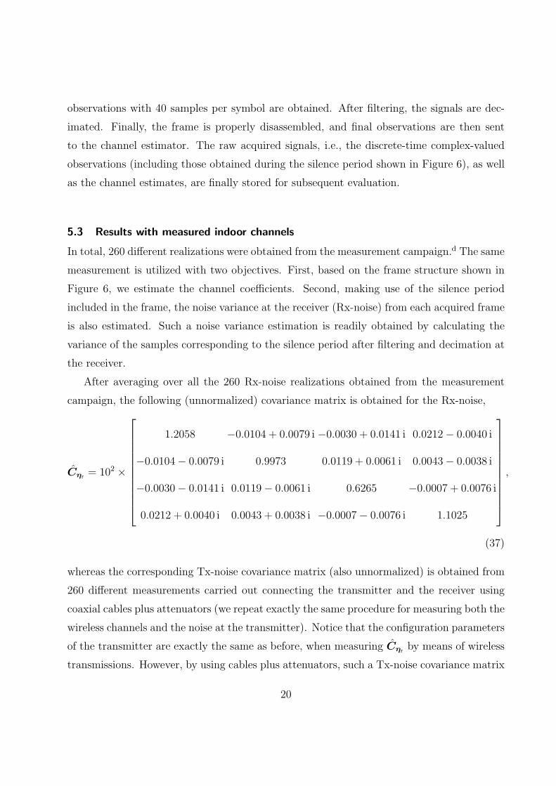
After averaging over all the 260 Rx-noise realizations obtained from the measurement

campaign, the following (unnormalized) covariance matrix is obtained for the Rx-noise,

Cηr = 102 ×

1.2058 −0.0104 + 0.0079 i −0.0030 + 0.0141 i 0.0212− 0.0040 i

−0.0104− 0.0079 i 0.9973 0.0119 + 0.0061 i 0.0043− 0.0038 i

−0.0030− 0.0141 i 0.0119− 0.0061 i 0.6265 −0.0007 + 0.0076 i

0.0212 + 0.0040 i 0.0043 + 0.0038 i −0.0007− 0.0076 i 1.1025

,

(37)

whereas the corresponding Tx-noise covariance matrix (also unnormalized) is obtained from

260 different measurements carried out connecting the transmitter and the receiver using

coaxial cables plus attenuators (we repeat exactly the same procedure for measuring both the

wireless channels and the noise at the transmitter). Notice that the configuration parameters

of the transmitter are exactly the same as before, when measuring Cηr by means of wireless

transmissions. However, by using cables plus attenuators, such a Tx-noise covariance matrix

20

estimation is significantly more accurate as well as more precise because the channel matrix

H in Equation (36) can be assumed to be known (actually, the cabled channel is estimated

with very high precision and accuracy). Such a Tx-noise covariance matrix is given by

Cηt = 10−3 ×

2.6069 0.0810− 0.0115 i 0.0058 + 0.0068 i −0.0107 + 0.0001 i

0.0081 + 0.0115 i 2.6413 0.0020 + 0.0020 i −0.0127 + 0.0035 i

0.0058− 0.0068 i 0.0020− 0.0020 i 2.5552 0.0037 + 0.0018 i

−0.0107− 0.0001 i −0.0127− 0.0035 i 0.0037− 0.0018 i 3.4155

.

(38)

Thus, the STxNR is estimated by performing Nt/ tr(Cηt), with Cηt given by Equation (38),

obtaining as a result the value of 25.52 dB, which is in accordance with the practical range

between 22 dB and 32 dB.

The figure of merit chosen for the performance evaluation is the uncoded BER versus

SRxNR, as defined in Equation (3). The symbols are QPSK modulated and it is also

assumed that Cu = I. The channel is quasi-static and remains unchanged during the

transmission of a frame of 105 symbols. Therefore, additive Gaussian Rx-noise and Tx-noise

were artificially generated and spatially colored according to matrices of Equations (37)

and (38), respectively, to recreate the measured scenario. Also note that additional noise

was injected to change the operating SRxNR value of the BER curves.

Figures 7 to 10 show the results after averaging over all the 260 channel realizations ob-

tained from this measurement campaign. Each figure plots the uncoded BER versus SRxNR

curves corresponding to the following three different situations: i) system performance for the

ideal case in which there is no Tx-noise (curves labeled as “Classical . . . with no Tx-noise”);

ii) system performance when there is Tx-noise but the system design does not take it into

account (curves labeled as “Classical . . . with Tx-noise”); and iii) system performance when

there is Tx-noise which is considered for the system design (curves labeled as “Modified . . .

with Tx-noise”).

Figure 7 shows the performance of the MIMO system with both MMSE and ZF linear

receivers. As it can be seen from the figure, linear receivers are very little affected by the

21

presence of Tx-noise. Figure 7 also plots the average BER versus SRxNR for MIMO systems

with both MMSE DF and ZF DF receivers. Again, Tx-noise does not severely degrade system

performance (except for the MMSE DF at SRxNR values greater than 30 dB). Considering

the Tx-noise in the DF receiver design only produces a small improvement in performance.

TX-noise, however, severely degrades the performance of MIMO systems with linear

precoding (LP), as it is plotted in Figure 8. Notice how performance starts to degrade for

SRxNR values above 20 dB. Tx-noise causes an error floor of about 10−2, which can be

reduced to 3× 10−3 when it is considered in the MMSE precoder design.

Figure 9 plots the BER performance in terms of SRxNR for MIMO systems with both

MMSE and ZF TH precoding. Note the high sensitivity of the performance of MIMO

systems with THP with respect to Tx-noise, which produces that the curves go up again for

high scenarios [31]. The performance of both MMSE and ZF TH precoding is considerably

degraded due to the Tx-noise and an error floor arises at the significant value of 2 × 10−3

(at 40 dB of SRxNR). This error floor reduces to about 2× 10−6 (at 40 dB of SRxNR) when

the Tx-noise is considered in the THP design. Therefore, the increasing effect in BER due

to Tx-noise, specially for high SNR, is strongly mitigated when the design is robust against

this type of impairments.

The same behaviour is observed for VP although at lower values of BER since VP per-

forms better than THP and it is not so influenced by noise impairments at the transmitter

due to the correction performed by the lattice search. Figure 10 shows how Tx-noise de-

grades the performance of MIMO systems with MMSE VP for SRxNR values greater than

20 dB introducing an error floor at 10−5. This error floor reduces to 2 × 10−6 when the

Tx-noise is introduced in the MMSE VP design.

In general, in all cases—linear precoding, Tomlinson-Harashima, and vector precoding—

for SRxNR values smaller than 20 dB, the noise at the receiver is the dominant factor, so

that STxNR values around 25 dB do not influence the uncoded BER performance. Note

that the STxNR value of 25.52 dB determines the SRxNR value at which the performance

begins to be improved by considering Tx-noise in the system design.

Figures 9 and 10 present the performance evaluation results in terms of uncoded BER

versus SRxNR for TH precoding as well as VP when QPSK mappings are utilized. However,

22

higher modulation levels lead to a greater loss in performance when the Tx-noise is not

included in the designs as it can be seen in Figures 11 and 12, where the performance of

Tomlinson-Harashima and vector precoding using 16-QAM is, respectively, shown. In both

cases, the proposed modified designs will mitigate that loss produced by Tx-noise.

Finally, note also that for increasing SRxNR values, all curves corresponding to MMSE-

based systems converge to those corresponding to ZF-based systems.

6 Conclusions

This study investigates the impact of transmitter noise on the performance of several

MIMO systems, namely, linear and decision feedback receivers, as well as linear, Tomlinson-

Harashima, and vector precoders. In all these cases, both MMSE and ZF designs were

considered. We derived the expressions for all the transceiver designs taking into account

the presence of transmitter noise. We also presented the results that illustrate the per-

formance of all the aforementioned transmission schemes using MIMO channels and noise

models, both obtained from an indoor measurement campaign carried out with a MIMO

testbed developed at the University of A Coruna.

Basically, we conclude that transmitter noise has little impact on the performance—

expressed in terms of uncoded BER versus signal-to-noise ratio at the receiver—of MIMO

linear and decision feedback receivers, but marginal performance improvements can be ex-

pected when considering transmitter noise in the receiver design. On the contrary, transmit-

ter noise considerably degrades the performance of precoded MIMO systems. Nevertheless,

significant improvements on performance are obtained when transmitter noise is included in

the precoder design. As expected, systems with VP produce the best results while the worst

ones are obtained with LP.

Competing interests

The authors declare that they have no competing interests.

23

Acknowledgments

This study has been funded by Xunta de Galicia, Ministerio de Ciencia e Innovacion of

Spain, and FEDER funds of the European Union under grants with numbers 10TIC003CT,

09TIC008105PR, TEC2010-19545-C04-01, and CSD2008-00010.

Appendix 1: Details of robust optimizations

In this appendix, we will derive the expressions of all the linear and nonlinear filters shown

throughout this article including the transmitter noise in the optimizations in order to obtain

the MMSE robust designs appropriate to mitigate such transmitter impairments.

Appendix 1.1: Derivation of MIMO linear receiver design with transmitter noise

The mean square error with Tx-noise in the MMSE linear receiver design is given by

E[∥ϵt[n]∥22

]= tr (Cu)− tr

(p∗CuH

HGH)− tr (pGHCu)

+ tr(|p|2 GHCuH

HGH)+ tr

(GCηrG

H)+ tr(GHCηtH

HGH),

which can be expressed similarly to Equation (9) by doing E[∥ϵ[n]∥22

], i.e., the mean

square error without Tx-noise, equal to tr (Cu) − tr(p∗CuH

HGH)− tr (pGHCu) +

tr(|p|2 GHCuH

HGH)+ tr

(GCηrG

H).

Then, we construct the Lagrangian function as follows

Lt (p,G, λ) = E[∥ϵt[n]∥22

]+ λ

(|p|2 tr (Cu)− Etx

),

with the Lagrangian multiplier λ ∈ R0,+.

We equate the derivatives with respect to p and G to zero, which leads to the following

24

Karush-Kuhn-Tucker (KKT) optimality conditions [32–35]

∂Lt (•)∂G∗ = −p∗CuH

H + |p|2GHCuHH +GHCηtH

H +GCηr = 0

∂Lt (•)∂p

= − tr (GHCu) + p∗ tr(GHCuH

HGH)+ λp∗ tr (Cu) = 0

|p|2 tr (Cu) ≤ Etx

λ(|p|2 tr (Cu)− Etx

)= 0 with λ ≥ 0.

From the first equation, we obtain the following expression for the receive filter G

G = p∗CuHH(|p|2 HCuH

H +Cηr +HCηtHH)−1

.

By plugging this result into the second KKT condition, it is easy to demonstrate that λ > 0,

and therefore the energy transmit constraint is maintained. To ensure a unique solution, we

restrict p ∈ R+. Thus, p is obtained from the energy transmit constraint and we have that

p =√

Etx

tr(Cu). Applying the matrix inversion lemma to the above expression for the receive

filter GMMSE, it can be demonstrated that

GMMSE = pMMSECuHH(C−1

η −C−1η H

(p−2MMSEI +CuH

HC−1η H

)−1CuH

HC−1η

)= pMMSE

(Cu −CuH

HC−1η H

(p−2MMSEI +CuH

HC−1η H

)−1Cu

)HHC−1

η

= pMMSE

(C−1

u + p2MMSEHHC−1

η H)−1

HHC−1η ,

where Cη = Cηr +HCηtHH .

Then, we easily reach the solution for the MMSE linear receiver in Equation (10).

Appendix 1.2: Derivation of MIMO linear precoder design with transmitter noise

The mean square error for the MMSE linear precoder design with Tx-noise is given by

E[∥ϵt[n]∥22

]= tr (Cu)− tr

(g∗CuF

HHH)− tr (gHFCu)

+ |g|2 tr(HFCuF

HHH)+ |g|2 tr (Cηr) + |g|2 tr

(HCηtH

H), (39)

25

where it can be equated E[∥ϵ[n]∥22

]= tr (Cu) − tr

(g∗CuF

HHH)− tr (gHFCu) +

|g|2 tr(HFCuF

HHH)+ |g|2 tr (Cηr) according to Equation (15).

Thus, we can form the following Lagrangian function

Lt (F , g, λ) = E[∥ϵt[n]∥22

]+ λ

(tr(FCuF

H)− Etx

).

Setting the derivatives with respect to F and g to zero, we obtain the necessary KKT

conditions

∂Lt (•)∂F ∗ = −g∗HHCu + |g|2 HHHFCu + λFCu = 0

∂Lt (•)∂g

= − tr (HFCu) + g∗ tr(HFCuF

HHH)

+ g∗ tr (Cηr) + g∗ tr(HCηtH

H)= 0

tr(FCuF

H)≤ Etx

λ(tr(FCuF

H)− Etx

)= 0 with λ ≥ 0. (40)

The gain g∗ obtained from the second equation is given by

g∗ =tr (HFCu)

tr (HFCuF HHH +HCηtHH +Cηr)

. (41)

Multiplying the first KKT condition by F H from the right and applying the trace operator,

we get the following

g∗ tr(HHCuF

H)− |g|2 tr

(HFCuF

HHH)= λ tr

(FCuF

H).

And now, combining this result with the expression for g∗ in Equation (41) yields

λ tr(FCuF

H)=

tr (HFCu)

tr (HFCuFHHH +HCηtHH +Cηr)

tr(HHCuF

H)

− |tr (HFCu)|2

tr2 (HFCuF HHH +HCηtHH +Cηr)

tr(HFCuF

HHH)

= |g|2 tr(Cηr +HCηtH

H). (42)

26

From the above result λ = |g|2 ξt, and if we plug this result for λ into the first KKT

condition, we get

F =1

g

(HHH + ξtI

)−1HH. (43)

By considering tr(FCuFH) = Etx and the above expression for F , it is obtained that

|g|2 =tr((

HHH + ξtI)−2

HHCuH)

Etx

,

which leads to a unique solution given by Equation (16) if we restrict g to being positive

real.

Appendix 1.3: Derivation of MIMO decision feedback receiver design with transmitter

noise

The mean square error is calculated as

E[∥ϵt,p[n]∥22

]= tr

(BPCuP

TBH)− tr

(BPCuH

HGH)− tr

(GHCuP

TBH)

+ tr(GHCuH

HGH)+ tr

(GCηrG

H)+ tr

(GHCηtH

HGH), (44)

where E[∥ϵp[n]∥22

]of Equation (20) is given by E

[∥ϵp[n]∥22

]= tr

(BPCuP

TBH)−

tr(BPCuH

HGH)− tr

(GHCuP

TBH)+ tr

(GHCuH

HGH)+ tr

(GCηrG

H).

This allows us to construct the Lagrangian function

Lt (P ,G,B,µ1, . . . ,µk) = E[∥ϵt[n]∥22

]+ 2ℜ

(tr

(N∑i=1

(eTi BST

i − eTi S

Ti

)µi

)), (45)

where the equality eTi BST

i = eTi S

Ti , for i = 1, . . . , N , must hold because of the unit lower

triangular structure of B.e To mathematically formulate this restriction, we included the

selection matrix Si defined as

Si = [0N−i+1×i−1, IN−i+1] ∈ {0, 1}N−i+1×N . (46)

The Lagrangian multiplier µi, i = 1, . . . , N , is a column vector of dimension N − i+ 1.

27

By setting its derivatives with respect to G and B to zero, we obtain the following KKT

conditions

∂Lt (•)∂G∗ = −BPCuH

H +GHCuHH +GHCηtH

H +GCηr = 0

∂Lt (•)∂B∗ = BPCuP

T −GHCuPT +

N∑i=1

eiµHi Si = 0

eTi BST

i = eTi S

Ti ∀i ∈ {1, . . . , N}. (47)

From the second KKT condition, we obtain

B = GHP T −

(N∑i=1

eiµHi Si

)PC−1

u P T. (48)

Plugging this expression for B into the first KKT condition, we get

G = −

(N∑i=1

eiµHi Si

)PHH

(HCηtH

H +Cηr

)−1. (49)

Substituting into Equation (48) we obtain

B = −

(N∑i=1

eiµHi Si

)P(HH

(HCηtH

H +Cηr

)−1H +C−1

u

)P T. (50)

Applying the restriction concerned with the unit lower triangular structure ofB to the above

result leads to

eTi BST

i = −eTi

(N∑j=1

ejµHj Sj

)P(HH

(HCηtH

H +Cηr

)−1H +C−1

u

)P TST

i = eTi S

Ti .

Then, with eTi ej = 0, for j = i, and 1, otherwise, µH

i reads as

µHi = −eT

i STi

[SiP

(HH

(HCηtH

H +Cηr

)−1H +C−1

u

)P TST

i

]−1

.

28

This result for µHi gives us the following expressions for the filters G and B

G =N∑i=1

eieTi S

Ti

[SiP

(HH

(HCηtH

H +Cηr

)−1H +C−1

u

)P TST

i

]−1

×

× SiPHH(HCηtH

H +Cηr

)−1

B =N∑i=1

eieTi S

Ti

[SiP

(HH

(HCηtH

H +Cηr

)−1H +C−1

u

)P TST

i

]−1

×

× SiP(HH

(HCηtH

H +Cηr

)−1H +C−1

u

)P T. (51)

Bearing in mind the Cholesky factorization with symmetric permutation, the feedforward

filter in Equation (51) reduces to

G =N∑i=1

eieTi S

Ti

(SiL

−HD−1L−1STi

)−1SiPHH

(HCηtH

H +Cηr

)−1

=N∑i=1

eieTi S

Ti

(SiL

−HD−1STi SiL

−1STi

)−1SiPHH

(HCηtH

H +Cηr

)−1

=N∑i=1

eieTi S

Ti SiLST

i SiDLHSTi SiPHH

(HCηtH

H +Cηr

)−1

=N∑i=1

eieTi DLHST

i SiPHH(HCηtH

H +Cηr

)−1=

N∑i=1

eieTi DLHPHHC−1

η

= DLHPHH(HCηtH

H +Cηr

)−1, (52)

where in the derivations we have used the following properties for the selection matrix Si

SiN = SiNSTi Si, eT

i STi SiMST

i Si = eTi , and eT

i NSTi Si = eT

i N ,

with N being an upper triangular matrix and M a unit lower triangular matrix. Comparing

this result with Equation (49) leads to the conclusion that −∑N

i=1 eiµHi Si = DLH. Hence,

the feedback filter reduces to

B = DLHL−HD−1L−1 = L−1. (53)

Therefore, the filters B and G corresponding to the MMSE DF receiver solution are given

by Equation (21).

29

Appendix 1.4: Derivation of MIMO Tomlinson-Harashima design with transmitter

noise

The mean square error is given by

E[∥ϵt[n]∥22

]= tr

(P TBCvB

HP)− g∗ tr

(P TBCvF

HHH)− g tr

(HFCvB

HP)

+ |g|2 tr(HFCvF

HHH)+ |g|2 tr (Cηr) + |g|2 tr

(HCηtH

H), (54)

where the mean square error without taking into account in the optimizations the Tx-noise

is given by E[∥ϵ[n]∥22

]= tr

(P TBCvB

HP)−g∗ tr

(P TBCvF

HHH)−g tr

(HFCvB

HP)+

|g|2 tr(HFCvF

HHH)+ |g|2 tr (Cηr) accordingly to Equation (25).

Then, the MSE in Equation (54) enables us to construct the Lagrangian function as

follows

Lt (P ,B,F , g, λ,µ1, . . . ,µK) = E[∥ϵt[n]∥22

]+ λ

(tr(FCvF

H)− Etx

)+ 2ℜ

(K∑i=1

tr(µT

i (SiBei − Siei)))

, (55)

where Si is a selection matrix defined as [cf. Equation (46)], λ ∈ R0,+, µi ∈ Ci, i = 1, . . . , K,

and 2ℜ(∑K

i=1 tr(µTi (SiBei−Siei))) comes from the restriction for the unit lower triangular

structure of the feedback matrix B.

Setting the derivatives of the Lagrangian function with respect to B, F , and g to zero

30

we obtain

∂Lt (•)∂F ∗ = −g∗HHP TBCv + |g|2HHHFCv + λFCv = 0

∂Lt (•)∂B∗ = BCv − gPHFCv +

K∑i=1

STi µ

∗ie

Ti = 0

∂Lt (•)∂g

= − tr(HFCvB

HP)+ g∗ tr

(HFCvF

HHH)

+ g∗ tr(HCηtH

H)+ g∗ tr (Cηr) = 0

SiBei = Siei

tr(FCvF

H)≤ Etx

λ(tr(FCvF

H)− Etx

)= 0 with λ ≥ 0. (56)

The weight g∗ resulting from the third KKT condition is expressed as

g∗ =tr(HFCvB

HP)

tr (HFCvF HHH +Cηr +HCηtHH)

. (57)

If we multiply the first KKT condition from the right by FH and afterwards apply the

trace operator we get

λ tr(FCvF

H)= g∗ tr

(HHP TBHCvF

H)− |g|2 tr

(HFCvF

HHH).

Plugging Equation (57) into the above equation, we can easily derive that

λ tr(FCvF

H)= |g|2 tr

(Cηr +HCηtH

H),

and then, λ = |g|2 tr(Cηr + HCηtHH)/ tr(FCvF

H) > 0 if we omit the trivial solution

F = 0. Therefore, the transmit energy constraint is active, i.e., tr(FCvFH) = Etx and

λ = |g|2 ξt with ξt = tr(Cηr +HCηtHH)/Etx, as before.

Thus, the resulting feedforward filter F obtained from the first equality in Equation (56)

is given by

F =1

g

(HHH + ξtI

)−1HHP TB =

1

gHH

(HHH + ξtI

)−1P TB, (58)

31

where we applied the matrix inversion lemma to get the last equality.

By plugging the above result into the second KKT condition, we obtain that

∂Lt (•)∂B∗ = BCv − PHHH

(HHH + ξtI

)−1P TBCv +

K∑i=1

STi µ

∗ie

Ti

= ξtP(HHH + ξtI

)−1P TBCv +

K∑i=1

STi µ

∗ie

Ti = 0.

Therefore, the feedback filter B is expressed as

B = −ξ−1t P

(HHH + ξtI

)P T

K∑i=1

STi µ

∗ie

Ti σ

−2v,i , (59)

where we included the assumption that the entries of v[n] are uncorrelated.

Multiplying this result by Si from the left and by ei from the right, we have

SiBei = −ξ−1t SiP

(HHH + ξtI

)P TST

i µ∗iσ

−2v,i = Siei.

Then, the Lagrangian multipliers µ∗i , i = 1, . . . , K are given by

µ∗i = −σ2

v,iξt(SiP

(HHH + ξtI

)P TST

i

)−1Siei. (60)

We can now substitute µ∗i of Equation (60) into Equations (58) and (59) so we have the

following expressions for the feedforward and feedback filters

F =1

gHHP T

K∑i=1

STi

(SiP

(HHH + ξtI

)P TST

i

)−1Sieie

Ti

B = P(HHH + ξtI

)P T

K∑i=1

STi

(SiP

(HHH + ξtI

)P TST

i

)−1Sieie

Ti , (61)

respectively.

Taking into account the Cholesky factorization, the precoder filters in Equation (61) can

32

be rewritten as

F =1

gTHPMMSE

HHP T

K∑i=1

STi

(SiL

−1D−1L−HSTi

)−1Sieie

Ti

=1

gTHPMMSE

HHP T

K∑i=1

STi SiL

HSTi SiDLST

i SieieTi

=1

gTHPMMSE

HHP T

K∑i=1

STi SiL

HSTi SiDLeie

Ti

=1

gTHPMMSE

HHP T

K∑i=1

STi SiL

HDeieTi =

1

gTHPMMSE

HHP TLHD

B = L−1D−1L−HLHD = L−1,

by considering the following properties of the selection matrix Si

SiM = SiMSTi Si, ST

i SiMei = ei and STi SiNei = Nei, (62)

with M being a unit lower triangular matrix and with N having an upper triangular struc-

ture. These results for F and B are shown in Equation (28).

Appendix 1.5: Derivation of MIMO vector precoder design with transmitter noise

The mean square error is given by

MSEt,VP =1

NB

NB∑n=1

(dH[n]d[n]− g∗xH[n]HHd[n]− gdH[n]Hx[n]

+ |g|2 xH[n]HHHx[n] + |g|2 tr (Cηr) + |g|2 tr(HCηtH

H))

, (63)

where MSEVP = 1NB

∑NB

n=1

(dH[n]d[n]− g∗xH[n]HHd[n]− gdH[n]Hx[n] + |g|2 xH[n]HHHx[n]

+ |g|2 tr (Cηr))accordingly to Equation (33) defines the mean square error when the trans-

mitter noise is not included in the filter optimizations.

The Lagrangian function can be expressed as

Lt (a[n],x[n], g, λ) = MSEt,VP + λ

(1

NB

NB∑n=1

xH[n]x[n]− Etx

), (64)

33

where λ ∈ R0,+. Now, we set its derivative with respect to x[n] and g to zero

∂Lt (•)∂x∗[n]

=1

NB

(−g∗HHd[n] + |g|2HHHx[n]

)+

λ

NB

x[n] = 0

∂Lt (•)∂g

=1

NB

(−dH[n]Hx[n] + g∗xH[n]HHHx[n]

+g∗ tr(HCηtH

H)+ g∗ tr (Cηr)

)= 0

1

NB

NB∑n=1

xH[n]x[n] ≤ Etx

λ

(1

NB

NB∑n=1

xH[n]x[n]− Etx

)= 0 with λ ≥ 0. (65)

Then, the transmit symbols are directly obtained from the first KKT condition and are

given by

x[n] =1

g

(HHH +

λ

|g|2I

)−1

HHd[n]. (66)

First of all, we have to show that λ > 0, i.e., the power constraint as active. Multiplying

the second KKT condition by g, we have

1

NB

(−gdH[n]Hx[n] + |g|2 xH[n]HHHx[n] + |g|2 tr (Cηr) + |g|2 tr

(HCηtH

H))

= 0, (67)

and multiplying the Hermitian of the first KKT condition by x[n] from the right, we have

1

NB

(−gdH[n]Hx[n] + |g|2 x[n]HHHHx[n]

)+

λ

NB

xH[n]x[n] = 0. (68)

With Equation (67) and the transmit energy constraint, the Lagrangian multiplier λ is given

by

λ = |g|2tr(Cηr +HCηtH

H)

1NB

∑NB

n=1 xH[n]x[n]

. (69)

Therefore, it becomes clear that λ > 0 for the non-trivial case that ∃n : x[n] = 0. Thus,

the transmit energy constraint is active, λ = |g|2 ξt, and gVPMMSE is directly obtained from the

transmit energy constraint.

Then we reach the solution for the MMSE VP in Equation (34).

Applying the matrix inversion lemma to Equation (34) shows that xVPMMSE[n] =

1gVPMMSE

HHΦtd[n] and then, gVPMMSE =

√∑NB

n=1(dH[n]ΦH

t HHHΦtd[n])/(EtxNB). Thus, when

34

we plug these results into the MSE expression in Equation (63) we obtain that

MSEt,VP =ξtNB

NB∑n=1

dH[n]Φtd[n]. (70)

SinceΦt is positive definite, we can use the Cholesky factorization to obtain a lower triangular

matrix L and a diagonal matrix D with the following relationship

Φt =(HHH + ξtI

)−1= LHDL.

Thus, the perturbation signal can be found by search in Equation (35)

Endnotes

aIn the particular case of QPSK modulation, τ = 2√2. bIn our measurements, we use

monopole, dual-band antennas [36]. cWe have previously calibrated our front-ends so when

we scale the passband signals prior to the DACs we ensure that the mean transmit power

is fixed regardless of the RF carrier frequency utilized. We also ensure that the power

amplifiers at the transmitter are operating in their linear region (note that the front-ends

have an output IP3 of 25 dBm per antenna in the 5GHz band and of 37.5 dBm in the 2.5GHz

band). dAll measurement results (including the channel coefficients and the corresponding

covariance matrices for the Tx-noise as well as for the Rx-noise are available on request).

eThe lefthand side cuts out the last N− i+1 elements of the ith row of B and the righthand

side sets the first of those elements (the ith diagonal element of B) to one and the others to

zero (triangularity of B).

References

1. H Suzuki, T Tran, I Collings, G Daniels, M Hedley, Transmitter noise effect on the

performance of a MIMO-OFDM hardware implementation achieving improved coverage.

IEEE J. Sel. Areas Commun. 26(6), 867–876 (2008)

35

2. C Studer, M Wenk, A Burg, MIMO transmission with residual Tx-RF impairments,

in Proc. of International ITG Workshop Smart Antennas, 2010, pp. 189–196, Bremen,

Germany

3. M Joham, W Utschick, JA Nossek, Linear transmit processing in MIMO communications

systems. IEEE Trans. Signal Process. 53(8), 2700–2712 (2005)

4. JA Nossek, M Joham, W Utschick, Transmit processing in MIMO wireless systems,

in Proc. of the 6th IEEE Circuits and Systems Symposium on Emerging Technologies:

Frontiers of Mobile and Wireless Communication, Shanghai, China, vol. 1, 2004, pp.

I–18–I–23

5. M Joham, Optimization of Linear and Nonlinear Transmit Signal Processing. PhD dis-

sertation. Munich University of Technology, 2004

6. RL Choi, RD Murch, New transmit schemes and simplified receiver for mimo wireless

communication systems. IEEE Trans. Wirel. Commun. 2(6), 1217–1230 (2003)

7. HR Karimi, M Sandell, J Salz, Comparison between transmitter and receiver array

processing to achieve interference nulling and diversity, in Proc. of PIMRC, vol. 3, 1999,

pp. 997–1001, Osaka, Japan

8. M Joham, K Kusume, MH Gzara, W Utschick, JA Nossek, Transmit wiener filter for

the downlink of TDD DS-CDMA systems, in Proc. of ISSSTA, vol. 1, 2002, pp. 9–13,

Prague, Czech Republic

9. A Duel-Hallen, A family of multiuser decision-feedback detectors for asynchronous code-

division multiple-access channels. IEEE Trans. Commun. 43(2/3/4), 421–434 (1995)

10. N Al-Dhahir, A Sayed: The Finite-Length Multi-Input Multi-Output MMSE-DFE.

IEEE Trans. Signal Process. 48(10), 2921–2936 (2000)

11. RFH Fischer, Precoding and Signal Shaping for Digital Transmission (John Wiley &

Sons, Hoboken, New York, USA, 2002)

36

12. K Kusume, M Joham, W Utschick, G Bauch, Cholesky factorization with symmetric

permutation applied to detecting and precoding spatially multiplexed data streams.

IEEE Trans. Signal Process. 55(6), 3089–3103 (2007)

13. DA Schmidt, M Joham, W Utschick, Minimum mean square error vector precoding. Eur.

Trans. Telecommun. 19(3), 219–231 (2008)

14. J Gonzalez-Coma, P Castro, L Castedo, Impact of transmit impairments on multiuser

MIMO non-linear transceivers, in Proc. of International ITG Workshop on Smart An-

tennas (WSA), 2011, pp. 1–8, Aachen, Germany

15. J Gonzalez-Coma, P Castro, L Castedo, Transmit impairments influence on the perfor-

mance of MIMO receivers and precoders, in Proc. of European Wireless (EW), 2011, pp.

1–8, Vienna, Austria

16. J Gonzalez-Coma, P Castro, JA Garcıa-Naya, L Castedo, Performance evaluation of

non-linear MIMO precoders under transmit impairments, in Proc. 19th European Signal

Processing Conference, 2011, Barcelona, Spain

17. JA Garcıa-Naya, M Gonzalez-Lopez, L Castedo: Radio Communications, INTECH 2010

chap. A Distributed Multilayer Software Architecture for MIMO Testbeds

18. FP6-IST project MASCOT. http://www.ist-mascot.org

19. A Behzad, Wireless LAN Radios (John Wiley & Sons, Hoboken, New Jersey, USA, 2007)

20. C Windpassinger, RFH Fischer, T Vencel, JB Huber, Precoding in Multiantenna and

Multiuser Communications. IEEE Trans. Wirel. Commun. 3(4), 1305–1316 (2004)

21. GK Kaleh, Channel equalization for block transmission systems. IEEE J. Sel. Areas

Commun. 13, 110–121 (1995)

22. K Kusume, M Joham, W Utschick, MMSE block decision-feedback equalizer for spa-

tial multiplexing with reduced complexity, in Proc. IEEE Global Telecommunications

Conference, vol. 4, Dallas, Texas, USA, 2004, pp. 2540–2544

37

23. CP Schnorr, M Euchnerr, Lattice basis reduction: improved practical algorithms and

solving subset sum problems. Math. Program. 66, 188–191 (1994)

24. JA Garcıa-Naya, O Fresnedo, FJ Vazquez-Araujo, M Gonzalez-Lopez, L Castedo, J

Garcia-Frias, Experimental evaluation of analog joint source-channel coding in indoor

environments, in Proc. IEEE International Conference on Communications (ICC), Ky-

oto, Japan, 2011, pp. 1–5

25. O Gonzalez, D Ramırez, I Santamarıa, JA Garcıa-Naya, L Castedo, Experimental val-

idation of interference alignment techniques using a multiuser MIMO testbed, in Proc.

International ITG Workshop on Smart Antennas (WSA), Aachen, Germany, 2011, pp.

1–8

26. Lyrtech, Inc., 2011. http://www.lyrtech.com

27. Maxim Integrated Products, Inc., 2011. http://www.maxim-ic.com/

28. Ettus Research, LLC, 2011. http://www.ettus.com

29. Sundance Multiprocessor, Ltd., 2011. http://www.sundance.com

30. S Caban, JA Garcıa Naya, M Rupp, Measuring the physical layer performance of wire-

less communication systems: part 33 in a series of tutorials on instrumentation and

measurement. IEEE Instru. Meas. Mag. 14(5), 8–17 (2011)

31. M Joham, P Castro, L Castedo, W Utschick, Robust Precoding with Bayesian Error

Modeling for Limited Feedback MU-MISO Systems. IEEE Trans. Signal Process. 58(9),

4954–4960 (2010)

32. W Karush, Minima of Functions of Several Variables with Inequalities as Side Condi-

tions. M.S. Thesis. The University of Chicago, 1939

33. R Fletcher, Practical Methods of Optimization, 2nd edition (John Wiley & Sons, UK,

2000)

34. DG Luenberger, Linear and Nonlinear Programming, 2nd edition (Kluwer Academic

Publishers, USA, 2004)

38

35. HW Kuhn, AW Tucker, Nonlinear Programming, in Proc. 2nd Berkeley Symposium on

Mathematical Statistics and Probability, J. Neyman, University of California Press, 1951,

pp. 481–492, Berkeley, CA, USA

36. L-Com Antenna No. HG2458RD-SM, 2010. http://www.l-com.com/item.aspx?id=22199

Figure 1.. MIMO linear transmit processing and linear receive processing with

Tx-noise.

Figure 2.. MIMO linear transmit processing and nonlinear receive processing

(DF) with Tx-noise.

Figure 3.. Nonlinear MIMO system with THP and Tx-noise.

39

Figure 4.. Nonlinear MIMO system with VP and Tx-noise.

Figure 5.. Picture of testbed transmitter developed at the University of A

Coruna.

Figure 6.. Frame structure used in the measurements.

Figure 7.. BER versus SRxNR with MIMO linear and nonlinear (DF) receivers

over measured indoor channels. Figure 7 shows the uncoded BER with respect to the

SRxNR. A MIMO system with four transmit antennas and four receive antennas (Nt =

Nr = 4) is considered. The performance evaluation is carried out for ZF as well as MMSE,

considering linear receivers and nonlinear (DF) receivers, while all schemes are evaluated

with and without Tx-noise. Finally, schemes specifically designed to deal with Tx-noise

(labeled as “modified”) are also evaluated. In all cases, QPSK signals over measured indoor

channels are used, whereas the estimated STxNR is about 25 dB.

Figure 8.. BER versus SRxNR with MIMO LP over measured indoor channels.

Figure 8 shows the uncoded BER with respect to the SRxNR. A MIMO system with four

transmit antennas and four receive antennas (Nt = Nr = 4) is considered. The performance

evaluation is carried out considering LP for ZF as well as MMSE, while all schemes are

evaluated with and without Tx-noise. Finally, schemes specifically designed to deal with Tx-

noise (labeled as “modified”) are also evaluated. In all cases, QPSK signals over measured

indoor channels are used, whereas the estimated STxNR is about 25 dB.

40

Figure 9.. BER versus SRxNR with MIMO THP over measured indoor channels.

Figure 9 shows the uncoded BER with respect to the SRxNR. A MIMO system with four

transmit antennas and four receive antennas (Nt = Nr = 4) is considered. The performance

evaluation is carried out considering THP for ZF as well as MMSE, while all schemes are

evaluated with and without Tx-noise. Finally, schemes specifically designed to deal with Tx-

noise (labeled as “modified”) are also evaluated. In all cases, QPSK signals over measured

indoor channels are used, whereas the estimated STxNR is about 25 dB.

Figure 10.. BER versus SRxNR with MIMO VP over measured indoor channels

for Nt = Nr = 4. Estimated STxNR is about 25 dB. Figure 10 shows the uncoded BER

with respect to the SRxNR. A MIMO system with four transmit antennas and four receive

antennas (Nt = Nr = 4) is considered. The performance evaluation is carried out considering

VP for ZF as well as MMSE, while all schemes are evaluated with and without Tx-noise.

Finally, schemes specifically designed to deal with Tx-noise (labeled as “modified”) are also

evaluated. In all cases, QPSK signals over measured indoor channels are used, whereas the

estimated STxNR is about 25 dB.

41

Figure 11.. The same as Figure 9 but for 16-QAM instead of QPSK. Figure 11

shows the uncoded BER with respect to the SRxNR. A MIMO system with four transmit

antennas and four receive antennas (Nt = Nr = 4) is considered. The performance evaluation

is carried out considering THP for ZF as well as MMSE, while all schemes are evaluated

with and without Tx-noise. Finally, schemes specifically designed to deal with Tx-noise

(labeled as “modified”) are also evaluated. In all cases, 16-QAM signals over measured

indoor channels are used, whereas the estimated STxNR is about 25 dB.

Figure 12.. The same as Figure 11 but for 16-QAM instead of QPSK. Figure 12

shows the uncoded BER with respect to the SRxNR. A MIMO system with four transmit

antennas and four receive antennas (Nt = Nr = 4) is considered. The performance evaluation

is carried out considering VP for ZF as well as MMSE, while all schemes are evaluated with

and without Tx-noise. Finally, schemes specifically designed to deal with Tx-noise (labeled as

“modified”) are also evaluated. In all cases, 16-QAM signals over measured indoor channels

are used, whereas the estimated STxNR is about 25 dB.

42

u[n]F

x[n]

ηt[n]

xt[n]

H

ηr[n]

yt[n]

linearprecoder

Gût[n]

Q( )u[n]~

linearreceiverFigure 1

u[n]F

x[n]

ηt[n]

xt[n]

H

ηr[n]

yt[n]

linearprecoder

Gû

t[n]

Q( )u[n]~

nonlinear receiver (DF)

I – B

P T

up[n]~

Figure 2

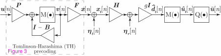
u[n]

ηt[n]

xt[n]

H

ηr[n]

Pû

t[n]

M( )u[n]~

Tomlinson-Harashima (TH) precoding

I – B

Fx[n]v[n]

gId

t[n]^

M( ) Q( )

Figure 3

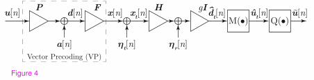
u[n]

ηt[n]

xt[n]

H

ηr[n]

Pût[n] u[n]~

Vector Precoding (VP)

Fx[n]

gIdt[n]^

M( ) Q( )

a[n]

d[n]

Figure 4

testbed

transmitter

4 x DAC output

RF front-end

40 MHz reference

oscillator input

Figure 5

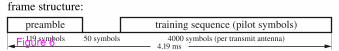
preamble training sequence (pilot symbols)

50 symbols119 symbols 4000 symbols (per transmit antenna)4.19 ms

frame structure:

Figure 6

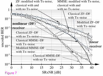
403530252015105010-6

10-5

10-4

10-3

10-2

10-1

1

SRxNR [dB]

uncoded B

ER

linear

receiver

MMSE: modified with Tx-noise,

classical with and

with no Tx-noise

ZF: modified with Tx-noise,

classical with and

with no Tx-noise

nonlinear (DF)

receiver

Encuukecn"¥H(FH"ykvj"Vz(pqkug

Oqfkhkgf"¥H(FH"ykvj"Vz(pqkug

Encuukecn"¥H(FH"ykvj"pq"Vz(pqkug

Encuukecn"OOUG/FHykvj"pq"Vz(pqkug

Oqfkhkgf"OOUG(FH"ykvj"Vz(pqkug

Encuukecn"OOUG(FH"ykvj"Vz(pqkug

Figure 7

4035302520151050

SRxNR [dB]

uncoded B

ER

10-6

10-5

10-4

10-3

10-2

10-1

1

Modified, classical

ZF LP with Tx-noise

Classical ZF LP

ykvj"pq"Vz(pqkug

Classical MMSE LP

ykvj"Vz(pqkug

Modified MMSE LP

ykvj"Vz(pqkugClassical MMSE LP

ykvj"pq"Vz(pqkug

Figure 8

403530252015105010-6

10-5

10-4

10-3

10-2

10-1

1

SRxNR [dB]

uncoded B

ER

Modified, classical

ZF THP with Tx-noise

Classical ZF THP

ykvj"pq"Vz(pqkug

Classical MMSE THP

ykvj"Vz(pqkug

Modified MMSE THP

ykvj"Vz(pqkug

Classical MMSE THP

ykvj"pq"Vz(pqkug

Figure 9

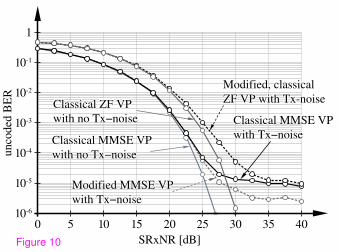
403530252015105010-6

10-5

10-4

10-3

10-2

10-1

1

SRxNR [dB]

uncoded B

ER

Modified, classical

ZF VP with Tx-noiseClassical ZF VP

ykvj"pq"Vz(pqkug Classical MMSE VP

ykvj"Vz(pqkug

Modified MMSE VP

ykvj"Vz(pqkug

Classical MMSE VP

ykvj"pq"Vz(pqkug

Figure 10

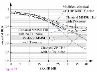
403530252015105010-6

10-5

10-4

10-3

10-2

10-1

1

SRxNR [dB]

uncoded B

ER

Modified, classical

ZF THP with Tx-noise

Classical ZF THP

ykvj"pq"Vz(pqkug

Classical MMSE THP

ykvj"Vz(pqkug

Modified MMSE THP

ykvj"Vz(pqkug

Classical MMSE THP

ykvj"pq"Vz(pqkug

Figure 11

10-6

10-5

10-4

10-3

10-2

10-1

1

4035302520151050

SRxNR [dB]

uncoded B

ER

Modified, classical

ZF VP with Tx-noise

Classical ZF VP

ykvj"pq"Vz(pqkug

Classical MMSE VP

ykvj"Vz(pqkug

Modified MMSE VP

ykvj"Vz(pqkug

Classical MMSE VP

ykvj"pq"Vz(pqkug

Figure 12