EUROPEAN JOURNAL OF PSYCHOTRAUMATOLOGY

BASIC RESEARCH ARTICLE

Analyzing small data sets using Bayesian estimation:the case of posttraumatic stress symptoms followingmechanical ventilation in burn survivors

Rens van de Schoot1,2*, Joris J. Broere1, Koen H. Perryck1,Marielle Zondervan-Zwijnenburg1 and Nancy E. van Loey3,4

1Department of Methods and Statistics, Utrecht University, Utrecht, The Netherlands; 2Optentia ResearchProgram, Faculty of Humanities, North-West University, Vanderbijlpark, South Africa; 3Department of Clinical& Health Psychology, Utrecht University, Utrecht, The Netherlands; 4Department Behavioural Research,Association of Dutch Burn Centres, Beverwijk, The Netherlands

Background: The analysis of small data sets in longitudinal studies can lead to power issues and often suffers

from biased parameter values. These issues can be solved by using Bayesian estimation in conjunction with

informative prior distributions. By means of a simulation study and an empirical example concerning

posttraumatic stress symptoms (PTSS) following mechanical ventilation in burn survivors, we demonstrate

the advantages and potential pitfalls of using Bayesian estimation.

Methods: First, we show how to specify prior distributions and by means of a sensitivity analysis we de-

monstrate how to check the exact influence of the prior (mis-) specification. Thereafter, we show by means

of a simulation the situations in which the Bayesian approach outperforms the default, maximum likelihood

and approach. Finally, we re-analyze empirical data on burn survivors which provided preliminary evidence

of an aversive influence of a period of mechanical ventilation on the course of PTSS following burns.

Results: Not suprisingly, maximum likelihood estimation showed insufficient coverage as well as power with

very small samples. Only when Bayesian analysis, in conjunction with informative priors, was used power

increased to acceptable levels. As expected, we showed that the smaller the sample size the more the results

rely on the prior specification.

Conclusion: We show that two issues often encountered during analysis of small samples, power and biased

parameters, can be solved by including prior information into Bayesian analysis. We argue that the use of

informative priors should always be reported together with a sensitivity analysis.

Keywords: Bayesian estimation; maximum likelihood; prior specification; power; repeated measures analyses; small samples;

burn survivors; mechanical ventilation; PTSS

Responsible Editor: Cherie Armour, University of Ulster, United Kingdom.

*Correspondence to: Rens van de Schoot, Department of Methods and Statistics, Utrecht University,

PO Box 80120, 3508TC, Utrecht, The Netherlands, Email: [email protected]

For the abstract or full text in other languages, please see Supplementary files under ‘Article Tools’

Received: 17 June 2014; Revised: 17 February 2015; Accepted: 20 February 2015; Published: 11 March 2015

‘‘The bigger the better, in everything,’’ Freddie

Mercury answered when he was asked if he

was intimidated by a large audience (Wigg,

2012). A statement highly contrasting to the famous motto

of Ludwig Mies van der Rohe: ‘‘less is more’’ (Mies van der

Rohe, 1994). Although both quotes had nothing to do

with statistics, they are representative for issues many

researchers have to deal with. The quote of Freddie

Mercury is highly applicable, because researchers in

many research areas are expected to work with large

sample sizes, especially in combination with complicated

statistical models. As is widely understood, the bigger

the sample size the higher the probability of finding

a significant result (Peto et al., 1976). However, a large

sample size is not always obtainable in any field of

research. A small sample size can be the consequence of

research protocols, a small research population, or when

it is ethically and morally unjustified to gather a larger

sample. When the sample is limited in size, it is, because

of power issues, often hard to get meaningful results

PSYCHOTRAUMATOLOGYEUROPEAN JOURNAL OF

�

European Journal of Psychotraumatology 2015. # 2015 Rens van de Schoot et al. This is an Open Access article distributed under the terms of the Creative CommonsAttribution 4.0 International License (http://creativecommons.org/licenses/by/4.0/), allowing third parties to copy and redistribute the material in any medium or format, andto remix, transform, and build upon the material, for any purpose, even commercially, under the condition that appropriate credit is given, that a link to the license is provided,and that you indicate if changes were made. You may do so in any reasonable manner, but not in any way that suggests the licensor endorses you or your use.

1

Citation: European Journal of Psychotraumatology 2015, 6: 25216 - http://dx.doi.org/10.3402/ejpt.v6.25216

(page number not for citation purpose)

http://www.eurojnlofpsychotraumatol.net/index.php/ejpt/rt/suppFiles/25216/0

http://creativecommons.org/licenses/by/4.0/

http://eurojnlofpsychotraumatol.net/index.php/ejpt/article/view/25216

http://dx.doi.org/10.3402/ejpt.v6.25216

(Button et al., 2013; Lee & Song, 2004; Price, 2012;

Scheines, Hoijtink, & Boomsma, 1999).

Hence, the question every researcher is faced with

‘‘How large should my sample be?’’ This question can

only be answered in relation to the number of parameters

included in a model (e.g., regression coefficients, inter-

cepts, residual variances). Lee and Song (2004) concluded

that when using maximum likelihood (ML) estimation

for structural equation models, sample sizes yield accu-

rate results when the ratio of parameters: sample size

is 1:5, whereas a 1:3 ratio produced some bias. This

ratio is less stringent than the rules of thumb often used

in practice, for example, 1:10 or 1:20. Of notice, the ratio

also depends on the model, the distribution of the

parameters/variables and other characteristics. As argued

by Muthen and Muthen (2002), the only way to answer

the sample size question is by performing a simulation

study. If a simulation study shows that a rule like 1:5

results in sufficient power, it would provide a starting

point for practical purposes.

However, what if the sample size based on such a ratio

is simply not feasible? Consider the hypothesis that burn

survivors who need mechanical ventilation in response

to inhalation injury have higher levels of posttraumatic

stress symptoms (PTSS) over time relative to burn sur-

vivors who do not need mechanical ventilation. In such

an example, obtaining a large sample is difficult in a

timely fashion because of the relatively low incidence of

burn injuries and particularly comorbid inhalation injury.

Approximately, 10% of burn patients admitted to a burn

center have inhalation injury (Belgian Outcome in Burn

Injury Study Group, 2009). Moreover, only a minority

of the patients develops PTSS (Van Loey & Van Son,

2003). According to a power study, 66 burn survivors

would be required of which half require mechanical

ventilation.1 To gather such a sample in small countries

like The Netherlands or Belgium would take many years.

It could be the case that, different underlying mechanisms

may play a role in the development and maintenance

of PTSS in those with and without ventilation. More-

over, different strategies may be required to treat or even

prevent this disorder. However, the power analysis tells

a researcher that in order to detect such a difference,

a sample size is needed that is, without an unreason-

able amount of time and resources, unattainable. Should

a researcher then simply ignore this research interest/

question? If the research is never carried out, then, a

possible important risk factor may be overlooked result-

ing in inadequate treatment with long term consequences

such as lower quality of life (Van Loey, Van Beeck, Faber,

Van de Schoot, & Bremer, 2012). Shouldn’t science also

aim at answering research questions of great importance

highly relevant for small research populations?

Because Bayesian analyses do not assume large samples,

as is the case with ML estimation, typically smaller data

sets can be analyzed without losing power while retaining

precision. As Lee and Song (2004) showed, Bayesian

estimation requires a much smaller ratio of parameters to

observations, namely for the models used in their paper

a ratio of 1:3 could be used instead of 1:5. Also Hox,

Van de Schoot, and Matthijsse (2012) showed with a

simulation study that using Bayesian estimation makes

it possible to use smaller data sets compared to ML

estimation (see also Hox, Moerbeek, Kluytmans, &

Van de Schoot, 2014).

Because the aim of our study is not to introduce

Bayesian statistics, we kindly refer readers who are

interested to the gentle introduction of Van de Schoot

et al. (2014), but see also Kaplan and Depaoli (2012),

Kruschke, Aguinis, and Joo (2012), or Zyphur and Oswald

(2015). For more technical details we refer to Gelman,

Carlin, Stern, and Rubin (2004). The heart of Bayesian

estimation is that everything that is known about a

parameter before observing the data (the prior) is com-

bined with the information from the data itself (the

likelihood), resulting in updated knowledge about the

parameter (the posterior). The prior information can

stem from a meta-analysis, previous studies with compar-

able research populations, a pilot study, experts, or a

range of other sources. If such knowledge is usedwe call the

prior informative, and if no knowledge is available (or used)

we call the prior non- or un-informative. It is debatable

when a prior is considered informative or un-informative,

therefore different statistical programs use different de-

fault settings regarding the un-informative priors. An

often used un-informative prior for variance terms is

an improper prior. An improper prior is a probability

distribution that does not sum up or integrate to one

(Jackman, 2009). Because it does not integrate or sum to

one, it can technically not serve as a probability distribution.

We return to this issue later in the article.

In the study of Lee and Song (2004) the authors

considered a situation in which, a priori, there was no

information available about the parameters of interest.

As such, un-informative prior distributions were specified

for the parameters in the model. Hence, the full potential

of the Bayesian toolbox was not used. Galindo-Garre,

Vermunt, and Bregsma (2004) specified an informative

prior and the authors concluded that the more informa-

tion is captured by the well-specified priors the smaller

the parameter bias. Also, (Depaoli, 2012) compared ML

estimation and the Bayesian framework, but she imple-

mented a wide range of priors: diffuse/un-informative

priors, ‘‘accurate’’ informative priors, weakly informative

1We estimated the power using a repeated measure model with three outcome

variables and regressing a dichotomous variable on the slope and parameters

based on the empirical data. For more information and the syntax files go to

the website of the first author.

Rens van de Schoot et al.

2(page number not for citation purpose)




priors, data-driven informative priors, priors reflecting

partial-knowledge of parameters, and ‘‘inaccurate’’ (but

informative) priors. The results indicated that optimal

parameter recovery was obtained through the Bayesian

approach using ‘‘accurate’’ informative priors, and partial-

knowledge priors showed promise for the recovery of

the growth trajectory parameters. Price (2012) compared

the small sample performance of a Bayesian versus a

frequentist time series model on power and parameter

estimation bias. Using informative priors, Price showed

the Bayesian approach provided better results for hypoth-

esis testing and detecting Type I error compared to ML.

We extended the work of the authors discussed above

in two ways. First, we investigate what influence the

amount of information captured by prior distributions

has on the ratios between the number of parameters

in the model and required sample size. Second, we con-

sider more extreme parameter to sample size rations.

We expect Bayesian estimation to give reliable results

with very small sample sizes if prior information is added

to the analyses.

In sum, our main objective of this study is to demon-

strate possibilities that exist for researching small popula-

tions through the use of Bayesian estimation, but as

we show the use of Bayesian statistics comes with a price.

That is, background information needs to be incorporated

in the analyses via the prior distribution. We demonstrate

(1) how to specify these priors; (2) how to investigate

the exact influence of the prior specification on the results

and conclusions; and (3) how much can be gained in terms

of sample size if more information is specified via the

priors. Throughout the paper a dataset concerning PTSS

in burn survivors is used as a case study to demonstrate

the advantages and pitfalls of using Bayesian statistics to

deal with small research populations. In particular, it was

investigated whether a period of unconsciousness during

mechanical ventilation would be associated with a differ-

ent course of PTSS. As the number of burn survivors

is limited we have to deal with a small sample size.

The structure of this paper is as follows: First, PTSS

in our sample is introduced and a description is given of

Repeated Measures ANOVA (RMA). Then we present

the results of the sensitivity analysis (Study 1) where

we investigate the influence of the prior specification on

the results. Thereafter, in a second study, we present a

simulation where we investigate the relationship between

the required sample size and the specification of the

prior distribution. Finally, the data on burn survivors is

analyzed. The data and syntax files for the sensitivity

analysis and the simulation study can be found on the

website of the first author.2

Empirical example

Posttraumatic stress disorderPosttraumatic stress disorder (PTSD) is a mental health

condition that can develop in the aftermath of exposure

to a traumatic event. It is one of the most common

psychiatric diagnoses in the general population after

trauma exposure (Breslau et al., 1998). PTSD includes

four symptoms clusters: intrusion, avoidance, negative

alterations in cognitions and mood, and alterations in

arousal and reactivity (American Psychiatric Association,

2013). A dysregulated fear response is considered an

important mechanism underlying PTSD. Fear condition-

ing is a complicated process in which a neutral condi-

tional stimulus becomes associated with an aversive

unconditioned stimulus (Parsons & Ressler, 2013). After

the fear conditioning the traumatic experience is con-

solidated in the memory. The consolidation period is a

time span directly followed after the trauma exposure;

this period could last minutes, hours, or even days

(Parsons & Ressler, 2013). Memory consolidation is a

process in which a transformation over time is going on

from short-term memory into long-term memory

(Schafe, Nader, Blair, & LeDoux, 2001). In recent years

interest has grown in factors that affect the consolidation

process (Baldi, Liuzzo, & Bucherelli, 2013; Datta &

O’Malley, 2013; Zohar, Juven-Wetzler, Myers, & Fostick,

2008). However, there is a paucity of studies investigating

whether a period of mechanical ventilation in which the

patient is brought into a state of unconsciousness, would

be associated with a different PTSD course over time. A

possible underlying mechanism may be that the consoli-

dation process during this period may be reinforced. A

recent review reported that three out of four studies

performed in ICU including a wide range of pathologies,

identified mechanical ventilation to be a risk factor for

PTSS (Wade, Hardy, Howell, & Mythen, 2013). Although

the results are currently inconclusive, possibly, the period

of ventilation may reinforce the consolidation process

during this period in such a way that the fear condition-

ing transforms more easily to a more permanent state

over time. As no studies are available in burn injured

populations, the research question of interest is whether

the development of PTSS in burn survivors who need

mechanical ventilation is different compared to burn

survivors who do not need mechanical ventilation.

MethodA subsample of the data from Van Loey, Maas, Faber,

and Taal (2003) was considered. Our subsample encom-

passed persons scoring above the cutoff point of clinically

relevant symptom levels measured 2 weeks post burn,

and for whom data on mechanical ventilation status was

available. Data were gathered in burn centers in the

2http://rensvandeschoot.com/433/additional-information-analyzing-small-data-

sets-using-bayesian-estimation.

Analyzing small data sets using Bayesian estimation

Citation: European Journal of Psychotraumatology 2015, 6: 25216 - http://dx.doi.org/10.3402/ejpt.v6.25216 3(page number not for citation purpose)

http://rensvandeschoot.com/433/additional-information-analyzing-small-data-sets-using-bayesian-estimation




Netherlands and Belgium between 1997 and 2003. Patients

admitted to a burn center were invited to participate in

a longitudinal study on PTSS. Patients with cognitive

disabilities, insufficient Dutch proficiency, and a length

of stay in hospital less than 72 hours were excluded.

Patients were invited to take part within 2 weeks post

burn by a local researcher and after providing written

informed consent, they completed questionnaires. Follow-

up questionnaires were sent to their home address.

Those requiring mechanical ventilation were included

into the study as soon as they gained consciousness and

were able to comprehend questions. The results were

described in Van Loey et al. (2003).

PTSS were measured using the Impact of Event Scale

(IES) (Horowitz, Wilner, & Alvarez, 1979). The IES is a

15-item self-report questionnaire used to assess intrusive

and avoidant symptoms associated with the experience

of a particular event. In this questionnaire, participants

are requested to rate statements like ‘‘I thought about

the burn event when I didn’t mean to’’, ‘‘I tried to remove

the burn event from memory’’ and ‘‘I had trouble falling

asleep or staying asleep because of pictures or thoughts

about the burn event that came into my mind’’. In this

study, the Dutch version of the IES was used (Brom

& Kleber, 1985). Responses were rated on a 0 (not at all)

to 100 (the worst imaginable way) visual analogue scale.

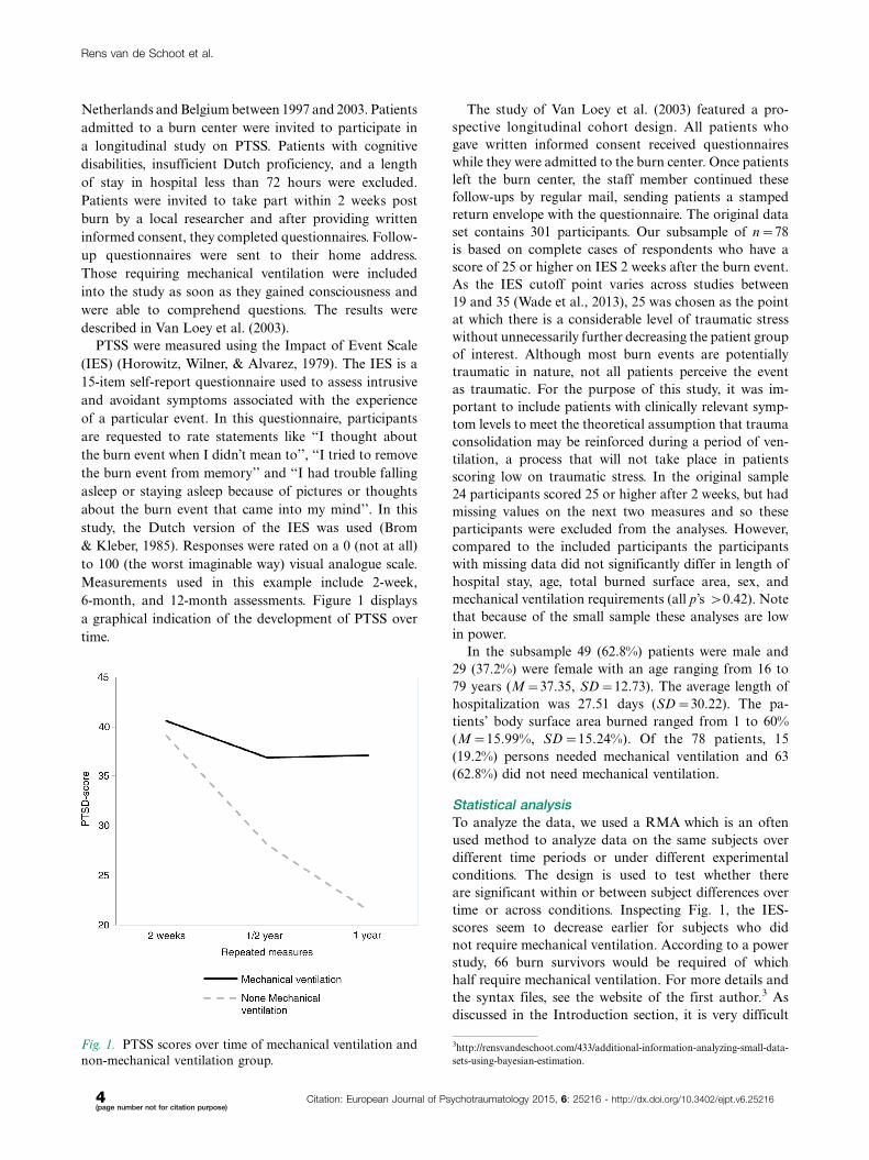
Measurements used in this example include 2-week,

6-month, and 12-month assessments. Figure 1 displays

a graphical indication of the development of PTSS over

time.

The study of Van Loey et al. (2003) featured a pro-

spective longitudinal cohort design. All patients who

gave written informed consent received questionnaires

while they were admitted to the burn center. Once patients

left the burn center, the staff member continued these

follow-ups by regular mail, sending patients a stamped

return envelope with the questionnaire. The original data

set contains 301 participants. Our subsample of n�78

is based on complete cases of respondents who have a

score of 25 or higher on IES 2 weeks after the burn event.

As the IES cutoff point varies across studies between

19 and 35 (Wade et al., 2013), 25 was chosen as the point

at which there is a considerable level of traumatic stress

without unnecessarily further decreasing the patient group

of interest. Although most burn events are potentially

traumatic in nature, not all patients perceive the event

as traumatic. For the purpose of this study, it was im-

portant to include patients with clinically relevant symp-

tom levels to meet the theoretical assumption that trauma

consolidation may be reinforced during a period of ven-

tilation, a process that will not take place in patients

scoring low on traumatic stress. In the original sample

24 participants scored 25 or higher after 2 weeks, but had

missing values on the next two measures and so these

participants were excluded from the analyses. However,

compared to the included participants the participants

with missing data did not significantly differ in length of

hospital stay, age, total burned surface area, sex, and

mechanical ventilation requirements (all p’s �0.42). Note

that because of the small sample these analyses are low

in power.

In the subsample 49 (62.8%) patients were male and

29 (37.2%) were female with an age ranging from 16 to

79 years (M�37.35, SD�12.73). The average length of

hospitalization was 27.51 days (SD�30.22). The pa-

tients’ body surface area burned ranged from 1 to 60%

(M�15.99%, SD�15.24%). Of the 78 patients, 15

(19.2%) persons needed mechanical ventilation and 63

(62.8%) did not need mechanical ventilation.

Statistical analysisTo analyze the data, we used a RMA which is an often

used method to analyze data on the same subjects over

different time periods or under different experimental

conditions. The design is used to test whether there

are significant within or between subject differences over

time or across conditions. Inspecting Fig. 1, the IES-

scores seem to decrease earlier for subjects who did

not require mechanical ventilation. According to a power

study, 66 burn survivors would be required of which

half require mechanical ventilation. For more details and

the syntax files, see the website of the first author.3 As

discussed in the Introduction section, it is very difficult



Fig. 1. PTSS scores over time of mechanical ventilation and

non-mechanical ventilation group.








to gather such a large sample. The main question we aim

to answer in the current paper is whether Bayesian

statistics can be used to overcome the limited data issue.

In the current study, we mimicked the RMA as

obtained in SPSS version 20.0 (IBM Corp., 2011) using

the software Mplus version 7.1 (Muthen & Muthen,

1998�2012) in order to vary estimators and to be able to

perform the sensitivity analysis and the simulation study.

These authors show that the RMA model can be

expressed by a structural equation model which looks

similar to a latent growth model, but with some extra

restrictions. Although RMA is often used, it is not

considered the best model to estimate longitudinal data

(Davis, 2003), but with small data sets the number of

parameters needs to be as small as possible. To do so, we

applied the method as is discussed in Duncan, Duncan,

and Strycker (2009, p. 42).

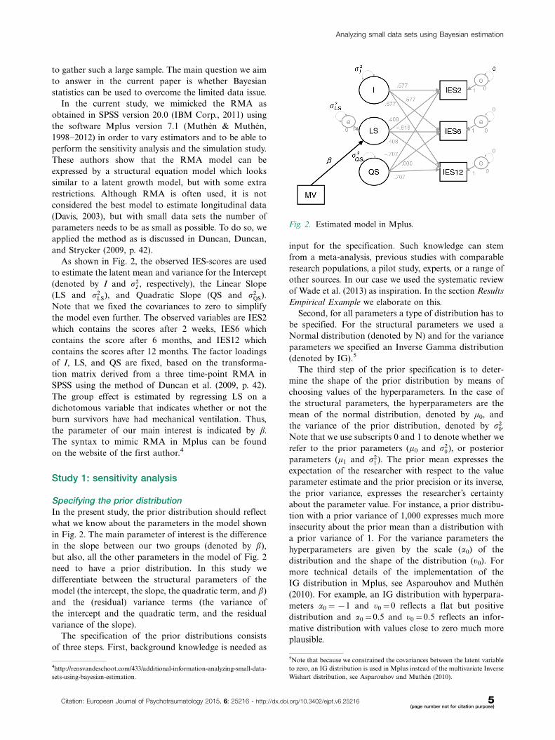
As shown in Fig. 2, the observed IES-scores are used

to estimate the latent mean and variance for the Intercept

(denoted by I and r2I , respectively), the Linear Slope

(LS and r2LS), and Quadratic Slope (QS and r2

QS).

Note that we fixed the covariances to zero to simplify

the model even further. The observed variables are IES2

which contains the scores after 2 weeks, IES6 which

contains the score after 6 months, and IES12 which

contains the scores after 12 months. The factor loadings

of I, LS, and QS are fixed, based on the transforma-

tion matrix derived from a three time-point RMA in

SPSS using the method of Duncan et al. (2009, p. 42).

The group effect is estimated by regressing LS on a

dichotomous variable that indicates whether or not the

burn survivors have had mechanical ventilation. Thus,

the parameter of our main interest is indicated by b.

The syntax to mimic RMA in Mplus can be found

on the website of the first author.4

Study 1: sensitivity analysis

Specifying the prior distributionIn the present study, the prior distribution should reflect

what we know about the parameters in the model shown

in Fig. 2. The main parameter of interest is the difference

in the slope between our two groups (denoted by b),

but also, all the other parameters in the model of Fig. 2

need to have a prior distribution. In this study we

differentiate between the structural parameters of the

model (the intercept, the slope, the quadratic term, and b)

and the (residual) variance terms (the variance of

the intercept and the quadratic term, and the residual

variance of the slope).

The specification of the prior distributions consists

of three steps. First, background knowledge is needed as

input for the specification. Such knowledge can stem

from a meta-analysis, previous studies with comparable

research populations, a pilot study, experts, or a range of

other sources. In our case we used the systematic review

of Wade et al. (2013) as inspiration. In the section Results

Empirical Example we elaborate on this.

Second, for all parameters a type of distribution has to

be specified. For the structural parameters we used a

Normal distribution (denoted by N) and for the variance

parameters we specified an Inverse Gamma distribution

(denoted by IG).5

The third step of the prior specification is to deter-

mine the shape of the prior distribution by means of

choosing values of the hyperparameters. In the case of

the structural parameters, the hyperparameters are the

mean of the normal distribution, denoted by m0, and

the variance of the prior distribution, denoted by r20.

Note that we use subscripts 0 and 1 to denote whether we

refer to the prior parameters (m0 and r20), or posterior

parameters (m1 and r21). The prior mean expresses the

expectation of the researcher with respect to the value

parameter estimate and the prior precision or its inverse,

the prior variance, expresses the researcher’s certainty

about the parameter value. For instance, a prior distribu-

tion with a prior variance of 1,000 expresses much more

insecurity about the prior mean than a distribution with

a prior variance of 1. For the variance parameters the

hyperparameters are given by the scale (a0) of the

distribution and the shape of the distribution (y0). For

more technical details of the implementation of the

IG distribution in Mplus, see Asparouhov and Muthen

(2010). For example, an IG distribution with hyperpara-

meters a0��1 and y0�0 reflects a flat but positive

distribution and a0�0.5 and y0�0.5 reflects an infor-

mative distribution with values close to zero much more

plausible.



Fig. 2. Estimated model in Mplus.

5Note that because we constrained the covariances between the latent variable

to zero, an IG distribution is used in Mplus instead of the multivariate Inverse

Wishart distribution, see Asparouhov and Muthen (2010).







In what follows, we discuss in great detail how we speci-

fied the specific hyperparameters for our PTSS-example

and we investigate by means of a sensitivity analysis what

influence the hyperparameters have on the results.

Default prior settingsAs discussed in the previous section, Bayesian estima-

tion requires prior distributions for every parameter.

First, the default settings of Mplus were used for the

prior distributions (Asparouhov & Muthen, 2010). The

default settings for the structural parameters are normal

distributions with a prior mean of zero (m0�0) and a very

large prior variance resulting in an almost flat prior

distribution (i.e., r20 �1010). These priors indicate not

much is known about the structural parameters of

the model. So, if no background knowledge would be

available, the default settings of Mplus could be used. For

the variance parameters by default an Inverse Gamma

distribution is used in Mplus with a0��1 and y0�0.

These settings result in a flat but positive distribution,

thereby making negative (residual) variances impossible,

but no information is included about the shape of the

distribution.

A fixed number of 10,000 iterations was used, and to

check convergence we increased the number of itera-

tions to 50,000 and 100,000 iterations. There appeared to

be hardly any difference for b (max �0.33 and �0.80%,

respectively). To decrease computational time we used

10,000 iterations for the remainder of our study.

The results of the analyses using ML and Bayesian

estimation relying on the default prior settings are shown

in Table 1. Only some very small numerical differences

were obtained between the coefficients of ML and

Bayesian estimation with default prior settings, but we

consider these differences as ignorable.

Informative priorsIn order to make use of the advantages of the Bayesian

toolbox, the prior distributions have to be more informa-

tive than the default settings of Mplus. To investigate

the influence of the prior specifications on the posterior

results we performed a sensitivity analysis. First, we used

a well-specified prior mean but varied the prior variance.

Next, we varied the prior mean and the prior variance.

Note that the priors should be based on background

knowledge. In the section Results Empirical Example we

actually use background information to specify the prior

distributions. For the current section we aim to investi-

gate how prior settings influence the results and therefore

we examine a wide range of different prior specifications.

Sensitivity analysis

Different values for the prior variance

In the first sensitivity analyses, a well-specified prior

mean was used for b (m0�10). That means that the prior

mean is similar as for the ML-output. In this way, the

a priori specified means are completely compatible with

the data. Note that in Bayesian analysis, priors are

by definition specified independent of the data to be

analyzed. The goal of this part of our study is to show the

performance of Bayesian analyses when only the prior

variance is varied. In the next section, we investigate

misspecification of the prior mean.

To investigate the influence of the prior variance on the

posterior results we ran a sensitivity analysis with several

values for the prior variance of b. Default prior settings

were used for the other parameters in the model. We

started with the ML results followed by the default prior

settings (r20 �1010). Then, we decreased the prior var-

iance in several steps. A prior variance of r20 �100 can

still be considered non-informative, but a prior variance

of r20 �0.1 might be considered highly informative,

maybe even too informative. However, see Van de Schoot

et al. (2013) where such highly informative priors were

used in the context of testing for measurement invariance.

In our study, however, this is not the case.

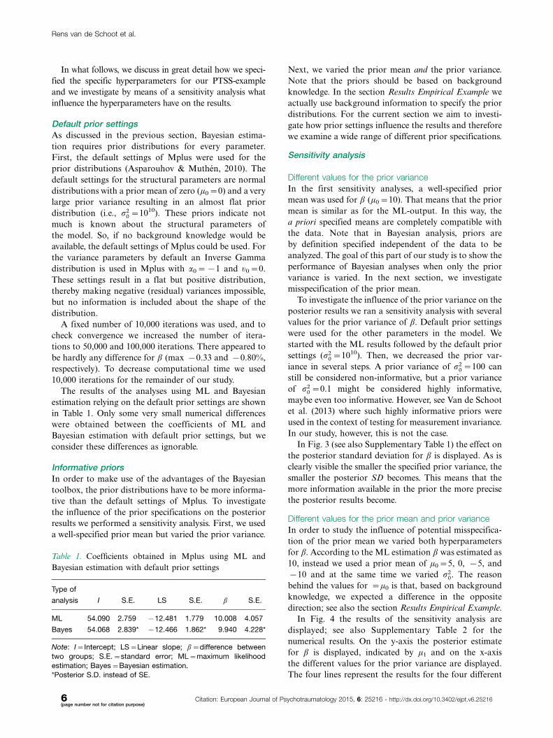
In Fig. 3 (see also Supplementary Table 1) the effect on

the posterior standard deviation for b is displayed. As is

clearly visible the smaller the specified prior variance, the

smaller the posterior SD becomes. This means that the

more information available in the prior the more precise

the posterior results become.

Different values for the prior mean and prior variance

In order to study the influence of potential misspecifica-

tion of the prior mean we varied both hyperparameters

for b. According to the ML estimation b was estimated as

10, instead we used a prior mean of m0�5, 0, �5, and

�10 and at the same time we varied r20. The reason

behind the values for �m0 is that, based on background

knowledge, we expected a difference in the opposite

direction; see also the section Results Empirical Example.

In Fig. 4 the results of the sensitivity analysis are

displayed; see also Supplementary Table 2 for the

numerical results. On the y-axis the posterior estimate

for b is displayed, indicated by m1 and on the x-axis

the different values for the prior variance are displayed.

The four lines represent the results for the four different

Table 1. Coefficients obtained in Mplus using ML and

Bayesian estimation with default prior settings

Type of

analysis I S.E. LS S.E. b S.E.

ML 54.090 2.759 �12.481 1.779 10.008 4.057

Bayes 54.068 2.839* �12.466 1.862* 9.940 4.228*

Note: I�Intercept; LS�Linear slope; b�difference between

two groups; S.E.�standard error; ML�maximum likelihood

estimation; Bayes�Bayesian estimation.*Posterior S.D. instead of SE.








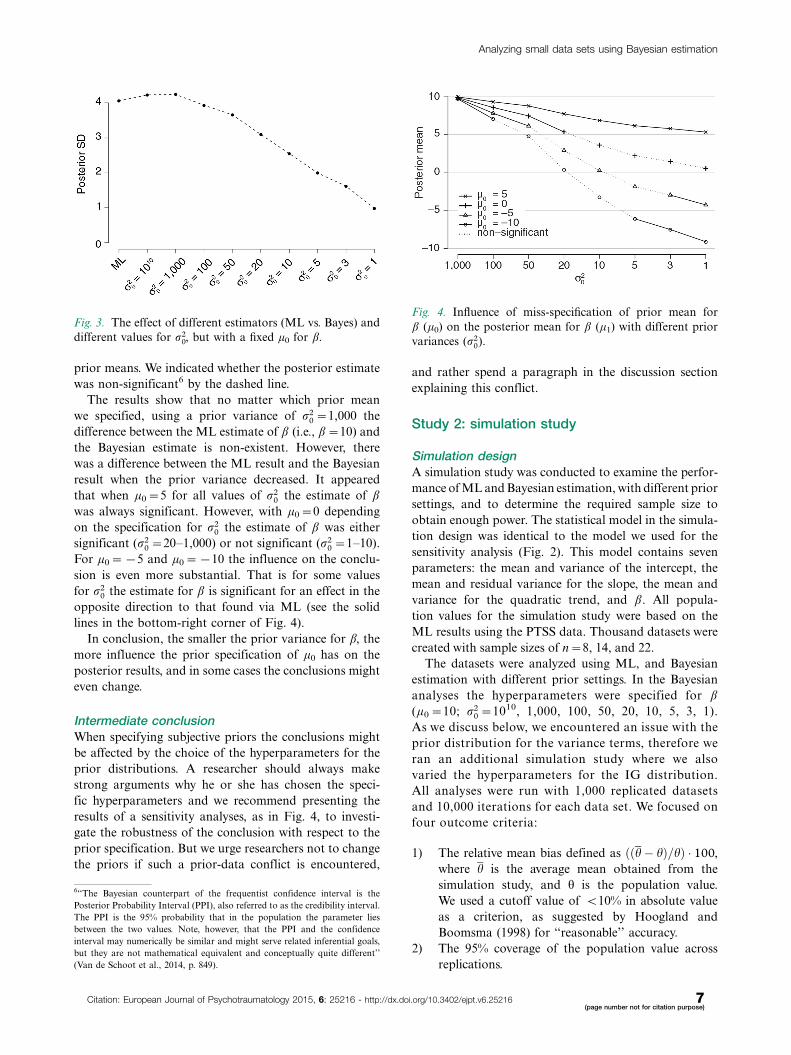
prior means. We indicated whether the posterior estimate

was non-significant6 by the dashed line.

The results show that no matter which prior mean

we specified, using a prior variance of r20 �1,000 the

difference between the ML estimate of b (i.e., b�10) and

the Bayesian estimate is non-existent. However, there

was a difference between the ML result and the Bayesian

result when the prior variance decreased. It appeared

that when m0�5 for all values of r20 the estimate of b

was always significant. However, with m0�0 depending

on the specification for r20 the estimate of b was either

significant (r20 �20�1,000) or not significant (r2

0 �1�10).

For m0��5 and m0��10 the influence on the conclu-

sion is even more substantial. That is for some values

for r20 the estimate for b is significant for an effect in the

opposite direction to that found via ML (see the solid

lines in the bottom-right corner of Fig. 4).

In conclusion, the smaller the prior variance for b, the

more influence the prior specification of m0 has on the

posterior results, and in some cases the conclusions might

even change.

Intermediate conclusionWhen specifying subjective priors the conclusions might

be affected by the choice of the hyperparameters for the

prior distributions. A researcher should always make

strong arguments why he or she has chosen the speci-

fic hyperparameters and we recommend presenting the

results of a sensitivity analyses, as in Fig. 4, to investi-

gate the robustness of the conclusion with respect to the

prior specification. But we urge researchers not to change

the priors if such a prior-data conflict is encountered,

and rather spend a paragraph in the discussion section

explaining this conflict.

Study 2: simulation study

Simulation designA simulation study was conducted to examine the perfor-

mance of ML and Bayesian estimation, with different prior

settings, and to determine the required sample size to

obtain enough power. The statistical model in the simula-

tion design was identical to the model we used for the

sensitivity analysis (Fig. 2). This model contains seven

parameters: the mean and variance of the intercept, the

mean and residual variance for the slope, the mean and

variance for the quadratic trend, and b. All popula-

tion values for the simulation study were based on the

ML results using the PTSS data. Thousand datasets were

created with sample sizes of n�8, 14, and 22.

The datasets were analyzed using ML, and Bayesian

estimation with different prior settings. In the Bayesian

analyses the hyperparameters were specified for b

(m0�10; r20 �1010, 1,000, 100, 50, 20, 10, 5, 3, 1).

As we discuss below, we encountered an issue with the

prior distribution for the variance terms, therefore we

ran an additional simulation study where we also

varied the hyperparameters for the IG distribution.

All analyses were run with 1,000 replicated datasets

and 10,000 iterations for each data set. We focused on

four outcome criteria:

1) The relative mean bias defined as ððh� hÞ=hÞ � 100,

where h is the average mean obtained from the

simulation study, and u is the population value.

We used a cutoff value of B10% in absolute value

as a criterion, as suggested by Hoogland and

Boomsma (1998) for ‘‘reasonable’’ accuracy.

2) The 95% coverage of the population value across

replications.

Fig. 3. The effect of different estimators (ML vs. Bayes) and

different values for r20, but with a fixed m0 for b.

Fig. 4. Influence of miss-specification of prior mean for

b (m0) on the posterior mean for b (m1) with different prior

variances (r20).

6‘‘The Bayesian counterpart of the frequentist confidence interval is the

Posterior Probability Interval (PPI), also referred to as the credibility interval.

The PPI is the 95% probability that in the population the parameter lies

between the two values. Note, however, that the PPI and the confidence

interval may numerically be similar and might serve related inferential goals,

but they are not mathematical equivalent and conceptually quite different’’

(Van de Schoot et al., 2014, p. 849).





3) The percentage of significance results across replica-

tion of the specific parameter as an indication of the

power.

4) The mean square error (MSE).

Simulation results

Results for maximum likelihood

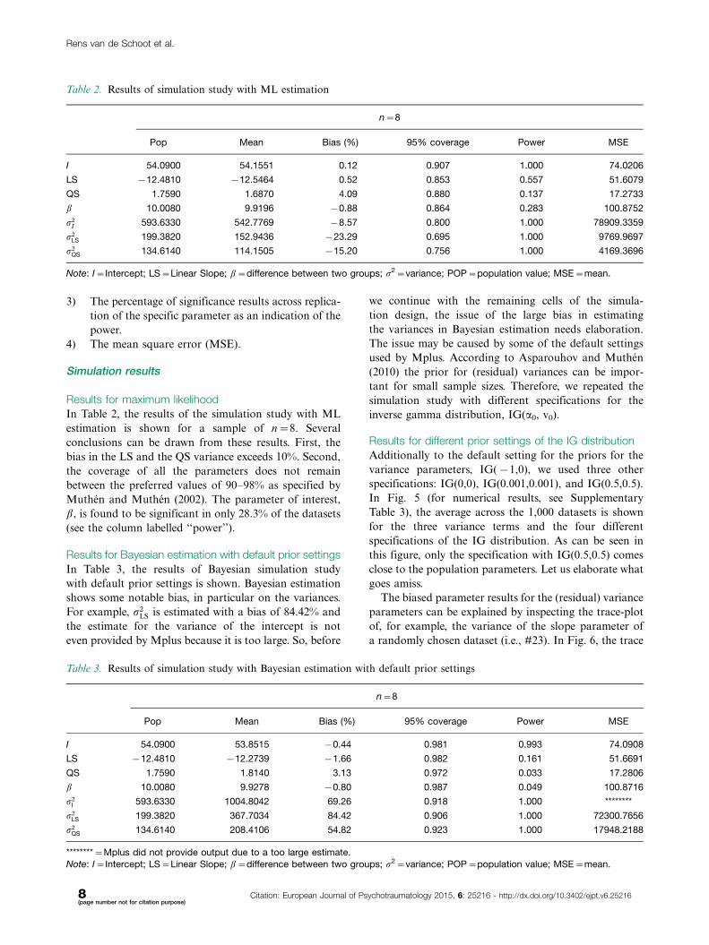
In Table 2, the results of the simulation study with ML

estimation is shown for a sample of n�8. Several

conclusions can be drawn from these results. First, the

bias in the LS and the QS variance exceeds 10%. Second,

the coverage of all the parameters does not remain

between the preferred values of 90�98% as specified by

Muthen and Muthen (2002). The parameter of interest,

b, is found to be significant in only 28.3% of the datasets

(see the column labelled ‘‘power’’).

Results for Bayesian estimation with default prior settings

In Table 3, the results of Bayesian simulation study

with default prior settings is shown. Bayesian estimation

shows some notable bias, in particular on the variances.

For example, r2LS is estimated with a bias of 84.42% and

the estimate for the variance of the intercept is not

even provided by Mplus because it is too large. So, before

we continue with the remaining cells of the simula-

tion design, the issue of the large bias in estimating

the variances in Bayesian estimation needs elaboration.

The issue may be caused by some of the default settings

used by Mplus. According to Asparouhov and Muthen

(2010) the prior for (residual) variances can be impor-

tant for small sample sizes. Therefore, we repeated the

simulation study with different specifications for the

inverse gamma distribution, IG(a0, v0).

Results for different prior settings of the IG distribution

Additionally to the default setting for the priors for the

variance parameters, IG(�1,0), we used three other

specifications: IG(0,0), IG(0.001,0.001), and IG(0.5,0.5).

In Fig. 5 (for numerical results, see Supplementary

Table 3), the average across the 1,000 datasets is shown

for the three variance terms and the four different

specifications of the IG distribution. As can be seen in

this figure, only the specification with IG(0.5,0.5) comes

close to the population parameters. Let us elaborate what

goes amiss.

The biased parameter results for the (residual) variance

parameters can be explained by inspecting the trace-plot

of, for example, the variance of the slope parameter of

a randomly chosen dataset (i.e., #23). In Fig. 6, the trace

Table 2. Results of simulation study with ML estimation

n�8

Pop Mean Bias (%) 95% coverage Power MSE

I 54.0900 54.1551 0.12 0.907 1.000 74.0206

LS �12.4810 �12.5464 0.52 0.853 0.557 51.6079

QS 1.7590 1.6870 4.09 0.880 0.137 17.2733

b 10.0080 9.9196 �0.88 0.864 0.283 100.8752

r2I 593.6330 542.7769 �8.57 0.800 1.000 78909.3359

r2LS 199.3820 152.9436 �23.29 0.695 1.000 9769.9697

r2QS 134.6140 114.1505 �15.20 0.756 1.000 4169.3696

Note: I�Intercept; LS�Linear Slope; b�difference between two groups; s2�variance; POP�population value; MSE�mean.

Table 3. Results of simulation study with Bayesian estimation with default prior settings

n�8


I 54.0900 53.8515 �0.44 0.981 0.993 74.0908

LS �12.4810 �12.2739 �1.66 0.982 0.161 51.6691

QS 1.7590 1.8140 3.13 0.972 0.033 17.2806

b 10.0080 9.9278 �0.80 0.987 0.049 100.8716

r2I 593.6330 1004.8042 69.26 0.918 1.000 ********

r2LS 199.3820 367.7034 84.42 0.906 1.000 72300.7656

r2QS 134.6140 208.4106 54.82 0.923 1.000 17948.2188

********�Mplus did not provide output due to a too large estimate.Note: I�Intercept; LS�Linear Slope; b�difference between two groups; s2�variance; POP�population value; MSE�mean.








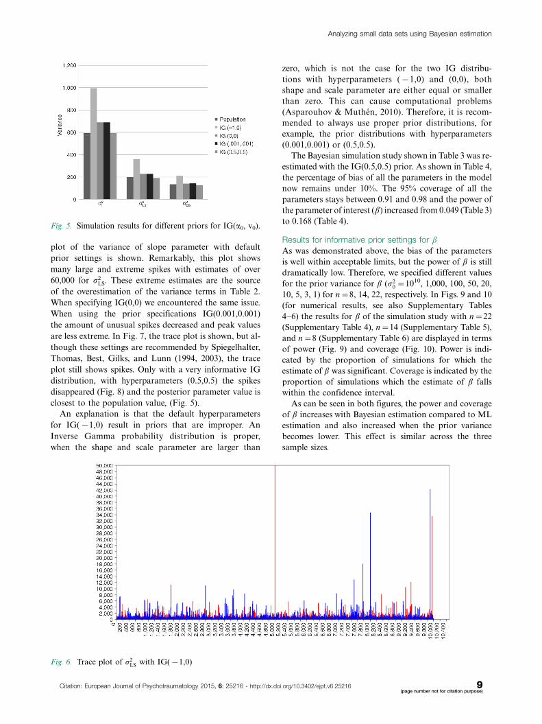
plot of the variance of slope parameter with default

prior settings is shown. Remarkably, this plot shows

many large and extreme spikes with estimates of over

60,000 for r2LS. These extreme estimates are the source

of the overestimation of the variance terms in Table 2.

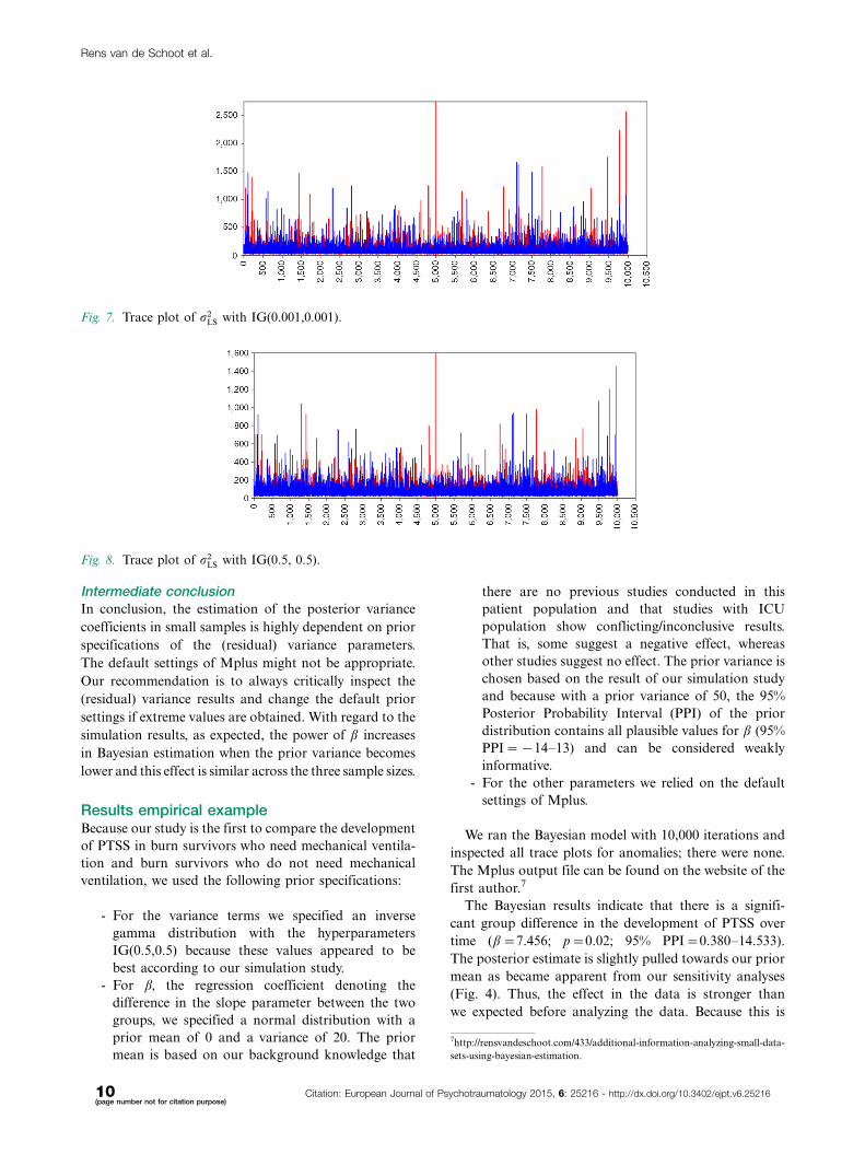
When specifying IG(0,0) we encountered the same issue.

When using the prior specifications IG(0.001,0.001)

the amount of unusual spikes decreased and peak values

are less extreme. In Fig. 7, the trace plot is shown, but al-

though these settings are recommended by Spiegelhalter,

Thomas, Best, Gilks, and Lunn (1994, 2003), the trace

plot still shows spikes. Only with a very informative IG

distribution, with hyperparameters (0.5,0.5) the spikes

disappeared (Fig. 8) and the posterior parameter value is

closest to the population value, (Fig. 5).

An explanation is that the default hyperparameters

for IG(�1,0) result in priors that are improper. An

Inverse Gamma probability distribution is proper,

when the shape and scale parameter are larger than

zero, which is not the case for the two IG distribu-

tions with hyperparameters (�1,0) and (0,0), both

shape and scale parameter are either equal or smaller

than zero. This can cause computational problems

(Asparouhov & Muthen, 2010). Therefore, it is recom-

mended to always use proper prior distributions, for

example, the prior distributions with hyperparameters

(0.001,0.001) or (0.5,0.5).

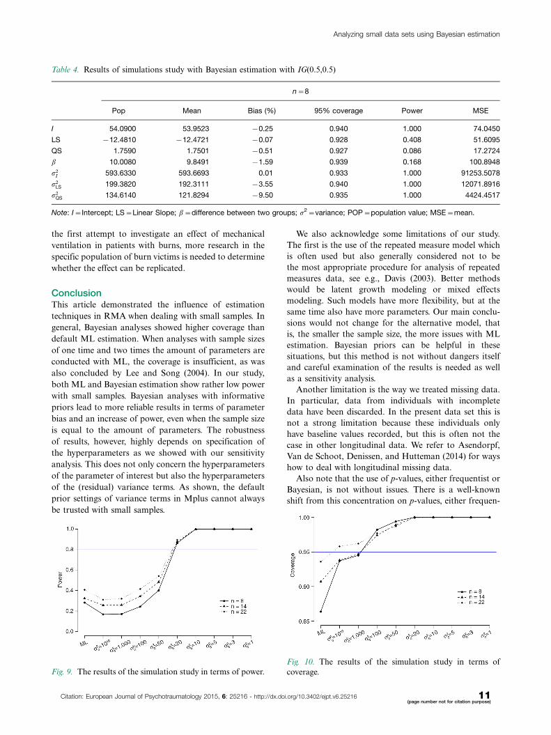
The Bayesian simulation study shown in Table 3 was re-

estimated with the IG(0.5,0.5) prior. As shown in Table 4,

the percentage of bias of all the parameters in the model

now remains under 10%. The 95% coverage of all the

parameters stays between 0.91 and 0.98 and the power of

the parameter of interest (b) increased from 0.049 (Table 3)

to 0.168 (Table 4).

Results for informative prior settings for b

As was demonstrated above, the bias of the parameters

is well within acceptable limits, but the power of b is still

dramatically low. Therefore, we specified different values

for the prior variance for b (r20 �1010, 1,000, 100, 50, 20,

10, 5, 3, 1) for n�8, 14, 22, respectively. In Figs. 9 and 10

(for numerical results, see also Supplementary Tables

4�6) the results for b of the simulation study with n�22

(Supplementary Table 4), n�14 (Supplementary Table 5),

and n�8 (Supplementary Table 6) are displayed in terms

of power (Fig. 9) and coverage (Fig. 10). Power is indi-

cated by the proportion of simulations for which the

estimate of b was significant. Coverage is indicated by the

proportion of simulations which the estimate of b falls

within the confidence interval.

As can be seen in both figures, the power and coverage

of b increases with Bayesian estimation compared to ML

estimation and also increased when the prior variance

becomes lower. This effect is similar across the three

sample sizes.

Fig. 5. Simulation results for different priors for IG(a0, v0).

Fig. 6. Trace plot of r2LS with IG(�1,0)
















Intermediate conclusionIn conclusion, the estimation of the posterior variance

coefficients in small samples is highly dependent on prior

specifications of the (residual) variance parameters.

The default settings of Mplus might not be appropriate.

Our recommendation is to always critically inspect the

(residual) variance results and change the default prior

settings if extreme values are obtained. With regard to the

simulation results, as expected, the power of b increases

in Bayesian estimation when the prior variance becomes

lower and this effect is similar across the three sample sizes.

Results empirical exampleBecause our study is the first to compare the development

of PTSS in burn survivors who need mechanical ventila-

tion and burn survivors who do not need mechanical

ventilation, we used the following prior specifications:

- For the variance terms we specified an inverse

gamma distribution with the hyperparameters

IG(0.5,0.5) because these values appeared to be

best according to our simulation study.

- For b, the regression coefficient denoting the

difference in the slope parameter between the two

groups, we specified a normal distribution with a

prior mean of 0 and a variance of 20. The prior

mean is based on our background knowledge that

there are no previous studies conducted in this

patient population and that studies with ICU

population show conflicting/inconclusive results.

That is, some suggest a negative effect, whereas

other studies suggest no effect. The prior variance is

chosen based on the result of our simulation study

and because with a prior variance of 50, the 95%

Posterior Probability Interval (PPI) of the prior

distribution contains all plausible values for b (95%

PPI��14�13) and can be considered weakly

informative.

- For the other parameters we relied on the default

settings of Mplus.

We ran the Bayesian model with 10,000 iterations and

inspected all trace plots for anomalies; there were none.

The Mplus output file can be found on the website of the

first author.7

The Bayesian results indicate that there is a signifi-

cant group difference in the development of PTSS over

time (b�7.456; p�0.02; 95% PPI�0.380�14.533).

The posterior estimate is slightly pulled towards our prior

mean as became apparent from our sensitivity analyses

(Fig. 4). Thus, the effect in the data is stronger than

we expected before analyzing the data. Because this is

Fig. 8. Trace plot of r2LS with IG(0.5, 0.5).



Fig. 7. Trace plot of r2LS with IG(0.001,0.001).








the first attempt to investigate an effect of mechanical

ventilation in patients with burns, more research in the

specific population of burn victims is needed to determine

whether the effect can be replicated.

ConclusionThis article demonstrated the influence of estimation

techniques in RMA when dealing with small samples. In

general, Bayesian analyses showed higher coverage than

default ML estimation. When analyses with sample sizes

of one time and two times the amount of parameters are

conducted with ML, the coverage is insufficient, as was

also concluded by Lee and Song (2004). In our study,

both ML and Bayesian estimation show rather low power

with small samples. Bayesian analyses with informative

priors lead to more reliable results in terms of parameter

bias and an increase of power, even when the sample size

is equal to the amount of parameters. The robustness

of results, however, highly depends on specification of

the hyperparameters as we showed with our sensitivity

analysis. This does not only concern the hyperparameters

of the parameter of interest but also the hyperparameters

of the (residual) variance terms. As shown, the default

prior settings of variance terms in Mplus cannot always

be trusted with small samples.

We also acknowledge some limitations of our study.

The first is the use of the repeated measure model which

is often used but also generally considered not to be

the most appropriate procedure for analysis of repeated

measures data, see e.g., Davis (2003). Better methods

would be latent growth modeling or mixed effects

modeling. Such models have more flexibility, but at the

same time also have more parameters. Our main conclu-

sions would not change for the alternative model, that

is, the smaller the sample size, the more issues with ML

estimation. Bayesian priors can be helpful in these

situations, but this method is not without dangers itself

and careful examination of the results is needed as well

as a sensitivity analysis.

Another limitation is the way we treated missing data.

In particular, data from individuals with incomplete

data have been discarded. In the present data set this is

not a strong limitation because these individuals only

have baseline values recorded, but this is often not the

case in other longitudinal data. We refer to Asendorpf,

Van de Schoot, Denissen, and Hutteman (2014) for ways

how to deal with longitudinal missing data.

Also note that the use of p-values, either frequentist or

Bayesian, is not without issues. There is a well-known

shift from this concentration on p-values, either frequen-

Table 4. Results of simulations study with Bayesian estimation with IG(0.5,0.5)

n�8


I 54.0900 53.9523 �0.25 0.940 1.000 74.0450

LS �12.4810 �12.4721 �0.07 0.928 0.408 51.6095

QS 1.7590 1.7501 �0.51 0.927 0.086 17.2724

b 10.0080 9.8491 �1.59 0.939 0.168 100.8948

r2I 593.6330 593.6693 0.01 0.933 1.000 91253.5078

r2LS 199.3820 192.3111 �3.55 0.940 1.000 12071.8916

r2QS 134.6140 121.8294 �9.50 0.935 1.000 4424.4517

Note: I�Intercept; LS�Linear Slope; b�difference between two groups; s2�variance; POP�population value; MSE�mean.

Fig. 9. The results of the simulation study in terms of power.Fig. 10. The results of the simulation study in terms of

coverage.





tist or Bayesian, toward more emphasis on estimated

relationships, confidence (or credibility) intervals, clinical

relevance, and replication (see Asendorpf et al., 2013).

A final remark concerns the dependence on prior speci-

fications in Bayesian estimation, which, might be seen

as controversial, because of their subjective nature. It

requires expert knowledge about the use of prior spe-

cifications and the research topic. Statistical analyses are

usually connected with objectivity, but Bayesian estima-

tion brings in a more subjective element. If and how prior

knowledge can be incorporated raises philosophical

issues. Nevertheless, a small research population, like

burn survivors but also multicenter studies, could benefit

from the techniques described in this paper.

From a practical point of view, we advise ML or

objective Bayesian estimation when the sample size is

equal to or larger than three times the amount of

parameters. Although Bayesian estimation provides reli-

able results when sample sizes are small, power can remain

an issue. When prior information is available, subjec-

tive priors can offer the opportunity for research on

small research populations to increase accuracy, coverage,

and power. But such analyses should always be accom-

panied by a sensitivity analyses to investigate the influence

of the specification of the hyperparameters of the prior

distribution.

Conflict of interest and funding

Funding for this study was provided by a grant from The

Netherlands Organization for Scientific Research: NWO-

VENI-451-11-008. The original study was financially

supported by the Dutch Burns Foundation.

References

American Psychiatric Association. (2013). Diagnostic and statistical

manual of mental disorders (5th ed.). Washington, DC: Author.

Asendorpf, J. B., Conner, M., De Fruyt, F., De Houwer, J.,

Denissen, J. J. A., Fiedler, K., et al. (2013). Recommendations

for increasing replicability in psychology. European Journal of

Personality, 27, 108�119. doi: 10.1002/per.1919.

Asendorpf, J. B., Van de Schoot, R., Denissen, J. J. A., & Hutteman, R.

(2014). Reducing bias due to systematic attrition in longitudinal

studies: The benefits of multiple imputation. International Journal

of Behaviroural Development, 38(5), 453�460.

Asparouhov, T., & Muthen, B. (2010). Bayesian analysis of latent

variable models using Mplus. Retrieved June 17, 2014, from

http://www.statmodel2.com/download/BayesAdvantages18.pdf.

Baldi, E., Liuzzo, A., & Bucherelli, C. (2013). Fimbria-fornix

and entorhinal cortex differential contribution to contextual

and cued fear conditioning consolidation in rats. Physiology &

Behavior, 114�115, 42�48.

Belgian Outcome in Burn Injury Study Group (2009). Development

and validation of a model for prediction of mortality in

patients with acute burn injury. The British journal of surgery,

96, 111�117.

Breslau, N., Kessler, R. C., Chilcoat, H. D., Schultz, L. R., Davis,

G. C., & Andreski, P. (1998). Trauma and posttraumatic stress

disorder in the community: The 1996 Detroit area survey of

trauma. Archives of General Psychiatry, 55(7), 626�632.

Brom, D., & Kleber, R. J. (1985). De Schok Verwerkings Lijst

[Shock Processing List]. Nederlands Tijdschrift voor de

Psychologie, 40, 164�168.

Button, K. S., Ioannidis, J. P., Mokrysz, C., Nosek, B. A., Flint, J.,

Robinson, E. S., et al. (2013). Power failure: Why small sample

size undermines the reliability of neuroscience. Nature Reviews

Neuroscience, 14(5), 365�376.

Datta, S., & O’Malley, M. W. (2013). Fear extinction memory

consolidation requires potentiation of pontine-wave activity

during REM sleep. The Journal of Neuroscience, 33(10),

4561�4569.

Davis, C. (2003). Statistical methods for the analysis of repeated

measurements. New York: Springer-Verlag.

Depaoli, S. (2012). Measurement and structural model class separation

in mixture CFA: ML/EM versus MCMC. Structural Equation

Modeling, 178�203.

Duncan, T., Duncan, S., & Strycker, L. (2009). An introduction to

latent variable growth curve modeling: Concepts, issues and

applications (2nd ed.). Mahwah, NJ: Lawrence Erlbaum.

Galindo-Garre, F., Vermunt, J. K., & Bregsma, W. P. (2004).

Bayesian posterior estimation of logit parameters with small

samples. Sociological Methods & Research, 33(1), 88�117.

Gelman, A., Carlin, J., Stern, H., & Rubin, D. (2004). Bayesian data

analysis (2nd ed.). London: Chapman & Hall.

Hoogland, J. J., & Boomsma, A. (1998). Robustness studies

in covariance structure modeling. Sociological Methods &

Research, 26(3), 329�368.

Horowitz, M., Wilner, N., & Alvarez, W. (1979). Impact of event

scale: A measure of subjective stress. Psychosomatic Medicine,

41(3), 209�218.

Hox, J., Moerbeek, M., Kluytmans, A., Van De Schoot, R. (2014).

Analyzing indirect effects in cluster randomized trials. The

effect of estimation method, number of groups and group sizes

on accuracy and power. Frontiers in psychology, 5, 78. doi:

10.3389/fpsyg.2014.00078.

Hox, J., Van de Schoot, R., & Matthijsse, S. (2012). How few

countries will do? Comparative survey analysis from a

Bayesian perspective. Survey Research Methods, 6, 87�93.

IBM Corp. (2011). IBM SPSS Statistics for Windows, Version 20.0.

Armonk, NY: Author.

Jackman, S. (2009). Bayesian analysis for the social sciences.

Chichester, UK: Wiley.

Kaplan, D., & Depaoli, S. (2012). Bayesian structural equation

modeling. In R. Hoyle (Ed.), Handbook of structural equation

modeling (pp. 650�673). New York: Guilford.

Kruschke, J. K., Aguinis, H., & Joo, H. (2012). The time has come:

Bayesian methods for data analysis in the organizational

sciences. Organizational Research Methods, 15(4), 722�752.

Lee, S.-Y., & Song, X.-Y. (2004). Evaluation of the Bayesian and

maximum likelihood approaches in analyzing structural equa-

tion models with small sample sizes. Multivariate Behavioral

Research, 39(4), 653�686.

Mies van der Rohe, L. (1994). The presence of Mies (D. Mertins,

Ed.). New York: Princeton Architectural Press.

Muthen, L. K., & Muthen, B. O. (1998�2012). Mplus user’s guide

(7th ed.). Los Angeles, CA: Muthen & Muthen.

Muthen, L. K., & Muthen, B. O. (2002). How to use a Monte Carlo

study to decide on sample size and determine power. Structural

Equation Modeling, 9(4), 599�620.

Parsons, R. G., & Ressler, K. J. (2013). Implications of memory

modulation for post-traumatic stress and fear disorders.

Nature Neuroscience, 16(2), 146�153.

Peto, R., Pike, M. C., Armitage, P., Breslow, N. E., Cox, D. R.,

Howard, S. V., et al. (1976). Design and analysis of randomized




http://www.statmodel2.com/download/BayesAdvantages18.pdf



clinical trials requiring prolonged observation of each patient.

I. Introduction and design. British Journal of Cancer, 34(6),

585�612.

Price, L. R. (2012). Small sample properties of Bayesian multivariate

autoregressive time series models. Structural Equation Model-

ing: A Multidisciplinary Journal, 19(1), 51�64.

Schafe, G. E., Nader, K., Blair, H. T., & LeDoux, J. E. (2001).

Memory consolidation of Pavlovian fear conditioning: A

cellular and molecular perspective. TRENDS in Neurosciences,

24(9), 540�546.

Scheines, R., Hoijtink, H., & Boomsma, A. (1999). Bayesian estima-

tion and testing of structural equation models. Psychometrika,

64(1), 37�52.

Spiegelhalter, D., Thomas, A., Best, N., Gilks, W., & Lunn, D.

(1994, 2003). BUGS: Bayesian inference using Gibbs sampling.

Cambridge, UK: MRC Biostatistics Unit. Retrieved from

http://www.mrc-bsu.cam.ac.uk/bugs

Van de Schoot, R., Kaplan, D., Denissen, J., Asendorpf, J. B., Neyer,

F. J., & Van Aken, M. A. (2014). A gentle introduction to

Bayesian analysis: Applications to research in child develop-

ment. Child Development, 85, 842�860.

Van de Schoot, R., Kluytmans, A., Tummers, L., Lugtig, P., Hox, J.,

& Muthen, B. (2013). Facing off with Scylla and Charybdis:

A comparison of scalar, partial, and the novel possibility of

approximate measurement invariance. Frontiers in Psychology,

4, 770. doi: 10.3389/fpsyg.2013.00770.

Van Loey, N. E., Maas, C. J., Faber, A. W., & Taal, L. A. (2003).

Predictors of chronic posttraumatic stress symptoms following

burn injury: Results of a longitudinal study. Journal of

Traumatic Stress, 16(4), 361�369.

Van Loey, N., Van Beeck, E., Faber, A., Van de Schoot, R., &

Bremer, M. (2012). Health-related quality of life after burns:

A prospective multicentre cohort study with 18 months follow-

up. Journal of Trauma and Acute Care Surgery, 72(2), 513�520.

doi: 10.1097/TA.0b013e3182199072.

Van Loey, N., & Van Son, M. J. M. (2003). Psychopathology and

psychological problems in patients with burn scars: Epide-

miology and management. American Journal of Clinical

Dermatology, 4, 245�272.

Wade, D., Hardy, R., Howell, D., & Mythen, M. (2013). Identifying

clinical and acute psychological risk factors for PTSD after

critical care: A systematic review. Minerva Anestesiologica, 79,

1�20.

Wigg, D. (2012). ‘For me, it’s the bigger the better . . . in everything’:

BBC documentary goes behind the scenes with the late, great

Freddie Mercury. Retrieved June 17, 2014, from http://www.

dailymail.co.uk/tvshowbiz/article-2216408/BBC-documentary-

goes-scens-late-great-Freddie-Mercury.html

Zohar, J., Juven-Wetzler, A., Myers, V., & Fostick, L. (2008). Post-

traumatic stress disorder: Facts and fiction. Current Opinion in

Psychiatry, 21(1), 74�77.

Zyphur, M., & Oswald, F. (2015). Bayesian estimation and

inference: A user’s guide. Journal of Management, 41(2),

390�420.



http://www.mrc-bsu.cam.ac.uk/bugs

http://www.dailymail.co.uk/tvshowbiz/article-2216408/BBC-documentary-goes-scens-late-great-Freddie-Mercury.html





Documents

EUROPEAN JOURNAL OF PSYCHOTRAUMATOLOGY