European Shadow Banking and Money Demand

by

Luís Miguel Pereira de Moura

Master Dissertation in Economics

Faculdade de Economia, Universidade do Porto

Supervised by:

José Peres Jorge

September, 2016

i

Biographic note

Luís Moura was born in 1993, in the town of Póvoa de Varzim. In this town he

progressed through his early educational career, finishing both his basic and secondary

phase as a member of the excellency board, while a member of the local basketball

team.

Graduated with a bachelor‟s degree in 2014, three years after entering the

Faculty of Economics of Oporto (FEP). Was accepted into the Masters Program in

Economics following the summer break and now presents the corresponding

dissertation, while engaging in voluntary work with his local Rotaract Club.

ii

Acknowledgments

I would like to thank first all the teachers that accompanied me during this

climb. Their dedication and commitment to present students with a massive amount of

knowledge, required in the modern world, is an altruistic act in its nature that allowed

me to be in this position. More recently, José Peres Jorge gave his time to counsel both

me and four other students during this stressful phase, for which I am thankful. Also,

Natércia Fortuna showed a constant availability to aid in any and every question

regarding the econometric section of the work, with the same “get-up-and-go” attitude

and politeness I had got used to during her pleasant, yet tough, classes.

Friends have their constant role holding me up during life and in times like these

their presence is greatly noticed and appreciated. They know who they are. Four other

students helped me during this stage as they also went through it: Sara Gonçalves, João

Cerqueira, Daniela Silva and Andreia Coelho. I wish I had met you under less eventful

times.

Finally, I have to thank my family as they had to endure me through this phase,

at the same time as they faced hardships of their own. Sadly, they cannot avoid me (or

me them), so the only thing left is to hold this boat together. I‟m sure I wouldn‟t wish it

any other way. Thank you.

iii

Resumo

Esta dissertação visa verificar, seguindo os mesmos processos apresentados por

Sunderam (2015), se as operações de recompra, o activo de curto-prazo mais usado pela

banca sombra como fonte de financiamento, oferecem serviços monetários; isto é, têm

liquidez e segurança suficientes para poderem servir como reserva de valor. Analisando

o período entre julho de 2001 e agosto de 2008, é possível encontrar sinais positivos de

que tal se verifica, embora não seja possível apresentar uma resposta definitiva.

Códigos-JEL: E41, E44, G23

Palavras-chave: banca sombra, repo, oferta monetária, serviços monetários

iv

Abstract

Following the same procedures presented in Sunderam (2015), I test whether

repos, the most common short-term source of financing used by the European Shadow

Banking Sector, offered money-like services. The predictions provided by his model

present favourable empirical results in the euro area.

JEL-codes: E41, E44, G23

Key-words: shadow banking, repurchase agreements, money-like services,

money supply

v

Contents

Biographic note ............................................................................................................... i

Acknowledgments .........................................................................................................ii

Resumo ........................................................................................................................ iii

Abstract ......................................................................................................................... iv

List of tables .................................................................................................................. vi

List of figures ...............................................................................................................vii

Introduction .................................................................................................................... 1

Chapter 1. Sunderam‟s Model ....................................................................................... 4

1.1. Households and Demand ...................................................................................... 4

1.2. Supply of Claims .................................................................................................. 6

1.3. Predictions ............................................................................................................ 7

Chapter 2. Data, Models and Results ........................................................................... 10

2.1. Data .................................................................................................................... 10

2.2. Models and Results ............................................................................................ 11

2.2.1. Prediction 1: Low yields on Treasury bills should forecast an increase of repo

activity by the Shadow Banking System ............................................................ 11

2.2.2. Prediction 4: Low Treasury bills should forecast increases in the supply of reserves

by the Central Bank ............................................................................................ 14

2.2.3. Prediction 5: The interbank funding rate should be high when Treasury bill yields

are low, unless the rate is perfectly stabilized .................................................... 15

2.2.4. Testing the Treasury bill yield OIS gap as a proxy for money demand ............ 17

Conclusions .................................................................................................................. 19

References .................................................................................................................... 21

vi

List of tables

Table 1 – Summary Statistics ......................................................................................... 10

Table 2 – Results for the First Prediction ....................................................................... 13

Table 3 – Results for the Fourth Prediction .................................................................... 15

Table 4 – Results for the Fifth Prediction ....................................................................... 16

Table 5 – Results for the regression with the money aggregates .................................... 18

vii

List of figures

Figure 1 – Balance Sheet Composition ............................................................................. 6

Figure 2 – Evolution of Repo ......................................................................................... 12

Figure 3 – Evolution of the Spread between the German 3 Month Yield and the 3 Month

Overnight Indexed Swap ................................................................................................ 12

Figure 4 – Evolution of Reserves ................................................................................... 14

Figure 5 – Evolution of the “European Central Bank Spread” ....................................... 16

Figure 6 – Evolution of the money aggregates ............................................................... 17

1

Introduction

Does the European Shadow Banking‟s short term debt offer money services?

Following the procedures presented by Sunderam (2015), I test if the author‟s

conclusions are also valid for the euro area, by checking if shadow banking debt

behaves as a substitute for other claims that are safe, liquid and able to store value

effectively: government debt bills and bank deposits.

The Shadow Banking system “consists of a web of specialized financial

institutions that conduct credit, maturity and liquidity transformation without direct,

explicit access to public backstops” (Adrian and Ashcraft, 2012, 10). According to

Bouveret (2011), repurchase agreements (repo) were the dominant instrument used by

this system to fund itself, surpassing Asset-backed Commercial Paper (ABCP) in the

euro area. They are the “type of transaction in which a money market participant

acquires immediately available funds by selling securities and simultaneously agreeing

to repurchase the same or similar securities after a specified time at a given price, which

typically includes interest at an agreed-upon rate. Such a transaction is called repo when

viewed from the perspective of the supplier of the securities (the party acquiring funds)

and a reverse repo or matched sale-purchase agreement when described from the point

of view of the supplier of funds” (Lumpkin, 1998, 59). While it would be easier to keep

using ABCP like Sunderam, replacing it with repo brings the analysis closer to the

European reality. This work is the first to simultaneously use this analysis on this

economic area and to focus on repo rather than ABCP, despite the challenges obtaining

data.

Sunderam‟s model generates five predictions that he later confronts with the

US„s data. After the relevant adaptations to the euro area, they are the following:

1- Low yields on Treasury bills should forecast an increase of repo activity by

the Shadow Banking System: high demand for Treasury bills should make

substitutes also more attractive.

2- Treasury bill issuance and repo activity should be negatively correlated:

increasing the quantity of an asset crowds out the demand for its substitutes.

2

3- Shorter maturity repo should respond more strongly to Treasury bill yields:

they should be safer and more liquid and thus be a closer substitute to

Treasury bills.

4- Low Treasury bill yields should forecast increases in the supply of reserves

by the Central Bank: the increasing money demand will impact deposits

demand, which in turn require reserves. To keep the rate at its target, new

reserves need to be injected to counter the increased demand.

5- The interbank funding rate should be high when Treasury bill yields are low,

unless the rate is perfectly stabilized: the increased demand for deposits will

drive banks‟ demand for reserves in the interbank market, raising prices.

These predictions stem from the fact that T-bills, deposits and repo all provide

money services and are imperfect substitutes of one another. Thus, the demand for

money-like claim is linked with the remaining claims.

The dataset starts at July, 2001 and ends at August 2008, running in a monthly

frequency. The EONIA, MRO rates and outstanding repo time series were obtained at

the ECB; Thomson Reuters provided the time series for the Overnight Indexed Swaps,

German 3 Month Yields and mandatory reserves at the central bank. The predictions

were verified statistically, connecting the growth of money-like claims with the growth

of repurchase agreements and deposits, leaving only Treasury bills unchecked.

Literature Review The literature on Shadow Banking focuses on the factors

that explain its development and growth. These factors can be grouped into three

categories: “innovation in the composition of aggregate money supply, capital, tax and

accounting arbitrage and finally, other agency problems in financial markets” (Adrian

and Ashcraft, 2012, 10).

Firstly, the “innovation in the composition of aggregate money supply” category

considers the possibility of shadow banking short-term liabilities being able to offer

“money services”: being considered safe and liquid enough to be used as a store of

value (Sunderam, 2015). My work fits into this category. Since liquidity is a pre-

requisite for supplying money services, this field touches the literature on liquidity, such

as Holmström and Tirole (1998). If Shadow Banking Debt provides money-like services

(which include liquidity), it will be part of the private suppliers of liquid claims. If this

3

sector increases in size, then liquidity shocks will be more severe and demand greater

efforts by the public sector to cover for private supply‟s shortcomings.

Secondly, the “capital, tax and accounting arbitrage” category focuses on the

role of regulation and policymaking as catalysts for the growth of the Shadow Banking

sector. Friedman (2009) considers that the sector developed as a response to an over-

complicated web of regulations that fostered securitization activities. Acemoglu (2009)

in turn believes that regulations were insufficient or ineffective. Levitin and Wachter

(2012) defend the shift from regulated securitization to unregulated securitization as the

main factor behind the severity of the American Housing Bubble of 2004-2007.

Acharya, Schnabl and Suarez (2013) link the changes made to regulatory capital rules to

the rapid growth of ABCP activity, which was used to finance American Shadow

Banking activity.

Finally, the “other agency problems in financial markets” category highlights

information asymmetry issues in the securitization market, along its value chain. In

particular, Ashcraft and Schuermann (2008) describe the issues between the several

agents in the market, namely lenders, originators, investors, servicers, borrowers,

beneficiaries of invested funds, asset managers and credit rating agencies. Another

interesting perspective is provided by Mathis, McAndrews and Rochet (2009): given the

reliance on ratings provided by Credit Rating Agencies, is their reputation alone

sufficient to discipline the agencies themselves? Errors in their evaluation affect the

entire system and conflicting interests are known to exist.

The literature on the topic is still in its infancy and focuses on the American

crisis and the housing bubble that preceded it. In Europe, Bakk-Simon et al. (2012)

provide an extensive overview of Shadow Banking in Europe. However, the literature

focusing on the euro area is thin; this work intends to provide a humble step in that

direction.

4

Chapter 1. Sunderam’s Model

Sunderam‟s (2015) model admits three categories of agents, all risk neutral for

simplicity: households (including firms), banks (both traditional sector and shadow

sector) and the monetary authority.

1.1 . Households and Demand

Households demand money-like services: safety, liquidity, a store of value and,

in the case of deposits, transaction services. Sunderam (2015) admits three types of

claims that can provide any of the money-like services previously mentioned: deposits,

Treasury bills and Asset Backed Commercial Paper (ABCP). However, he also admits

that each of the claims provides different amounts of those services, due to their

different nature. The quantity provided by deposits for each monetary unit invested is

normalized to 1 ( ), while the quantity provided by the other claims ( and ) is

lower but still positive

.

Households try to maximize the effective amount of money-like services given

by these claims together, taking into consideration the amount invested into each one. It

is assumed that the elasticity of substitution between them is constant. This results in

the following equation:

(

)

,

where M is the total money-like services provided to households,

are the amounts of deposits, Treasury bills and ABCP (respectively) expressed in

monetary units and is the elasticity of substitution between deposits, Treasury Bills

and ABCP. In accordance to Krishnamurthy and Vissing-Jorgensen (2012), Sunderam

5

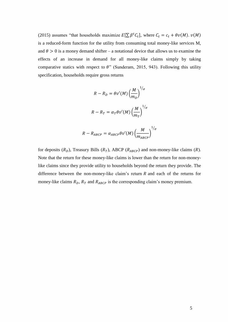
(2015) assumes “that households maximize [∑ ], where ( ). ( )

is a reduced-form function for the utility from consuming total money-like services M,

and is a money demand shifter – a notational device that allows us to examine the

effects of an increase in demand for all money-like claims simply by taking

comparative statics with respect to ” (Sunderam, 2015, 943). Following this utility

specification, households require gross returns

( ) (

)

⁄

( ) (

)

⁄

( ) (

)

⁄

for deposits ( ), Treasury Bills ( ), ABCP ( ) and non-money-like claims ( ).

Note that the return for these money-like claims is lower than the return for non-money-

like claims since they provide utility to households beyond the return they provide. The

difference between the non-money-like claim‟s return and each of the returns for

money-like claims , and is the corresponding claim‟s money premium.

6

1.2 . Supply of claims

Looking now at the supply of claims, they are produced by the government

(Treasury bills) and by banks (deposits and ABCP). Sunderam (2015) assumes that the

supply of Treasury bills is exogenous, that there is a continuum of banks of size one and

that they take the aggregate supply of money-like services and prices of the claims as

given. Banks can have two categories of assets: reserves, which provide no return, and

projects, which are expected to return F>R. Their liabilities can be long-term bonds,

Deposits and ABCP, which serve as their external sources of financing. Due to the

small weight of capital, it is excluded from the figure. In the short run, banks are

assumed to be unable to expand their balance sheets, so they can simply change the

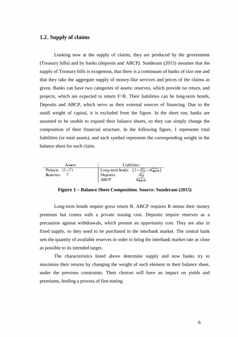
composition of their financial structure. In the following figure, 1 represents total

liabilities (or total assets), and each symbol represents the corresponding weight in the

balance sheet for each claim.

Figure 1 – Balance Sheet Composition. Source: Sunderam (2015)

Long-term bonds require gross return R. ABCP requires R minus their money

premium but comes with a private issuing cost. Deposits require reserves as a

precaution against withdrawals, which present an opportunity cost. They are also in

fixed supply, so they need to be purchased in the interbank market. The central bank

sets the quantity of available reserves in order to bring the interbank market rate as close

as possible to its intended target.

The characteristics listed above determine supply and now banks try to

maximize their returns by changing the weight of each element in their balance sheet,

under the previous constraints. Their choices will have an impact on yields and

premiums, feeding a process of fine-tuning.

7

1.3 . Predictions

After describing the model and its agents, the relevant conclusions that it

provides will now be summarized, expressing the expected behavior in the data. These

are all presented by Sunderam (2015); I merely list them here and present the

adaptations necessary to the new economic environment. These changes result from

different reference rates (since the responsible institution is now the European Central

Bank instead of the Federal Reserve) and from the predominant use of a different

instrument by the European Shadow Banking, repo. Both represent short-term loans

with requiring, by definition, collateral and their markets were widely used to fund the

Shadow Banking sector, though their importance varies geographically. When

considering repo activity, the work excludes

The author assumes two sources of exogenous variation: variation in overall

money demand and in the supply of Treasury Bills. The predictions generated are the

following:

Prediction 1: Low yields (high prices) on Treasury bills should forecast an

increase of repo activity by the Shadow Banking system.

An increase in money demand results in high prices for money-like services,

which in the model consist in Treasury bills, deposits and repo. The high demand thus

lowers yields for Treasury bills. To respond to higher money demand, the banking

system will be interested in offering more repo, to capture the higher money premium,

or in other words, capture the higher discount in return required by households, in

comparison to non-money-like claims. Offering more repo will lower costs for banks.

Prediction 2: Treasury bill issuance and repo activity should be negatively

correlated.

Since Treasury bills and repo are imperfect substitutes, issuing more of either of

them will crowd out the demand for the other. Another way to explain this prediction is

to look at Prediction 1: if Treasury bill issuance is increased, prices will decrease,

8

reducing the repo money premium available to be captured. Therefore, banks save less

on costs by offering more repo. Increased Treasury bill issuance “crowded out” repo

activity.

Prediction 3: Shorter maturity repo should respond more strongly to

Treasury bill yields.

Shorter maturity repo should provide more money-like services than longer term

repo. As a result, the first will be a closer substitute to Treasury bills and thus react

more strongly to changes in their yields.

Prediction 4: Low Treasury bill yields should forecast increases in the

supply of reserves by the Central Bank.

If Treasury bill yields are low, their price is high. As a result, household demand

will drift to the other two money-like claims, deposits and repo. The increased amount

of deposits will require the bank to buy additional reserves in the interbank market,

driving the rate upwards. The central bank will increase the supply of reserves in order

to push the rate back to its target.

Prediction 5: The interbank funding rate should be high when Treasury bill

yields are low, unless the rate is perfectly stabilized.

When investors are highly interested in liquidity, government bills, deposits and

shadow bank debt should also be in high demand. Increased demand for deposits

increases the demand for reserves leading to an increase in the interbank rate for

reserves. In the model, the dynamic does not apply if the rate is perfectly stabilized,

though in reality, exogenous shocks make such result practically impossible to obtain.

9

These conclusions describe the expected behaviour if these assets are substitutes

in the “money-like” claims market1. The following step is to take these predictions and

face them against the available data.

1 Sunderam (2015) also considers the possibility that at high frequencies, writing repo contracts, simply

cover banks‟ need for financing at high frequencies. In that case, since they do not provide money-like

services, no linkages should arise between these markets and the markets for Treasury bills and reserves.

Under this possibility, verifying the predictions with the data will not yield any results. Obtaining

statistically significant linkages rules out this possibility.

10

Chapter 2. Data, Models and Results

2.1. Data

The time series used span from July, 2001 until August, 2008, at a monthly

frequency2. In order to obtain as many observations as possible, the time period under

analysis ends in the month before the Lehman Brothers bankruptcy.

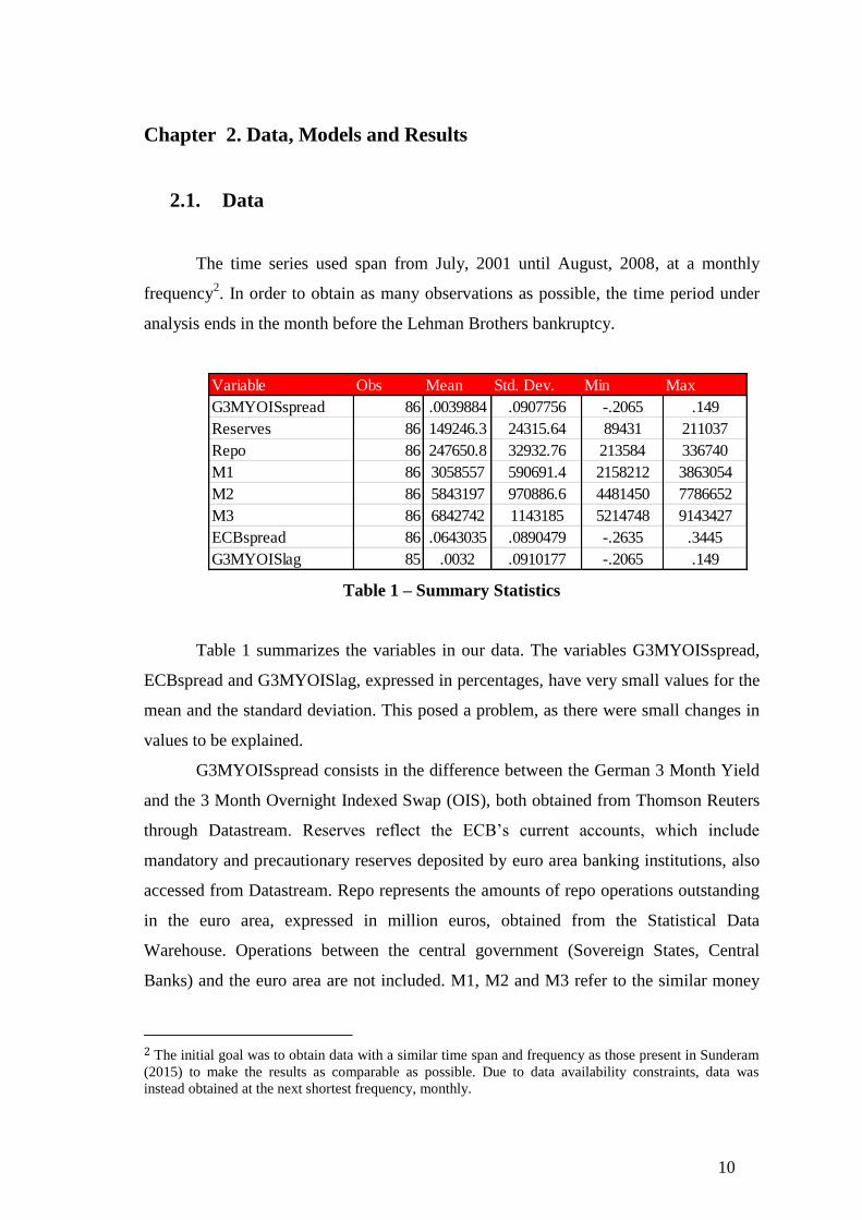
Table 1 – Summary Statistics

Table 1 summarizes the variables in our data. The variables G3MYOISspread,

ECBspread and G3MYOISlag, expressed in percentages, have very small values for the

mean and the standard deviation. This posed a problem, as there were small changes in

values to be explained.

G3MYOISspread consists in the difference between the German 3 Month Yield

and the 3 Month Overnight Indexed Swap (OIS), both obtained from Thomson Reuters

through Datastream. Reserves reflect the ECB‟s current accounts, which include

mandatory and precautionary reserves deposited by euro area banking institutions, also

accessed from Datastream. Repo represents the amounts of repo operations outstanding

in the euro area, expressed in million euros, obtained from the Statistical Data

Warehouse. Operations between the central government (Sovereign States, Central

Banks) and the euro area are not included. M1, M2 and M3 refer to the similar money

2 The initial goal was to obtain data with a similar time span and frequency as those present in Sunderam

(2015) to make the results as comparable as possible. Due to data availability constraints, data was

instead obtained at the next shortest frequency, monthly.

Variable Obs Mean Std. Dev. Min Max

G3MYOISspread 86 .0039884 .0907756 -.2065 .149

Reserves 86 149246.3 24315.64 89431 211037

Repo 86 247650.8 32932.76 213584 336740

M1 86 3058557 590691.4 2158212 3863054

M2 86 5843197 970886.6 4481450 7786652

M3 86 6842742 1143185 5214748 9143427

ECBspread 86 .0643035 .0890479 -.2635 .3445

G3MYOISlag 85 .0032 .0910177 -.2065 .149

11

aggregates. ECBspread is the difference between the EONIA and the Main Refinancing

Operations rate, obtained at the ECB‟s Statistical Data Warehouse (SDW).

The G3MYOISspread variable provides a proxy for the yield for money-like

services. The German 3 Month yield incorporates the effects of short-term interest rates,

as well as credit risk and liquidity premia. Overnight Indexed Swaps “carry little risk

and are a good proxy for risk-free rates purged of liquidity and credit risk premia”

(Brunnermeier, 2009; Duffie and Choudhry, 2011; Feldhutter and Lando, 2008; Gorton

and Metrick, 2010a; Schwarz, 2010; in Sunderam, 2015, 953). The OIS thus serves as

an indictation of the overall level of short-term interest rates. Using the spread between

Treasury bills and OIS “essentially strips out variation in the Treasury bill yield driven

by changes in the overall level of short-term interest rates” (Sunderam, 2015, 953) thus

capturing the information about the money premium that is embedded in Treasury bill

yields.

2.2. Models and Results

The work now tests the predictions 1-5 presented previously, accompanied by

the corresponding model used for each prediction.

2.2.1. Prediction 1: Low yields on Treasury bills should forecast

an increase of repo activity by the Shadow Banking

System.

In order to test this prediction, the following model was estimated:

( ) ( )

Repo is a time series with the outstanding amounts of repurchase agreements in

the euro area for period t. G3MYOISlag is equal to the G3MYOISspread but lagged one

period. Ln represents the natural logarithm, and are the coefficients to be estimated

and the error terms.

12

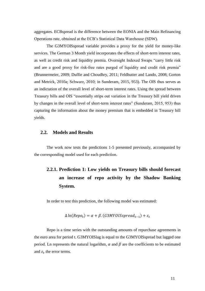
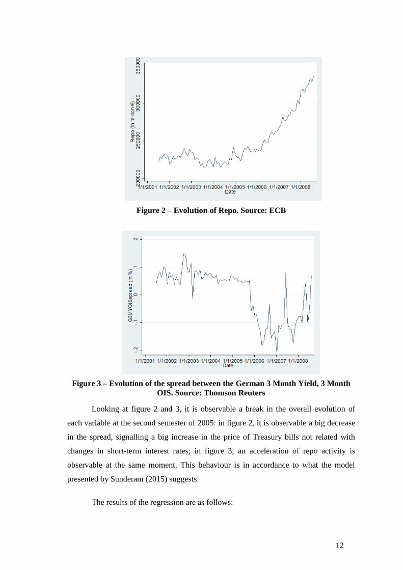
Figure 2 – Evolution of Repo. Source: ECB

Figure 3 – Evolution of the spread between the German 3 Month Yield, 3 Month

OIS. Source: Thomson Reuters

Looking at figure 2 and 3, it is observable a break in the overall evolution of

each variable at the second semester of 2005: in figure 2, it is observable a big decrease

in the spread, signalling a big increase in the price of Treasury bills not related with

changes in short-term interest rates; in figure 3, an acceleration of repo activity is

observable at the same moment. This behaviour is in accordance to what the model

presented by Sunderam (2015) suggests.

The results of the regression are as follows:

13

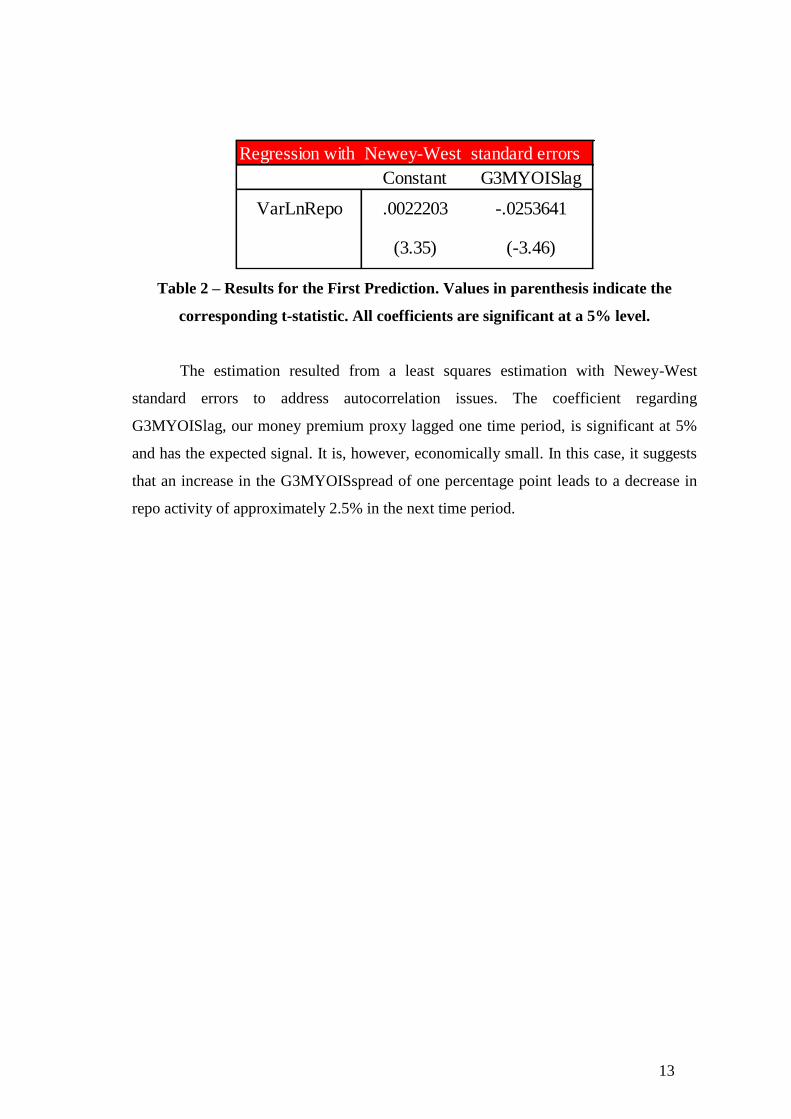
Table 2 – Results for the First Prediction. Values in parenthesis indicate the

corresponding t-statistic. All coefficients are significant at a 5% level.

The estimation resulted from a least squares estimation with Newey-West

standard errors to address autocorrelation issues. The coefficient regarding

G3MYOISlag, our money premium proxy lagged one time period, is significant at 5%

and has the expected signal. It is, however, economically small. In this case, it suggests

that an increase in the G3MYOISspread of one percentage point leads to a decrease in

repo activity of approximately 2.5% in the next time period.

Regression with Newey-West standard errors

Constant G3MYOISlag

VarLnRepo .0022203 -.0253641

(3.35) (-3.46)

14

2.2.2. Prediction 4: Low Treasury bill yields should forecast

increases in the supply of reserves by the Central Bank.

The following expression will be used to put the prediction to the test:

( ) ( )

Reserves are given by a time series with the ECB‟s current accounts, which in

turn contains mandatory and precautionary reserves from banks in the Eurosystem, held

by the central bank.

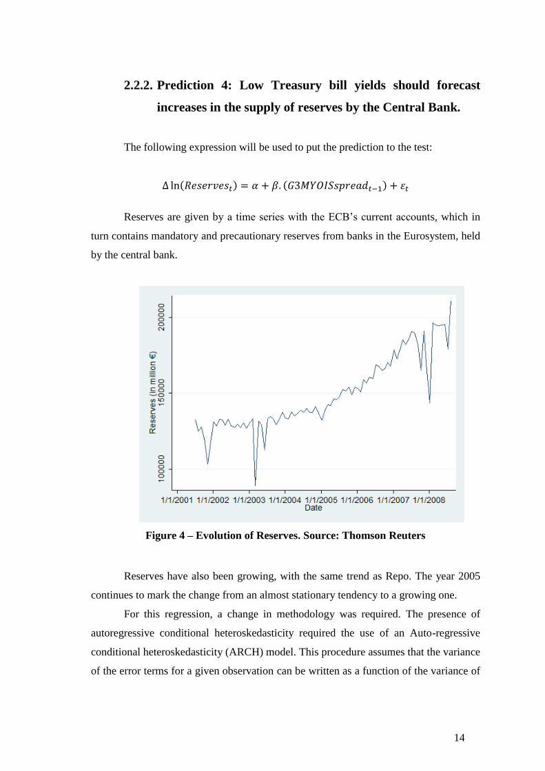
Figure 4 – Evolution of Reserves. Source: Thomson Reuters

Reserves have also been growing, with the same trend as Repo. The year 2005

continues to mark the change from an almost stationary tendency to a growing one.

For this regression, a change in methodology was required. The presence of

autoregressive conditional heteroskedasticity required the use of an Auto-regressive

conditional heteroskedasticity (ARCH) model. This procedure assumes that the variance

of the error terms for a given observation can be written as a function of the variance of

15

the error terms of previous observations, plus white noise. More information can be

found on manuals such as Asteriou and Hall (2011).

For the following test, the variance for each observation is given by a function

containing the variance of the immediately previous one, ARCH (1).

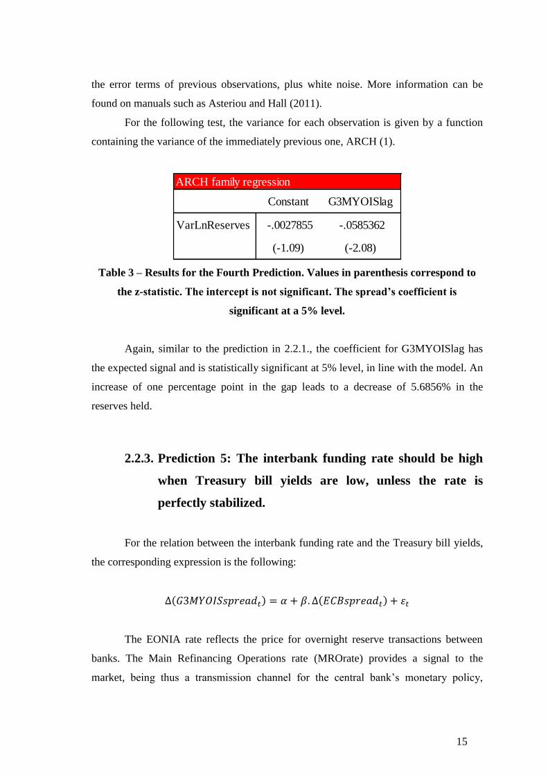
Table 3 – Results for the Fourth Prediction. Values in parenthesis correspond to

the z-statistic. The intercept is not significant. The spread’s coefficient is

significant at a 5% level.

Again, similar to the prediction in 2.2.1., the coefficient for G3MYOISlag has

the expected signal and is statistically significant at 5% level, in line with the model. An

increase of one percentage point in the gap leads to a decrease of 5.6856% in the

reserves held.

2.2.3. Prediction 5: The interbank funding rate should be high

when Treasury bill yields are low, unless the rate is

perfectly stabilized.

For the relation between the interbank funding rate and the Treasury bill yields,

the corresponding expression is the following:

( ) ( )

The EONIA rate reflects the price for overnight reserve transactions between

banks. The Main Refinancing Operations rate (MROrate) provides a signal to the

market, being thus a transmission channel for the central bank‟s monetary policy,

ARCH family regression

Constant G3MYOISlag

VarLnReserves -.0027855 -.0585362

(-1.09) (-2.08)

16

according to the ECB (2011). The difference between the two results is what is labelled

as the ECBspread.

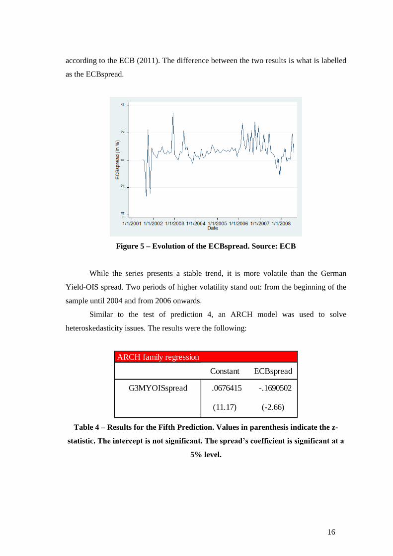
Figure 5 – Evolution of the ECBspread. Source: ECB

While the series presents a stable trend, it is more volatile than the German

Yield-OIS spread. Two periods of higher volatility stand out: from the beginning of the

sample until 2004 and from 2006 onwards.

Similar to the test of prediction 4, an ARCH model was used to solve

heteroskedasticity issues. The results were the following:

Table 4 – Results for the Fifth Prediction. Values in parenthesis indicate the z-

statistic. The intercept is not significant. The spread’s coefficient is significant at a

5% level.

ARCH family regression

Constant ECBspread

G3MYOISspread .0676415 -.1690502

(11.17) (-2.66)

17

Again, the results are statistically significant at a 5% level and the relationship

between the variables has the expected signal: as Treasury bill yields decrease, the

interbank market rate increases, after taking into account the effects of short-term rates

and central bank injection rate.

2.2.4. Testing the Treasury bill yield OIS spread as a proxy for

money demand

As a final step, I test the German Yield-OIS gap as a tool to detect money

demand shocks, following the procedure done by Sunderam (2015). If it truly behaves

in accordance to money demand, “increases in demand should raise prices and

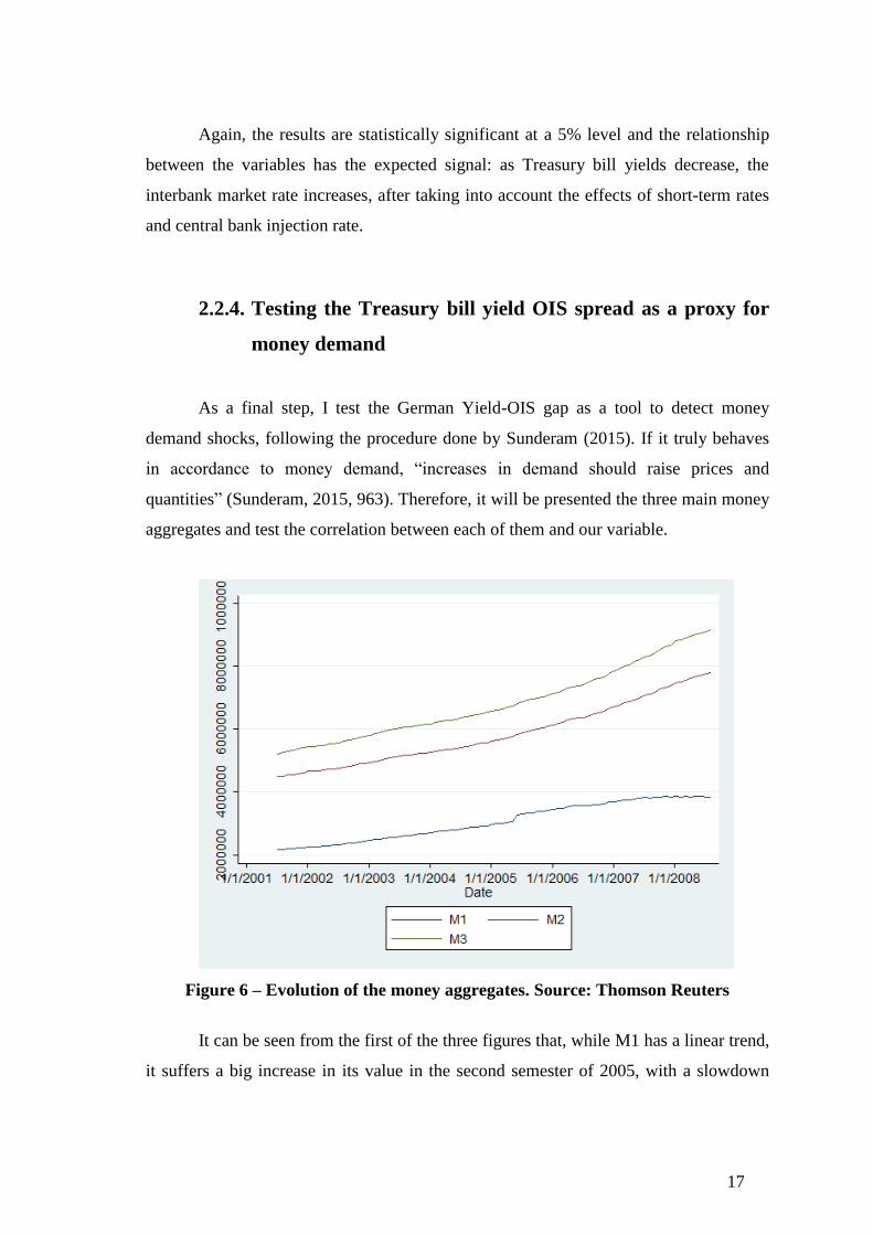
quantities” (Sunderam, 2015, 963). Therefore, it will be presented the three main money

aggregates and test the correlation between each of them and our variable.

Figure 6 – Evolution of the money aggregates. Source: Thomson Reuters

It can be seen from the first of the three figures that, while M1 has a linear trend,

it suffers a big increase in its value in the second semester of 2005, with a slowdown

18

from 2007 onwards. The other two aggregates, M2 and M3, present an increase in the

pace of their growth from the second half of 2005, although a far more subtle one.

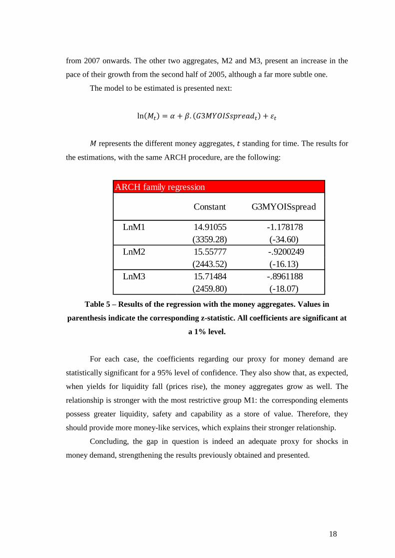
The model to be estimated is presented next:

( ) ( )

represents the different money aggregates, standing for time. The results for

the estimations, with the same ARCH procedure, are the following:

Table 5 – Results of the regression with the money aggregates. Values in

parenthesis indicate the corresponding z-statistic. All coefficients are significant at

a 1% level.

For each case, the coefficients regarding our proxy for money demand are

statistically significant for a 95% level of confidence. They also show that, as expected,

when yields for liquidity fall (prices rise), the money aggregates grow as well. The

relationship is stronger with the most restrictive group M1: the corresponding elements

possess greater liquidity, safety and capability as a store of value. Therefore, they

should provide more money-like services, which explains their stronger relationship.

Concluding, the gap in question is indeed an adequate proxy for shocks in

money demand, strengthening the results previously obtained and presented.

ARCH family regression

Constant G3MYOISspread

LnM1 14.91055 -1.178178

(3359.28) (-34.60)

LnM2 15.55777 -.9200249

(2443.52) (-16.13)

LnM3 15.71484 -.8961188

(2459.80) (-18.07)

19

Conclusions

This work provides evidence that shadow banking debt provides money-like

services. The end goal was to relate the growth of money demand with the growth of

shadow banking activity. While I was unable to provide enough evidence for a

definitive answer, they do provide signals that, indeed short-term shadow debt provides

money-like services, which would help explain the sector‟s pre-crisis growth.

Inspired by Sunderam (2015), I was able to test the proxy for money demand

and link it to the time series for repo activity, the predominant short-term source of

funding of this sector in the euro area. I was also able to link it to the amounts held as

reserves at the ECB, as a requirement for deposits held by banks. Finally, I confirmed

the connection between money demand with the interbank market for reserves, taking

into account the cost for new reserves issued by the central bank. These links are

statistically significant.

The first problem was the inability to link the shadow debt to treasury bills as

substitutes due to the lack of data regarding their outstanding amounts. This was also

true when trying to prove the effect of shadow debt's maturity in its capability of

providing money-like services. As a result, since these two final connections were not

tested, I cannot state irrefutably that the European Shadow Banking sector created

money-like claims and that these were the force behind their growth until the recent

crisis.

Increased availability of data would be greatly appreciated for future academic

works since it would allow new venues for investigation, as well as ease hypothesis

testing. Also, new and different model specifications could provide interesting insights:

the data for several variables suggested two different "states": prior 2005 and after. A

Structural Break model could thus provide evidence on different "states", though it

would be more interesting with a larger period to be analysed.

As Bakk-Simon et al. (2012) showed, the shadow banking activity did not fall

nearly as much in Europe as in the American case, showing even signs of a recovery.

The aim of this work was to provide insights into the expected behaviour of the Shadow

Banking activity. It would benefit monetary policy to have a better understanding of the

sector in order to improve the quality and precision of future monetary analysis and

20

interventions. It is expected that this topic will fuel more discussion and analysis in the

future which, looking at the effects of the latest crisis in the economy, will be greatly

welcomed so as to prevent similar developments in the future.

21

References

Acemoglu, D. (2009), “The Crisis of 2008: Lessons for and from Economics,

Critical Review, Vol. 21. Nº 2-3, pp. 185-194.

Acharya, V. and M. Richardson (2009), “Causes of the Financial Crisis”,

Critical Review, Vol. 21, Nº 2-3, pp. 195-210.

Acharya, V., P. Schnabl and G. Suarez (2013), “Securitization Without Risk

Transfer”, Journal of Financial Economics, Vol. 107(3), pp. 515-519.

Adrian, T. and A. Ashcraft (2012), “Shadow Banking: a Review of the

Literature”, Federal Reserve Bank of New York Staff Reports, Nº580, pp. 1-15

Ashcraft, A. and T. Schuermann (2008), “Understanding the securitization of

subprime mortgage credit”, Now Publishers Inc., Nº3.

Asteriou, D. and S. Hall (2007), “Applied Econometrics – Revised Edition”,

Palgrave Macmillan, pp. 248-276.

Bakk-Simon, K., S. Borgioli, C. Giron, H. Hempbell, A. Maddaloni, F. Recine

and S. Rosati (2012), “Shadow Banking in the Euro Area: an Overview”, ECB:

Occasional Paper Series, Nº133, pp. 1-33.

Bouveret, A. (2011), “An Assessment of Shadow Banking in Europe”, SSRN

Working Paper, NewYork: Social Science Research Network, July, pp. 1-32.

ECB (2011), “The Monetary Policy of the ECB”, European Central Bank, May,

pp. 93-105

Friedman, J. (2009), “A crisis of Policy, not Economics: Complexity, Ignorance

and Policy Failure”, Critical Review, Vol. 21, Nº 2-3, pp. 127-183.

Gorton, G. and A. Metrick (2012), “Securitized Banking and the Run on Repo”,

Journal of Financial Economics, Vol. 104, Nº3, pp. 425-451.

Holmström, B. and J. Tirole (1998), “Private and Public Supply of Liquidity”,

The Journal of Political Economy, Vol. 106, Nº1, pp. 1-6.

Levitin, A. and S. Wachter (2012), “Explaining the Housing Bubble”,

Georgetown Law Journal, Vol. 100, pp. 1177-1187.

Lumpkin, S. (1998), “Repurchase and Reverse Repurchase Agreements”,

Instruments of the Money Market, Federal Reserve Bank of Richmond, pp.59-60

22

Poznar, Z., T. Adrian, A. Ashcraft and H. Boesky (2010), “Shadow Banking”,

Federal Reserve Bank of New York Staff Reports, Nº 458, pp. 1-20

Sunderam, A. (2015), “Money Creation and the Shadow Banking System”, The

Review of Financial Studies, Vol.28, n.4, pp. 939-977.