Embed Size (px)
Citation preview

CIMAT
Evader Surveillance under Incomplete
Information
by
Israel Becerra Duran
Advisor: Dr. Rafael Murrieta Cid
A thesis submitted in partial fulfillment for the
Master’s Degree in Computer Science
in the
Computer Science Department in CIMAT
November 2010

“Where did you happen to be when I founded the earth? Tell me, if you do know under-
standing...When the morning stars joyfully cried out together, and all the sons of God
began shouting in applause?”
Job 38:4,7

CIMAT
Abstract
Computer Science Department in CIMAT
Master’s Degree in Computer Science
by Israel Becerra Duran
This work is concerned with determining whether a mobile robot, called the pursuer,
is up to maintaining visibility of an antagonist agent, called the evader. This problem,
a variant of pursuit-evasion, has been largely studied, following a systematic treatment
by increasingly relaxing a number of restrictions. In this case we deal with incomplete
information, and we say so because the pursuer only knows where the evader will be in
a small progress of time and the pursuer does not know the motion policy of the evader,
all of these under a strong mutual visibility framework ([1]).
In this thesis, we prove that there are cases for which an evader may escape only if it does
not travel the shortest path to an escapable region. We introduce planning strategies for
the movement of the pursuer that keeps track of the evader, even if the evader chooses
not to travel the shortest path to an escape region. We also present a sufficient condition
for the evader to escape that does not depend on the initial positions of the players. It
can be verified only using the environment. Experiments and simulation results about
the proposed algorithms are also presented.

Acknowledgements
First of all I want to thank Jesus Christ for being my saviour, and for filling me with
his love so that I could have a reason for living. I want to thank him because is due to
his mercy and his grace that I could successfully end this stage in my life.
I also want to thank my advisor Rafael because without his guidance this work would
not have came to light, and specially I would not be working in this research area if he
would not have introduced me to robotics research.
With no less importance, I’m really grateful to my wife who has always supported me
unconditionally and has always help me to look for God’s perfect will. My whole family,
specially my mom and my sister, has also been really important encouraging me at all
time.
Moreover, I want to thank all my partners during this stage, Nacho, Lalo, Wil, Omar
M., Moncho, Hugo, Omar G., Joaquin, Paco, Rigo, Ubaldo and Chucho. Without them
I would not have had so much fun during all this time.
Finally, I want to thank CONACyT for providing me with financial support during all
my master’s degree studies.
iii
Contents
Abstract ii
Acknowledgements iii
List of Figures vi
List of Tables vii
1 Introduction 1
1.1 Problem Definition . . . . . . . . . . . . . . . . . . . . . . . . . . . . . . . 3
1.2 Contributions . . . . . . . . . . . . . . . . . . . . . . . . . . . . . . . . . . 4
2 Related Work 5
2.1 Target Finding . . . . . . . . . . . . . . . . . . . . . . . . . . . . . . . . . 5
2.2 Target Tracking . . . . . . . . . . . . . . . . . . . . . . . . . . . . . . . . . 6
3 Strong Mutual Visibility 10
3.1 Strong Mutual Visibility . . . . . . . . . . . . . . . . . . . . . . . . . . . . 10
3.2 Environment partition . . . . . . . . . . . . . . . . . . . . . . . . . . . . . 11
3.3 Finding strongly mutually visible regions . . . . . . . . . . . . . . . . . . . 13
3.4 Two graphs modeling the environment . . . . . . . . . . . . . . . . . . . . 13
3.5 Preventing From Escape Constrain . . . . . . . . . . . . . . . . . . . . . . 14
4 The Effect of Incomplete Information Over the Paths to Escape 16
4.1 The Case of a Faster Evader . . . . . . . . . . . . . . . . . . . . . . . . . . 17
4.2 The Case of a Slower Evader . . . . . . . . . . . . . . . . . . . . . . . . . 18
5 Keeping or Escaping Pursuer surveillance 24
5.1 Players Strategies and Paths . . . . . . . . . . . . . . . . . . . . . . . . . 24
5.2 Initial Conditions . . . . . . . . . . . . . . . . . . . . . . . . . . . . . . . . 26
5.3 Combinatoric Paths . . . . . . . . . . . . . . . . . . . . . . . . . . . . . . 27
5.3.1 Ω borders . . . . . . . . . . . . . . . . . . . . . . . . . . . . . . . . 30
5.3.2 Regions of Local Solution . . . . . . . . . . . . . . . . . . . . . . . 36
6 Simulation Results 39
6.1 Paths of sequences’ type . . . . . . . . . . . . . . . . . . . . . . . . . . . . 39
iv

Contents v
6.2 Paths of cycles’ type . . . . . . . . . . . . . . . . . . . . . . . . . . . . . . 47
7 Discussion and Conclusion 49
7.1 Conclusions . . . . . . . . . . . . . . . . . . . . . . . . . . . . . . . . . . . 49
7.2 Future work . . . . . . . . . . . . . . . . . . . . . . . . . . . . . . . . . . . 50
A Reduced Visibility Graph 53
B Configuration Space 54
Bibliography 56
List of Figures
3.1 Classical visibility (obtained from [1]) . . . . . . . . . . . . . . . . . . . . 11
3.2 Environment partition and resulting graphs (obtained from [1]) . . . . . . 12
4.1 Evader faster than the pursuer . . . . . . . . . . . . . . . . . . . . . . . . 17
4.2 Evader slower than the pursuer . . . . . . . . . . . . . . . . . . . . . . . . 18
4.3 Comparison between fte (t)↔ te (RA) and ftpe (t) ↔ tpe (RA′). . . . . . 22
5.1 Paths types . . . . . . . . . . . . . . . . . . . . . . . . . . . . . . . . . . . 25
5.2 Long Term Paths . . . . . . . . . . . . . . . . . . . . . . . . . . . . . . . . 27
5.3 Inflexion rays ordering . . . . . . . . . . . . . . . . . . . . . . . . . . . . . 30
5.4 Ω borders . . . . . . . . . . . . . . . . . . . . . . . . . . . . . . . . . . . . 34
5.5 Ω borders calculation . . . . . . . . . . . . . . . . . . . . . . . . . . . . . . 35
5.6 S set example . . . . . . . . . . . . . . . . . . . . . . . . . . . . . . . . . . 38
6.1 Simulation Results – first simulation with paths of sequences’ type . . . . 40
6.2 Map with 58 reflex vertices . . . . . . . . . . . . . . . . . . . . . . . . . . 42
6.3 Simulation Results – display of big simulated map . . . . . . . . . . . . . 44
6.4 Simulation Results – big map with paths of sequences’ type . . . . . . . . 45
6.5 Simulation Results – paths of cycles’ type . . . . . . . . . . . . . . . . . . 47
A.1 A RVG . . . . . . . . . . . . . . . . . . . . . . . . . . . . . . . . . . . . . 53
B.1 Workspace vs. Configuration Space . . . . . . . . . . . . . . . . . . . . . . 54
vi

List of Tables
4.1 Example parameters for the case of a slower evader. . . . . . . . . . . . . 23
5.1 Inflection rays to be used as Ω-borders . . . . . . . . . . . . . . . . . . . . 31
5.2 Statistics for Ω-borders calculation example. . . . . . . . . . . . . . . . . . 36
6.1 Simulations statistics for paths of sequences’ type. . . . . . . . . . . . . . 46
vii

Dedicated to my wife, my parents and my sister. . .
viii

Chapter 1
Introduction
This thesis finds itself in the development of algorithms for mobile robotics. Specif-
ically this research belongs to the motion planning community and is related to the
development of motion strategies based on visibility [2–6].
This work is placed in the general area of Sensor Based Planning for mobile robots.
Sensing serves different purposes; in some cases, it is used to accomplish a task. For
example, sensing is crucial to (the general case of) navigation [7, 8], where the goal is
to move the robot from an initial to a final configuration, while avoiding obstacles.
We are especially interested in achieving goals where the key task is to sense the envi-
ronment (perception planning [9–11]). In general, this sensing is incorporated into the
plan generation as a constraint that must be satisfied when executing an output plan.
Our research problem is related to art gallery problems, coverage, exploration and
pursuit-evasion. The traditional art gallery problem consists on finding a minimal num-
ber of guards and their placement, such that their respective fields of view completely
cover a polygon [12].
In coverage problems (e.g., [8, 13]), the goal is usually to sweep a known environment
with the robot or with the viewing region of a sensor (footprint). In this problem, it
is often desirable to minimize sensing overlap so as not to cover the same region more
than once.
Exploration problems usually involve the generation of a motion strategy to efficiently
move a robot to sense and discover its surrounds and construct a representation (model)
of the environment [14–17]. In exploration problems in order for the robot to move
to an unexplored area, a local navigation problem must be solved. For instance, in
[18] the authors propose algorithms for local path planning and map building based
1

Chapter 1. Introduction 2
on the Generalized Voronoi Graph (GVG). In exploration problems the environment
is not known a priori, and the objective is to construct a complete representation of
it. This representation should be useful to accomplish other robotics task, for instance
navigation or object finding.
Pursuit-evasion can be defined as a scenario where one faction of robots, so-called the
pursuers or observers, tries to chase another faction, so-called the evaders or targets.
There are several variants of this scenario that actually yield different problems.
Three example variants are as follows: i) the pursuers aim at finding the evaders [5, 19–
23]; ii) the pursuers aim at maintaining visibility (tracking) of the evaders [24–26]; and
iii) the pursuers aim at “catching” the evaders, that is, they aim to move to a contact
configuration or closer than a given distance [27, 28]. In the classical differential game,
called the homicidal chauffeur problem [27], a faster pursuer (w.r.t. the evader) has as
his objective to get closer than a given constant distance (the capture condition) from
a slower but more agile evader. The pursuer is a vehicle with a minimal turning radius.
The game takes place in the euclidean plane without obstacles, and the evader aims to
avoid the capture condition.
Thus, pursuit-evasion problems typically fall into tree categories: i) tracking without
obstacles, ii) target finding and iii) target tracking.
Tracking Without Obstacles is the task where a pursuer wants to catch (put within
a distance from him) an evader in an environment without obstacles as its name
suggests [29, 30]. A classic example of this kind of problems is the homicidal
chauffeur problem [27] mentioned above.
Target finding is the task of finding a static [31] or moving target with one or several
pursuers to sweep the environment. In the case of a moving target, special care
must be taken so that the target does not eventually sneak into an area that has
already been explored [19, 32].
Target Tracking is the task of visually tracking a target that may try to escape its
field of view, for instance, by hiding behind an obstacle [24, 25]. This category as
the previous one, considers environments with obstacles.
For the above problems, there are characteristics that can be added to make them more
general, for example, kinematic constraints on the players’ motion [33], position uncer-
tainty [34–36], limited sensors [15, 17], etc. The motion strategies that consider multiple
robots [37–40] are generally harder to generate but usually yield better performance
(compared to a single robot). In these types of problems, it is very interesting but often
challenging to develop complete algorithms that find optimal solutions.

Chapter 1. Introduction 3
This thesis finds itself in the third category of pursuit-evasion games that we called
target tracking. As mentioned above, we will deal with environments with obstacles,
and we will be mostly interested on generating motion strategies for the pursuer so it
can maintain visibility of the evader taking into account long term actions that the
evader can chose, which are not usually taken into account in most part of the related
work. We are also interested on some decidability issues related to this kind of problems
under a defined setting (specifically we will work with strong mutual visibility [1] and
under incomplete information). Finally we also show some scenarios where the evader
will escape only if does not follow the shortest path to an escapable region, which we
consider not to be an intuitive result.
1.1 Problem Definition
Now we will describe the setting of the target tracking problem that we treat along this
thesis. First of all, we deal only with two players, which are, the evader and the pursuer.
Both players are modelled as points moving over a known environment. The environment
contains obstacles, each of which is modelled as a polygon. Every participant is assumed
to accurately know his position at all times, is equipped with an omni-directional sensor
with unlimited range, and is limited to move at bounded speed. Other than these, no
kinematic nor dynamic constraints are imposed on the pursuer or the evader.
The pursuer does not know the motion policy of the evader, who moves continuously
and antagonistically. The pursuer is not able to predict the evader motion policy or to
learn it. However, it is assumed to know where the evader will be after a small progress
of time, ∆t. So, we assume a universal clock which ticks every ∆t units of time; clock
ticks are then used to index periods of time. The pursuer is thus able to know the
whereabouts of the evader, from time t to time t+ ∆t.
Under this setting, we address the problem of discovering pursuer motion strategies that
are able to maintain strong mutual visibility of the evader, considering that the global
motion policy of him is unknown. As we will see in section 3.1, strong mutual visibility is
stronger than classical visibility. Similarly, it is our goal to seek for sufficient conditions,
independent of the initial position of the players, such that they imply that the evader
is bound to escape.

Chapter 1. Introduction 4
1.2 Contributions
In this thesis, we make four main contributions: (1) We show that, regardless of the
relative speed of each player, if the pursuer does not know the evader motion policy
then there exist cases where the evader can escape only if it does not follow the shortest
path to escape policy. (2) We show that determining whether or not a pursuer can
maintain visibility of the evader at all times depends on two general factors: (i) the
initial positions of both the pursuer and the evader; and (ii) the long-term path plans
that can be executed by the evader. (3) We present motion planning algorithms that
enable the pursuer to keep track of an evader who may not follow the shortest path to
escape policy. Our algorithms have been implemented and simulation results are shown.
(4) We present a sufficient condition for the evader to escape that does not depend on
the initial positions of the players and which can be verified by only looking at the
environment.
Some partial results about the work presented in this thesis were published in [68].
Chapter 2
Related Work
Usually the tools that are used to deal with the target finding and target tracking
variants of the pursuit-evasion problems are quite similar (graph theory, probabilistic
tools, optimal control theory, combinatorics, etc.), so below we will describe some prior
work about these two categories.
2.1 Target Finding
Interesting results have been obtained for target finding in a graph, in which the pursuers
and the evader can move from vertex to vertex until eventually a pursuer is guaranteed to
touch the evader [41, 42]. The search number of a graph refers to the minimum number
of pursuers needed to solve a target finding problem, and has been closely related to
other graph properties such as cut-width [43, 44]. It has also been shown that a graph
can be searched monotonically (i.e., without revisiting places multiple times) in [45, 46].
The problem above was introduced by Suzuki and Yamashita [22], who were interested
in the existence and complexity of an algorithm which, given a simple polygon P with
n edges, decides whether P is 1-searchable and if so, outputs a search schedule. Al-
though the problem has been open for a while, no complete characterizations or efficient
algorithms were developed. Naturally, several restricted variants have been considered.
Independently of [22], Icking and Klein [47] defined the two-guard walkability problem,
which is a search problem for two guards whose starting and goal positions are given,
and who move on the boundary of a polygon so that they are always mutually visible.
Icking and Klein gave an O(n log n) solution, which later was improved by Heffernan
[48] to the optimal Θ(n). Tseng et al [49] extended the two-guard walkability problem
by dropping the requirement that the starting and goal positions are given. They pre-
sented an O(n log n) algorithm which decides whether a polygon can be searched by two
5

Chapter 2. Related Work 6
guards, and a O(n2) algorithm which outputs all of the possible starting and goal posi-
tions which allow searchability by two guards. Lee et al [50] defined 1-searchability for
a room (i.e., a polygon with one door — a point which has to remain clear at all times)
and presented a O(n log n) decision algorithm and a method to construct a solution in
time O(n2).
Originally, the problem of 1-searchability of a polygon was introduced in [22] together
with a more general problem in which the pursuer (a.k.a. k-searcher) has k flashlights;
when k is not bounded this corresponds to a 360 vision. For results concerning 360
vision refer to [22, 32, 50, 51] for search in polygons and to [21] for curved planar
environments.
Recently, probabilistic [23] and randomized algorithms [6, 28] have been proposed to
address the target finding problem. Other works have focused on minimizing the required
information to accomplish the task, see for instance [52].
2.2 Target Tracking
The problem of maintaining visibility of a moving evader has been traditionally addressed
with a combination of vision and control techniques [53–55]. Game theory [29] has been
extensively applied to approach target tracking [27, 30].
A great deal of previous research exists in this problem on the free space, particularly
in the area of dynamics and control [27, 29, 30], but actually that research fits better in
the category of tracking without obstacles. Purely control approaches, however, do not
take into account the complexity of the environment. On the other hand, for the target
tracking category the basic question which has to be answered is where should the robot
observer move in order to maintain visibility of a target moving in a cluttered workspace.
Both visibility and motion obstructions have to be considered. Thus, a pure visual
servoing technique can fail because it ignores the global geometry of the workspace.
Previous works have studied the motion planning problem for maintaining visibility of a
moving evader in an environment with obstacles. Game theory [29] is proposed in [24] as
a framework to formulate the tracking problem. The case for predictable targets is also
presented in [24], which describes an algorithm that computes numerical and optimal
solutions for problems of low dimensional configuration spaces. However, the assumption
that the motion of the target is known in advance is a very limiting constraint.
In [56], an online algorithm is presented which operates by maximizing the probability
of future visibility of the target. This algorithm is also studied more formally in [24].

Chapter 2. Related Work 7
This technique was tested in a Nomad 200 mobile robot with good results. However,
the probabilistic model assumed by the planner was often too simplistic, and accurate
models are difficult to obtain in practice.
The work in [57] presents an approach which takes into account the positioning uncer-
tainty of the robot observer. Game theory is also proposed as a framework to formulate
the tracking problem. One contribution of this work is a technique that periodically
commands the observer to move into a region that has no localization uncertainty (a
landmark region) in order to re-localize itself and better track the target afterward.
In [58], a technique is proposed to track a target without the need of a global map.
Instead, a range sensor is used to construct a local map of the environment, and a
combinatoric algorithm is then used to compute the observer’s motion.
[59] approached evader surveillance using a greedy approach. To drive the greedy motion
planning algorithm, [59] applied a local minimum risk function, called the vantage time.
In [25, 60], it has been proposed and implemented an approach to maintain visibility of
a moving target. This approach computes a motion strategy by maximizing the shortest
distance to escape —the shortest distance the target needs to move in order to escape
from the observer’s visibility region. In that work the targets were assumed to move
unpredictable, and the distribution of obstacles in the workspace was assumed to be
known in advance. This planner has been integrated and tested in a robot system which
includes perceptual and control capabilities. The approach has also been extended to
maintain visibility of two targets using two mobile observers.
In [26], a method has been proposed for dealing with the problem of computing the
motions of a robot observer in order to maintain a moving target within the sensing range
of an observer reacting with delay. The target moves unpredictably, and the distribution
of obstacles in the workspace is known in advance. The algorithm computes a motion
strategy based on partitioning the configuration space and the workspace in non-critical
regions separated by critical curves. In this work it is determined the existence of a
solution for a given polygon and delay.
[61] proposes a method for dealing specifically with the situation in which the observer
has bounded velocity and has as his objective to maintain a constant distance from
the evader. Necessary conditions for the existence of a surveillance strategy have been
provided as well as an algorithm that generates them. This motion strategy consists of
three types of motions: reactive, compliant and rotational.
In [62], the work proposed in [61] has been extended for dealing with the surveillance
problem of maintaining visibility at a fixed distance of an unconstrained mobile evader

Chapter 2. Related Work 8
(the target) by a nonholonomic mobile robot equipped with sensors. Only sufficient
conditions for the evader’s escape are given.
In [63], an approach has been proposed for addressing the pursuit-evasion problem of
maintaining surveillance by a pursuer, of an evader in a world populated by polygonal
obstacles. This requires the pursuer to plan collision-free motions that honor distance
constraints imposed by sensor capabilities, while avoiding occlusion of the evader by any
obstacle. The three-dimensional cellular decomposition of Schwartz and Sharir has been
extended to represent the four-dimensional configuration space of the pursuer-evader
system. Necessary conditions for surveillance (equivalently, sufficient conditions for es-
cape) in terms of this new representation has been provided. That work also gave a game
theoretic formulation of the problem, and used this formulation to characterize optimal
escape trajectories for the evader. A shooting algorithm that finds these trajectories,
using the Pontryagin maximum principle (PMP), has been proposed. Finally, noting the
similarities between this surveillance problem and the problem of cooperative manipu-
lation by two robots, several cooperation strategies that maximize system performance
for cooperative motions have been proposed.
[3] proves the existence of players strategies that are in Nash equilibrium, all in a target
tracking scenario where the pursuer wants to maintain visibility of the evader for the
maximum possible time, and on the other hand, the evader wants to escape the pursuer’s
sight as soon as possible. This work presents necessary and sufficient conditions for the
visibility based target tracking game in conjunction with the equilibrium strategies for
the players.
An extended version of the target tracking problem, where multiple evaders and pursuers
are involved, has attracted increasing attention. In [39] a method that accomplishes
this task but restricted to uncluttered environments is proposed. The method works
by minimizing the total time in which targets escape surveillance from a robot team
member. In [20] an approach that maintains visibility of several evaders using mobile
and static sensors is proposed. It applies a metric for measuring the degree of occlusion,
based on the average mean free path of a random line segment.
In [64], a method shows how to efficiently (low-polynomial) compute an optimal reply
path for the pursuer that counteracts a given evader movement. However, that work
does not deal with the problem of deciding whether or not there is an evader path that
escapes surveillance, not even for the special case where the evader follows a fixed policy.
Almost all existing work focuses on the 2-D version of the target tracking problem,
but there are just some few works that deal with the 3-D version of it, mainly because
of the complexity of the visibility relationships in 3-D. One work that deals with the

Chapter 2. Related Work 9
3-D version of this problem is the one presented in [65]. Here the authors present an
online algorithm for 3-D target tracking among obstacles, using only local geometric
information available to a robot’s visual sensors. To prevent the target from escaping
from the robot’s visibility region both in a short and long terms, a risk function is
efficiently computed. The robot motions are calculated minimizing the risk function
locally in a greedy fashion.
Pursuit-evasion has been found to be useful in interesting applications. For example,
in [66], it was noticed the similarity between pursuit-evasion games and mobile-routing
for networking. Applying this similarity, they proposed motion planning algorithms for
robotic routers to maintain connectivity between a mobile user and a base station.
With some similarities with the problem introduced in [66], in [67] a non-cooperative
game is presented where the author proposes a control strategy for a team of robots so
that they can localize and track a non-cooperative agent while maintaining a continu-
ously optimized line-of-sight communication chain to a fixed base station. Focusing on
these two aspects of the problem (localization of the agent and tracking while maintain-
ing the line-of-sight chain), the author presents feedback control laws that can realize
this plan and ensure proper navigation and collision avoidance. This work is built over
a framework of strong mutual visibility which was first presented in [1].
Actually, the work presented in this thesis can be considered as an extension of the
work presented in [1]. In [1] it is considered a scenario where the pursuer and the
evader move at bounded speed, travelling around a known, 2D environment, which
contains obstacles. Then considering, that in an attempt to escape, the evader travels
the shortest path to reach a potential escape region (the evader’s policy is known). [1]
provides complexity measures of this surveillance task. Another important contribution
from [1] is the introduction of the strong mutual visibility which is again used in this
thesis. This concept of visibility is explained in section 3.1. In this thesis, we take a step
further: we provide motion planning strategies for a pursuer which has to keep track of
an evader which may choose not to follow the shortest path to escape policy. This new
setting is of interest because, as it will be shown in this work, there exist evasion paths
that require the evader not to travel the shortest path to escape. Unlike [1], the pursuer
does not know about the global paths to be taken by the evader but knows where it will
be after a small progress of time.

Chapter 3
Strong Mutual Visibility
As we stated before we are interested in generating motion strategies for the pursuer that
are able to maintain strong mutual visibility of the evader. We use this kind of visibility
instead of the notion of the classical one because strong mutual visibility generates a
discretization of the environment that is meaningful for visibility yet rough enough to
perform exhaustive search on, just as it was mentioned in [67].
3.1 Strong Mutual Visibility
Let R1, . . . , Rn be a partition of the environment, W =⋃
iRi, such that each Ri (i ∈1, . . . , n) is a convex region. The evader is under pursuer surveillance if strong mutual
visibility of the evader by the pursuer holds. Two regions are strongly mutually visible if
every point belonging to any of the two regions is able to see all the points of the other
region. The pursuer maintains strong mutual visibility of the evader, if he is within the
same region where the evader is or if they both are in regions that are strongly mutually
visible. Thus, maintaining strong mutual visibility of the evader amounts to maintaining
visibility of the entire region where he is.
Strong mutual visibility is stronger than classical visibility, where the participants see
one another if the line segment between them does not cross an obstacle [69]. So if on a
given scenario there is a solution to evader tracking under strong mutual visibility then
there also is a solution under classical one. This implication does not reverse in general.
Indeed, upon classical visibility, it is not clear what the pursuer should do when the line
of sight between him and the evader is in contact with an obstacle. Fig. 3.1 shows an
example of this situation. Note that there is a conflict on what the pursuer should strive
towards: either minimizing the shadow region so as to prevent escaping or minimizing
the distance so as to prevent a further, second occlusion.
10

Chapter 3. Strong Mutual Visibility 11
second occlusion
Pursuer velocity vector reducing shadow region
Evader velocity vector
Evader
Pursuer
Pursuer velocity vector preventing second occlusion
Shadowregion
Figure 3.1: Classical visibility (obtained from [1])
This issue has been already noticed in [58], who proposed a heuristic that causes the
pursuer to move in the direction of the summation of the vector that locally minimizes
the shadow region and the vector that minimizes the distance to the vertex giving rise to
the shadow. Improving upon this result, [59] presented a local minimum risk function,
called the vantage time, used to drive a greedy motion planning strategy. Neither [58]
nor [59] established whether or not their motion strategy guarantees that the pursuer is
always able to prevent the evader from escaping. A similar problem is treated in [3].
Under our definition of strong mutual visibility the conflict in deciding if the pursuer
should concentrate its effort to minimize the shadow region or to minimize the distance
so as to prevent a further second occlusion does not exist.
3.2 Environment partition
We divide the environment into convex regions. Convexity ensures that a robot with
omnidirectional sensing is able to see all the points within the region of residence. Our
convex partition is the same as the one presented in [1], which is similar to the region
decomposition used to construct the aspect graph in 2D using perspective projection [74].
Lines forming one such a graph are of two types: inflection rays and bi-tangent rays. An
inflection ray emerges from a reflex vertex (a corner of an internal angle greater than
π) and terminates when it reaches a polygonal barrier of the environment. A bi-tangent
Chapter 3. Strong Mutual Visibility 12
ray connects two reflex vertices that are visible between each other. The bi-tangent
ray is extended outward from the pair of bi-tangent points (the reflex vertices) and it
terminates also when it reaches an obstacle.
A property of an aspect graph is that any time one line is crossed a new segment of the
environment appears (from the position where the aspect graph line was crossed). Note
that the aspect graph says nothing about the visible area inside the polygon. In order
to consider visibility in the interior of the polygon we use the strong mutual visibility
notion defined in section 3.1.
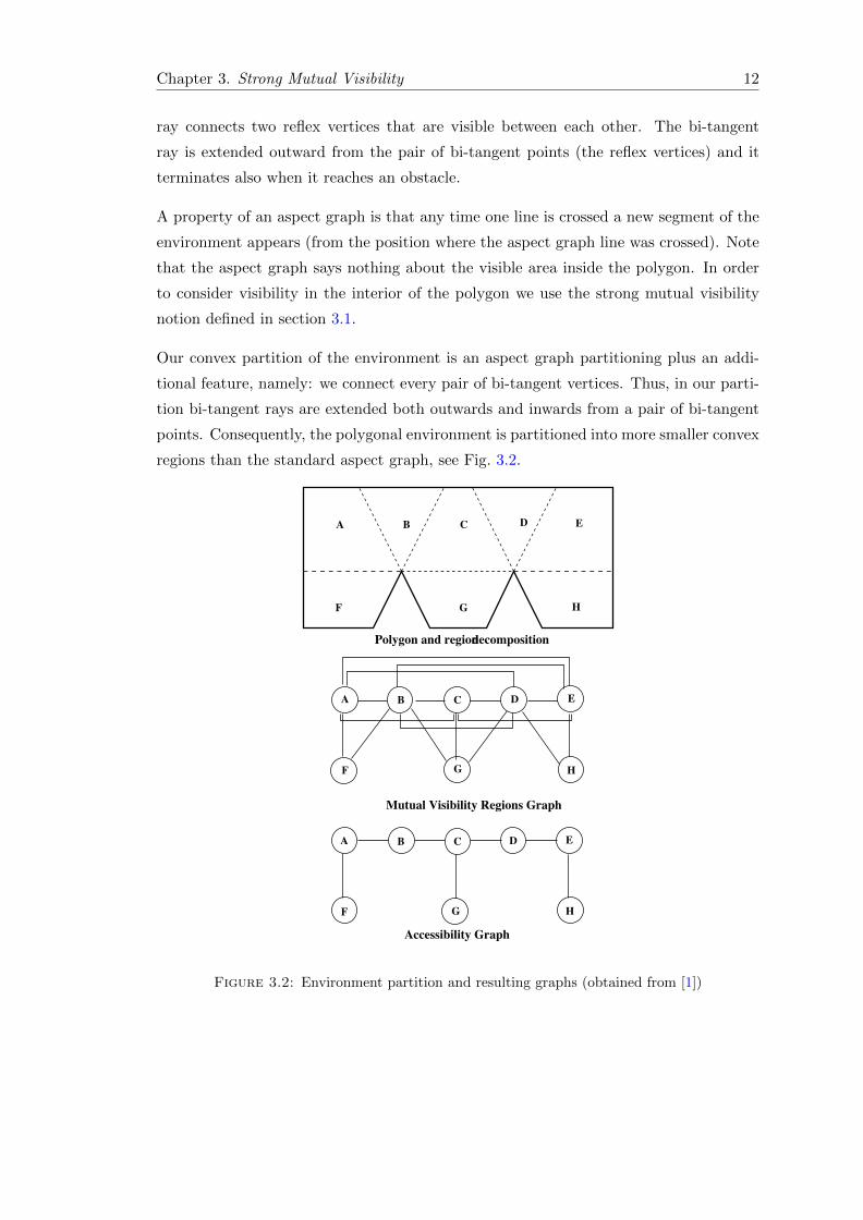
Our convex partition of the environment is an aspect graph partitioning plus an addi-
tional feature, namely: we connect every pair of bi-tangent vertices. Thus, in our parti-
tion bi-tangent rays are extended both outwards and inwards from a pair of bi-tangent
points. Consequently, the polygonal environment is partitioned into more smaller convex
regions than the standard aspect graph, see Fig. 3.2.
C D E
F G H
A B
A B DC E
F HG
Polygon and regiondecomposition
Accessibility Graph
Mutual Visibility Regions Graph
E
F H
A B C D
G
Figure 3.2: Environment partition and resulting graphs (obtained from [1])

Chapter 3. Strong Mutual Visibility 13
3.3 Finding strongly mutually visible regions
To define whether or not two regions are strongly mutually visible we use a convex hull
computation [70]. Formally we say that regions A and B are strongly mutually visible
if and only if int[convex-hull(A ∪ B)] ⊂ W , where W is the polygon representing the
workspace. In Fig. 3.2, regions A and E are strongly mutually visible; by contrast,
regions C and H are not.
3.4 Two graphs modeling the environment
The partition of the environment yields two graphs, one called Accessibility Graph (AG)
and the other Mutual Visibility Graph (MVG). In each graph, nodes represent regions.
In an AG, two nodes Ri and Rj are connected, written (Ri, Rj) ∈ AG, if their associated
regions share a region boundary bigger than one single point. Likewise, in an MVG, two
nodes Ri and Rj are connected, written (Ri, Rj) ∈ MVG, if their associated regions are
strongly mutually visible. Using the MVG and their current positions, each participant
is able to know both which regions are candidates to attempt to escape, called escapable
regions, and which regions the pursuer should move to if an escape is to be prevented,
called prevention-from-escape regions.
An MVG therefore provides information to find a sufficient condition to maintain evader
visibility while an AG provides possible region transitions that either participant can
carry out. Note that what counts as an escapable (respectively prevention-from-escape)
region depends on the current regions where both the evader and the pursuer are. More
precisely, let Ei (respectively Pj) denote that the evader (respectively the pursuer) is at
region Ri (respectively Rj). For each pair 〈Ei, Pj〉, denoting a problem configuration,
the set of escapable regions, written Re(i,j) ⊆ int(W ), is given by R : (Rj , R) /∈ MVG.
Moreover, for every escapable region R ∈ Re(i,j), there is a set of prevention-from-escape
regions, written Rp(i,j)(R) ⊆ int(W ), given by R′ : (R′, R) ∈ MVG.
Fig. 3.2(B) and (C) respectively show the MVG and the AG associated to the partition
of the environment shown in Fig. 3.2(A).
Chapter 3. Strong Mutual Visibility 14
3.5 Preventing From Escape Constrain
Given a problem configuration, 〈Ei, Pj〉, the primary constraint governing pursuit-evasion
is given as a relation on two times: the time taken for the evader to reach an es-
capable region, te(Re〈i,j〉), for some Re〈i,j〉 ∈ Re(i,j), and the time taken for the pur-
suer to reach one associated prevention-from-escape region, tpe(Rpe(Re〈i,j〉)), for some
Rpe(Re〈i,j〉) ∈ Rp(i,j)(Re〈i,j〉).
For the pursuer to prevent the evader from going to an escapable region, the constraint
te(Re〈i,j〉) ≥ tpe(Rpe(Re〈i,j〉))must be satisfied at all times, for all Re〈i,j〉 ∈ Re(i,j), and
for some Rpe(Re〈i,j〉) ∈ Rp(i,j)(Re〈i,j〉) for each Re〈i,j〉 ∈ Re
(i,j). Considering that both
pursuer and evader travel a given path, possibly at a different speed, this constraint can
be defined in terms of distances and relative velocities:
de(E(e), Re〈i,j〉) ≥ dpe(P (pe), Rpe(Re〈i,j〉))VeVp
(3.1)
where Ve and Vp are respectively the speed of the evader and the pursuer, and E(e) and
P (pe) are the positions of the evader and the pursuer. It is worth noticing that de and
dpe are, in general, geodesic distances [75].
This formulation holds for polygons with or without holes. However, in polygons with
holes a faster evader can always escape pursuer surveillance following a simple strat-
egy: turn around the nearest hole. Conversely, a faster pursuer, without surveillance
distance constraint, may apply another simple strategy: catch the evader (moving to a
configuration in contact with him) and then stick to him.
However, in polygons without holes, it is possible for a slower pursuer to keep visibility
of a faster evader. For instance, for an environment containing one single corner (we
refer to a reflex vertex), if the pursuer is at the corner, then he needs not to move at
all to avoid the evader from escaping. Even for more complex polygons, provided they
have no holes, a slower pursuer may always maintain visibility of a faster evader. So
a careful inspection on the map and the initial position of both participant is required
to determine the existence of a solution. Our approach is also able to find a winning
pursuer motion strategy if a solution exists.
Our pursuit-evasion problem can be abstracted to a graph: whether or not it is solvable
amounts to whether or not the graph enjoys some properties. However, the problem
still has a geometric aspect, namely: finding paths to move across regions. This problem
corresponds to assigning the appropriate weights to the graph edges.

Chapter 3. Strong Mutual Visibility 15
Clearly, if the pursuer is faster than the evader, then he will have a winning strategy in
a larger number of environments.
In [1], it is assumed an antagonistic evader who moves continuously but not unpre-
dictably due to he follows a fixed policy: travel the shortest path to escape pursuer
surveillance. Notice that it would be misleading to conclude that by making the evader
stick to an escaping policy our problem is no longer a game. To begin with, policies are
popular in games. For instance, in tic-tac-toe an unbeatable strategy starts by system-
atically choosing the center bean in the grid. What makes the problem presented in [1]
a non cooperative game is that the evader and pursuer have antagonistic goals [71]: the
evader aims to maximize gain by seeking for a time to escape, te, strictly smaller than
the time to prevent escaping, tpe; while the pursuer aims to minimize loss by keeping
tpe ≤ te.
We will introduce an approach that determines whether or not it is possible for a pursuer
to maintain strong mutual visibility of a moving evader, addressing the question: can the
evader escape? Further, whenever a solution exists, we will find a motion plan for the
pursuer that guarantees surveillance of the moving evader under the given assumptions.
In the next chapters of this thesis, we assume that the pursuer does not know the motion
policy of the evader, who moves continuously and antagonistically, and that the pursuer
is not able to predict the evader motion policy or to learn it. However, it is assumed
that the pursuer knows where the evader will be after a small progress of time, ∆t. So,
the pursuer is able to know the positioning of the evader, from t to t+ ∆t. Under such
setting, we deal with the problem of discovering pursuer motion strategies that are able
to maintain strong mutual visibility of the evader.

Chapter 4
The Effect of Incomplete
Information Over the Paths to
Escape
The authors of [1] have shown in that paper that traveling the shortest-path to reach an
escapable region is the best policy for the evader if the pursuer knows which escapable
region the evader is aiming to.
We now show that shortest path is not always the best escape policy in the more general
case, where the pursuer does not know which region, among a collection, the evader will
choose to go in an attempt to escape. In fact, we will show that there exist cases for
which the evasion is plausible only under the proviso that the evader does not adopt the
shortest path to escape policy.
The careful reader will have already noticed that our result takes the form:
∃x.(MayEscape(E, x) ∧ ¬Follows(E,ShortestPath)) (4.1)
where x ranges over configurations and E stands for the evader. Theorem (4.1) accounts
for a counterexample to the appealing conjecture:
∀x.(MayEscape(E, x)→ Follows(E,ShortestPath)) (4.2)
which happens not to be a theorem.1 Clearly, there are infinitely too many configurations
for which the shortest path policy enables the evader to escape. Producing any one such
1Indeed, we arrived at (4.1) in an attempt to prove (4.2).
16

Chapter 4. The Effect of Incomplete Information 17
an instance is trivial even for a primary school pupil. Even though all these success
cases, (4.2) is not a theorem.
Our non-trivial result, (4.1), holds regardless of whether the evader is slower or faster
than the pursuer. Let us consider first the case of a faster evader.
4.1 The Case of a Faster Evader
Proposition 4.1. There exist cases where a faster evader can escape only if it does not
travel the shortest distance from its initial position to an escapable region.
Proof. Fig. 4.1 depicts the scenario in which we elaborate our proof. There, E stands
for the evader, P for pursuer. Let A(p) denote that player A is at distinguished point
p ∈ <2.
R A
R Ad(2, )
R A
R A
!!>0
3
2
R B
R B’ A’R
d(3, )’
kd(k, )
Ve=Vp+
Figure 4.1: Evader faster than the pursuer
For the initial system configuration, (E(2), P (3)), there are two escapable regions,
RA and RB, each of which has two prevention from escape regions, RA, RA′ and
RB, RB′, respectively. Given that strong mutual visibility holds, then if the evader,
traveling the shortest path distance, goes to either RA or RB, the pursuer is able to
prevent escape correspondingly going to either the nearest point that belongs to RA′
or RB′ . That is because we constructed the map in such a way that d(E(2), RA) >
d(P (3), RA′)V eV p and d(E(2), RB) > d(P (3), RB′)V e
V p . Notice that the pursuer always
goes to the nearest prevention from escape region; this explains why going to RA or RB
is not considered as an option.

Chapter 4. The Effect of Incomplete Information 18
Now notice that if the evader first goes to point k, then he will simultaneously diminish
the distance to both escapable regions. We emphasize that moving this way the evader
is not travelling the shortest path to any of either escapable regions (indeed, along this
way it is not even moving toward an escapable region). But notice that the pursuer
cannot achieve a similar goal: move to a place where the distance to both prevention
from escape regions, RA′ and RB′ simultaneously diminishes. Once at k, the evader has
a wining move, given that he is faster than the pursuer. This is because d(E(k), RA) =
d(P (3), RA′) and d(E(k), RB) = d(P (3), RB′). It follows, that the evader can escape
only when it does not travel the shortest path to escape from its initial position.
The rationale behind this escape is that the pursuer does not know where the evader is
heading at in a long term and so he has to take into account all possible escape regions.
In the next section we consider the second case, where the evader is slower than the
pursuer.
4.2 The Case of a Slower Evader
Proposition 4.2. There exist scenarios for which a slower evader can escape only if it
does not travel the shortest distance from its initial position to an escapable region.
Proof. Refer to Fig. 4.2.
x
y
Figure 4.2: Evader slower than the pursuer

Chapter 4. The Effect of Incomplete Information 19
At first, the evader is at position E(2) and the pursuer at P (3), and thus the system
configuration is (E(2), P (3)). Let a and b respectively be the nearest point both to
escapable regions RA and RB, and on the other hand RA, RA′ and RB, RB′ are
the respective prevention from escape regions. Let r1 = d(k, a), r2 = d(2, a) and r3 =
d(3, RA′) and assume that r1 < r2 < r3. Without loss of generality, assume that both
players move at saturated speed and that Vp = r3r2Ve. Then, the time that the evader
needs to travel r2 equals the time the pursuer needs to travel r3, that is te = tpe when
the evader is at position E(2) and the pursuer at P (3).
For the next part of this proof, we will consider the next parameters for the proposed
example: r1 = 1, r2 = 2, r3 = 5√2
2 , h = 4, Ve = 1, d(2, 2′) = 1, d(3, 3′) = 5√2
4 and
m1 = 1, which is the slope of the straight line l1 which passes through the vertex a.
First, notice that, under these conditions (specially due to the chosen players’ velocities),
if the evader attempts to reach a traveling r2, the pursuer would be able to catch up
traveling r3. However, if the evader moves towards k (not travelling the shortest path
to any of either escapable regions), the pursuer would attempt to move to a place that
simultaneously reduces the distance that separates him from both RA′ and RB′ , that
is, also towards point k.2 But then the pursuer is bound to fail. This is because when
the evader reaches the position E(2′), the pursuer can be at must at position P (3′) and
for this system configuration, the time to escape (time for the evader to reach a) is
te ≈ 1.239 , while the time to prevent the escape (time for the pursuer to reach RA′) is
tpe ≈ 1.293, which clearly means that te < tpe, producing the imminent escape of the
evader. So finally we conclude that when the system initial configuration is (E(2), P (3)),
we have that te = tpe, but when the evader does not follow the shortest distance from
his initial position to an escapable region, he can take the system to the configuration
(E(2′), P (3′)), where te < tpe. The result follows.
A deeper analysis about the example shown in Fig. 4.2 can be performed, so is what
we will do next. The next analysis will be focused on the escape point a but a similar
analysis can be done respect to b due to the symmetry of the map and without forgetting
that the pursuer must deal with both escape points at once. Assuming the same initial
conditions depicted in proposition 4.2, notice that, as we did before, under these initial
conditions if the evader attempts to reach a traveling r2 (the shortest distance to reach
RA), the pursuer would be able to catch up, traveling r3 (the shortest distance to prevent
an evader’s escape through a). However, if the evader goes to k he would diminish
simultaneously his distance to a and b (again we emphasize that moving this way the
evader is not travelling the shortest path to any of either escapable region ), so the
2In what follows, we omit from our reasoning the prevention of a escape onto b, but recall that thepursuer must deal with both escape points at once.

Chapter 4. The Effect of Incomplete Information 20
pursuer would attempt to move to a place that also simultaneously reduces his distance
to both RA′ and RB′ (his closest prevention from escape regions), this would be to move
through the dotted line towards k.
We know that if the players follow this strategy at the beginning te = tpe due to the
selected velocities of the players but what we will do next is to analyse how the time to
escape te and the time to prevent the escape tpe will evolve as both players move over
the dotted line towards point k. Notice that we will only analyse the trajectories over
the dotted line because they are the ones that simultaneously diminish both the evader’s
distance to regions RA, RB and the pursuer’s distance to regions RA′ , RB′, without
establishing a preference over a specific region.
For the evader we will denote (xE(t), yE(t)), as his position as a function of time over
the dotted line starting from point 2 towards point k, e.g. E(2) = (xE(0), yE(0)). Based
on this we can also build an expression as a function of time for the distance to escape
from point (xE(t), yE(t)) through point a = (xa, ya) (the closest point of region RA from
the evader’s position). This expression is built as the distance from point (xE(t), yE(t))
to the point a as shown in equation (4.3). Then, making point 3 as the center of our
coordinate system (0, 0), taking into account that (xE(t), yE(t)) = (0, Vet+ d(3, 2)) and
that (xa, ya) = (−r1, h), we obtain equation (4.4). Finally based on equation (4.4) we
obtain the expression that shows how the time to escape through point a evolves as a
function of time; this final expression is shown in equation (4.5).
fde(t) =
√(xa − xE(t))2 + (ya − yE(t))2 (4.3)
fde(t) =
√r21 + (d(2, k)− Vet)2 (4.4)
fte(t) =fde(t)
Ve(4.5)
Similarly as we did before for the evader, for the pursuer we denote (xP (t), yP (t)), as his
position as a function of time over the dotted line starting from point 3 towards point
k, e.g. P (3) = (xP (0), yP (0)). What we will do next is to formulate an expression as a
function of time for the time to prevent the escape of the evader through point a. This
formulation will be based on the straight lines l1 and l3, both shown in Fig. 4.2. l1 is
the line that passes through point a with slope m1 which is defined by the map and
that contains the inflexion ray that prevents the evader’s escape through a. l3 will be a
perpendicular line to l1 that passes through (xP (t), yP (t)) which contains the shortest
path from the pursuer’s position to region RA′ . Both lines are described respectively by
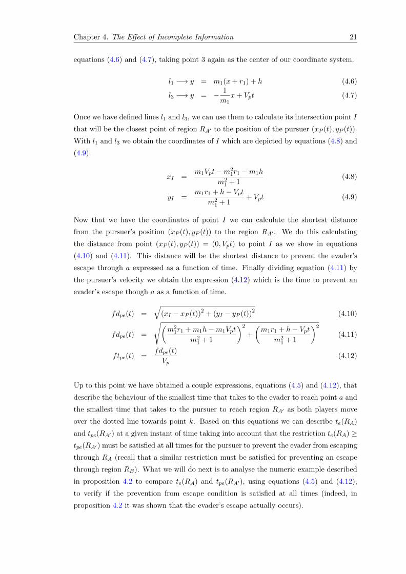
Chapter 4. The Effect of Incomplete Information 21
equations (4.6) and (4.7), taking point 3 again as the center of our coordinate system.
l1 −→ y = m1(x+ r1) + h (4.6)
l3 −→ y = − 1
m1x+ Vpt (4.7)
Once we have defined lines l1 and l3, we can use them to calculate its intersection point I
that will be the closest point of region RA′ to the position of the pursuer (xP (t), yP (t)).
With l1 and l3 we obtain the coordinates of I which are depicted by equations (4.8) and
(4.9).
xI =m1Vpt−m2
1r1 −m1h
m21 + 1
(4.8)
yI =m1r1 + h− Vpt
m21 + 1
+ Vpt (4.9)
Now that we have the coordinates of point I we can calculate the shortest distance
from the pursuer’s position (xP (t), yP (t)) to the region RA′ . We do this calculating
the distance from point (xP (t), yP (t)) = (0, Vpt) to point I as we show in equations
(4.10) and (4.11). This distance will be the shortest distance to prevent the evader’s
escape through a expressed as a function of time. Finally dividing equation (4.11) by
the pursuer’s velocity we obtain the expression (4.12) which is the time to prevent an
evader’s escape though a as a function of time.
fdpe(t) =
√(xI − xP (t))2 + (yI − yP (t))2 (4.10)
fdpe(t) =
√(m2
1r1 +m1h−m1Vpt
m21 + 1
)2
+
(m1r1 + h− Vpt
m21 + 1
)2
(4.11)
ftpe(t) =fdpe(t)
Vp(4.12)
Up to this point we have obtained a couple expressions, equations (4.5) and (4.12), that
describe the behaviour of the smallest time that takes to the evader to reach point a and
the smallest time that takes to the pursuer to reach region RA′ as both players move
over the dotted line towards point k. Based on this equations we can describe te(RA)
and tpe(RA′) at a given instant of time taking into account that the restriction te(RA) ≥tpe(RA′) must be satisfied at all times for the pursuer to prevent the evader from escaping
through RA (recall that a similar restriction must be satisfied for preventing an escape
through region RB). What we will do next is to analyse the numeric example described
in proposition 4.2 to compare te(RA) and tpe(RA′), using equations (4.5) and (4.12),
to verify if the prevention from escape condition is satisfied at all times (indeed, in
proposition 4.2 it was shown that the evader’s escape actually occurs).

Chapter 4. The Effect of Incomplete Information 22
As we did in proposition 4.2 we will use the next parameters values: r1 = 1, r2 = 2, h = 4,
m1 = 1 and Ve = 1. Once we have defined these parameters the whole system shown in
Fig. 4.2 is completely defined. In Fig. 4.3 a comparison plot is shown between te(RA)
and tpe(RA′) calculated respectively with functions fte(t) and ftpe(t). The horizontal
axis refers to the instants of time as both players move over the dotted line in Fig. 4.2
towards point k. This plot starts with a time value t = 0 that refers to the instant
of time when the evader is at E(2) and the pursuer at P (3), and the plot ends with a
time value t = tf that represents the instant of time when the evader arrives to E(k).
Analysing Fig. 4.3 we can see that at t = 0 we have te(RA) = tpe(RA′), this is due to
the way that we selected the velocity Vp of the pursuer. This also means that if at t = 0
the evader decides to follow the shortest path to region RA in an attempt to escape,
the pursuer will be in no trouble to prevent the escape because he can arrive to region
RA′ at the same time that the evader arrives to RA. Immediately after t = 0 something
interesting happens, namely, the curve referring to te(RA) finds itself bellow the curve
that refers to tpe(RA′) and this behaviour continues up to t ≈ 1.3, which means that if
in this interval of time the evader decides to move straight forward to RA we will have
that te(RA) < tep(RA′), producing an imminent escape of the evader. Also notice from
Fig. 4.3 that if the evader decides to keep moving over the dotted line towards point k
after t ≈ 1.3 the prevention from escape restriction is fulfilled again, te(RA) ≥ tpe(RA′),
so the pursuer again will be able to prevent the evader’s escape.
0.0 0.5 1.0 1.5t
1.0
1.5
2.0
2.5
ftpeHtL
fteHtL
ftpeHtL
fteHtL
Figure 4.3: Comparison between fte (t)↔ te (RA) and ftpe (t) ↔ tpe (RA′).
All the past analysis is truly important because it means that if from the starting
positions the evader decides to follow the shortest path to an escapable region he won’t
be able to escape but if he decides to follow other path which is not the shortest path to
escape, he can take the whole system into a configuration that will eventually produce
an inevitable escape of the evader. Table 4.1 shows some statistics concerning with the
proposed example.

Chapter 4. The Effect of Incomplete Information 23
Parameter V alue
r1 1r2 2h 4
m1 1Ve 1
r3 3.53553Vp 1.76777tf 1.73205
fte(0) 2ftpe(0) 2fte(0.5) 1.5868ftpe(0.5) 1.64645fte(1.0) 1.23931ftpe(1.0) 1.29289fte(tf ) 1ftpe(tf ) 0.77525yE(tf ) 1.73205yP (tf ) 3.06186
Table 4.1: Example parameters for the case of a slower evader.
Thus, together, propositions 4.1 and 4.2, show that (4.2) is indeed not a theorem: there
exists cases where an evader can escape only if it does not take the shortest path to
escape, one of the key contributions of this thesis. The main idea behind this result
is that there are cases where the evader has the ability to maintain the uncertainty of
which escapable region he will finally choose while he follows a path (which is not the
shortest path to neither escapable region) that simultaneously reduces his distance to
several escapable regions which eventually will lead to a smaller time to escape than the
time to prevent the escape, despite the fact that the pursuer may be also simultaneously
reducing his distance to the respective prevent from escape regions.

Chapter 5
Keeping or Escaping Pursuer
surveillance
Any solution to the problem of determining whether or not the pursuer is able to main-
tain evader surveillance on a given environment depends on two main factors: (i) the
initial position of both participants; and (ii) the long-term combinatoric paths that the
evader can travel over the environment in an attempt to escape. We will study both
factors below. We formulate our problem as a game and so, for every match, we will
determine which among the pursuer or the evader has a winning strategy.
5.1 Players Strategies and Paths
We have found that under the definition of strong mutual visibility, the possible paths
that the evader can travel to escape can be classified in two types: 1) paths where the
evader escapes when he does not touch a reflex vertex 1 in the environment; 2) paths
where the evader escapes but the opposite condition holds, namely, the escape happens
touching a reflex vertex. Notice that we can generate a more general type of paths which
is constructed as combination of paths of type 1) and 2).
The first type of paths do not lie on the reduced visibility graph (a brief description of
the reduced visibility graph is given in appendix A). Fig. 5.1 A) shows a path of type
1). As before, the environment is the polygon shown with back solid lines, the region
partition is shown with dashed lines and the regions are labeled with numbers. The
evader is at region 1 and the pursuer at region 21. If the evader goes directly to region
1Recall that, a reflex vertex is one of an internal angle greater than π.
24

Chapter 5. Keeping or Escaping Pursuer surveillance 25
2, then the pursuer must go to region 12 (the closest prevention from escape region from
the current pursuer’s position).
Figure 5.1: Paths types
Arrows represent paths. P stands for the pursuer and E for the evader. These paths
cannot be characterized based only on the reflex vertices positions. But notice that
Equation (3.1) can be used to determine whether or not at a given time the evader can
escape. At all instants of time, based on the position of the players, together with the
MVG and the AG, it is possible to decide whether or not the evader has a winning move.
For the evader to travel the second type of paths, he may move along the reduced
visibility graph [70]. The motivation for the evader to do so is that firstly the reflex
vertices, which belong to the reduced visibility graph, by definition break the convexity
of a polygon, and secondly, in a 2D polygonal environment the shortest path connecting
two positions that do not see each other is related to the reduced visibility graph [72],
hence, this graph will be also related to the smallest time to escape when having such
configurations.
Fig. 5.1 B) shows a path of type 2). Initially the evader is at region 20 and the pursuer
at region 21. For this scenario the closest escapable region for the evader is the one
labeled with 14, and the shortest path for reaching it is moving straight forward to a

Chapter 5. Keeping or Escaping Pursuer surveillance 26
reflex vertex and moving around it. In this case to prevent the escape the pursuer must
arrive to region 17 (again the closest one to prevent the escape) at least at the same
time that the evader reaches region 14.
As we stated in the problem definition in section 1.1 we address the problem of disco-
vering pursuer motion strategies that are able to maintain strong mutual visibility of the
evader considering that the global motion policy of it is unknown, but for this thesis we
will only focus on paths of type 2), that is, we will restrict the evader to escape only by
touching reflex vertices. Taking into account the paths of type 1) as possible escapable
paths for the evader, will be left as future work.
5.2 Initial Conditions
Finding a winner to an instance of our game depends clearly on the initial position of both
players, as well as their corresponding maximum speed. There might be configurations
that either player would find unpleasant. Consider, for instance, the case where, even
though strong-mutual visibility holds, the players are so apart one another that, to
escape, the evader may just need to go to the adjacent region. To see a concrete example
of this case, refer to Fig. 4.2. If the pursuer and the evader respectively are at point a
and b and if neither player is faster than the other, then the evader will be in no troubles
at all to escape.
Given an instance of the problem, to determine whether or not there is still a game,
we proceed as follows. First, use the MVG and the AG, together with equation (3.1),
to find out whether there is a escapable region that the evader can reach in a time
strictly smaller than that needed by the pursuer to reach a corresponding prevent-from-
escape region. If there does not exist any such escapable region, the game continues,
this means that we still need to verify if the long term paths that the evader can follow
do not produce an escape. If from the beginning such an escapable region exists there is
a winning path for the evader that can be verified just by taking into account the initial
positions of the players.
Our method performs similarly to that of [73], even though the latter method considers
classical visibility2. This is because, in this case, building a compact set is analogous
to identifying whether the evader is able to reach a escape region before the pursuer
prevents the escape.
2In classical visibility, two points see one another if the line segment between them does not cross anobstacle.

Chapter 5. Keeping or Escaping Pursuer surveillance 27
5.3 Combinatoric Paths
Determining which player has a winning strategy also depends on the long term paths
that the evader can follow. This situation is depicted in Fig. 5.2. In this example
the path of the evader is coloured in red (wide-dashed lines) and the ones followed by
the pursuer are coloured in blue (wide-solid lines). We assume that Vp = Ve. It can
be appreciated that the evader follows a path of type 2) as we defined in section 5.1,
starting at position E(1) and ending at reflex vertex Rv2. For this given path for the
evader and taking into account that the pursuer starts at position P (2) two possible
escape situations may occur, the first when the evader arrives at reflex vertex Rv1 and
the second one when he arrives to reflex vertex Rv2. For paths of type 2) when the
evader arrives to a reflex vertex, it is sufficient for the pursuer to arrive at the same time
to some point of his closest inflection ray related to such vertex, to prevent the escape.
Following this idea in our example, when the evader arrives to E(Rv1) it is sufficient for
the pursuer to arrive at the same time to any point belonging to the inflexion ray Ir1 as
it is shown in Fig. 5.2 A), where the pursuer arrives to P (3). The problem here is that
if the pursuer arrives to a point that belongs to Ir1 which is too far away from Ir2, he
will be able to prevent a first attempt of the evader to escape through Rv1 but when the
evader arrives to Rv2 the pursuer won’t make it on time into the second inflexion ray
Ir2, producing the escape of the evader. Such scenario is shown in Fig. 5.2 A) where
d(1, Rv1) > d(2, 3) but d(Rv1, Rv2) < d(3, 4), producing the escape of the evader in his
second attempt to escape touching Rv2.
1 1
2 23 3
3'
44
EP
A) B)
Figure 5.2: Long Term Paths
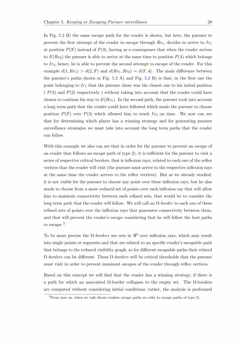
Chapter 5. Keeping or Escaping Pursuer surveillance 28
In Fig. 5.2 B) the same escape path for the evader is shown, but here, the pursuer to
prevent the first attempt of the evader to escape through Rv1, decides to arrive to Ir1
at position P (3′) instead of P (3), having as a consequence that when the evader arrives
to E(Rv2) the pursuer is able to arrive at the same time to position P (4) which belongs
to Ir2, hence, he is able to prevent the second attempt to escape of the evader. For this
example d(1, Rv1) > d(2, 3′) and d(Rv1, Rv2) = d(3′, 4). The main difference between
the pursuer’s paths shown in Fig. 5.2 A) and Fig. 5.2 B) is that, in the first one the
point belonging to Ir1 that the pursuer chose was the closest one to his initial position
( P (3) and P (2) respectively ) without taking into account that the evader could have
chosen to continue his way to E(Rv1). In the second path, the pursuer took into account
a long term path that the evader could have followed which made the pursuer to choose
position P (3′) over P (3) which allowed him to reach Ir2 on time. We now can see
that for determining which player has a winning strategy and for generating pursuer
surveillance strategies we must take into account the long term paths that the evader
can follow.
With this example we also can see that in order for the pursuer to prevent an escape of
an evader that follows an escape path of type 2), it is sufficient for the pursuer to visit a
series of respective critical borders, that is inflexion rays, related to each one of the reflex
vertices that the evader will visit (the pursuer must arrive to the respective inflexion rays
at the same time the evader arrives to the reflex vertices). But as we already studied,
it is not viable for the pursuer to choose any point over these inflexion rays, but he also
needs to choose from a more reduced set of points over each inflexion ray that will allow
him to maintain connectivity between such refined sets, that would be to consider the
long term path that the evader will follow. We will call an Ω-border to each one of these
refined sets of points over the inflexion rays that guarantee connectivity between them,
and that will prevent the evader’s escape considering that he will follow the best paths
to escape 3.
To be more precise the Ω-borders are sets in <2 over inflexion rays, which may result
into single points or segments and that are related to an specific evader’s escapable path
that belongs to the reduced visibility graph, so for different escapable paths their related
Ω-borders can be different. These Ω-borders will be critical thresholds that the pursuer
must visit in order to prevent imminent escapes of the evader through reflex vertices.
Based on this concept we will find that the evader has a winning strategy, if there is
a path for which an associated Ω-border collapses to the empty set. The Ω-borders
are computed without considering initial conditions; rather, the analysis is performed
3From now on, when we talk about evaders escape paths we refer to escape paths of type 2).
Chapter 5. Keeping or Escaping Pursuer surveillance 29
in a steady-state condition, where only the path determines the size and shape of each
Ω-border.
To compute every Ω-border, we make the evader to travel every single shortest-time
path starting on a reflex vertex and visiting any other reflex vertex. We make the
evader travel all this paths because we don’t know where the evader is heading in a
long term; the pursuer just knows where the evader will be after a small progress of
time, ∆t, as we stated in the problem definition in section 1.1. Hence, we try to capture
all possible evader’s escapable paths to deal with the uncertainty of which trajectory
will the evader finally choose in order to generate a pursuer’s strategy that englobes all
such possibilities. As it can be seen, we based the computation of the Ω-borders on
the shortest paths between reflex vertices, without considering the current positioning
of the players but rather considering the structure of the map, in order to deal with the
combinatorial part of the problem. Further in this section we will introduce the method
that we call the S set, which is computed based on the current position of the players
and which will allow us to deal with evader’s paths that are not necessarily the shortest
ones.
The previously mentioned shortest paths are all in the reduced visibility graph [70]. We
are interested only in paths of the reduced visibility graph mainly due to two main
reasons. First, because any time the evader reaches a reflex vertex a new possibility
for an escape comes up. This is in turn because every reflex vertex, by definition,
breaks convexity of the environment. Also recall that we mentioned in section 5.1 that
we would only consider evader’s escapes touching reflex vertices. Second, the reduced
visibility graph will contain all the shortest paths between reflex vertices that belong to
an escapable path.
The rationale behind the algorithm that we will present is to find out whether the pursuer
can keep surveillance (respectively, the evader can escape) at a long-term, assuming valid
initial conditions and that the evader travels the reduced visibility graph, choosing a visit
ordering which aims to make the time to escape smaller than the time to prevent escape.
Notice that this involves dealing with an intractable problem [1].
Below, we present our algorithm which plans pursuer motions so as to keep track of
an evader who does not necessarily travel the shortest paths to an escapable region.
This algorithm consists of two methods. The first method uses the network of shortest
distances traveled by the evader between escapable regions in order to define valid points
for the pursuer to prevent escapes. These points, which depend on the velocity of both
players, form the Ω-borders. The second method uses Ω-borders to compute a region in
the plane where the pursuer must be in order to prevent the evader from escaping. We
call this region S, for solution set. S ∈ <2 is a set of points, which guarantee that at a

Chapter 5. Keeping or Escaping Pursuer surveillance 30
given instant of time, the evader cannot reach a reflex vertex in a time strictly smaller
than the time that the pursuer needs to reach its associated Ω-border.
It is important to underline that while the Ω-borders are computed assuming that the
evader travels moving in the network of shortest paths between reflex vertices, the Ω-
borders are used to prevent the escaping of the evader even if he does not move traveling
those shortest paths thanks to the usage of the S set (in section 5.3.2 we will go deeply
into the computation of the S set).
5.3.1 Ω borders
Before presenting the algorithm to compute the Ω-borders, we need to define some
preliminary concepts.
Let vl be a reflex vertex in the polygonal workspace W . Inciding in vl, there are two
segments of W . Conversely, emerging from vl there are two inflection rays of the aspect
graph [74]. For each vertex vl, we order its associated inflection rays using a counter-
clockwise ordering. Thus, the first inflection ray of vl on this ordering is called rl,1 and
the second one rl,2. Fig. 5.3 shows an example of such ordering, presenting the inflexion
rays as dashed lines.
Figure 5.3: Inflexion rays ordering
Each inflection ray is a potential Ω-border, which is to be refined by our algorithm
below. Ω-border refinement depends on the paths that the evader travels over the
reduced visibility graph [70] (RVG). The evader might turn around any vertex either
clockwise or counter-clockwise. If the evader turns around counter-clockwise a vertex
vl, then it crosses the rl,1 inflection ray first; otherwise, it crosses rl,2 first.
Let V be the set of all reflex vertices in W . Then, we have to analyse all viable per-
mutational escapable paths (that is paths that conserves the connectivity of the RVG,
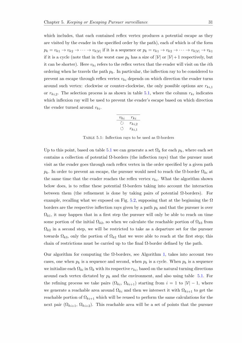
Chapter 5. Keeping or Escaping Pursuer surveillance 31
which includes, that each contained reflex vertex produces a potential escape as they
are visited by the evader in the specified order by the path), each of which is of the form
pk = vk1 → vk2 → · · · → vk |V| if it is a sequence or pk = vk1 → vk2 → · · · → vk |V| → vk1
if it is a cycle (note that in the worst case pk has a size of |V| or |V|+ 1 respectively, but
it can be shorter). Here vki refers to the reflex vertex that the evader will visit on the ith
ordering when he travels the path pk. In particular, the inflection ray to be considered to
prevent an escape through reflex vertex vki depends on which direction the evader turns
around such vertex: clockwise or counter-clockwise, the only possible options are rki,1
or rki,2. The selection process is as shown in table 5.1, where the column rki indicates
which inflexion ray will be used to prevent the evader’s escape based on which direction
the evader turned around vki.
vki rki rki,2 rki,1
Table 5.1: Inflection rays to be used as Ω-borders
Up to this point, based on table 5.1 we can generate a set Ωk for each pk, where each set
contains a collection of potential Ω-borders (the inflection rays) that the pursuer must
visit as the evader goes through each reflex vertex in the order specified by a given path
pk. In order to prevent an escape, the pursuer would need to reach the Ω-border Ωki at
the same time that the evader reaches the reflex vertex vki. What the algorithm shown
below does, is to refine these potential Ω-borders taking into account the interaction
between them (the refinement is done by taking pairs of potential Ω-borders). For
example, recalling what we exposed on Fig. 5.2, supposing that at the beginning the Ω
borders are the respective inflection rays given by a path pk and that the pursuer is over
Ωk1, it may happen that in a first step the pursuer will only be able to reach on time
some portion of the initial Ωk2, so when we calculate the reachable portion of Ωk3 from
Ωk2 in a second step, we will be restricted to take as a departure set for the pursuer
towards Ωk3, only the portion of Ωk2 that we were able to reach at the first step; this
chain of restrictions must be carried up to the final Ω-border defined by the path.
Our algorithm for computing the Ω-borders, see Algorithm 1, takes into account two
cases, one when pk is a sequence and second, when pk is a cycle. When pk is a sequence
we initialize each Ωki in Ωk with its respective rki, based on the natural turning directions
around each vertex dictated by pk and the environment, and also using table 5.1. For
the refining process we take pairs (Ωki, Ωki+1) starting from i = 1 to |V| − 1, where
we generate a reachable area around Ωki and then we intersect it with Ωki+1 to get the
reachable portion of Ωki+1 which will be reused to perform the same calculations for the
next pair (Ωki+1, Ωki+2). This reachable area will be a set of points that the pursuer

Chapter 5. Keeping or Escaping Pursuer surveillance 32
can reach from some point belonging to Ωki, in a time smaller or equal to the time that
it takes to the evader to travel the shortest distance between vki and vki+1 (Algorithm 3
gives more details about this reachable area). After doing the same calculation through
all pairs, we obtain a refined Ωk |V| that is reachable from Ωk1. The next step is to go
backwards through pairs (Ωki, Ωki−1) with i = |V| to 2, to recover the valid portions
of each Ωki that gave us the reachable portion of Ωk |V| from Ωk1. Similarly as we did
before, a reachable area around Ωki is generated and then it is intersected with Ωki−1
to get the correct portion of Ωki−1. We iteratively do the same procedure for all pairs.
At the end we obtain a valid Ωk1 that is a subset of rk1 which allow us to reach a valid
subset of rk |V| that is Ωk |V|.
One important thing to notice is that if at least one of the resulting Ω-borders related
to a given evader’s path happens to be a segment, then the resulting Ω-borders will
capture a family of pursuer’s paths that will prevent the evader from escaping through
the related escapable path (recall that each escapable path has its own set of Ω-borders).
We obtain a family of paths because the pursuer will have several points to choose from,
over the Ω-borders that resulted into segments. The only case when the Ω-borders
contain a unique pursuer’s path for their related evader’s escapable path, is when all the
Ω-borders resulted into single points.
When pk is a cycle the procedure is basically the same as the one for sequences. The
main difference is that the last Ω-border Ωk |V|+1 in Ωk refers to the same inflection
ray as Ωk1. We perform the same refining procedure described above to get a valid
Ωk1 to go to a valid Ωk |V|+1, but recalling that both Ωk1 and Ωk |V|+1 are subsets of
rk1 we have to do some extra analysis here. After refining the potential Ω-borders and
supposing that the evader would take this path, three things can occur. First, if Ωk |V|+1
is an empty set, this means that the pursuer can’t maintain visibility of the evader (the
evader wins the game). Second, if Ωk |V|+1 ⊆ Ωk1, this means that the pursuer would
be able to maintain visibility of the evader and he would be able to keep maintaining
it if the evader decides to take this path again and again. Third, if Ωk1 ⊆ Ωk |V|+1,
this means that the pursuer could maintain visibility of the evader but once they have
completed the first cycle, the pursuer could have ended in a non valid starting position
for a second cycle, in which case, we repeat the refinement procedure again until we find
ourselves in the first or second case described above (consult Algorithm 1 for more details
about such refinement procedure). Notice that since the length of the winning pursuer
paths are lower bounded by tours over the reduced visibility graph (the shortest evader’s
path), those tours provide a convergence condition for the algorithm for computing the
Ω-borders.

Chapter 5. Keeping or Escaping Pursuer surveillance 33
Algorithm 1 Computing Ω borders
Input: Work space, W , environment partition.Output: Ω borders.for every permutational path of the form
pk = vk1 → vk2 → · · · → vk |V| → vk1
orpk = vk1 → vk2 → · · · → vk |V|
do1. Considering the pair vki → vki+1, look up at Table 5.1 to determine the inflectionrays: rki and rki+1;2. Initialization. Ωk = Ωki : i ∈ N, 1 ≤ i ≤ n, where n = |V| for a sequence orn = |V|+ 1 for a cycle;for i = 1 to |V| do
A. Ωki ← rki;end forif pk is a cycle then
B. Ωk |V|+1 ← Ωk1;end if
C. bd← true;3. Ωk calculation;if pk is a cycle then
repeatA. Ωk |V|+1 ← Ωk1;B. Ωk ← ΩBdrsInteraction(Ωk, pk, |V|+ 1, bd);C. bd← false;
until Ωk |V|+1 ⊆ Ωk1 ∨ Ωk |V|+1 = φelse if pk is a sequence then
A. Ωk ← ΩBdrsInteraction(Ωk, pk, |V|, bd);end if4. Store(Ωk, pk);
end for
Algorithm 2 ΩBdrsInteraction(Ωk, pk, n, bd)
Input: Set Ωk composed by unrefined Ω borders related to pk, path pk, n length ofpk, bd flag that indicates that the calculation must be done in both directions;Output: Set Ωk with refined Ω borders due to the interaction between them.if bd == true then
for i = 1 to n− 1 do1. Ωki+1 ← Refine(Ωki,Ωki+1, vki, vki+1);
end forend iffor i = n to 2 do
2. Ωki−1 ← Refine(Ωki,Ωki−1, vki, vki−1);end forReturn Ωk;

Chapter 5. Keeping or Escaping Pursuer surveillance 34
Algorithm 3 Refine Ω borders, Refine(Ωka,Ωkb, vka, vkb)
Input: Ω border Ωka, Ω border Ωkb, reflex vertex vka and reflex vertex vkb.Output: refined Ω border.1. A = x ∈ R2 : d(p, x) ≤ d(vka, vkb)
Vp
Ve, p ∈ R2, p ∈ Ωka;
Return A ∩ Ωkb;
1
2
3
4 5
6
7
8 9 11
12
101
2
3
4 5
6
7
8 9 11
12
10
a ab b
c c d
A) B)
Figure 5.4: Ω borders
Consider Fig. 5.4. In both parts, the environment is the polygon shown with black solid
lines, the region partition is shown with dashed lines and the regions are labeled with
numbers. The polygon has 4 reflex vertices. The Ω-borders, computed setting V e = V p,
are shown in green color (wide dark-grey points and lines). In Fig. 5.4 A) the Ω-borders
were computed for an evader’s path that touches the vertices a → b → c; here, the
resulting Ω-borders are two points and one line segment. In Fig. 5.4 B) the Ω-borders
were computed for an evader’s escapable path that goes through all the reflex vertices
a → b → c → d; now the resulting Ω-borders are simply points. Notice that when the
vertex d is considered, the Ω-borders are reduced to the vertices themselves. This is
because the border of the partition regions and the vertices are equally separated one
another. Notice that in this environment, if we set Ve > Vp, then the Ω-borders would
be empty sets. Thus, in this environment, a faster evader will always win.
Fig. 5.5 shows how the Ω-borders in Fig. 5.4 A) where calculated using Algorithm 1.
For this map there are several potential escapable paths that can be built using the four
reflex vertices. In this example the evader’s escapable path that was considered is the
one that we call p1, which follows the next reflex vertices in the next order: a→ b→ c. It
is assumed that Vp = Ve. As we already mentioned the first thing to do is to identify the
inflexion rays that will prevent the evader’s escape through each one of the mentioned
reflex vertices. These inflexion rays are used to initialize the tree respective Ω-borders
that will be related to path p1. In Fig. 5.5 A) such inflexion rays were coloured in cyan
(wide light-grey lines). We will denote Ir1a as the selected inflexion ray for reflex vertex
a, Ir1b as the one selected for vertex b and Ir1c as the one selected for vertex c. In

Chapter 5. Keeping or Escaping Pursuer surveillance 35
A) B)
D)C)
F)E)
Figure 5.5: Ω borders calculation
each figure the refined Ω-borders are shown in green (wide dark-grey points and lines)
as they are calculated (here the Ω-borders will be refinements of the respective cyan—
light-grey— inflexion rays). For path p1, we will denote Ω-b1a as the Ω-border related
to reflex vertex a, Ω-b1b as the Ω-border related to b and Ω-b1c as the one related to c.
From Fig. 5.5 B) to Fig. 5.5 C), the refinement procedure to calculate the portion of
Ω-b1c that is reachable from Ω-b1a is shown. Then, from Fig. 5.5 D) to Fig. 5.5 E) it is
shown the backwards procedure for calculating the valid portion of each Ω1i that gave
us the reachable portion of Ω-b1c. The reachable areas used in each iteration are shown
in red (grey) color. Finally Fig. 5.5 F) shows the resulting Ω-borders for the evader’s
escapable path p1 = a → b → c. At the end we obtain a valid Ω-b1a that is a subset

Chapter 5. Keeping or Escaping Pursuer surveillance 36
of Ir1a which allow us to reach a valid subset of Ir1c that is Ω-b1c. In table 5.2 the
Ω-borders used to generate the reachable areas are shown, also with the Ω-borders that
are intersected with the respective areas and the respective distance taken into account
to generate each area (recall that Vp = Ve).
Forward Procedure
Figure Pivot Ωki Intersected Ωki+1 d(vki, vki+1)Vp
Ve
Fig. 5.5 B) Ω-b1a Ω-b1b d(a, b)Fig. 5.5 C) Ω-b1b Ω-b1c d(b, c)
Backward Procedure
Figure Pivot Ωki Intersected Ωki−1 d(vki, vki−1)Vp
Ve
Fig. 5.5 D) Ω-b1c Ω-b1b d(c, b)Fig. 5.5 E) Ω-b1b Ω-b1a d(b, a)
Table 5.2: Statistics for Ω-borders calculation example.
In general, computing Ω-borders requires dealing with a computationally intractable
problem [1]. However, we can find an approximate solution, for example, by computing
Ω-borders for a subset of reflex vertices. This would be useful if we clustered the vertices,
hence dividing the tour and then compute Ω-borders for each part of this tour. This
is equivalent to do local planning; the planning horizon would be determined by the
number of vertices to consider. This strategy will not guarantee surveillance at all times
but it is useful to make short term planning that prevent the evader from escaping.
Of course, for small polygons, e.g. with around 15 reflex vertices or so, it is actually
possible, using a regular PC, to compute the Ω-borders considering all reflex vertices.
5.3.2 Regions of Local Solution
S is the set of points where the pursuer must be to prevent the evader from going behind
a reflex vertex, vl, and hence escape. Let V be a subset of all reflex vertices that fulfill
the properties described in Proposition 5.1. Then, considering that the evader and the
pursuer respectively are at region Ri and Rj , S is defined by equation (5.1).
Proposition 5.1. V is a subset of all the reflex vertices which lie over a frontier between
a region that is strongly mutually visible and one that is not strongly mutually visible,
both with respect to Rj (region where the pursuer is located).
Proof. To begin with, lets call a critical frontier, a frontier between a region that is
strongly mutually visible and one that is not strongly mutually visible, both with respect
to Rj . First of all, all the vertices which are within a region mutually visible with Rj ,
that do not lie over a critical frontier, are not candidates to be taken as part of V because

Chapter 5. Keeping or Escaping Pursuer surveillance 37
they do not produce an escape to the evader. Furthermore, assuming that the evader
is within a region which is under surveillance (that is, the evader is in a region that
is mutually visible with Rj), for producing an escape the evader will need to move to
another region not mutually visible with Rj , and taking into account that the escapes
must take place going through a reflex vertex, this transition between regions must be
through a reflex vertex over the critical frontier of such regions. In other words, the only
way for the evader for leaving a region mutually visible with Rj and produce an escape
is through a reflex vertex lying over a critical frontier. So assuming that the evader is
under surveillance and that he wants to reach a reflex vertex which is within a region
that is not mutually visible with Rj but not over a critical frontier, then the evader will
necessarily pass through a reflex vertex lying over a critical frontier in order to reach
it. Based on this fact, we can ensure that all the possible escapes through the vertices
behind a reflex vertex over a critical frontier, will be considered on the construction of
the Ω-borders related to paths that start with such reflex vertex, hence, the only thing
left to do is to make sure that the pursuer reaches the correct Ω-border before the evader
reaches the reflex vertex over the critical frontier. This is done by placing the pursuer
inside the S set.
S = p ∈ R : (R,Ri) ∈MVG)∧
vl∈Vd(p,Ω(vl)) ≤ d(P (e), vl)
VpVe
) (5.1)
In equation (5.1), taking into account the current evader’s position, Ω(vl) denotes the
intersection of every Ωk1 that is related to a potential escapable path pk whose vk1 = vl,
and whose natural turning direction around vk1 is the same turning direction with
which the evader will attack vl. d(p,Ω(vl)) is the geodesic distance between the point
p and Ω(vl), d(P (e), vl) denotes also a geodesic distance, this time between the evader
position P (e) and vertex vl, and V the subset of all the reflex vertices, as described
in proposition 5.1 (that is, we consider only the reflex vertices that lie over a frontier
between a region that is strongly mutually visible and one that is not strongly mutually
visible, both with respect to Rj).
In Fig. 5.6 a sample S set is shown. The evader’s position is shown as a red (grey)
square and the pursuer’s one with a blue (small-grey) circle. In this case the set V just
contains the reflex vertex a because it is the only one that lies over a critical frontier,
that is the frontier between region 2 and region 3. For purposes of this example, lets
suppose that there is just one path whose vk1 = vl, and whose natural turning direction
around vk1 is the same turning direction with which the evader will attack vl (in Fig. 5.6
it is shown as an arrow around a), being that path the one that goes through vertices

Chapter 5. Keeping or Escaping Pursuer surveillance 38
EP
a b
c d
Figure 5.6: S set example
a → b → c → d. For this path its related Ω-borders are the four green (dark grey)
points shown in Fig. 5.6. Talking about Ω(vl), because it considers only one potential
escapable path, it returns the Ω-border respective to reflex vertex a. The resulting S
set is shown in Fig. 5.6 in yellow (light grey).
The region S is used to define a new valid pursuer position regardless the trajectory of
the evader. If the pursuer is inside the S set, it is guaranteed that at that given instant
of time, the evader cannot reach a reflex vertex in a time strictly smaller than the time
that the pursuer needs to reach its associated Ω-border. Thus, we have a method to
compute the pursuer motion, which is independent of the evader policy and path.

Chapter 6
Simulation Results
All our simulation experiments were run on a dual core processor PC, equipped with 1
GB of RAM, running Linux. Basically we present two types of results, the ones related
to evader’s escapable paths which are sequences and the ones related to escapable paths
that are cycles, as they were classified on section 5.3.1.
6.1 Paths of sequences’ type
Fig. 6.1 shows our simulation results corresponding to a first test environment. In these
figures, obstacles are shown in grey and the free space in white, regions are delimited
with line segments. The evader position is the red (grey) square and the pursuer is the
blue (small-grey) circle. The Ω borders are shown in green (dark-grey points and lines)
and the S set regions in yellow (light grey). In the simulation the velocity of the evader
was set equal to the velocity of the pursuer, V e = V p.
For obtaining these simulation results, first of all, the decomposition of the environment
into convex regions, the accessibility graph (AG) and the mutual visibility graph (MVG)
are computed and stored. Then the Ω borders for all possible escapable paths are also
computed and stored as well. For the environments presented in this section, the whole
set of possible escapable paths can be represented as sequences. It is important to take
into account that the possible escapable paths are obtained from the reduced visibility
graph (RVG); to retrieve the paths, what we do, is to consider each one of the nodes in
the RVG as a starting reflex vertex, then we consider all the possible paths from each
one of those starting reflex vertices to each one of the vertices contained in the RVG,
taking into account the connectivity of the graph and just considering paths that do not
contain repeated vertices. There is also a special type of paths that must be considered,
39

Chapter 6. Simulation Results 40
A) B)
C) D)
F)E)
Figure 6.1: Simulation Results – first simulation with paths of sequences’ type

Chapter 6. Simulation Results 41
which are paths composed of a single reflex vertex, in which case, both possible evader’s
turning directions around the reflex vertex must be taken into account, resulting into
two paths for each reflex vertex in the RVG and whose related Ω borders will result into
the whole corresponding inflexion rays (this is done by just consulting table 5.1). The
final stage is the computation of the S set, which will work as sort kind junction between
the Ω borders related to the potential escapable paths based on the current positions of
the players. The S sets are calculated in a on-line fashion as the players continuously
move around the environment.
For calculating the S sets we proceed in the next way: lets assume that at the time
index t, the evader and the pursuer are at the respective positions E(t) and P (t). As we
mentioned in section 1.1 the pursuer is able to know where the evader will be after a small
progress of time, ∆t, so the pursuer knows the evader’s position E(t + 1), considering
that the difference between the time stamp indexed by t and the one indexed as t+1 has
a difference of ∆t. Furthermore, to calculate the next position of the pursuer P (t+ 1),
what we do is to calculate the S set using equation (5.1) considering the positions of the
players E(t+ 1) and P (t). Finally we select from this S set, any point that is reachable
from the pursuer’s position P (t) within a time interval ∆t, and we make such point the
new pursuer’s position P (t+ 1).
In Fig. 6.1, snapshots are presented as the evader follows a path which does not belong
to the shortest paths to escape. For example, in Fig. 6.1 B), Fig. 6.1 C) and Fig. 6.1 D),
the evader moves downwards, then upwards and then downwards again, which is clearly
not a shortest path to produce an escape.
We also can see that in each one of the snapshots the S set is shown in conjunction with
its respective Ω borders that were used to calculate it; the used Ω borders may differ
between S sets. For instance, the Ω borders used to calculate the S set in Fig. 6.1 A)
are different from the ones used to calculate the S set in Fig. 6.1 B); in the fist case they
are points while in the second case they are points and a line segment. The Ω borders
differ because in both figures the players are in a different region, hence, the potential
escapable paths for the evader are also different, and because the Ω borders are related
to an specific escapable path, we had as a result that for the calculation of each S set we
used different Ω borders. The S set itself depends on the current position of the players.
It is also interesting to see that when the pursuer gets close to the edges of the RVG, the
associated S set becomes smaller. In Fig. 6.1 C), when the evader touches the obstacle
(he is on an edge of the RVG), the S region collapses to a single point (the pursuer
must be at the same position where the evader is). Finally, notice that the S regions
are delimited either by line segments or arcs of circles.

Chapter 6. Simulation Results 42
Talking about the execution time of the algorithms, the running time of our software for
computing the Ω borders of the environment shown in Fig. 6.1 was 80 ms. Recall that
the regions in which the players may reside and all the Ω borders for all possible paths
(for this environment, sequences of reflex vertices) are pre-computed and stored just
once; when the game takes place the appropriate Ω borders are retrieved. On the other
hand the mean time for computing each one of the S regions was of approximatively
5.5 ms and the S set whose computation took the longest time, took a time of 10 ms
(worst case time). These very small running times are due to the small number of reflex
vertices (only 4) for this environment.
A)
B)
ab d
c
e
Figure 6.2: Map with 58 reflex vertices
In Fig. 6.2 a bigger environment is shown, which is the one that we use for a second
simulation. This map contains 58 reflex vertices which makes it significantly bigger
than the one with 4 reflex vertices used in the first simulation. Fig. 6.2 A) shows the
map itself and Fig. 6.2 B) shows the corresponding RVG for such environment. As the
name of this section suggests, in this section we only deal with maps whose escapable
paths can be represented by just sequences, and as it can be appreciated in the RVG in
Fig. 6.2 B), there are clear cycles in this map; for instance, visiting the reflex vertices
a → b → c → d → e → a, as they are labeled in Fig. 6.2 B). For the purposes of this
example, to avoid these cycles we will add some restrictions to the motion of the evader,
having a direct impact in the possible escape paths that the evader can follow. What
we do is to break the edges shown as dashed lines in Fig. 6.2 B), which will break the

Chapter 6. Simulation Results 43
cycles in the RVG and which will prohibit the evader to take paths such as going directly
from vertex a to vertex e. As a result what we will have is a simplified RVG with a tree
structure. Within the game, the evader will need to take into account such restrictions
as he plans his motion strategy.
As we did with the simulation shown in Fig. 6.1, we first calculate and store the convex
decomposition of the environment, the MGV and the AG. Then we need to generate
all the possible escapable paths for calculating the right Ω borders for this map. For
accomplishing this task, as we just mentioned, adding the restrictions described above
to the evader’s motion, we obtain a simplified RVG whose structure (a tree) can be
used in advantage of the retrieval of all the possible escapable paths for the evader. For
retrieving all the potential escapable paths we can use the same technique that we used
for getting all the paths in the first simulation shown in Fig. 6.1, but, due to the number
of reflex vertices in the map, the resulting number of paths is huge (this has a direct
impact on the running time of the Ω borders and the S set computations). What we
did instead was to consider each one of the vertices in the simplified RVG as a root
node (starting vertex), and then just consider the paths over this simplified RVG from
each root node to each one of its corresponding leaf nodes (if we have 58 vertices in the
simplified RVG, then we consider 58 different trees just changing the reference of the
root node and its leaf nodes). Following this procedure we just retrieve the potential
escapable paths with greater length, which at the end are the ones that will predominate
in the intersection of the Ω borders performed in the calculation of S set using equation
(5.1) (the referred intersection of the Ω borders is the one denoted by Ω(vl) in that
equation). It is also important to mention that apart from all these retrieved paths,
the especial case of the paths with a single reflex vertex is also taken into account, but
for this map just the 16 vertices that continuously appear as leaf nodes are relevant
for being taken into account as paths of a single reflex vertex, and actually for each
one of those vertices just one of its two possible turning directions is considered for the
construction of such paths (so only 16 paths of a single reflex vertex are added to the
previously retrieved paths).
Once we have retrieved all the possible escapable paths, we calculate and store their
corresponding Ω borders and in a final step we calculate the S sets shown in Fig. 6.4;
this figure shows the simulation results referring to the simulated environment shown in
Fig. 6.3 (actually the presented snapshots in Fig. 6.4 are close-ups of the environment’s
region marked with a rectangle in Fig. 6.3). In Fig. 6.4 obstacles are shown in grey, the
free space in white and regions are delimited with dashed line segments. The evader
position is the red (grey) square, the pursuer is the blue (small-grey) circle and the S
set regions are shown in yellow (light grey). It can be appreciated that in Fig. 6.4, the
Ω borders used to calculate the S set regions are not shown as they were presented in

Chapter 6. Simulation Results 44
Figure 6.3: Simulation Results – display of big simulated map
the first simulation in Fig. 6.1, this is because for each S set several Ω borders are used
in the computation (around 15 for each set), making it difficult to display all of them
at once. In the simulation the velocity of the evader was set slightly below that the
velocity of the pursuer, V p = 1.1V e. As a consequence of these chosen velocities, it can
be appreciated in Fig. 6.4 E) that it does not matter if the evader gets close to an edge
of the RVG, the S set does not collapse into a single point.
The pre-computation stage of the Ω borders in Fig. 6.4 took a running time of around
3.8 minutes. There is a huge difference between this running time and the one that took
the computation of the Ω borders of the first simulation in Fig. 6.1. This is mainly due
to the number of reflex vertices in each map (4 vs. 58), which has a direct impact in
the total number of potential escapable paths (20 vs. 928) that need to be processed for
calculating their related Ω borders. Also notice that the maximum size of the processed
escapable paths for the first simulation was of 4 reflex vertices while in the second
simulation there are escapable paths that contained up to 14 reflex vertices. It is also
important to mention that we simplified the RVG of the map of the second simulation
into a tree structure, eliminating all the cycles, so that at the end we had a tractable
problem; we mention this because in general, computing the Ω borders requires dealing
with a computationally intractable problem so there should be plenty of maps with less
than 50 reflex vertices that are computationally intractable. However, despite the fact
that the computation of the Ω borders in Fig. 6.4 took around 3.8 minutes, we have the
advantage that all this calculations are precomputed so they do not affect the running
time of the on-line algorithm that computes the S sets.
On the other hand the mean time for computing each one of the S regions was of
approximately 1.51 s and the S set whose computation took the longest time, took a
time of 2.2 s (worst case time). Again, there is a huge difference between the running
times that took the computations of the S sets in the first and the second simulation.

Chapter 6. Simulation Results 45
A)
F)
D)
E)
B)
C)
Figure 6.4: Simulation Results – big map with paths of sequences’ type

Chapter 6. Simulation Results 46
Consulting equation (5.1), it seems that the main factors that produced such difference
on the running times are the next ones. First, the number of regions in which resulted the
map decomposition (12 vs. 257), which directly affects the identification of regions Ri
and Rj (regions where the evader and the pursuer respectively are), the identification of
the regions which are and are not mutually visible with Ri and Rj , and the identification
of the set V, which also depends on the total number of reflex vertices in the map (4
vs. 58). Notice that some of these calculations do not need to be computed in each
iteration if the players stay in the same regions between iterations. The second factor
that seems to affect the running times, is the number of possible escapable paths (8 vs.
928) that directly affects the number of resulting Ω borders, which at the end influences
the running time of the Ω(vl) operation in equation (5.1).
The running times shown for the calculation of the S sets are too big and are not
suitable for the on-line execution that is required, however, the needed computations
can be implemented in a parallel fashion (for instance, they can be implemented in an
FPGA) so that a fast on-line execution can be achieved.
Finally, table 6.1 presents a summary of some statistics about the first simulation in
Fig. 6.1 and the second simulation in Fig. 6.4. In that table, *# Reflex Vertices* is
the number of reflex vertices in the corresponding map, *# Paths* is the number of
potential escapable paths used for the calculation of the corresponding Ω borders, *#
Regions* is the number of regions in which resulted the convex decomposition of the
corresponding map, *RT − Ω* is the running time that took the calculation of the
corresponding Ω borders, *T − S* is the mean time that took the computation of each
one of the S sets in the corresponding map, and *WT − S* is the time for computing
the S set whose calculation took the longest time in the corresponding map. Notice that
the times referring to the first simulation are in milliseconds and the ones referring to
the second simulation are in seconds.
First simulation Fig. 6.1
# Reflex Vertices # Paths # Regions RT − Ω T − S WT − S4 20 12 80ms 5.5ms 10ms
Second simulation Fig. 6.4
# Reflex Vertices # Paths # Regions RT − Ω T − S WT − S58 928 257 231.99s 1.51s 2.2s
Table 6.1: Simulations statistics for paths of sequences’ type.

Chapter 6. Simulation Results 47
6.2 Paths of cycles’ type
In this section we present the results concerning to the calculation of the Ω borders for
potential escapable paths of cycles’ type. We do not present the calculation of S sets
in maps that contain escapable paths which are cycles, because in order to be able to
calculate such S sets in a correct manner, we need a way to retrieve all the possible
escapable paths in such maps, and currently we are still working in how to build this
whole set of paths. In section 6.1 we presented a method for computing the whole set
of escapable paths in a map which only contains paths which are sequences, and that
method consisted in considering each one of the nodes in the RVG as a starting reflex
vertex, for then considering all the possible permutational paths from each one of those
starting reflex vertices to each one of the vertices contained in the RVG; the good thing
about maps that just contain paths of sequences’ type, is that in the RVG the path
from one vertex to another vertex is unique (focusing just on paths with no repeated
vertices), which makes easier the search of the complete set of escapable paths. The
problem with the maps with escapable paths of cycles’ type, is that in the RVG the are
several paths from each vertex to another vertex in the graph, and up to this point we
haven’t developed an efficient method to identify the needed complete set of escapable
paths. The development of such method will be left as future work.
1
2
3
45
Figure 6.5: Simulation Results – paths of cycles’ type

Chapter 6. Simulation Results 48
Fig. 6.5 shows in green (dark gray) the Ω borders corresponding to the tour of vertices
1 → 2 → 3 → 4 → 5 → 1 (see figure to locate the corresponding vertices). These Ω
borders were computed in 45 ms. Since the environment is small, in this scenario we
compute the Ω borders with an evader tour that considers all the reflex vertices. For
this tour (cycle), the Algorithm 1 for calculating the Ω borders converged in 2 iterations
(that means that the stop condition Ωk |V|+1 ⊆ Ωk1 ∨ Ωk |V|+1 = φ in Algorithm 1 was
fulfilled in a second iteration, consult section 5.3.1). Up to this point we only have
found environments (with escapable paths of cycles’ type), where the convergence of
Algorithm 1 is achieved in a finite number of iterations. Although we only have found
ourselves with this finite convergence, we are suspicious about the existence of maps
with cycles with an asymptotic convergence of Algorithm 1. If this kind of maps exists,
that would mean that the stop condition (Ωk |V|+1 ⊆ Ωk1 ∨ Ωk |V|+1 = φ) would never be
achieved in finite time, arising the possibility that we would never be able to compute the
exact Ω borders. For us this is of great interest because it can give us an insight into the
decidability of the pursuit-evasion problem in its target tracking variant. The existence
of maps that present an asymptotic convergence of Algorithm 1 will be explored in future
work. It is also important to mention that this issue with the convergence of Algorithm 1
for paths which are cycles, is another reason why we haven’t invested time in developing
a method to identify the complete set of escapable paths in maps with cycles; clarifying
the convergence issue is an step before the generation of the mentioned method.

Chapter 7
Discussion and Conclusion
7.1 Conclusions
Along this thesis we have worked with the pursuit-evasion problem in its target track-
ing variant under a defined setting established in section 1.1. We have analysed such
problem, found some theoretical results, found conditions for maintaining surveillance
of the evader, generated algorithms to accomplish the surveillance task and presented
simulation results referring to the proposed algorithms.
In this work we have proved that if the pursuer does not know the evader motion policy
then there are cases where an evader can escape only if it does not travel the shortest
distance from his initial position to a escapable region, regardless whether the evader is
faster or slower than the pursuer. We presented some numeric examples that illustrate
this result and we offered a detailed analysis of such examples.
We have presented an algorithm which plans pursuer motions so as to keep track of an
evader who does not necessarily travel the shortest paths to an escapable region. The
proposed algorithm works over two main stages. In a first stage we calculate a tool that
we call the Ω borders; this tool is calculated independently of the initial positions of the
players and tries to abstract the long term combinatorial part of the problem, creating
critical thresholds where the pursuer must be in order to prevent an imminent escape
of the evader through a reflex vertex, and considering all the possible escapable paths
that the evader can choose from in a given environment. In a second stage we use a tool
that we call the S set (from solution set); the S sets depend on the current position of
the players, and they are calculated on-line as the players continuously move around the
environment. An S set is the set of points where the pursuer must be to prevent the
evader from going behind a reflex vertex, and hence escape. This sets of local solutions
49
Chapter 7. Discussion and Conclusion 50
are calculated based on the precomputed Ω borders and they work as a junction between
such Ω borders. Based on this two stages is how we generate pursuer motions so that
he can keep track of the evader.
Using the Ω borders (which are intrinsic to the environment), we have found a sufficient
condition for the evader to escape that does not depend on the initial positions of the
players (this condition is the emptiness of the Ω borders). It only depends on the
environment. Therefore, this condition can be checked, before the game starts, and if
the condition holds then there is no motivation to play.
We have implemented our algorithms and presented simulation results. It was also
showed that the Ω borders can be pre-computed before the game starts, and it could
be appreciated that as the complexity of the environment grows the time for calculating
the Ω borders also rapidly grows. Specifically, it seems that the calculation time grows
rapidly when the number of reflex vertices grows and when cycles are present in the
related RVG of a environment, which directly affects the number of potential escapable
paths. In general, calculating the Ω borders requires dealing with a computationally
intractable problem [1]. However, we can find approximate solutions by computing
Ω-borders for a subset of reflex vertices.
Talking about the computation of the S sets, due to the intrinsic nature of them, it is
required that their calculation is performed on-line. The S set computations during the
simulation were not calculated within the desired time margins, but some extra work
can be done to reduce the computation times optimizing the code (using computations
from previous iterations, pre-computing some required data before the game starts, etc.)
and implementing the code in some other hardware that allows parallel processing.
7.2 Future work
As we mentioned along this thesis, there are some aspects of the problem that still
remain unsolved or there are also some extensions that must be done to generalize the
solutions presented in this work.
An important issue that still needs to be solved corresponding to Algorithm 1, is the
convergence of this Algorithm respect to the calculation of the Ω borders related to
escapable paths that are cycles. Currently we have a methodology for computing such
Ω borders, and at the end, if the convergence is not achieved in a small number of
iterations, we can stop Algorithm 1 when it reaches a predefined number of iterations
obtaining an approximate solution. However, this convergence issue is worth to be
Chapter 7. Discussion and Conclusion 51
analysed in detail because it can give more information about the nature of the pursuit-
evasion problem in its target-tracking form, especially it can give us information about
the decidability of such problem.
Once we have clarified the convergence issue, we still need to find a method to efficiently
retrieve the complete set of escapable paths of cycles’ type. We could have generated all
the possible permutations of reflex vertices in the RVG of all possible lengths, but the
problem here is that as the number of reflex vertices grows the number of such possible
permutations will also grow extremely rapidly. Beforehand we know that we are dealing
with a computational intractable problem, but we believe that we can do a more efficient
search for the escapable paths, so that we can still calculate the exact Ω borders for at
least maps of medium size with complex RVG topologies.
In section 5.1, we established the existence of two types of escapable paths: 1) paths
where the evader escapes without touching a reflex vertex, 2) paths where the evader
escapes touching a reflex vertex. For this thesis we focused on the second type of
escapable paths, so an imminent extension for this work is to analyse the escapes of the
evader when he does not touch reflex vertices.
It is also important to mention that the conditions presented in this thesis for main-
taining surveillance of the evader are just sufficient conditions, but not both necessary
and sufficient conditions. We know that at a given instant of time, for the pursuer is
sufficient to be inside of the S set to prevent the evader from reaching a reflex vertex in
a time strictly smaller than the time that the pursuer needs to reach an Ω-border, and
hence to escape. But currently we are not able to give an answer of what happens if the
pursuer is outside the S set, namely, if he will be able to maintain evader surveillance
or not. Being able to give such answer is related to giving also the necessary conditions
for maintaining evader surveillance.
Another issue that was not treated in this thesis is how the S set actually behaves, for
example, in which direction is moving, if it is expanding or contracting as the evader
moves, how fast it is expanding or contracting, if there are evader’s motions that even-
tually make the S set an empty set giving no solution for the pursuer, etc. If we perform
such analysis, it may give us the necessary information so we could calculate pursuers
motions that fulfil certain requirements, for instance, pursuer motions that maximizes
the pursuer’s probability of maintaining himself inside the S set.
Another extension for the work presented in this thesis is to consider players which are
not points, for instance, make the evader and the pursuer circles with area in R2. We
believe that the notion of treating the players as points can still be used for calculating
the motion paths of the players (over the configuration space), and on the other hand,

Chapter 7. Discussion and Conclusion 52
we should treat the players as circles to deal with all the visibility issues (over the robots’
workspace).
Finally, as we can see, there is still a lot of work to do about the approach that we
presented along this thesis to deal with the pursuit-evasion problem in its target tracking
variant. However, we believe that we have made some progress with some fundamental
issues of such problem, and we have depicted a general map of what still need to be
completed and what are some possible extensions for this work.

Appendix A
Reduced Visibility Graph
The reduced visibility graph (RVG) of a polygonal environment, also known as the
shortest-path roadmap, considering a point robot, is built in the next way: first of all,
the vertices in the RVG are the reflex vertices1 of the environment. On the other hand,
the edge between two vertices in the RVG is generated if the two vertices are endpoints of
the same edge of an obstacle, or if a bitangent line can be drawn between such vertices.
In order for us to be able to draw a bitangent line between two reflex vertices, the
vertices need to be mutually visible from each other, and the line must past tangently
to the polygonal environment in both vertices.
The RVG is used to calculate the shortest paths between any two points within a polygo-
nal environment, just by connecting the points to the graph and doing the proper search
over the graph. Something important to notice is that the shortest paths generated
using the RVG are in contact with the obstacles. For more details consult [72]. Fig. A.1
shows an example of a RVG considering a point robot.
Figure A.1: A RVG
1A reflex vertex is a polygon vertex of an internal angle greater than π.
53

Appendix B
Configuration Space
Lets call a configuration of the robot A, to the specification of the position of every point
in the robot relative to a fixed reference frame.
Based on the previous definition, we will say that the configuration space is the space C
of all the possible configurations of the robot A. C may have an non euclidean topology.
In its corresponding configuration space, any robot can be represented as a point no
matter which geometric form it has.
The configuration space may be divided in the free configuration space Cfree, and the
obstacles configuration space Cobs. The first one corresponds to the set of configurations
where the robot is not in collision with an obstacle, and the second one corresponds to
the set of configurations where the robot is colliding with an obstacle.
A) B)
Figure B.1: Workspace vs. Configuration Space
If we consider a robot that is modelled as a point within a environment represented as
a single polygon, its collision free workspace (the space where the robot lives and finds
itself without colliding with an obstacle) and its free configuration space (Cfree), are
54

Appendix B. Configuration Space 55
the interior of the same polygon. If the robot is modelled as a circle with area, again
within a polygonal environment, its collision free workspace would be the interior of the
polygon that represents the map where the robot lives, but Cfree would be the interior
of the original polygon contracted by the radius of the robot. Fig. B.1 depicts such
scenario. Fig. B.1 A) shows the robot modelled as a circle in its polygonal collision free
workspace which is shown as a white region. Fig. B.1 B) shows the robot represented
as a point within its Cfree, which is also shown as a white region. The boundary of
Cfree was computed calculating the Minkowski sum between the circle that represents
the robot and the boundary of the polygon that represents its collision free workspace.
In [75], more details about the configuration space can be found.
Bibliography
[1] Rafael Murrieta-Cid, Raul Monroy, Seth Hutchinson, and Jean Paul Laumond. A
complexity result for the pursuit-evasion game of maintaining visibility of a moving
evader. In Proc. IEEE International Conference on Robotics and Automation, 2008.
[2] Sourabh Bhattacharya, Rafael Murrieta-Cid, and Seth Hutchinson. Optimal paths
for landmarkbased navigation by differential drive vehicles with field-of- view con-
straints. IEEE Transactions on Robotics and Automation, 23(1), February 2007.
[3] S. Bhattacharya and S. Hutchinson. On the existence of nash equilibrium for a two
player pursuit-evasion game with visibility constraints. International Journal on
Robotics Research, December 2009.
[4] Judith Espinoza, Alejandro Sarmiento, Rafael Murrieta-Cid, and Seth Hutchinson.
A motion planning strategy for finding an object with a mobile manipulator in 3-d
environments. accepted with minor revision in Advanced Robotics journal.
[5] L.Guibas et al. Visibility-based pursuit-evasion in a polygonal environment. Inter-
national Journal of Computational Geometry and Applications, 1997.
[6] V. Isler, S. Kannan, and S. Khanna. Randomize pursuit evasion in a polygonal
environment. IEEE Transactions on Robotics and Automation, 5(21):864–875, 2005.
[7] A. Lazanas and J. C. Latombe. Landmark-based robot navigation. Algorithmica,
13:472–501, 1995.
[8] E. U. Acar and H. Choset. Exploiting critical points to reduce position error for
sensor-based navigation. In Proc. IEEE Int. Conf. on Robotics and Automation,
2002.
[9] S. Hutchinson and A. C. Kak. Planning sensing strategies in a robot work cell with
multi-sensor capabilities. IEEE Transactions on Robotics and Automation, 5(6),
1989.
56
Bibliography 57
[10] S. Lacroix, P. Grandjean, and M. Ghallab. Perception planning for a multi-sensory
interpretation machine. In Proc. IEEE Int. Conf. on Robotics and Automation,
1992.
[11] K. A. Tarabanis, P. K. Allen, and R. Y. Tsai. A survey of sensor planning in
computer vision. IEEE Transactions on Robotics and Automation, 11(1):86–104,
February 1995.
[12] J. O’Rourke. Art Gallery Theorems and Algorithms. Oxford University Press, 1987.
[13] S. Hert, S. Tiwari, and V. Lumelsky. A terrain-covering algorithm for an auv.
Autonomous Robots, 3:91–119, 1996.
[14] G. Borghi and V. Caglioti. Minimum uncertainty explorations in the self-
iocalization of mobile robots. IEEE Transactions on Robotics and Automation,
14(6), 1998.
[15] H. H. Gonzalez-Banos and J.-C. Latombe. Navigation strategies for exploring in-
door environments. International Journal on Robotics Research, 21(10/11):829–848,
October-November 2002.
[16] G. Oriolo, G. Ulivi, and M. Vendittelli. Real-time map building and navigation for
autonomous robots in unknown environments. Transactions on Systems, Man, and
Cybernetics, 28(3):316–333, 1998.
[17] Benjamin Tovar, Lourdes Munoz-Gomez, Rafael Murrieta-Cid, Moises Alencastre-
Miranda, Raul Monroy, and Seth Hutchinson. Planning exploration strategies for
simultaneous localization and mapping. Journal Robotics and Autonomous Systems,
54(4):314–331, April 2006.
[18] K. Nagatani, Y. Iwai, and Y. Tanaka. Sensor-based navigation for a car-like mobile
robot based on a generalized voronoi graph. Advanced Robotics, 13(8):779–792,
1998.
[19] S. M. LaValle, D. Lin, L. Guibas, J.-C. Latombe, and R. Motwani. Finding an
unpredictable target in a workspace with obstacles. In Proc. IEEE Int. Conf. on
Robotics and Automation, 1997.
[20] B. Jung and G. Sukhatme. Traking targets using multiple robots: The effect of
environment oclussion. Journal of Autonomous Robots, 12:191–205, 2002.
[21] S. M. LaValle and J. Hinrichsen. Visibility-based pursuit-evasion: An extension to
curved environments. In Proc. IEEE Int. Conf. on Robotics and Automation, 1999.
Bibliography 58
[22] I. Suzuki and M. Yamashita. Searching for a mobile intruder in a polygonal region.
SIAM Journal of Computing, 21(5):863–888, 1992.
[23] R. Vidal, O. Shakernia, H. Jin, D. Hyunchul, and S. Sastry. Probabilistic pursuit-
evasion games: Theory, implementation, and experimental evaluation. IEEE Trans-
actions on Robotics and Automation, 18(5):662–669, 2002.
[24] S. M. LaValle et al. Motion strategies for maintaining visibility of a moving target.
In Proc. IEEE Int. Conf. on Robotics and Automation, 1997.
[25] R. Murrieta-Cid, H. H. Gonzalez-Banos, and B. Tovar. A reactive motion planner
to maintain visibility of unpredictable targets. In Proc. IEEE Int. Conf. on Robotics
and Automation, 2002.
[26] R. Murrieta, A. Sarmiento, and S. Hutchinson. On the existence of a strategy to
maintain a moving target within the sensing range of an observer reacting with
delay. In Proc. IEEE/RSJ Int. Conf. On Intelligent Robots and Systems, pages
1184–1191, 2003.
[27] R. Isaacs. Differential Games: A Mathematical Theory with Applications to Warfare
and Pursuit, Control and Optimization. John Wiley and Sons, Inc., 1965.
[28] V. Isler, S. Kannan, and S. Khanna. Locating and capturing an evader in a polygo-
nal environment. In Sixth International Workshop on the Algorithmic Foundations
of Robotics, 2004.
[29] T. Basar and G. Olsder. Dynamic Noncooperative Game Theory. Academic Press,
1982.
[30] O. Hajek. Pursuit Games. Academic Press, 1965.
[31] A. Sarmiento, R. Murrieta, and S. A. Hutchinson. An efficient motion strategy to
compute expected-time locally optimal continuous search paths in known environ-
ments. Advanced Robotics, 23(12-13):1533–1569, 2009.
[32] L. Guibas, J.C. Latombe, S. LaValle, D. Lin, and R. Motwani. Visibility-based
pursuit-evasion in a polygonal environment. In Workshop on Algorithms and Data
Structures, 1997.
[33] J.-P. Laumond, P. E. Jacobs, M. Taıx, and R. M. Murray. A motion planner for
nonholonomic mobile robots. IEEE Transactions on Robotics and Automation, 10
(5):577–593, 1994.
[34] J. Barraquand and P. Ferbach. Motion planning with uncertainty: the information
space approach. In Proc IEEE Int. Conf. on Robotics and Automation, 1995.
Bibliography 59
[35] S. Lavalle and S. Hutchinson. An objective-based framework for motion planning
under sensing and control uncertainties. Journal of Robotics Research, 17(1), 1997.
[36] J.-L. Marion, C. Rodriguez, and M. de Rougemont. The evaluation of strategies
in motion planning with uncertainty. In Proc IEEE Int. Conf. on Robotics and
Automation, 1994.
[37] Alon Efrat et al. Sweeping simple polygons with a chain of guards. In 11th annual
ACM-SIAM Symposium on Discrete Algorithms, 2000.
[38] Sven Koenig and Yaxin Liu. Terrain coverage with ant robots: A simulation study.
In 5th International Conference on Autonomous Agents, 2001.
[39] L. Parker. Algorithms for multi-robot observation of multiple targets. Journal
Autonomous Robots, 12:231–255, 2002.
[40] Brian Yamauchi. Frontier-based exploration using multiple robots. In Int. Conf. on
Autonomous Agents, 1998.
[41] N. Megiddo, M Hakimi, M. Garey, D. Johnson, and C. Papadimitriou. The com-
plexity of searching a graph. Journal of A CM, 35(1):18–44, 1998.
[42] T.D. Parsons. Pursuit-evasion in a graph. Springer-Verlag, 1976.
[43] F. Makedon and I Sudbough. Minimizing width in linear layouts. In In 10th
ICALPS, Lecture Notes in Computer Science. Springer Verlag, 1983.
[44] B. Monien and H. Sudborough. Min cut is np-complete for edge weighted graphs.
Journal of the ACM, 9(1):209–229, 1988.
[45] D. Bienstock and P. Seymour. Monotonicity in graph searching. Journal of Algo-
rithms, 12:239–245, 1991.
[46] S. Lapaugh. Recontamination does not help to search a graph. Journal of the ACM,
40(2):224–245, 1993.
[47] C. Icking and R. Klein. The two guards problem. International Journal of Com-
putational Geometry and Applications, 3(2):257–285, 1992.
[48] P Heffernan. An optimal algorithm for the two guards problem. International
Journal of Computational Geometry and Applications, 6:15–44, 1996.
[49] L. Tseng, P Hefferman, and D. Lee. Two guards walkability of simple polygons.
International Journal of Computational Geometry and Applications, 8(1):85–116,
1998.
Bibliography 60
[50] J.H. Lee, S. Park, and K. Chwa. Searching a polygonal room with a door by a 1-
searcher. International Journal of Computational Geometry and Applications, 10
(2):201–220, 1998.
[51] D. Craas, L. Suzuki, and M. Yamashita. Searching for a mobile intruder in a corridor
- the open edge variant of the polygon search problem. International Journal of
Computational Geometry and Applications, 5(4):397–412, 1995.
[52] B. Tovar, L. Guilamo, and S LaValle. Gap navigation trees: Minimal representation
for visibility-based tasks. In Proc. Workshop on the Algorithmic Foundations of
Robotics, 2004.
[53] B. Espiau, F. Chaumette, and P. Rives. A new approach to visual servoring in
robotics. IEEE Transactions on Robotics and Automation, 8(3):313–326, 1992.
[54] S. Hutchinson, G. Hager, and P. Coke. A tutorial on visual servo control. IEEE
Transactions on Robotics and Automation, 2(3):651–670, 1996.
[55] P. Papanikolopous, P. Khosla, and T. Kanade. Visual tracking of a moving target
by a camera mounted on a robot: A combination of control and vision. IEEE
Transactions on Robotics and Automation, 9(1):14–35, 1993.
[56] C. Becker, H. Gonzalez-Banos, J.-L. Latombe, and C. Tomasi. An intelligent ob-
server. In In Int. Symposium on Experimental Robotics, 1995.
[57] Patrick Fabiani and J.C. Latombe. Tracking a partially predictable object with
uncertainty and visibility constraints: a game-theoretic approach. In IJCAI, 1999.
[58] H.H. Gonzalez, C.-Y. Lee, and J.-C. Latombe. Real-time combinatorial tracking
of a evader moving unpredictably among obstacles. In Proc IEEE Int. Conf. On
Robotics and Automation, 2002.
[59] T. Bandyopadhyay, Y. Li, M.H. Ang, and D. Hsu. A greedy strategy for tracking a
locally predictable target among obstacles. In Proc. IEEE International Conference
on Robotics and Automation, 2006.
[60] Rafael Murrieta-Cid, Benjamin Tovar, and Seth Hutchinson. A sampling-based
motion planning approach to maintain visibility of unpredictable targets. Journal
Autonomous Robots, 19(3):285–300, 2005.
[61] R. Murrieta-Cid, A. Sarmiento, S. Bhattacharya, and S. Hutchinson. Maintaining
visibility of a moving target at a fixed distance: The case of observer bounded
speed. In Proc IEEE Int. Conf. On Robotics and Automation, 2004.
Bibliography 61
[62] R. Murrieta-Cid, L. Munoz, M. Alencastre, A. Sarmiento, S. Kloder, S. Hutchinson,
F. Lamiraux, and J.P. Laumond. Maintaining visibility of a moving holonomic
target at a fixed distance with a non-holonomic robot. In Proc IEEE/RSJ Int.
Conf. on Intelligent Robots and Systems, 2005.
[63] Rafael Murrieta-Cid, Teja Muppirala, Alejandro Sarmiento, Sourabh Bhattacharya,
and Seth Hutchinson. Surveillance strategies for a pursuer with finite sensor range.
International Journal on Robotics Research, 26(3):233–253, March 2007.
[64] A. Efrat, H. H. Gonzalez, S. G. Kobourov, and L. Palaniappan. Optimal motion
strategies to track and capture a predictable target. In Proc IEEE Int. Conf. on
Robotics and Automation, 2003.
[65] Tirthankar Bandyopadhyay, Marcelo H. Ang Jr., and David Hsu. Motion planning
for 3-d target tracking among obstacles. In Int. Symp. on Robotics Research, 2007.
[66] O. Tekdas and V. Isler. Robotic routers. In Proc IEEE Int. Conf. on Robotics and
Automation, 2008.
[67] Ethan A. Stump. Control for localization and visibility maintenance of an indepen-
dent agent using robotic teams. PhD thesis, University of Pennsylvania, 2009.
[68] I. Becerra, R. Murrieta-Cid, and R. Monroy. Evader surveillance under incomplete
information. In Proc. IEEE Int. Conf. on Robotics and Automation, pages 5511–
5518, 2010.
[69] T. C. Shermer. Recent results in art galleries. Proc. of the IEEE, 80(9):1384–1399,
September 1992.
[70] J. O’Rourke. Computational Geometry In C. Cambridge University Press, 2000.
[71] A. Rappoport. Two-Person Game Theory. Dover, 1966.
[72] LaValle Steven M. Planning Algorithms. Cambridge, 2006.
[73] S. Bhattacharya and S. Hutchinson. Approximation schemes for two-players pursuit
evasion games with visibility constraints. In Proc. Int. Conf. Robotics Science and
Systems IV, 2008.
[74] K.W. Bowyer and C.R. Dyer. Aspect graphs: an introduction and survey of recent
results. Int J. Imaging Syst. Technol., 2:315–328, 1990.
[75] Jean-Claude Latombe. Robot Motion Planning. Kluwer Academic Publishers, 1991.