EVALUATING ALTERNATIVE PRESCRIBED BURNING

POLICIES TO REDUCE NET ECONOMIC DAMAGES

FROM WILDFIRE

D. EVAN MERCER, JEFFREY P. PRESTEMON, DAVID T. BUTRY,AND JOHN M. PYE

We estimate a wildfire risk model with a new measure of wildfire output, intensity-weighted risk and use

it in Monte Carlo simulations to estimate welfare changes from alternative prescribed burning policies.

Using Volusia County, Florida as a case study, an annual prescribed burning rate of 13% of all forest

lands maximizes net welfare; ignoring the effects on wildfire intensity may underestimate optimal rates

of prescribed burning. Our estimated supply function for prescribed fire services is inelastic, suggesting

that increasing contract prescribed fire services on public lands may produce rapidly escalating costs

for private landowners and unintended distributional and “leakage” effects.

Key words: policy, prescribed fire, stochastic dominance, wildfire.

Expenditures to prevent, control, and suppresswildfire in the United States have been ex-panding rapidly (Mutch 2002). For example,fire suppression expenditures by the USDAForest Service rose from $160 million in 1977to $760 million in 2005, when adjusted to 2003dollars. Increases in wildfire costs have beenattributed to: (1) increased wildfire severityand extent, caused by changes in weather andclimate patterns; (2) aggressive wildfire sup-pression,1 resulting in fuel buildups in fire-prone landscapes; and (3) greater expendi-tures to protect a growing wildland–urbaninterface from wildfire (Aplet and Wilmer2003; The White House 2002; USDA Forest

D. Evan Mercer is a research economist, Jeffrey P. Prestemon is aresearch forester, David T. Butry is an economist, and John M. Pyeis an ecologist with the USDA Forest Service Southern ResearchStation in Research Triangle Park, North Carolina.

We thank Terry Haines for her assistance in supplying data andother information for analyzing the supply function for prescribedfire services. We also thank Geoff Donovan and Robert Huggettfor reviews of early drafts and the anonymous reviewers and editorof AJAE for their many suggestions that improved the manuscriptimmensely. Of course, any remaining errors in the text are the faultof the authors.

1 Suppression is defined as “all the work of extinguishing or con-fining a fire beginning with its discovery”; presuppression refers to“activities in advance of fire occurrence to ensure effective sup-pression . . . [which] includes planning the organization, recruitingand training, procuring equipment and supplies, maintaining fireequipment and fire control improvements”; and fuels managementis defined as the “practice of controlling flammability and reducingresistance to control of wildland fuels through mechanical, chem-ical, biological, or manual means, or by fire, in support of landmanagement objectives” (National Wildfire Coordinating Group1996).

Service 2000, 2004). One of the more contro-versial means of reducing wildfire damages,as outlined in the Federal Wildland Fire Pol-icy of 1995 (USDI/USDA 1995) and the Pres-ident’s 2002 Healthy Forests Initiative (TheWhite House 2002), is to reduce wildland fu-els through prescribed fire. Although manywildland policy makers and resource man-agers strongly resisted the use of prescribedfire throughout much of the twentieth century(Yoder et al. 2003), prescribed fire has more re-cently been promoted to mitigate the impactsof increased fuel loads on wildfire probabil-ity and intensity (Bell et al. 1995; Haines andCleaves 1999; Hesseln 2000).

While some research supports the efficacyof prescribed fire for reducing wildfire risk(Brose and Wade 2002; Davis and Cooper1963; Hesseln 2000; Koehler 1992–93; Martin1988; Stephens 1997; Wagle and Eakle 1979),scant research addresses the economics of pre-scribed fire programs or the tradeoffs betweenprescribed fire, suppression, and wildfire costs(Hesseln 2000). Most economic research hasfocused on understanding the financial costsof prescribed burning (Gonzalez-Caban andMcKetta 1986; Rideout and Omi 1995).

One unanswered economic question iswhether fuels management efforts result innet economic benefits. Previous analyses ofprescribed fire have found that site-specificand short-term net benefits may be positive(e.g., Gonzalez-Caban and McKetta 1986).

Amer. J. Agr. Econ. 89(1) (February 2007): 63–77Copyright 2007 American Agricultural Economics Association

64 February 2007 Amer. J. Agr. Econ.

However, little work has evaluated whetherthis holds true at the broader spatial and tem-poral scales relevant to regional and nationalpolicies. Prestemon et al. (2002) were the firstto empirically estimate broad-scale wildfireproduction functions (including fuels manage-ment treatments as predictors) and quantifythe degree of stochasticity present in wildfireproduction in Florida. However, their measureof wildfire output, area burn probability, didnot include a direct measure of wildfire dam-ages, nor did they evaluate economic tradeoffsbetween fuels management and wildfire.

Our research advances and expandsPrestemon et al.’s (2002) wildfire risk analysisin several ways. First, we estimate a statisticalwildfire damage risk model whose dependentvariable, fireline intensity-weighted areaburned divided by forest area, is more directlylinked to economic damages from wildfire.2

This linkage allows us to detect a statisticallysignificant and theoretically consistent effectof prescribed fire on observed wildfire dam-ages across a broad spatial scale. The linkagealso reveals the potential shortcoming ofrelying on area burned to predict economicdamages. Second, our analysis includes theeffect of the randomness of wildfire anduncertainties inherent in the relationshipsbetween prescribed fire and wildfire and be-tween climate and wildfire. Third, our analysisis long-run, measuring the long-run economicconsequences of alternative prescribed firepolicies in the context of a range of possibleclimate scenarios. Thus, we demonstrate howuncertainties can be included in a long-runanalysis of fuels management actions evalu-ated at a policy relevant spatial and temporalscale.

Our model of economic tradeoffs is appliedspecifically to estimate the economically bestamount of prescribed fire to apply in VolusiaCounty, Florida. The simulation model usesthe estimated wildfire production models, anestimate of a model of prescribed fire ser-vices supply, information about the patternsof fire-related climate processes (ocean tem-peratures), and information from the pub-lished literature on prices of wildfire outputand prescribed fire inputs to simulate the net

2 Fireline intensity, the rate of heat energy released per unit timeper unit length of fire front, is the product of available fuel energyand the fire’s rate of advance. Because it correlates well with crowndamage, lethal scorch height, and expected temperature above sur-face fires, fireline intensity is one of the best predictors of the effectsof fire on forests and the damages associated with fires (Kennard2004).

economic outcomes from wildfire over a 100-year future. Stochastic dominance (Hadar andRussell 1969) is used to compare the dis-counted net present values resulting from arange of prescribed burn policies. Compari-son of the expected values from current andsimulated policies provides a measure of howpublicly optimal behavior may differ from pri-vately optimal behavior.

Prescribed burning is widely conducted onprivate lands in the Southern United States,particularly in Florida (Wade and Lunsford1988). With almost a half million acres of foresttreated annually (table 1), Florida has one ofthe most active prescribed burning programsin the nation (Florida Department of Agricul-ture and Consumer Services 2005). Prescribedburning on private forestlands often addressesa diversity of objectives, including reducingwildfire risk, preparing sites for tree regen-eration, controlling disease and tree compe-tition, disposing of logging debris, improvingwildlife habitat, improving understory foragefor grazing, enhancing aesthetics, perpetuat-ing fire-dependent species, and managing en-dangered species (Wade and Lunsford 1988).However, wildfire risk reduction is frequentlycited as an important objective. In the absenceof subsidies or mandatory prescribed burn-ing laws, we assume that those who prescribeburn believe that the private benefits of suchburnings exceed their private costs. However,because prescribed fire also affects public val-ues, privately optimal behavior may not matchpublicly optimal behavior. For example, the ef-fects of smoke on air quality extend far be-yond the burned area. Also, because wildfiresand escaped prescribed fires often cross prop-erty boundaries, private behavior can affectthe wildfire risks experienced by others (Yoderet al. 2003). Identifying gaps between the sumof private actions and optimal levels for societyis key to enhanced policy making.

We do not analyze the mechanics of pri-vate decision making over how much pre-scribed fire to apply to an individual foreststand. Instead, we adjust prescribed burningfor an entire region to maximize the sum of dis-counted expected producer and consumer sur-plus (Samuelson 1954, 1955) associated withfuture wildfire. As such, this analysis repre-sents an initial step in responding to Hesseln’s(2000) call for economics research to defineand characterize wildfire production functionsand to use these production functions to eval-uate the returns to alternative wildfire risk re-duction strategies.

Mercer et al. Evaluating Alternative Prescribed Burning Policies 65

Table 1. Summary Statistics of Wildfires and Prescribed Burning in Florida and Volusia County,1994–2001

PrescribedWildfire Burn

Intensity- Acres PulpwoodWildfire Wildfire Weighted Prescribed (% of Total Harvest

Fire Forests Area Areal Area Burn Forest (m3 perYear (Acres) (Acres) Risk (kW-Acres/m) Acres Area) Acre)

Volusia County, Florida1994 313,035 1,318 0.42 2,181,228 9,696 3.10 20.581995 313,035 3,038 0.97 13,700,000 9,385 3.00 32.111996 313,035 1,284 0.41 2,043,996 33,511 10.71 31.741997 313,035 878 0.28 4,048,271 9,590 3.06 30.991998 313,035 157,006 50.15 681,000,000 6,760 2.16 26.181999 313,035 1,712 0.54 10,000,000 6,713 2.14 28.822000 313,035 1,657 0.53 21,600,000 15,625 4.99 19.782001 313,035 303 0.09 1,436,865 n/a n/a 17.79

Total 1994–2001 – 167,199 53.41 736,010,360 91,283 – –Average 1994–2001 313,035 20,899 6.68 92,001,295 13,040 4.17 26.00Average 1987–2001 313,035 12,126 3.87 53,600,000 n/a n/a n/a

All Counties in Florida1994 11,846,599 31,903 0.27 126,609,063 501,331 4.23 27.011995 11,846,599 19,989 0.17 57,112,614 593,443 5.01 26.581996 11,846,599 33,710 0.28 115,207,246 527,154 4.45 29.761997 11,846,599 47,124 0.40 193,903,395 602,146 5.08 27.971998 11,846,599 429,427 3.62 2,301,048,181 453,359 3.83 28.011999 11,846,599 59,359 0.50 277,267,446 667,307 5.63 28.922000 12,112,181 108,227 0.89 572,711,949 307,408 2.54 25.452001 12,535,308 94,309 0.75 530,586,429 235,497 1.88 25.46

Total 1994–2001 – 824,053 6.89 4.17E+09 3,887,644 – –Average 1994–2001 11,965,885 103,793 0.86 524,815,379 485,955 4.06 27.39

Methods

Economic analyses of wildfire managementpolicy have been based primarily on two mod-els: Least Cost plus Loss (LC + L) andCost plus Net Value Change (C + NVC)minimization (Bellinger, Kaiser, and Harri-son 1983; Davis 1965; Gamache 1969; Gorteand Gorte 1979; Headly 1916; Lovejoy 1916;Mills and Bratten 1982; Sparhawk 1925; Teeterand Dyer 1986). More recent analyses haveframed the problem as either maximizingprofit given prices, or minimizing the sumof the net value change from wildfire plusthe costs of suppression and presuppression(Donovan and Rideout 2003; Rideout andOmi 1990). Because fires affect fuel levels byconsuming and fragmenting flammable vege-tation, the effects of wildfire and fuels man-agement (e.g., prescribed fire) are expected tooperate across a range of temporal and spa-tial scales (Prestemon et al. 2002). Prestemonet al. (2002) was unusual in its explicit exam-ination of the dynamics of wildfire for large

spatial units, that is, wildfire in period t can af-fect wildfire in subsequent periods on the samespatial unit.

Determining the publicly optimal amount ofprescribed burning usually requires stochas-tic, dynamic optimization. To find the optimalannual acreage of prescribed fire for wildfirerisk reduction, an analyst would maximize thesum of expected current and future net presentvalue of welfare:

maxxt

A= E

{VWt − v(x)′xt

+T∑

m=t+1

e−ri (VWi − v(x)′xm)

},

and Wt =W (Zt, Wt−j, xt−k)

+ εt, xt ≥ 0 (∀t)

(1)

where A is the maximization criterion (a wel-fare measure), V is the net value change per

66 February 2007 Amer. J. Agr. Econ.

unit area of wildfire, which can take on eithernegative or positive values, Wt is area burnedby wildfire for the spatial unit of observationin year t, v is a vector of the prices per unitarea of suppression, presuppression, and fuelsmanagement inputs,3 x = (x1, x2, . . . , xT) is amatrix describing the amounts of suppression,presuppression, and fuels management inputsapplied annually for year 1 through T (theplanning horizon), Zt contains exogenous in-puts to wildfire production including stochas-tic climate variables, Wt−j is a vector of j lagsof wildfire area burned, and r is the discountrate.

Solving this optimization problem producesa T-dimensional matrix of optimal input quan-tities and a T × 1 vector of wildfire quantitiesover time. The uncertainty associated with ran-dom events (e.g., weather prediction errors)means that W(·) is the predicted amount ofwildfire in any year t and is made with er-ror, complicating the solution process. In thepresence of such error and with risk-aversedecision makers, simulation techniques maybe used to identify the amounts of prescribedburning most likely to maximize the welfarecriterion and stochastically dominate (Hadarand Russell 1969) other levels of prescribedburning.

Optimization models, such as equation (1),may involve as many choice variables as peri-ods in the simulation, making them difficult tosolve. Alternatively, one can identify the pol-icy that yields the highest expected net welfarefrom the set of all possible stationary policiesand that is consistent with any utility functionthat demonstrates nonincreasing marginal util-ity. Stationarity means that the quantities inthe vector x in equation (1) are constant (i.e.,x1 = x2 = · · · = xT). We use this more tractableanalysis.

We simulate empirically derived cumula-tive value functions for wildfire under variousprescribed burning regimes and use stochas-tic dominance analysis to evaluate alterna-tive stationary policies for annual prescribedfire. Using the model described by equation(1), we generate distributions of the wel-fare criterion, A, for alternative levels ofprescribed fire, xi. Then, we compare the dis-tributions for each prescribed burn policy un-

3 The “price” to the economy would be the net welfare changearising from the diversion of resources to fuels management andaway from other economically productive activities in the econ-omy. In other words, this is the opportunity cost of foregone usesof these resources in the economy.

der first-degree (FSD), second-degree (SSD),and third-degree (TSD) stochastic dominance.FSD obtains if and only if G(xi) ≤ F(xi) for allxi contained in X (Hadar and Russell 1969).When probability distributions cross (i.e., FSDdoes not hold) SSD is applied. Under SSD, ifthe area under one cumulative distribution Gis always less than or equal to the area underanother cumulative distribution F, then G hasSSD over F, that is, when (Hadar and Russell1969)

∫ x

x1

G(y) dy ≤∫ x

x1

F(y) dy for all x ∈ I

(2)

where I = x1 − xn, and xn is the largest valuetaken by the random variable.

If FSD holds, then SSD automatically holds,as does TSD. If neither SSD nor FSD hold,third-degree stochastic dominance, TSD, isused to compare the value of the entire cumu-lative distribution (e.g., Levy and Kroll 1979).The cumulative distribution, G, has TSD overF if

∫ x

x1

∫ t

0

[G(y) − F(y)] dy dt ≥ 0 for all

x ∈ I and

∫ 1

0

[G(t) − F(t)] dt ≥ 0.

(3)

In equation (3), TSD occurs only if the firstcondition holds with inequality for at least onevalue of x. Note that if FSD or SSD holds, thenTSD also automatically holds.

Wildfire Production Functions

The first step in the optimization process isto estimate the wildfire production function,W(Zt, Wt−j, xt−k) in equation (1). We estimatetwo double-(natural) log wildfire productionfunctions using an annual time series (1994 to2001) of wildfire for a cross-section of 48 coun-ties in Florida. The dependent variable in theareal risk model is the ratio of forest wildfirearea burned in county i in year t to total forestarea in county i. The corresponding dependentvariable for the wildfire intensity-weighted riskmodel is the sum of wildfire area burned in yeart in county i in each fireline intensity class timestheir intensities, divided by the total forest areain county i.

Mercer et al. Evaluating Alternative Prescribed Burning Policies 67

The form of our empirical model is

ln

(Wi,t

Fi

)= ai di +

J∑j=1

b j ln

(Wi,t− j

Fi

)

+K∑

k=0

ck ln

(Bi,t−k

Fi

)

+M∑

m=1

fm ln

(Pi,t−m

Fi

)

+ g1 Et + g2 E1998 + hGt

+ k ln Hi,t + �i,t .

(4)

As shown, the dependent variable in equa-tion (4), Wi,t, is either wildfire area burned(in acres) or intensity-weighted area burned(∑

(acres) × (kW/m)) in county i in year t,while in the lagged position, Wi,t−j is the lagj of (strictly) wildfire area burned (in acres)in county i. Fi is the area of forest (acres)in the county; the di’s are county dummies;Bi,t−k is lag k of the area of prescribed burning(in acres); Pi,t−m is lag m of the volume (inmillion cubic feet) of pulpwood removed fromforests of county i; Et is the Nino-3 sea surfacetemperature (Nino-3 SST) anomaly in degreescentigrade, which predicts wildfire through itsinfluence on precipitation and drought(Barnett and Brenner 1992; Brenner 1991;Westerling et al. 2002); E1998 is a dummyvariable for the year 1998 to account for theunusual Nino-3 SST anomaly in 19984; Gt isthe sea surface temperature anomaly for theNorth Atlantic Oscillation (NAO); Hi,t is thehousing stock (a proxy for the wildland–urbaninterface) in county i in year t; and �i,t is arandomly distributed error term; ln is thenatural logarithm operator.

The fixed effects, time series cross-sectionalmodeling framework in equation (4) impliesthat the relationships between the dependentand independent variables vary across coun-ties only by a proportional factor. In log–logspace this is captured by a vector of intercept-shifting constants. Also contained in this vec-tor of intercepts is the proportional (constant)effect of fire suppression on the dependentvariable. The intercept-shifting vector in thismodel allows endemic or average levels ofwildfire to vary across counties such as might

4 The 1998 value of the temperature anomaly was modeled asa separate variable because 1998 marked the end of a “super” ElNino. The magnitude of the cycle of the “super” El Nino had notpreviously been observed.

result from spatially varying but temporallystatic ecological, land management, and landuse factors. Equation (4) is not explicitly spa-tial although the cross-sectional units used inits empirical estimation are spatially arranged.Statistical tests for underlying spatially auto-correlated wildfire production models are dis-cussed in the Results and Discussion section.

Seemingly unrelated regression (SUR)methods were used to simultaneously estimategeneralized least squares (GLS) areal riskand intensity-weighted risk models of equa-tion (4). This approach provides informationon cross-equation error and parameter corre-lations needed in the simulation (see below).We also estimated parsimonious versions ofthe areal wildfire risk and intensity-weightedrisk models for the simulation analyses bydropping all variables statistically significant at20% or larger in two estimation iterations. Thisyielded the final, parsimonious equation esti-mates reported in the Results section.

Simulation Models and Prices

Parsimonious forms of the fire areal risk andintensity-weighted risk models (equation 4) es-timated with SUR-GLS were used as inputs forMonte Carlo simulations of the effects of vary-ing prescribed fire policies (annual acreageprescribed burned) on wildfire outcomes. Sim-ulated fire outcomes were generated annuallyfrom 2002 to 2101 and for annual prescribedfire ranging from 5,000 to 60,000 acres in in-crements of 1,000 or 5,000 acres. This rangeof prescribed fire corresponds to 1.6% to 33%of the forested landscape in Volusia County.The period of 100 years was simulated 50,000times for each level of prescribed fire. The eco-nomic impacts of wildfire outcomes were sum-marized by discounting the sum of quasi-netwelfare (QNW) associated with different pre-scribed fire policies.

Simulations accounted for three sourcesof uncertainty: (1) parameter uncertainty, in-corporating multivariate-normally distributedrandom errors about model parameter es-timates; (2) random errors in wildfire out-comes, bivariate-normally distributed aboutzero, with variances and covariances derivedfrom the jointly estimated areal risk andintensity-weighted risk equations; and (3) cli-mate variation in the form of the El Nino-Southern Oscillation measure (Nino-3 SSTanomaly, variable Et) and the North AtlanticOscillation (NAO, At), as described by histor-ical data.

68 February 2007 Amer. J. Agr. Econ.

We used Krinsky and Robb (1986) tech-niques to capture cross-equation parameterand error correlations resulting from the useof lags of areal risk as inputs (regressors) inthe intensity-weighted risk model when gen-erating random sets of parameters and equa-tion errors for each Monte Carlo simulation.Specifically: let B be a 1 × (K1 + K2) vector ofK1 parameters from the areal risk model andthe K2 parameters from the intensity-weightedrisk model, estimated in a simultaneous systemof seemingly unrelated, fixed effects equations.The (K1 + K2) × (K1 + K2) covariance ma-

trix of these parameter estimates is Cov(B).Given a 1 × (K1 + K2) standard normal vari-ate, QB, a simulated set of parameter estimatesfor each iteration of the Monte Carlo is cal-

culated asˆB = Q B × Cholesky[Cov(B)] + B,

where Cholesky[Cov(B)] is the (K1 + K2) ×(K1 + K2) Cholesky decomposition of the co-variance matrix of parameter estimates. Simu-lations based on the areal risk model involvedonly the K1 × K1 submatrix of Cov(B)and re-quired a 1 × K1 normal variate to generaterandom parameter values. The sum of the con-stant and fixed effect dummies was calibratedso that the prediction errors (observed mi-nus predicted natural logarithms of areal riskand/or intensity-weighted risk) for 1994–2001summed to zero for each simulated set of pa-rameter estimates.

Random equation errors for every year ineach 100-year Monte Carlo simulation wereproduced similarly to random parameter er-ror generation. Let s1 be the standard errorof the regression of the areal risk model, s2

be the standard error of the regression of theintensity-weighted risk model, Cov(s1, s2) bethe 2 × 2 cross-equation regression error co-variance matrix, Cholesky[Cov(s1, s2)] be the2 × 2 Cholesky decomposition of this cross-equation regression error covariance matrix,and Qe,t be a 1 × 2 standard normal variategenerated for each year t of a 100-year sim-ulated future. A pair of random equation er-rors for each year of a 100-year simulated fu-ture, st = [s1,t , s2,t ], is produced by st = Qe,t ×Cholesky[Cov(s1,t , s2,t )].

Random Nino-3 SST anomaly values foreach year of the 100-year simulated futurewere created by sampling randomly from bothhistorical proxy and actual data. The proxyrecord ran from 1864 to 1949 (Woodruff et al.1987), while actual data ran from 1950–1999(National Oceanic and Atmospheric Adminis-tration 2003a). The North Atlantic Oscillation

(NAO) was simulated by adding normally dis-tributed random errors to its historical 50-year(1950–1999) annual mean observed value; thevariance of that univariate distribution wastaken to be the 50-year sample variance (Na-tional Oceanic and Atmospheric Administra-tion 2003b).

The ranked 50,000 Monte Carlo simulatedvalues of the discounted welfare change minusprescribed fire cost distributions were used toassess stochastic dominance. Note that becausethe wildfire “price per acre” was a change froma no-fire counterfactual, it was always negative.In contrast, the cost per acre of prescribed firewas always positive. Therefore, the modifiedobjective function in equation (1) maximizes awelfare measure that is always negative, givena stationary prescribed fire policy (Rideoutand Omi 1990). To calculate the discountedQNW generated by each of the 50,000 setsof 100-year wildfire simulations, wildfire out-comes, wi,� , for each future year for each fireoutput equation were converted from natu-ral logarithm per-acre predicted values. This

was calculated as Wi,� = 313035 × exp(wi,� +0.5s2

i ), where i indexes the simultaneously esti-mated areal risk (i = 1) and intensity-weightedrisk (i = 2) model estimates, � indexes the fu-ture year (� = 1, . . . , 100), and the constant isthe total forest area in Volusia County.

The net value change of wildfire was basedon Butry et al.’s (2001) study of Florida’s 1998wildfire season. Butry et al. (2001) reportedwelfare effects of wildfires on timber marketsand on costs of damages to structures, expen-ditures on suppression, costs of evacuations,and changes in spending in other sectors. Thepoint estimate of Volusia County’s timber mar-ket welfare loss from the 1998 wildfires was$163 million. Approximately $0.5 million inwelfare losses are attributable to damaged ordestroyed structures in Volusia County.5 Themarket value of wildfire suppression servicesin 1998 was approximately $42 million forVolusia County, while the county’s hotel and

5 Applying the PriceWaterhouseCoopers’ estimates of structureloss and damage (Butry et al. 2001), we calculate that 5.5 house-equivalents were lost in Volusia county in 1998. With a replacementvalue of $77,922/structure, the aggregate market replacement valueof $428,572 produced a total welfare loss of $446,500. We estimatedlinear approximations of Volusia County housing supply and de-mand curves. The position of these curves in price-quantity spacewas based on data from the Florida Bureau of Economic and Busi-ness Research (2002) and two surveys of housing market supplyand demand elasticities. The new construction supply elasticity of5.0 is based on Blackley (1999, p. 32, in her table 2), and our hous-ing services demand elasticity estimate of 0.2 is derived from Zabel(2004, p. 29, his table 2, models 2 and 4).

Mercer et al. Evaluating Alternative Prescribed Burning Policies 69

tourism sector lost an estimated $20 million inrevenues.

A full computable general equilibrium anal-ysis would be required to fully quantify the wel-fare impacts of suppression expenditures andchanges in spending in the tourism and hotelindustries. In lieu of such a prohibitive additionto this analysis we performed a sensitivity anal-ysis using Monte Carlo simulations based on(1) the quantified welfare losses only (timberand housing, about $164 million), and (2) themarket values of commodities or services lost(including timber, housing, hotel and tourismsector revenues, and suppression costs, for a to-tal of about $251 million) in the 1998 wildfires.Quantified welfare losses from wildfires in Vo-lusia County were $1,012/acre (for the wildfireareal risk model) and $0.56/kW-acres/meter(for the intensity-weighted risk model). Us-ing quantified market values, these figures are,respectively, $1,558/acre and $0.88/kW-acres/meter for the areal risk and intensity-weightedrisk models.

The cost of prescribed fire varies with thesize of the burn and various operational vari-ables (Cleaves and Brodie 1990; Bellinger,Kaiser, and Harrison 1983; Gonzalez-Cabanand McKetta 1986; Rideout and Omi 1995).For example, Cleaves, Martinez, and Haines(2000) estimated average prescribed burncosts/acre for nine regions in the United Statesand found that the costs ranged from $10.70to $344.46 per acre, with an average for theSoutheast of $26.30 per acre. We expect thatincreasing demand for prescribed fire serviceswould result in higher per acre costs, givena fixed supply curve. Factors contributing tohigher prescribed fire costs as larger percent-ages of a county are treated might include:(1) an inadequate (inelastic) supply of quali-fied prescribed fire technicians, (2) higher ex-penses for treating progressively more com-plicated land blocks, (3) rising public costs interms of health impacts and escape risks, and(4) higher costs associated with less accessi-ble and more difficult to treat forest ecosystemtypes (e.g., bald cypress [Taxodium distichum]and water tupelo [Nyssa aquatica]). Althoughthe supply of qualified technicians is a short-run problem, the other factors are expected toworsen in the long run with continued popula-tion growth. So, we expect increases in pricesof prescribed fire services in both the short andthe long run.

To estimate the elasticity of prescribedfire service supply with respect to price, weused 1984–1994 data obtained from Cleaves,

Martinez, and Haines’ (2000) survey of Na-tional Forests. Data on total forest acres byNational Forest or District were obtained fromthe National Forest System.6 We estimatedlong run prescribed fire service supply as adouble-log cross-sectional model, expressingthe quantity of acres treated as a functionof prescribed fire price per acre (the sum ofweighted average planning plus project costsin real 1996 dollars), agricultural sector wagesby state, and National Forest System Regiondummies. The estimated supply function is in-elastic with respect to prescribed fire price peracre, with a constant elasticity estimate of 0.54(standard error of 0.23), significantly differentfrom zero at 2% and from unity at 5%. Theelasticity of supply with respect to real wagesis also significantly different from zero, at 3%(elasticity=−1.51), while planning and projectcosts and four out of six regional dummies aresignificant at 2%.

Using the estimated supply elasticity of 0.54,we calibrated the prescribed fire supply func-tion over the average amount of prescribed fireobserved between 1994 and 2001 in VolusiaCounty. Using the observed average cost of$25/acre and actual average quantity burnedas points of departure for calibrating prices peracre for alternative prescribed fire amounts,prescribed fire prices varied from $11/acre at5,000 acres per year to $298/acre for 75,000acres per year.7

The real discount rate was set at 5%; resultswere not highly sensitive to the discount rate.Because small-diameter timber harvests wereheld constant and fire suppression resource ef-ficiency was unchanged over the entire sim-ulation period, their effects were not directlyexplored. While fuel reductions in the form ofboth timber harvesting (or thinning) and pre-scribed burning could make suppression morecost-effective, their total effects on suppressioncosts are uncertain (Donovan and Rideout2003). Thus, their effects on subsequent firesuppression costs were also assumed constant.This implies that the change in welfare in thetheoretical model (equation (1)) results exclu-sively from changes in prescribed fire costs andnet value change (net damages from wildfire).

6 Data were obtained from http://www.fs.fed.us/land/staff/lar/LAR94/lartab3.htm or directly from District or National Forestpersonnel.

7 A lower bound of $10.70 per acre, the minimum observed byCleaves, Martinez, and Haines (2000), was impose on prescribedfire price. Hence, amounts above 7,700 acres per year had priceshigher than $10.70 at the base case elasticity of supply with respectto prescribed fire price.

70 February 2007 Amer. J. Agr. Econ.

For each simulation, we essentially estimatedone curve in the envelope of C+NVC curvesdescribed by Donovan and Rideout (2003).

Data

The Florida Division of Forestry provided de-tailed records for all wildland fires on non-federal lands reported to the Division ofForestry between 1981 and 2001. These recordsincluded the fire’s county of origin, date first re-ported, dominant fuel type, flame length, andtotal area burned. Fires whose dominant fueltype was “grassy” were dropped, as our inter-est was in forest fires. Data on wildland fires onfederal lands were obtained from the USDAForest Service, U.S. Fish and Wildlife Ser-vice, and the U.S. Park Service. Because wild-fire data were unavailable for the Departmentof Defense (DOD) and NASA lands, coun-ties containing DOD or NASA lands weredropped from the analysis.

The wildfire intensity-weighted risk variablewas calculated from observations of the aver-age flame length for each fire.8 For the 3% offires lacking observations on flame length, weapplied a weighted average of acres of fireswith different flame lengths for each countyin each. Next, we summed (for each county)the acres of fire for each flame length cate-gory9 and calculated the fireline intensity withByram’s (1959) equation, FI = 259.833(L)2.174,where FI is fireline intensity (kW/m) and L isflame length in meters. The annual intensity-weighted risk was derived by summing for eachcounty the product of the annual number ofacres burned in each intensity class times theaverage intensity for that class divided by thecounty’s total forest area.

Data on silvicultural burn permits coveringall ownerships were obtained from the FloridaDivision of Forestry. The permit data base con-sists of one observation for each permit and in-cludes the date, purpose, total permitted burnarea, and the location (township, range, andcadastral section) of at least one portion ofthe treated area. We assumed all burns werecompleted as described in the permit database.Burns for agricultural and rangeland purposeswere dropped. Although permit data for some

8 The Florida Division of Florida’s flame length categories were0–2 feet, 3–4 feet, 5–8 feet, 9–10 feet, or greater than 10 feet inheight.

9 Average flame length for each category and 15 feet as theaverage for the greater than 10-feet category were used for thecalculations.

counties began in 1989, full statewide cover-age was not available until 1993. Therefore,we used 1993 as the first valid start year. Ta-ble 1 provides summary statistics for wildlandfires and prescribed burn permits for VolusiaCounty and all of Florida for 1993–2001.

Data on annual softwood and hardwoodpulpwood harvests by county were obtainedfrom the USDA Forest Service Forest Inven-tory and Analysis unit in Asheville, NC. Sincepulpwood removal data were only availablefor the calendar year and harvests occur bothbefore and after the start of the fire year, wereduced potential simultaneity bias by includ-ing only lagged pulpwood variables in the re-gressions. Data for the Nino-3 SST anomalyand the NAO (our proxies for annual varia-tion in fire climate) were obtained from theNational Oceanic and Atmospheric Admin-istration (2003a, b). Data on annual housingcounts were provided by the Florida Bureauof Economics and Business Research (2002).

Results and Discussion

Wildfire Production Functions

The parameter estimates for the full specifica-tions of both the areal and intensity-weightedrisk functions (tables 2 and 3) reveal that bothmodels are broadly significant, with most vari-ables significant at 1% and all with signs inthe expected directions. Moran’s I tests de-tected no statistically significant spatial auto-correlation in either model.10 The parsimo-nious versions of these two models used in thesimulations are also shown in tables 2 and 3.Compared to previous literature, our resultsshow that prescribed fire produces a larger riskreduction for a longer time and that prescribedburning significantly reduces both areal riskand intensity-weighted risk for at least threeyears.

With a few minor exceptions, the parameterestimates in the intensity-weighted risk modelare larger in absolute terms than those esti-mated in the areal risk model. Notably, theeffectiveness of prescribed fire is greater in

10 We constructed a row-standardized inverse distance spatialweights matrix (275 × 275) of Florida counties by fire year(October–September). A county could only be a neighbor of an-other if both had an estimated residual in the same year. For thefully specified intensity-weighted risk model, the Moran’s I is 0.004with a variance of 0.00029, producing a Z-score of 0.450, whichresults in a (two-sided test) probability of 0.653 of spatial auto-correlation. For the full specification of the areal risk model, theMoran’s I is 0.019 with a variance of 0.00026, producing a Z-scoreof 1.402 and a 0.160 probability of autocorrelation.

Mercer et al. Evaluating Alternative Prescribed Burning Policies 71

Table 2. Model Parameter Estimates of Fully Specified and Parsimonious Forms of Intensity-Weighted Risk Functions

Full Model Parsimonious Model

Explanatory Variables Parameter Z-Value Parameter Z-Value

ln(Prescribed Burn Area/Forest Area) −0.323∗∗∗ −2.51 −0.388∗∗∗ −3.29ln(Prescribed Burn Areat−1 /Forest Area) −0.161 −0.096 — —ln(Prescribed Burn Areat−2 /Forest Area) −0.395∗∗∗ −2.44 −0.513∗∗∗ −3.13ln(Wildfire Areat−1 /Forest Area) −0.333∗∗∗ −4.19 −0.314∗∗∗ −4.64ln(Wildfire Areat−2 /Forest Area) −0.276∗∗∗ −3.50 −0.308∗∗∗ −4.53ln(Wildfire Areat−3 /Forest Area) −0.217∗∗∗ −2.56 −0.292∗∗∗ −3.95ln(Wildfire Areat−4 /Forest Area) −0.302∗∗∗ −3.11 −0.318∗∗∗ −3.95ln(Wildfire Areat−5 /Forest Area) −0.152∗ −1.56 −0.171∗∗ −2.05ln(Wildfire Areat−6 /Forest Area) −0.266∗∗∗ −2.92 −0.309∗∗∗ −4.11ln(Wildfire Areat−7 /Forest Area) 0.816 0.84 — —ln(Wildfire Areat−8 /Forest Area) 0.174∗ 1.67 — —ln(Wildfire Areat−9 /Forest Area) −0.081 −0.84 — —ln(Wildfire Areat−10 /Forest Area) −0.239∗∗∗ −2.70 −0.191∗∗∗ −2.62ln(Wildfire Areat−11 /Forest Area) 0.004 0.04 — —ln(Wildfire Areat−12 /Forest Area) −0.001 −0.01 — —ln(Pulpwood Harvestt−1 /Forest Area) 0.483∗∗ 1.81 — —ln(Pulpwood Harvestt−2 /Forest Area) 0.075 0.27 — —ln(Pulpwood Harvestt−3 /Forest Area) −0.813∗∗∗ −3.25 −0.932∗∗∗ −5.65ln(Housing Density /Forest Area) −0.342 −0.17 — —ENSO −0.633∗∗∗ −3.20 −0.703∗∗∗ −4.99NAO 1.700∗∗∗ 4.47 1.256∗∗∗ 3.881998 dummy 4.291∗∗∗ 10.10 3.986∗∗∗ 12.06

Number of cross sections 48 48Number of years 7 7Total panel observations 275 285Wald chi2 2,681 (prob > 1,673 (prob >

Chi2 = 0.000) Chi2 = 0.000)Log likelihood −334.2644 −382.1589

Notes: Single (∗), double (∗∗), and triple (∗∗∗) asterisk denote significance at 0.10, 0.05, and 0.01 levels, respectively. The dependent variable is the ratio of

the log of sum of number acres burned at each intensity level times the intensity level per county per year relative to total forest area. Equation estimates

reported here exclude estimates of 48 county dummies.

the intensity model than in the simple areamodel, implying that prescribed fire reducesboth wildfire area and wildfire intensity. Inthe intensity-weighted risk regression, eachpercentage increase in prescribed burn area(averaged over three years) reduces wildfireintensity-weighted risk by 0.27% compared to0.23% for the areal risk model. In the short-run (0 to 2 years), a 1% increase in prescribedburning acreage reduces the areal risk of wild-fire by 0.65% and the intensity-weighted riskby 0.71%.

Our results also suggest that the impacts ofprescribed burning and past wildfire are simi-lar, at least for the first few years. The shortertime series for prescribed burning only allowedidentification of the effects of the current yearand two years of lagged prescribed fire, butthis period is consistent with the period overwhich prescribed fire was found to reduce treemortality from wildfire (Brockway and Outcalt2000; Outcalt and Wade 2004). Our results

show that past wildfire continues to reduce therisk of current wildfire up to ten or eleven yearslater.

Prescribed Burn Simulations

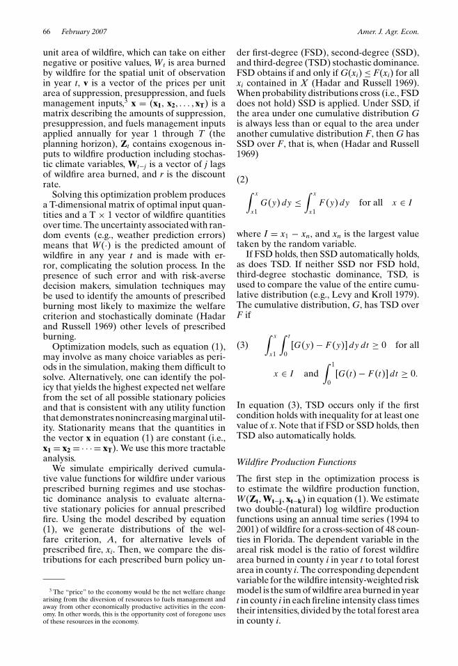
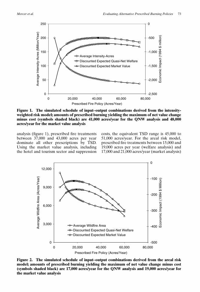
Results from the 100-year simulations of wild-fire under a range of prescribed burn policiesfor Volusia County are presented in figures 1(the intensity-weighted risk model) and 2 (theareal risk model). Each figure depicts boththe market value and QNW economic im-pacts associated with a range of stationaryprescribed burn policies. The welfare valuesare based on predicted impacts on the timberand housing sectors, while the market valuecurves use market values for the timber andhousing sectors, suppression costs, and changesin expenditures in the travel and hotel sec-tor. The models perform as expected, with in-creasing amounts of prescribed fire leading tolower area burned and intensity-weighted area

72 February 2007 Amer. J. Agr. Econ.

Table 3. Model Parameter Estimates of Fully Specified and Parsimonious Forms of Areal RiskFunctions

Full Model Parsimonious Model

Explanatory Variables Parameter Z-Value Parameter Z-Value

ln(Prescribed Burn Area/Forest Area) −0.262∗∗∗ −3.17 −0.284∗∗∗ −3.60ln(Prescribed Burn Areat−1 /Forest Area) −0.051 −0.46 — —ln(Prescribed Burn Areat−2 /Forest Area) −0.373∗∗∗ −3.32 −0.432∗∗∗ −3.61ln(Wildfire Areat−1 /Forest Area) −0.266∗∗∗ −4.73 −0.209∗∗∗ −4.28ln(Wildfire Areat−2 /Forest Area) −0.239∗∗∗ −4.42 −0.229∗∗∗ −4.61ln(Wildfire Areat−3 /Forest Area) −0.186∗∗∗ −3.62 −0.176∗∗∗ −3.34ln(Wildfire Areat−4 /Forest Area) −0.238∗∗∗ −3.77 −0.255∗∗∗ −4.49ln(Wildfire Areat−5 /Forest Area) −0.193∗∗∗ −3.12 −0.223∗∗∗ −3.87ln(Wildfire Areat−6 /Forest Area) −0.160∗∗∗ −2.78 −0.164∗∗∗ −3.21ln(Wildfire Areat−7 /Forest Area) −0.013 −0.21 — —ln(Wildfire Areat−8 /Forest Area) 0.066 0.99 — —ln(Wildfire Areat−9 /Forest Area) −0.149∗∗ −2.25 −0.153∗∗ −2.62ln(Wildfire Areat−10 /Forest Area) −0.197∗∗∗ −3.19 −0.149∗∗∗ −2.91ln(Wildfire Areat−11 /Forest Area) −0.104∗ −1.61 — —ln(Wildfire Areat−12 /Forest Area) −0.054 −0.93 — —ln(Pulpwood Harvestt−1 /Forest Area) 0.421∗∗ 2.29 — —ln(Pulpwood Harvestt−2 /Forest Area) 0.376∗ 1.89 — —ln(Pulpwood Harvestt−3 /Forest Area) −0.509∗∗∗ −2.97 −0.470∗∗∗ −3.77ln(Housing Density /Forest Area) 0.834 0.59 — —ENSO −0.312∗∗∗ −2.51 −0.262∗∗∗ −2.67NAO 0.934∗∗∗ 3.81 0.906∗∗∗ 4.101998 dummy 2.268∗∗∗ 8.22 2.310∗∗∗ 10.09

Number of cross sections 48 48Number of years 7 7Total panel observations 275 285Wald chi2 2,960 (prob > 1,645 (prob >

Chi2 = 0.000) Chi2 = 0.000)Log likelihood −228.0352 −276.6049

Notes: Single (∗), double (∗∗), and triple (∗∗∗) asterisk denote significance at 0.10, 0.05, and 0.01 levels, respectively. Dependent variables are natural logs of

each county’s annual total areal extent (acres) of wildfire (areal risk model) and the natural logs of sum of area burned (acres) at each intensity level times

the intensity level per county per year. Equation estimates reported here exclude estimates of 48 county dummies.

burned and lower overall net economic lossesand costs. Greater amounts of prescribed firelead to rising per-unit prescribed fire costs andmarginally smaller gains in damages averted.Together these produce the inverse-U shapedQNW curves in figures 1 and 2.

The intensity-weighted risk model predictsthat an annual rate of prescribed fire of 41,000acres (welfare analysis) or 48,000 acres (mar-ket value analysis) would maximize discountednet value change minus costs.11 The additional

11 The optimal amount of fuel treatment for a county may alsodepend on how the treatments are allocated spatially. Althoughsome anecdotal evidence supports this, empirical evidence is notyet available to validate this claim. However, if it turns out tobe true, our approach may underestimate the damage-cost reduc-tions of prescribed fire, suggesting that higher rates of prescribedfire may be optimal. Nevertheless, we do not expect that explicitspatial analysis would substantially affect our results on optimallevels of aggregate treatments across a county. In this paper, weassume that the actions of managers in the historical data were

7,000 acres treated in the market analysis re-sults from accounting for expenditures on firesuppression and wildfire impacts on the hoteland tourism sector. Comparing figures 1 and2, the annual prescribed fire amount that max-imizes QNW is about 33% lower in the arealrisk model than in the intensity-weighted riskmodel, regardless of which damage measuresare used. Although the stochastic dominanceanalyses fail to identify specific policy solu-tions, they do provide a range of treatmentsthat dominate all other policies tested. Usingthe intensity-weighted risk model and welfare

optimal, in the sense that prospective areas to burn were identifiedspatially and then prioritized (burned first) with an (constrained)economic optimization model in mind. When the budget or insti-tutional constraints are removed, we expect landowners to use thesame criteria for locating treatments on the landscape. Consistentwith our log–log model parameter estimates, the marginal effect ofeach additional acre prescribed burned declines with the absolutelevel of prescribed burn area in the county.

Mercer et al. Evaluating Alternative Prescribed Burning Policies 73

0

50

100

150

200

250

0 20,000 40,000 60,000 80,000

Prescribed Fire Policy (Acres/Year)

Avera

ge Inte

nsity-A

cre

s (

Mill

ion/Y

ear)

-2,500

-2,000

-1,500

-1,000

-500

0

Econom

ic Im

pact (1

994 $

mill

ion)

Average Intensity-Acres

Discounted Expected Quasi-Net Welfare

Discounted Expected Market Value

Figure 1. The simulated schedule of input–output combinations derived from the intensity-weighted risk model; amounts of prescribed burning yielding the maximum of net value changeminus cost (symbols shaded black) are 41,000 acres/year for the QNW analysis and 48,000acres/year for the market value analysis

analysis (figure 1), prescribed fire treatmentsbetween 37,000 and 43,000 acres per yeardominate all other prescriptions by TSD.Using the market value analysis, includingthe hotel and tourism sector and suppression

0

3,000

6,000

9,000

12,000

0 20,000 40,000 60,000 80,000

Prescribed Fire Policy (Acres/Year)

Ave

rag

e W

ildfire

Are

a (

Acre

s/Y

ea

r)

-500

-400

-300

-200

-100

0E

co

no

mic

Im

pa

ct

(19

94

$ M

illio

n)

Average Wildfire Area

Discounted Expected Quasi-Net Welfare

Discounted Expected Market Value

Figure 2. The simulated schedule of input–output combinations derived from the areal riskmodel; amounts of prescribed burning yielding the maximum of net value change minus cost(symbols shaded black) are 17,000 acres/year for the QNW analysis and 19,000 acres/year forthe market value analysis

costs, the equivalent TSD range is 45,000 to51,000 acres/year. For the areal risk model,prescribed fire treatments between 15,000 and19,000 acres per year (welfare analysis) and17,000 and 21,000 acres/year (market analysis)

74 February 2007 Amer. J. Agr. Econ.

dominate all other prescriptions by TSD.Both the discounted QNW and market valueanalyses produce maxima in the middle of theranges identified by the stochastic dominanceanalysis.

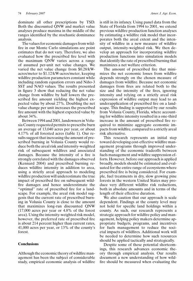
The values for economic damages from wild-fire in our Monte Carlo simulations are pointestimates that do not vary. Therefore, we alsoevaluated how the prescribed fire level withthe maximum QNW varies across a rangeof assumed per-unit net value changes. Wevaried the net value change from $0.28/kW-acres/meter to $1.12/kW-acres/meter, keepingwildfire production parameters constant whileincluding random equation errors and Nino-3SST and NAO values. The results presentedin figure 3 show that reducing the net valuechange from wildfire by half lowers the pre-scribed fire amount yielding the highest ex-pected value by about 27%. Doubling the netvalue change per unit increases the prescribedfire amount with the highest expected value byabout 34%.

Between 1994 and 2001, landowners in Volu-sia County requested permits to prescribe burnan average of 13,040 acres per year, or about4.17% of all forested acres (table 1). Our re-sults suggest that increasing the amount of pre-scribed burning in Volusia County would re-duce both the areal risk and intensity-weightedrisk of subsequent wildfires and associateddamages. Because the intensity of a fire isstrongly correlated with the damages observed(Kennard 2004) and prescribed burning re-duces wildfire intensity in addition to area,using a strictly areal approach to modelingwildfire production will underestimate the trueimpact of prescribed fire on subsequent wild-fire damages and hence underestimate the“optimal” rate of prescribed fire for a land-scape. For example, the areal risk model sug-gests that the current rate of prescribed burn-ing in Volusia County is close to the amountthat maximizes long-run discounted QNW(17,000 acres per year or 4.8% of the forestarea). Using the intensity-weighted risk model,however, the preferred rate of prescribed fireis about 214 percent higher than current rates,41,000 acres per year, or 13% of the county’sforest.

Conclusions

Although the economic theory of wildfire man-agement has been the subject of considerablestudy, empirical economic analysis of wildfire

is still in its infancy. Using panel data from theState of Florida from 1994 to 2001, we extendprevious wildfire production function analysesby estimating a wildfire risk model that incor-porates both the areal extent and the inten-sity of wildfire in a new measure of wildfireoutput, intensity-weighted risk. We then de-velop an approach for incorporating wildfireproduction functions into simulation modelsthat identify the rate of prescribed burning thatmaximizes a net welfare criterion.

The amount of prescribed fire that mini-mizes the net economic losses from wildfiredepends strongly on the chosen measure ofdamages from wildfire. Because net economicdamages from fires are related both to thesize and the intensity of the fires, ignoringintensity and relying on a strictly areal riskexpression of wildfire output may lead to anunderapplication of prescribed fire on a land-scape. This finding is supported by our resultsfrom Volusia County, Florida, where account-ing for wildfire intensity resulted in a one-thirdincrease in the amount of prescribed fire re-quired to minimize aggregate economic im-pacts from wildfire, compared to a strictly arealrisk alternative.

This research represents an initial steptoward developing cost-effective wildfire man-agement programs through improved under-standing of the economic tradeoffs betweenfuels management and wildfire suppression ef-forts. However, before our approach is appliedbroadly, models should be estimated and eval-uated for the entire range of ecosystems whereprescribed fire is being considered. For exam-ple, fuel treatments in dry, slow growing pineforests in the western United States may pro-duce very different wildfire risk reductions,both in absolute amounts and in terms of thelength of their effective duration.

We also caution that our approach is scaledependent. Findings at the county level maynot hold for specific land holdings within acounty. As such, our research represents astrategic approach for wildfire policy and man-agement, helping policy makers determine ap-propriate budgets, programs, and incentivesfor fuels management to reduce the soci-etal impacts of wildfires. Additional work willbe needed to determine how such resourcesshould be applied tactically and strategically.

Despite some of these potential shortcom-ings, this research advances economic the-ory through empirical analysis. Our resultsdocument a new understanding of how wild-fire should be measured when evaluating the

Mercer et al. Evaluating Alternative Prescribed Burning Policies 75

Prescribed Burn at Maximum (Acres/Year)

0

10,000

20,000

30,000

40,000

50,000

60,000

70,000

0.00 0.20 0.40 0.60 0.80 1.00 1.20

Damages ($/Kilowatt-Acre/Meter)

Pre

scrib

ed

Fire

Po

licy (

Acre

s/Y

ea

r)

Actual Damages

per Unit Are Half

Actual Damages per

Unit Are Double Assumed

Damages per Unit

Figure 3. Simulated schedule of prescribed fire policies yielding the highest expected values,identified by varying assumed wildfire damages per unit, using the intensity-weighted risk modeland quasi-net welfare losses from wildfire

efficacy of wildfire management inputs. Ourresults suggest that wildfire prevention andmanagement activities have an effect on dam-ages that exceed those reflected in simple mea-sures of area burned. Additionally, our find-ing that the national supply of prescribed fireservices responds inelastically to price shouldbe a warning that the cost of prescribed fireservices may increase rapidly with expandedprescribed fire use in the United States. Ourestimated prescribed fire supply function im-plies that if programs like the President’sHealthy Forests Initiative succeed in increas-ing contracts for prescribed fire on public lands,private landowners may face higher costs forsimilar services. Therefore, an unintended con-sequence of expanded use of fuel treatmentson public lands may be a reduction in pre-scribed fire on private lands.

Our research suggests the need for addi-tional research in several areas. First, a bet-ter understanding of the supply of prescribedfire services would allow more realistic simu-lations of nonmarginal changes in prescribedfire inputs. Second, identification of the en-velope of economically optimal levels of anyparticular input needs to account for substi-tutability across inputs. Mechanical fuel treat-ments may interact with prescribed burning,such that the “best” prescribed fire levels iden-tified without such interactions may differ fromthose found when other approaches are in-cluded in estimating optimal combinations of

treatments. Similar cautions exist with respectto fire suppression. It is possible that fire sup-pression resource efficiencies may be changedby fuels management, but data limitations pre-cluded identification of such changes. Finally,both wildfire and prescribed fire provide a suiteof public and private goods and bads that gobeyond the economic damages and marketprices of direct inputs described in this study.Although considerable research is needed toquantify the values of these nonmarket im-pacts of wildfire, including these other valuesin optimization models could lead to a moreaccurate assessment of public and private pol-icy choices for wildfire management.

[Received June 2004;accepted April 2006.]

References

Aplet, G.H., and B. Wilmer. 2003. The Wildland FireChallenge: Focus on Reliable Data, CommunityProtection, and Ecological Restoration. Ecol-

ogy and Economics Research Department.

Washington DC: The Wilderness Society.

Barnett, T.P., and J. Brenner. 1992. “Prediction of

Wildfire Activity in the Southeastern United

States.” Southeast Regional Climate Center Re-search Paper Number 011592. Columbia, SC:

South Carolina Water Resources Commission.

Bell, E., D. Cleaves, H. Croft, S. Husari, and E.

Schuster. 1995. Fire Economics Assessment

76 February 2007 Amer. J. Agr. Econ.

Report. U.S. Department of Agriculture For-

est Service Report to Fire and Aviation

Management.

Bellinger, M.D., H.F. Kaiser, and H.A. Harrison.

1983. “Economic Efficiency of Fire Manage-

ment on Nonfederal Forest and Range Lands.”

Journal of Forestry 81:373–5.

Blackley, D.M. 1999. “The Long-Run Elasticity of

New Housing Supply in the United States: Em-

pirical Evidence for 1950 to 1994.” Journal ofReal Estate Finance and Economics 18:25–42.

Brenner, J. 1991. “Southern Oscillation Anomalies

and their Relation to Florida Wildfires.” FireManagement Notes 52:28–32.

Brockway, D., and K.W. Outcalt. 2000. “Restor-

ing Longleaf Pine Wiregrass Ecosystems: Hex-

azinone Application Enhances Effects of Pre-

scribed Fire.” Forest Ecology and Management137:121–38.

Brose, P., and D. Wade. 2002. “Potential Fire Behav-

ior in Pine Flatwood Forests following Three

Different Fuel Reduction Techniques.” ForestEcology and Management 163:71–84.

Butry, D.T., D.E. Mercer, J.P. Prestemon, J.M. Pye,

and T.P. Holmes. 2001. “What Is the Price

of Catastrophic Wildfire?” Journal of Forestry99:9–17.

Byram, G.M. 1959. “Chapter 3: Combustion of For-

est Fuels.” In K.P. Davis, ed. Forest Fire Con-trol and Use. New York: McGraw-Hill, pp. 61–

89.

Cleaves, D.A., and J.D. Brodie. 1990. “Economic

Analysis of Prescribed Burning.” In J.D. Wal-

stad, S.R. Radosevich, and D.V. Sandberg, eds.

Natural and Prescribed Fire in Pacific North-west Forests. Corvallis, OR: Oregon State Uni-

versity Press, pp. 271–82.

Cleaves, D.A., J. Martinez, and T.K. Haines. 2000.

“Influences of Prescribed Burning Activity and

Costs in the National Forest System.” U.S. De-

partment of Agriculture Forest Service, Gen.

Tech. Rpt. SRS-37.

Davis, L.S. 1965. The Economics of Wildfire Pro-tection with Emphasis on Fuel Break Sys-tems. Sacramento, CA: California Division of

Forestry.

Davis, L.S., and R.W. Cooper. 1963. “How Pre-

scribed Burning Affects Wildfire Occurrence.”

Journal of Forestry 61:915–17.

Donovan, G.H., and D.B. Rideout. 2003. “A Refor-

mulation of the Cost Plus Net Value Change

(C+NVC) Model of Wildfire Economics.” For-est Science 49:318–23.

Florida Bureau of Economic and Business Re-

search. 2002. Long-term Economic Forecast2001, Vol. 1 and 2 (CD-ROM). University of

Florida, Gainesville, FL.

Florida Department of Agriculture and Consumer

Services. 2005. “Wildland Fire: Prescribed

Fire.” Florida Division of Forestry. Avail-

able at http://www.fl-dof.com/wildfire/rx index.

html, accessed 11 July 2005.

Gamache, A.E. 1969. “Development of a Method

for Determining the Optimum Level of For-

est Fire Suppression Manpower on a Sea-

sonal Basis.” PhD dissertation, University of

Washington.

Gonzalez-Caban, A., and C.W. McKetta. 1986. “An-

alyzing Fuel Treatment Costs.” Western Journalof Applied Forestry 1:116–21.

Gorte, J.K., and R.W. Gorte. 1979. Application ofEconomic Techniques to Fire Management—A Status Review and Evaluation. Ogden, UT:

USDA Forest Service, Gen. Tech. Rpt. INT-53.

Hadar, J., and W.R. Russell. 1969. “Rules for Order-

ing Uncertain Prospects.” American EconomicReview 59:25–34.

Haines, T.K., and D.A. Cleaves. 1999. “The Legal

Environment for Forestry Prescribed Burning

in the South: Regulatory Programs and Volun-

tary Guidelines.” Southern Journal of AppliedForestry 23:170–74.

Headly, R. 1916. Fire Suppression District 5. Wash-

ington DC: USDA Forest Service.

Hesseln, H. 2000. “The Economics of Prescribed

Burning: A Research Review.” Forest Science46:332–4.

Kennard, D.K. 2004. “Depth of Burn.” For-est Encyclopedia. Available at http://www.

forestencyclopedia.net, accessed 15 January

2004.

Koehler, J.T. 1992–93. “Prescribed Burning: A Wild-

fire Prevention Tool?” Fire Management Notes53–54:9–13.

Krinsky, I., and A.L. Robb. 1986. “On Approximat-

ing the Statistical Properties of Elasticities.”

Review of Economics and Statistics 68:715–19.

Levy, H., and Y. Kroll. 1979. “Efficiency Analy-

sis with Borrowing and Lending: Criteria and

Their Effectiveness.” Review of Economics andStatistics 61:125–30.

Lovejoy, P.S. 1916. “Costs and Values of Forest Pro-

tection.” Forestry Quarterly 14(1):24–38.

Martin, G.C. 1988. “Fuels Treatment Assessment—

1985 Fire Season in Region 8.” Fire Manage-ment Notes 49:21–24.

Mills, T.J., and F.W. Bratten. 1982. FEES: Designof a Fire Economics Evaluation System. Berke-

ley, CA: USDA Forest Service, Gen. Tech. Rpt.

PSW-65.

Mutch, R.E. 2002. “Fire Situation in the United

States.” International Forest Fire News 27:6–13.

National Oceanic and Atmospheric Adminis-

tration. 2003a. “Monthly Atmospheric and

Mercer et al. Evaluating Alternative Prescribed Burning Policies 77

SST Indices.” Available at http://www.cpc.

noaa.gov/data/indices/sstoi.indices, accessed

11 April 2003.

——. 2003b. “Standardized Northern Hemisphere

Teleconnection Indices.” Available at ftp://ftp.

ncep.noaa.gov/pub/cpc/wd52dg/data/indices/

tele index.nh, accessed 11 April 2003.

National Wildfire Coordinating Group. 1996. Glos-sary of Wildland Fire Terminology. NFES Re-

port #1832. National Interagency Fire Center,

Boise, Idaho.

Outcalt, K.W., and D.D. Wade. 2004. “Fuels Man-

agement Reduces Tree Mortality from Wild-

fires in Southeastern United States.” SouthernJournal of Applied Forestry 28:28–34.

Prestemon, J.P., J.M. Pye, D.T. Butry, T.P. Holmes,

and D.E. Mercer. 2002. “Understanding Broad

Scale Wildfire Risks in a Human-Dominated

Landscape.” Forest Science 48:685–93.

Rideout, D.B., and P.N. Omi. 1990. “Alternate Ex-

pressions for the Economic Theory of Forest

Fire Management.” Forest Science 36:614–24.

——. 1995. “Estimating the Cost of Fuels Treat-

ment.” Forest Science 41:664–74.

Samuelson, P.A. 1954. “The Pure Theory of Pub-

lic Expenditures.” Review of Economics andStatistics 36:387–9.

——. 1955. “Diagrammatic Exposition of a Theory

of Public Expenditures.” Review of Economicsand Statistics 37:350–56.

Sparhawk, W.N. 1925. “The Use of Liability Ratings

in Planning Forest Fire Protection.” Journal ofAgricultural Research 30:693–762.

Stephens, S.L. 1997. “Evaluation of the Effects of

Silvicultural and Fuels Treatments on Poten-

tial Fire Behaviour in Sierra Nevada Mixed-

Conifer Forests.” Forest Ecology and Manage-ment 105:21–35.

Teeter, L.D., and A.A. Dyer. 1986. “A Multiat-

tribute Utility Model for Incorporating Risk

in Fire Management Planning.” Forest Science32:1032–48.

The White House. 2002. Healthy Forests: AnInitiative for Wildfire Prevention and StrongerCommunities. Washington DC: Office of

the President of the United States. Avail-

able at http://www.whitehouse.gov/infocus/

healthyforests/toc.html, accessed 4 February

2004.

USDA Forest Service. 2000. Managing the Impactof Wildfires on Communities and the Environ-ment: A Report to the President in Response tothe Wildfires of 2000. Washington DC.

——. 2004. Strategic Plan for Fiscal Years 2004–2008. Final Report. Washington DC.

USDI/USDA. 1995. Federal Wildland Fire Manage-ment Policy and Program Review Report. U.S.

Department of the Interior, U.S. Department

of Agriculture. Washington DC.

Wade, D.D., and J.D. Lunsford. 1988. A Guide forPrescribed Fire in Southern Forests. Atlanta:

USDA Forest Service, Southern Region Tech-

nical Publication R8-TP 11.

Wagle, R.F., and T.W. Eakle. 1979. “A Controlled

Burn Reduces the Impact of a Subsequent

Wildfire in a Ponderosa Pine Vegetation Type.”

Forest Science 25:123–29.

Westerling, A.L., T.J. Brown, A. Gershunov, D.R.

Cayan, and M.D. Dettinger. 2002. “Climate and

Wildfire in the Western United States.” Bul-letin American Meteorological Society 84:595–

604.

Woodruff, S.D., R.J. Slutz, R.L. Jenne, and P.M.

Steurer. 1987. “A Comprehensive Ocean-

Atmosphere Data Set.” Bulletin of theAmerican Meteorological Society 68:1239–

50.

Yoder, J., M. Tilley, D. Engle, and S. Fuhlendorf.

2003. “Economics and Prescribed Fire Law in

the United States.” Review of Agricultural Eco-nomics 25:218–33.

Zabel, J.E. 2004. “The Demand for Housing Ser-

vices.” Journal of Housing Economics 13:16–

35.