Evaluating China's integration in world trade with a gravity model

ISSN 1561081-0

9 7 7 1 5 6 1 0 8 1 0 0 5

WORKING PAPER SER IESNO 693 / NOVEMBER 2006

EVALUATING CHINA’S INTEGRATION IN WORLD TRADE WITH A GRAVITY MODEL BASED BENCHMARK

and Bernd Schnatzby Matthieu Bussière

In 2006 all ECB publications

feature a motif taken

from the €5 banknote.

WORK ING PAPER SER IE SNO 693 / NOVEMBER 2006

This paper can be downloaded without charge from http://www.ecb.int or from the Social Science Research Network

electronic library at http://ssrn.com/abstract_id=942730

1 We have benefited from very valuable comments during the Far Eastern Meeting of the Econometric Society in Beijing in July 2006, the 10th International Conference on Macroeconomic Analysis and International Finance in Rethymno in May 2006, the Conference on “Globalisation and Regionalism” in Sydney in December 2005 and at the European Central Bank in June 2005, especially from our discussants K.-K. Tang and Mardi Dungey. We also would like to thank for their useful advice Mike Artis, Richard Baldwin, Anindya

Banerjee, Agnès Bénassy-Quéré, Jarko Fidrmuc, Peter Egger, Françoise Lemoine, Warwick McKibbin, Adrian Pagan and Alvaro Santos-Rivera. The views expressed in this paper are those of the authors and do not necessarily represent those of the European Central Bank.

2 European Central Bank, Kaiserstrasse 29, 60311 Frankfurt am Main, Germany; e-mails: [email protected]; [email protected]

EVALUATING CHINA’S INTEGRATION IN WORLD TRADE WITH A GRAVITY

MODEL BASED BENCHMARK 1

by Matthieu Bussière 2

and Bernd Schnatz 2

© European Central Bank, 2006

AddressKaiserstrasse 2960311 Frankfurt am Main, Germany

Postal addressPostfach 16 03 1960066 Frankfurt am Main, Germany

Telephone+49 69 1344 0

Internethttp://www.ecb.int

Fax+49 69 1344 6000

Telex411 144 ecb d

All rights reserved.

Any reproduction, publication andreprint in the form of a differentpublication, whether printed orproduced electronically, in whole or inpart, is permitted only with the explicitwritten authorisation of the ECB or theauthor(s).

The views expressed in this paper do notnecessarily reflect those of the EuropeanCentral Bank.

The statement of purpose for the ECBWorking Paper Series is available fromthe ECB website, http://www.ecb.int.

ISSN 1561-0810 (print)ISSN 1725-2806 (online)

3ECB

Working Paper Series No 693November 2006

CONTENTS

Abstract 4

Non-technical summary 51. Introduction 6

2. Bilateral trade flows: stylised facts 8

3. Estimating the model 13

3.1. Gravity fundamentals 13

3.2. Methodological aspects 14

3.3. Specification 15

3.5. Estimation results 17

4. Extracting information from thepredicted values 19

4.1. Results from the first-stage regression 19

4.2 Results from the second stage regression:extracting information fromcountry-heterogeneity 21

5. Conclusions 26

References 28

Data Sources 31

Chart appendix 32

Table appendix 37European Central Bank Working Paper Series 39

3.4. Data 16

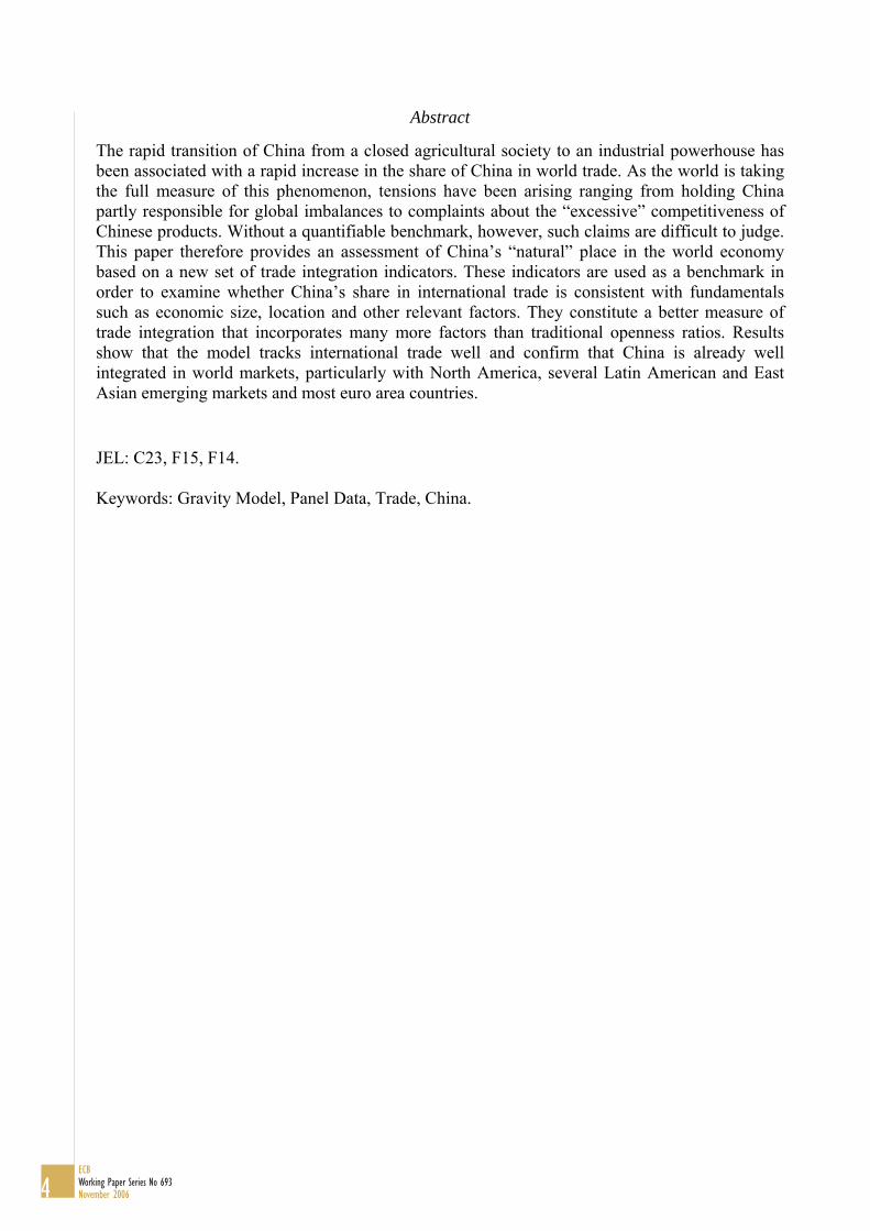
Abstract

been associated with a rapid increase in the share of China in world trade. As the world is taking the full measure of this phenomenon, tensions have been arising ranging from holding China partly responsible for global imbalances to complaints about the “excessive” competitiveness of Chinese products. Without a quantifiable benchmark, however, such claims are difficult to judge. This paper therefore provides an assessment of China’s “natural” place in the world economy based on a new set of trade integration indicators. These indicators are used as a benchmark in

such as economic size, location and other relevant factors. They constitute a better measure of trade integration that incorporates many more factors than traditional openness ratios. Results show that the model tracks international trade well and confirm that China is already well integrated in world markets, particularly with North America, several Latin American and East Asian emerging markets and most euro area countries. JEL: C23, F15, F14. Keywords: Gravity Model, Panel Data, Trade, China.

The rapid transition of China from a closed agricultural society to an industrial powerhouse has

order to examine whether China’s share in international trade is consistent with fundamentals

4ECBWorking Paper Series No 693November 2006

Non-technical summary

China’s reform process towards a market-based economy has triggered a significant reorientation of international trade flows. China has indeed experienced very quick trade integration into world markets as exemplified by a strong increase in its share in world trade. As the world is taking the full measure of this phenomenon, tensions have emerged in the political and economic sphere. In particular, the emergence of China was perceived to affect the competitiveness and the employment situation in mature economies. Without a quantifiable benchmark, such claims are difficult to judge; however, to our knowledge, such quantification has never been attempted.

The aim of the present paper is to fill in this gap and to contribute to the policy debate by providing an empirical assessment of China’s “natural” place in the world economy. Building on a companion study (see Bussière, Fidrmuc and Schnatz (2005)), we use a gravity model to shed light on the overall degree of trade intensity of a large number of countries as well as the depth of bilateral trade linkages of China with major economies. Our gravity model employs a very large dataset of bilateral trade flows including more than sixty trading partners over more than twenty years. In the standard regression this amounts to more than 3,500 bilateral trade relationships and almost 53,000 observations. The model is estimated in a two-step panel data framework – as advocated by Cheng and Wall (2005) – which takes country heterogeneity properly into account. The estimates are plausible and robust to different estimators and samples. Moreover, they are able to capture most of the variation in bilateral trade flows, both across countries and over time. The new measure of multilateral trade integration is based on the part of the fixed effects which are orthogonal to available time-invariant variables in the second step regression. It constitutes a better measure of trade integration than standard variables such as the share in world trade or the ratio of exports and imports to GDP, because it incorporates many more factors. Accordingly, it is more appropriate as a benchmark for examining whether China’s share in international trade is consistent with economic fundamentals.

The paper suggests that the rise in trade flows between China and its trading partners should not, per se, come as a surprise. China's shift towards more market-oriented policies together with robust economic growth was instrumental for the reorientation and deepening of trade linkages. At the same time, we find that China – given its size and location – is already well integrated into the world economy, which contrasts with the experience of other transition countries with a planned-economy history in Central and Eastern Europe. In more detail, the new indicators of trade intensity suggest that China displays a higher degree of global trade integration than many other industrialised countries or Asian trading partners. However, our measure of trade integration for China is not higher than that of several developed countries such as the US, Germany or Japan. Our bilateral measure of trade integration suggests that China seems to be particularly well integrated with the United States and Canada, several Latin American and East Asian countries as well as most euro area countries.

5ECB


1. Introduction Famously, Napoleon is said to have remarked that “China is a sickly, sleeping giant. But when she awakes the world will tremble”. Nearly two centuries later, China is truly awake and it seems that the world is now taking the full measure of this phenomenon: the brisk pace of China’s integration into the world economy strikingly affected global trade, while it is also perceived to have triggered tensions in the political and economic sphere. These tensions range from holding China partly responsible for global imbalances to complaints about the “excessive” competitiveness of Chinese products adversely affecting the employment situation in partner countries.

Without a quantifiable benchmark, however, such claims appear very difficult to assess. Historically, the rise of China may essentially constitute a return of the country to where it once was before it fell asleep. For several hundred years, China was a rich empire and highly advanced in terms of technology, albeit relatively closed to the rest of the world – as symbolised by the Great Wall of China encircling almost 4,000 miles of their land.2 This relative isolation lasted until the early 19th century, when China still accounted for about one third of world output. Thereafter, the country experienced a long period of economic stagnation and even decline in the 1950s and 1960s. Following the rapid transition of China from an impoverished and closed agricultural society to a globally integrated industrial powerhouse, the penetration of world trade by Chinese products could be rationalised at least partly by the quickly growing size of its economy and by its opening up towards the world economy which culminated in its WTO accession in 2001.3 Unless China were to develop as an autarky, which no one would seriously consider, one can expect that China is going to take up some share of world trade. The question then is: how much?

This raises the question of the “natural” place of China in the world economy and calls for a quantification of China’s share in international trade, given its economic size, location and other relevant fundamentals. However, to our knowledge, such exercise has never been attempted. The aim of the present paper is to fill in this gap by using results from a gravity model to derive a measure of multilateral trade integration (China against all trading partners) but also of bilateral trade integration (between China and each of its trading partners). Gravity models previously applied to China had a different focus as they commonly aimed at quantifying the impact of policy variables, whereas our aim is to develop a new set of trade integration indicators which are used as a benchmark to examine whether the China’s external trade is consistent with the economic fundamentals included in a gravity equation. For instance, Abraham and Van Hove

2 China has been at times very open to the world, like in the early 15th century under Emperor Yung Ho, who

considerably developed the naval and merchant fleet and opened new trade routes going as far as the Eastern coast of Africa; see Boorstin (1983) for a historical perspective.

3 See Branstetter and Lardy (2006) for a very detailed and comprehensive overview of the major steps in the evolution of Chinese policy towards international economic integration.


(2005) use a gravity model mainly for Asian countries in the 1990s to investigate the impact of regional free trade arrangements on China’s trade. Likewise, Lee and Park (2005) use the large panel of Glick and Rose (2003) – more than 200,000 country pairs – to study the trade diverting and trade creating effects of free trade arrangements. Using a smaller panel, Bénassy-Quéré and Lahrèche-Révil (2003) examine the impact of a yuan revaluation. Meanwhile, Eichengreen, Rhee and Tong (2004) investigate the effect of China’s rapid trade integration for other Asian economies given their structure of external trade. They find that Chinese exports tend to crowd out exports from other Asian economies, especially for consumer goods. Filippini, Molini and Pozzoli (2005) decompose trade into three categories of technological content and test whether a measure of “technological distance” helps explaining bilateral trade flows. Closer to our approach, Batra (2004) estimates a gravity model with a focus on India using a cross-section equation and finds that India has significant scope for strengthening trade with China and the rest of Asia.4

Our approach differs from the existing literature as we use the results of a gravity model as a benchmark for China’s trade integration instead of testing for a particular theory or evaluating the impact of a given policy variable. Building on a companion study (see Bussière, Fidrmuc and Schnatz (2005), our gravity model is based on a very large dataset of bilateral trade flows including more than sixty trading partners over more than twenty years, which is able to capture most of the variation in bilateral trade flows, both across countries and over time. We consider only trade in goods since a breakdown of trade in services by partner country is not available for all countries in the sample. The model is estimated in a two-step panel data framework – as advocated by Cheng and Wall (2005) – which takes country heterogeneity properly into account. The chosen empirical method allows constructing an indicator which is used as a benchmark for comparing trade intensity across countries. These indicators should, however, not be given a normative interpretation, as they may depend on a variety of factors such as political configurations or the commodity composition of trade flows between a particular pair of countries.

The information provided by these indicators suggests that (i) China is already very well integrated in world markets and (ii) that the strong rise of Chinese trade flows with major industrial countries in the 1990s and early 2000s is well explained by the gravity fundamentals.5 Both results are noticeable as they contrast with the experience of other transition countries with a planned-economy history in Central and Eastern Europe, as analysed in Bussière, Fidrmuc and Schnatz (2005). Indeed, these countries were found to have experienced a long period during which their trade flows were below the gravity benchmark, after the beginning of the transition process. Accordingly, we also found that actual trade grew more strongly than projected trade for

4 This review does not include the studies that took a completely different approach to China’s trade integration

and have used general equilibrium models instead; see McKibbin and Woo (2002), Yang (2003), or Prasad (2004) for a review.

5 It seems however that the model underpredicts the acceleration of China’s trade flows after 2003.

7ECB


these countries, which we mainly interpreted as a convergence towards their trade potential. We offer several possible interpretations of this difference in Section 4; they relate to the role of process trade, foreign investment, the Chinese diaspora, as well as the role of the war for some South Eastern European countries. Meanwhile, the indicators of trade intensity suggest that China displays a higher degree of global trade integration than many other industrialised countries or Asian trading partners. However, our measure of trade integration for China is not higher than that of several developed countries such as Germany, the US, or Japan.

Turning to our bilateral measure of trade integration (i.e., using the overall trade integration of each partner countries as a benchmark), China appears to be well integrated with Canada, Australia, the United States and several Latin American and East Asian emerging markets. However, if compared with the trade intensity of these countries with other Asian economies, trade intensity between China and the United States or Australia does not seem to be exceptional. On the other side of the spectrum, many Central and Eastern European countries have less intense trade links with China. Moreover, China’s trade intensity with India is found to be very low, which could be reconciled with historical developments. Among euro area countries, Germany, France and Spain seem to be well integrated with China already.

The rest of the paper is organised as follows: section 2 shows some of the key stylised facts that motivated the choice of our specification; section 3 presents the gravity equation and the regression results, section 4 reports the results for selected country-pair examples and focuses on the information extracted from the second stage regression (the trade integration indicators). The last section concludes.

2. Bilateral trade flows: stylised facts In order to better grasp the nature of China’s integration in world markets, Table 1 presents five indicators of trade integration for China and other selected economies in 1995 and 2005 (more detailed information on the trade shares of selected economies going back to the 1980s can be found in the Chart Appendix). Four key insights can be derived from Table 1.

First, over the past ten years, the share of China in world trade has more than doubled, from 3.7% to 7.7%, which is by far the largest increase recorded in the table.6 Accordingly, China has become the third largest trading partner in the world, behind the euro area and the US.7 This reflects both the buoyant economic growth recorded in China over this period and the rising

6 China did not only record by far the largest increase in absolute terms. What is even more noticeable is that it

also recorded the largest increased in relative terms (by 108%), second only to Bosnia (see Table 3 in the appendix), whose share rose by nearly 300% mainly reflecting its very small share in 1995.

7 For a meaningful comparison across countries, Table 1 reports the share of extra-euro area trade. The share of total (intra- plus extra-) euro area trade would be much higher as it includes trade across euro area countries (representing a little bit more than half of total trade). Detailed account and analysis of euro area trade can be found in Anderton, di Mauro and Moneta (2004).


integration of China into the global economy. As to the first factor, China’s share in world GDP rose from 9.5% to 15.4% between 1995 and 2005 (at purchasing power parity levels).8 As to the second factor, China’s openness ratio – measured as the sum of imports and exports to GDP – doubled from around 33% to over 62% between 1995 and 2005 (see Table 1, col (f) and (g)). China is therefore, according to this measure, almost as open as Germany (64%) and more open than the United Kingdom (40%) or the United States (20%). The increase in China’s trade ratio was not linear: it remained broadly constant at around 32% between 1995 and 1999. Subsequently, it rose to about 38% in 2000 and 2001 to reach nearly 42% in 2002. Thereafter, it experienced a first jump to above 50% in 2003 and to more than 58% in 2004. To anticipate on the results, our model is able to account for the strong rise until 2002 but underpredicts the strong acceleration that took place in 2003.

A second striking feature of China’s integration into world markets is that the composition of China’s trade flows by trading partners has remained broadly stable over this period. China’s external trade is concentrated among four main regions: Emerging Asia, the euro area, the United States and Japan (see Table 1, col. (b) and (c)). Mainly reflecting their geographical proximity, the other emerging Asian countries constitute the most important trading partner of China, accounting for 26.5% of Chinese trade. Among these countries, Hong Kong and South Korea are the most important trading partners, followed by Singapore and Malaysia.9 The close trade ties with the latter two countries might also be partly attributable to the share of the population of Chinese origin in these countries. Beyond emerging Asia, the United States is the single most important trading partner followed by Japan and the euro area. Each of these countries/regions accounts for 12% to 15% of China’s trade. While the share of most major countries and regions was broadly stable in 2005 compared to 1995, the share of Japanese goods in Chinese trade has declined significantly.10 Among the euro area countries, Germany is the most important trading partner of China, mainly reflecting the economic size of Germany as compared to other countries in the region.

8 This measure uses GDP evaluated in PPP terms, i.e. converting the GDP of all countries using Purchasing Power

Parity exchange rates. In nominal (US dollar) terms, China’s share also doubled but at a lower level from 2.5% to 5% of world GDP over this period, as the yuan’s current exchange rate is generally found to be lower than its PPP exchange rate, which partly reflects China’s stage of economic development and the corresponding lower prices of non-traded goods in China. This may be further compounded if, as widely perceived, the Chinese currency is undervalued. Although this finding is often reported in the literature, the magnitude of the undervaluation varies considerably across studies, see for instance Chang and Shao (2004), Coudert and Couharde (2005) or Frankel (2005).

9 Bilateral trade data between China and Hong Kong partly reflect transit trade, see for instance Schindler and Beckett (2005) for a discussion.

10 As shown in the chart Appendix, the share of Japan has actually decreased for many countries in the world.

9ECB


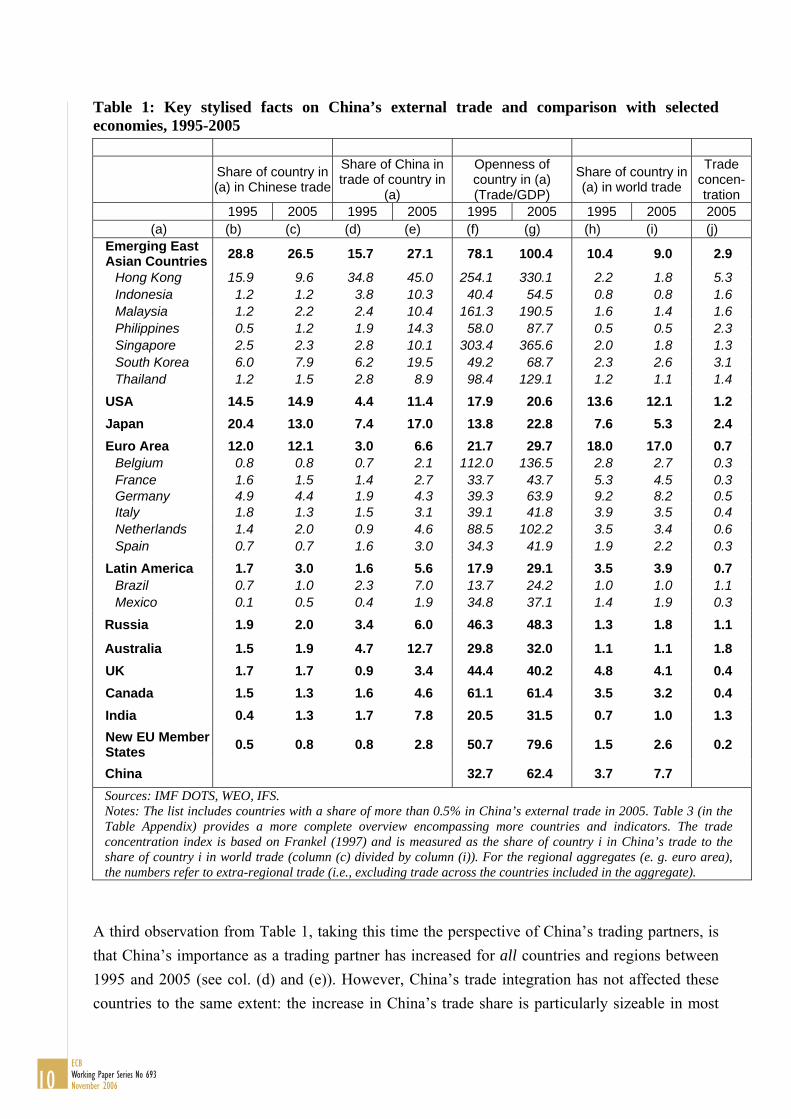
Table 1: Key stylised facts on China’s external trade and comparison with selected economies, 1995-2005

Share of country in (a) in Chinese trade

Share of China in trade of country in

(a)

Openness of country in (a) (Trade/GDP)

Share of country in (a) in world trade

Trade concen-tration

1995 2005 1995 2005 1995 2005 1995 2005 2005 (a) (b) (c) (d) (e) (f) (g) (h) (i) (j)

Emerging East Asian Countries 28.8 26.5 15.7 27.1 78.1 100.4 10.4 9.0 2.9

Hong Kong 15.9 9.6 34.8 45.0 254.1 330.1 2.2 1.8 5.3 Indonesia 1.2 1.2 3.8 10.3 40.4 54.5 0.8 0.8 1.6 Malaysia 1.2 2.2 2.4 10.4 161.3 190.5 1.6 1.4 1.6 Philippines 0.5 1.2 1.9 14.3 58.0 87.7 0.5 0.5 2.3 Singapore 2.5 2.3 2.8 10.1 303.4 365.6 2.0 1.8 1.3 South Korea 6.0 7.9 6.2 19.5 49.2 68.7 2.3 2.6 3.1 Thailand 1.2 1.5 2.8 8.9 98.4 129.1 1.2 1.1 1.4

USA 14.5 14.9 4.4 11.4 17.9 20.6 13.6 12.1 1.2 Japan 20.4 13.0 7.4 17.0 13.8 22.8 7.6 5.3 2.4 Euro Area 12.0 12.1 3.0 6.6 21.7 29.7 18.0 17.0 0.7

Belgium 0.8 0.8 0.7 2.1 112.0 136.5 2.8 2.7 0.3 France 1.6 1.5 1.4 2.7 33.7 43.7 5.3 4.5 0.3 Germany 4.9 4.4 1.9 4.3 39.3 63.9 9.2 8.2 0.5 Italy 1.8 1.3 1.5 3.1 39.1 41.8 3.9 3.5 0.4 Netherlands 1.4 2.0 0.9 4.6 88.5 102.2 3.5 3.4 0.6 Spain 0.7 0.7 1.6 3.0 34.3 41.9 1.9 2.2 0.3

Latin America 1.7 3.0 1.6 5.6 17.9 29.1 3.5 3.9 0.7 Brazil 0.7 1.0 2.3 7.0 13.7 24.2 1.0 1.0 1.1 Mexico 0.1 0.5 0.4 1.9 34.8 37.1 1.4 1.9 0.3

Russia 1.9 2.0 3.4 6.0 46.3 48.3 1.3 1.8 1.1 Australia 1.5 1.9 4.7 12.7 29.8 32.0 1.1 1.1 1.8 UK 1.7 1.7 0.9 3.4 44.4 40.2 4.8 4.1 0.4 Canada 1.5 1.3 1.6 4.6 61.1 61.4 3.5 3.2 0.4 India 0.4 1.3 1.7 7.8 20.5 31.5 0.7 1.0 1.3 New EU Member States 0.5 0.8 0.8 2.8 50.7 79.6 1.5 2.6 0.2

China 32.7 62.4 3.7 7.7 Sources: IMF DOTS, WEO, IFS. Notes: The list includes countries with a share of more than 0.5% in China’s external trade in 2005. Table 3 (in the Table Appendix) provides a more complete overview encompassing more countries and indicators. The trade concentration index is based on Frankel (1997) and is measured as the share of country i in China’s trade to the share of country i in world trade (column (c) divided by column (i)). For the regional aggregates (e. g. euro area), the numbers refer to extra-regional trade (i.e., excluding trade across the countries included in the aggregate).

A third observation from Table 1, taking this time the perspective of China’s trading partners, is that China’s importance as a trading partner has increased for all countries and regions between 1995 and 2005 (see col. (d) and (e)). However, China’s trade integration has not affected these countries to the same extent: the increase in China’s trade share is particularly sizeable in most


other emerging Asian economies, Japan, Australia and the United States, while it is still more moderate in other regions.

Notwithstanding the comparatively modest weight of China in euro area trade, it is noticeable that the share of China in extra-euro area trade has doubled over the past ten years. This increase has actually accelerated since 1999, whereas the shares of the United Kingdom, the United States and Japan in extra-euro area trade have declined (see Chart A1 in the Chart Appendix). While Japan experienced a protracted decline in its trade with the euro area, the share of the other Asian emerging countries in extra-euro area trade has remained broadly stable over the past five years, after falling sharply around the time of the Asian crisis. Taken together, Asian countries – i.e. Japan, China and other emerging Asian countries – are a larger trading partner of the euro area than the United Kingdom and the United States.

Fourth, the rise in the market share of China is, by definition, associated with a loss in market share of other countries (see Table 1, col. (h) and (i)). Correspondingly, all major industrialised countries recorded some loss in world market shares, which was further intensified by the ongoing integration of other countries and regions into the world economy such as the new EU Member States, Russia and India. For Japan, however, the loss in market share seems to be particularly pronounced, which may partly reflect the prolonged period of stagnation experienced since the early 1990s, as well as the relocation of production by Japanese multinational firms to other Asian countries. Overall, taking the Asian countries (i.e. China, Japan and other emerging Asian countries) as a block suggests that its share of trade with most developed countries (and for the world as a whole) has remained broadly stable over the past ten years, which implies that the rise of market shares recorded by China has been partly offset by a fall in the market shares of other emerging Asian countries and especially by Japan.

The stylised facts presented above therefore suggest that two factors – economic size and distance – have a strong influence on trade patterns, in line with the standard trade gravity model. The close – albeit less than proportional – relationship between trade and size is illustrated in Chart 1a, which relates the share of each country in world trade to its economic size (measured as GDP at constant 2000 USD). Its location in the chart above the regression line suggests that China’s world market share is already rather high given its economic size. The correlation between trade and distance is shown in panel (b). It relates a simple measure of China’s trade intensity – proposed by Frankel (1997) and defined as the “concentration ratio” (see also column (j) in Table 1) – to the geographical distance between China and its main trading partners. This concentration ratio is measured as the share of country i in Chinese trade relative to the share of country i in world trade. The intuitive idea of this ratio is that if bilateral trade takes place in geographic patterns that are simply proportional to the distribution of total trade, then the concentration ratio should be close to one and the log of the ratio should be close to zero. The Chart suggests that there is a close correlation between this measure of trade concentration and

11ECB


distance, implying that countries close to China – such as the other Asian emerging economies – have stronger trade relationships with China than more distant countries in Europe, for instance.

A deeper understanding of the actual degree of trade integration of China – given its characteristics such as geographical location and economic size – requires, however, a more sophisticated empirical approach which takes these and other factors affecting the pattern of international trade flows simultaneously into account. The gravity model presented in the next section is well suited in this regard.

Chart 1a: Trade and economic size In logs

Chart 1b: Trade concentration and distance In logs

CN

IN

CA

UK

AUS

RUMX

BR

ES

BE

ITFR

NL

DE

JP

US

IDPH

THMY

SG

KO

HK

y = 0.5228x - 6.0492R2 = 0.6475

-1.0

-0.5

0.0

0.5

1.0

1.5

2.0

2.5

3.0

10.0 11.0 12.0 13.0 14.0 15.0 16.0 17.0

GDP (in constant 2000 USD)

Wor

ld m

arke

t sha

re

IN

CAUK

AUS

RU

MX

BR

ES BEIT

FR

NLDE

HK

KO

SG

MY

TH

PH ID

US

JP

y = -0.8812x + 7.5541R2 = 0.6287

-1.5

-1.0

-0.5

0.0

0.5

1.0

1.5

2.0

7.0 8.0 9.0 10.0

Distance

Trad

e "c

once

ntra

ion

ratio

"

Source: IMF DOTS, WEO, IFS, World Development indicators.

Source: IMF DOTS, WEO, IFS. Note: Trade concentration is measured as measured as the share of country i in China’s trade to the share of country i in world trade (see col. j in Table 1).


3. Estimating the model

3.1. Gravity fundamentals

Following a specification reminiscent of Newton’s gravitation theory, gravity models relate bilateral trade to the mass of these two countries – commonly measured as the economic size of the countries involved – and the distance that separates them. This standard formulation of the model, which is consistent with standard models of international trade (see among others Anderson, 1979, or Anderson and van Wincoop, 2003), is commonly extended to include other factors generally perceived to affect bilateral trade relationships. Indeed, the notion of distance does not only relate to the geographical distance (i.e. transportation costs), but also to other factors affecting transaction costs. Four candidate variables are potentially relevant in this context. Firstly, we use dummy variables for common language, as countries sharing the same language have lower transaction costs to trade and tend to have historically more established trade ties (possibly related also to colonial history). Secondly, dummy variables for countries sharing a common border enter the specification as the transaction costs argument may also be relevant for neighbouring countries as the number of border crossings is smaller.11 Thirdly, the equation includes dummy variables for the countries that were part of the same territory in the past (such as the countries of the former Yugoslavia or the former Soviet Union), as these countries are often found to have maintained closer trade ties than otherwise. Finally, we use dummy variables for entry and participation in a free trade arrangement (FTA), the aim of such agreements being precisely to stimulate trade among the constituent countries.

Given notable face value evidence that trade flows partly correspond to intra-firm trade, against significant reallocation of production in Asia, we considered adding FDI flows as an additional regressor.12 Eventually, however, we decided to drop it due to a number of caveats. First, FDI data are very volatile, which considerably complicates estimation. Second, it is not clear per se whether FDI impacts trade or if the reverse is true, so that endogeneity issues are particularly acute for FDI flows. Theoretically, it is also ambivalent whether FDI is a substitute for or a complement to trade, so that the direction of the impact is undetermined (see Markusen and Venables, 1998, and Egger and Pfaffermayr, 2004). Moreover, FDI inflows may simply imply a change in the ownership of an existing firm without having any impact on international trade. Third, bilateral FDI data appear to be subject to significant quality constraints. Frequently, data on bilateral FDI inflows reported in the recipient country seem to be unrelated to FDI outflows in the source country (this is because very often FDI goes through a third country, such that the origin and destination of the investment are not correctly reported). Clearly, more research on this issue, based on higher quality data, is needed before a better picture can be reached. 11 Crossing a border involves not only fees but also other transaction costs, implying that countries that do not have

a common border may incur a higher cost of trading with each other, as they have to ship goods through third countries.

12 See for instance Blattner (2005) and the references therein.

13ECB


3.2. Methodological aspects

In the literature on gravity models, the emphasis was often placed on the relevance and importance of certain policy variables on international trade instead of the intensity of trade per se. Among the most prominent examples are the studies by Rose (2000) on the effect of having the same currency, McCallum’s (1995) seminal work on the effect of borders or the studies by Frankel (1997) and Egger (2004) on the effect of free-trade arrangements. In terms of methodology, in many applications country heterogeneity is ignored by using (repeated) cross-section analyses, pooled OLS specifications or data averaged over longer horizons. However, ignoring country heterogeneity can lead to highly distorted estimates. In this context, Mátyás (1997, 1998) proposed to include two sets of country dummies (for exporting and importing countries). This approach was also employed by Abraham and Van Hove (2005) in a gravity model application to Asian countries and China. Egger and Pfaffermayr (2003) showed, however, that instead of having one dummy variable per country, individual country-pair dummies (fixed effects) and time dummies to control for common shocks should be used to get efficient estimators.13 Furthermore, Micco, Stein and Ordoñez (2003) suggest that the inclusion of country-pair fixed effects may mitigate endogeneity problems. For instance, unusually high trade flows may lead to the establishment of a FTA rather than vice versa. Country-pair fixed effects take into account whether two countries have traditionally traded a lot.

If the variables entering the gravity model contain a unit root, cointegration analysis instead of standard panel estimation techniques would be more appropriate (Faruqee, 2004). In order to account for possible non-stationarity in the data, the results of the fixed-effects estimator are compared with the results of the dynamic OLS specification (Kao and Chiang, 2000). Moreover, Serlanga and Shin (2004) argue that the fixed-effect estimator ignores the potential correlation between the time-invariant variables and unobserved country-pair specific effects which may again lead to biased coefficient estimates. In order to address this issue, we cross-check the fixed-effects results by employing the instrumental variables estimation technique proposed by Hausman and Taylor (1981), which allows estimating consistently the coefficients of the time-invariant variable as well.14 The results are very similar using these different techniques. In a related study using the same dataset as in the present paper, Fidrmuc (2006) further explores the issue of the non-stationarity of the variables and of the cross-sectional correlation between the panel units (country pairs). He presents alternative estimators but, again, finds very similar coefficients to the above mentioned dynamic OLS.

13 Anderson and van Wincoop (2003) included a so-called multilateral trade resistance term in their cross-section

analysis, which – according to Feenstra, 2002 – may be modelled as country dummies. 14 The Hausman-Taylor (HT-) estimator is a random-effects estimator which yields consistent and efficient

estimates even if some explanatory variables are correlated with the error term. Thereby, it also better accounts for possible endogeneity between the explanatory variables and trade and allows the estimation of the coefficient of the time-invariant variables. In gravity models, the HT-estimator has been used, among others, by Egger (2003, 2004), Koukhartchouk and Maurel (2003) and Serlenga and Shin (2004).


3.3. Specification

Formally, the estimated gravity equation is expressed as follows (all variables are defined in logarithms):

1 2 3 41

K

ijt ij t ijt ij it jt k ijkt ijtk

T y d q q Zα θ β β β β γ ε=

= + + + + + + +∑ (1)

where Tijt corresponds to the size of bilateral trade between country i and country j at time t, yijt is the sum of yit and yjt, which stand for the (real) GDP in the country i and j, respectively, at time t, dij is the distance variable. As standard in the literature, trade is defined as the average of exports and imports and distance is measured in terms of great circle distances between the capitals of country i and country j.15 Zk are dummy variables for country-pairs sharing a common language, a common border or being members of the same free trade areas.16 As all trade data are expressed in US dollar terms the real exchange rate q of each country against the USD was included to control for valuation effects (see Micco, Stein and Ordoñez, 2003 and Graham et al., 2004). Consistent with the above arguments, β1 should be positive, β2 negative and all γk are expected to have a positive sign. As regards the deterministic terms, αij are the country-pair individual effects covering all unobservable factors affecting bilateral trade and θt are the time-specific effects accounting for any variables affecting bilateral trade that vary over time, are constant across country-pairs such as global changes in transport and communication costs. They also control for common shocks or the general trend towards “globalisation”. εij is the error term.

As the standard fixed-effects estimator precludes estimating the coefficients for dij and Zk (except the dummies for the free trade areas) an additional regression of the estimated country-pair effects on the time-invariant variables is run for two reasons: Firstly, to understand the importance of these variables for international trade, and, secondly, to purge the fixed effects from the effects of the time-invariant variables (see Cheng and Wall, 2005):

1 21

ˆK

ij ij k k ijk

d Zα β β γ µ=

= + + +∑ (2)

The error term of this last equation has an expected value of zero for the entire sample. For individual countries, however, it can be positive or negative, on average. As elaborated in more detail in the following section, it can be interpreted as a measure of trade integration, “net of” the impact of the other explanatory variables. It therefore represents a more meaningful alternative and more refined measure of trade openness than the usual ratios of exports and imports to GDP

15 Baldwin and Taglioni (2006) point out that, in the presence of trade costs, taking the logarithm of the average

trade flows – as it is common in the literature – can potentially bias the results since the sum of the logarithms of exports and imports should be the right measure. We checked both definitions of trade and found that the results are not sensitive to the use of one or the other definition. Baldwin and Taglioni (2006) also argue against deflating nominal trade values by the US aggregate price index. However, as they also mention, the difference between the two approaches is mostly offset by including time dummies in the regression, as it is done in this study.

16 As in Micco, Stein and Ordoñez (2003), real GDP per capita is not included in the fixed effect estimation owing to the high collinearity between those dummies and the population.

15ECB


or a country’s world market share as it takes into account the geographical location and the size of the country together with various idiosyncratic characteristics.

3.4. Data

The dataset is equivalent to the one used in a companion paper by Bussière, Fidrmuc and Schnatz (2005) and includes bilateral trade flows across 61 countries. The countries were selected according to the following principles. First, we aimed at including most large trading nations; the countries included in the sample cover nearly 90% of world trade. We believe that the coefficients are more tightly estimated with more observations, while for drawing policy conclusions we wanted to include the world’s key trading partners. Second, we selected countries with relatively comparable trade structures in order to be able to pool the observations together. This second requirement led us to exclude oil exporting countries, as their trade flows are likely to be determined by other factors than for the countries in the sample. This also resulted in excluding the least developed countries (LDCs), which often rely on few commodities. Third, we had to exclude some countries due to missing data.

The data are annual and span the period from 1980 to 2003. This amounts to more than 3,500 bilateral trade relationships and almost 53,000 observations in the standard fixed-effects regression.17 Trade data are from the International Monetary Fund’s Direction of Trade Statistics (IMF DOTS); they are expressed in US dollars and deflated by US industrial producer prices. GDP data come from the IMF International Financial Statistics (IMF IFS) and are deflated by US CPI. The distance term reflects the aerial distance between the capitals of the two countries under consideration and comes from the MS Encarta World Atlas software (for details, see data appendix). Obviously, this measure has the caveat that it implicitly assumes that (1) overland transport costs are comparable to overseas transport costs, and (2) that the capital city is the only economic centre of a country which is probably more appropriate for small than for large countries. The latter assumption appears to be particularly unsuited for geographically large countries with several economic centres such as China and the United States. To account for this, the variable was adjusted for those two countries by using a weighted average of the distance of each country in the sample to five big cities in China and four big cities in the United States.18 The real exchange rate variables are defined as the CPI-based US dollar exchange rates of each country.

The dummy variable for common language was set equal to one if in both countries a significant part of the population speaks the same language (English, French, Spanish, Portuguese, German,

17 Most Central and Eastern European countries enter the dataset in the 1990s only, when the transition period to

market economies started. 18 As regards the United States, New York (0.48), Los Angeles (0.23), Chicago (0.17) and Houston (0.12) were

considered. For China, Shanghai (0.35), Beijing (0.20), Guangzhou (0.19), Chongquing (0.13) and Tianjin (0.13) were included. The numbers in parentheses are the respective weights.


Swedish, Dutch, Chinese, Malay, Russian, Greek, Arabic, Serbo-Croatian or Albanian). Some countries even enter more than one language grouping, such as Canada, where both English and French are native languages or Singapore, where English, Chinese and Malay are commonly understood languages. Overall, there are 274 country pairs in which the same language is spoken (see data Appendix for further details). The dummy variable for having a common border refers to 179 land borders shared by the countries included in the sample. We also added one dummy variable for German unification. Finally, dummy variables have been included for the most important FTAs, namely the European Union, Asean, Nafta, Cefta and Mercosur. The free trade areas that have been introduced or have expanded during the analysed period were included already in this step, but we also included them in the second step of the regression in order to account for the fact that they are associated with higher trade flows between these countries.19

3.5. Estimation results

The first column shows our central estimation results following the two-step fixed-effects (FE-) formulation advocated by Cheng and Wall (2005).20 In the first step of the regression, economic size and most dummies included in order to account for the establishment or expansions of free trade areas have the expected sign and are statistically significant. Economic size has a highly significant, albeit less-than-proportional, impact on bilateral trade (Table 2). The coefficient of roughly 0.5 implies that a 1% increase in GDP in each country is associated with a rise in world trade by about 1%. The real exchange rate variables also enter the regression significantly – consistent with our concerns about valuation effects. The dummies for free trade arrangements enter significantly and with the right sign, with the exception of the EU dummy, which is not significant in the first step of this specification.21

However, the inclusion of the dummies for free trade arrangements in the second step of the regression yields a significant coefficient for the EU dummy. This reflects that most member countries of the European Union have joined a common free trade agreement long before the first observation in the sample, implying that the effect of EU participation is already accounted for in the fixed effects. This is compatible with the argument of the potential endogeneity of the creation of FTAs, implying that countries that are well integrated have an incentive to establish a free trade arrangement, which – as pointed out by Micco, Stein and Ordoñez (2003) – should be captured in the fixed effects. At the same time, the dummies for Mercosur and Cefta have been

19 One may wonder about colinearity among the dummy variables. However, the cross-correlation coefficients

between all dummy variables (available upon requests) show that the absolute value of these coefficients is always small, the highest number being 0.30 for the “language” and the “territory” dummies (e.g. the Czech and the Slovak Republics).

20 The coefficients for the time-invariant variables could be estimated by using a random effect (RE-) model, which assumes that explanatory variables are uncorrelated with random effects. However the standard Hausman-test strongly suggests that this assumption is violated in the present case.

21 The marginal effect of the dummy variables can be calculated by taking the exponential of the estimated coefficient minus one: a coefficient of 0.5 means that when the dummy is equal to 1, trade increases – ceteris paribus — by 65% (e0.5 - 1= 0.6487) and a coefficient of 0.25 implies a 28% increase.

17ECB


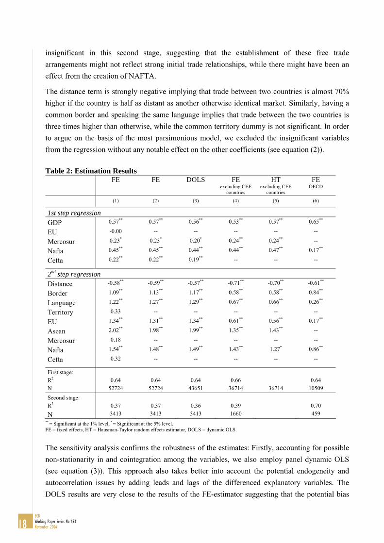
insignificant in this second stage, suggesting that the establishment of these free trade arrangements might not reflect strong initial trade relationships, while there might have been an effect from the creation of NAFTA.

The distance term is strongly negative implying that trade between two countries is almost 70% higher if the country is half as distant as another otherwise identical market. Similarly, having a common border and speaking the same language implies that trade between the two countries is three times higher than otherwise, while the common territory dummy is not significant. In order to argue on the basis of the most parsimonious model, we excluded the insignificant variables from the regression without any notable effect on the other coefficients (see equation (2)).

Table 2: Estimation Results FE FE DOLS FE

excluding CEE countries

HT excluding CEE

countries

FE OECD

(1) (2) (3) (4) (5) (6)

1st step regression

GDP 0.57** 0.57** 0.56** 0.53** 0.57** 0.65**

EU -0.00 -- -- -- -- --

Mercosur 0.23* 0.23* 0.20* 0.24** 0.24** --

Nafta 0.45** 0.45** 0.44** 0.44** 0.47** 0.17**

Cefta 0.22** 0.22** 0.19** -- -- -- 2nd step regression

Distance -0.58** -0.59** -0.57** -0.71** -0.70** -0.61**

Border 1.09** 1.13** 1.17** 0.58** 0.58** 0.84**

Language 1.22** 1.27** 1.29** 0.67** 0.66** 0.26**

Territory 0.33 -- -- -- -- --

EU 1.34** 1.31** 1.34** 0.61** 0.56** 0.17**

Asean 2.02** 1.98** 1.99** 1.35** 1.43** --

Mercosur 0.18 -- -- -- -- --

Nafta 1.54** 1.48** 1.49** 1.43** 1.27* 0.86**

Cefta 0.32 -- -- -- -- -- First stage: R2

0.64

0.64

0.64

0.66

0.64

N 52724 52724 43651 36714 36714 10509 Second stage: R2

0.37

0.37

0.36

0.39

0.70

N 3413 3413 3413 1660 459 ** = Significant at the 1% level, * = Significant at the 5% level. FE = fixed effects, HT = Hausman-Taylor random effects estimator, DOLS = dynamic OLS.

The sensitivity analysis confirms the robustness of the estimates: Firstly, accounting for possible non-stationarity in and cointegration among the variables, we also employ panel dynamic OLS (see equation (3)). This approach also takes better into account the potential endogeneity and autocorrelation issues by adding leads and lags of the differenced explanatory variables. The DOLS results are very close to the results of the FE-estimator suggesting that the potential bias


from the FE-specification should be small. As a second robustness check, two alternative samples have been estimated. Equation (4) excludes the transition countries as the inclusion of countries may have undesirable effects on the estimates (see Bussière, Fidrmuc and Schnatz 2005). With the exception of the border and the language dummies – both of which are dropping notably – the results are very stable. The distance term is only slightly higher and the dummies included for free trade arrangements are relatively close to the estimates shown before. For this sample, the Hausman-Taylor estimator shows once more that the specification is very robust to using different econometric methods (see equation (5)). Thirdly, as another robustness check, we restrained our sample to the OECD countries.22 Although the number of observations drops by roughly 80%, the results are broadly robust (see equation (6)). The variable for economic size and distance are still highly significant and the coefficients are rather close to those estimated in the full model. The coefficients of the time-invariant variables for having a common border and speaking the same language as well as the dummy variables for participation in a FTA are smaller.23

4. Extracting information from the predicted values The results of the gravity model can be interpreted in two different and complementary ways. We start with Section 4.1 with the predicted values obtained from the first stage of the fixed-effect regression, looking at selected country-pair examples, while section 4.2 delves into the interpretation of the second stage results.

4.1. Results from the first-stage regression

To facilitate the interpretation of the results, we examine the ratio of the actual (i.e. observed) divided by predicted trade flows, in percent (see Chart appendix).24 For instance, the first chart (France/Germany) shows that trade flows between the two countries rose in the early 1980s by 20% above the value predicted by the model, before quickly returning to the region implied by our right-hand side variables. A quick glance at most of the other charts for developed countries suggests that the model successfully captures the evolution of trade flows over time: the actual values are often in the same ballpark as the observed values, and the ratios tend to rapidly converge back to 100% when they depart from it.

Partly, this result depends to a large extent on the fixed effects, which ensure that the residuals are equal to zero on average (equivalently, they ensure that the ratios are equal to 100 on average for each country pair). However, even controlling for the between information (i.e. the fixed 22 In this specification, several variables used in the full model drop out as there are no relevant observations (e.g.

Mercosur, Cefta or common territory). 23 Bootstrapping increases in some cases the standard errors, but the conclusions on the significance of the variables

at standard levels is unaffected (this was done with 1000 replications). 24 The predicted values correspond to the projected values of the first stage fixed effect estimation of column 1,

Table 1. To compute the ratios, both actual and predicted trade values have been “unlogged”.

19ECB


effects), the model satisfactorily explains the within dimension of the panel. The fact that the ratio remains around 100% and does not show a clear trend over time also means that the time-varying right-hand side variables of the regression successfully capture the evolution of bilateral trade flows across countries. This is clearly the case for countries pairs like France/Germany, Germany/Italy, USA/France, Germany/USA, Germany/UK or France/UK. Among the developed economies, the country-pair France/Italy is an important exception: in the late 1980s/early 1990s, as well as in the early 2000s, the observed trade flows between these two countries have increased by a smaller amount than predicted. A closer look at the data shows that the trade flows between France and Italy slowed down in both directions in these two periods. These two periods also correspond to two waves of integration of EU countries in Europe.

The Canada-US country pair provides an interesting example of the sometimes powerful effect of FTAs on predicted trade flows: the completion of the 1988 agreement increased the predicted value of trade (the denominator), resulting in a fall of the ratio from 120 to 80. This result highlights a potential pitfall of capturing the effect of FTAs using coefficients which are estimated on the basis of shift dummies across many country pairs: often, the effect of FTAs itself is heterogeneous across countries and starts before the official completion of the treaties and takes time, sometimes several years, to reach its full impact. In the case of NAFTA, one might infer that the effect was larger on the Mexican/USA country pair than on the Canada/USA country pair.

Turning to trade flows between developed countries and China, in most cases, the ratios of actual to predicted trade flows remain close to 100%. This suggests that the dynamics of observed trade flows with China are successfully captured by our right-hand side variables. In other words, the growth of China’s trade flows with most developed countries seems roughly in line with GDP growth rates and the other policy variables. This situation contrasts with trade flows between euro area countries and other transition economies such as the new EU Member States, for which the actual to predicted ratios are strongly upward trending (see for instance trade between Germany and the Slovak Republic in the Chart Appendix). Bussière, Fidrmuc and Schnatz (2005) suggested that this increase can be interpreted as a convergence towards equilibrium: in the beginning of the transition period, the Eastern European countries were trading far below potential (i.e. below the value corresponding to the fundamentals), and they later on progressively caught up with fundamentals, implying that actual trade rose faster than predicted trade in the 1990s.

For China, the ratios tend to be fluctuating around 100 with the developed Asian countries (Japan, Hong Kong and Singapore). This highlights that the right-hand side variables are very successful in capturing the evolution of trade flows between China and these countries over time. By contrast, the ratios are strongly upward trending with the other developed countries in Asia (like Indonesia, Malaysia, South Korea, etc.), with an accelerating pattern in recent years. A


possible interpretation of these results can be related to the ongoing relocation of production of firms based in other emerging markets in Asia into China.

Finally, a back-of-the-envelope calculation shows that the model can account for the large increase of China’s trade flows in recent years and, thus, captures longer term trends in international trade. Over the period 1994-2002, China’s trade rose by nearly 140% (in constant dollar terms), while China’s real GDP roughly doubled and the GDP of the rest of the world rose by slightly over 40%. Using the coefficients reported in Table 2 together with the time dummies reflecting more general globalisation trends, the model predicts that China’s trade flows should have risen by a bit more than 150%, which is just slightly higher than the 140% actually recorded over this period. This example suggests that over longer periods, the model satisfactorily captures the evolution of trade flows. Over short horizons, however, the model’s predictions are less accurate. Indeed, in 2003, real GDP increased by around 10% for China and by less than 5% for the rest of the world which, together with the information provided by the time dummies, implies a rise in China’s trade flows by at most 9%. However, in 2003, China’s trade flows rose by more than 30%. On the one hand, this confirms that gravity models are not well suited for forecasting trade flows at an annual frequency; on the other hand, it may also suggest that the very strong growth rate in Chinese trade recorded after 2003 may be exceptional. The detailed account of the results provided in the Chart Appendix suggests that it is especially trade between China and the other Asian countries that rose fast in recent years (and in particular in 2003).

4.2 Results from the second stage regression: extracting information from country-heterogeneity

Overall trade intensity of countries

While Cheng and Wall (2005) call the fixed effects a “result of ignorance” for the estimation, they include valuable information for analysing the degree of integration of these countries into the world economy. In more detail, the residuals of the second stage regression can be interpreted as measures of trade integration after controlling for the relevant fundamentals of the gravity equation. As regards the relevant fundamentals, we corrected the residuals for the estimated impact of FTAs shown in the second step of the regression for two reasons. Firstly, the high absolute value of the coefficients associated with FTAs is likely to mainly reflect a high degree of integration of countries establishing a FTA rather than the effect of the FTA itself, which should be reflected in a measure of trade integration. Secondly, FTAs are – in contrast to state variables such as distance or economic size – the main policy-related variables included in the estimation. At the same time, it is important to include these variables into the regression in order to avoid an estimation bias owing to omitted variables. Accordingly, the adjusted residuals denoted by

*ˆ ˆij ij k kk FTA

Zµ µ γ=

= − ∑ (3)

21ECB


and aggregated those for a country h into a new empirical indicator of “trade integration”, tih: 1 1

* *

1 1

1 ˆ ˆ2( 1)

N N

h ih hji j

tiN

µ µ− −

= =

⎛ ⎞= +⎜ ⎟− ⎝ ⎠

∑ ∑ (4)

For a given country h, a high tih – reflecting strongly positive average residuals of a country – signifies that this country has on average strong trade links with the rest of the world, while strongly negative average residuals indicate relatively low trade intensity. Chart 1 ranks the indicator of trade intensity for all countries in ascending order implying that the indicator of trade integration declines from the left to the right (based on equation (2) above).

Chart 1 provides four key insights. Firstly, the variance of the indicators reveals a considerable degree of heterogeneity across countries. Secondly, most industrialised countries – particularly the USA, Japan and Germany – tend to display above-average trade integration.25 Thirdly, the South-East Asian countries show a high trade indicator and, thus, little overall trade resistance.26 The fact that the Asian countries are found on the left-hand side of the spectrum is relatively intuitive as these countries are commonly known to be very open to external trade and have very strong trade connections with the rest of the world. In this context, it is noteworthy how well China is already integrated into the world economy. China is even among the Asian countries more integrated into the global economy than Malaysia, Thailand and Indonesia, albeit less so than Japan and the tiger economies of Hong Kong, South Korea and Singapore. Fourthly, at the other end of the spectrum are many transition economies in Central and Eastern Europe which are by far less integrated into the world, as analysed in detail in Bussière, Fidrmuc and Schnatz (2005).

The heterogeneity of trade integration across countries could be an interesting subject for future research and we just mention a few possible explanations, with a special focus on China. First, the structural composition of trade varies a lot across countries, which is also likely to affect the value added implied in trade flows. For countries such as the Netherlands transit trade accounts for a substantial part of trade flows and “artificially” increases the value of exports and imports. For China, in particular, process trade is estimated to account for around 40% of total exports27, which may partly explain why trade flows are so high with China. Second, foreign direct investment is likely to play an important role. It is estimated, for instance, that more than half of Chinese exports are produced by foreign funded firms.28 This is related to the fact that China, owing to its low production costs, is increasingly used as an export platform by foreign companies, especially by other Asian countries such as Japan. However, Eastern European countries also received significant foreign direct investment in recent years, such that further

25 Exceptions are Luxembourg and Greece which appear to face a somewhat higher level of overall trade resistance

which in the case of Luxembourg may be due to the specific structure of the economy. 26 This may partly reflect strong intra-regional integration and a relatively low domestic value-added in their

exports. 27 Source: CEIC; see http://www.ceicdata.com. 28 See also CEIC; http://www.ceicdata.com.


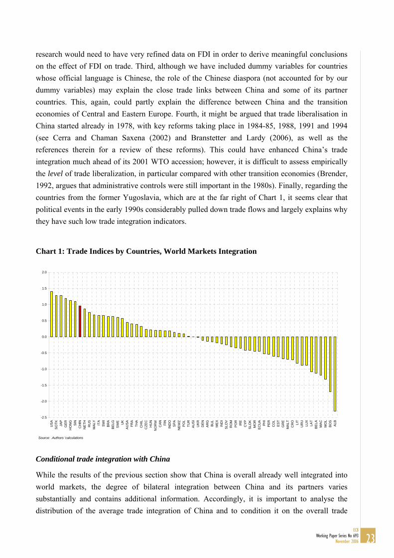
research would need to have very refined data on FDI in order to derive meaningful conclusions on the effect of FDI on trade. Third, although we have included dummy variables for countries whose official language is Chinese, the role of the Chinese diaspora (not accounted for by our dummy variables) may explain the close trade links between China and some of its partner countries. This, again, could partly explain the difference between China and the transition economies of Central and Eastern Europe. Fourth, it might be argued that trade liberalisation in China started already in 1978, with key reforms taking place in 1984-85, 1988, 1991 and 1994 (see Cerra and Chaman Saxena (2002) and Branstetter and Lardy (2006), as well as the references therein for a review of these reforms). This could have enhanced China’s trade integration much ahead of its 2001 WTO accession; however, it is difficult to assess empirically the level of trade liberalization, in particular compared with other transition economies (Brender, 1992, argues that administrative controls were still important in the 1980s). Finally, regarding the countries from the former Yugoslavia, which are at the far right of Chart 1, it seems clear that political events in the early 1990s considerably pulled down trade flows and largely explains why they have such low trade integration indicators.

Chart 1: Trade Indices by Countries, World Markets Integration

-2.5

-2.0

-1.5

-1.0

-0.5

0.0

0.5

1.0

1.5

2.0

US

ASO

TK JAP

GE

RH

ON

GS

INC

HIN

NE

THR

US

MA

LY ITA

SW

IB

RA

BE

LGS

WE

UK

AU

SA

FRA

THA

CH

ILC

ZEC

HU

NN

OR

WC

AN

FIN

IND

OS

PA

NE

WZ

PO

LTU

RA

US

IU

KR

DE

NA

RG

BU

LM

EX

IND

IS

LOV

RO

MP

OR

IRE

CY

PS

LOK

MO

RE

CU

AP

HI

PE

RC

OL

ES

TG

RE

MA

LTC

RO

LIT

UR

ULU

XLA

TB

ELA

MA

CM

OL

BO

SA

LB

Source: .Authors 'calculations

Conditional trade integration with China

While the results of the previous section show that China is overall already well integrated into world markets, the degree of bilateral integration between China and its partners varies substantially and contains additional information. Accordingly, it is important to analyse the distribution of the average trade integration of China and to condition it on the overall trade

23ECB


integration of each trading partner (this is done in Chart 2). For example, the United States is in Chart 1 the country most integrated into world markets (trade integration index amounting to about 1.4). At the same time, the United States is even more integrated with China, having a trade integration index of about 3.2 (this represents the residual of the second stage regression corresponding to the country-pair China/USA). This implies that after controlling for the fundamentals of the gravity model the United States trades much more with China than with the average trading partner. The integration of the United States with China conditional on the overall integration of the United States amounts to about 1.8 (subtracting 1.4 from 3.2). In order to illustrate the concept it is also worthwhile to consider the case of Albania which is the least globally-integrated country in the sample (ti=-2.3). China’s trade integration with Albania is also very limited (ti=-1.4) but given Albania’s low global trade integration standards, these two countries are in fact fairly well integrated. This conditional trade integration index with China has been computed for each country and ascendingly ordered in Chart 2.

Chart 2: Conditional Trade Indices by Countries, Integration with China as Compared with Overall Integration

-2.5

-2.0

-1.5

-1.0

-0.5

0.0

0.5

1.0

1.5

2.0

2.5

CA

NPE

RAU

SA

IND

OU

RU

MAL

YU

SA

PH

IA

RG

GE

RN

EW

ZTH

AFR

AN

ETH

BE

LGSP

AU

KR

JAP

FIN

UK

ITA

DE

NSO

TKM

EX

MO

RG

RE

IRE

MA

LTBR

ASW

ER

OM

ALB

AU

SI

HU

NP

OL

HO

NG

BE

LALU

XE

CU

AS

INN

OR

WS

WI

TUR

CZE

CC

YP

ES

TR

US

CO

LP

OR

SLO

KC

RO

BU

LS

LOV

IND

ILI

TLA

TM

AC

MO

LB

OS

Source: Authors' calculations

Chart 2 suggests that China is very well integrated with Canada, Australia, the United States and several Latin American countries (Peru, Uruguay and Argentina). These countries are more integrated with China than many emerging economies in Asia and Japan. It is interesting to note that Singapore and Hong Kong can only be found towards the right hand side of the spectrum. We know of course from Table 1 that Hong Kong is particularly well integrated with China based


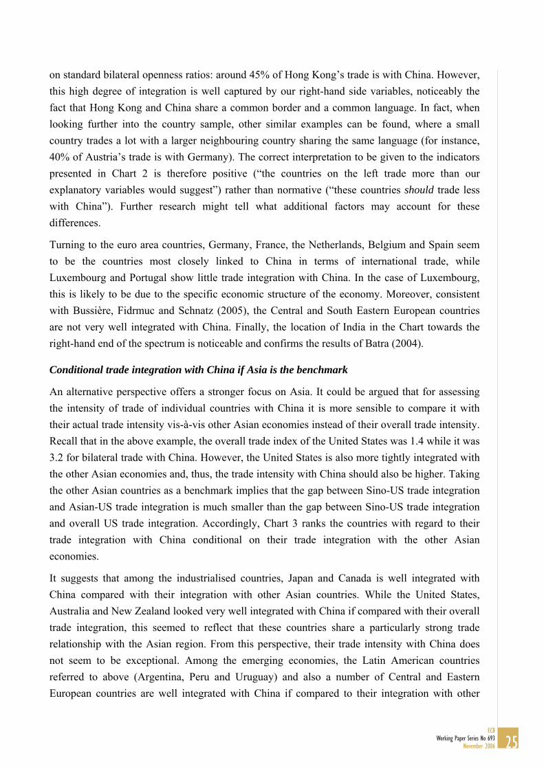
on standard bilateral openness ratios: around 45% of Hong Kong’s trade is with China. However, this high degree of integration is well captured by our right-hand side variables, noticeably the fact that Hong Kong and China share a common border and a common language. In fact, when looking further into the country sample, other similar examples can be found, where a small country trades a lot with a larger neighbouring country sharing the same language (for instance, 40% of Austria’s trade is with Germany). The correct interpretation to be given to the indicators presented in Chart 2 is therefore positive (“the countries on the left trade more than our explanatory variables would suggest”) rather than normative (“these countries should trade less with China”). Further research might tell what additional factors may account for these differences.

Turning to the euro area countries, Germany, France, the Netherlands, Belgium and Spain seem to be the countries most closely linked to China in terms of international trade, while Luxembourg and Portugal show little trade integration with China. In the case of Luxembourg, this is likely to be due to the specific economic structure of the economy. Moreover, consistent with Bussière, Fidrmuc and Schnatz (2005), the Central and South Eastern European countries are not very well integrated with China. Finally, the location of India in the Chart towards the right-hand end of the spectrum is noticeable and confirms the results of Batra (2004).

Conditional trade integration with China if Asia is the benchmark

An alternative perspective offers a stronger focus on Asia. It could be argued that for assessing the intensity of trade of individual countries with China it is more sensible to compare it with their actual trade intensity vis-à-vis other Asian economies instead of their overall trade intensity. Recall that in the above example, the overall trade index of the United States was 1.4 while it was 3.2 for bilateral trade with China. However, the United States is also more tightly integrated with the other Asian economies and, thus, the trade intensity with China should also be higher. Taking the other Asian countries as a benchmark implies that the gap between Sino-US trade integration and Asian-US trade integration is much smaller than the gap between Sino-US trade integration and overall US trade integration. Accordingly, Chart 3 ranks the countries with regard to their trade integration with China conditional on their trade integration with the other Asian economies.

It suggests that among the industrialised countries, Japan and Canada is well integrated with China compared with their integration with other Asian countries. While the United States, Australia and New Zealand looked very well integrated with China if compared with their overall trade integration, this seemed to reflect that these countries share a particularly strong trade relationship with the Asian region. From this perspective, their trade intensity with China does not seem to be exceptional. Among the emerging economies, the Latin American countries referred to above (Argentina, Peru and Uruguay) and also a number of Central and Eastern European countries are well integrated with China if compared to their integration with other

25ECB


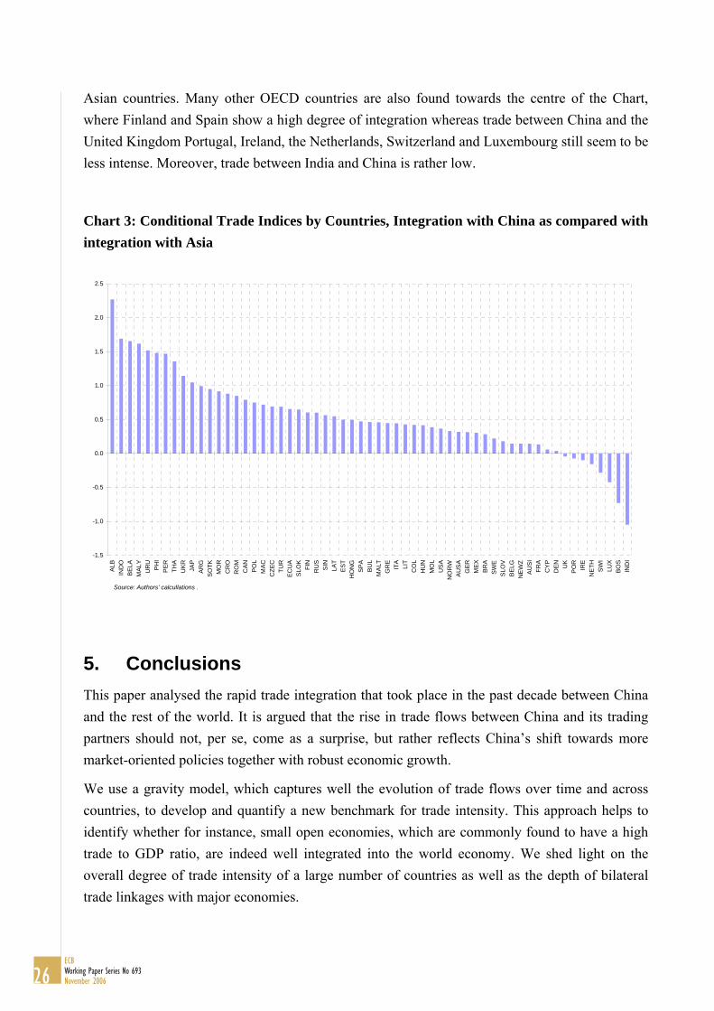
Asian countries. Many other OECD countries are also found towards the centre of the Chart, where Finland and Spain show a high degree of integration whereas trade between China and the United Kingdom Portugal, Ireland, the Netherlands, Switzerland and Luxembourg still seem to be less intense. Moreover, trade between India and China is rather low.

Chart 3: Conditional Trade Indices by Countries, Integration with China as compared with integration with Asia

-1.5

-1.0

-0.5

0.0

0.5

1.0

1.5

2.0

2.5

ALB

IND

OB

ELA

MA

LYU

RU

PH

IP

ER THA

UKR JA

PA

RG

SO

TKM

OR

CR

OR

OM

CAN PO

LM

AC

CZE

CTU

RE

CU

AS

LOK

FIN

RU

SS

INLA

TE

STH

ON

GSP

AB

UL

MA

LTG

RE

ITA

LIT

CO

LH

UN

MO

LU

SA

NO

RW

AU

SA

GER

ME

XB

RA

SWE

SLO

VB

ELG

NE

WZ

AU

SI

FRA

CY

PD

EN UK

PO

RIR

EN

ETH SW

ILU

XBO

SIN

DI

Source: Authors' calcullations .

5. Conclusions This paper analysed the rapid trade integration that took place in the past decade between China and the rest of the world. It is argued that the rise in trade flows between China and its trading partners should not, per se, come as a surprise, but rather reflects China’s shift towards more market-oriented policies together with robust economic growth.

We use a gravity model, which captures well the evolution of trade flows over time and across countries, to develop and quantify a new benchmark for trade intensity. This approach helps to identify whether for instance, small open economies, which are commonly found to have a high trade to GDP ratio, are indeed well integrated into the world economy. We shed light on the overall degree of trade intensity of a large number of countries as well as the depth of bilateral trade linkages with major economies.


The comparison of actual and predicted trade flows shows that for most country-pairs, the model successfully captures the evolution of bilateral trade over time. Overall, the rapid integration of China in world markets is well reflected by the fundamentals in the case of many developed countries in Western Europe and North America. These results tend to put in perspective the strong growth in bilateral trade flows between China and its partner countries.29

Moreover, our new measure of trade intensity suggests that China is overall already very well integrated in world markets. Comparing the trade intensity of China across countries and using the overall trade intensity of these countries is taken as a benchmark suggests that China is well integrated with the United States, Canada, Australia and several Latin American countries. Among the euro area countries, Germany, France, the Netherlands, Belgium and Spain seem to be the country most closely linked to China in terms of international trade, while Luxembourg and Portugal show little trade integration with China. Using instead the partner countries’ trade intensity vis-à-vis other Asian countries as a benchmark confirms, on the one hand, the close ties between China and Canada as well as the Latin American countries and the low trade intensity between India and China. Notably, however, for the United States and Australia the trade ties with China do not seem to be extraordinarily high if compared with their trade intensity with other countries in the Asian region.

29 However, it does not mean of course that the trade integration of China is neutral to the welfare of the other

countries. For instance, one key issue, not tackled in this paper, is the fact that China’s trade integration is not even across sectors (see e.g. Rodrik (2006)), which may imply a necessary reallocation of resources across sectors. Holzmann, Thimann and Pelz (1993) provided an early analysis of the impact on OECD economies of the trade integration of transition countries and of the possible policy reforms. See Mandelson (2006) for a recent policy discussion.

27ECB


References

Abraham, F. and J. Van Hove (2005). “The rise of China: Prospects of regional trade policy”. Weltwirtschaftliches Archiv/Review of World Economics, 141, 3, 486-509.

Anderson, J. E. (1979). “A theoretical foundation for the gravity equation”. American Economic Review 69, 1, 106-116.

Anderson, J. E. and E. van Wincoop (2003). “Gravity with gravitas: a solution to the border puzzle”. American Economic Review, 93, 1, 170-192.

Anderton, R., F. di Mauro and F. Moneta (2004). “Understanding the Impact of the External Dimension of the Euro Area: Trade, Capital flows and Other International Macroeconomic Linkages”, ECB Occasional Paper, 12.

Baldwin, R. E. (1994). “Towards an integrated Europe”. CEPR, London.

Baldwin, R. E. and D. Taglioni (2006). “Gravity for dummies and dummies for gravity equations” NBER Working Paper, 12516.

Batra, A. (2004). “India’s global trade potential: the gravity model approach”. ICRIER Working Paper, 151.

Bénassy-Quéré, A. and A. Lahrèche-Révil (2003). “Trade linkages and exchange rates in Asia: the role of China”. CEPII Working Paper, 2003-21.

Blattner, T. S. (2005). “What drives foreign direct investment in Southeast Asia? A dynamic panel approach”. Mimeo, European Central Bank.

Boorstin, D. J. (1983). “The Discoverers”, Random House Publisher.

Branstetter, L. and N. Lardy (2006). “China’s embrace of globalisation”. NBER Working Paper, 12373.

Brender, A. (1992). “China’s Foreign Trade Behavior in the 1980s: an Empirical Analysis”, IMF Working Paper, WP/92/5.

Bussière, M., J. Fidrmuc and B. Schnatz (2005). “Trade integration of Central and Eastern European countries: Lessons from a gravity model”. European Central Bank Working Paper, 545.

Cerra, V. and S. Chaman Saxena (2002). “An Empirical analysis of China’s Export Behaviour”, IMF Working Paper, WP/02/200.

Chang, G. and Q. Shao (2004). “How much is the Chinese currency undervalued? A quantitative estimation”. China Economic Review, 15, 2004, 366– 371.

Cheng, I-H. and H. J. Wall (2005). “Controlling for heterogeneity in gravity models of trade and integration”. Federal Reserve Bank of St. Louis Review, 87, 1, 49-63.

Coudert, V. and C. Couharde (2005). “Real Equilibrium Exchange Rate in China”. CEPII Working Paper 2005-1.

Deardorff, A.V. (1995). “Determinants of bilateral trade: does gravity work in a neoclassical world?”. NBER Working Paper, 5377.


Egger, P. (2003). “An econometric view on the estimation of gravity models and the calculation of trade potentials”. The World Economy, 25, 2, 297-312.

Egger, P. (2004). “Estimating regional trading bloc effects with panel data”. Weltwirtschaftliches Archiv, 140, 1, 151-166.

Egger, P. and M. Pfaffermayr (2003). “The proper panel econometric specification of the gravity equation: A three-way model with bilateral interaction effects”. Empirical Economics, 28, 571-580.

Egger, P. and M. Pfaffermayr (2004). “Distance, trade and FDI: a Hausman-Taylor SUR approach”. Journal of Applied Econometrics, 19, 2, 227-246.

Eichengreen, B, Y. Rhee and H. Tong (2004). “The impact of China on the exports of other Asian countries”. NBER Working Paper, 10768.

Faruqee, H. (2004). “Measuring the trade effects of EMU”. IMF Working Paper, 04/154.

Fidrmuc, J. (2006). “Gravity Models and Cross-Sectional Correlation in Integrated Panels”. mimeo, University of Munich, Department of Economics; CESifo Institute Munich; and Comenius University Bratislava, Slovakia.

Fidrmuc, J. and J. Fidrmuc (2003). “Disintegration and trade”. Review of International Economics, 11, 5, 811-829.

Filippini, C., V. Molini and D. Pozzoli (2005). “The determinants of East Asia trade flows: A gravity equation approach”. Mimeo, Bocconi University.

Frankel, J. (1997). “Regional trading blocs in the world economic system”, Institute for International Economics, Washington, D. C.

Frankel, J. (2005). “On the renminbi”. CESifo Forum 3/2005, 16-21.

Graham, C., J. Helliwell, T. Kano, J. Murray, L. Schembri (2004). “The Euro and trade: is there a positive effect?”. Mimeo, Bank of Canada, presented at the Annual Meetings of the Canadian Economics Association.

Hausman, J. A. and W. E. Taylor (1981). “Panel data and unobservable individual effects”. Econometrica, 49, 6, 1377-1398.

Holzmann, R., C. Thimann and A. Petz (1993). “Pressure to Adjust: Consequences for the OECD Countries from Reforms in Eastern Europe”, University of Munich.

Kaminski, B., Wang, Z. K. and L. A. Winters (1996). “Trade performance, export reorientation in the transition”. Economic Policy, October 1996, 421-442.

Kao, C. and M.-H Chiang. (2000). “On the estimation and inference of cointegrated regression in panel data”. Advances in Econometrics 15, 179-222.

Koukhartchouk O. and M. Maurel (2003). “Russia's Accession to the WTO: The Potential for Trade Increase”, Journal of Comparative Economics, 32, 4, 599-825.

Lee, J.-W. and I. Park (2005). “Free trade areas in East Asia: Discriminatory or non-Discriminatory ?”. The World Economy, 28, 1, 1-145.

Linder, S. (1961). “An essay on trade and transformation”. Uppsala: Almqvist and Wiksells eds.

29ECB


Linnemann, H. (1966). “An econometric study of international trade flows”. Amsterdam: North Holland.

McCallum, J. (1995). “National Borders Matter: Canada-U.S. Regional Trade Patterns”. American Economic Review, 85, 615-23.

Mandelson, P. (2006) “Europe’s response to globalisation: where does EU trade policy go from here? ”. Speech, Wolfsberg, Switzerland, 4 May 2006. http://ec.europa.eu/commission_barroso/mandelson/speeches_articles/sppm096_en.htm.

Markusen, J.R. and A.J. Venables (1998). “Multinational firms and the new trade theory”. Journal of International Economics, 46, 2, 183-203.

Mátyás, L. (1997). “Proper econometric specification of the gravity model”. The World Economy, 20, 3, 363-368.

Mátyás, L. (1998). “The gravity model: Some econometric considerations”. The World Economy, 21, 3, 397-401.

McKibbin, W. and W. T. Woo (2002). “The consequences of China’s WTO Accession on its Neighbours”, http://www.sensiblepolicy.com/.

Micco, A., E. Stein and G. Ordoñez (2003). “The Currency Union Effect on Trade: Early Evidence from EMU”. Economic Policy, 315-356.

Prasad, E. (2004). “China’s Growth and Integration into the World Economy”. IMF Occasional Paper, OP/232/2004.

Rodrik, D. (2006). “What’s so special about China’s exports?”. NBER Working Paper, 11947.

Rose, A. K. (2000). “One Money, One Market: Estimating the Effect of Common Currencies on Trade”. Economic Policy: A European Forum, 15, 7-45.

Rumbaugh, T. and N. Blancher (2004). “China: Inernational Trade and WTO Accession”. IMF Working Paper, WP/04/36.

Schindler, J. and D. Beckett (2005). “Adjusting Chinese Bilateral Trade Data: How Big is China’s Trade Surplus?”. Board of Governors of the Federal Reserve System, International Finance Discussion Papers, 831.

Schott, P. K. (2006). “The relative sophistication of Chinese exports”. NBER Working Paper 12173.

Serlenga, L. and Y. Shin (2004). “Gravity models of the intra-EU trade: Application of the Hausman-Taylor estimation in heterogeneous panels with common time-specific factors”. Mimeo, University of Edinburgh.

Yang, Y. (2003). “China’s Integration into the World Economy: Implications for Developing countries”. IMF Working Paper, WP/03/245.


Data Sources Countries included: Albania, Algeria, Argentina, Australia, Austria, Belarus, Belgium, Bosnia, Brazil, Bulgaria, Canada, Chile, China, Colombia, Croatia, Cyprus, Czech Republic, Denmark, Ecuador, Estonia, Finland, France, Germany, Greece, Hong Kong, Hungary, India, Indonesia, Ireland, Italy, Japan, Latvia, Lithuania, Luxembourg, Macedonia, Malaysia, Malta, Mexico, Moldova, Morocco, Netherlands, New Zealand, Norway, Peru, Philippines, Poland, Portugal, Romania, Russia, Singapore, Slovak Republic, Slovenia, South Korea, Spain, Sweden, Switzerland, Thailand, Turkey, United Kingdom, Ukraine, Uruguay, USA.

Trade data: IMF DOTS.

GDP: IFS line 99b. For Ecuador data from WDI. Data for Greece up to 1994 from WDI. Date for Turkey up to 1985 from WDI. If there was a large discrepancy between World Bank and IMF data, observations have been dropped. This includes Argentina (1980-84), Bulgaria (1985-92), China (1980-1993), Estonia, Latvia, Lithuania (each 1993-95), Moldova (1995), Russia (1993-94), Ukraine (1993-95), for Albania, Bosnia and Herzegovina, Moldova and Macedonia data from EBRD.

Distance: Great circle distances based on MS Encarta World Atlas software.

Exchange rate: IFS line rf. Exchange rates for individual euro area countries were chain-lined with the euro exchange rate upon EMU entry.

Consumer prices: IFS line 64. For Belarus, China, Russia and the Ukraine, inflation rates (IFS line 64.xx) were transformed into price indices.

Industrial producer price: IFS line 63a for the United States.

Real exchange rate: Product of the US dollar exchange rate and the ratio of domestic and foreign consumer prices.

Exchange rate volatility: Standard deviation of the month-on-month log changes in the bilateral nominal exchange rate within a year.

Common border: A matrix is available upon request.

Common language: Based on a matrix including the following languages: English (Australia, Canada, India, Ireland, Hong Kong, Malta, New Zealand, Philippines, Singapore, United Kingdom and the USA), Spanish (Argentina, Chile, Colombia, Ecuador, Mexico, Peru, Spain, Uruguay, Venezuela), French (Algeria, Belgium, Canada, France, Luxembourg, Morocco, Switzerland), German (Austria, Germany, Luxembourg, Switzerland), Chinese (China, Hong Kong, Singapore), Russian (Belarus, Estonia, Latvia, Lithuania, Moldova, Russia, Ukraine), Dutch (Belgium, Netherlands), Greek (Greece, Cyprus), Arabic (Algeria, Morocco), Serbo-Croatian (Bosnia, Croatia, Slovenia), Portuguese (Brazil, Portugal), Swedish (Sweden, Finland), Albanian (Albania, Macedonia), Malay (Malaysia, Singapore).

Free-trade agreement: ASEAN Association of South East Asian Nations (1967): Brunei (1984), Cambodia (1999), Indonesia, Laos (1997), Malaysia, Myanmar (1997), Philippines, Singapore, Thailand, Vietnam (1995), CEFTA Central European Free Trade Agreement (1994): Bulgaria (1999), Czech Republic, Hungary, Poland, Romania, Slovak Republic, Slovenia (1997), European Union (EU15):Austria (1995), Belgium, Denmark, Finland (1995), France, Germany, Greece (1981), Ireland, Italy, Luxembourg, Netherlands, Portugal (1986), Spain (1986), Sweden (1995), United Kingdom, European Union (EU15) and Customs Unions: EU15, Cyprus, Malta, Turkey (1996); MERCOSUR Southern Common Market (1993): Argentina Brazil Paraguay Uruguay, NAFTA North American Free Trade Agreement: Canada (1988), Mexico (1993), United States (1988).

Common territory includes countries which constituted in the past 20 years at some point a common country. They include a) former Czechoslovakia (the Czech Republic and the Slovak Republic), b) countries of the former Soviet Union (Belarus, Estonia, Latvia, Lithuania, Moldova, Russia and the Ukraine, and c) countries of former Yugoslavia (Bosnia, Croatia, Macedonia, Slovenia).

31ECB


CHART APPENDIX Acronyms: Rest of Asia (ROA), New EU Member States (NMS); see country list in Table 3.

Chart A1: Extra-euro area trade shares. (percent of total extra-euro area trade)

0

2

4

6

8

10

12

14

16

18

20

1980

1982

1984

1986

1988

1990

1992

1994

1996

1998

2000

2002

2004

Source: IMF DOTS.Note: Last observation refers to 2005.

UK

USA

NMS

R. O. A.

China

Japan

Chart A2: Trade shares, Germany. (percent of total trade)

0

2

4

6

8

10

12

14

1980

1982

1984

1986

1988

1990

1992

1994

1996

1998

2000

2002

2004


France

NMS

USA

UK

Italy

China

Chart A3: Trade shares, France. (percent of total trade)

0

2

4

6

8

10

12

14

16

18

20

1980

1982

1984

1986

1988

1990

1992

1994

1996

1998

2000

2002

2004


Germany

Italy

UK

USA

NMS

China

Chart A4: Trade shares, Italy. (percent of total trade)

0

5

10

15

20

25

1980

1982

1984

1986

1988

1990

1992

1994

1996

1998

2000

2002

2004


Germany

France

USA

UK

NMS

China

Chart A5: Trade shares, USA. (percent of total trade)

0

5

10

15

20

25

1980

1982

1984

1986

1988

1990

1992

1994

1996

1998

2000

2002

2004


Canada

EuroAreaMexico

China

R. O. A.

Japan

UK

Chart A6: Trade shares, UK. (percent of total trade)

0

2

4

6

8

10

12

14

16

1980

1982

1984

1986

1988

1990

1992

1994

1996

1998

2000

2002

2004


Germany

USA

France

R. O. A.

Italy

China

Japan


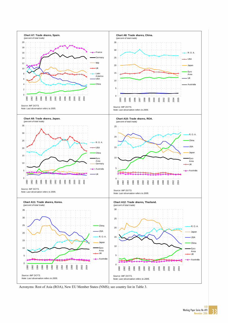
Chart A7: Trade shares, Spain. (percent of total trade)

0

2

4

6

8

10

12

14

16

18

20

1980

1982

1984

1986

1988

1990

1992

1994

1996

1998

2000

2002

2004


France

Germany

Italy

UK

LatinAmericaUSA

China

Chart A8: Trade shares, China. (percent of total trade)

0

5

10

15

20

25

30

35

1993

1994

1995

1996

1997

1998

1999

2000

2001

2002

2003

2004

2005


R. O. A.

USA

Japan

EuroArea

UK

Australia

Chart A9: Trade shares, Japan. (percent of total trade)

0

5

10

15

20

25

30

35

1980

1982

1984

1986

1988

1990

1992

1994

1996

1998

2000

2002

2004


R. O. A.

USA

China

EuroAreaGermany

Australia

UK

Chart A10: Trade shares, ROA. (percent of total trade)

0

5

10

15

20

25

1980

1982

1984

1986

1988

1990

1992

1994

1996

1998

2000

2002

2004


R. O. A.

China

USA

Japan

EuroAreaUK

Australia

Chart A11: Trade shares, Korea. (percent of total trade)

0

5

10

15

20

25

30

35

1980

1982

1984

1986

1988

1990

1992

1994

1996

1998

2000

2002

2004


China

USA

R. O. A.

Japan

EuroAreaUK

Australia

Chart A12: Trade shares, Thailand. (percent of total trade)

0

5

10

15

20

25

30

1980

1982

1984

1986

1988

1990

1992

1994

1996

1998

2000

2002

2004


R. O. A.

Japan

USA

China

EuroAreaUK

Australia

Acronyms: Rest of Asia (ROA), New EU Member States (NMS); see country list in Table 3.

33ECB


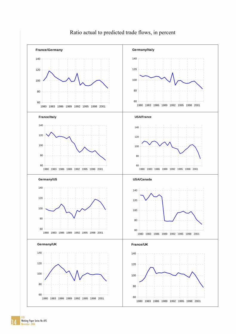
Ratio actual to predicted trade flows, in percent

France/Germany

60

80

100

120

140

1980 1983 1986 1989 1992 1995 1998 2001

Germany/Italy

60

80

100

120

140

1980 1983 1986 1989 1992 1995 1998 2001

France/Italy

60

80

100

120

140

1980 1983 1986 1989 1992 1995 1998 2001

USA/France

60

80

100

120

140

1980 1983 1986 1989 1992 1995 1998 2001 Germany/US

60

80

100

120

140

1980 1983 1986 1989 1992 1995 1998 2001

USA/Canada

60

80

100

120

140

1980 1983 1986 1989 1992 1995 1998 2001

Germany/UK

60

80

100

120

140

1980 1983 1986 1989 1992 1995 1998 2001

France/UK

60

80

100

120

140

1980 1983 1986 1989 1992 1995 1998 2001


China/USA

60

80

100

120

140

1994 1996 1998 2000 2002

China/France

60

80

100

120

140

1994 1996 1998 2000 2002

China/Germany

60

80

100

120

140

160

1994 1996 1998 2000 2002

China/UK

60

80

100

120

140

1994 1996 1998 2000 2002

China/Hong Kong

60

80

100

120

140

1994 1996 1998 2000 2002

China/Indonesia

60

80

100

120

140

1994 1996 1998 2000 2002

China/Japan

60

80

100

120

140

1994 1996 1998 2000 2002

China/Malaysia

60

80

100

120

140

160

180

200

220

1994 1996 1998 2000 2002

35ECB


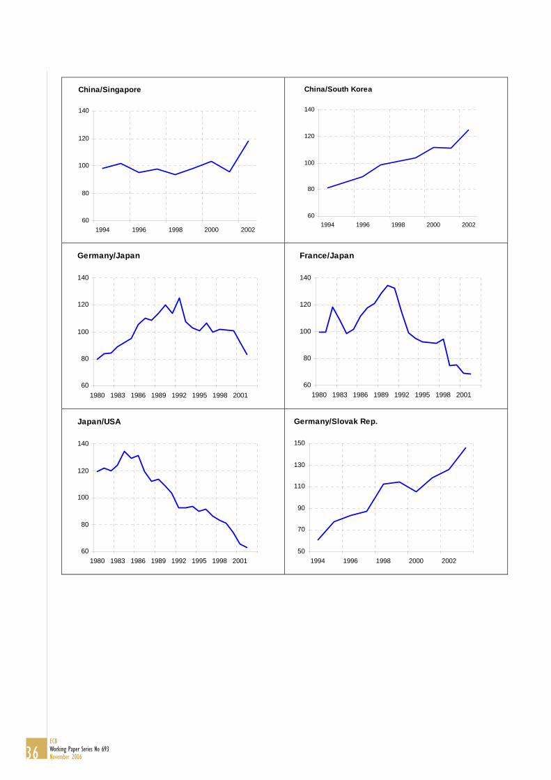
China/Singapore

60

80

100

120

140

1994 1996 1998 2000 2002

China/South Korea

60

80

100

120

140

1994 1996 1998 2000 2002

Germany/Japan

60

80

100

120

140

1980 1983 1986 1989 1992 1995 1998 2001

France/Japan

60

80

100

120

140

1980 1983 1986 1989 1992 1995 1998 2001

Japan/USA

60

80

100

120

140

1980 1983 1986 1989 1992 1995 1998 2001

Germany/Slovak Rep.

50

70

90

110

130

150

1994 1996 1998 2000 2002


TABLE APPENDIX Table 3: Selected Variables for the Countries Included in the Sample

1995 2005 p.c 1995 2005 p.c 1995 2005 p.c 1995 2005 p.c(A) (B) (C) (D) (E) (F) (G) (H) (I) (J) (K) (L) (M)

China 3.7 7.7 4.0 32.7 62.4 29.7 ND ND ND ND ND NDEuro AreaAustria 1.1 1.1 0.0 50.9 75.5 24.6 1.0 1.8 0.8 0.3 0.2 -0.1Belgium 2.8 2.7 -0.1 112.0 136.5 24.5 0.7 2.1 1.4 0.8 0.8 0.0Finland 0.7 0.6 0.0 52.4 62.6 10.2 1.4 3.6 2.1 0.3 0.4 0.2France 5.3 4.5 -0.8 33.7 43.5 9.8 1.4 2.7 1.3 1.6 1.5 -0.1Germany 9.2 8.2 -1.0 39.3 63.9 24.6 1.9 4.3 2.4 4.9 4.4 -0.4Greece 0.3 0.3 0.0 33.1 31.3 -1.8 1.0 3.1 2.1 0.1 0.1 0.1Ireland 0.7 1.0 0.3 114.5 86.1 -28.5 0.5 1.7 1.2 0.1 0.3 0.3Italy 3.9 3.5 -0.5 39.1 41.8 2.7 1.5 3.1 1.6 1.8 1.3 -0.5Luxembourg 0.2 0.2 0.0 104.2 95.2 -9.0 0.4 7.3 6.9 0.0 0.2 0.1Netherlands 3.5 3.4 -0.2 88.5 102.2 13.7 0.9 4.6 3.7 1.4 2.0 0.6Portugal 0.5 0.5 -0.1 50.4 53.0 2.6 0.4 0.9 0.5 0.1 0.1 0.0Spain 1.9 2.2 0.3 34.3 41.9 7.6 1.6 3.0 1.4 0.7 0.7 0.1Total 2/ 31.3 28.7 -2.6 44.8 58.2 13.4 1.6 3.8 2.2 12.0 12.1 0.1 extra-trade only 2/ 18.0 17.0 -1.0 21.7 29.7 8.0 3.0 6.6 3.6 ND ND NDOther developed countriesAustralia 1.1 1.1 0.0 29.8 32.0 2.2 4.7 12.7 8.0 1.5 1.9 0.4Canada 3.5 3.2 -0.4 61.1 61.4 0.3 1.6 4.6 3.0 1.5 1.3 -0.2Denmark 0.8 0.7 -0.1 53.0 61.6 8.7 1.1 2.9 1.7 0.2 0.3 0.1Japan 7.6 5.3 -2.2 13.8 22.8 9.0 7.4 17.0 9.6 20.4 13.0 -7.5New Zealand 0.3 0.2 0.0 43.1 43.0 -0.1 3.0 5.7 2.7 0.2 0.2 0.0Norway 0.7 0.8 0.0 51.6 54.2 2.6 1.1 2.0 0.9 0.2 0.2 0.0Sweden 1.3 1.2 -0.2 57.9 67.9 10.1 1.1 2.7 1.6 0.5 0.4 -0.1Switzerland 1.8 1.4 -0.4 52.1 69.6 17.5 1.0 2.0 1.0 0.5 0.4 -0.1UK 4.8 4.1 -0.8 44.4 40.2 -4.2 0.9 3.4 2.5 1.7 1.7 0.0USA 13.6 12.1 -1.5 17.9 20.6 2.7 4.4 11.4 7.0 14.5 14.9 0.4Other Emerging East Asian CountriesHong Kong 2.2 1.8 -0.4 254.1 330.1 76.0 34.8 45.0 10.2 15.9 9.6 -6.3Indonesia 0.8 0.8 -0.1 40.4 54.5 14.1 3.8 10.3 6.6 1.2 1.2 -0.1Malaysia 1.6 1.4 -0.2 161.3 190.5 29.2 2.4 10.4 8.1 1.2 2.2 1.0Philippines 0.5 0.5 0.1 58.0 87.7 29.7 1.9 14.3 12.4 0.5 1.2 0.8Singapore 2.0 1.8 -0.2 303.4 365.6 62.3 2.8 10.1 7.3 2.5 2.3 -0.1South Korea 2.3 2.6 0.2 49.2 68.7 19.5 6.2 19.5 13.3 6.0 7.9 1.8Thailand 1.2 1.1 -0.1 75.1 134.5 59.5 2.8 8.9 6.1 1.2 1.5 0.3Total 2/ 12.8 11.3 -1.5 98.4 129.1 30.7 12.5 21.1 8.6 28.8 26.5 -2.3 extra-trade only 2/ 10.4 9.0 -1.5 78.1 100.4 22.2 15.7 27.1 11.4 ND ND ND

Trade (% of world trade)

Share of country in column A in trade of

China


column ATrade openness 1/

(% GDP)

Multilateral openess Bilateral openess with China

Source: IMF DOTS, WEO, IFS.

Notes: For regional aggregates, the “total” value refers to two measures, including intra-regional trade and excluding it. In the case of column H, I and J, the share of China is always higher for extra-regional trade than for total trade, as the denominator is smaller. For column B, C and D the denominator differs between total and extra-regional trade.

37ECB


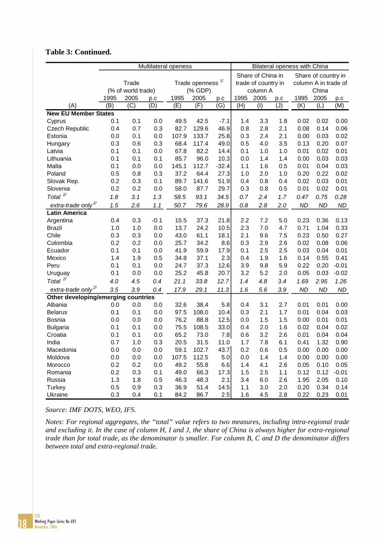
Table 3: Continued.

1995 2005 p.c 1995 2005 p.c 1995 2005 p.c 1995 2005 p.c(A) (B) (C) (D) (E) (F) (G) (H) (I) (J) (K) (L) (M)

New EU Member StatesCyprus 0.1 0.1 0.0 49.5 42.5 -7.1 1.4 3.3 1.8 0.02 0.02 0.00Czech Republic 0.4 0.7 0.3 82.7 129.6 46.9 0.8 2.8 2.1 0.08 0.14 0.06Estonia 0.0 0.1 0.0 107.9 133.7 25.8 0.3 2.4 2.1 0.00 0.03 0.02Hungary 0.3 0.6 0.3 68.4 117.4 49.0 0.5 4.0 3.5 0.13 0.20 0.07Latvia 0.1 0.1 0.0 67.8 82.2 14.4 0.1 1.0 1.0 0.01 0.02 0.01Lithuania 0.1 0.1 0.1 85.7 96.0 10.3 0.0 1.4 1.4 0.00 0.03 0.03Malta 0.1 0.0 0.0 145.1 112.7 -32.4 1.1 1.6 0.5 0.01 0.04 0.03Poland 0.5 0.8 0.3 37.2 64.4 27.3 1.0 2.0 1.0 0.20 0.22 0.02Slovak Rep. 0.2 0.3 0.1 89.7 141.6 51.9 0.4 0.8 0.4 0.02 0.03 0.01Slovenia 0.2 0.2 0.0 58.0 87.7 29.7 0.3 0.8 0.5 0.01 0.02 0.01Total 2/ 1.8 3.1 1.3 58.5 93.1 34.5 0.7 2.4 1.7 0.47 0.75 0.28 extra-trade only 2/ 1.5 2.6 1.1 50.7 79.6 28.9 0.8 2.8 2.0 ND ND NDLatin AmericaArgentina 0.4 0.3 -0.1 15.5 37.3 21.8 2.2 7.2 5.0 0.23 0.36 0.13Brazil 1.0 1.0 0.0 13.7 24.2 10.5 2.3 7.0 4.7 0.71 1.04 0.33Chile 0.3 0.3 0.0 43.0 61.1 18.1 2.1 9.6 7.5 0.23 0.50 0.27Colombia 0.2 0.2 0.0 25.7 34.2 8.6 0.3 2.9 2.6 0.02 0.08 0.06Ecuador 0.1 0.1 0.0 41.9 59.9 17.9 0.1 2.5 2.5 0.03 0.04 0.01Mexico 1.4 1.9 0.5 34.8 37.1 2.3 0.4 1.9 1.6 0.14 0.55 0.41Peru 0.1 0.1 0.0 24.7 37.3 12.6 3.9 9.8 5.9 0.22 0.20 -0.01Uruguay 0.1 0.0 0.0 25.2 45.8 20.7 3.2 5.2 2.0 0.05 0.03 -0.02Total 2/ 4.0 4.5 0.4 21.1 33.8 12.7 1.4 4.8 3.4 1.69 2.95 1.26 extra-trade only 2/ 3.5 3.9 0.4 17.9 29.1 11.3 1.6 5.6 3.9 ND ND NDOther developing/emerging countriesAlbania 0.0 0.0 0.0 32.6 38.4 5.8 0.4 3.1 2.7 0.01 0.01 0.00Belarus 0.1 0.1 0.0 97.5 108.0 10.4 0.3 2.1 1.7 0.01 0.04 0.03Bosnia 0.0 0.0 0.0 76.2 88.8 12.5 0.0 1.5 1.5 0.00 0.01 0.01Bulgaria 0.1 0.1 0.0 75.5 108.5 33.0 0.4 2.0 1.6 0.02 0.04 0.02Croatia 0.1 0.1 0.0 65.2 73.0 7.8 0.6 3.2 2.6 0.01 0.04 0.04India 0.7 1.0 0.3 20.5 31.5 11.0 1.7 7.8 6.1 0.41 1.32 0.90Macedonia 0.0 0.0 0.0 59.1 102.7 43.7 0.2 0.6 0.5 0.00 0.00 0.00Moldova 0.0 0.0 0.0 107.5 112.5 5.0 0.0 1.4 1.4 0.00 0.00 0.00Morocco 0.2 0.2 0.0 49.2 55.8 6.6 1.4 4.1 2.6 0.05 0.10 0.05Romania 0.2 0.3 0.1 49.0 66.3 17.3 1.5 2.5 1.1 0.12 0.12 -0.01Russia 1.3 1.8 0.5 46.3 48.3 2.1 3.4 6.0 2.6 1.95 2.05 0.10Turkey 0.5 0.9 0.3 36.9 51.4 14.5 1.1 3.0 2.0 0.20 0.34 0.14Ukraine 0.3 0.4 0.1 84.2 86.7 2.5 1.6 4.5 2.8 0.22 0.23 0.01

Trade openness 1/

(% GDP)Trade

(% of world trade)


column A

Share of country in column A in trade of

China

Multilateral openess Bilateral openess with China

Source: IMF DOTS, WEO, IFS.

Notes: For regional aggregates, the “total” value refers to two measures, including intra-regional trade and excluding it. In the case of column H, I and J, the share of China is always higher for extra-regional trade than for total trade, as the denominator is smaller. For column B, C and D the denominator differs between total and extra-regional trade.


39ECB


European Central Bank Working Paper Series

For a complete list of Working Papers published by the ECB, please visit the ECB’s website(http://www.ecb.int)

665 “The euro as invoicing currency in international trade” by A. Kamps, August 2006.

666 “Quantifying the impact of structural reforms” by E. Ernst, G. Gong, W. Semmler andL. Bukeviciute, August 2006.

667 “The behaviour of the real exchange rate: evidence from regression quantiles” by K. Nikolaou,August 2006.

668 “Declining valuations and equilibrium bidding in central bank refinancing operations” byC. Ewerhart, N. Cassola and N. Valla, August 2006.

669 “Regular adjustment: theory and evidence” by J. D. Konieczny and F. Rumler, August 2006.

670 “The importance of being mature: the effect of demographic maturation on global per-capitaGDP” by R. Gómez and P. Hernández de Cos, August 2006.

671 “Business cycle synchronisation in East Asia” by F. Moneta and R. Rüffer, August 2006.

672 “Understanding inflation persistence: a comparison of different models” by H. Dixon and E. Kara,September 2006.

673 “Optimal monetary policy in the generalized Taylor economy” by E. Kara, September 2006.

674 “A quasi maximum likelihood approach for large approximate dynamic factor models” by C. Doz,D. Giannone and L. Reichlin, September 2006.

675 “Expansionary fiscal consolidations in Europe: new evidence” by A. Afonso, September 2006.

676 “The distribution of contract durations across firms: a unified framework for understanding andcomparing dynamic wage and price setting models” by H. Dixon, September 2006.

677 “What drives EU banks’ stock returns? Bank-level evidence using the dynamic dividend-discountmodel” by O. Castrén, T. Fitzpatrick and M. Sydow, September 2006.

678 “The geography of international portfolio flows, international CAPM and the role of monetarypolicy frameworks” by R. A. De Santis, September 2006.

679 “Monetary policy in the media” by H. Berger, M. Ehrmann and M. Fratzscher, September 2006.

680 “Comparing alternative predictors based on large-panel factor models” by A. D’Agostino andD. Giannone, October 2006.

681 “Regional inflation dynamics within and across euro area countries and a comparison with the US”by G. W. Beck, K. Hubrich and M. Marcellino, October 2006.

682 “Is reversion to PPP in euro exchange rates non-linear?” by B. Schnatz, October 2006.

683 “Financial integration of new EU Member States” by L. Cappiello, B. Gérard, A. Kadareja andS. Manganelli, October 2006.


684 “Inflation dynamics and regime shifts” by J. Lendvai, October 2006.

685 “Home bias in global bond and equity markets: the role of real exchange rate volatility”by M. Fidora, M. Fratzscher and C. Thimann, October 2006

686 “Stale information, shocks and volatility” by R. Gropp and A. Kadareja, October 2006.

687 “Credit growth in Central and Eastern Europe: new (over)shooting stars?”by B. Égert, P. Backé and T. Zumer, October 2006.

688 “Determinants of workers’ remittances: evidence from the European Neighbouring Region”by I. Schiopu and N. Siegfried, October 2006.

689 “The effect of financial development on the investment-cash flow relationship: cross-countryevidence from Europe” by B. Becker and J. Sivadasan, October 2006.

690 “Optimal simple monetary policy rules and non-atomistic wage setters in a New-Keynesianframework” by S. Gnocchi, October 2006.

691 “The yield curve as a predictor and emerging economies” by A. Mehl, November 2006.

692 “Bayesian inference in cointegrated VAR models: with applications to the demand foreuro area M3” by A. Warne, November 2006.

693 “Evaluating China’s integration in world trade with a gravity model based benchmark”by M. Bussière and B. Schnatz, November 2006.

ISSN 1561081-0

9 7 7 1 5 6 1 0 8 1 0 0 5

Documents

Evaluating China's integration in world trade with a gravity model