The Vodka is Potent, but the Meat is Rotten1: Evaluating Measurement Equivalence across Contexts

Zachary Elkins Department of Government University of Texas at Austin

zelkins@austin.utexas.edu

John Sides Department of Political Science George Washington University

jsides@gwu.edu

June 2010

Abstract

Valid measurement in comparative research depends on the equivalence of constructs and indicators across contexts, but thus far the pace of comparative research has outstripped attention to measurement equivalence. We describe different types and sources of equivalence, as well as methods of diagnosing non-equivalence. We emphasize the need to develop and test theories about threats to equivalence. We derive hypotheses about non-equivalence related to two concepts, democracy and development. Our empirical tests of items measuring these concepts demonstrate non-equivalence, though of differing magnitude and form. We conclude with general guidelines for the prevention, diagnosis, and treatment of non-equivalence.

1 Russian (mis)translation of “The spirit is strong but the flesh is weak,” from a cross-national survey item (Smith 2003).

Scholars of comparative politics continue to venture into more and more jurisdictions across longer

stretches of time. Some cross-national datasets contain the universe of independent states since 1800, and

cross-national survey projects now include much of the developed and developing worlds. The benefits of

this expansion are clear: added cases can produce more variation in variables of interest, provide more

powerful tests of extant theory, and illuminate empirical puzzles that lead to new theories. However,

comparative inquiry grinds to halt if scholars cannot develop comparable concepts and measures across

diverse national and historical contexts. This is true whether the purpose of comparative inquiry is

descriptive or inferential. If an observed attribute is a product of not only the underlying construct but also

a measurement irregularity particular to time or place, then inferences are compromised. Thus the

importance of equivalent measurement, the challenge we address in this paper.2

Concern about measurement non-equivalence is not new. Most of chapter 2 of The Civic Culture, for

example, seeks to justify the equivalence of the authors’ measures (Almond and Verba 1963; see also

Anderson 1967; Przeworski and Teune 1966; Rokkan, Verba, Viet, and Almasy 1969). But since the initial

waves of large-scale comparative projects, the problem of equivalence has receded to the background for

most political scientists. There are important exceptions, including van Deth’s (1998) volume, Adcock and

Collier’s (2001) guidance on measurement validity and equivalence, Bartels’ (1996) work on pooling

disparate observations, Brady’s (1985, 1989) work on interpersonal incomparability, and King and co-

authors’ work on anchoring vignettes (King et al. 2004; King and Wand 2007). Measures of a handful of

concepts have been subject to formal tests of equivalence.3 Nonetheless, we suspect that most analysts of

secondary data set aside concerns about non-equivalence, choosing (understandably) to attend to issues

directly under their control, such as estimation and model specification.

Our central message is that scholars can benefit from thinking more theoretically and systematically

about when and how non-equivalence arises. We begin by delineating some common threats to equivalent

measurement as researchers traverse both time and space. We then conceptualize the various forms that 2 The terms “equivalence,” “invariance,” and “comparability” are often used synonymously in the literature. 3 These concepts include human values (Davidov, Schmidt, and Schwartz 2008), nationalism and patriotism (Davidov 2009), political efficacy (King et al. 2004), and social capital (Paxton 1999).

1

non-equivalence takes. We develop and test hypotheses of non-equivalence in the context of two important

concepts in comparative politics: democracy and economic development. In so doing, we demonstrate how

analysts can establish the presence of non-equivalence using both descriptive and inferential techniques.

Finally, we offer suggestions for analysts using cross-national and over-time data. Sound advice for

addressing non-equivalence is scattered across treatments of conceptualization and measurement (e.g.,

Adcock and Collier 2001; King et al. 2004; van Deth 1998). We assemble a set of guidelines for how

scholars can prevent, diagnose, and treat non-equivalence.

Ours is not an account that identifies a methodological sin and then promises a path to redemption.

Many problems of non-equivalence cannot be simply corrected, but are endemic to the comparative

enterprise. We seek instead to specify ways by which scholars can think about and test for non-equivalence.

Moreover, we do not conceive of non-equivalence as original sin. It challenges comparative inquiry, but

does not doom the very possibility of comparison. Rather, confronting and engaging non-equivalence will

render comparative analyses more persuasive.

Space, Time, and Non-Equivalence: The Woods-Jordan Problem and the Bonds-Ruth Problem

Thinking theoretically about non-equivalence requires accounting for its many sources. One could

typologize threats to non-equivalence in different ways—e.g., by the stages of the conceptualization and

measurement process (see van Deth 2009). For the purpose of illustration, it is enough to conceive of these

threats in terms of the two basic contextual dimensions of comparative inquiry: time and space.

The Woods-Jordan Problem: Non-equivalence across Space

Who is the better athlete: Tiger Woods or Michael Jordan? The New York Times (2008) ran a widely

circulated online debate on the topic not long ago. The question has no straightforward answer because

Woods and Jordan played different sports, and the talents needed to excel in one sport are less relevant in

the other. Woods does not need a jump shot. Jordan does not need a flop shot. Some measures have this

same problem: they do not travel well from one location to another. These dislocating effects arise from

differences across contexts in language, custom, and culture—that is, shared meanings, norms, and values.

2

Non-equivalence can emerge across countries, other jurisdictional units, ethnic groups, social classes, or any

set of entities defined by cultural, political, or economic markers.

Various manifestations of non-equivalence across countries emerge just within survey research.

Most obviously—as our title emphasizes—there is the difficulty of constructing equivalent survey items in

different languages (e.g., Anderson 1967; Blais and Gidengil 1993; Drasgow and Probst 2005; Iyengar 1976).

Moreover, the very manner of data collection may engender different reactions in different cultures. As

Verba (1969) notes, the act of providing opinions about political issues to a complete stranger may prove

unremarkable in some cultures but foreign in others. At a deeper level, culturally specific values may imply

varying “response styles.” For instance, a collectivist orientation is more evident in East Asian countries

and is associated with providing socially desirable responses (Lalwani, Shavitt, and Johnson 2006).

Response styles affect not only survey respondents but any actor charged with producing data. Herrera and

Kapur (2007: 378) note that measuring “targets” (e.g., stated goals of governments) can lead to bias: “When

targets are ceilings (such as fiscal deficits), the data are likely to have downward bias. When targets are

floors (such as social sector indicators), the data are likely to be biased upward.”

One may also observe the “Woods-Jordan” problem when employing a measure across groups

within geographic boundaries, such as groups defined by gender, ethnicity, and religion. These

characteristics create non-equivalence because group members are exposed to particular experiences, ideas,

and expectations, and learn to act and think in distinct ways. To approach different groups—even groups

that are literal neighbors—with a common set of measures may be no different from taking those measures

into different countries. These kinds of group differences underlie the concern about the validity of

educational testing across racial and ethnic groups. One political science example concerns the gender gap

in knowledge of politics. Mondak and Anderson (2004) argue that this gap arises in part because men are

more likely to guess, rather than admit that they do not know, when asked questions about their knowledge.

Another example involves equivalence across political institutions within a single country. Often

scholars want to measure some attribute of actors in these institutions, but lack any common measures.

The most noteworthy example involves ideology. Scholars of American politics want to know the

3

ideological preferences of elected and appointed leaders: the President, Senators, House members, Supreme

Court Justices, other federal judges, etc. But the President does not vote on all of the bills that members of

Congress vote on. Senators and representatives also vote on different bills. Judges and justices consider

cases and not bills, but not always the same set of cases, given the geographical stratification of federal

district and appellate courts. These challenges have led scholars to pursue different strategies, including the

use of bridge observations, or actors within one institution who have served in another institution or taken

positions on issues confronting another institution (Bailey 2007; Poole 1998)

A final dimension of cross-sectional non-equivalence lies at the level of the individual, regardless of

her context. Individuals have distinct values, orientations, and reference points that may affect their

responses to measurement instruments, such as surveys (see Brady 1985). Non-equivalence may also arise

because of an individual’s interaction with the survey interviewer. Those interactions vary in how much

rapport the interviewer and respondent develop, how well they communicate with each other, and thus in

the quality and content of the response provided (see Suchman and Jordan 1990). Interviewers are, of

course, trained to minimize idiosyncrasies by adhering to protocols. And yet rigid adherence to a protocol

could itself create non-equivalence if additional information from the interviewer would enable the

respondent to understand and answer the question in the manner intended. “Individualized” non-

equivalence is probably the source least explored.

The Bonds-Ruth Problem: Non-equivalence across Time

Is Barry Bonds the best home run hitter in the history of Major League Baseball? Measured by the

raw number of home runs, he is. But is it appropriate to compare Bonds’ performance with that of players

whose careers occurred years or even decades ago? Many things have changed in baseball since the era of

Babe Ruth or even Hank Aaron: the size of ballparks, the quality of pitching, the composition of baseballs

and bats, and the apparent prevalence of steroid use. In short, times have changed, and the question is

whether they have changed so much as to render “number of career home runs” a misleading measure for

4

comparing the prowess of hitters over the history of baseball. This is the “Bonds-Ruth problem,” with a

nod towards the countless other intergenerational rivals who have featured in barroom arguments.

To date, much research on equivalence is concerned with space rather than time—with Jordan and

Woods, rather than Bonds and Ruth (but see Bailey 2007 and Paxton 2009). But as data collection persists

in the social science, the passage of time can change the meaning of constructs and the items used to

measure them. Such changes may stem from events, shifts in cultural norms, and the like (see Clarke et al.

1999; Reus-Smit 1997). As time passes, researchers may need to re-conceptualize the construct—e.g.,

“What does it now mean to be X?”—and reconsider whether particular items tap that construct.

One example concerns prejudice toward African-Americans. Many indicators suggest that prejudice

has declined over time: fewer white Americans oppose interracial marriage, integrated schools, and other

kinds of social interactions with blacks, and fewer Americans believe that blacks are innately inferior,

especially with regard to intelligence (see Schuman et al. 1997). At the same time, other scholars have

argued that these changes do not necessarily indicate a less prejudiced public because the nature of racism

itself has changed to one that (and here we simplify) emphasizes lack of effort rather than lack of ability, a

notion called symbolic racism (Sears 1988) or racial resentment (Kinder and Sanders 1996). This argument

has met vigorous resistance (e.g., Sniderman and Tetlock 1986). Ultimately, the debate boils down to

questions about equivalence. Is the prejudice of yesterday the same as the prejudice of today? Are new

indicators needed to capture prejudice today? If so, how does that complicate comparisons over time?4

A second example involves the measurement of poverty. Is the rate of poverty in a particular

country higher today than in years past? This proves to be a complicated question. Accounting for

inflation is only one threat, and even that is not perfectly measurable. Over time, the poverty threshold

itself may need adjustment, if median income has changed. The monies that are defined as “income” may

need adjustment if certain social welfare transfers have been created or eliminated in the intervening years.

4 The same set of issues confronts the study of political tolerance (see Mondak and Sanders 2003; Nunn, Crockett, and Williams 1978; Sullivan, Pierson, and Marcus 1982). Why has tolerance of such groups as atheists, communists, and socialists increased? Because the public has come to support extending liberties even to unpopular groups, or because the groups themselves have become less unpopular?

5

The tax burden may also have changed, such that less or more income is being paid in taxes. All of these

problems led to a new proposed standard for poverty in the United States in 1995 (see Betson and Warlick

1998).5 In general, differing approaches to the measurement of poverty can lead to drastically different

conclusions about the trend (see Jorgenson 1998; Triest 1998).

Both cases demonstrate that measurement equivalence may not only stop at the border, but also

vary over time. The meaning of constructs changes, as does the relevance of particular measures. Although

the example of prejudice involves decay, this is not the only “functional form” that could describe the

relationship between time and equivalence. Discrete events such as crises or elections may also render

certain measures more or less equivalent, perhaps only temporarily so. Thus, “local” knowledge—long

appreciated in comparative politics—is also central to the study of “politics over time.”

Conceptualizing Equivalence

These various threats have predictable symptoms in empirical research. We can conceptualize the

forms of non-equivalence in terms of the parameters of the traditional measurement model (see Bollen 1989:

17). Suppose that a unit i (an individual, country, etc.) has an observed value (xi) for some indicator, which

is linearly related to the underlying, unobserved (latent) attribute (ξ). The strength of the relationship

between the latent attribute and the observed indicator is captured by a parameter λ, often called the factor

loading. The observed value of x also depends on a “uniqueness” parameter (δ). An intercept term μ, is the

value of x when the latent attribute is equal to 0. To capture the notion of equivalence, imagine two

equations, one for “Context 1” and another for “Context 2,” with respective subscripts.

xi1= μ1+λ1ξi1+δi1 (1)

xi2= μ2+λ2ξi2+δi2 (2)

If the contexts were countries, an important goal would be to use the values of x in Countries 1 and 2 to

make inferences about how much the latent attribute varies across countries. If the contexts represented

5 Poverty measures may also exhibit cross-sectional non-equivalence (i.e., the Woods-Jordan problem), if, for example, they fail to account for variation in the cost of living in different parts of a country.

6

time periods, then the parallel goal would be to make inferences about variation across time. Either task

depends on equivalence in measurement. Equivalence can be conceived in hierarchical terms, starting with

the fundamental forms and moving to the more subtle, with each form depending on equivalence at the

prior level. We discuss three forms of equivalence: construct, structural, and scalar.

Most fundamentally, a construct should have a similar meaning in each context. This construct

equivalence (Van de Vijver 2003)—or conceptual equivalence (Hui and Triandis 1985)—pertains to

conceptualization and even case selection, both of which precede operationalization and measurement. If

construct equivalence does not hold, then the latent attributes in equations (1) and (2) are essentially

different; instead of ξ1 and ξ2, the attributes are really ϕ1 and ξ2—i.e., apples and oranges. Construct non-

equivalence would arise when measuring attitudes towards authoritarian rule in societies that have

experienced only democracy, the strength of party organizations where parties are banned, or even aspects

of written constitutions in countries that have an unwritten body of higher law or a patchwork of basic laws.

Many concepts are essentially contested (Gallie 1956). as is their application to particular contexts.

Construct equivalence is fundamentally determined by contestation within a community of scholars who

evaluate whether a construct has a similar meaning in various contexts. Some cases of construct non-

equivalence may be widely agreed upon, such as the measurement misadventures identified as “conceptual

stretching” (Sartori 1971; Collier and Levitsky 1997). More often, scholars will disagree about whether a

concept has been stretched too far. Below we examine such a debate: whether the concept of democracy is

portable from the developing democracies of the global “South” to the post-Soviet states of the “East.”

One solution to construct non-equivalence is to climb the “ladder of abstraction” (Sartori 2008

[1971]) by redefining the construct as something broader and perhaps more applicable to different contexts.

In the case of constitutions, one could use a concept such as “higher law,” which does not presuppose any

sort of legal form. The other solution, of course, is to retain the construct but avoid measuring it where it is

meaningless or hopelessly stretched. This may entail delimitations in the data under consideration.

7

Although construct equivalence is of the utmost importance, it cannot be evaluated in any strict

empirical sense, although its violation will be apparent in tests of more subtle forms of equivalence.

Construct equivalence is best evaluated through careful conceptualization that is guided by theory and

grounded in detailed knowledge about particular countries or cultures—criteria that are themselves subject

to debate. Given its contingent nature, we do not address construct equivalence in much depth, focusing

instead on measurement, although evaluating construct equivalence remains an important task.

A second kind of equivalence is structural equivalence, in which the latent construct has a similar

“architecture” across contexts.6 The question is how well the observed indicators that measure the concept

in one context overlap with those that do so in another context. 7 At the extreme, a concept may have a

unique empirical manifestation in one context, in which case no indicators of that construct elsewhere

would be relevant. In other cases, a set of indicators may introduce surplus meaning where or when the

construct takes on a narrower meaning or, conversely, may fail to capture a construct’s multiple dimensions.

Assume that a concept is measured with a five-indicator scale administered in two contexts. In

equations (1) and (2) xi is replaced with a 5×1 vector of indicators (X) that is related to the same latent

attribute (ξ) by a vector of loadings (Λ) and a vector of uniqueness parameters (δ):

X1= μ1+Λ1ξ1+δ1 (3)

X2= μ2+Λ2ξ2+δ2 (4)

Assume that in the first context, each of the indicators in X1 is a valid indicator of the latent attribute ξ1.

Structural equivalence would not obtain if, for example, any of the indicators in X2 is not in fact an indicator

of the latent attribute ξ2. The same is true if the indicators in X2 are actually indicators of two distinct

factors rather than a single factor—in other words, if the latent attribute ξ2 is multi-dimensional in the

6 Similar notions appear elsewhere: Cheung and Rensvold’s (2000) “factor form invariance,” Stark, Chernyschenko, and Drasgow’s (2006) “configural invariance,” and Bollen’s (1989: 356) “model form” invariance. 7 Construct non-equivalence and structural non-equivalence will likely go hand-in-hand much of the time. (Van de Vijver and Leung (1997:8-9) actually treat construct and structural equivalence as the same thing.) However, it is possible that a construct means the same thing in various contexts but that the “structural” relationship between that construct and a set of indicators differs across contexts.

8

second context but not the first. Przeworski and Teune’s (1966) distinction between “equivalent” and

“identical” items is instructive here, even though their terms differ from modern usage (Przeworski and

Teune refer to functional equivalence, not strict measurement equivalence). They suggest that items do not

have to be “identical” (i.e., exactly the same) across contexts, as long as they capture the same basic

phenomenon. In their example, a measurement model of political activity in the United States that uses an

indicator such as “giving money to campaigns” might be functionally “equivalent” but not “identical” (in

their sense of those terms) to a model in Poland that substituted “volunteer for social works” for the

campaign item. Nevertheless, to return to the standard usage of “equivalent,” the measurement model

across these contexts would not be structurally equivalent because the architecture of indicators differs.

This is not intrinsically a flaw, of course: context-specific indicators may enhance construct equivalence.

But they must be used and evaluated carefully. We return to this point below.

Structural non-equivalence need not reflect an entirely different model form across contests. It may

more often be a matter of degree: in different contexts, the strength of the relationship between indicators

and a construct could vary. In terms of equations (3) and (4), strict structural equivalence means that Λ1=Λ2;

that is, the factor loadings are equivalent.8 This type of equivalence is linked with the concept of differential

item functioning (DIF), about which there is a large literature in educational testing (see Angoff 1993 for an

introduction and King et al. 2004 for a political science application). In educational testing, DIF means that

two students of equal aptitude have different probabilities of answering the same test question correctly (e.g.,

because the question contains a cultural bias). More generally, structural non-equivalence could mean, for

instance, that one of the observed indicators is strongly associated with the latent attribute in one context,

but only weakly associated with the attribute in the other context.

Structural non-equivalence surfaces in Canache, Mondak, and Seligson’s (2001) study of the

standard “satisfaction with democracy” survey item. They find that this indicator taps multiple

8 Cheung and Rensvold (2000) refer to this property as “factorial invariance.” Stark, Chernyshenko, and Drasgow (2006) call it “metric equivalence.” We do not separate structural and metric equivalence because their border can be murky. For example, an extreme case of apparent metric non-equivalence might be better understood as structural non-equivalence.

9

dimensions—satisfaction with the current political system, satisfaction with incumbent political authorities,

and support for democracy—and that its relationship to these dimensions varies across countries. For

example, “satisfaction with democracy” is strongly associated with system support in Uruguay but not so in

Costa Rica. In a study of system support, then, the item “satisfaction with democracy” would exhibit

structural non-equivalence because of its near-irrelevance in the Costa Rican context.

A third form of equivalence is scalar equivalence (Cheung and Rensvold 2000; Stark, Chernyshenko,

and Drasgow 2006). Whereas structural equivalence involves the slopes in the measurement model, scalar

equivalence means that the “intercepts”—i.e. the value of the observed indicator when the latent attribute is

0—are equivalent across countries. Scalar non-equivalence means that observed values in one context are

systematically higher or lower than in another context, even when the value of the latent attribute and the

factor loadings are the same across contexts. This could arise, for example, if the tendency to agree to

survey questions (acquiescence response style) differed across contexts or groups (e.g., Bachman and

O’Malley 1984; Johnson et al. 2005). If the denizens of one country are more likely to be yea-sayers, then

on average they will appear “higher” on a given indicator relative to respondents other countries.

Scalar non-equivalence could also arise if respondents in different contexts have different “reference

points” in mind when they evaluate themselves. For example, when asked to indicate their affect toward

social groups, some people tend to assign higher, or “hotter,” scores regardless of the group (Wilcox,

Sigelman, and Cook 1989). Thus, the purpose of anchoring vignettes is to locate, or “anchor,” respondents

to a common reference point by asking them to evaluate the individuals described in the vignettes as well as

themselves (King et al. 2004). A national-level example of this problem, and one we investigate below,

involves Polity’s standard measure of democracy (Marshall, Jaggers, and Gurr 2004). The United States has

scored the maximum of 10 on Polity’s measure of democracy since the Civil War. But is a 10 during the

height of Jim Crow or the years prior to women’s suffrage equivalent to a 10 in 2000? Almost undoubtedly

not, unless one discounts the inclusion of women and minorities in the political process. There appears to

be a serious problem of deflation in the Polity measure that requires adjustment.

10

These three types of equivalence draw our attention to the complexities of measurement across

contexts and to the potential difficulties when equivalence does not hold. 9 In particular, non-equivalence

may confound both descriptive and causal inference. For example, it may complicate efforts to use context-

level averages to discern the true effect of context on the attribute in question. The analogous situation in

educational testing is “differential test functioning” (DTF), which results from the systematic biases created

by differential item functioning. In such cases, the true effect of group membership on the test score, also

known as the “impact,” is confounded by DIF. Only if differentially functioning indicators have off-setting

biases, with some “favoring” one group and some “favoring” others, will DIF fail to create DTF.

Non-equivalence affects not only the estimated means of attributes, but also the relationships

among those attributes. Brady (1985) shows that both structural and scalar non-equivalence can bias

estimates of the relationship between observed indicators. For example, non-equivalence is just as

important for understanding the relationship between democracy and economic development as it is for

comparing mean levels of each attribute. Standard procedures in the analysis of cross-contextual data—

which typically entail taking well-known indicators (e.g., Polity democracy scores) “off the shelf,” or

selecting a set of indicators and constructing a summary scale, perhaps with minimal diagnostics within each

context to assess dimensionality (via exploratory factor analysis) or reliability (e.g., an alpha statistic)—are

not sufficient to ensure valid and reliable measurement.

Approaches to Diagnosing Non-Equivalence

Diagnosing non-equivalence can involve both descriptive and inferential techniques. Descriptive

techniques are valuable simply because they enable researchers to “see” any apparent differences across

contexts, which may then in turn inspire theorizing about the sources of these differences and then possibly

formal tests of their significance. The simplest means of diagnosis is simply to estimate a separate

9 One can also test for the equivalence of other parameters in the measurement model, such as measurement error variance and the means of and covariances among the latent variables. But these are arguably less crucial than other kinds of non-equivalence (Stark, Chernyshenko, and Drasgow 2006: 1293).

11

measurement model for each contextual unit and then examine the relevant parameters. Graphical

representations may be particularly helpful, as we demonstrate below.

For the purposes of inference, two data-analytic frameworks are commonplace: structural equation

modeling (SEM) and item response theory (IRT).10 These approaches, and the specific methods within

them, have largely developed in parallel literatures. IRT evolved within educational testing (Lord and

Novick 1968), while SEM developed in psychometrics more generally. Despite their different origins, they

are similar in many respects. (We describe and compare them in the on-line appendix). We conclude that

their differences are largely terminological and notational, with one unit-of-measurement assumption

separating the two. Given the data in question, the empirical analysis below draws on SEM. The chief

liability of both methods is, however, an important one: both are employed when there are multiple

indicators of the construct in question. When there are not, these techniques are less helpful. In the

conclusion we address the challenge of constructing a single measure that is equivalent across contexts.

Whether one is working in an IRT or SEM framework, typical tests for equivalence follow the same

logic. A researcher conducts a hierarchical series of tests that probe for finer degrees of incomparability

(Bollen 1989; Cheung and Rensvold 2000). We describe three specific tests based on the forms of

equivalence. First, does the same measurement model apply equally well in different contexts (a broad test

of structural equivalence)? This test entails pooling the different contexts and estimating an

“unconstrained” model that allows all of the model’s parameters to vary across contexts—with the

exception of the indicator whose loading is scaled to 1 for the purposes of identification, and one of the

intercepts, which must also be constrained equal across groups (see Bollen 1989: 307). If the fit of this

model is adequate, then the basic architecture of the model is assumed to be equivalent across contexts and

this model becomes the baseline against which all constrained models are evaluated. If this condition does

not hold, then the model is poorly specified in some, if not all, contexts and one need go no further, as

subsequent tests all assume a measurement model that fits the data and whose basic architecture is

10 SEM is also called “covariance structure modeling” or as “mean and covariance structure modeling.”

12

equivalent across contexts. Eyeballing the parameter estimates across contexts will provide an initial sense

of where and why any non-equivalence arises.

Second, provided that the model fit in each context is adequate, one can then test for milder

symptoms of structural equivalence: namely, whether the individual loadings differ in magnitude across

contexts. This question can be tested first with an overall or “global” test of structural equivalence,

constraining all loadings to be equal across contexts, again with a single indicator’s loading set to 1 for the

purposes of scaling.11 If the fit of the model is poor, one can pursue the offending indicator(s) by testing

the equivalence of individual loadings. However, these tests encounter a “standardization problem”

(Rensvold and Cheung 2001). In short, selecting a scaling indicator assumes that this indicator is itself

equivalent. If this assumption is not true, then there is a much higher probability of a Type I error, or

mistakenly rejecting the null of equivalence (Stark, Chernyshenko, and Drasgow 2006: 1304). Rensvold and

Cheung (2001) propose a sequence of models that vary the combination of the scaling indicator (or

“referent”) and the indicator (the “argument”) whose loading is constrained across contexts.12 If this form

of structural equivalence cannot be established, the remedies will depend on the number and nature of

available indicators. Researchers could pursue a model that is “partially” equivalent, constraining some

factor loadings to be equal across contexts and allowing others to vary (see Byrne, Shavelson, and Muthén

1989). Or researchers may instead choose to eliminate certain (non-equivalent) indicators. Ultimately, there

is no one default “solution.” We return to this subject below.

Third, if structural equivalence has been established then one may go on to evaluate scalar

equivalence. That is, do different contexts share a common origin on each indicator, i.e., the value of the

11 In models with more than one factor, it may also be instructive to conduct subsequent tests of global metric equivalence at the level of each individual factor (Rensvold and Cheung 2001: 36). 12 A model is estimated for each possible pairing of referent and argument—e.g., in a three-indicator model, indicators 1 and 2, 2 and 3, and 1 and 3. If any model’s fit is worse than the unconstrained model, then that pair of indicators is flagged. The set of equivalent items is identified by eliminating any feasible set that includes a flagged pair. If 1-2 is the flagged pair, then the only feasible set is 2-3, since 1-2 and 1-2-3 are eliminated. If no such pairs are flagged, then metric equivalence has been established. In general, in an N-indicator model, there are N(N-1)/2 pairs of indicators. The number of feasible subsets of items is a more complicated formula, but the upshot is that the number of subsets grows larger with additional indicators. See Rensvold and Cheung (2001) for strategies on dealing with models that have many indicators.

13

indicator when the latent construct is 0? Evaluating scalar equivalence entails a similar test constraining the

intercepts to be equal across contexts. In many examples, the series of tests stops here, although

researchers can also test for equivalence in measurement error variance or any other parameter of the model.

In estimating this series of models, each constrained model is compared against the fully

unconstrained model according to various measures of fit. A standard measure in SEM is the chi-squared

statistic. A significant chi-squared statistic indicates that there is not a close fit between the data and the

model’s predictions. One can test for equivalence by calculating the change in the chi-squared values across

nested models to see if imposing constraints significantly worsens the fit. The difference in two chi-squared

statistics also follows the chi-squared distribution, with degrees of freedom equal to the difference in the

two models’ degrees of freedom. A well-known problem with the chi-squared statistic and with the

difference between two chi-squared statistics is that large samples are more likely to produce significant chi-

squared statistics. Even in these cases, calculating the difference in the chi-squared is useful, as there is no

other fit index whose difference between two models follows a known distribution (Rensvold and Cheung

2001). Nevertheless, it is important to draw upon multiple indicators of fit. We draw on three other

indicators: the Tucker-Lewis Index (TLI), the Comparative Fit Index (CFI), and the root mean squared

error (RMSEA). For the TLI and CFI, values close to 1 indicate a good fit. For the RMSEA, values close

to 0 indicate a good fit (see Browne and Cudeck 1993).

Two Assessments of Equivalence: Democracy and Development

To what degree is non-equivalence manifest in measures of political science constructs? For two

constructs, democracy and development, we develop theoretical expectations of non-equivalence along both

spatial and temporal dimensions, and thus identify the potential for both Woods-Jordan problems and

Bonds-Ruth problems. We then evaluate items used to measure those constructs using the methods

described above. We determine which, if any, items “function” differently across different contexts, explore

the reasons why these items function differently; and, in one case, examine the consequences of including or

14

removing these items. The two constructs are measured at the country level, which allows us to explore

non-equivalence outside the realm of survey research, where equivalence has been considerably more central.

Democracy across Time

To investigate the equivalence of democracy measures, we first consider a potential manifestation of

the Bonds-Ruth problem: whether measures of democracy are equivalent across time and, in particular,

across “waves.” Some properties of common democracy measures have been scrutinized (see, e.g., Munck

2009; Treier and Jackman 2007; Gleditsch and Ward 1997), but there has been less attention to the

equivalence of these measures across time, even as scholars have taken an explicitly historical view of

democracy, sometimes attempting to periodize its temporal variation (e.g., Huntington 1991). Measures of

democracy that presuppose certain institutional arrangements and practices may not travel well across time.

Another problem concerns reference points: should we measure democracy against a single

standard or against the standard at the time, e.g., by constructing context-adjusted measures (Adcock and

Collier 2001)? The issue is analogous to inflation in measures based on currency, like GDP per capita. As

noted before, the United States has scored the maximum 10 on Polity’s democracy scale since the Civil War.

For much of this period, however, significant portions of the population (especially women and blacks)

were excluded from voting. Assuming a single (non-contextualized) standard, the Polity participation scores

before women and blacks earned the de jure and de facto right to vote must be inflated and, it seems,

incomparable to contemporary scores in an absolute sense (Johnson 1999).

Vanhanen’s (2000) measures of democracy, on the other hand, proceed from the opposite

assumption. Vanhanen proposes two objective indicators—turnout and the winning party’s margin of

victory—that ostensibly tap participation and competition, two central dimensions of democracy. Turnout

(at least with the total population as the denominator) has undoubtedly increased over the years in most

countries. In Vanhanen’s sample, turnout averaged 3 percent in 1875 but 33 percent in 2000. Vanhanen’s

measure of participation does not adjust for inflation, but rather assumes a single standard of democracy

and not a contextualized, era-specific standard. Either strategy is defensible, depending upon whether one’s

15

research design calls for a relative or absolute measure of democracy, but analysts of these data should be

conscious of the difference. A research design that calls for a contextualized measure of democracy will risk

measurement non-equivalence if it employs Vanhanen’s measure, as would a design that calls for a non-

contextualized approach but employs the Polity measure.

In this case, the most fundamental form of structural non-equivalence (the architecture of the

model) is less of a concern. The components of each of the two scales—participation, competition, and,

for Polity, real constraints on the executive— are arguably relevant across the last two hundred years. Of

course, one could argue that these elements under-represent the concept of democracy. For example,

neither scale incorporates political and civil rights beyond the right to vote, rights that many see as a critical

dimension of democracy (e.g., Diamond 1999). More likely, however, the problem concerns other

manifestations of structural non-equivalence (the magnitude of the loadings) or scalar non-equivalence (the

intercepts) of at least one of the items in the measurement model. Consider Bonds and Ruth again, briefly.

If modern hitters hit more home runs than they did fifty years ago, it could be that: (a) hitters today are

better than they were then; or (b) it is easier to hit home runs today (because of steroids, smaller parks, more

lively baseballs, etc.), or (c) home runs are now less relevant to being a good hitter (e.g., home runs now

correlate less highly with batting average and other indicators of good hitting—the rise of the one-

dimensional slugger). These possibilities correspond to (a) real differences in the latent variable (good

hitting); (b) scalar nonequivalence; and (c) structural nonequivalence. Substitute turnout for home runs and

democracy for good hitting, and the challenges of comparing democracy between 1850 and 2000 are

equivalent to those of judging hitting in the eras of Ruth and Bonds.

We build a measurement model with indicators from both Polity and Vanhanen, each of which has

continuous coverage across all three waves of democratization. Other data sources have periodic coverage

that crosses at least two waves, but not all three (e.g., Przeworski et al. 2000). Using the components from

the Polity score (political competition, executive constraints, and executive recruitment) as well as the two

indicators that compose the Vanhanen scale (participation and competition), we can construct a model for

each year from 1850-2000. Figure 1a plots the factor loadings for each indicator in the model, when

16

estimated yearly. These are unstandardized loadings, with each indicator re-scaled to range between 0 and 1.

To identify the model and scale the loadings, we constrain the variance of the latent variable to 1 and the

mean to zero.13 The question is whether we observe any trends in these loadings over time.

In general, the loadings for each of the indicators increase over the years, suggesting a stronger

association with the latent variable. In all years, each of the indicators is at least moderately associated with

the latent variable, so the model is not subject to the most severe form of structural non-equivalence

(complete irrelevance of at least one indicator in one era, but relevance in the other). In some periods—in

particular the years following the revolutions of 1848 and World Wars I and II—the loadings for several of

the indicators, turnout in particular, are smaller in magnitude. Overall, the results suggest that while some

comparisons (e.g., that of nineteenth-century cases with contemporary ones) will strain the assumption of

measurement equivalence, comparisons within the modern period (and specifically the often-sampled post-

WWII years) do not. By comparison, we show below that some indicators of economic development have

much more variable loadings within the modern period than what we observe here.

The next question is whether the intercept on any given indicator varies over time. Figure 1b plots

the intercepts from the same measurement model. As expected, the intercept for turnout increases steadily

and dramatically through the years. A score of zero on the latent score of democracy corresponds to 5%

turnout in 1900, 20% in 1920, and 44% in 2000. If we are curious about how much the latent construct

democracy affects turnout, we must shift the our expectations accordingly across years, in the same way we

might use the consumer price index to adjust for inflation. These estimates imply an average yearly inflation

rate of 7.8 percent in the “value” of a unit of turnout.14

Democracy in the South and East

A second concern is whether measures of democracy are equivalent across geographical contexts

even within the same wave—a manifestation of the Woods-Jordan problem. A scholarly debate began after

13 An alternative means of achieving identification—constraining the loading of executive constraints to 1—yields similar results. Constraining the loadings of other indicators produces different results because these loadings vary more notably over time and thus should not be constrained in this fashion. 14 This is calculated as: [(44-5)/(5*100)]/100.

17

the breakdown of the Soviet Union and the transitions to democracy among former communist countries.

Scholars who had honed their theories and measures of regime type in the Americas and Southern Europe

(call this the “South”), where the early stages of the third wave of democratization had occurred, were eager

to tackle new cases in the post-communist world (the “East”). Some scholars of the East (Bunce 1995)

protested that such “transitologists” employed models and measurement tools that were ill-equipped to

assess political change in post-Soviet countries.

Within this debate, we focus on claims about the conceptualization and measurement.15 One of

Bunce’s claims evokes construct non-equivalence: “The key question, then, is whether the differences

constitute variations in a common causal process—that is, transitions from dictatorship to democracy—or

altogether different processes—democratization versus what could be termed post-communism” (119).

Although conceptual decisions—whether certain concepts of democratization apply to a particular

context—should precede measurement, it may be illuminating to evaluate borderline cases of construct

non-equivalence because its existence will likely imply non-equivalence in measurement parameters.

Bunch also charges that cross-national measures of democracy manifest so much non-equivalence

that transitologists have mistaken authoritarian cases for democracies. In essence, she argues that the

indicators used to measure democracy in the South under-represent the concept of democracy in the East

(i.e., structural non-equivalence). She suggests that additional indicators relevant to the post-communist

setting, such as the presence of members of the ancién regime, are critical for distinguishing democracies

from dictatorships. Her argument implies that the architecture of democracy varies between the regions

and that some of the standard democracy items—participation, constraints on the executive, and

competition—may prove less relevant to the latent concept of democracy in cases from the East.

We test these expectations by building a measurement model with seven indicators of democracy

and testing the equivalence of its parameters in the “East” and the “South” in 1996. The model includes

Polity’s three measures, Vanhanen’s two, an overall measure of political and civil rights from Freedom

15 In addition to the conceptualization and measurement issues we summarize here, the debate involved the incomparability of the background conditions and causal logic of transitions in the two contexts.

18

House, and a dichotomous measure of democracy constructed by Przeworski et al. (2000). Figures 3a and

3b plot the unstandardized factor loadings and intercepts, respectively, for a combined measurement model

of democracy in which the loadings and intercepts are allowed to vary across region. As in the previous

example, identification is achieved by constraining the mean and variance of the latent variable to 0 and 1

for both groups. The overall fit of the model is only marginally acceptable (e.g., CFI = .895; chi-square =

38.9, p=.11), suggesting that the indicators may not cohere particularly well in at least one of the two

contexts. Figure 2a suggests part of the reason: two indicators are effectively unrelated to the concept in

one context but not the other. In the East, the “problem” item is Vanhanen’s participation measure (voter

turnout) and in the South, it is Polity’s measure of executive recruitment. The other five indicators load

more strongly on democracy in both the regions, albeit with some differences across contexts. Constraining

the loadings of all indicators to be equal across the regions causes the fit of the model to drop significantly.

The difference in the chi-squared statistics is 18.0 (p<.01) and the CFI drops ten points to .79. Imposing

equivalence on the loading for turnout appears to be primarily responsible for the decrease in fit. A model

in which all loadings except for turnout are constrained to be equal is not significantly worse fitting than is

the unrestricted model, but all models in which the turnout loading is constrained are significantly worse.16

The intercepts manifest a similar pattern, although scalar non-equivalence was not an explicit

concern of the transitologist debate. Figure 2b shows a difference across region in the intercepts for both

turnout and executive recruitment, suggesting that an adjustment for inflation in these indicators may also

make sense for comparisons across these regions. Constraining the intercepts, except for that of turnout, to

be equal across regions does not worsen the fit of the model, but adding an additional constraint on the

intercept for turnout does worsen the model’s fit.17 Thus, except for the loadings and intercepts for turnout,

we can treat all of the parameters as equal without decreasing the fit of the measurement model significantly.

16 The chi-squared difference between the unrestricted model and the model in which all loadings are restricted except that of turnout is only 7.9 (p=.16). The CFI is unchanged (0.89). 17 A model in which both all loadings except turnout and all intercepts except turnout are constrained to be equal across regions results in non-significant shift in the chi-square of 13.7 (p=.13), when compared with the unrestricted model.

19

The results suggest that building a comparable measure of democracy across these two contexts will

require some care. Five of the seven indicators are associated with democracy in the same way across

contexts. The other two indicators, however, exhibit problems of structural nonequivalence to varying

degrees, with turnout in the East being particularly problematic. Of course, our illustration here should not

be read as closing off further inquiries into the comparability of democracy measures across cases in the

third wave. For one thing, the contexts in question have a strong dynamic component. We evaluated these

measures in 1996, but it is possible that the degree of nonequivalence will vary if one analyses these contexts

across the 1990s.18 Researchers with a strong interest in regional and temporal trends in levels of

democracy in the “third wave” will want to explore these patterns more.

Economic Development

Investigating economic development allows us not only to explore measurement equivalence but

also to assess the implications of nonequivalence for inference. We focus on the relationship between

democracy and economic development, a central and enduring subject of inquiry in comparative politics.

Seymour Martin Lipset, in his seminal 1959 article, demonstrated a strong relationship between democracy

and each of a set of indicators of development.19 Scholars have subsequently explored this relationship to

understand the causal mechanisms at work (e.g., Acemoglu and Robinson 2006; Przeworski et al. 2000).

Many of these studies pool data across countries and across time in ways that assume the equivalence of

measures. In order to examine this assumption, we replicate Lipset’s 1959 analysis in 2000, between which

time the number of independent states doubled, dictatorships and democracies came and went, and

significant technological and geopolitical changes altered the look of economic success.

Lipset conceived of democracy in a minimal Schumpeterian sense, defining democracies as those

regimes that fill important offices via elections. He categorized states as either “stable democracies” or

“unstable democracies and dictatorships,” and although he often listed the European and Latin American

18 In fact, some preliminary analysis suggests even more non-equivalence in the late 1990s—a result that we lack the space to investigate here, but provides grist for future research. 19 Lipset’s article is the seventh most cited article in the history of the American Political Science Review (Sigelman 2006).

20

countries in his sample separately, he clearly meant for regime type, not geography, to be the critical

distinction among cases.20 Lipset’s institutional conception of democracy underlies later measures (notably,

Polity, Przeworski et al., and Vanhanen) and, indeed, his classification correlates reasonably well with each

of these measures during Lipset’s sample time period. Lipset’s measure loads strongly on the latent

construct in a single-factor model that includes measures of democracy from the three sources listed above,

each averaged over the ten years between 1950 and 1959, a time horizon that presumably approximates

Lipset’s. (See the online appendix for these results.) Because we will evaluate Lipset’s hypothesis over time,

it is important to know that we can substitute one or more of these democracy measures for his.

Lipset conceptualized development in terms of four, presumably correlated dimensions: wealth,

urbanization, education, and industrialization. For each dimension, he identified between two and six

indicators, and found that each one correlated highly with his measure of democracy. Assembling these

fifteen indicators of development, we replicate Lipset’s analysis and find results that effectively match his

(see again the online appendix). Lipset’s democracies and non-democracies are different from one another

in the expected direction across the fifteen indicators.21 Because we need to substitute a time-varying

measure of democracy for Lipset’s static measure, we compared the association between the available

democracy measures and the fifteen indicators of development. The three other democracy measures

exhibit the same strong relationship to the development indicators as does Lipset’s. The correlations

between the Polity measure and the fifteen indicators in 1959 average 0.45. The world in 1959, as Lipset

saw it, looks the same to us today if we look retrospectively with updated historical measures of democracy.

How does the world in 2000 compare, by these same measures?

We have already demonstrated that the democracy measures are reasonably equivalent across years

in the post-WWII era. We are not as confident in the comparability of the development indicators. For

example, two of Lipset’s indicators, the prevalence of radios and primary school enrollment, are no longer 20 Lipset writes “if we had combined Latin America and Europe in one table the differences would have been greater” (75). 21 The one exception concerned energy consumption per capita, which is higher in Latin American dictatorships than in Latin American democracies. The difference stems from high levels of energy consumption in Venezuela (a “dictatorship”). When we exclude Venezuela, our results match Lipset’s.

21

markers of societal wealth. Indeed, the countries with the highest primary school enrollment per capita in

1959 and 2000 are markedly different. Mostly established states top the list in 1959, while less likely

suspects such as Libya, Malawi, and Belize do so in 2000. Primary enrollment per capita seems to indicate

something very different from what it did in 1959. Some of this may have to do with the denominator.

Even in 1959, Lipset (p. 77, fn 11) noted that a difference in the age structure between developed and

developing countries might bias this measure, as developing countries with comparatively more school-age

children would presumably score higher than they should. Since then, these differences in age structure are

even starker. It may also be that developing countries have caught up to developed countries in their

provision of primary education. Something similar is true of urbanization. After a large-scale migration to

cities over the last fifty years, many Latin American countries such as Brazil and Mexico are as urbanized as

the United States but certainly less developed by other measures. By contrast, per capita gross domestic

product should be fairly comparable across time (assuming that one accounts adequately for inflation and

differences in exchange rates).22 In short, there is a reasonable worry about structural non-equivalence in

some indicators but not others. Are there, then, temporal shifts in their association with the concept, and if

so, how do these shifts affect estimates of the relationship between democracy and development?

We construct a measurement model that includes four of Lipset’s key indicators, one for each of his

dimensions of development. The indicators (and their associated dimensions) are: GDP per capita (wealth),

percent of the population living in cities over 100 thousand (urbanization), primary school enrollment per

capita (education), and energy consumption per capita (industrialization). These four indicators constitute

an abridged version of Lipset’s measurement strategy and, given the historical coverage for each indicator,

they make for a reasonable extension of Lipset’s model over time. We note, of course, that a model that

comprises four instead of fifteen indicators will be more sensitive to any validity and reliability problems

attributable to a particular indicator. Figure 3a plots the unstandardized loadings for each of the four

22 GDP may not be comparable across states because of Woods-Jordan problems, but we do not examine those here.

22

indicators in a one-factor model, with each indicator scaled to range between 0 and 1. To identify the

model, the variance of the latent variable is scaled to 1.23

Most striking is the finding that, after 1980, primary school enrollment is actually negatively correlated

with the latent construct and, by 1990, significantly so (Figure 3a).24 By contrast, GDP per capita,

urbanization, and energy consumption per capita appear reasonably comparable across time. There was a

sharp drop in the loadings for energy consumption in 1970, which upon further investigation, marks a

change in the sources used by Correlates of War researchers to calculate these values.25 The discontinuity in

the energy loading—unlike that of primary school enrollment—suggests differences only in degree, not

direction, but the finding further highlights the benefits of inspecting the estimates across contexts.

How does including primary school enrollment per capita in a measurement model of development

affect the association between democracy and development over time? To be sure, an index of

development with the four items in question seems reasonable: the items exhibit content validity, are key

indicators in Lipset’s benchmark model, and are available across time for the period under evaluation. We

naïvely construct a simple additive scale with these four indicators and, for each year, regress the Polity

measure of democracy on that index. The left panel of Figure 3b, which plots the regression coefficients

over time from this equation, suggests that the relationship between democracy and development has

changed markedly since Lipset’s assessment. The relationship now appears to have reversed starting in the

late 1970’s, with democracy and development negatively correlated thereafter. This is a startling finding.

But consider an index of development that excludes primary school enrollment but retains the other

three items. The right panel of Figure 3b plots the coefficients from a regression of Polity on that measure

and tells a very different story. The relationship between democracy and development appears to be alive

and well, albeit with a noticeable drop in magnitude in the early 1990’s following regime transitions in 23 The results are similar if we identify the model by constraining the loadings of any of the indicators to 1. 24 There is also a significant deline in the loading of a measure that uses the number of primary school-age children as the denominator. Thus, the non-equivalence of this item appears to derive not only from over-time changes in age structure between developed and developing countries but also from changing patterns of school provision in both sets of countries. 25 COW researchers report that they use UN data starting in 1970 and, before that, data from Mitchell’s historical volumes (Correlates of War, National Material Capabilities Documentation v.3.0: 42).

23

Eastern Europe. Together, these two figures suggest that structural non-equivalence, at least in the acute

form afflicting the primary school indicator, can turn inferences on their head. It does so in the context of

an important question in political science evaluated with a conventional measurement strategy. Admittedly,

no comparativists to our knowledge hang their hat on the comparability of primary school enrollment.

However, it is not preposterous to think that they would and, certainly, much research relies on indices that

include indicators that are just as potentially incomparable across time. Much research even uses such

indicators as single measures. The larger point is that violations of equivalence can have serious effects.

Strategies for Equivalent Measurement

The potential for such consequences makes it imperative that researchers address nonequivalence.

How can they do so? We can think of the answer in terms of prevention, diagnosis, and treatment.

Prevention

Prevention is ideal and, as the saying goes, worth a pound of cure. This option is available to

researchers who are designing research. A key decision is to define the contexts under study. After

evaluating the appropriateness of the contexts, researchers can mitigate any future equivalence problems by

including only those contexts where equivalence holds. As Adcock and Collier (2001: 535) write, “scholars

may need to make context-sensitive choices regarding the parts of the broader policy, economy, or society

to which they will apply their concept.” This strategy constrains generalization, but clearly any gains from

generalization are chimerical if the comparisons are invalid. Simply because data can be gathered across

many contexts does not mean that researchers must analyze all of these contexts at once. Moreover,

researchers may find that the set of comparable units is still large. Our analysis of democracy indicators

suggests little evidence of non-equivalence during the entire post-war period—a span of over 50 years.

Prevention can also involve the construction of the measurement instrument itself. As much as

possible, researchers should strive to multiply measures of key constructs. They can then avail themselves

of statistical techniques for evaluating equivalence. They can also more ably confront a mundane reality of

24

measurement: they often will not know which measures will “work” until the instrument is fielded. Relying

on a single measure is thus risky. To be sure, pilot studies can help refine measures before they are put into

the field, but if the contexts under study are numerous (as in a multi-country survey) then extensive pilot

studies may not be practical. Ultimately, with multiple measures in hand, researchers can be more confident

that at least some of them will prove equivalent across contexts.

A second element of instrument construction concerns those who do the constructing. Where

relevant, researchers should multiply the individuals charged with constructing the measures (judges, coders,

etc.). Having multiple coders is standard practice in some domains—such as content analysis of texts—but

it is beneficial in many others. Multiple coders, ideally assigned randomly, not only allow researchers to

evaluate their measure via standard diagnostics (e.g., intercoder reliability), but also enable researchers to

evaluate whether there are measurement artifacts associated with particular coders. Structural models that

include parameters for these artifacts can “cleanse” the resulting measures.

A third element of instrument construction involves characteristics of the measures themselves.

When measures involve self-reports of some kind, as in survey instruments, establishing a common

reference point is crucial (Heine et al. 2002). It is particularly crucial when researchers want to compare

levels of some attribute across contexts—as researchers do when they present country-level means from a

cross-national survey, or intercepts from country-specific models (see, e.g., Jusko and Shively 2005). Extant

research involving political surveys suggests that scalar non-equivalence may be prevalent, complicating

inferences about levels (Davidov, Schmidt, and Schwartz 2007). One potential solution is anchoring

vignettes (King et al. 2004), which provide a common reference point for respondents (as long as the

vignettes themselves do not manifest any equivalence problems). A second strategy is to move away from

self-reported indicators to measures that are behavioral or physiological, involve unobtrusive measurement

of some kind, or draw on other signifiers of the phenomenon of interest, such as texts. These indicators

will not necessarily exhibit less non-equivalence—see our example of turnout—but they offer a helpful

comparison to subjective measures.

25

Diagnosis

However useful prevention may be, it is often impossible because researchers are using extant, and

valuable, datasets rather than designing their own. They most need to diagnose non-equivalence. In our

examples, we have pursued two different kinds of diagnoses. One involves estimating models in which the

measurement parameters are not constrained to be equal across contexts and then inspecting their

differences visually. Although this does not provide bright-line verdicts, it illuminates the indicators and

contexts where non-equivalence may be a problem. The second approach, which complements the first,

involves “inferential strategies” (van Deth 1998). We have outlined a useful sequence of statistical tests that

probes for different kinds of equivalence. Another possibility is to estimate a structural model—whether a

pure measurement model or a combination of measurement and causal models—that includes method

factors. This approach models the indicators of some latent variable as functions of that variable as well as

factors that accounts for differences in measurement across contexts (see Bollen and Paxton 1998).

Perhaps even more consequential than identifying non-equivalence is specifying its sources.

Exploratory equivalence testing says little about the origins of equivalence. Across contexts, multiple

sources of non-equivalence will likely exist within the social or political environment or the measurement

instrument or protocol. The symptoms of these various sources—non-equivalent parameters in the

measurement model—may not allow us to distinguish among those sources. If one can identify sources of

non-equivalence that are uncorrelated with other sources, then one can better assess their effects.

One way to identify the sources of non-equivalence is to investigate the procedures that the data-

gathering organization(s) employed (Herrera and Kapur 2007). For example, was a survey instrument

translated into one or more languages? If so, was back-translation or other additional consistency checks

employed systematically? Is there any indication in the survey documentation of problems in constructing

and translating items? If so, how were they handled? For non-survey data, the questions are similar. How

did researchers divide the labor of scoring cases, if at all, among data coders? What standardization

measures were in place for teams of coders? Were they given helpful reference points to anchor measures?

The answers to these questions may not lead researchers directly to specific instances of non-equivalence,

26

but they will suggest where to start looking. In general, the more researchers interrogate data, rather than

simply taking data off the shelf, the better these data will become.

A more theoretical approach to equivalence will have further benefits. Comparativists sometimes

lack multiple measures of a concept and cannot employ the standard diagnostic tests. A single measure of a

construct thus requires a stronger theoretical basis because its measurement properties will be relatively

unknown. One way to evaluate the equivalence of single items is to examine equivalence tests of analogous

concepts and measures. If, for example, GDP per capita proved equivalent across contexts, other financial

indicators collected and reported by governments in these contexts may also prove equivalent. Building and

testing theory on equivalence can also have spillover effects on measurement more generally. Learning

from analogous theory and measures underlies other measurement evaluation (e.g., tests of construct or

nomothetic validity, convergent validity, predictive validity, etc.) and it is equally relevant here. Establishing

common threats to equivalence across concepts enables scholars to guage risks in one domain based on

more solid evidence in another domain.

Treatment

What to do once non-equivalence is discovered? The answer depends not only on the researchers’

goals but also on the magnitude and substantive consequences of the non-equivalence. If the goal is strict

comparison of the means and covariances of latent factors—that is, the level and interrelationships of the

underlying concepts that the indicators are intended to measure—then non-equivalence of any variety is

potentially serious. If a particular contextual unit, or set of units, is problematic, then one strategy is to

include only those units in which equivalence can be established. This can be a bitter pill, but it may be

inescapable. A rosier scenario is that only a particular item or set of items lacks equivalence, such as in our

investigation of economic development. In this case, it may be possible to drop those items and build

measures from a smaller, but equivalent, subset of the items.

A second strategy is to employ “context-specific” or “system-specific” indicators that are

functionally equivalent across contexts (Adcock and Collier 2001; Przeworski and Teune 1970; van Deth

27

1998). In a typical formulation, there is a common set of measures across all contexts, supplemented with

some context-specific measures where necessary. For example, Adcock and Collier describe Nie, Powell,

and Prewitt’s (1969) strategy for measuring political participation in their five-country study: they employ

four standard measures for all countries, but for the United States they substitute a measure of campaign

involvement for party membership, which is assumed to function differently in the United States given the

weak presence of party organizations among the mass public. Although context-specific indicators will

never be strictly equivalent—party membership and campaign involvement are obviously different—they

may be functionally equivalent. Diagnostic tests could confirm, for example, that a context-specific

indicator behaves similarly to the indicator for which it is a substitute. Adopting different indicators across

contexts is a rather aggressive treatment regimen that should be undertaken with great care. The presumed

functional equivalence of such measures may not offset the intentional non-equivalence of form.

Nevertheless, the virtue of such a treatment is that the analyst is already alert to potential non-equivalence,

as opposed to working unaware of the stealthier variety that accompanies seemingly equivalent measures.

Ultimately, as Adcock and Collier note, the most important thing researchers can do is justify their decisions.

Of course, none of these strategies is mutually exclusive. Researchers might learn the most by

trying different approaches—retaining indicators, dropping them, employing context-specific indicators—

and then evaluating whether their substantive results change. Just as researchers often conduct sensitivity

analyses in multivariate models, e.g., by reporting alternative specifications with potential confounds, they

can report similar analyses with regard to measurement equivalence.

The results of sensitivity analyses might even provide more solace than sorrow. Our call for

increased consciousness and even theorizing regarding sources of non-equivalence should not stall

researchers in their tracks or automatically inject skepticism into past or future analysis of cross-national or

time-series data. Indeed, some of our analyses lead to optimistic conclusions about the validity of such data.

And when non-equivalence exists, it may not doom cross-contextual research projects. Even though we are

using medical analogies here, methodological and statistical problems are not always serious diseases, with

the implication that once you “catch” them, all is lost: “Oh, you have multicollinearity? I’m so sorry to hear

28

that.” Statistically significant tests for non-equivalence do not always signal substantive significance, nor do

they necessarily alter the general inferences one would draw from the results. Thus, tests for non-

equivalence will not always send clear signals. It is again incumbent upon researchers to craft arguments

about, and marshal evidence for, their particular interpretation of equivalence tests and the consequences of

non-equivalence for both measurement and inference. Transparency should always be paramount. The

sciences have various norms about how to report on research design and empirical results (e.g., Altman et al.

2001). Discussion of measurement equivalence should be one such norm.

Conclusion

Equivalent measurement is imperative for comparative and historical research. Our goal was to

foreground the problem of non-equivalence and suggest how scholars might engage the challenge in their

research. We have delineated various forms of non-equivalence and methods for diagnosing it. Our

empirical analyses suggest that indicators of important constructs do exhibit non-equivalence. Comparisons

of democracy across time present potentially serious, if not fatal, issues of structural and scalar non-

equivalence. In the case of turnout, there is massive inflation: the same value of “democracy” would

translate into very different levels of turnout across eras even if the factor loadings were equal. In the

context of economic development, we identified a more acute case of structural non-equivalence: primary

school enrollment became more weakly related to the latent variable over time, and a scale including this

measure showed a declining relationship with democracy over time. Without attention to nonequivalence,

the casual use of that scale would overturn a canonical empirical relationship. Finally, we discussed

strategies for designing equivalent measures and dealing with non-equivalent ones.

We hope that with more concerted attention to measurement, knowledge within political science

would begin to accumulate. Political scientists would know more about which sources of non-equivalence

are especially troublesome. They would have diagnostic reports about how well commonly used items

travel across contexts. They could construct better mid-range theories about which constructs and items

function differently in different contexts and why they do so. Researchers would then have an a priori sense

29

of whether certain kinds of indicators are likely to be equivalent. Attention to measurement equivalence

should produce important findings and inform theoretical debates. Most importantly, getting the measures

right can make more persuasive the substantive stories that researchers wish to tell.

30

Figure 1. Comparing Models of Democracy across Waves (1850-2000) (a) Unstandardized factor loadings

-.2

0

.2

.4

.6

1850 1900 1950 2000

Executive Recruitment (Polity)

-.2

0

.2

.4

.6

1850 1900 1950 2000

Executive Constraints (Polity)

-.2

0

.2

.4

.6

1850 1900 1950 2000

Political Competition (Polity)

-.2

0

.2

.4

.6

1850 1900 1950 2000

Participation (Vanhanen)

-.2

0

.2

.4

.6

1850 1900 1950 2000

Competition (Vanhanen)

(b) Unstandardized intercepts

0

.2

.4

.6

.8

1850 1900 1950 2000

Executive Recruitment (Polity)

0

.2

.4

.6

.8

1850 1900 1950 2000

Executive Constraints (Polity)

0

.2

.4

.6

.8

1850 1900 1950 2000

Political Competition (Polity)

0

.2

.4

.6

.8

1850 1900 1950 2000

Participation (Vanhanen)

0

.2

.4

.6

.8

1850 1900 1950 2000

Competition (Vanhanen)

31

Figure 2. Comparing Models of Democracy between “East” and “South” (a) Unstandardized factor loadings

Executive Recruitment (Polity)

Executive Constraints (Polity)

Political Competition (Polity)

Participation (Vanhanen)

Competition (Vanhanen)

Freedom House

PACL

-.1 0 .1 .2 .3 .4Unstandardized Factor Loading

SouthEast

(b) Unstandardized intercepts

Executive Recruitment (Polity)

Executive Constraints (Polity)

Political Competition (Polity)

Participation (Vanhanen)

Competition (Vanhanen)

Freedom House

PACL

.4 .6 .8 1Unstandardized Intercept

SouthEast

Plots present estimated loadings or intercepts, with 95% confidence intervals. Fit statistics for the model: chi-squared=36.8, d.f.=26 (p=.124); CFI=.893; TLI=.845; RMSEA=.119.

32

Figure 3. Comparing Models of Development Across Time (a) Unstandardized factor loadings

-.1

0

.1

.2

.3

1940 1960 1980 2000

Energy per capita, logged

-.1

0

.1

.2

.3

1940 1960 1980 2000

GDP per capita, logged

-.1

0

.1

.2

.3

1940 1960 1980 2000

Percent Urban

-.1

0

.1

.2

.3

1940 1960 1980 2000

Primary Students, per capita

(b) Coefficients from yearly regressions of democracy (Polity) on two indices of development

 

-2

0

2

4

6

1940 1960 1980 2000

With Primary School Enrollment

-2

0

2

4

6

1940 1960 1980 2000

Without Primary School Enrollment

33

References

Acemoglu, Daron and James A. Robinson. 2006. Economic Origins of Dictatorship and Democracy. Cambridge:

Cambridge University Press.

Adcock, Robert, and David Collier. 2001. “Measurement Validity: A Shared Standard for Qualitative and

Quantitative Research.” American Political Science Review 95(3): 529-46.

Almond, Gabriel, and Sidney Verba. 1963. The Civic Culture: Political Attitudes and Democracy in Five Nations.

Princeton: Princeton University Press.

Altman D.G., Schulz K.F., Moher D., Egger M., Davidoff F., Elbourne D., Gøtzsche P.C., and Lang T.

2001. “The Revised CONSORT Statement for Reporting Randomized Trials: Explanation and

Elaboration.” Annals of Internal Medicine 134(8): 663-694.

Anderson, R. Bruce W. 1967. “On the Comparability of Meaningful Stimuli in Cross-Cultural Research.”

Sociometry 30(2): 124-136.

Angoff, William H. 1993. “Perspectives on Differential Item Functioning Methodology.” In Paul W.

Holland and Howard Wainer (eds.), Differential Item Functioning. Hillsdale, NJ: Lawrence Erlbaum. pp. 3-

24.

Bachman, Jerald G., and Patrick M. O’Malley. 1984. “Yea-Saying, Nay-Saying, and Going to Extremes:

Black-White Differences in Response Styles.” Public Opinion Quarterly 48 (2): 491-509.

Bailey, Michael A. 2007. “Comparable Preference Estimates across Time and Institutions for the Court,

Congress, and Presidency.” American Journal of Political Science 51(3): 433-448.

Bartels, Larry M. 1996. “Pooling Disparate Observations.” American Journal of Political Science 40 (3): 905-42.

Blais, André, and Elisabeth Gidengil. 1993. “Things Are Not Always What They Seem: French-English

Differences and the Problem of Measurement Equivalence.” Canadian Journal of Political Science 26(3):

541-555.

Bollen, Kenneth A. 1989. Structural Equations with Latent Variables. New York: Wiley.

Bollen, Kenneth A., and Pamela Paxton. 1998. “Detection and Determinants of Bias in Subjective

Measures.” American Sociological Review 63: 465-78.

34

Brady, Henry E. 1985. “The Perils of Survey Research: Inter-Personally Incomparable Responses.” Political

Methodology 11: 269-290.

Brady, Henry E. 1989. “Factor and Ideal Point Analysis for Interpersonally Incomparable data.”

Psychometrika 54 (2): 181-202.

Browne, Michael and Robert Cudeck. 1993. “Alternative Ways of Assessing Model Fit.” In Testing

Structural Equation Models, Kenneth Bollen and J. Scott Long (eds.). Newbury Park, CA: Sage.

Bunce, Valerie. 1995. “Should Transitologists be Grounded?” Slavic Review 54(1): 111-27.

Byrne, Barbara M., Richard J. Shavelson, and Bengt Muthén. 1989. “Testing for the Equivalence of Factor

Covariance and Mean Structures: The Issue of Partial Measurement Invariance.” Psychological Bulletin

105(3): 456-66.

Canache, Damarys, Jeffrey Mondak, and Mitchell A. Seligson. 2001. “Meaning and Measurement in Cross-

National Research on Satisfaction with Democracy.” Public Opinion Quarterly 65:506-28.

Cheung, Gordon W., and Roger B. Rensvold. 2000. “Assessing Extreme and Acquiescence Response Sets

in Cross-Cultural Research Using Structural Equations Modeling.” Journal of Cross-Cultural Psychology 31

(2): 187-212.

Clarke, Harold D., Allan Kornberg, Chris McIntyre, Petra Bauer-Kaase, and Max Kaase. 1999. “The Effect

of Economic Priorities on the Measurement of Value Change: New Experimental Evidence.” American

Political Science Review 93(3): 637-47.

Davidov, Eldad. 2009. “Measurement Equivalence of Nationalism and Constructive Patriotism in the ISSP:

34 Countries in Comparative Perspective.” Political Analysis 17(1): 64-82.

Davidov, Eldad, Peter Schmidt, and Shalom H. Schwartz. 1998. “Bringing Values Back in: The Adequacy

of the European Social Survey to Measure Values in 20 Countries.” Public Opinion Quarterly 72(3): 420-

45.

Diamond, Larry. 1999. Developing Democracy: Towards Consolidation. Baltimore, MD: Johns Hopkins

University Press.

35

Drasgow, Fritz. and Tahira M. Probst. 2005. “The psychometrics of adaptation: Evaluating measurement

equivalence across languages and cultures.” In R. Hambleton, P. Merenda, & C. Spielberger (eds.)

Adapting educational and psychological tests for cross-cultural assessment. New Jersey: Lawrence Erlbaum

Associates.

Gallie, W.B. 1956. “Essentially Contested Concepts.” Proceedings of the Aristotelian Society, Vol. 56. London:

Harrison and Sons. pp. 167-198.

Gleditsch, Kristian S. and Michael D. Ward. 1997. “Double Take:A Reexamination of Democracy and

Autocracy in Modern Polities.” Journal of Conflict Resolution 41: 361-383.

Heine, Steven J., Darrin R. Lehman, Kaiping Peng, and Joe Greenholtz. 2002. “What’s Wrong With Cross-

Cultural Comparisons of Subjective Likert Scales? The Reference-Group Effect.” Journal of Personality

and Social Psychology 82(6): 903-15.

Herrera, Yoshiko M., and Devesh Kapur. 2007. “Improving Data Quality: Actors, Incentives, and

Capabilities.” Political Analysis 15 (4): 365-86.

Huntington, Samuel. 1991. The Third Wave: Democratization in the Late Twentieth Century. Norman: University

of Oklahoma Press.

Iyengar, Shanto. 1976. “Assessing Linguistic Equivalence in Multilingual Surveys.” Comparative Politics 8(4):

577-589.

Johnson, Ollie. 1999. “Pluralist Authoritarianism in Comparative Perspective: White Supremacy, Male

Supremacy, and Regime Classification.” National Political Science Review 7: 116-36.

Johnson, Timothy, Patrick Kulesa, Young Ik Cho, and Sharon Shavitt. 2005. “The Relation Between

Culture and Response Styles.” Journal of Cross-Cultural Psychology 36(2): 264-77.

Jorgenson, Dale W. 1998. “Did We Lose the War on Poverty?” Journal of Economic Perspectives 12 (1): 79-96.

Jusko, Karen Long, and W. Phillips Shively. 2005. ‘‘Applying a Two-Step Strategy to the Analysis of Cross-

National Opinion Data.’’ Political Analysis 13 (4): 327-44.

Kinder, Donald R., and Lynn M. Sanders. 1996. Divided by Color. Chicago: University of Chicago Press.

36

King, Gary, Christopher J.L. Murray, Joshua A. Solomon, and Ajay Tandon. 2004. “Enhancing the Validity

and Cross-Cultural Comparability of Measurement in Survey Research.” American Political Science Review

98 (1): 191-207.

King, Gary, and Jonathan Wand. 2007. “Comparing Incomparable Survey Responses: Evaluating and

Selecting Anchoring Vignettes.” Political Analysis 15: 46-66.

Lalwani, Ashok K., Sharon Shavitt, and Timothy Johnson. 2006. “What Is the Relationship Between

Cultural Orientation and Socially Desirable Responding?” Journal of Personality and Social Psychology 90(1):

165-178.

Lord, Frederic M., and Melvin R. Novick 1968. Statistical Theories of Mental Test Scores. Reading, MA:

Addison-Wesley.

Marshall, Monty G., Keith Jaggers, and Ted Robert Gurr. 2004. Polity IV: Political Regime Transitions and

Characteristics, 1800-1999.

Mondak, Jeffery J., and Damarys Canache. 2004. “Knowledge Variables in Cross-National Social Inquiry.”

Social Science Quarterly 85(3): 539-58.

Mondak, Jeffery J., and Mary R. Anderson. 2004. “The Knowledge Gap: A Reexamination of Gender-

Based Differences in Political Knowledge.” Journal of Politics 66(2): 492-512.

Mondak, Jeffery J., and Mitchell S. Sanders. 2003. “Tolerance and Intolerance, 1976-1998.” American

Journal of Political Science 47(3): 492-502.

Munck, Gerardo. 2009. Measuring Democracy: A Bridge Between Scholarship and Politics. Baltimore: Johns

Hopkins University Press.

New York Times. 2008. “Is Tiger Woods the Best Athlete Ever?” May 31. [Electronic version].

Nie, Norman H., G. Bingham Powell, and Kenneth Prewitt. 1969. “Social Structure and Political

Participation: Developmental Relationships, Part I.” American Political Science Review 63(2): 361-78.

Nunn, Clyde Z., Harry J. Crockett, and J. Allen Williams. 1978. Tolerance for Nonconformity. San Francisco:

Josey-Bass.

37

Paxton, Pamela. 1999. “Is Social Capital Declining in the United States: A Multiple Indicator Assessment.”

American Journal of Sociology 105(1): 88-127.

Poole, Keith T. 1998. “Recovering a Basic Space From a Set of Issue Scales.” American Journal of Political

Science 42(3): 954-93.

Przeworski, Adam, Alvarez, Michael E., Jose Antonio Cheibub, Fernando Limongi. 2000. Democracy and

Development: Political Institutions and Well Being in the World. Cambridge: Cambridge University Press.

Przeworski, Adam, and Henry Teune. 1966-67. “Equivalence in Cross-National Research.” Public Opinion

Quarterly 30 (4): 551-568.

Przeworski, Adam, and Henry Teune. 1970. Logic of Comparative Social Inquiry. New York: John Wiley.

Rensvold, Roger B. and Gordon W. Cheung. 2001. “Testing for Metric Invariance Using Structural

Equations Models: Solving the Standardization Problem.” In Chester A. Schriesheim and Linda L.

Neider (eds.), Research in Management (Vol. 1). Greenwich, CT: Information Age Publishers. pp.25-50.

Reus-Smit, Christian. 1997. “The Constitutional Structure of International Society and the Nature of

Fundamental Institutions.” International Organization 51(4): 555-589.

Rokkan, Stein, Sidney Verba, Jean Viet, and Elina Almasy. 1969. Comparative Survey Analysis. Paris: Mouton.

Sartori, Giovanni. 2008 [1971]. “Concept Misformation in Comparative Politics.” American Political Science

Review 4: 1033-53. Reprinted in David Collier and John Gerring (eds.), Concept and Method in Social Science:

The Tradition of Giovanni Sartori (New York: Routledge).

Schuman, Howard, Charlotte Steeh, Lawrence Bobo, and Maria Krysan. 1997. Racial Attitudes in America:

Trends and Interpretations (rev. ed.). Cambridge: Harvard University Press.

Sears, David O. 1988. “Symbolic Racism. In Phyllis A. Katz and Dalmas A. Taylor (eds.), Eliminating

Racism: Profiles in Controversy. New York: Plenum Press.

Sigelman, Lee. 2006. “American Political Science Review Citation Classics.” American Political Science Review

100(4): 667-69.

Smith, Tom. 2003. “Developing comparable questions in cross-national surveys.” In Harkness, Janet A.,

Peter Ph. Mohler, and Fons J.R. Van de Vijver (eds.), Cross-Cultural Survey Methods. Hoboken, NJ: Wiley.

38

Sniderman, Paul M., and Philip E. Tetlock. 1986. “Symbolic Racism: Problems of Motive Attribution in

Political Analysis.” Journal of Social Issues 42: 129-50.

Stark, Stephen, Oleksandr S. Chernyshenko, and Fritz Dragow. 2006. “Detecting Differential Item

Functioning with Confirmatory Factor Analysis and Item Response Theory: Toward a Unified

Strategy.” Journal of Applied Psychology 91: 1292-1306.

Suchman, Lucy, and Brigitte Jordan. 1990. “Interactional Troubles in Face-to-Face Survey Interviews.”

Journal of the American Statistical Association 85(409): 232-241.

Sullivan, John L., James Piereson, and George E. Marcus. 1982. Political Tolerance and American Democracy.

Chicago: University of Chicago Press.

Treier, Shawn, and Simon Jackman. 2007. “Democracy as a Latent Variable.” American Journal of Political

Science 52(1): 201-217.

Triest, Robert K. 1998. “Has Poverty Gotten Worse?” Journal of Economic Perspectives 12 (1): 97-114.

Van de Vijver, Fons J.R. 2003. “Bias and Equivalence: Cross-Cultural Perspectives.” In Janet A. Harkness,

Fons J.R. Van de Vijver, and Peter Ph. Mohler (eds.), Cross-Cultural Survey Methods. Hoboken, NJ: Wiley.

pp. 143-155.

Van de Vijver, Fons J.R., and Kwok Leung. 1997. Methods and Data Analysis for Cross-Cultural Research.

Thousand Oaks, CA: Sage.

van Deth, Jan (ed.). 1998. Comparative Politics: The Problem of Equivalence. London: Routledge.

van Deth, Jan W. 2009. “Establishing Equivalence.” In Todd Landman and Neil Robinson (eds.), The Sage

Handbook of Comparative Politics. Thousand Oaks, CA: Sage. pp. 84-100.

Vanhanen, Tatu. 2000. “A New Dataset for Measuring Democracy: 1810-1998.” Journal of Peace Research 37

(2): 51-265.

Wilcox, Clyde, Lee Sigleman, and Elizabeth Cook. 1989. “Some Like It Hot: Individual Differences in

Responses to Group Feeling Thermometers.” Public Opinion Quarterly 53: 246-257.

A-1

Appendices to “The Vodka is Potent, but the Meat is Rotten: Evaluating Measurement Equivalence across Contexts” (Submitted to the American Journal of Political Science) This section includes the following appendices, each of which will be available online upon publication:

1. Data analytic methods of diagnosing equivalence: item response theory (IRT) versus structural equation modeling (SEM)

2. Replication of analysis in Lipset (1959) 3. Full estimates from select measurement models

Appendix 1. Data analytic methods of diagnosing equivalence: item response theory (IRT) versus structural equation modeling (SEM)

Despite their different disciplinary origins, terminology, and notation, IRT and SEM are virtually

equivalent. In equation (4), we repeat the SEM factor-analytic notation of equation (1), with i indexing

items and with no subscripts for individuals or groups (i.e., countries).

xi=μi+λiξi+δi (4)

In equation (5), we present standard IRT notation for a two-parameter logistic model.26 One can also use a

normal functional form—the “normal ogive model”—in lieu of the logistic functional form. Because IRT

typically concerns dichotomous test items, the observed data is modeled as the probability of giving a

correct answer on item i, given a score of θ on the underlying attribute that the test seeks to measure.

Pi(θ)=))(exp(1

1ii bθDa −−+

(5)

In this model, ai is referred to as the item discrimination parameter, and bi is referred to as the item difficulty

parameter. (D is a constant equal to 1.702, which renders the logistic model virtually identical to the normal

ogive model.) The higher the value of b, the more likely an individual with a given θ will answer the item

correctly—i.e., the less difficult the item is. The higher the value of a, the more steeply the probability of a

correct answer increases with increasing values of θ; items with higher values of a therefore better

“discriminate” among individuals with different levels of θ.

26 One can also estimate one-parameter IRT models, also known as Rasch models, as well as three-parameter models, which include a parameter, c, for guessing. We present the two-parameter model only for the purposes of illustrating the similarity between it and the factor-analytic model.

A-2

Both models share certain similarities. First, in each case, we are using observed data—the xi in (4)

and the answers to the items 1-i in (5)—to estimate the individual’s “score” on some latent trait (ξi or θ).

IRT’s discrimination parameters (ai) are analogous to SEM’s factor loadings (λi), each of which controls the

strength of the relationship between the latent trait and the observed score. The difficulty parameters (bi)

are analogous to the intercepts (μi) in the factor-analytic model.27 Second, with regard to non-equivalence,

both methods are used to examine the same basic quantities: whether two groups with the same score on

the latent construct have the same score on the observed indicators (Raju, Laffitte, and Bryne 2002). Third,

either can be used fruitfully to identify the extent and source of measurement equivalence.

What are the main differences between these models? First, factor-analytic models are

mathematically simpler because they assume linear relationships—that is, the observed indicators are linear

combinations of the latent variables. By contrast, IRT assumes non-linear relationships. Either could be

appropriate, depending on the circumstance. Second, IRT models typically assume uni-dimensionality.

Naturally, this assumption can produce incorrect inferences about item bias when the latent space has two

or more dimensions (Ackerman 1992). There have been advances in multi-dimensional IRT, but this area

of research “is still in its infancy” (Reckase 1997: 33). Thus, the ability of IRT models to examine the

dimensionality of attitudes or traits—and how this dimensionality may vary across countries—is not as well-

developed as that of SEM. Third, IRT models are designed for use with dichotomous indicators and

applications to polychotomous data, while possible, may not be appropriate (Raju, Laffitte, and Byrne 2002:

523-524).28 Moreover, IRT models are more taxing to estimate as they include separate “boundary”

parameters for the different response options (which are loosely analogous to the cutpoints estimated in a

standard ordinal probit model).29 Data that combine both features—multi-dimensionality and

polychotomous variables—would present further challenges. Given that attitude measures on surveys often

27 Moreover, as Lord and Novick (1968) demonstrate, the factor-analytic parameters are mathematically related to parameters from the normal ogive IRT model, though in a non-linear fashion. See Takane and de Leeuw (1987) for extensions of this result. 28 Drasgow and Hulin (1990) discuss several such models, their assumptions, and their applicability to different kinds of data. 29 However, with polychotomous data, IRT models also provide the probability of selecting each response option, while SEM cannot do so (Raju, Laffitte, and Bryne 2002: 524).

A-3

have these properties, SEM may be more appropriate. Finally, as Chan (2000) and Reise, Widaman, and

Pugh (1993) note, SEM has a larger array of indices with which to assess model fit than does IRT, which

generally relies on likelihood ratio chi-squared tests that are highly sensitive to sample size. Chi-squared

tests in SEM have the same sensitivity, which is why researchers have developed these other indices (see

Browne and Cudeck 1993).

The most thorough evaluation of SEM and IRT as methods for diagnosing non-equivalence is Stark,

Chernyshenko, and Drasgow (2006). They conduct an extensive series of Monte Carlo tests varying

numerous aspects of the simulated data: the amount of non-equivalence; whether it was located in the

intercepts, loadings, or both; whether there was actual difference between the two groups in the underlying

trait; whether the observed indicators were dichotomous or polychotomous; and the size of the sample. (In

all simulations, however, the data were assumed unidimensional.) Their first finding concerns the choice of

baseline model in the sequence of models used to test invariance. (As we discuss below, both IRT and SEM

involve the comparison of nested models which assume equivalence in one set of parameters or the other.)

Stark, Chernyshenko, and Drasgow (2006) demonstrate that researchers should begin by estimating an

unconstrained baseline model and then estimate a series of constrained models, e.g., by constraining an

item’s intercept and loading to be equal across groups, examining each model’s fit to see if it worsens

significantly.30 This sequence for evaluating model constraints seems familiar to most political scientists.

However, in IRT equivalence testing, the opposite strategy has traditionally prevailed, i.e., beginning with a

constrained model and then freeing parameters. Stark, Chernyshenko, and Drasgow find that this strategy

led to a large Type I error rate in their simulations—that is, incorrectly signaling that an item was non-

equivalent—and suggest that this is because the constrained model fails to fit the data correctly. Thus, the

sequence of models is crucial and the unconstrained baseline approach is superior.31

30 Before doing so, one group must be selected as the reference group, and its mean on the underlying trait set to 0. Second, one indicator must be chosen as the referent. In the SEM framework, its loading is set to 1 (as is common in such models) and its intercept constrained to be equal across groups. In the IRT framework, that item’s difficulty and discrimination parameters are constrained to be equal across groups. Of course, it is crucial that the referent item is itself equivalent. See Stark, Chernyshenko, and Drasgow (2006: 1304) for strategies on choosing an equivalent item. 31 By contrast, Meade and Lautenschlager’s (2004) comparison of these methods uses the unconstrained baseline for SEM and the constrained baseline for IRT, complicating any inferences about the utility of these methods.

A-4

Across the other conditions in their simulations, IRT performed slightly better than SEM when the

data were dichotomous. SEM performed better than IRT when the data were polychotomous, and

especially when the sample size was small (N=500). But in general, they found that both SEM and IRT

were “remarkably similar in their DIF detection efficacy when implemented using comparable procedures”

(1303), i.e., the unconstrained baseline approach. Ultimately, then, neither approach dominates the other.

The specific choice researchers make should depend on which model is most appropriate for their data.

A-5

Appendix 2: Reproducing the analysis in Lipset (1959)

As part of our illustration of equivalence with respect to the concepts of democracy and

development, we replicate some analysis in Lipset (1959). On p.22, we state:

Lipset’s institutional conception of democracy underlies later measures (notably, Polity, Przeworski et al., and Vanhanen) and, indeed, his classification correlates reasonably well with each of these measures during Lipset’s sample time period. Lipset’s measure loads strongly on the latent construct in a single-factor model that includes measures of democracy from the three sources listed above, each averaged over the ten years between 1950 and 1959, a time horizon that presumably approximates Lipset’s. (See the online appendix for these results.) Because we will evaluate Lipset’s hypothesis over time, it is important to know that we can substitute one or more of these democracy measures for his.

Accordingly, Table A1 reports the estimates from a one-factor measurement model of democracy (as

described above). The indicators are rescaled to range between 0 and 1 and the variance and mean of the

latent variable are constrained to 1 and 0, respectively. Furthermore, on pp.22-23, we state:

Lipset conceptualized development in terms of four, presumably correlated dimensions: wealth, urbanization, education, and industrialization. For each dimension, he identified between two and six indicators, and found that each one correlated highly with his measure of democracy. Assembling these fifteen indicators of development, we replicate Lipset’s analysis and find results that effectively match his (see again the online appendix). Lipset’s democracies and non-democracies are different from one another in the expected direction across the fifteen indicators. Because we need to substitute a time-varying measure of democracy for Lipset’s static measure, we compared the association between the available democracy measures and the fifteen indicators of development. The three other democracy measures exhibit the same strong relationship to the development indicators as does Lipset’s. The correlations between the Polity measure and the fifteen indicators in 1959 average 0.51. The world in 1959, as Lipset saw it, looks the same to us today if we look retrospectively with updated historical measures of democracy. How does the world in 2000 compare, by these same measures?

Table A2 reports a replication of Lipset’s (1959) Table 2 along with the correlation of each of his

development indicators and Polity’s measure of democracy. Lipset separates the Latin American cases from

the others in his analysis, but since he indicates that they are to be treated equivalently, we merge them in

the analysis here. As he suggests, his results are indeed robust to this sort of merger and are robust to the

use of the alternative sources for measures of development, since we use a different set of data sources.

A-6

Table A1. One Factor Measurement Model of Democracy Variable estimate std. error

Loadings Lipset 0.29 0.07 Vanhanen 0.25 0.04 Polity 0.37 0.04 Przeworski et al. 0.43 0.05 Intercepts Lipset 0.44 0.08 Vanhanen 0.42 0.05 Polity 0.60 0.06 Przeworski et al. 0.58 0.07 Residual Variances Lipset 0.16 0.03 Vanhanen 0.05 0.01 Polity 0.00 0.01 Przeworski et al. 0.03 0.01

The table presents standardized loadings and standard errors. N = 43 countries, with indicators averaged across the period 1950-1960. Fit statistics for the model: chi-squared=1.507, d.f.=2 (p=.47); CFI=.976; TLI=.987; RMSEA=.014.

A-7

Table A2. Replication of Table 2 from Lipset (1959) and an extension to Polity Mean (1950-1960) correlationIndicator Non-democracies Democracies with Polity

GDP per capita 2759.23 6384.20 0.59 1000’s of persons per doctor .88 1.17 0.44 Persons per motor vehicle 39.96 82.59 0.51 Telephones per 1000 persons 52.83 126.22 0.56 Radios per 1000 person 26.50 105.77 0.17 Newspaper copies per 1000 persons 133.67 265.23 0.58 Percentage in Agriculture 49.57 30.89 -0.57 Energy consumed per capita 1.01 2.02 0.25 Percent literate 68.12 87.63 0.55 Primary education enrollment per 1000 91.50 118.87 0.31 Secondary education enrollment per 1000 14.75 22.08 0.64 Higher education enrollment per 1000 2.87 4.75 0.40 Percent in cities over 50,000 12.50 20.63 0.42 Percent in cities over 100,000 11.98 18.73 0.39 N 28 20 89

Indicators are averaged across the period 1950-60; Latin American and European cases are merged (contra Lipset). Data sources: World Development Indicators (World Bank); Cross-national Time Series Archive (Banks).

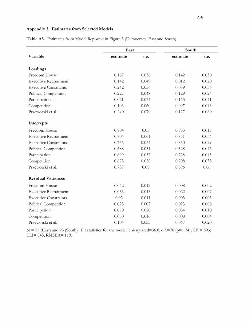
A-8

Appendix 3. Estimates from Selected Models

Table A3. Estimates from Model Reported in Figure 3 (Democracy, East and South)

East South

Variable estimate s.e. estimate s.e.

Loadings Freedom House 0.187 0.056 0.142 0.030 Executive Recruitment 0.142 0.049 0.012 0.020 Executive Constraints 0.242 0.056 0.089 0.036 Political Competition 0.227 0.048 0.129 0.024 Participation 0.021 0.034 0.163 0.041 Competition 0.103 0.060 0.097 0.043 Przeworski et al. 0.240 0.079 0.127 0.060 Intercepts Freedom House 0.804 0.05 0.953 0.019 Executive Recruitment 0.704 0.061 0.851 0.036 Executive Constraints 0.756 0.054 0.850 0.029 Political Competition 0.688 0.031 0.528 0.046 Participation 0.699 0.057 0.728 0.043 Competition 0.673 0.058 0.708 0.035 Przeworski et al. 0.737 0.08 0.896 0.06 Residual Variances Freedom House 0.042 0.013 0.008 0.002 Executive Recruitment 0.035 0.015 0.022 0.007 Executive Constraints 0.02 0.011 0.003 0.003 Political Competition 0.023 0.007 0.023 0.008 Participation 0.070 0.020 0.034 0.010 Competition 0.050 0.016 0.008 0.004 Przeworski et al. 0.104 0.033 0.067 0.020

N = 25 (East) and 23 (South). Fit statistics for the model: chi-squared=36.8, d.f.=26 (p=.124); CFI=.893; TLI=.845; RMSEA=.119.