Embed Size (px)
Citation preview
2 Plant Case Study v9.5dbl_spaced.doc Submitted to the Journal of Manufacturing Systems 06/09/03
1
Evaluating Manufacturing System Design and Performance with the Manufacturing System Design Decomposition Approach David S. Cochran and Daniel C. Dobbs, The Massachusetts Institute of Technology, Cambridge, MA
Abstract
This paper contrasts the design of the manufacturing
systems at two North American automotive component
manufacturing plants with the Manufacturing System
Design Decomposition (MSDD)1. Manufacturing system
designs should not be characterized based on name
alone. Instead of characterizing a manufacturing
system as “mass” or “lean,” it should be described in
terms of the achievement of the manufacturing system
requirements. The following analysis quantifies the
performance of a so-called “lean” plant relative to a so-
called “mass” plant based on the achievement of the
system design requirements decomposed by the
MSDD.
Keywords: Axiomatic Design, Lean
Manufacturing, Manufacturing System Design
1. Introduction
This first objective of the paper is to introduce the
Manufacturing System Design Decomposition
(MSDD). The MSDD is the result of a design
decomposition process to identify clearly the
requirements of a manufacturing system and the means
of achieving those requirements. The ability of a
system design to achieve its requirements can be
evaluated with measurable parameters or measures 2,3.
A “mass” production system is the result of
attempting to optimize the piece-parts or individual
operations within a system. A mass system optimizes
specific parts of a system, instead of the whole. Lean
production is a name given to an enterprise system
design to achieve the requirements of the enterprise as a
whole4,5.
The understanding of what the term “lean” means
can be interpreted in many different ways and has often
led to misinterpretation and misunderstanding. The
purpose of the Manufacturing System Design
Decomposition (MSDD) is to eliminate this ambiguity
by providing a foundation that states clearly the
requirements and means that exist within a system
design. The MSDD applies specifically to the design of
discrete-part, repetitive manufacturing systems. The
requirements are called Functional Requirements (FRs)
and the means are called Design Parameters (DPs)
Revised for Journal of Manufacturing Systems 6/9/2003
2
according to the design methodology used to develop
the Manufacturing System Design Decomposition.
By stating the FRs and DPs of a manufacturing
system design rigorously, the MSDD6,7 provides a
logical foundation to determine whether a
manufacturing system achieves the stated FRs. This
foundation enables the evaluation of existing
manufacturing systems and guides the development of
new manufacturing systems. The MSDD is the result
of applying the Axiomatic Design methodology to
develop a design decomposition to reflect modern
manufacturing requirements.
Definitions proposed in this paper for the terms
“manufacturing system” and “manufacturing system
design” are as follows:
Manufacturing system: The arrangement and operation
of machines, tools, material, people and information to
produce a value-added physical, informational or service
product whose success and cost is characterized by
measurable parameters.
Manufacturing system design: Manufacturing system
design covers all aspects of the creation and operation of
a manufacturing system. Creating the system includes
equipment selection, physical arrangement of equipment,
work design (manual and automatic), and standardization.
The result of the creating process is the factory as it looks
during a shutdown. Operation includes all aspects, which
are necessary to run the created factory (ie., problem
identification and resolution process).
One motivation for developing the MSDD is to
eliminate the ambiguity of defining a system design
with one-word explanations or as a set of physical tools
that are implemented. We assert that it is impossible to
become “lean” simply by implementing “lean tools.”8,9,2
The tools of lean are indicative of a physical means to
achieve certain requirements. These tools encapsulate
the achievement of multiple functional requirements.
In Axiomatic Design, this encapsulation is known as
physical integration.
The decomposition approach first concentrates on
stating the requirement (FR) and then the
corresponding means (DP). Many levels of
decomposition are required before any specific physical
system design becomes apparent. Furthermore, it must
be re-iterated that a lean tool may achieve multiple FRs
simultaneously. This fact is common to Axiomatic
Design which distinguishes physical integration and
functional independence10. A physical entity can
achieve multiple FR and DP pairs and yet be one
physical unit. A problem occurs when a physical tool
is used when the corresponding FR(s) that drove the
original development for that tool no longer exist or are
Revised for Journal of Manufacturing Systems 6/9/2003
3
not understood. The requirements and means must first
be understood before the correct solution can be
designed. The MSDD approach first defines the
manufacturing system requirements (FRs). How the
FRs are accomplished by the means (DPs) is defined
next.
This paper uses a set of performance measures and
the MSDD to evaluate two automotive component-
manufacturing plants located in North America. The
designs of the two plants are evaluated based on the
achievement of the FRs stated by the MSDD and the
performance measures.
One hypothesis or mental model of this research is
that a manufacturing system design that achieves the
requirements (FRs) stated by the MSDD will perform
more cost effectively than a manufacturing system
design that does not effectively achieve the FRs of the
MSDD. This assertion is based on the fact that the
MSDD states an apropos set of FRs relative to modern
manufacturing needs. A key idea is that the concept of
system design as proposed herein requires the
achievement of multiple requirements simultaneously.
The manufacturing “strategy” is, therefore, to achieve
all requirements well and simultaneously.
A second assertion is that to achieve multiple FRs
simultaneously requires a manufacturing system to be
designed. The decomposition process represents the
thinking and the specification of the corresponding
solutions to achieve multiple FRs, simultaneously.
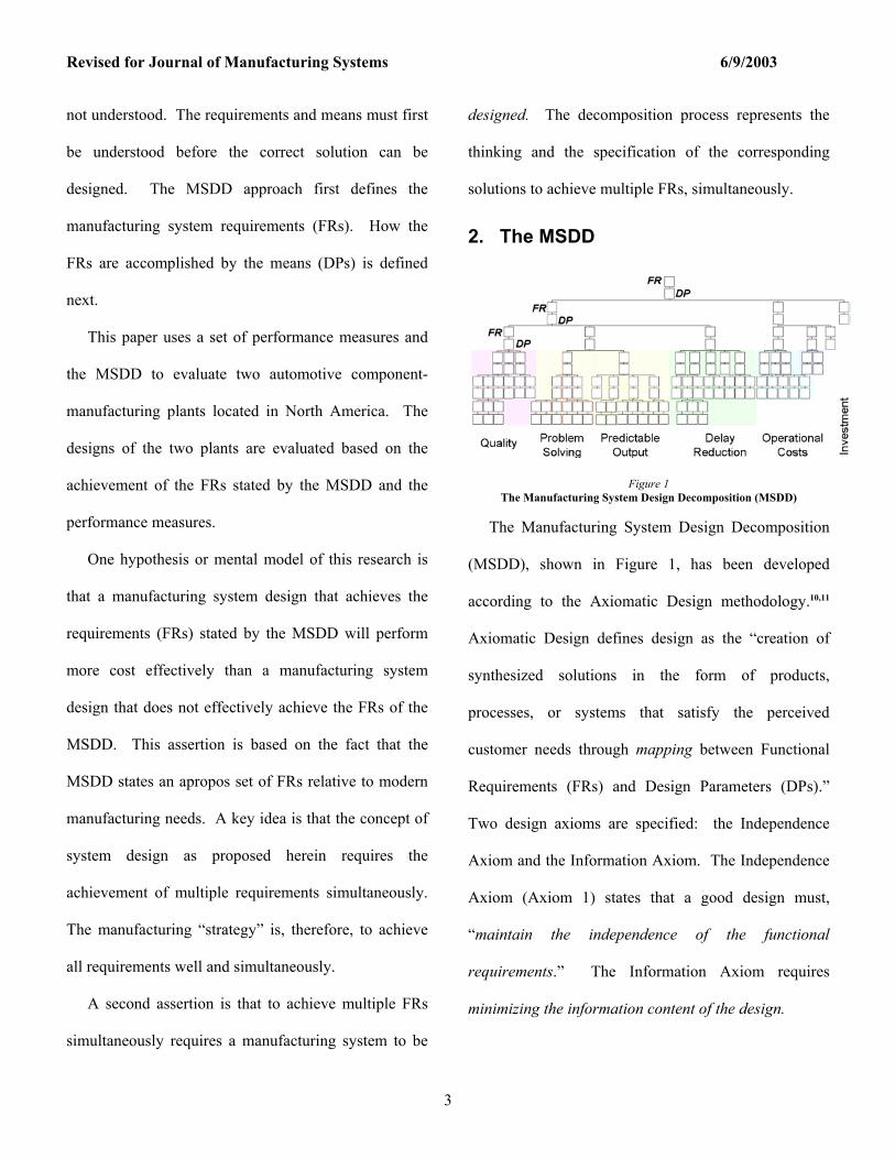
2. The MSDD
Figure 1 The Manufacturing System Design Decomposition (MSDD)
The Manufacturing System Design Decomposition
(MSDD), shown in Figure 1, has been developed
according to the Axiomatic Design methodology.10,11
Axiomatic Design defines design as the “creation of
synthesized solutions in the form of products,
processes, or systems that satisfy the perceived
customer needs through mapping between Functional
Requirements (FRs) and Design Parameters (DPs).”
Two design axioms are specified: the Independence
Axiom and the Information Axiom. The Independence
Axiom (Axiom 1) states that a good design must,
“maintain the independence of the functional
requirements.” The Information Axiom requires
minimizing the information content of the design.
Revised for Journal of Manufacturing Systems 6/9/2003
4
To accomplish independence of the Functional
Requirements requires defining a means, a Design
Parameter (DP), to affect only one Functional
Requirement (FR). Independence also means that the
selection of the DPs ensures that the FRs are
independently satisfied.
2.1 The Design Process
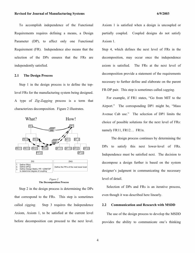
Step 1 in the design process is to define the top-
level FRs for the manufacturing system being designed.
A type of Zig-Zagging process is a term that
characterizes decomposition. Figure 2 illustrates.
FR11 FR12
FR111 FR112 FR121 FR123
ZIG
ZAG
ZIG1. Define FR(s)2. Define DP(s)
Define Design Matrix, FR = [DM]*DPto determine degree of coupling
3.
ZAG
Define the FR’s of the next lower level
FR122
DP11 DP 12
DP 112DP 111
FR1 DP1
DP121 DP123
DP122
What? How!
Figure 2 The Decomposition Process
Step 2 in the design process is determining the DPs
that correspond to the FRs. This step is sometimes
called zigging. Step 3 requires the Independence
Axiom, Axiom 1, to be satisfied at the current level
before decomposition can proceed to the next level.
Axiom 1 is satisfied when a design is uncoupled or
partially coupled. Coupled designs do not satisfy
Axiom 1.
Step 4, which defines the next level of FRs in the
decomposition, may occur once the independence
axiom is satisfied. The FRs at the next level of
decomposition provide a statement of the requirements
necessary to further define and elaborate on the parent
FR-DP pair. This step is sometimes called zagging.
For example, if FR1 states, “Go from MIT to the
Airport.” The corresponding DP1 might be, “Mass
Avenue Cab use.” The selection of DP1 limits the
choice of possible solutions for the next level of FRs:
namely FR11, FR12… FR1n.
The design process continues by determining the
DPs to satisfy this next lower-level of FRs.
Independence must be satisfied next. The decision to
decompose a design further is based on the system
designer’s judgment in communicating the necessary
level of detail.
Selection of DPs and FRs is an iterative process,
even though it was described here linearly.
2.2 Communication and Research with MSDD
The use of the design process to develop the MSDD
provides the ability to communicate one’s thinking
Revised for Journal of Manufacturing Systems 6/9/2003
5
rigorously. If an alternative DP1 were chosen, the next
level of design decomposition could be completely
different. For this reason, this system design approach
fills the huge void that exists today in modern
corporations and institutions: the thinking or thought
process present in many corporations’ designs. The
approach forces one to define one’s thinking. The
result of the decomposition process provides a
structured and adaptable communication tool.
In prior research, Cochran has shown that axiomatic
design may be used to describe the thinking that is
present in mass manufacturing systems5. The authors
define mass production as an incomplete design (fewer
DPs than FRs… which violates axiom 1) and
demonstrate that the unit cost equation used today by
many companies’ drives the physical manufacturing
system design and the behavior within companies.
Many authors have written about the thinking that
creates systems12,13,14. Yet, the problem has been the
inability to effectively communicate one’s thought
process. The system design process with axiomatic
design provides a tool to effectively communicate one’s
thought process. It also forces rigor in ones’ thinking
through the satisfaction of the axioms. Most
importantly, from a research point of view, the MSDD
provides a framework as a type of testable hypothesis,
to prove or to disprove the effectiveness of a system
design.
This study illustrates whether a plant with the so-
called mass plant design performs better than a so-
called lean plant in terms of achieving the FRs of the
MSDD. The FRs define what the system design must
be able to accomplish. Financial measures and unit
cost equations, when used to drive a manufacturing
system design, are too limited in defining what a
system must do.
Optimization of financial measures does not always
result in superior system performance15. For this
reason, this case study seeks to determine whether there
is a relationship between superior achievement of the
FRs and superior performance of the plant as observed
by a set of traditional performance measures.
2.3 Upper Levels of the MSDD
This section describes the thought process in
developing the top two levels of the MSDD. It also
illustrates how to determine if independence has been
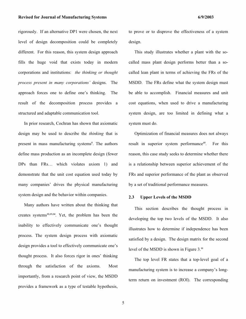
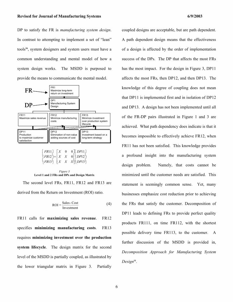
satisfied by a design. The design matrix for the second
level of the MSDD is shown in Figure 3.11
The top level FR states that a top-level goal of a
manufacturing system is to increase a company’s long-
term return on investment (ROI). The corresponding
Revised for Journal of Manufacturing Systems 6/9/2003
6
DP to satisfy the FR is manufacturing system design.
In contrast to attempting to implement a set of “lean”
tools16, system designers and system users must have a
common understanding and mental model of how a
system design works. The MSDD is purposed to
provide the means to communicate the mental model.
DP1Manufacturing System Design
DP11Productionto maximize customersatisfaction
DP12Elimination of non-value adding sources of cost
DP13Investment based on a long-term strategy
FR1Maximize long-term return on investment
FR13Minimize investment over production system lifecycle
FR12Minimize manufacturing costs
FR11Maximize sales revenue
FR
DPDP1Manufacturing System Design
DP11Productionto maximize customersatisfaction
DP12Elimination of non-value adding sources of cost
DP13Investment based on a long-term strategy
FR1Maximize long-term return on investment
FR13Minimize investment over production system lifecycle
FR12Minimize manufacturing costs
FR11Maximize sales revenue
FR
DP
=
131211
000
131211
DPDPDP
XXXXX
X
FRFRFR
Figure 3 Level 1 and 2 FRs and DPs and Design Matrix
The second level FRs, FR11, FR12 and FR13 are
derived from the Return on Investment (ROI) ratio.
ROI = Sales - CostInvestment
(4)
FR11 calls for maximizing sales revenue. FR12
specifies minimizing manufacturing costs. FR13
requires minimizing investment over the production
system lifecycle. The design matrix for the second
level of the MSDD is partially coupled, as illustrated by
the lower triangular matrix in Figure 3. Partially
coupled designs are acceptable, but are path dependent.
A path dependent design means that the effectiveness
of a design is affected by the order of implementation
success of the DPs. The DP that affects the most FRs
has the most impact. For the design in Figure 3, DP11
affects the most FRs, then DP12, and then DP13. The
knowledge of this degree of coupling does not mean
that DP11 is implemented first and in isolation of DP12
and DP13. A design has not been implemented until all
of the FR-DP pairs illustrated in Figure 1 and 3 are
achieved. What path dependency does indicate is that it
becomes impossible to effectively achieve FR12, when
FR11 has not been satisfied. This knowledge provides
a profound insight into the manufacturing system
design problem. Namely, that costs cannot be
minimized until the customer needs are satisfied. This
statement is seemingly common sense. Yet, many
businesses emphasize cost reduction prior to achieving
the FRs that satisfy the customer. Decomposition of
DP11 leads to defining FRs to provide perfect quality
products FR111, on time FR112, with the shortest
possible delivery time FR113, to the customer. A
further discussion of the MSDD is provided in,
Decomposition Approach for Manufacturing System
Design11.
Revised for Journal of Manufacturing Systems 6/9/2003
7
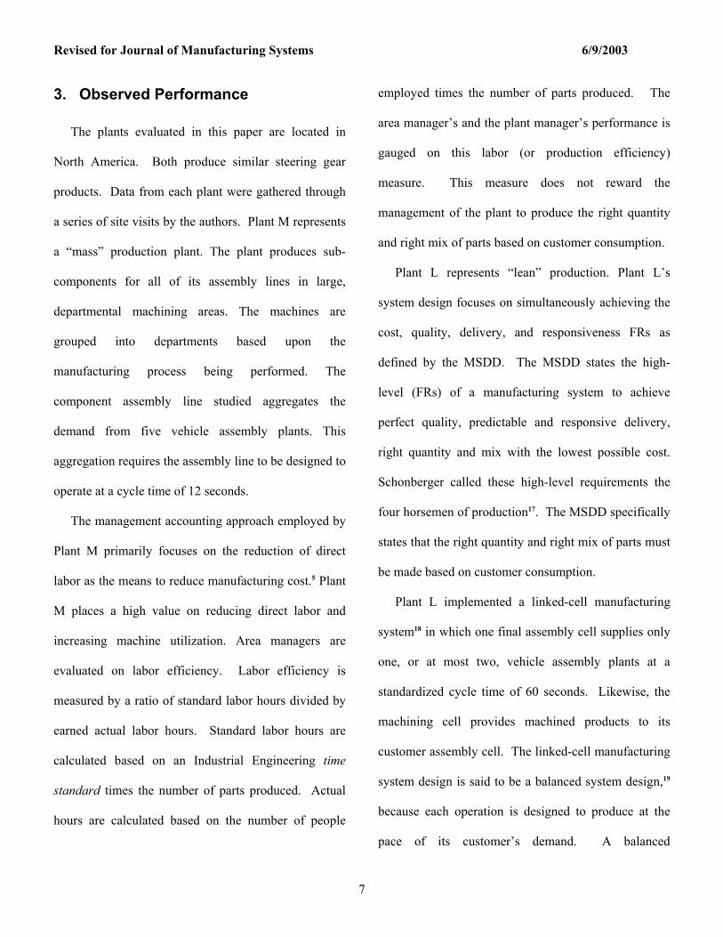
3. Observed Performance
The plants evaluated in this paper are located in
North America. Both produce similar steering gear
products. Data from each plant were gathered through
a series of site visits by the authors. Plant M represents
a “mass” production plant. The plant produces sub-
components for all of its assembly lines in large,
departmental machining areas. The machines are
grouped into departments based upon the
manufacturing process being performed. The
component assembly line studied aggregates the
demand from five vehicle assembly plants. This
aggregation requires the assembly line to be designed to
operate at a cycle time of 12 seconds.
The management accounting approach employed by
Plant M primarily focuses on the reduction of direct
labor as the means to reduce manufacturing cost.5 Plant
M places a high value on reducing direct labor and
increasing machine utilization. Area managers are
evaluated on labor efficiency. Labor efficiency is
measured by a ratio of standard labor hours divided by
earned actual labor hours. Standard labor hours are
calculated based on an Industrial Engineering time
standard times the number of parts produced. Actual
hours are calculated based on the number of people
employed times the number of parts produced. The
area manager’s and the plant manager’s performance is
gauged on this labor (or production efficiency)
measure. This measure does not reward the
management of the plant to produce the right quantity
and right mix of parts based on customer consumption.
Plant L represents “lean” production. Plant L’s
system design focuses on simultaneously achieving the
cost, quality, delivery, and responsiveness FRs as
defined by the MSDD. The MSDD states the high-
level (FRs) of a manufacturing system to achieve
perfect quality, predictable and responsive delivery,
right quantity and mix with the lowest possible cost.
Schonberger called these high-level requirements the
four horsemen of production17. The MSDD specifically
states that the right quantity and right mix of parts must
be made based on customer consumption.
Plant L implemented a linked-cell manufacturing
system18 in which one final assembly cell supplies only
one, or at most two, vehicle assembly plants at a
standardized cycle time of 60 seconds. Likewise, the
machining cell provides machined products to its
customer assembly cell. The linked-cell manufacturing
system design is said to be a balanced system design,19
because each operation is designed to produce at the
pace of its customer’s demand. A balanced
Revised for Journal of Manufacturing Systems 6/9/2003
8
manufacturing system or (value stream) design is
defined as producing at the average pace of customer
demand with the same operating pattern (ie., 2 shifts, 8
hours). A balanced system design produces at the
immediate customer’s takt time.
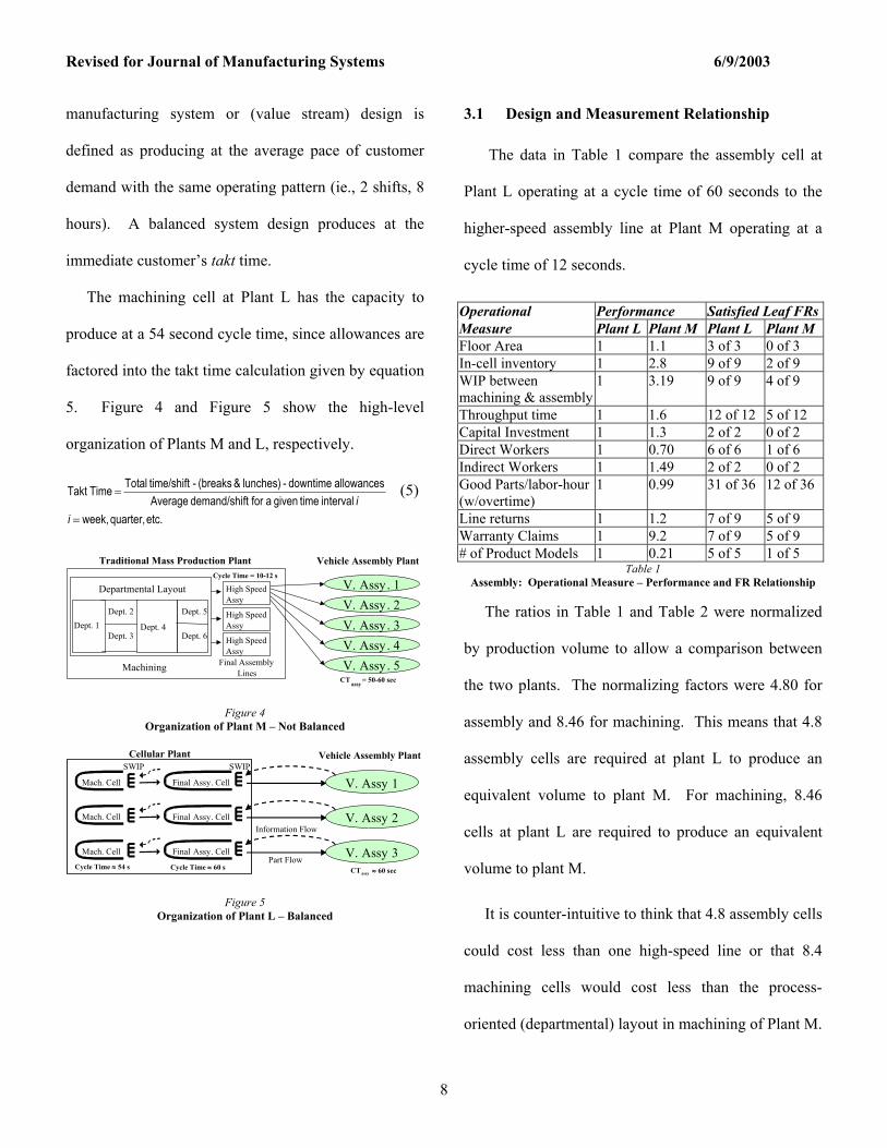
The machining cell at Plant L has the capacity to
produce at a 54 second cycle time, since allowances are
factored into the takt time calculation given by equation
5. Figure 4 and Figure 5 show the high-level
organization of Plants M and L, respectively.
etc. quarter, week, interval time given a forft demand/shi Average
allowances downtime - lunches)& (breaks - time/shift Total TimeTakt
=
=
ii
(5)
High Speed Assy
High Speed Assy
High SpeedAssy
Departmental LayoutCycle Time = 10-12 s
V. Assy. 1V. Assy. 2V. Assy. 3V. Assy. 4V. Assy. 5
CTassy
= 50-60 sec
Traditional Mass Production Plant Vehicle Assembly Plant
Final AssemblyLines
Dept. 3 Dept. 6Dept. 1
Dept. 2 Dept. 5
Dept. 4
Machining
Figure 4 Organization of Plant M – Not Balanced
Cycle Time ≈ 60 s
V. Assy 1
CT assy ≈ 60 secCycle Time ≈ 54 s
V. Assy 2
V. Assy 3Part Flow
Information Flow
Cellular Plant Vehicle Assembly Plant
Final Assy. Cell
Final Assy. Cell
Final Assy. Cell
Mach. Cell
Mach. Cell
Mach. Cell
SWIPSWIP
Figure 5 Organization of Plant L – Balanced
3.1 Design and Measurement Relationship
The data in Table 1 compare the assembly cell at
Plant L operating at a cycle time of 60 seconds to the
higher-speed assembly line at Plant M operating at a
cycle time of 12 seconds.
Table 1 Assembly: Operational Measure – Performance and FR Relationship
The ratios in Table 1 and Table 2 were normalized
by production volume to allow a comparison between
the two plants. The normalizing factors were 4.80 for
assembly and 8.46 for machining. This means that 4.8
assembly cells are required at plant L to produce an
equivalent volume to plant M. For machining, 8.46
cells at plant L are required to produce an equivalent
volume to plant M.
It is counter-intuitive to think that 4.8 assembly cells
could cost less than one high-speed line or that 8.4
machining cells would cost less than the process-
oriented (departmental) layout in machining of Plant M.
Operational Performance Satisfied Leaf FRsMeasure Plant L Plant M Plant L Plant M Floor Area 1 1.1 3 of 3 0 of 3 In-cell inventory 1 2.8 9 of 9 2 of 9 WIP between machining & assembly
1 3.19 9 of 9 4 of 9
Throughput time 1 1.6 12 of 12 5 of 12 Capital Investment 1 1.3 2 of 2 0 of 2 Direct Workers 1 0.70 6 of 6 1 of 6 Indirect Workers 1 1.49 2 of 2 0 of 2 Good Parts/labor-hour (w/overtime)
1 0.99 31 of 36 12 of 36
Line returns 1 1.2 7 of 9 5 of 9 Warranty Claims 1 9.2 7 of 9 5 of 9 # of Product Models 1 0.21 5 of 5 1 of 5
Revised for Journal of Manufacturing Systems 6/9/2003
9
The volume-normalized results in Table 1 indicate
that the assembly line at Plant M has fewer direct
workers in the static, non-operational case. However,
the design at Plant M requires more inventory, has
more work in process (WIP) between machining and
assembly, has a longer throughput time, requires more
investment, produces more defects, has significantly
higher warranty claims, cannot produce as many
product varieties, and requires more indirect workers.
In addition, in actual operation, the number of good
parts per person-hour of operation is equivalent.
According to the investment planning process used by
Plant M (and company M), the cellular approach of
plant L would cost more instead of actually costing
less. The costing approach used by company M uses a
unit cost calculation to drive its investment decisions.
The formula rewards less direct labor. As unit cost is
derived as the sum of direct labor plus material plus
fixed and variable overhead divided by the number of
units produced. Overhead is allocated based on direct
labor time. The less the direct labor content, the less
direct labor time absorption. This emphasis results in
an assembly line design that had less direct labor (.72)
for Plant M vs plant L (1.0) in the non-operational case.
The focus on eliminating wasted motion and work in
Plant L combined with the ability to produce the
customer consumed quantity and mix resulted in
equivalent labor performance during actual operation.
This result shows that optimizing the unit cost equation
did not result in superior performance for Plant M.
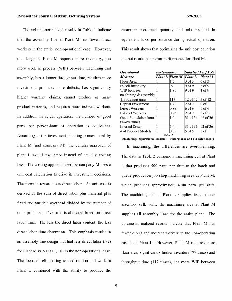
Table 2 Machining: Operational Measure – Performance and FR Relationship
In machining, the differences are overwhelming.
The data in Table 2 compare a machining cell at Plant
L that produces 500 parts per shift to the batch and
queue production job shop machining area at Plant M,
which produces approximately 4200 parts per shift.
The machining cell at Plant L supplies its customer
assembly cell, while the machining area at Plant M
supplies all assembly lines for the entire plant. The
volume-normalized results indicate that Plant M has
fewer direct and indirect workers in the non-operating
case than Plant L. However, Plant M requires more
floor area, significantly higher inventory (97 times) and
throughput time (117 times), has more WIP between
Operational Performance Satisfied Leaf FRsMeasure Plant L Plant M Plant L Plant M Floor Area 1 1.7 3 of 3 0 of 3 In-cell inventory 1 97 9 of 9 2 of 9 WIP between machining & assembly
1 1.81 9 of 9 4 of 9
Throughput time 1 117 12 of 12 5 of 12 Capital Investment 1 1.2 2 of 2 0 of 2 Direct Workers 1 0.86 6 of 6 1 of 6 Indirect Workers 1 0.72 2 of 2 0 of 2 Good Parts/labor-hour (w/overtime)
1 1.0 31 of 36 12 of 36
Internal Scrap 1 5.4 31 of 36 12 of 36 # of Product Models 1 0.35 5 of 5 1 of 5
Revised for Journal of Manufacturing Systems 6/9/2003
10
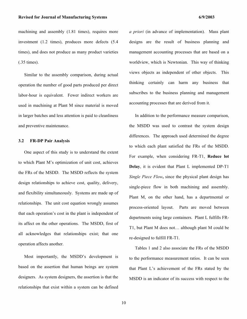
machining and assembly (1.81 times), requires more
investment (1.2 times), produces more defects (5.4
times), and does not produce as many product varieties
(.35 times).
Similar to the assembly comparison, during actual
operation the number of good parts produced per direct
labor-hour is equivalent. Fewer indirect workers are
used in machining at Plant M since material is moved
in larger batches and less attention is paid to cleanliness
and preventive maintenance.
3.2 FR-DP Pair Analysis
One aspect of this study is to understand the extent
to which Plant M’s optimization of unit cost, achieves
the FRs of the MSDD. The MSDD reflects the system
design relationships to achieve cost, quality, delivery,
and flexibility simultaneously. Systems are made up of
relationships. The unit cost equation wrongly assumes
that each operation’s cost in the plant is independent of
its affect on the other operations. The MSDD, first of
all acknowledges that relationships exist; that one
operation affects another.
Most importantly, the MSDD’s development is
based on the assertion that human beings are system
designers. As system designers, the assertion is that the
relationships that exist within a system can be defined
a priori (in advance of implementation). Mass plant
designs are the result of business planning and
management accounting processes that are based on a
worldview, which is Newtonian. This way of thinking
views objects as independent of other objects. This
thinking certainly can harm any business that
subscribes to the business planning and management
accounting processes that are derived from it.
In addition to the performance measure comparison,
the MSDD was used to contrast the system design
differences. The approach used determined the degree
to which each plant satisfied the FRs of the MSDD.
For example, when considering FR-T1, Reduce lot
Delay, it is evident that Plant L implemented DP-T1
Single Piece Flow, since the physical plant design has
single-piece flow in both machining and assembly.
Plant M, on the other hand, has a departmental or
process-oriented layout. Parts are moved between
departments using large containers. Plant L fulfills FR-
T1, but Plant M does not… although plant M could be
re-designed to fulfill FR-T1.
Tables 1 and 2 also associate the FRs of the MSDD
to the performance measurement ratios. It can be seen
that Plant L’s achievement of the FRs stated by the
MSDD is an indicator of its success with respect to the
Revised for Journal of Manufacturing Systems 6/9/2003
11
operational measures. The FRs achieved by Plants L
and M are stated in the Appendix.
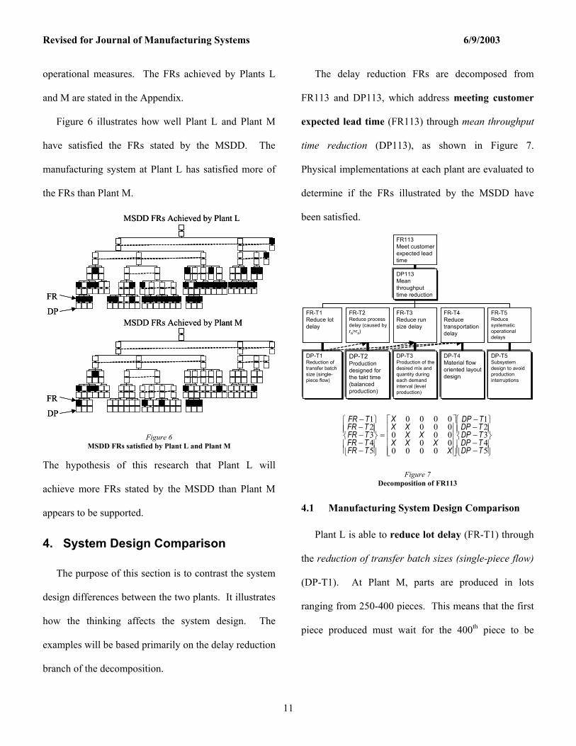
Figure 6 illustrates how well Plant L and Plant M
have satisfied the FRs stated by the MSDD. The
manufacturing system at Plant L has satisfied more of
the FRs than Plant M.
MSDD FRs Achieved by Plant L
MSDD FRs Achieved by Plant M
FR
DP
FR
DP
MSDD FRs Achieved by Plant L
MSDD FRs Achieved by Plant M
FR
DP
FR
DP
Figure 6 MSDD FRs satisfied by Plant L and Plant M
The hypothesis of this research that Plant L will
achieve more FRs stated by the MSDD than Plant M
appears to be supported.
4. System Design Comparison
The purpose of this section is to contrast the system
design differences between the two plants. It illustrates
how the thinking affects the system design. The
examples will be based primarily on the delay reduction
branch of the decomposition.
The delay reduction FRs are decomposed from
FR113 and DP113, which address meeting customer
expected lead time (FR113) through mean throughput
time reduction (DP113), as shown in Figure 7.
Physical implementations at each plant are evaluated to
determine if the FRs illustrated by the MSDD have
been satisfied.
DP113Mean throughput time reduction
DP-T1Reduction of transfer batch size (single-piece flow)
DP-T3Production of the desired mix and quantity during each demand interval (level production)
DP-T5Subsystem design to avoid production interruptions
FR113Meet customer expected lead time
FR-T5Reduce systematic operational delays
FR-T3Reduce run size delay
FR-T1Reduce lot delay
DP-T2Production designed for the takt time(balanced production)
FR-T2Reduce process delay (caused by ra>rs)
DP-T4Material flow oriented layout design
FR-T4Reduce transportation delay
−−−−−
=
−−−−−
54321
0000000000000000
54321
TDPTDPTDPTDPTDP
XXXX
XXXX
X
TFRTFRTFRTFRTFR
Figure 7 Decomposition of FR113
4.1 Manufacturing System Design Comparison
Plant L is able to reduce lot delay (FR-T1) through
the reduction of transfer batch sizes (single-piece flow)
(DP-T1). At Plant M, parts are produced in lots
ranging from 250-400 pieces. This means that the first
piece produced must wait for the 400th piece to be
Revised for Journal of Manufacturing Systems 6/9/2003
12
completed before it can continue to the next station
where it will be processed.
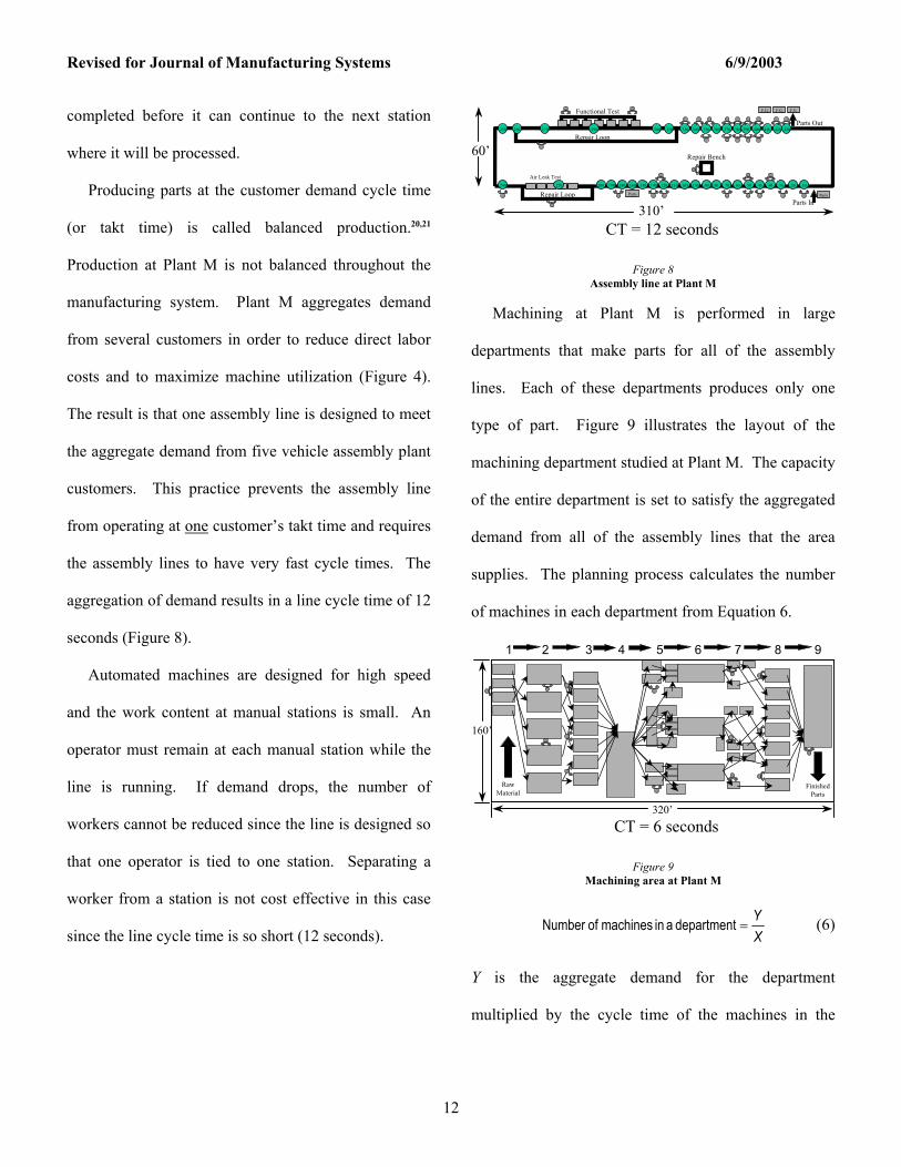
Producing parts at the customer demand cycle time
(or takt time) is called balanced production.20,21
Production at Plant M is not balanced throughout the
manufacturing system. Plant M aggregates demand
from several customers in order to reduce direct labor
costs and to maximize machine utilization (Figure 4).
The result is that one assembly line is designed to meet
the aggregate demand from five vehicle assembly plant
customers. This practice prevents the assembly line
from operating at one customer’s takt time and requires
the assembly lines to have very fast cycle times. The
aggregation of demand results in a line cycle time of 12
seconds (Figure 8).
Automated machines are designed for high speed
and the work content at manual stations is small. An
operator must remain at each manual station while the
line is running. If demand drops, the number of
workers cannot be reduced since the line is designed so
that one operator is tied to one station. Separating a
worker from a station is not cost effective in this case
since the line cycle time is so short (12 seconds).
203050607090120140150160180190
250 370 380 390 400 410 430
110 100 80 40 10
420
240 200
Functional Test
Air Leak Test
Repair Loop
PartsParts
F.G. F.G. F.G.
Repair Loop
Repair Bench
105 45
260 290 320 340 350330 360
Parts In
Parts Out
310’
60’
270
220
300
CT = 12 seconds
Figure 8 Assembly line at Plant M
Machining at Plant M is performed in large
departments that make parts for all of the assembly
lines. Each of these departments produces only one
type of part. Figure 9 illustrates the layout of the
machining department studied at Plant M. The capacity
of the entire department is set to satisfy the aggregated
demand from all of the assembly lines that the area
supplies. The planning process calculates the number
of machines in each department from Equation 6.
1 2 3 4 5 6 7 8 9
RawMaterial
FinishedParts
320’
160’
CT = 6 seconds
Figure 9 Machining area at Plant M
XY
=department a in machines of Number (6)
Y is the aggregate demand for the department
multiplied by the cycle time of the machines in the
Revised for Journal of Manufacturing Systems 6/9/2003
13
department. X is the available operating time for the
department.
The machines in these departments must produce at
high speeds to reduce unit labor cost. This condition
results from the assumption that one person operates
only one or a limited number of machines. Large, high-
speed machines (or processing islands) are designed for
high speed. One person is typically tied to a load
station.
The machining department supplies seven
assembly lines as an aggregate group. The machining
department operates for three shifts, while the assembly
lines operate for one or two shifts. Output from the
machining department must meet the combined
consumption rate of all of the assembly lines. The
average output cycle time is approximately 6 seconds.
DP-T2Production designed for the takt time(balanced production)
DP-T21Definition or grouping of customers to achieve takt times within an ideal range
DP-T22Subsystem enabled to meet the desired takt time (design and operation)
DP-T23Arrival of parts at downstream operations according to pitch
FR-T2Reduce process delay (caused by ra>rs)
FR-T23Ensure that part arrival rate is equal to service rate (ra=rs)
FR-T22Ensure that production cycle time equals takt time
FR-T21Define takt time(s)
−−−
=
−−−
232221
000
232221
TDPTDPTDP
XXXXX
X
TFRTFRTFR
Figure 10 Decomposition of FR-T2
The MSDD illustrates that three FRs must be
satisfied in order to achieve balanced production.
Figure 10 shows the decomposition of FR-T2 and the
corresponding design matrix. Before the assembly and
machining cells at Plant L were built, Plant L defined
the takt times (FR-T21) of the cells by defining [each
cell’s] customers to achieve takt times within an ideal
(cycle time) range (DP-T21). After defining the takt
time, Plant L ensured that the production cycle time
equaled the takt time (FR-T22) with subsystems that
are enabled to meet the desired takt time (DP-T22).
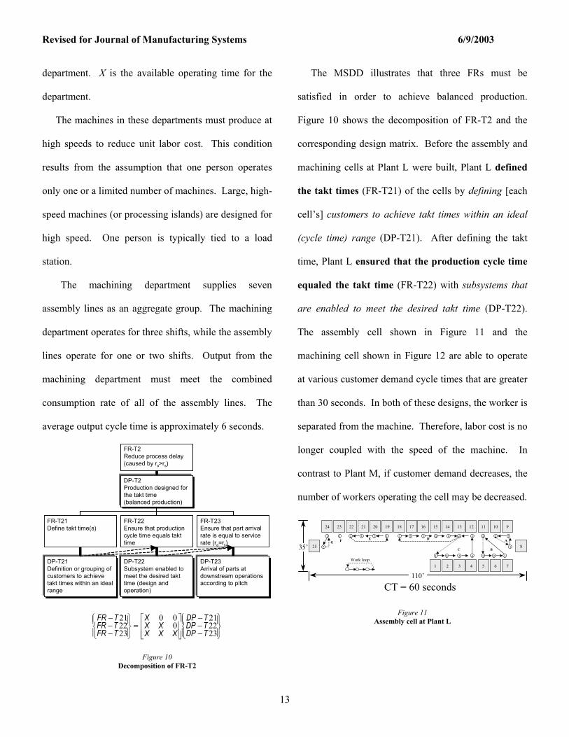
The assembly cell shown in Figure 11 and the
machining cell shown in Figure 12 are able to operate
at various customer demand cycle times that are greater
than 30 seconds. In both of these designs, the worker is
separated from the machine. Therefore, labor cost is no
longer coupled with the speed of the machine. In
contrast to Plant M, if customer demand decreases, the
number of workers operating the cell may be decreased.
25
24 23 22 21 20 19 18 17 16 15 14 13 12 11 10 9
8
1 2 3 4 5 6 7
1 2 3 4
561 2 3 4 5
1 2 3
4
1
234 3 2 111
2
A
BC
DEG F
Work loop
110’
35’
CT = 60 seconds
Figure 11 Assembly cell at Plant L
Revised for Journal of Manufacturing Systems 6/9/2003
14
11
INOUT
1234561
7 8 87 10
234
5 6 9
90’
40’
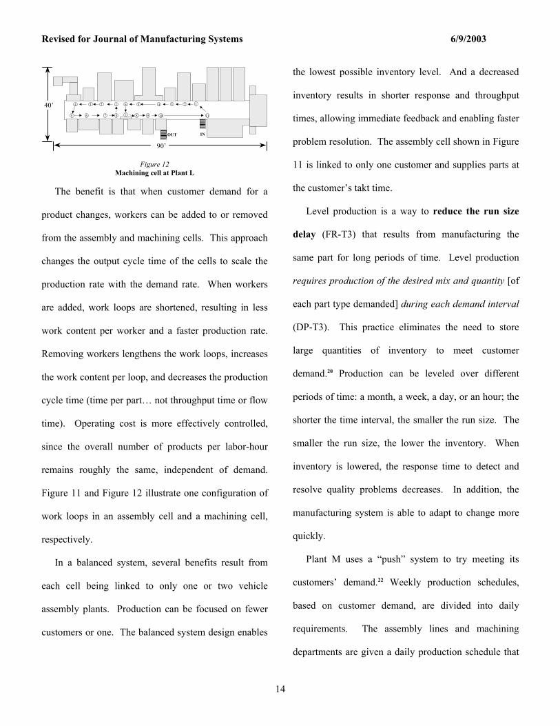
Figure 12 Machining cell at Plant L
The benefit is that when customer demand for a
product changes, workers can be added to or removed
from the assembly and machining cells. This approach
changes the output cycle time of the cells to scale the
production rate with the demand rate. When workers
are added, work loops are shortened, resulting in less
work content per worker and a faster production rate.
Removing workers lengthens the work loops, increases
the work content per loop, and decreases the production
cycle time (time per part… not throughput time or flow
time). Operating cost is more effectively controlled,
since the overall number of products per labor-hour
remains roughly the same, independent of demand.
Figure 11 and Figure 12 illustrate one configuration of
work loops in an assembly cell and a machining cell,
respectively.
In a balanced system, several benefits result from
each cell being linked to only one or two vehicle
assembly plants. Production can be focused on fewer
customers or one. The balanced system design enables
the lowest possible inventory level. And a decreased
inventory results in shorter response and throughput
times, allowing immediate feedback and enabling faster
problem resolution. The assembly cell shown in Figure
11 is linked to only one customer and supplies parts at
the customer’s takt time.
Level production is a way to reduce the run size
delay (FR-T3) that results from manufacturing the
same part for long periods of time. Level production
requires production of the desired mix and quantity [of
each part type demanded] during each demand interval
(DP-T3). This practice eliminates the need to store
large quantities of inventory to meet customer
demand.20 Production can be leveled over different
periods of time: a month, a week, a day, or an hour; the
shorter the time interval, the smaller the run size. The
smaller the run size, the lower the inventory. When
inventory is lowered, the response time to detect and
resolve quality problems decreases. In addition, the
manufacturing system is able to adapt to change more
quickly.
Plant M uses a “push” system to try meeting its
customers’ demand.22 Weekly production schedules,
based on customer demand, are divided into daily
requirements. The assembly lines and machining
departments are given a daily production schedule that
Revised for Journal of Manufacturing Systems 6/9/2003
15
is based on forecast demand from the downstream
customer. When the schedule is not met, the unmade
parts are added to the next day’s schedule.
In the machining departments, production is
scheduled at the input end (e.g. the first set of
operations) of the department. The high level of
inventory, the large number of part-flow combinations,
and the long time intervals between defect creation and
identification all lead to unpredictability in the output.
The assembly lines are often limited to running parts
based upon what parts are available, thus causing
production to deviate further and further from schedule.
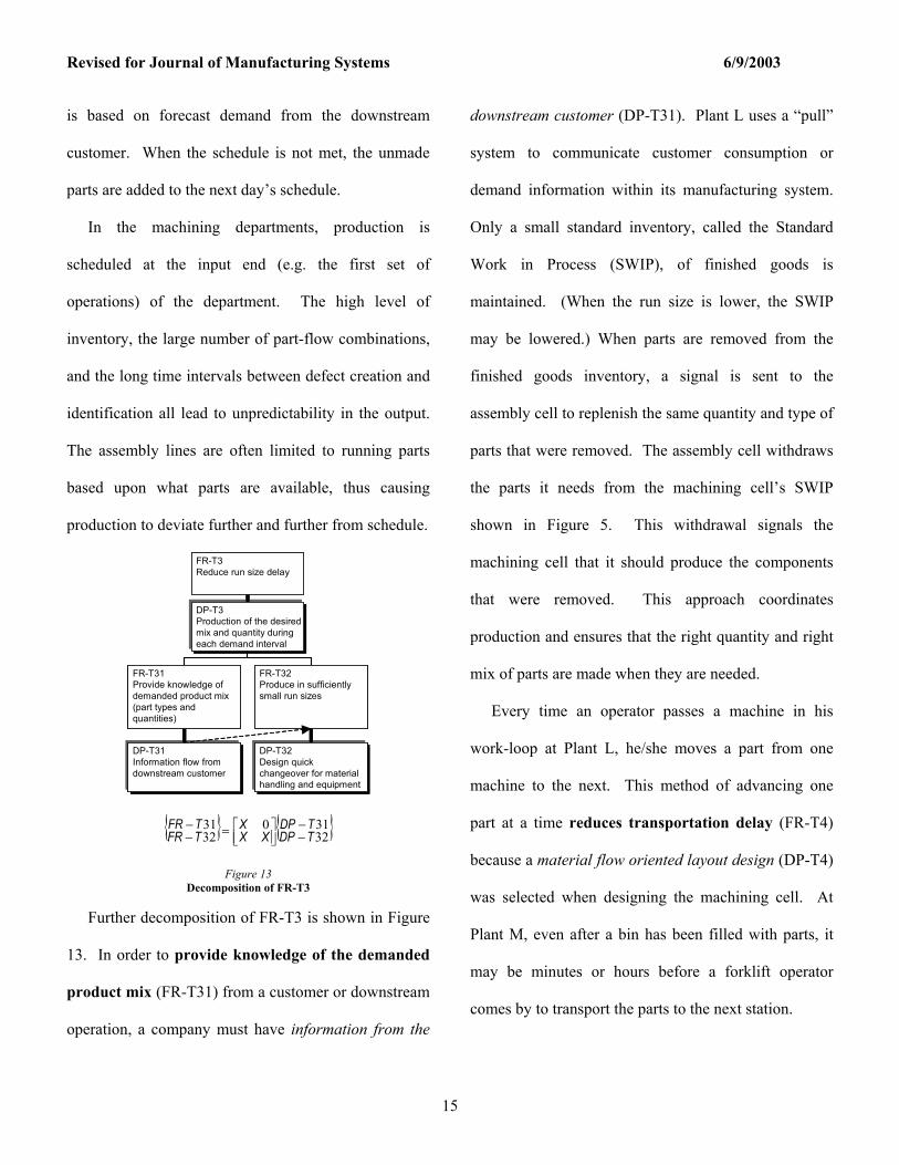
DP-T3Production of the desired mix and quantity during each demand interval
DP-T31Information flow from downstream customer
DP-T32Design quick changeover for material handling and equipment
FR-T3Reduce run size delay
FR-T32Produce in sufficiently small run sizes
FR-T31Provide knowledge of demanded product mix (part types and quantities)
{ } { }32310
3231
TDPTDP
XXX
TFRTFR
−−
=−
−
Figure 13 Decomposition of FR-T3
Further decomposition of FR-T3 is shown in Figure
13. In order to provide knowledge of the demanded
product mix (FR-T31) from a customer or downstream
operation, a company must have information from the
downstream customer (DP-T31). Plant L uses a “pull”
system to communicate customer consumption or
demand information within its manufacturing system.
Only a small standard inventory, called the Standard
Work in Process (SWIP), of finished goods is
maintained. (When the run size is lower, the SWIP
may be lowered.) When parts are removed from the
finished goods inventory, a signal is sent to the
assembly cell to replenish the same quantity and type of
parts that were removed. The assembly cell withdraws
the parts it needs from the machining cell’s SWIP
shown in Figure 5. This withdrawal signals the
machining cell that it should produce the components
that were removed. This approach coordinates
production and ensures that the right quantity and right
mix of parts are made when they are needed.
Every time an operator passes a machine in his
work-loop at Plant L, he/she moves a part from one
machine to the next. This method of advancing one
part at a time reduces transportation delay (FR-T4)
because a material flow oriented layout design (DP-T4)
was selected when designing the machining cell. At
Plant M, even after a bin has been filled with parts, it
may be minutes or hours before a forklift operator
comes by to transport the parts to the next station.
Revised for Journal of Manufacturing Systems 6/9/2003
16
4.2 Equipment Design Comparison
This section of the paper illustrates how machine
design is affected by achieving the FRs of the MSDD.
Machines should not be designed as stand alone
operations, which are isolated from the rest of the
manufacturing system.20
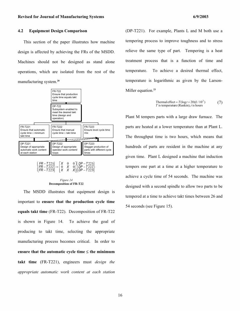
DP-T22Subsystem enabled to meet the desired takt time (design and operation)
DP-T221Design of appropriate automatic work content at each station
DP-T222Design of appropriate operator work content/ loops
DP-T223Stagger production of parts with different cycle times
FR-T22Ensure that production cycle time equals takt time
FR-T223Ensure level cycle time mix
FR-T222Ensure that manual cycle time ≤ takt time
FR-T221Ensure that automatic cycle time ≤ minimum takt time
−−−
=
−−−
223222221
0000
223222221
TDPTDPTDP
XXXX
X
TFRTFRTFR
Figure 14 Decomposition of FR-T22
The MSDD illustrates that equipment design is
important to ensure that the production cycle time
equals takt time (FR-T22). Decomposition of FR-T22
is shown in Figure 14. To achieve the goal of
producing to takt time, selecting the appropriate
manufacturing process becomes critical. In order to
ensure that the automatic cycle time ≤ the minimum
takt time (FR-T221), engineers must design the
appropriate automatic work content at each station
(DP-T221). For example, Plants L and M both use a
tempering process to improve toughness and to stress
relieve the same type of part. Tempering is a heat
treatment process that is a function of time and
temperature. To achieve a desired thermal effect,
temperature is logarithmic as given by the Larson-
Miller equation.23
hours is (Rankin), re temperatuis )10/1)(20(logeffect Thermal 3
tTtT += (7)
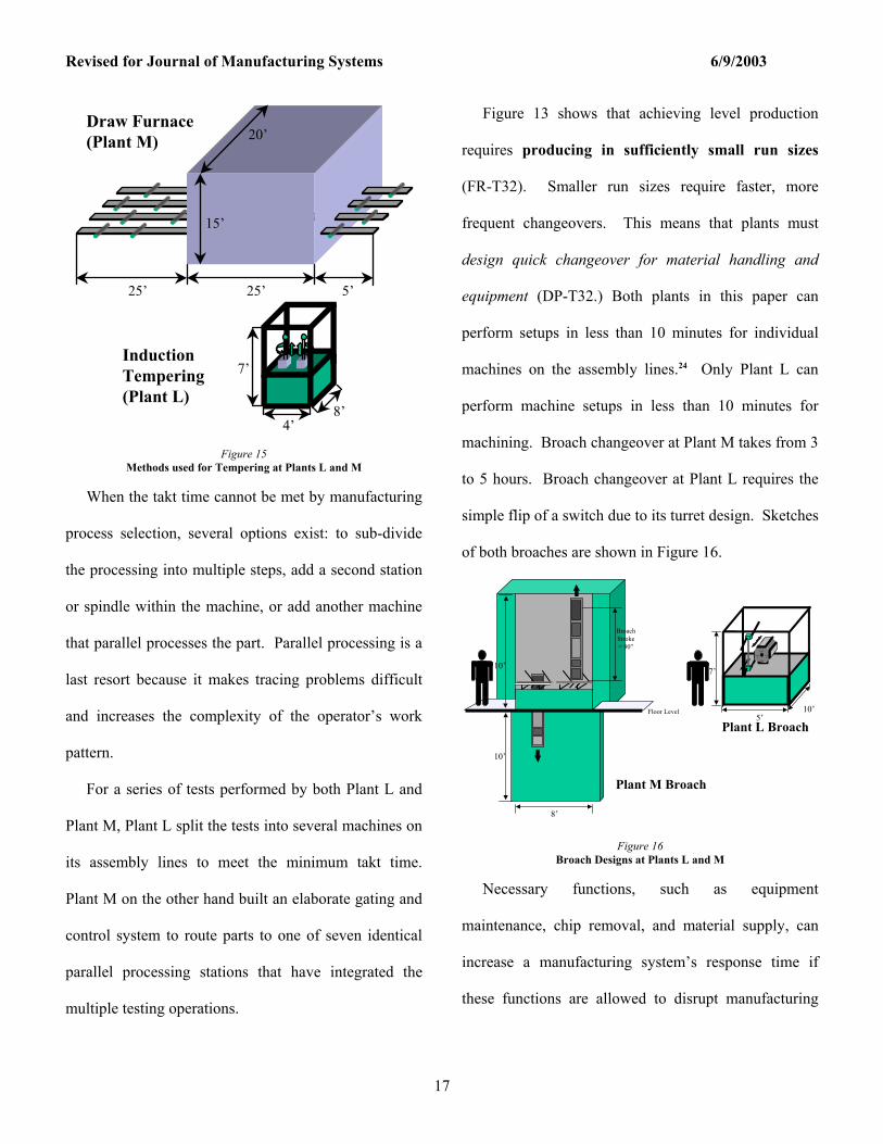
Plant M tempers parts with a large draw furnace. The
parts are heated at a lower temperature than at Plant L.
The throughput time is two hours, which means that
hundreds of parts are resident in the machine at any
given time. Plant L designed a machine that induction
tempers one part at a time at a higher temperature to
achieve a cycle time of 54 seconds. The machine was
designed with a second spindle to allow two parts to be
tempered at a time to achieve takt times between 26 and
54 seconds (see Figure 15).
Revised for Journal of Manufacturing Systems 6/9/2003
17
25’ 25’ 5’
15’
20’Draw Furnace(Plant M)
7’
8’4’
InductionTempering(Plant L)
Figure 15 Methods used for Tempering at Plants L and M
When the takt time cannot be met by manufacturing
process selection, several options exist: to sub-divide
the processing into multiple steps, add a second station
or spindle within the machine, or add another machine
that parallel processes the part. Parallel processing is a
last resort because it makes tracing problems difficult
and increases the complexity of the operator’s work
pattern.
For a series of tests performed by both Plant L and
Plant M, Plant L split the tests into several machines on
its assembly lines to meet the minimum takt time.
Plant M on the other hand built an elaborate gating and
control system to route parts to one of seven identical
parallel processing stations that have integrated the
multiple testing operations.
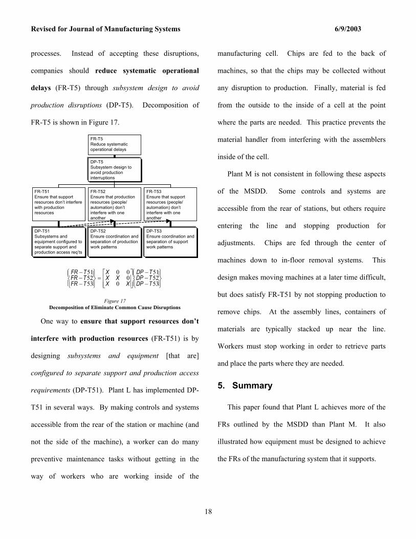
Figure 13 shows that achieving level production
requires producing in sufficiently small run sizes
(FR-T32). Smaller run sizes require faster, more
frequent changeovers. This means that plants must
design quick changeover for material handling and
equipment (DP-T32.) Both plants in this paper can
perform setups in less than 10 minutes for individual
machines on the assembly lines.24 Only Plant L can
perform machine setups in less than 10 minutes for
machining. Broach changeover at Plant M takes from 3
to 5 hours. Broach changeover at Plant L requires the
simple flip of a switch due to its turret design. Sketches
of both broaches are shown in Figure 16.
10’
10’
8’
BroachStroke= 90”
Floor Level
Plant M Broach
FinishB
RoughB
FinishA
RoughA
7’
5’10’
Plant L Broach
Figure 16 Broach Designs at Plants L and M
Necessary functions, such as equipment
maintenance, chip removal, and material supply, can
increase a manufacturing system’s response time if
these functions are allowed to disrupt manufacturing
Revised for Journal of Manufacturing Systems 6/9/2003
18
processes. Instead of accepting these disruptions,
companies should reduce systematic operational
delays (FR-T5) through subsystem design to avoid
production disruptions (DP-T5). Decomposition of
FR-T5 is shown in Figure 17.
DP-T5Subsystem design to avoid production interruptions
DP-T51Subsystems and equipment configured to separate support and production access req’ts
DP-T52Ensure coordination and separation of production work patterns
DP-T53Ensure coordination and separation of support work patterns
FR-T5Reduce systematic operational delays
FR-T53Ensure that support resources (people/ automation) don’t interfere with one another
FR-T52Ensure that production resources (people/ automation) don’t interfere with one another
FR-T51Ensure that support resources don’t interfere with production resources
−−−
=
−−−
535251
0000
535251
TDPTDPTDP
XXXX
X
TFRTFRTFR
Figure 17 Decomposition of Eliminate Common Cause Disruptions
One way to ensure that support resources don’t
interfere with production resources (FR-T51) is by
designing subsystems and equipment [that are]
configured to separate support and production access
requirements (DP-T51). Plant L has implemented DP-
T51 in several ways. By making controls and systems
accessible from the rear of the station or machine (and
not the side of the machine), a worker can do many
preventive maintenance tasks without getting in the
way of workers who are working inside of the
manufacturing cell. Chips are fed to the back of
machines, so that the chips may be collected without
any disruption to production. Finally, material is fed
from the outside to the inside of a cell at the point
where the parts are needed. This practice prevents the
material handler from interfering with the assemblers
inside of the cell.
Plant M is not consistent in following these aspects
of the MSDD. Some controls and systems are
accessible from the rear of stations, but others require
entering the line and stopping production for
adjustments. Chips are fed through the center of
machines down to in-floor removal systems. This
design makes moving machines at a later time difficult,
but does satisfy FR-T51 by not stopping production to
remove chips. At the assembly lines, containers of
materials are typically stacked up near the line.
Workers must stop working in order to retrieve parts
and place the parts where they are needed.
5. Summary
This paper found that Plant L achieves more of the
FRs outlined by the MSDD than Plant M. It also
illustrated how equipment must be designed to achieve
the FRs of the manufacturing system that it supports.
Revised for Journal of Manufacturing Systems 6/9/2003
19
On average, Plant L satisfied 96% of the FRs while
Plant M only satisfied 23%. Plant M was developed to
optimize the unit cost equation, which is focused on
optimizing the cost of individual operations in the
plant. The business planning process and the
management accounting process used by Plant M are
derived from this thinking. This viewpoint assumes
that minimizing the sum of the individual operating
costs reduces total cost.
The Manufacturing System Design Decomposition
(MSDD) illustrates that the system design used by Plant
L performs better than Plant M in a side-by-side
comparison. This result challenges the assumption that
lower cost is the result of optimizing the sum of the
individual operation costs. In addition, the linked-
cellular manufacturing system can accommodate
volumes as high as the “mass” plant, by simply
replicating the linked-cell value streams.
The MSDD allows system designers to see and
understand the interrelationships that exist in
manufacturing systems. Plant L’s superior operational
performance and achievement of most of the FRs stated
by the MSDD, suggests that a design decomposition
approach may be used to design plants with superior
performance. This finding provides additional
understanding that a science base for system design can
be truly realized, which was Suh’s original statement of
the need for developing axiomatic design.
Plant M illustrates the problems that occur when
sub-elements are optimized independently of the whole.
The MSDD provides a framework for understanding
the requirements and means that are necessary to design
effective manufacturing systems. It forms the basis for
designing, controlling, and communicating the web of
interrelationships that exist in any manufacturing
system, without the use of buzzwords and
superficiality.
References
1. B.J. Carrus, D.S. Cochran, Application of a Design Methodology
for Production Systems, Proceedings of the 2nd International
Conference on Engineering Design and Automation, Maui, Hawaii,
August 9-12, 1998.
2. N.P. Suh, D.S. Cochran, and P.C. Lima, 1998, Manufacturing
System Design, Annals of 48th General Assembly of CIRP, Vol.
47/2/1998, pp. 627-639.
3. A. DeToni, G. Nassimbeni, S. Tonchia, “Integrated Production
Performance Measurement System,” Industrial Management and
Data Systems, Vol 5, No. 6, 1997, pp. 180-186.
4. H.T. Johnson, Relevance Regained, (New York, NY: Simon &
Schuster, 1992).
5. D.S. Cochran, Y.S. Kim, J. Kim “The Alignment of Performance
Measurement with the Manufacturing System Design,” First
International Conference on Axiomatic Design, (Cambridge, MA:
June 21-23, 2000).
Revised for Journal of Manufacturing Systems 6/9/2003
20
6 D.S. Cochran, “The Production System Design and Deployment
Framework," IAM/SAE (Detroit, MI: May 11-13, 1999) paper
#1999-01-1644.
7. D.S. Cochran, P.C. Lima, “Lean Production System Design
Decomposition Version 4.2,” internal working document of the
Production System Design Laboratory (Cambridge, MA: MIT
1998).
8. W.J. Hopp, M.L Spearman, Factory Physics (Boston, MA:
Irwin/McGraw-Hill, 1996), pp 55-63.
9. J.P. Womack, D.T. Jones, Lean Thinking (New York, NY: Simon
& Schuster, 1996).
10. N.P. Suh, The Principles of Design (New York: Oxford
University Press, 1990).
11. D.S. Cochran, J.F. Arinez, J.W. Duda, J. Linck, “A
Decomposition Approach for Manufacturing System Design,”
submitted to Journal of Manufacturing Systems, September 2000.
12. M. J. Wheatley, Leadership and the New Science: Discovering
Order in a Chaotic World, 2nd Edition (Berrett-Koehler Publishers:
San Francisco, 1999).
13. H. T. Johnson and A. Broms, Profit Beyond Measure:
Extraordinary Results through Attention to Work and People, (New
York, NY: The Free Press, 2000).
14. S. Spear and H. Bowen, “Decoding the DNA of the Toyota
Production System,” HBR, September-October, 1999, pp 96-106.
15. B. Maskell, Performance Measurement for World Class
Manufacturing: A Model for American Companies, (Portland, OR:
Productivity Press, 1994).
16. R.H. Hayes, G.P. Pisano, “Beyond World-Class: The New
Manufacturing Strategy,” Harvard Business Review.
January/February 1994, pp.77-86.
17. R.J. Schonberger, World Class Manufacturing: The Lessons of
Simplicity Applied, (Macmillan, NY: The Free Press, 1986.)
18. JT. Black, The Design of the Factory With a Future, (New
York: McGraw-Hill, 1991).
19. Y. Monden, Toyota Production System (Norcross, GA: IIE
Press, 1983).
20. S. Shingo, A Study of the Toyota Production System from an
Industrial Engineering Point of View (Cambridge: Productivity
Press, 1989).
21. T. Ohno, Toyota Production System (Portland, OR: Productivity
Press, 1988).
22. U. Karmakar, “Getting Control of Just-in-Time,” Harvard
Business Review. September/October 1989, pp.122-131.
23. D.A. Canonico, Metals Handbook, Vol. 9, (Metals Park, OH:
American Society for Metals, 1978).
24. S. Shingo, A Revolution in Manufacturing: The SMED System,
(Portland, OR: Productivity Press, 1985).
Biographies
Prof. David Cochran is an Associate Professor of Mechanical
Engineering at MIT. He founded the Production System Design
Laboratory, an initiative within the Laboratory for Manufacturing
and Productivity, to develop a comprehensive approach for the
design and implementation of production systems. He is a recipient
of the “Shingo Prize for Manufacturing Excellence.” He has taught
over 30 manufacturers the implementation and underlying
principles of production system design. Dr. Cochran serves on the
Board of Directors of the Greater Boston Manufacturing Partnership
and the AMA. Prior to joining MIT, Dr. Cochran worked with Ford
Motor Company. He holds a Ph.D. and B.S. degrees from Auburn
University, and a M.S. degree from the Pennsylvania State
Revised for Journal of Manufacturing Systems 6/9/2003
21
University. He is a member of the AME, IIE, SME, APICS, and
ASME.
Daniel Dobbs recently completed dual master’s degrees in the
Mechanical Engineering department and the Technology and Policy
Program at the Massachusetts Institute of Technology. His research
focused on the design and development of new manufacturing
systems in existing industries. He is now working as a
manufacturing engineer at Texas Instruments in Attleboro, MA.
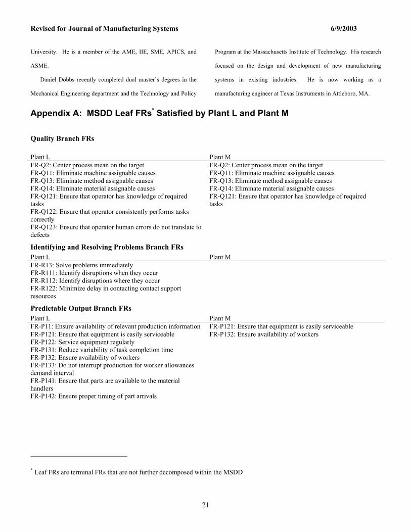
Appendix A: MSDD Leaf FRs* Satisfied by Plant L and Plant M
Quality Branch FRs
Plant L Plant M FR-Q2: Center process mean on the target FR-Q2: Center process mean on the target FR-Q11: Eliminate machine assignable causes FR-Q11: Eliminate machine assignable causes FR-Q13: Eliminate method assignable causes FR-Q13: Eliminate method assignable causes FR-Q14: Eliminate material assignable causes FR-Q14: Eliminate material assignable causes FR-Q121: Ensure that operator has knowledge of required tasks
FR-Q121: Ensure that operator has knowledge of required tasks
FR-Q122: Ensure that operator consistently performs tasks correctly
FR-Q123: Ensure that operator human errors do not translate to defects
Identifying and Resolving Problems Branch FRs Plant L Plant M FR-R13: Solve problems immediately FR-R111: Identify disruptions when they occur FR-R112: Identify disruptions where they occur FR-R122: Minimize delay in contacting contact support resources
Predictable Output Branch FRs Plant L Plant M FR-P11: Ensure availability of relevant production information FR-P121: Ensure that equipment is easily serviceable FR-P121: Ensure that equipment is easily serviceable FR-P132: Ensure availability of workers FR-P122: Service equipment regularly FR-P131: Reduce variability of task completion time FR-P132: Ensure availability of workers FR-P133: Do not interrupt production for worker allowances demand interval
FR-P141: Ensure that parts are available to the material handlers
FR-P142: Ensure proper timing of part arrivals
* Leaf FRs are terminal FRs that are not further decomposed within the MSDD
Revised for Journal of Manufacturing Systems 6/9/2003
22
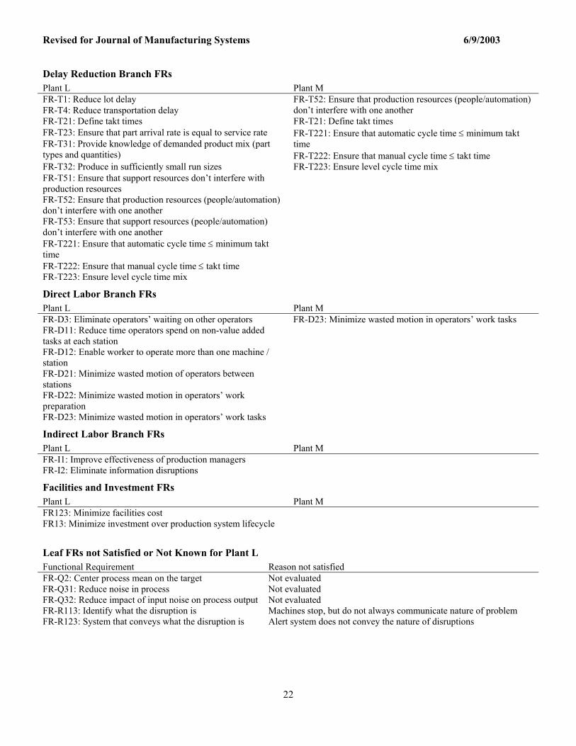
Delay Reduction Branch FRs Plant L Plant M FR-T1: Reduce lot delay FR-T4: Reduce transportation delay
FR-T52: Ensure that production resources (people/automation) don’t interfere with one another
FR-T21: Define takt times FR-T21: Define takt times FR-T23: Ensure that part arrival rate is equal to service rate FR-T221: Ensure that automatic cycle time ≤ minimum takt
time FR-T31: Provide knowledge of demanded product mix (part types and quantities) FR-T222: Ensure that manual cycle time ≤ takt time FR-T32: Produce in sufficiently small run sizes FR-T223: Ensure level cycle time mix FR-T51: Ensure that support resources don’t interfere with production resources
FR-T52: Ensure that production resources (people/automation) don’t interfere with one another
FR-T53: Ensure that support resources (people/automation) don’t interfere with one another
FR-T221: Ensure that automatic cycle time ≤ minimum takt time
FR-T222: Ensure that manual cycle time ≤ takt time FR-T223: Ensure level cycle time mix
Direct Labor Branch FRs Plant L Plant M FR-D3: Eliminate operators’ waiting on other operators FR-D23: Minimize wasted motion in operators’ work tasks FR-D11: Reduce time operators spend on non-value added tasks at each station
FR-D12: Enable worker to operate more than one machine / station
FR-D21: Minimize wasted motion of operators between stations
FR-D22: Minimize wasted motion in operators’ work preparation
FR-D23: Minimize wasted motion in operators’ work tasks
Indirect Labor Branch FRs Plant L Plant M FR-I1: Improve effectiveness of production managers FR-I2: Eliminate information disruptions
Facilities and Investment FRs Plant L Plant M FR123: Minimize facilities cost FR13: Minimize investment over production system lifecycle
Leaf FRs not Satisfied or Not Known for Plant L Functional Requirement Reason not satisfied FR-Q2: Center process mean on the target Not evaluated FR-Q31: Reduce noise in process Not evaluated FR-Q32: Reduce impact of input noise on process output Not evaluated FR-R113: Identify what the disruption is Machines stop, but do not always communicate nature of problem FR-R123: System that conveys what the disruption is Alert system does not convey the nature of disruptions
Revised for Journal of Manufacturing Systems 6/9/2003
23
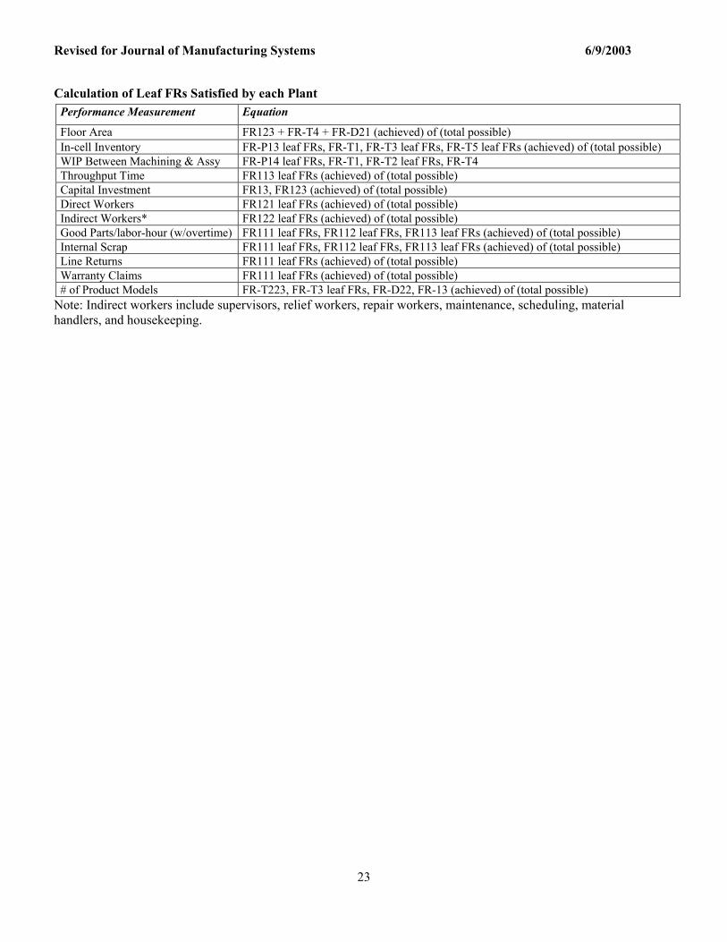
Calculation of Leaf FRs Satisfied by each Plant Performance Measurement Equation
Floor Area FR123 + FR-T4 + FR-D21 (achieved) of (total possible) In-cell Inventory FR-P13 leaf FRs, FR-T1, FR-T3 leaf FRs, FR-T5 leaf FRs (achieved) of (total possible) WIP Between Machining & Assy FR-P14 leaf FRs, FR-T1, FR-T2 leaf FRs, FR-T4 Throughput Time FR113 leaf FRs (achieved) of (total possible) Capital Investment FR13, FR123 (achieved) of (total possible) Direct Workers FR121 leaf FRs (achieved) of (total possible) Indirect Workers* FR122 leaf FRs (achieved) of (total possible) Good Parts/labor-hour (w/overtime) FR111 leaf FRs, FR112 leaf FRs, FR113 leaf FRs (achieved) of (total possible) Internal Scrap FR111 leaf FRs, FR112 leaf FRs, FR113 leaf FRs (achieved) of (total possible) Line Returns FR111 leaf FRs (achieved) of (total possible) Warranty Claims FR111 leaf FRs (achieved) of (total possible) # of Product Models FR-T223, FR-T3 leaf FRs, FR-D22, FR-13 (achieved) of (total possible)
Note: Indirect workers include supervisors, relief workers, repair workers, maintenance, scheduling, material handlers, and housekeeping.