Embed Size (px)
Citation preview
1
Evaluating Opportunities for Increasing Power
Capacity of Existing Overhead Line Systems
K. Kopsidas and S. M. Rowland
The University of Manchester
School of Electrical and Electronic Engineering,
PO Box 88, Manchester, M60 1QD, UK.
Keywords: AAAC, ACSR, ampacity, composite conductors, conductor creep, high
temperature, overhead line, re-conductoring, re-tensioning, sag, wood pole structure.
Abstract
Re-tensioning and/or re-conductoring are considered the most popular cost-effective
ways to increase the efficiency of power capacity of an existing aerial line. The
identification of the most beneficial method requires ampacity and sag calculations to
consider all the system factors that influence its performance. A holistic methodology for
calculating conductor ampacity and sag at any temperature and power frequency when
different conductors are implemented onto a pre-specified overhead line structure is used
to illustrate how the properties of the conductors allow opportunities for thermal and
voltage uprating on existing Overhead Line Systems. This is achieved through a
comparative analysis of the electrical and mechanical behaviour of conductors of
different technologies and sizes on a 33 kV wood pole system. The analysis focuses on
normal operating temperatures for novel conductors which can operate at elevated
temperatures to avoid the increase in losses, and also allow the comparison with
conventional conductors in order to identify potential benefits for the investigated OHL
system.

2
1. Introduction
The need to increase the power transfer capacity of existing overhead lines (OHL) by
cost-effective and environmentally-friendly methods within a competitive deregulated
market is directly linked with an increase in the associated conductors’ ampacity (i.e.
current capacity). Two of the most popular ways that can be employed to achieve this are
re-tensioning and re-conductoring. The former is based on maximising the conductor’s
clearance to the ground by increasing its tension, allowing an increase in operating
conductor thermal expansion facilitating higher current flows. Re-tensioning is usually
applied in old lines for which the conductor sag is the limiting factor for increasing a
line’s thermal rating or on surveyed lines which experienced severe weather and
electrical loading out of the predicted design conditions. Error in sag prediction may
result in the need for line re-tensioning. This error is a common consequence of the
misinterpretation of the conversion of conductor plastic elongation to thermal elongation,
based on experimental data or standards [1].
Alternatively, re-conductoring involves replacing the existing conductors with conductors
of larger sizes or alternative materials and technologies. Several new conductors have
been designed and produced to yield an increase in power transfer capability. These
technologies mainly attempt to increase the conductor’s performance by increasing its
maximum (continuous) operating temperature, therefore increasing its maximum current
capacity. Moreover, recent composite designs like ‘aluminium conductor composite
reinforced’ (ACCR) and ‘aluminium conductor composite core’ (ACCC) [2-3] are
independent of steel’s weight and coefficient of thermal expansion. This independence
3
may be the key to these conductors’ improved performance at both normal as well as
elevated operating temperatures. Such conductors are commonly called high temperature
low sag (HTLS) conductors.
The implementation of changes required for uprating an existing line are related to the
cost, time and outages needed. The thermal uprating of existing OHL by re-tensioning or
re-conductoring is advantageous as it requires fewer modifications and less
implementation time than other methods [4]. In contrast, voltage level upgrading involves
more changes and takes more time to implement particularly when additional rights-of-
way are required usually resulting in higher costs [5-6].
It should be emphasised that the existing literature [3-4, 7-9] evaluates the performance
of different HTLS conductors by direct comparison with aluminium conductor steel
reinforced (ACSR), as most HTLS conductors have a steel core as strength member, and
not with the lighter and more conductive all aluminium alloy conductor (AAAC) type.
Furthermore, limited work has been done to examine conductor performance with a
realistic power line structure to evaluate the real benefits of HTLS conductors when
compared with ACSRs and AAACs. No evaluation of the improved performance
conductors on aerial wood pole lines has been presented, apart from our recent analysis
[10]. In that work we reported the improvement offered by re-conductoring in the power
transfer capacity of a 33kV wood pole structure. The focus was mainly on the
comparison of the mechanical and electrical performance of AAAC and ACSR
conductors. To aid this comparison, a ‘three sag zones’ theory was proposed. In this
4
paper we build and extend this theory by identifying the critical properties of the
conductors and their materials and the way these are affecting the zones. To do so we use
a case study of a similar structure but different in respect to the limitations it poses to the
system performance in order to extend the results, adding also more standard (American)
conductor sizes. Furthermore, comparison of similar weight conductors is performed as
this property is more critical for weak wood poles. In addition, analysis is performed for
sag at different temperatures and different span lengths.
Hence, this paper focuses on conductors’ properties that could allow opportunities for
increasing the power capacity of an existing 33 kV wood pole OHL system. Such
properties include the coefficient of thermal expansion, elasticity, strength and weight. In
addition, analysis considers the effect of the increase in operating temperature on the
ampacity, losses, and sag. This analysis is performed using the methodology described in
the following section.
2. Methodology: A Holistic Perspective on Ampacity and Sag Computations
The conductor’s maximum current capacity limits the maximum power transfer
capability of the OHL system. This current is usually referred to as ampacity and is
limited by properties relevant to conductor design, the surrounding environment,
operational conditions and the OHL structure design (as this defines the conductor size).
These properties influence the elastic, plastic and thermal elongation which are
proportional to conductor weight, tension, and current flow, respectively, and thus result
in altering conductor sag. Sag defines the height difference between two points of the
5
conductor: one located at the suspension fittings and the other located at mid-span. Sag,
therefore, defines the system’s minimum ground clearance. There are two critical sag
conditions considered during the design of an OHL system which define the maximum
total (i.e. considering elastic, plastic and thermal) conductor elongation:
1. The maximum mechanical loading occurs at the designed maximum weather
loading of the system (i.e. when ice is attached or wind is battering the
conductor). This condition also yields the maximum conductor tension (MCT).
2. The maximum electrical loading, occurs when the tension is at the minimum
because of the thermal elongation caused by the current flow. Usually, during
these electrical loading conditions, the most severe sag and minimum ground
clearance, limit any further increase in current flow. This current flow is affected
by the ambient conditions, hence seasonal ampacities become common practice;
these seasonal ampacities are defined by the average ambient conditions and
maximum operating conductor temperature (TMAX).
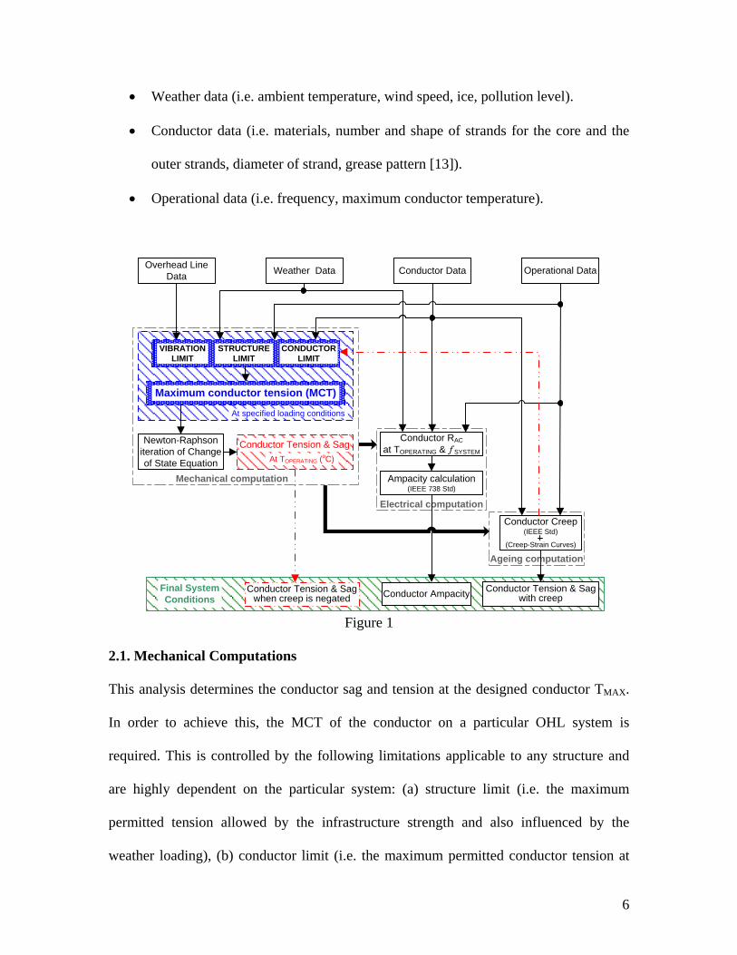
The methodology which is briefly outlined here for the readers’ convenience is detailed
in [11-12]. The process is illustrated in the flowchart of Fig. 1 and emphasises the key
electromechanical elements influencing conductor sag and ampacity calculations. The
computations involved in this process are divided into three different steps which are
performed separately and then linked together to compute the final conditions. Therefore,
a holistic perspective on the system performance is taken by considering four different
data groups for the calculations:
Overhead line data of support structure (i.e. structure type and dimensions, tensile
loading strength, weight strength, latitude, azimuth and elevation).
6
Weather data (i.e. ambient temperature, wind speed, ice, pollution level).
Conductor data (i.e. materials, number and shape of strands for the core and the
outer strands, diameter of strand, grease pattern [13]).
Operational data (i.e. frequency, maximum conductor temperature).
Electrical computation
Ageing computation
Overhead Line
DataOperational Data
Newton-Raphson
iteration of Change
of State Equation
Conductor Tension & Sag
Conductor Ampacity
Conductor RAC
at TOPERATING & ƒSYSTEM
Weather Data Conductor Data
Conductor Creep (IEEE Std)
(Creep-Strain Curves)
Final System
Conditions
Ampacity calculation(IEEE 738 Std)
Conductor Tension & Sag with creep
Maximum conductor tension (MCT)
Conductor Tension & Sag when creep is negated
Mechanical computation
At specified loading conditions
VIBRATION
LIMIT
STRUCTURE
LIMIT
CONDUCTOR
LIMIT
At TOPERATING (oC)
Figure 1
2.1. Mechanical Computations
This analysis determines the conductor sag and tension at the designed conductor TMAX.
In order to achieve this, the MCT of the conductor on a particular OHL system is
required. This is controlled by the following limitations applicable to any structure and
are highly dependent on the particular system: (a) structure limit (i.e. the maximum
permitted tension allowed by the infrastructure strength and also influenced by the
weather loading), (b) conductor limit (i.e. the maximum permitted conductor tension at

7
defined extremes of weather loading), and (c) vibration limit (i.e. the self-damping
vibration limit tension of the conductor at everyday tension - EDT).
A Newton-Raphson iteration is then used on the change of state equation (1) (based on
the catenary curve) to convert the vibration limit at EDT to the maximum weather
loading conditions (e.g. including wind and ice at -5.6 °C):
2 2
sinh sinh 02 2
HF F HI IHF
F HF I HI
F W F WF Th E
W F W Ff
(1)
Where, FHI , FHF are the initial and final horizontal tensions,(N).
WI , WF are the initial and final resultant conductor weights, (N/m). Th is the conductor thermal elongation, (m).
Eλ is the conductor elastic elongation, (m).
is the span length, (m).
This expression considers the elastic and thermal elongation while the irreversible plastic
elongation (creep) is computed separately (Fig. 1). The three limitations are then
compared at the maximum loading conditions and the smallest magnitude is set as the
critical MCT of the examined system (see blue box in Fig. 1). Equation (1) is used again
when the MCT of the system is known to compute the conductor tension and sag at the
TMAX set by the operator as illustrated in Fig. 1. This output (i.e. conductor tension and
sag) is then linked with the other two computational steps (i.e. electrical and ageing). It
should be noted that equation (1) does not consider the knee-point effect of some bi-
material conductors and therefore its implementation results in larger sag values at
elevated temperatures. Even though the knee-point is an important aspect of the operation
of high temperature conductors (as these conductors take advantage of the decrease in the
coefficient of thermal expansion above the knee-point), the conclusions derived from the
8
analysis in this paper are not affected by this limitation; in contrary the alteration of the
methodology to address this limitation would result in slightly less sag than that reported
here [2, 14].
It is also important to note that the conductor’s greased weight and rated breaking
strength (RBS) is calculated at this level from the physical design of the conductor and
the material properties used [e.g. 13, 15-19]. Weather conditions are part of the OHL
system and are considered in the computations as they affect safety factors and stresses.
These safety factors are employed to provide a margin over the theoretical design
capability to consider uncertainty in the design process as a requirement imposed by
standards. Weather maps and/or historical data measurements can be used in order to
identify the weather loading of the structure and the corresponding safety factors [13, 20-
21].
2.2. Electrical Computations
Electrical computations are performed to determine the AC resistance (RAC) of any
conductor at any TMAX defined from the mechanical computations. Basic electrical
properties (e.g. resistivity, temperature coefficient of resistance) which are influenced by
physical ones (e.g. spiralling factor, magnetisation effect, skin effect) are considered for
the calculation of the conductor DC resistance (RDC) at TMAX. The ASTM standards for
the conductivity of different materials, temperature coefficients of resistance, and
spiralling factors for cylindrical and trapezoidal strands are employed for the RDC
computation [13, 15-19].

9
The physical structure of the conductor is then used to compute its skin effect factor
according to the methodology suggested by Dwight [22] and Lewis and Tuttle [23] and
simplified further by using polynomials [24]. In the case of ACSR cable the
magnetisation factor is also added to correct the RAC as described elsewhere [25-26].
Once the RAC computation step is completed the ampacity for the ambient conditions of
the system is calculated using the IEEE standards [27].
The electrical computations described here, are developed to increase the flexibility and
accuracy of the calculation of RAC. Accuracy is improved by the direct calculation of the
RAC for any conductor rather than by using the linear interpolation of the tabulated values
in [26] or manufacturers’ data sheets as suggested in the standard’s method [27]. To
evaluate the methodology’s accuracy for these calculations, a comparison was performed
between the estimated RAC for different conductors with the corresponding data provided
by different manufacturers and yielded a negligible difference (<0.5%) [11-12].
2.3. Ageing Computations
This section considers the conductor ageing which is the result of the long-term plastic
elongation (creep-strain effect), the short-term influence of elevated conductor operating
temperatures and the maximum tensile loads. Consideration is given to creep developed
during a conductor’s designed life time for the operating conditions and the conductor
temperature defined in the mechanical computation part. The long term creep is defined
by the system’s every day operating conditions and is usually computed for 10 years. The
elevated temperature occurs when aluminium conductors operate above 75 °C or steel-
reinforced conductors operate above 100 °C [28-29]. The creep developed due to

10
maximum conductor stress is formed during the MCT loading condition as attached ice
and wind result in additional conductor stressing. These three different creeps are
compared and the largest is used to describe the overall plastic deformation of the
conductor [30]. These computations employ either the creep-strain curves produced by
experimental measurements when novel conductors are used, or the model equations for
the more traditional conductor types [28]. These ageing computations are performed
iteratively yielding more realistic results, since the stress is reduced with time as the
creep-strain increases.
2.4. Final System Conditions
After performing the ageing computations, the plastic elongation is converted into the
equivalent thermal elongation. The latter is defined by the difference in conductor
temperature that results in the same increase in conductor length as the increase caused
by the plastic deformation of the conductor. This is transformed into the tension
difference that is required to negate the sag resulting from the conductor plastic
elongation. This correction is then used in the mechanical computation level and since the
initial conditions of the system have changed, the new plastic elongation is calculated
again. This procedure is repeated until total negation of creep occurs or limitations of the
system do not allow further increase in conductor initial tension. Once this iterative
process is completed the final system conditions of a particular conductor on a given
structure are known. These are the conductor ampacity, conductor sag with creep, and
conductor sag when creep is negated as well as the initial over-tension required to negate
the creep.
11
3. Performance of Different Conductor Technologies
Results from the application of this methodology for the comparison of the performance
of different conductor technologies on the same pre-specified OHL system for different
conditions are presented, illustrating how conductor properties define the choice of an
optimum conductor. Additionally, an investigation of how different materials (i.e. steel
and aluminium) alter conductors’ performance is performed.
3.1. System Description
The structure considered in this study is a single circuit 33 kV wood pole distribution line
with ruling span of 110 m. This structure is considered as a 10 m stout wood with
planting depth of 1.5 m [31]. The conductor attaching points are located at 8.3 m above
the ground level allowing 3.1 m of maximum sag [32]. The mechanical strength of this
structure is defined by the insulator pin which has a 70 kN tension failing load. The
overall structure meets the requirements of [20].
The weather conditions at the location of the OHL are considered as part of the system
since they influence the MCT and safety factors. For this study a “normal” altitude
loading is assumed, with combined wind of 380 N/m2 and ice of 9.5 mm radial thickness
and 913 kg/m3 density at -5.6 °C [20-21, 32-33]. The everyday operating conditions are
set to vibration limit of 20% RBS for aluminium conductors at the temperature of +5 °C.
Ambient temperature for the electrical calculations is set to 40 °C.
12
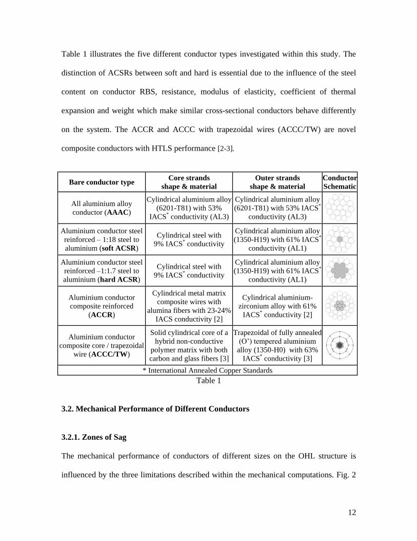
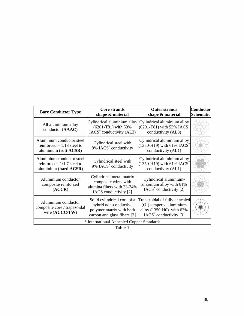
Table 1 illustrates the five different conductor types investigated within this study. The
distinction of ACSRs between soft and hard is essential due to the influence of the steel
content on conductor RBS, resistance, modulus of elasticity, coefficient of thermal
expansion and weight which make similar cross-sectional conductors behave differently
on the system. The ACCR and ACCC with trapezoidal wires (ACCC/TW) are novel
composite conductors with HTLS performance [2-3].
Bare conductor type Core strands
shape & material
Outer strands
shape & material
Conductor
Schematic
All aluminium alloy
conductor (AAAC)
Cylindrical aluminium alloy
(6201-T81) with 53%
IACS* conductivity (AL3)
Cylindrical aluminium alloy
(6201-T81) with 53% IACS*
conductivity (AL3)
Aluminium conductor steel
reinforced – 1:18 steel to
aluminium (soft ACSR)
Cylindrical steel with
9% IACS* conductivity
Cylindrical aluminium alloy
(1350-H19) with 61% IACS*
conductivity (AL1)
Aluminium conductor steel
reinforced –1:1.7 steel to
aluminium (hard ACSR)
Cylindrical steel with
9% IACS* conductivity
Cylindrical aluminium alloy
(1350-H19) with 61% IACS*
conductivity (AL1)
Aluminium conductor
composite reinforced
(ACCR)
Cylindrical metal matrix
composite wires with
alumina fibers with 23-24%
IACS conductivity [2]
Cylindrical aluminium-
zirconium alloy with 61%
IACS* conductivity [2]
Aluminium conductor
composite core / trapezoidal
wire (ACCC/TW)
Solid cylindrical core of a
hybrid non-conductive
polymer matrix with both
carbon and glass fibers [3]
Trapezoidal of fully annealed
(O’) tempered aluminium
alloy (1350-H0) with 63%
IACS* conductivity [3]
* International Annealed Copper Standards
Table 1
3.2. Mechanical Performance of Different Conductors
3.2.1. Zones of Sag
The mechanical performance of conductors of different sizes on the OHL structure is
influenced by the three limitations described within the mechanical computations. Fig. 2
13
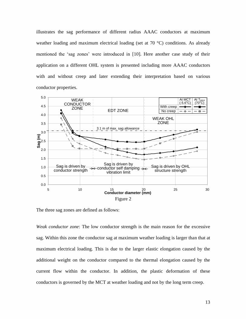
illustrates the sag performance of different radius AAAC conductors at maximum
weather loading and maximum electrical loading (set at 70 °C) conditions. As already
mentioned the ‘sag zones’ were introduced in [10]. Here another case study of their
application on a different OHL system is presented including more AAAC conductors
with and without creep and later extending their interpretation based on various
conductor properties. 14pt
0.0
0.5
1.0
1.5
2.0
2.5
3.0
3.5
4.0
4.5
5.0
5 10 15 20 25 30Conductor diameter (mm)
Sa
g (
m)
Sag at -5.6˚C + ε
Sag at 70˚C + ε
Sag at -5.6˚C
Sag at 70˚C
WEAK CONDUCTOR
ZONEEDT ZONE
Sag is driven by conductor self damping
vibration limit
WEAK OHL ZONE
Sag is driven by OHL structure strength
Sag is driven by conductor strength
At TMAX (70
oC)
At MCT (-5.6
oC)
With creep
No creep
3.1 m of max. sag allowance
Figure 2
The three sag zones are defined as follows:
Weak conductor zone: The low conductor strength is the main reason for the excessive
sag. Within this zone the conductor sag at maximum weather loading is larger than that at
maximum electrical loading. This is due to the larger elastic elongation caused by the
additional weight on the conductor compared to the thermal elongation caused by the
current flow within the conductor. In addition, the plastic deformation of these
conductors is governed by the MCT at weather loading and not by the long term creep.
14
EDT zone: Sag is driven by the conductor self damping vibration limit. This is usually set
as a percentage of RBS and therefore the homogeneous conductors (like the AAACs
illustrated in Fig. 2) - or conductors with constant core to outer strands ratio - within this
zone are expected to have similar sag values. The mechanical performance of conductors
of these sizes can be further improved using vibration dampers and thus increasing the
EDT of the vibration limit which is usually 20% RBS. The creep effect of these
conductors is governed by the long term creep.
Weak OHL zone: Further increase in conductor size results only in an increase of
conductor weight (and not in tension) as MCT is limited by the strength of the OHL
structure, which in turn reduces the system’s EDT. This results in increased sag values
with increased conductor size, as increase of the conductor’s weight stresses the
conductor further causing more elastic elongation. The creep strain for these conductors
is also governed by long term creep; however, since the EDT is reduced compared to the
previous zone, the creep is lower.
It should be noted that the results without creep are obtained when the creep strain is
negated by including an initial over-tension during the conductor installation while the
results with creep consider 10 years of conductor plastic elongation and assume a total
duration of 500 hours for maximum weather loading. This duration is essential to
compute the creep caused by the conductor’s maximum mechanical loading, particularly
for the small conductor sizes within the weak conductor zone, as these conductors are

15
affected more by the maximum weather loading and its duration [30]. The elevated
temperature creep effect is not considered at 70 °C [34].
Fig. 3 illustrates the sag zones of the different conductors erected on the OHL structure
described previously and demonstrates how these are influenced by the system, the
conductor type, and the OHL structure. Novel composite conductors of smaller sizes
have not (yet) been produced by the manufactures and therefore only one boundary is
illustrated for these conductors. It is important to emphasise that the RBS of ACCC/TW
is computed by considering only the composite core and totally neglecting the aluminium
strands [3] while in all other conductor types the RBS is the result of the whole conductor
(i.e. combining the strength of core and outer strands).
The EDT zone is reduced as the strength of conductor material(s) is increased; the arrows
illustrate the shift of the boundaries of this zone for the different conductor types. In
particular, by observing the boundaries one can tell which conductor is the strongest.
Consequently, it can be seen that the AAACs are weaker than the hard ACSRs since the
latter have smaller EDT zone. In contrast to the hard ACSRs, the soft ones are weaker
than the AAAC conductors forming wider EDT zone. The slope of increase in sag within
the weak OHL zone is the same for all the conductors since the OHL strength governs
their mechanical performance (sag). Another important observation that can be derived
from the sag zones is that the conductor with the best electro-mechanical performance is
the one with size closed to the boundary of EDT and weak OHL zones. However, if the
ground clearance permitted by the structure allows the installation of a larger conductor
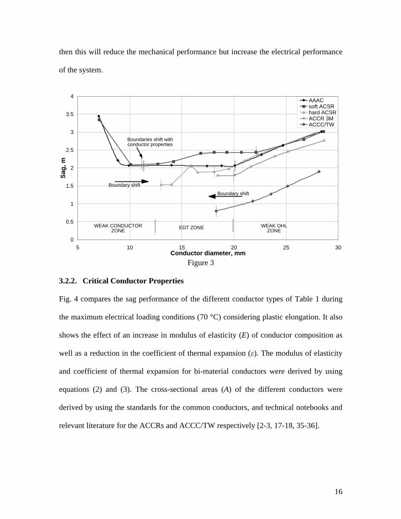
16
then this will reduce the mechanical performance but increase the electrical performance
of the system.
52pt
0
0.5
1
1.5
2
2.5
3
3.5
4
5 10 15 20 25 30Conductor diameter, mm
Sag
, m
AAACsoft ACSRhard ACSRACCR 3MACCC/TW
52pt
0.5
1
1.5
2
2.5
3
3.5
4
4.5
5 10 15 20 25 30Conductor diameter, mm
Sa
g,
m
AAACsoft ACSRhard ACSRACCR 3MACCC/TW
WEAK CONDUCTOR ZONE
EDT ZONE WEAK OHL ZONE
Boundary shift
Boundaries shift with conductor properties
52pt
0.5
1
1.5
2
2.5
3
3.5
4
4.5
5 10 15 20 25 30Conductor diameter, mm
Sa
g,
m
AAACsoft ACSRhard ACSRACCR 3MACCC/TW
52pt
0.5
1
1.5
2
2.5
3
3.5
4
4.5
5 10 15 20 25 30Conductor diameter, mm
Sa
g,
mAAACsoft ACSRhard ACSRACCR 3MACCC/TW
Boundary shift
52pt
0.5
1
1.5
2
2.5
3
3.5
4
4.5
5 10 15 20 25 30Conductor diameter, mm
Sa
g,
m
AAACsoft ACSRhard ACSRACCR 3MACCC/TW
Figure 3
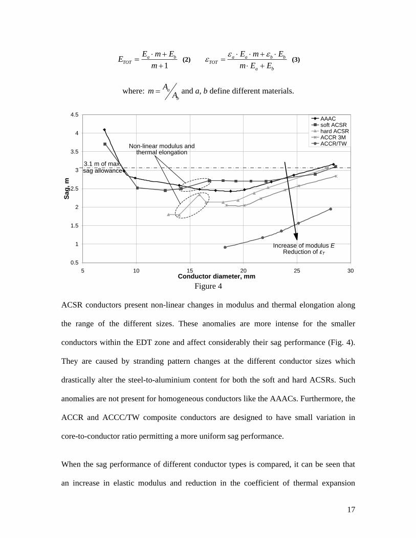
3.2.2. Critical Conductor Properties
Fig. 4 compares the sag performance of the different conductor types of Table 1 during
the maximum electrical loading conditions (70 °C) considering plastic elongation. It also
shows the effect of an increase in modulus of elasticity (E) of conductor composition as
well as a reduction in the coefficient of thermal expansion (ε). The modulus of elasticity
and coefficient of thermal expansion for bi-material conductors were derived by using
equations (2) and (3). The cross-sectional areas (A) of the different conductors were
derived by using the standards for the common conductors, and technical notebooks and
relevant literature for the ACCRs and ACCC/TW respectively [2-3, 17-18, 35-36].
17
1
a bTOT
E m EE
m
(2)
a a b bTOT
a b
E m E
m E E
(3)
where: a
b
Am
A and a, b define different materials.
52pt
0.5
1
1.5
2
2.5
3
3.5
4
4.5
5 10 15 20 25 30Conductor diameter, mm
Sag
, m
AAACsoft ACSRhard ACSRACCR 3MACCR/TW
Increase of modulus EReduction of εT
Non-linear modulus and thermal elongation
52pt
0.5
1
1.5
2
2.5
3
3.5
4
4.5
5 10 15 20 25 30Conductor diameter, mm
Sag
, m
AAACsoft ACSRhard ACSRACCR 3MACCC/TW
52pt
0.5
1
1.5
2
2.5
3
3.5
4
4.5
5 10 15 20 25 30Conductor diameter, mm
Sag
, m
AAACsoft ACSRhard ACSRACCR 3MACCC/TW
3.1 m of max. sag allowance
52pt
0.5
1
1.5
2
2.5
3
3.5
4
4.5
5 10 15 20 25 30Conductor diameter, mm
Sag
, m
AAACsoft ACSRhard ACSRACCR 3MACCC/TW
Figure 4
ACSR conductors present non-linear changes in modulus and thermal elongation along
the range of the different sizes. These anomalies are more intense for the smaller
conductors within the EDT zone and affect considerably their sag performance (Fig. 4).
They are caused by stranding pattern changes at the different conductor sizes which
drastically alter the steel-to-aluminium content for both the soft and hard ACSRs. Such
anomalies are not present for homogeneous conductors like the AAACs. Furthermore, the
ACCR and ACCC/TW composite conductors are designed to have small variation in
core-to-conductor ratio permitting a more uniform sag performance.
When the sag performance of different conductor types is compared, it can be seen that
an increase in elastic modulus and reduction in the coefficient of thermal expansion
18
results in sag mitigation. ACCC/TWs develop the smallest sag values, which illustrates
the very low thermal elongation factor of their composite core when compared to other
conductor types [3]. ACCRs have the second best performance.
ACCC/TWs are lighter compared to hard ACSRs of equivalent diameter but heavier than
the AAACs and soft ACSRs as the trapezoidal shape wires increase the amount of
aluminium for the same conductor outer diameter [10]. Hence, the approximately 16%
heavier ACCC/TW sags much less than the AAAC and soft ACSR of similar diameter.
Their sag performance at maximum electrical loading conditions (70 °C) is also better
than the performance of ACCRs. However, the large difference of thermal expansion
coefficient between the composite core and aluminium strands for the ACCC/TW
increases the risk of developing bird cages (i.e. the separation of the outer conductor
strands from the core) in long spans with loss of structural integrity, at very high
operating temperatures [3, 37].
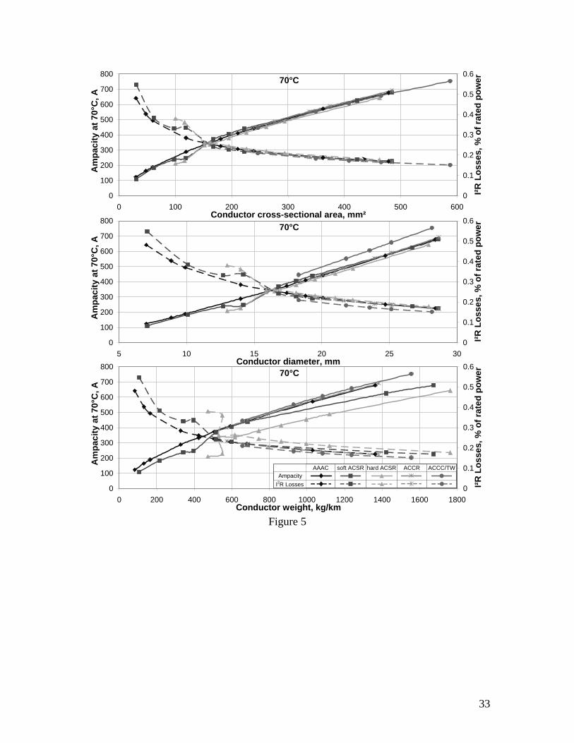
3.3. Electrical Performance: Ampacity & Losses
By increasing the conductor diameter the current capacity is increased, raising the
maximum power rating of the OHL. The maximum conductor diameter size, though, is
limited by the permitted sag on the particular system. For this reason, in the example of
the system studied here, the conductors above the dotted lines of Fig. 4 could not be used
for re-conductoring. Fig. 5 illustrates the exact ampacities for the different conductors at
70 °C, by their total cross-sectional area (A), diameter and weight. The changes in steel-
to-aluminium ratio over the range of sizes of the soft and hard ACSRs also affect their
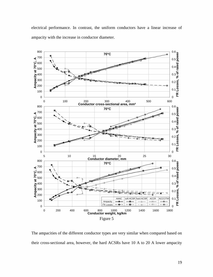
19
electrical performance. In contrast, the uniform conductors have a linear increase of
ampacity with the increase in conductor diameter.
pp 14pt
0
100
200
300
400
500
600
700
800
0 200 400 600 800 1000 1200 1400 1600 1800Conductor weight, kg/km
Am
pa
cit
y a
t 7
0°C
, A
0
0.1
0.2
0.3
0.4
0.5
0.6
I²R
Lo
ss
es
, %
of
rate
d p
ow
er
70°C
pp 14pt
0
100
200
300
400
500
600
700
800
0 100 200 300 400 500 600Conductor cross-sectional area, mm²
Am
pa
cit
y a
t 7
0°C
, A
0
0.1
0.2
0.3
0.4
0.5
0.6
I²R
Lo
ss
es
, %
of
rate
d p
ow
er
70°C
pp 14pt
0
100
200
300
400
500
600
700
800
5 10 15 20 25 30Conductor diameter, mm
Am
pa
cit
y a
t 7
0°C
, A
0
0.1
0.2
0.3
0.4
0.5
0.6
I²R
Lo
ss
es
, %
of
rate
d p
ow
er
70°C
Ampacity
I2R Losses
AAAC soft ACSR hard ACSR ACCR ACCC/TW
Figure 5
The ampacities of the different conductor types are very similar when compared based on
their cross-sectional area, however, the hard ACSRs have 10 A to 20 A lower ampacity

20
than the equivalent conductors of other types and develop more I2R losses. This is the
result of their larger volume resistivity compared to the soft ACSRs and AAACs, and
their steel core losses which are introduced by the increased steel content when compared
to soft ACSRs [38]. Another important observation regards the lower losses of the
ACCC/TW conductors when compared with the equivalent in diameter aluminium based
conductors (i.e. AAACs and ACCRs) considering that their composite core is a non-
conductive compound. This is due to the trapezoidal aluminium strands.
Finally, when the electrical performance of the conductors is compared based on their
weight the poor performance of the ACSR conductors is obvious and more noticeable for
the hard ones. On the other hand, the ACCC/TWs appear to have the best performance.
The comparison of the conductors in respect to their electrical performance based on their
weight is considered to be the most informative one, since weight also defines the
maximum conductor size that can be installed on the system.
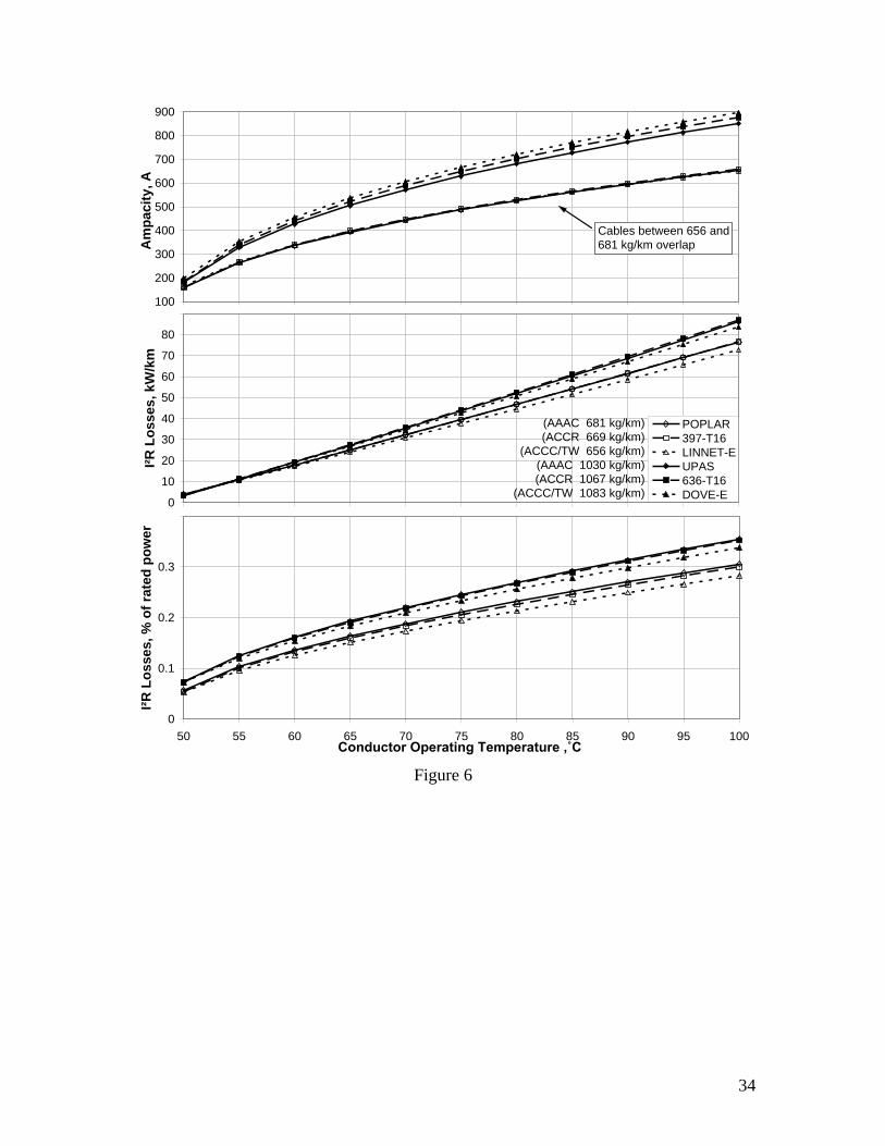
3.3. Holistic (Electro-Mechanical) Comparison of Equivalent Weight Conductors
Given the previous results, Fig. 6 shows further comparisons of conventional AAAC
conductors and equivalent weight novel conductors at different TMAX in respect to their
electrical performance on this system.

21
ACCC/TW, ACCR, and AAAC comparison of the same weight condcutor sizes (33kV line)
0
10
20
30
40
50
60
70
80
90
50 55 60 65 70 75 80 85 90 95 100Conductor Operating Temperature, ˚C
I²R
Lo
sses
, k
W/k
m
POPLAR
397-T16
LINNET-E
UPAS
636-T16
DOVE-E
ACCC/TW, ACCR, and AAAC comparison of the same weight condcutor sizes (33kV line)
100
200
300
400
500
600
700
800
900
50 55 60 65 70 75 80 85 90 95 100Conductor Operating Temperature, ˚C
Am
pacit
y, A
POPLAR
397-T16
LINNET-E
UPAS
636-T16
DOVE-E
ACCC/TW, ACCR, and AAAC comparison of the same weight condcutor sizes (33kV line)
0
0.1
0.2
0.3
0.4
50 55 60 65 70 75 80 85 90 95 100Conductor Operating Temperature ,˚C
I²R
Lo
sses, %
of
rate
d p
ow
er
POPLAR
397-T16
LINNET-E
UPAS
636-T16
DOVE-E
(AAAC 681 kg/km)
(ACCR 669 kg/km)
(ACCC/TW 656 kg/km)
(AAAC 1030 kg/km)
(ACCR 1067 kg/km)
(ACCC/TW 1083 kg/km)
Cables between 656 and
681 kg/km overlap
Figure 6
The comparison of the heavier conductors (362-L3 (Upas), 636-T16, and Dove-E)
indicates that the ACCC/TW allows more ampacity than the equivalent weight ACCR
and AAAC and produces lower losses (Fig. 6). In contrast, comparison of lighter
conductors (Linnet-E, 239-AL3 (Poplar) and 397-T16) shows that they have almost
identical ampacities. However, the ACCC/TW conductor appears to have lower losses,

22
particularly at higher temperatures (i.e. 1.6 and 3 kW/km at 70 °C and 90 °C,
respectively, when compared to the Poplar) indicating their lower resistance. Their
normalised losses to the maximum power rating appear to have 5% difference at 70 °C
which further increases to 10% at 90 °C in favour of the ACCC/TW’s performance.
It should be noted that even though ACCC/TWs may operate at higher temperatures
allowing greater ampacities, the analysis for this paper focuses on their operation at lower
temperatures to keep their losses to values similar to conventional conductors.
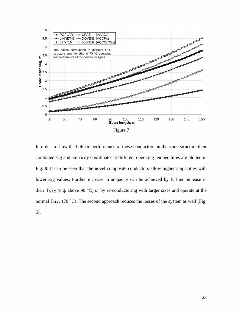
The mechanical performance of the same conductors is compared in Fig. 7 for different
OHL span lengths at 70 °C. Fig. 7, in combination with previous results (Figs 3 and 4),
indicates that when the equivalent weight conductors are compared, the increase in sag
caused by the increase in span length is steeper for those with smaller modulus and larger
thermal elongation (see difference in the slopes of the lines for Linet-E compared to
Poplar and 397-T16). Furthermore, the comparison of conductors of the same technology
based on their weight (Fig. 7) highlights the weight effect on sag, given by the steeper
increase in sag for the heavier conductors. This demonstrates the importance of the
implementation of lightweight conductor technologies particularly at weak wood pole
OHL structures.
23
IET Paper
0
0.5
1
1.5
2
2.5
3
3.5
4
4.5
5
50 60 70 80 90 100 110 120 130 140 150Span length, m
Co
nd
uc
tor
sa
g,
m
POPLAR UPASLINNET-E DOVE-E397-T16 636-T16
(AAACs)(ACCRs) (ACCC/TWs)
The points correspond to different OHL
structure span lengths at 70 °C operating
temperature for all the conductor types.
Figure 7
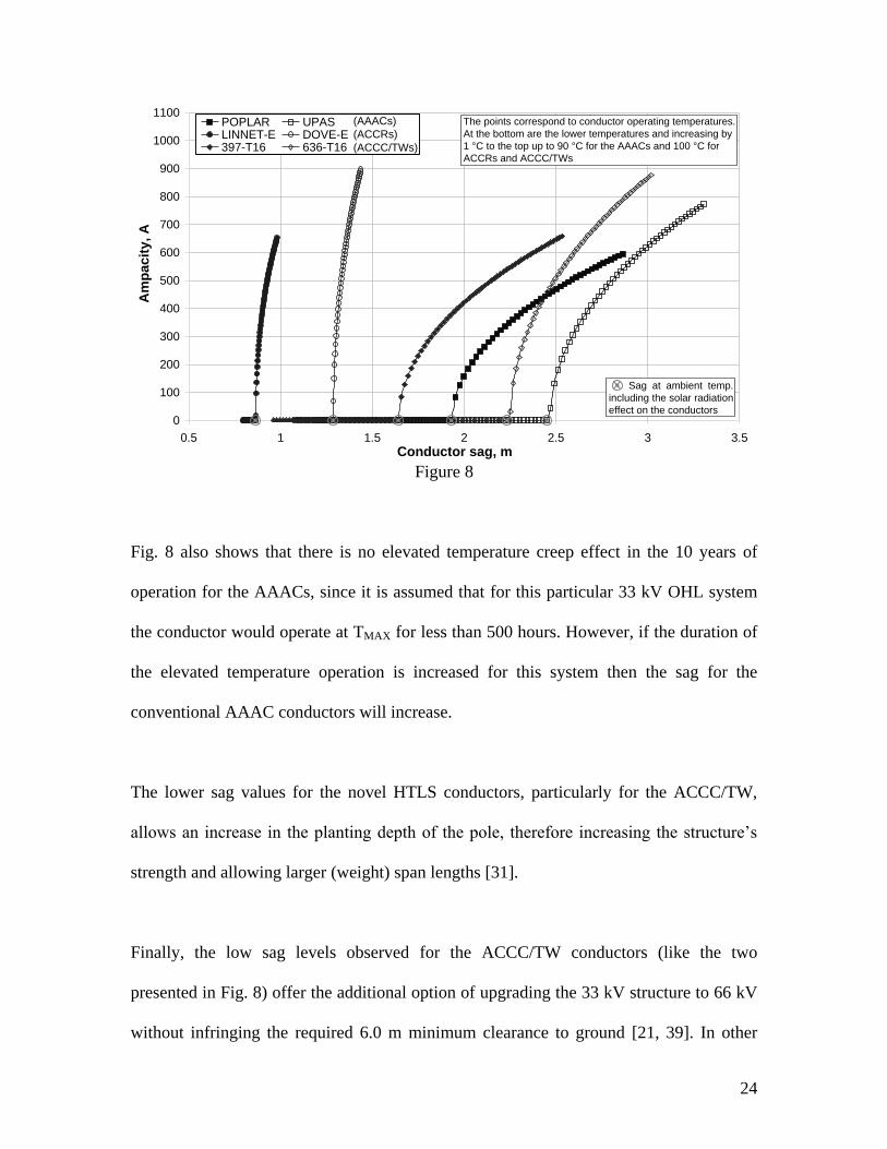
In order to show the holistic performance of these conductors on the same structure their
combined sag and ampacity coordinates at different operating temperatures are plotted in
Fig. 8. It can be seen that the novel composite conductors allow higher ampacities with
lower sag values. Further increase in ampacity can be achieved by further increase in
their TMAX (e.g. above 90 °C) or by re-conductoring with larger sizes and operate at the
normal TMAX (70 °C). The second approach reduces the losses of the system as well (Fig.
6).
24
IET Paper
0
100
200
300
400
500
600
700
800
900
1000
1100
0.5 1 1.5 2 2.5 3 3.5
Conductor sag, m
Am
pacit
y, A
POPLAR UPASLINNET-E DOVE-E397-T16 636-T16
The points correspond to conductor operating temperatures.
At the bottom are the lower temperatures and increasing by
1 °C to the top up to 90 °C for the AAACs and 100 °C for
ACCRs and ACCC/TWs
(AAACs)
(ACCRs)
(ACCC/TWs)
Sag at ambient temp.
including the solar radiation
effect on the conductors
Figure 8
Fig. 8 also shows that there is no elevated temperature creep effect in the 10 years of
operation for the AAACs, since it is assumed that for this particular 33 kV OHL system
the conductor would operate at TMAX for less than 500 hours. However, if the duration of
the elevated temperature operation is increased for this system then the sag for the
conventional AAAC conductors will increase.
The lower sag values for the novel HTLS conductors, particularly for the ACCC/TW,
allows an increase in the planting depth of the pole, therefore increasing the structure’s
strength and allowing larger (weight) span lengths [31].
Finally, the low sag levels observed for the ACCC/TW conductors (like the two
presented in Fig. 8) offer the additional option of upgrading the 33 kV structure to 66 kV
without infringing the required 6.0 m minimum clearance to ground [21, 39]. In other
25
words, when the 33 kV structure with a conventional conductor is re-conductored with an
equivalent in weight ACCC/TW the ground clearance is increased by approximately 1 m
when the creep is negated (Fig. 3). This increases further to 1.5 m when the AAAC is not
initially over-tensioned for the required creep negation (Fig. 8). It is important to
emphasize that this conductor develops larger sag values during the maximum weather
loading.
4. Conclusions
The comparative study of the different conductors on this 33 kV OHL structure, firstly
shows that from the conventional conductors the AAACs have better electrical and
mechanical performance, particularly when initial over-stressing is applied to negate the
creep-strain effect. AAACs have better ampacity-to-weight ratio, thus they stress the
OHL structure less, which potentially allows re-conductoring with larger conductors
without the need of structure and foundation reinforcement. Soft ACSRs are in general
heavier than the AAACs and consequently impractical for the comparatively weak wood
pole structures, although their electrical performance is not very different. Hard ACSRs
are very heavy and thus unsuitable for most wood pole applications.
Another substantial finding involves the new composite HTLS conductors which can
increase the power transfer of the 33 kV wood pole system either through increased
operating temperatures or re-conductoring with larger conductors. ACCC/TW conductors
have very low sag values, as a result of the very low thermal expansion coefficient and
density as well as a high modulus of elasticity. This allows the following options, or
combination of them, for improving system performance:
26
Increasing the span length of the structure and hence reducing the number of
poles needed.
Reducing the height of the structure requirements or increasing the planting depth
and therefore the structure’s strength particularly in “weak” ground.
Increasing the maximum operating temperature of the conductor.
Re-conductoring with larger conductors.
Increasing the voltage level of the OHL structure to 66 kV.
The last three points increase the power capacity of the structure with minimum structural
changes, while the last two reduce the losses as well.
As a concluding remark, an ‘ideal’ conductor for operation at normal operating
temperatures on weak structure systems can be identified based on conductors’ properties
and their effect on system’s performance, as reported in this paper. Such a conductor
would have low density strength member, high strength and low coefficient of thermal
expansion combined with high compaction and low resistance-to-weight soft outer
strands. This design could offer potential benefits for the performance of relatively weak
wood pole structures, such as the one investigated here.
Acknowledgment
This work is funded through the EPSRC Supergen V, UK Energy Infrastructure
(AMPerES) grant in collaboration with UK electricity network operators working under
Ofgem's Innovation Funding Incentive scheme; - full details on http://www.supergen-
amperes.org

27
References
[1] IEC 61597: Overhead Electrical Conductors - Calculation Methods for Stranded
Bare Conductors. International Electrotechnical Commission. May 1995.
[2] 3M. Aluminum Conductor Composite Reinforced Technical Notebook (477 kcmil
family) Conductor & Accessory Testing, 2006: Available from:
http://www.energy.ca.gov/2004_policy_update/documents/2004-06-14-
workshop/public_comments/2004-06-28_3M_PART2.PDF.
[3] Alawar A, Bosze EJ, Nutt SR. A composite core conductor for low sag at high
temperatures. IEEE Transactions on Power Delivery. 2005;20(3): 2193-9.
[4] Zamora I, Mazon AJ, Eguia P, Criado R, Alonso C, Iglesias J, et al., editors.
High-temperature conductors: a solution in the uprating of overhead transmission lines.
IEEE Power Tech Proceedings, Porto-Portugal; 2001.
[5] Shankle DF. Incremental Voltage Uprating of Transmission Lines. IEEE
Transactions on Power Apparatus and Systems. 1971;PAS-90(4): 1791-5.
[6] Albizu I, Mazon AJ, Zamora I, editors. Methods for increasing the rating of
overhead lines. Power Tech, 2005 IEEE Russia; 2005.
[7] Kotaka S, Itou H, Matsuura T, Yonezawa K, Morikawa H. Applications of Gap-
type Small-Sag Conductors for Overhead Transmission Lines. SEI Technical Review.
[SEI Technical Review]. Jun. 2000(SEI Technical Review, No 50): 64-72.
[8] Adams HW. Steel Supported Aluminum Conductors (SSAC) for Overhead
Transmission Lines. IEEE Transactions on Power Apparatus and Systems. 1974;PAS-
93(5): 1700-5.
[9] Exposito AG, Santos JR, Cruz Romero P. Planning and Operational Issues
Arising From the Widespread Use of HTLS Conductors. IEEE Transactions on Power
Systems. 2007;22(4): 1446-55.
[10] Kopsidas K, Rowland SM. A Performance Analysis of Reconductoring an
Overhead Line Structure. IEEE Transactions on Power Delivery. 2009;24(4): 2248-56.
[11] Kopsidas K. Modelling Thermal Rating of Arbitrary Overhead Line Systems
[PhD Thesis]. Manchester, UK: The University of Manchester; 2009.
[12] Kopsidas K, Rowland SM. A Holistic Method for a Conductor’s Ampacity and
Sag Computation on an OHL Structure. IEEE Transactions on Power Delivery. under
review.
[13] BS EN 50182: Conductors for Overhead Lines - Round Wire Concentric Lay
Stranded Conductors. British Standards. 2001.
[14] CIGRE SC.B2 - WG.B2.12: Sag-Tension Calculation Methods for Overhead
Lines. 2007.
[15] ASTM B 193-02: Test Method for Resistivity of Electrical Conductor Materials.
Annual Book of ASTM Standards. 2005;02.03: 68-72.
[16] ASTM B 230/B 230M-99: Specification for Aluminum 1350-H19 Wire for
Electrical Purposes. Annual Book of ASTM Standards. 2005;02.03: 91-4.
[17] ASTM B 498/B 498M-98(2002): Specification for Zinx-Coated (Galvanized)
Steel Core Wire for Aluminum Conductors, Steel Reinforced (ACSR). Annual Book of
ASTM Standards. 2005;02.03: 218-21.
28
[18] ASTM B 779 - 03: Standard Specification for Shaped Wire Compact Concentric-
Law-Stranded Aluminum Conductors, Steel Reinforced (ACSR/TW). Annual Book of
ASTM Standards. 2005;02.03: 309-14.
[19] ASTM B232/B 232M-01: Specification for Concentric-Lay-Stranded Aluminum
Conductors, Coated-Steel Reinforced (ACSR). Annual Book of ASTM Standards. 2005:
106-21.
[20] ENATS 43-40: Single Circuit Overhead Lines on Wood Poles for Use at High
Voltage Up to and Including 33kV. Energy Networks Association Technical
Specifications. Issue 2, 2004(2).
[21] BS EN 50341-3: Overhead electrical lines exceeding AC 45 kV - Part 3: Set of
National Normative Aspects. British Standards. 2001.
[22] Dwight HB. Skin Effect in Tubular and Flat Conductors. AIEE Transactions.
1918;37: 1379-403.
[23] Lewis WA, Tuttle PD. The Resistance and Reactance of Aluminum Conductors,
Steel Reinforced. AIEE Transactions. 1959;77(3): 1189-215.
[24] Olver FWJ. 9. Bessel Functions of Integer Order. In: Abramowitz M, Stegun IA,
editors. Handbook of Mathematical Functions. Washington, D. C.: U. S. Dept.
Commerce; 1964. p. 378-85.
[25] Howington BS, Rathbun LS. AC Resistance of ACSR - Magnetic and
Temperature Effects. IEEE Transactions on Power Apparatus and Systems. 1985;PAS-
104(6): 1578-84.
[26] Kirkpatrick L, (Ed.). Aluminum Electrical Conductor Handbook. Third ed.
Washington, D.C.: the Aluminum Association; 1989.
[27] IEEE Standard for Calculating the Current-Temperature of Bare Overhead
Conductors. IEEE Std 738-2006 (Revision of IEEE Std 738-1993). 2007: 1-59.
[28] Harvey JR, Larson RE. Creep Equations of Conductors for Sag-Tension
Calculations. IEEE/PES Winter Meeting Conference. Paper No. C71 190-2, 1972.
[29] Harvey JR, Larson RE. Use of Elevated-Temperature Creep Data in Sag-Tension
Calculations. IEEE Transactions on Power Apparatus and Systems. 1970;PAS-89, No 3:
380-6.
[30] CIGRE SC22 - WG05: Permanent elongation of conductors. Predictor equation
and evaluation methods. Electra N° 75. 1981: 63-98.
[31] BS 1990-1: Wood poles for overhead power and telecommunication lines - Part
1: Specification for soft wood poles. British Standards. 1984.
[32] BS EN 50423-3: Overhead electrical lines exceeding AC 1 kV up to and
including AC 45 kV - Part 3: Set of National Normative Aspects. British Standards.
2005.
[33] BS EN 50423-1: Overhead electrical lines exceeding AC 1 kV up to and
including AC 45 kV - Part 1: General requirements - Common specifications. British
Standards. 2005.
[34] IEEE Guide for Determining the Effects of High-Temperature Operation on
Conductors, Connectors, and Accessories. IEEE Std 1283-2004. 2005: 1-28.
[35] Development of Stress-strain Polynomials and Creep Parameters for ACCC/TW
Conductors, 2008 Jul. 12: Available from:
www.powline.com/files/cables/ctc_conductors.pdf.

29
[36] ASTM B 398/B 398M-02: Standard Specification for Aluminum-Alloy 6201-T81
Wire for Electrical Purposes. Annual Book of ASTM Standards. 2005;02.03: 178-81.
[37] Nigol O, Barrett JS. Characteristics of ACSR Conductors at High Temperatures
and Stresses. IEEE Transactions on Power Apparatus and Systems. 1981;PAS-100(2):
485-93.
[38] Morgan VT, editor. Electrical Characteristics of Steel-Cored Aluminium
Conductors. IEEE Proceedings; Feb. 1965; London.
[39] BS EN 50341-1: Overhead electrical lines exceeding AC 45 kV - Part 1: General
requirements - Common specifications. British Standards. 2001.
List of Table & Figures Captions
Table 1: Properties of the different types of conductors studied.
Figure 1: Summary flowchart for the methodology for sag and ampacity calculations.
Figure 2: AAAC sag performance at maximum designed weather loading and operating
temperature.
Figure 3: Sag zones of different conductor types at 70 °C without creep.
Figure 4: Sag performance of different conductor types at 70 °C including creep.
Figure 5: Electrical performance of different conductor types.
Figure 6: Electrical performance of conductors of similar-weight at different maximum
operating temperatures.
Figure 7: Sag performance of different type but similar-weight conductors for different
spans.
Figure 8: Plots of sag and ampacity of similar-weight conductors at different operating
temperatures.
30
Bare Conductor Type Core strands
shape & material
Outer strands
shape & material
Conductor
Schematic
All aluminium alloy
conductor (AAAC)
Cylindrical aluminium alloy
(6201-T81) with 53%
IACS* conductivity (AL3)
Cylindrical aluminium alloy
(6201-T81) with 53% IACS*
conductivity (AL3)
Aluminium conductor steel
reinforced – 1:18 steel to
aluminium (soft ACSR)
Cylindrical steel with
9% IACS* conductivity
Cylindrical aluminium alloy
(1350-H19) with 61% IACS*
conductivity (AL1)
Aluminium conductor steel
reinforced –1:1.7 steel to
aluminium (hard ACSR)
Cylindrical steel with
9% IACS* conductivity
Cylindrical aluminium alloy
(1350-H19) with 61% IACS*
conductivity (AL1)
Aluminium conductor
composite reinforced
(ACCR)
Cylindrical metal matrix
composite wires with
alumina fibers with 23-24%
IACS conductivity [2]
Cylindrical aluminium-
zirconium alloy with 61%
IACS* conductivity [2]
Aluminium conductor
composite core / trapezoidal
wire (ACCC/TW)
Solid cylindrical core of a
hybrid non-conductive
polymer matrix with both
carbon and glass fibers [3]
Trapezoidal of fully annealed
(O’) tempered aluminium
alloy (1350-H0) with 63%
IACS* conductivity [3]
* International Annealed Copper Standards
Table 1

31
Electrical computation
Ageing computation
Overhead Line
DataOperational Data
Newton-Raphson
iteration of Change
of State Equation
Conductor Tension & Sag
Conductor Ampacity
Conductor RAC
at TOPERATING & ƒSYSTEM
Weather Data Conductor Data
Conductor Creep (IEEE Std)
(Creep-Strain Curves)
Final System
Conditions
Ampacity calculation(IEEE 738 Std)
Conductor Tension & Sag with creep
Maximum conductor tension (MCT)
Conductor Tension & Sag when creep is negated
Mechanical computation
At specified loading conditions
VIBRATION
LIMIT
STRUCTURE
LIMIT
CONDUCTOR
LIMIT
At TOPERATING (oC)
Figure 1
14pt
0.0
0.5
1.0
1.5
2.0
2.5
3.0
3.5
4.0
4.5
5.0
5 10 15 20 25 30Conductor diameter (mm)
Sa
g (
m)
Sag at -5.6˚C + ε
Sag at 70˚C + ε
Sag at -5.6˚C
Sag at 70˚C
WEAK CONDUCTOR
ZONEEDT ZONE
Sag is driven by conductor self damping
vibration limit
WEAK OHL ZONE
Sag is driven by OHL structure strength
Sag is driven by conductor strength
At TMAX (70
oC)
At MCT (-5.6
oC)
With creep
No creep
2.8m of max. sag allowance
Figure 2

32
52pt
0
0.5
1
1.5
2
2.5
3
3.5
4
5 10 15 20 25 30Conductor diameter, mm
Sag
, m
AAACsoft ACSRhard ACSRACCR 3MACCC/TW
52pt
0.5
1
1.5
2
2.5
3
3.5
4
4.5
5 10 15 20 25 30Conductor diameter, mm
Sa
g,
m
AAACsoft ACSRhard ACSRACCR 3MACCC/TW
WEAK CONDUCTOR ZONE
EDT ZONE WEAK OHL ZONE
Boundary shift
Boundaries shift with conductor properties
52pt
0.5
1
1.5
2
2.5
3
3.5
4
4.5
5 10 15 20 25 30Conductor diameter, mm
Sa
g,
m
AAACsoft ACSRhard ACSRACCR 3MACCC/TW
52pt
0.5
1
1.5
2
2.5
3
3.5
4
4.5
5 10 15 20 25 30Conductor diameter, mm
Sa
g,
m
AAACsoft ACSRhard ACSRACCR 3MACCC/TW
Boundary shift
52pt
0.5
1
1.5
2
2.5
3
3.5
4
4.5
5 10 15 20 25 30Conductor diameter, mm
Sa
g,
m
AAACsoft ACSRhard ACSRACCR 3MACCC/TW
Figure 3
52pt
0.5
1
1.5
2
2.5
3
3.5
4
4.5
5 10 15 20 25 30Conductor diameter, mm
Sag
, m
AAACsoft ACSRhard ACSRACCR 3MACCR/TW
Increase of modulus EReduction of εT
Non-linear modulus and thermal elongation
52pt
0.5
1
1.5
2
2.5
3
3.5
4
4.5
5 10 15 20 25 30Conductor diameter, mm
Sag
, m
AAACsoft ACSRhard ACSRACCR 3MACCC/TW
52pt
0.5
1
1.5
2
2.5
3
3.5
4
4.5
5 10 15 20 25 30Conductor diameter, mm
Sag
, m
AAACsoft ACSRhard ACSRACCR 3MACCC/TW
3.1 m of max. sag allowance
52pt
0.5
1
1.5
2
2.5
3
3.5
4
4.5
5 10 15 20 25 30Conductor diameter, mm
Sag
, m
AAACsoft ACSRhard ACSRACCR 3MACCC/TW
Figure 4
33
pp 14pt
0
100
200
300
400
500
600
700
800
0 200 400 600 800 1000 1200 1400 1600 1800Conductor weight, kg/km
Am
pa
cit
y a
t 7
0°C
, A
0
0.1
0.2
0.3
0.4
0.5
0.6
I²R
Lo
ss
es
, %
of
rate
d p
ow
er
70°C
pp 14pt
0
100
200
300
400
500
600
700
800
0 100 200 300 400 500 600Conductor cross-sectional area, mm²
Am
pa
cit
y a
t 7
0°C
, A
0
0.1
0.2
0.3
0.4
0.5
0.6
I²R
Lo
ss
es
, %
of
rate
d p
ow
er
70°C
pp 14pt
0
100
200
300
400
500
600
700
800
5 10 15 20 25 30Conductor diameter, mm
Am
pa
cit
y a
t 7
0°C
, A
0
0.1
0.2
0.3
0.4
0.5
0.6
I²R
Lo
ss
es
, %
of
rate
d p
ow
er
70°C
Ampacity
I2R Losses
AAAC soft ACSR hard ACSR ACCR ACCC/TW
Figure 5
34
ACCC/TW, ACCR, and AAAC comparison of the same weight condcutor sizes (33kV line)
0
10
20
30
40
50
60
70
80
90
50 55 60 65 70 75 80 85 90 95 100Conductor Operating Temperature, ˚C
I²R
Lo
sses
, k
W/k
m
POPLAR
397-T16
LINNET-E
UPAS
636-T16
DOVE-E
ACCC/TW, ACCR, and AAAC comparison of the same weight condcutor sizes (33kV line)
100
200
300
400
500
600
700
800
900
50 55 60 65 70 75 80 85 90 95 100Conductor Operating Temperature, ˚C
Am
pacit
y, A
POPLAR
397-T16
LINNET-E
UPAS
636-T16
DOVE-E
ACCC/TW, ACCR, and AAAC comparison of the same weight condcutor sizes (33kV line)
0
0.1
0.2
0.3
0.4
50 55 60 65 70 75 80 85 90 95 100Conductor Operating Temperature ,˚C
I²R
Lo
sses, %
of
rate
d p
ow
er
POPLAR
397-T16
LINNET-E
UPAS
636-T16
DOVE-E
(AAAC 681 kg/km)
(ACCR 669 kg/km)
(ACCC/TW 656 kg/km)
(AAAC 1030 kg/km)
(ACCR 1067 kg/km)
(ACCC/TW 1083 kg/km)
Cables between 656 and
681 kg/km overlap
Figure 6

35
IET Paper
0
0.5
1
1.5
2
2.5
3
3.5
4
4.5
5
50 60 70 80 90 100 110 120 130 140 150Span length, m
Co
nd
uc
tor
sa
g,
m
POPLAR UPASLINNET-E DOVE-E397-T16 636-T16
(AAACs)(ACCRs) (ACCC/TWs)
The points correspond to different OHL
structure span lengths at 70 °C operating
temperature for all the conductor types.
Figure 7 IET Paper
0
100
200
300
400
500
600
700
800
900
1000
1100
0.5 1 1.5 2 2.5 3 3.5
Conductor sag, m
Am
pacit
y, A
POPLAR UPASLINNET-E DOVE-E397-T16 636-T16
The points correspond to conductor operating temperatures.
At the bottom are the lower temperatures and increasing by
1 °C to the top up to 90 °C for the AAACs and 100 °C for
ACCRs and ACCC/TWs
(AAACs)
(ACCRs)
(ACCC/TWs)
Sag at ambient temp.
including the solar radiation
effect on the conductors
Figure 8